An Enhanced Physics-Informed Neural Network with Spatial RBF Embedding and Temporal Initial Condition Embedding for the Allen–Cahn Equation

Abstract

Phase field models are widely employed in materials science, fluid dynamics, fracture mechanics, and image processing to describe physical processes involving complex interface evolution, with the Allen–Cahn equation serving as a classic example. Physics-informed neural networks (PINNs) have been extensively applied to various partial differential equations, but their accuracy in solving the Allen–Cahn equation is often compromised due to the sharp variations of the equation’s solution across phase interfaces. This paper proposes an enhanced PINN with spatial and temporal feature embedding strategies (STFE-PINN) for solving the Allen–Cahn equation. Specifically, for the spatial embedding, the input spatial coordinates are passed through a radial basis function (RBF) neural network, and its output is embedded as a feature into the PINN. By incorporating learnable shape parameters, the RBF embedding adaptively adjusts its basis functions, which strengthens the PINN’s ability to capture high-frequency spatial features and steep gradients. For the temporal embedding, the initial condition is embedded as an additional feature. This strategy enables the network to retain the information of the initial condition throughout training, thereby improving the learning of the phase field evolution and enhancing the accuracy of the PINN. Numerical experiments in one, two, and three dimensions validate the effectiveness and stability of the proposed method.

1. Introduction

Phase field models provide a fundamental framework for describing moving interface problems in materials science [1], fluid mechanics [2], fracture mechanics [3,4], and image processing [5]. As a prototypical example, the Allen–Cahn equation plays a key role in understanding phase transitions and curvature-driven flows. Specifically, the Allen–Cahn equation is given by

$${\displaystyle \frac{\partial u}{\partial t}}=\mu \left(u\right)({\epsilon }^2\mathrm{\Delta }u-f\left(u\right)),(\mathit{x},t)\in \mathrm{\Omega }\times (0,T],$$

(1)

subject to the initial condition

$$u(\mathit{x},0)=u_0\left(\mathit{x}\right),\mathit{x}\in \mathrm{\Omega },$$

(2)

and appropriate boundary conditions, such as Dirichlet, Neumann, or periodic conditions. Here, u denotes the phase field variable, $\mathrm{\Omega }\subset {\mathbb{R}}^d$ is a bounded domain, and $\epsilon >0$ is a small parameter representing the interfacial width. As $\epsilon \to 0$, the solution develops sharp transitions at the phase interface. The mobility function $\mu \left(u\right)$ is typically taken as a positive constant, and the nonlinear term $f\left(u\right)$ is the derivative of the free energy potential $F\left(u\right)$. A common choice of $F\left(u\right)$ is the double-well polynomial potential

$$F\left(u\right)={\displaystyle \frac{1}{4}}{(u^2-1)}^2,f\left(u\right)=u^3-u,$$

(3)

which models the bulk driving force for phase separation. The free energy functional associated with the Allen–Cahn equation is given by

$$E\left(u\right)={\int }_{\mathrm{\Omega }}\left({\displaystyle \frac{{\epsilon }^2}{2}}{|\nabla u|}^2+F\left(u\right)\right)d\mathit{x}.$$

(4)

It is well known that the solution u of the Allen–Cahn equation possesses two crucial properties. First, the energy functional decreases monotonically over time [6]:

$${\displaystyle \frac{dE\left(u\right(t\left)\right)}{dt}}\le 0,$$

(5)

which is a typical property of gradient flows. Second, the solution satisfies the maximum bound principle [7], meaning that if the initial data are bounded by a constant, then the solution remains uniformly bounded by the same constant for all later times. A major numerical challenge arises from the sharp solution variation within thin $O\left(\epsilon \right)$ width interfacial layers, which places stringent requirements on the resolution capacity of numerical schemes. Moreover, due to its strong nonlinearity and the presence of the small parameter $\epsilon$, analytical solutions are generally unavailable [8], necessitating the development of efficient numerical methods. Classical approaches include finite difference [9], finite element [10], discontinuous Galerkin [11], and operator splitting methods [12,13]. Although they achieve high accuracy, they suffer from mesh dependency, high computational cost, and the curse of dimensionality, which limits their applicability in certain scenarios.

Physics-informed neural networks (PINNs) [14] have introduced a new paradigm for solving partial differential equations by embedding physical laws directly into the loss function and leveraging automatic differentiation for exact derivative computations. As mesh-free solvers, PINNs avoid the high computational cost of repeated mesh refinement required by conventional numerical methods. Moreover, in most scenarios, their complexity does not grow exponentially with dimensionality, effectively overcoming the curse of dimensionality [15,16]. Alongside standard PINNs, several closely related neural network-based PDE solvers have been proposed, such as the deep Galerkin method (DGM) [17] using randomly sampled collocation points, the deep Ritz method (DRM) [18] for variational formulations, and the weak adversarial network (WAN) [19] built upon weak forms. In addition, PINNs offer notable advantages in solving inverse problems, enabling stable parameter inversion even with sparse or noisy data [20] and mitigating the numerical instability often encountered in traditional methods for ill-posed inverse problems [21]. However, when applied to the Allen–Cahn equation characterized by sharp interfaces, standard PINNs often fail to capture rapidly varying high-frequency components at the phase interface, resulting in insufficient accuracy and training instability [22,23]. Consequently, enhancing the capacity of PINNs to learn the sharply varying features of phase interfaces has emerged as a critical challenge in solving the Allen–Cahn equation.

Recent efforts to enhance PINNs for high-frequency feature learning span several directions. In training strategies, parallel architectures [24], domain decomposition [25], residual-based adaptive refinement [26], and hard-constraint time stepping [27] have been proposed to improve efficiency and interface resolution. On the network architecture, multi-resolution hash encoding [28] and Fourier feature embedding [29] have shown promise in mitigating spectral bias. In terms of loss functions, adaptive weighting [30] and energy dissipation constraints [31] have been introduced to enforce physical fidelity and enhance performance on problems with complex potentials or random initial data. Although these strategies improve the performance of standard PINNs for Allen–Cahn problems with steep interfacial gradients and oscillatory behaviors, their approximation accuracy remains limited for resolving extremely narrow transition layers.

This paper proposes an enhanced PINN method that integrates spatial radial basis function feature embedding, and temporal initial condition feature embedding. The main contributions are summarized as follows:

• We propose a spatial radial basis function feature embedding strategy: the input spatial coordinates are passed through an RBF neural network, and its output is embedded as an additional feature into the PINN. By incorporating learnable shape parameters, the RBF embedding adaptively adjusts its basis functions, thereby strengthening the PINN’s ability to capture high-frequency spatial features.
• We propose a temporal initial condition feature embedding strategy: the initial condition is embedded as another feature. This operation enables the network to retain the information of the initial condition throughout training, thereby improving the learning of the phase field evolution and accelerating the convergence of the PINN.
• We provide a detailed set of benchmark examples to evaluate the performance of the proposed approach in one, two, and three dimensions.

As a classical interpolation tool, RBFs possess desirable properties of local support and shape tunability, making them particularly suitable for representing physical fields with sharp local variations. It has been demonstrated in [32,33,34,35] that RBFs with learnable shape parameters can effectively capture high-frequency features. By optimizing trainable centers and shape parameters during training, our method adaptively focuses on high-frequency interfacial regions. Embedding the initial condition provides the network with explicit memory of the initial state, which enforces temporal consistency and substantially speeds up convergence. Moreover, a temporal domain decomposition strategy [22] is adopted, which further balances gradient magnitudes across different time intervals, improving both training stability and accuracy for long-time simulations. These designs together enable the method to efficiently capture sharp interfacial dynamics, which we validate through extensive numerical experiments across dimensions.

This paper is structured as follows. Section 2 reviews the standard PINN formulation. Section 3 describes the proposed methodology, including RBF embedding, initial condition embedding, and time-domain decomposition. Section 4 provides numerical experiments in one, two, and three dimensions to demonstrate the accuracy and effectiveness of the proposed method. Section 5 concludes the paper and discusses future work.

2. Physics-Informed Neural Network

In this section, we begin with a brief review of the PINN [14] to establish the necessary background. The PINN provides a framework for solving partial differential equations (PDEs) by integrating physical laws directly into neural network training. The process begins by using a neural network to parameterize the solution, taking spatial and temporal coordinates as inputs and outputting the predicted solution. A composite loss function is then constructed from the residuals of the governing equations, boundary conditions, and initial conditions, ensuring the solution respects the underlying physics. Finally, this loss is minimized via gradient-based optimization, such as Adam [36], which optimizes the network parameters through backpropagation to converge to a physically consistent approximation of the solution.

Consider a PDE with the following general form:

$$\left\{\begin{array}{c}\mathcal{L}u(\mathit{x},t)=f(\mathit{x},t),(\mathit{x},t)\in \mathrm{\Omega }\times [0,T],\hfill \\ \mathcal{B}u(\mathit{x},t)=g(\mathit{x},t),(\mathit{x},t)\in \partial \mathrm{\Omega }\times [0,T],\hfill \\ u(\mathit{x},0)=u_0\left(\mathit{x}\right),\mathit{x}\in \mathrm{\Omega },\hfill \end{array}\right.$$

(6)

where $\mathcal{L}$ is a differential operator, f is a known source term, $\mathcal{B}$ is the boundary condition operator, g represents the constraint on the boundary $\partial \mathrm{\Omega }$, and $u_0$ denotes the initial condition.

The solution of Equation (6) can be approximated using an L-layer fully connected neural network:

$$\tilde{u}(\mathit{x},t;\theta )=W^{\left[L\right]}\sigma (W^{[L-1]}\sigma (\dots \sigma (W^{\left[0\right]}\left[\mathit{x}\right|t]+b^{\left[0\right]})\dots )+b^{[L-1]})+b^{\left[L\right]},$$

(7)

where $W^{\left[l\right]}$ and $b^{\left[l\right]}, l=0,1,\dots ,L$ are the weight matrix and bias vector for the lth layer, respectively, $[·|·]$ denotes column-wise concatenation, $\theta ={\{W^{\left[l\right]},b^{\left[l\right]}\}}_{l=0}^L$ represents the set of all trainable parameters, and $\sigma (·)$ is a nonlinear activation function.

Subsequently, three sets of collocation points, denoted as ${\mathcal{S}}_r,{\mathcal{S}}_b$, and ${\mathcal{S}}_0$, are sampled from the interior of the domain, the boundary, and the initial time slice, respectively. Let $N_r$, $N_b$, and $N_0$ denote the number of points in each set. We evaluate the continuous Equation (6) at the discrete collocation points using Monte Carlo integration [14]. The corresponding loss is constructed as the mean squared error of its residuals:

$$\begin{array}{cc}\hfill Loss\left(\theta \right)=& {\displaystyle \frac{1}{N_r}}{\displaystyle \sum _{i=1}^{N_r}}{(\mathcal{L}\tilde{u}({\mathit{x}}_r^i,t_r^i;\theta )-f({\mathit{x}}_r^i,t_r^i))}^2\hfill \\ \hfill & +{\displaystyle \frac{{\lambda }_b}{N_b}}{\displaystyle \sum _{j=1}^{N_b}}{(\mathcal{B}\tilde{u}({\mathit{x}}_b^j,t_b^j;\theta )-g({\mathit{x}}_b^j,t_b^j))}^2\hfill \\ \hfill & +{\displaystyle \frac{{\lambda }_0}{N_0}}{\displaystyle \sum _{k=1}^{N_0}}{(\tilde{u}({\mathit{x}}_0^k,0;\theta )-u_0\left({\mathit{x}}_0^k\right))}^2,\hfill \end{array}$$

(8)

where ${\lambda }_b$ and ${\lambda }_0$ are penalty parameters for the boundary and initial conditions, respectively, balancing the relative importance of the PDE residual term against the boundary and initial conditions with $({\mathit{x}}_r^i,t_r^i)\in {\mathcal{S}}_r$ for $i=1,\dots ,N_r$, $({\mathit{x}}_b^j,t_b^j)\in {\mathcal{S}}_b$ for $j=1,\dots ,N_b$, and $({\mathit{x}}_0^k,0)\in {\mathcal{S}}_0$ for $k=1,\dots ,N_0$.

In this work, we employ the Adam optimizer [36] to optimize the network parameters by minimizing the loss function.

3. Spatiotemporal Feature Embedding Physics-Informed Neural Network

This section presents the proposed STFE-PINN, which combines a spatial RBF embedding, an initial condition embedding, and temporal domain decomposition to resolve sharp interfaces in phase-field evolution.

3.1. Spatial Feature Enhancement: Radial Basis Function Feature Embedding

Building upon the demonstrated effectiveness of radial basis functions (RBFs) in solving multiscale partial differential equations [32,33,34,35], we naturally extend this approach to time-dependent problems. Specifically, the spatial coordinates are passed through an RBF network, and its output is embedded as an additional RBF feature into the PINN, thereby enhancing its capacity to learn high-frequency components. An RBF neural network can be expressed as follows:

$$\mathrm{\Phi }(\mathit{x};\mathit{w},\mathit{c},\mathit{d})={\displaystyle \sum _{i=1}^N}{w}_i\varphi \left(\parallel \mathit{x}-{\mathbf{c}}_i\parallel ;d_i\right),$$

(9)

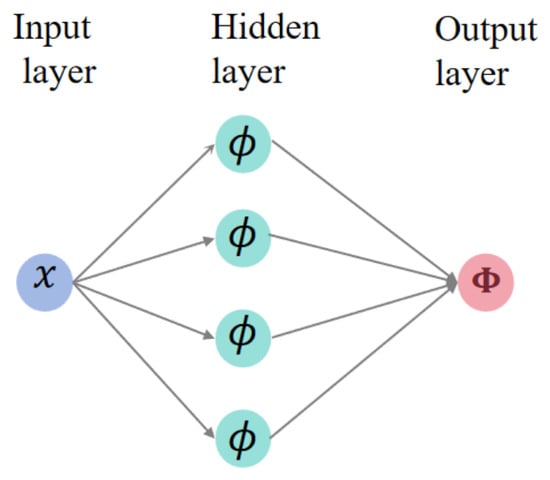
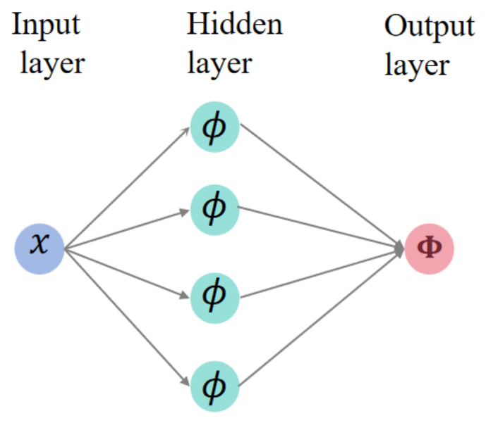
where $\varphi (·)$ is a radial basis function, $\mathit{c}=({\mathbf{c}}_1,\dots ,{\mathbf{c}}_N)$, $\mathit{d}=(d_1,\dots ,d_N)$, and $\mathit{w}=(w_1,\dots ,w_N)$ denote the centers, shape parameters, and weights of the basis functions, respectively, and N is the number of basis functions. We choose the Gaussian function as the basis function in this paper. It possesses a favorable local approximation property: its value decays rapidly to nearly zero away from the center. The centers, shape parameters, and weights of the basis functions are trainable. Figure 1 depicts an RBF network comprising four basis functions.

Figure 1. The architecture of the radial basis function neural network with four neurons.

Next, we denote $\mathrm{\Phi }(\mathit{x};\mathit{w},\mathit{c},\mathit{d})$ simply as $\mathrm{\Phi }$ and incorporate it as a feature embedding into the PINN; in other words, we have

$$\begin{array}{cc}\hfill \tilde{u}(\mathit{x},t,\mathrm{\Phi };\theta )& =W^{\left[L\right]}\sigma (W^{[L-1]}\sigma (\dots \sigma (W^{\left[0\right]}\left[\mathit{x}\right|t\left|\mathrm{\Phi }(\mathit{x};\mathit{w},\mathit{c},\mathit{d})\right]+b^{\left[0\right]})\dots )+b^{[L-1]})+b^{\left[L\right]},\hfill \\ \hfill & =\mathcal{N}\left(\right[\mathit{x}\left|t\right|\mathrm{\Phi }(\mathit{x};\mathit{w},\mathit{c},\mathit{d})];\theta )\hfill \end{array}$$

(10)

where $\theta =\{W^{\left[0\right]},b^{\left[0\right]},\dots ,W^{\left[L\right]},b^{\left[L\right]},\mathit{w},\mathit{c},\mathit{d}\}$ denotes the trainable parameters, $\mathcal{N}$ represents the neural network model, and $\left[\mathbf{x}\right|t\left|\mathrm{\Phi }\right(\mathit{x};\mathit{w},\mathit{c},\mathit{d}\left)\right]$ indicates the column-wise concatenation of these three elements. Due to the learnable shape parameters $\mathit{d}$, the RBF embedding $\mathrm{\Phi }$ can better capture high-frequency features near phase interfaces, thereby improving the PINN’s accuracy.

3.2. Temporal Feature Enhancement: Initial Condition Feature Embedding

To fully utilize the information of the initial condition, we not only impose it as a physical constraint in the loss function but also incorporate it as an additional feature input to the PINN. This enables the network to retain the initial solution information throughout the subsequent evolution, thereby accelerating convergence. The embedded representation is given by

$$\tilde{u}(\mathit{x},t,\mathrm{\Phi },u_0;\theta )=\mathcal{N}\left(\left[\mathit{x}\right|t\left|\mathrm{\Phi }(\mathit{x};\mathit{w},\mathit{c},\mathit{d})\right|u_0\left(\mathit{x}\right)];\theta \right),$$

(11)

where $\mathcal{N}$ represents the neural network model, $\theta =\{W^{\left[0\right]},b^{\left[0\right]},\dots ,W^{\left[L\right]},b^{\left[L\right]},\mathit{w},\mathit{c},\mathit{d}\}$ denotes all trainable parameters, including those of the neural network and the RBF embedding, and $u_0$ is the initial condition function. This design incorporates the initial condition directly as an input feature, establishing an explicit link between the solution at any time and the initial state, thus anchoring the temporal evolution to the initial condition.

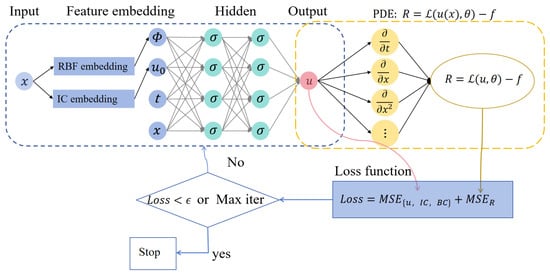
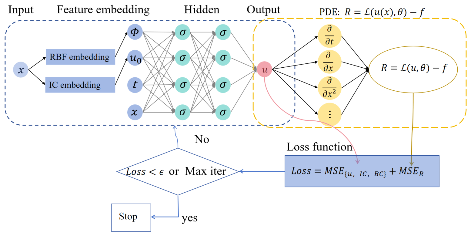
In this paper, we denote the PINN integrating spatial RBF feature embedding and temporal initial condition feature embedding as STFE-PINN. Figure 2 illustrates the architecture of the proposed spatiotemporal feature embedding physics-informed neural network. Given the spatial coordinates $\mathit{x}$, the RBF feature embedding $\mathrm{\Phi }\left(\mathit{x}\right)$ and the initial condition feature embedding (abbreviated as IC embedding) are computed first. Subsequently, $\mathrm{\Phi }\left(\mathit{x}\right)$, the IC embedding, and the spatiotemporal coordinates $(\mathit{x},t)$ are fed together into the PINN to produce the final prediction. The training terminates when the loss falls below a predefined tolerance $ϵ$ or the maximum number of iterations is reached.

Figure 2. Schematic of the spatiotemporal feature embedding physics-informed neural network (STFE-PINN). The spatial coordinates $\mathit{x}$ are used to compute the RBF feature embedding $\mathrm{\Phi }\left(\mathit{x}\right)$ and the initial condition embedding (IC embedding) $u_0\left(\mathit{x}\right)$; these are then fed together with $(\mathit{x},t)$ into the PINN to produce the prediction.

The combination of spatial RBF embedding and temporal initial condition embedding is motivated by their distinct yet complementary roles in resolving phase field dynamics. Physically, the Allen–Cahn equation describes the evolution of diffuse interfaces driven by free energy minimization. The spatial RBF embedding provides a set of locally supported basis functions that can adaptively concentrate near the moving interface, efficiently capturing sharp spatial gradients. The temporal initial condition embedding, on the other hand, injects the initial configuration directly into the network input, acting as a temporally persistent anchor that helps the network maintain the correct phase structure over long time horizons. Practically, the synergistic effect of these two embeddings enables the network to simultaneously resolve fine spatial features and preserve temporal coherence, which is important for long-time simulations of interface dynamics.

3.3. Temporal Domain Decomposition

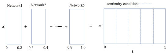
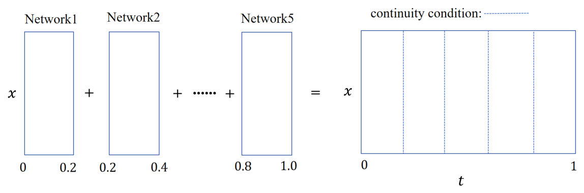
Adaptive sampling in the temporal domain is a highly effective strategy, particularly for phase field models like the Allen–Cahn equation, whose dynamics involve slowly evolving interfaces after rapid transient phases. Training a single PINN across a long temporal horizon often leads to optimization difficulties and uncontrolled error propagation. To circumvent this, we adopt a temporal domain decomposition approach [22]. In our implementation, we partition the entire time horizon into a sequence of subintervals, as illustrated in Figure 3. The time interval $[0,T]$ is divided into $N_T$ equal subintervals of a length $\mathrm{\Delta }t=T/N_T$, and a separate STFE-PINN with the same architecture but independently trainable parameters is assigned to each. The training proceeded sequentially; we first trained the network for the first subinterval until convergence and then froze its parameters. Subsequently, the second subinterval was trained, and this process was repeated until all $N_T$ subintervals were processed. Let ${\tilde{u}}^{\left(k\right)}(\mathit{x},t)$ denote the solution on the kth subinterval. The first subinterval is initialized with the prescribed $u_0\left(\mathit{x}\right)$. For $k\ge 2$, the initial condition of the kth subinterval is taken as the predicted solution at the final time of the $(k-1)$th subinterval, which is evaluated using the frozen network of the preceding interval. To ensure smooth transition between subintervals, we enforced not only the continuity of the solution value but also the continuity of its time derivative, which avoided slope jumps at the interval interfaces and further improved the smoothness of long-time simulations:

$$\begin{array}{cc}\hfill {\tilde{u}}^{\left(k\right)}(\mathit{x},T_k)& ={\tilde{u}}^{(k-1)}(\mathit{x},T_k),k=2,3,\dots ,N_T\hfill \end{array}$$

(12)

$$\begin{array}{cc}\hfill {\partial }_t{\tilde{u}}^{\left(k\right)}(\mathit{x},T_k)& ={\partial }_t{\tilde{u}}^{(k-1)}(\mathit{x},T_k),k=2,3,\dots ,N_T\hfill \end{array}$$

(13)

where $T_k$ denotes the endpoint of the kth subinterval and $N_T$ denotes the number of subintervals.

Figure 3. Temporal domain decomposition with sequential training. The time domain $[0,1]$ is partitioned into five equal subintervals, each handled by a separate neural network with an identical architecture. Training proceeds subinterval by subinterval, with the parameters of earlier subintervals frozen after convergence; dashed lines indicate continuity conditions.

Accordingly, the original loss function in Equation (8) is modified as follows. For the first subinterval $k=1$, the loss remains identical to Equation (8), imposing the given initial condition $u_0\left(\mathit{x}\right)$. For subsequent subintervals $k\ge 2$, the initial condition is replaced by the continuity conditions in Equations (12) and (13), yielding

$$\begin{array}{cc}\hfill Loss\left({\theta }_k\right)=& {\displaystyle \frac{1}{N_r}}{\displaystyle \sum _{i=1}^{N_r}}{\left(\mathcal{L}{\tilde{u}}^{\left(k\right)}({\mathit{x}}_r^i,t_r^i;{\theta }_k)-f({\mathit{x}}_r^i,t_r^i)\right)}^2\hfill \\ \hfill & +{\displaystyle \frac{{\lambda }_b}{N_b}}{\displaystyle \sum _{j=1}^{N_b}}{\left(\mathcal{B}{\tilde{u}}^{\left(k\right)}({\mathit{x}}_b^j,t_b^j;{\theta }_k)-g({\mathit{x}}_b^j,t_b^j)\right)}^2\hfill \\ \hfill & +{\displaystyle \frac{{\lambda }_0}{N_0}}{\displaystyle \sum _{l=1}^{N_0}}{\left({\tilde{u}}^{\left(k\right)}({\mathit{x}}_0^l,T_{k-1};{\theta }_k)-{\tilde{u}}^{(k-1)}({\mathit{x}}_0^l,T_{k-1})\right)}^2\hfill \\ \hfill & +{\displaystyle \frac{{\lambda }_0}{N_0}}{\displaystyle \sum _{l=1}^{N_0}}{\left({\partial }_t{\tilde{u}}^{\left(k\right)}({\mathit{x}}_0^l,T_{k-1};{\theta }_k)-{\partial }_t{\tilde{u}}^{(k-1)}({\mathit{x}}_0^l,T_{k-1})\right)}^2,\hfill \end{array}$$

(14)

where ${\theta }_k$ denotes the trainable parameters of the kth subnetwork; $N_r$, $N_b$, and $N_0$ are the numbers of interior, boundary, and initial collocation points for the kth subinterval, respectively, with corresponding point sets ${\left\{({\mathit{x}}_r^i,t_r^i)\right\}}_{i=1}^{N_r}$, ${\left\{({\mathit{x}}_b^j,t_b^j)\right\}}_{j=1}^{N_b}$, and ${\left\{{\mathit{x}}_0^l\right\}}_{l=1}^{N_0}$; ${\lambda }_b$ and ${\lambda }_0$ are penalty coefficients; and ${\tilde{u}}^{(k-1)}$ and ${\partial }_t{\tilde{u}}^{(k-1)}$ denote the solution and its time derivative from the frozen $(k-1)$th subnetwork, respectively, evaluated at the interface $t=T_{k-1}$.

This sequential decomposition effectively mitigates the gradient magnitude imbalance caused by long-time integration and allows the network to concentrate on local dynamical features, thereby substantially improving the accuracy in resolving abrupt interfacial changes.

4. Numerical Experiments

We conducted a series of numerical experiments in one, two, and three spatial dimensions to assess the convergence and stability of the proposed STFE-PINN. The accuracy was quantified by the relative $L^2$ error between the STFE-PINN solution $\tilde{u}$ and a reference solution $u_r$ obtained from the classical numerical methods with high accuracy (or from an analytic solution, if one existed):

$$\mathrm{error}={\displaystyle \frac{\sqrt{{\sum }_{i=1}^n{\left|\tilde{u}({\mathit{x}}_i,t_i)-u_r({\mathit{x}}_i,t_i)\right|}^2}}{\sqrt{{\sum }_{i=1}^n{\left|u_r({\mathit{x}}_i,t_i)\right|}^2}}},$$

(15)

where ${\left\{({\mathit{x}}_i,t_i)\right\}}_{i=1}^n$ are the test grid points.

For all one-dimensional examples, unless otherwise stated, the examples were considered for the Allen–Cahn equation (Equation (1)) with a polynomial potential. The initial learning rate was 0.001, decaying by a factor of 0.1 every 100 epochs to a minimum of 0.00001. For the interior domain, the collocation points were uniformly sampled with a temporal step size of 0.01 and a spatial step size of 0.01. Boundary points were sampled with a step size of 0.01, and initial points with a step size of 0.002. The relative error was evaluated on an equidistant 201 × 201 spatiotemporal grid. The batch size was 64, the maximum number of iterations was 500, the number of temporal subdomains $N_T$ was set to 1 by default, the penalty coefficient for the boundary condition was 1.0, and that for initial condition was 500.0. The network consisted of 5 hidden layers with 64 neurons each and the tanh activation function. The radial basis functions were chosen as Gaussians. The number of RBFs was set to 500, with their centers uniformly distributed over the spatial domain. The RBF weights were initialized from a standard normal distribution, and the shape parameters were drawn from a uniform distribution on $(0,10)$. The parameters of the PINN were initialized using the Xavier uniform initialization scheme. All experiments were conducted on a workstation equipped with an Intel Core Ultra 7 265K CPU, 64 GB of DDR5 RAM, and an NVIDIA GeForce RTX 4090 GPU.

4.1. Comparative Study for the 1D Allen–Cahn Equation

Consider the classical Allen–Cahn equation (Equation (1)), which in one spatial dimension takes the explicit form

$${\displaystyle \frac{\partial u}{\partial t}}=\mu \left({\epsilon }^2{\displaystyle \frac{{\partial }^{2}u}{\partial x^2}}-(u^3-u)\right),x\in [-1,1],t\in (0,1],$$

(16)

with parameters ${\epsilon }^2=0.0001$ and $\mu =5$. The periodic boundary conditions are

$$u(-1,t)=u(1,t),{\displaystyle \frac{\partial u}{\partial x}}(-1,t)={\displaystyle \frac{\partial u}{\partial x}}(1,t),$$

(17)

and, as in [37], the chosen initial condition was

$$u(x,0)=x^{2}cos\left(\pi x\right),x\in [-1,1].$$

(18)

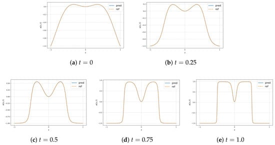
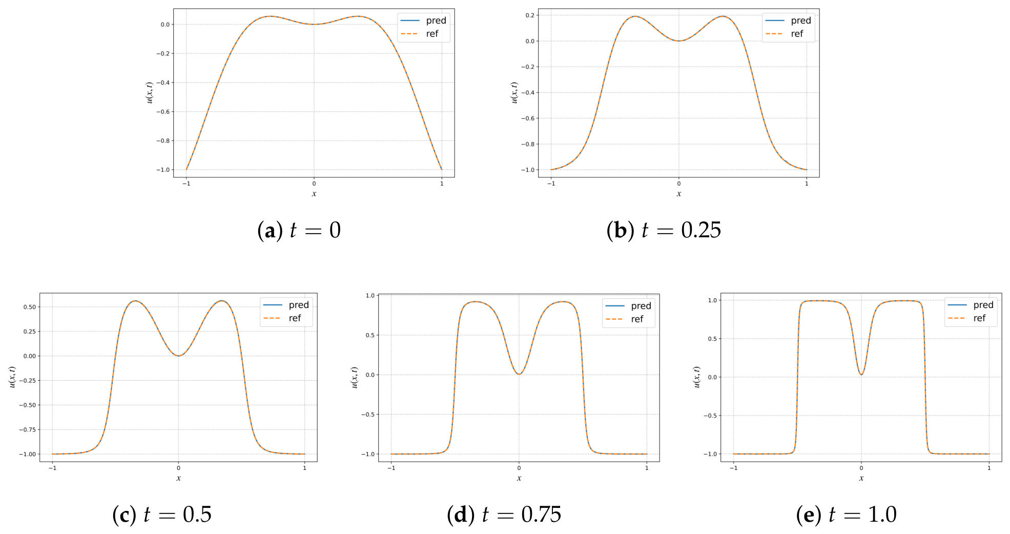
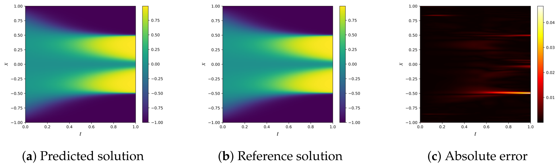
Figure 4 compares the predicted solution (STFE-PINN) with the reference solution at different time instants ($t=0,0.25,0.5,0.75,1.0$). As time evolved, the solution became increasingly oscillatory. At the final time $t=1$, most other PINN variants [31,38,39] exhibited large errors concentrated near $x=0$; in contrast, our method achieved excellent agreement, as demonstrated in Figure 4. Furthermore, Figure 5 presents the predicted solution, the reference solution, and the absolute error over the entire domain. It can be observed that the relatively large errors were primarily located in regions where the phase interface underwent sharp changes.

Figure 4. Section 4.1: Comparison between predicted and reference solution profiles at $t=0,0.25,0.5,0.75,1.0$.

Figure 5. Section 4.1: Predicted solution, reference solution, and absolute pointwise error over the spacetime domain.

In Table 1, we compare the proposed STFE-PINN with various PINN variants. To ensure a fair comparison, the reference solution used to compute all relative $L^2$ errors was taken from [31].The errors for the comparison methods (std-PINN, XPINN, bc-PINN, bc-PINN + logresidual, bc-PINN + ICGL + TL, ACP, AT + ACP, and AT + ACP + Energy Penalty) were directly cited from their respective original papers, where they were evaluated against this same reference solution. For our STFE-PINN, we computed the error on an identical test grid and the same reference solution as that used in [31] so that all results were fully comparable. Specifically, the results for std-PINN [14], XPINN [38], bc-PINN [39], bc-PINN + logresidual [39], and bc-PINN + ICGL + TL [39] were obtained with four hidden layers, 200 neurons per layer, 512 initial points, 201 boundary points, and 20,000 collocation points per time segment. The results for ACP [22] and AT + ACP [31] were obtained with four hidden layers, 128 neurons per layer, 512 initial points, 200 boundary points, and 10,000 collocation points. The results for AT + ACP + Energy Penalty [31] were obtained with four hidden layers, 100 neurons per layer, 500 initial points, 48 boundary points, and 500 collocation points. Notably, our STFE-PINN used only five hidden layers with 64 neurons and 500 radial basis functions, resulting in fewer parameters than the standard PINN and its variants, yet it still achieved the optimal performance among all methods, as summarized in Table 1.

Table 1. Comparison of relative $L^2$ errors for the Section 4.1.

Method	Relative ${\mathit{L}}^2$ Error
std-PINN [14]	0.9919
XPINN [38]	0.9612
bc-PINN [39]	0.0701
bc-PINN + logresidual [39]	0.0300
ACP [22]	0.0233
bc-PINN + ICGL + TL [39]	0.0168
AT + ACP [31]	0.0078
AT + ACP + Energy Penalty [31]	0.0053
STFE-PINN (ours)	0.0031

4.2. Ablation Study for the Traveling Wave Problem

To quantitatively assess the contribution of each proposed component, we evaluated the effects of the spatial RBF embedding and the temporal initial condition embedding separately. Specifically, we considered a traveling wave problem [40] for the 1D Allen–Cahn equation, for which the analytical solution served as the reference for error quantification. Ablation experiments were conducted by removing one embedding at a time from the full model and comparing the resulting prediction accuracy. The results confirm that both the spatial RBF embedding and the temporal initial condition embedding played essential roles in improving the solution quality, and their combination yielded the most accurate and stable approximations.

The traveling wave solution [40] is given by

$$\begin{array}{c}\hfill u_{\mathrm{exact}}(x,t)={\displaystyle \frac{1}{2}}\left[1-tanh\left({\displaystyle \frac{x-3t/\left(\sqrt{2}\epsilon \right)}{2\sqrt{2}\epsilon }}\right)\right],\end{array}$$

(19)

which satisfies the following one-dimensional Allen–Cahn equation on an infinite domain:

$$\begin{array}{c}\hfill {\displaystyle \frac{\partial u(x,t)}{\partial t}}=-{\displaystyle \frac{F_u^{\prime }\left(u(x,t)\right)}{{\epsilon }^2}}+{\displaystyle \frac{{\partial }^{2}u(x,t)}{\partial x^2}},x\in \mathrm{\Omega }=(-\infty ,\infty ),t>0.\end{array}$$

(20)

Note that this form was obtained from Equation (1) by rescaling time as $t\leftarrow {\epsilon }^{2}t$; this is equivalent to the standard Allen–Cahn equation under a different time scale.

In the numerical simulations, the domain was truncated to a finite domain $\mathrm{\Omega }=(L_x,R_x)$ with $\epsilon =0.1,L_x=-2,R_x=5$ and $T=\sqrt{\epsilon }$. The homogeneous Neumann boundary condition was imposed. The rationale behind this boundary condition is as follows. The first derivative of the exact solution in Equation (19) is given by

$${\displaystyle \frac{\partial u_{\mathrm{exact}}}{\partial x}}(x,t)=-{\displaystyle \frac{1}{4\sqrt{2\epsilon }}}{sech}^2\left({\displaystyle \frac{x-3t/\left(\sqrt{2}\epsilon \right)}{2\sqrt{2}\epsilon }}\right),$$

(21)

which is strictly negative for all x. However, when the transition layer is sufficiently far from the domain boundaries, the first derivatives at the boundary points, $\partial u(L_x,t)/\partial x$ and $\partial u(R_x,t)/\partial x$, are close to zero. Hence, the homogeneous Neumann boundary condition provides a good approximation for the Allen–Cahn equation in this setting.

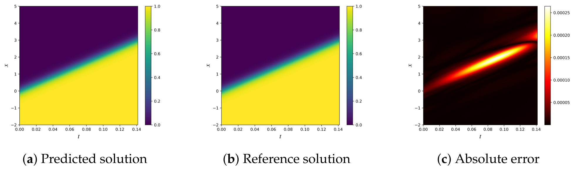
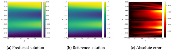
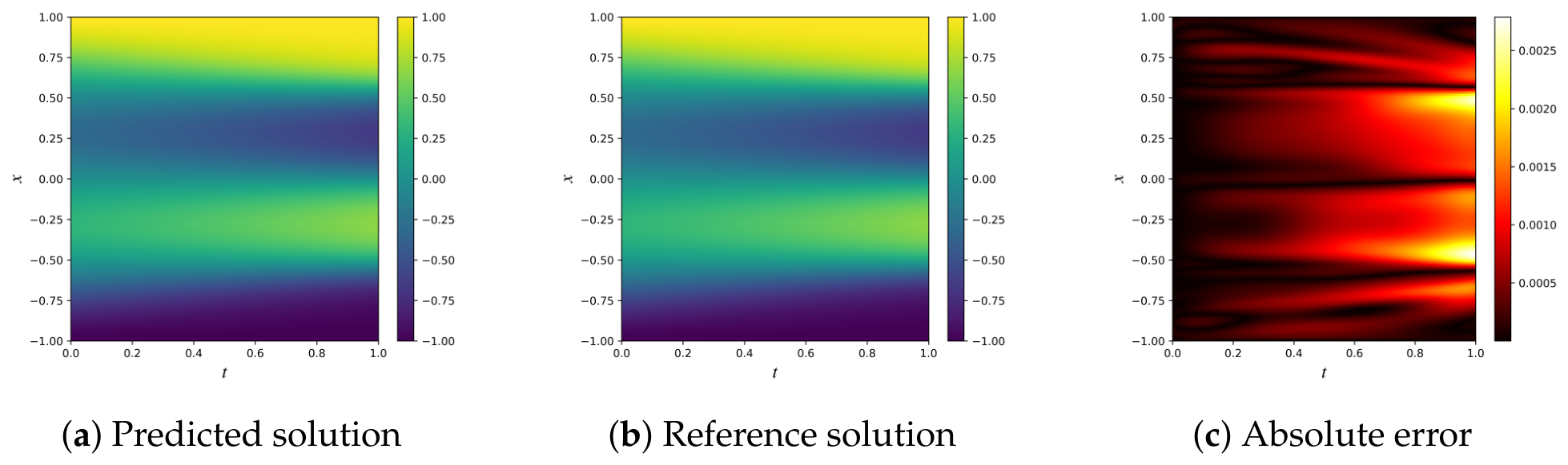
Figure 6 shows the predicted solution from the STFE-PINN model, the exact solution, and the pointwise absolute error. Large errors were concentrated near the sharp interface, yet they remained at a remarkably low order of ${10}^{-4}$. Thus, the STFE-PINN achieved high accuracy for the traveling wave problem.

Figure 6. Section 4.2: Predicted solution, reference solution, and absolute pointwise error for the traveling wave problem.

In the following, we describe the four ablation configurations designed to evaluate the individual roles of the spatial RBF embedding and the temporal initial condition embedding for the traveling wave problem:

• PINN: Standard PINN without any feature embedding.
• PINN + RBF: PINN with spatial RBF feature embedding.
• PINN + Initial: PINN with temporal initial condition feature embedding.
• PINN + RBF + Initial (STFE-PINN): Combination of both spatial RBF and temporal initial condition embeddings.

All ablation experiments were conducted under identical conditions, including the same set of training and test collocation points, the same hyperparameter settings, and the same configuration of the PINN model (network architecture, activation functions, and optimization details).

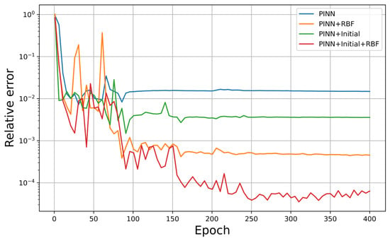
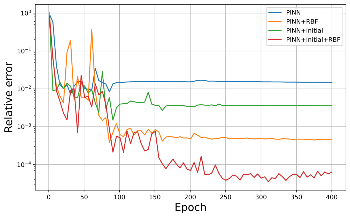
Figure 7 plots the relative $L^2$ error versus iterations for the four configurations. The standard PINN converged slowly and saturated at a relatively high error level (the order of ${10}^{-2}$). Adding either RBF embedding or initial condition embedding enhanced the accuracy. Moreover, as shown in the figure, the inclusion of initial condition embedding enabled the relative error to decrease more rapidly to the order of ${10}^{-2}$, which demonstrates that initial condition embedding not only improved the accuracy of the PINN but also accelerated its convergence. The STFE-PINN (PINN + RBF + Initial) achieved the lowest error (the order of ${10}^{-5}$), demonstrating the synergistic effect of the two feature embeddings.

Figure 7. Section 4.2: Convergence of the relative $L^2$ error for four ablation experiments under identical training conditions.

Table 2 reports the final relative $L^2$ error, number of trainable parameters, and average training time per epoch for each configuration. From the Table 2, we observe that both the RBF embedding and the initial condition embedding individually improved the accuracy over the standard PINN, while their combination (STFE-PINN) reduced the error by three orders of magnitude. Notably, the full model achieved this substantial accuracy gain with a modest increase in parameters and training time. These results confirm the effectiveness of the proposed spatial–temporal feature embeddings.

Table 2. Ablation study results for Section 4.2.

Configuration	Relative ${\mathit{L}}^2$ Error	Parameters	Training Time (s)
PINN	$1.48\times {10}^{-2}$	12,737	4.40
PINN + RBF	$4.54\times {10}^{-4}$	14,301	5.64
PINN + Initial	$3.57\times {10}^{-3}$	12,801	4.99
PINN + RBF + Initial	$6.30\times {10}^{-5}$	14,365	5.88

To further analyze the sensitivity of the Gaussian RBF embedding, we conducted a combined ablation study on the number of RBF basis functions N and the initialization range of the shape parameter $\mathit{d}$. Five configurations were compared: $N=300$ with $\mathit{d}\in [0,1]$, $N=300$ with $\mathit{d}\in [0,10]$, $N=300$ with $\mathit{d}\in [0,20]$, $N=50$ with $d\in [0,10]$, and $N=1000$ with $\mathit{d}\in [0,10]$. All other settings (network architecture, learning rate, optimizer, etc.) were kept identical to those used in the full STFE-PINN model. Table 3 reports the relative $L^2$ error for each configuration.The configuration with $N=300$ and $\mathit{d}\in [0,10]$ achieved the optimal performance, with an error to the order of ${10}^{-5}$, while the errors for the other four configurations were to the order of ${10}^{-3}$.This indicates that although an improper number of basis functions or an unsuitable initialization range for the shape parameters degraded the accuracy, the method remained convergent in all tested cases.

Table 3. Ablation study of the STFE-PINN on the number of RBF basis functions and the initialization range of the shape parameters.

Configuration	Relative ${\mathit{L}}^2$ Error
$N=300$, $\mathit{d}\in [0,1]$	$2.72\times {10}^{-3}$
$N=300$, $\mathit{d}\in [0,10]$	$6.30\times {10}^{-5}$
$N=300$, $\mathit{d}\in [0,20]$	$2.28\times {10}^{-3}$
$N=50$, $\mathit{d}\in [0,10]$	$2.43\times {10}^{-3}$
$N=1000$, $\mathit{d}\in [0,10]$	$3.56\times {10}^{-3}$

4.3. 1D Allen–Cahn Equation: Energy Dissipation and Maximum Bound Principle

We further examined the capability of the STFE-PINN method in capturing the fundamental mathematical properties of the Allen–Cahn equation (Equation (1)). Specifically, we designed a numerical experiment to simultaneously test the energy dissipation law and the maximum bound principle. To this end, we considered the domain $(x,t)\in [-1,1]\times [0,1]$ with parameters ${\epsilon }^2=0.0001$ and $\mu =1.0$. Dirichlet boundary conditions were imposed, given by

$$u(-1,t)=-1,u(1,t)=1.$$

(22)

The initial condition was a smooth, non-symmetric profile whose magnitude was bounded by one, given by

$$u(x,0)=0.53x+0.47sin(-1.5\pi x),x\in [-1,1],$$

(23)

which evolved into a complex interface structure.

Figure 8 compares the predicted solution with the reference solution over the entire spatiotemporal domain. Large errors were primarily concentrated in regions where the phase field underwent sharp variations; nevertheless, the predicted solution closely matched the reference solution, with an absolute pointwise error to the order of ${10}^{-3}$.

Figure 8. Section 4.3: Predicted solution, reference solution, and absolute pointwise error over the entire domain.

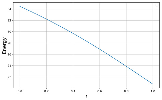
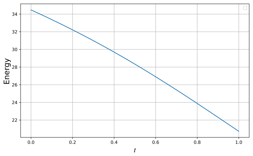
We now examine the two key mathematical properties. First, Figure 9 shows the evolution of the total free energy $E\left(u\right(t\left)\right)$ defined in Equation (4), computed via its discrete form on a uniform $201\times 201$ grid. As expected from the gradient flow property of the Allen–Cahn equation, the energy decreased monotonically with time, confirming that the STFE-PINN prediction respects the energy dissipation law.

Figure 9. Section 4.3: Time evolution of the total free energy $E\left(u\right(t\left)\right)$ defined in Equation (4).

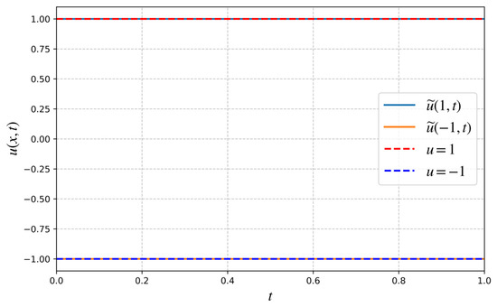
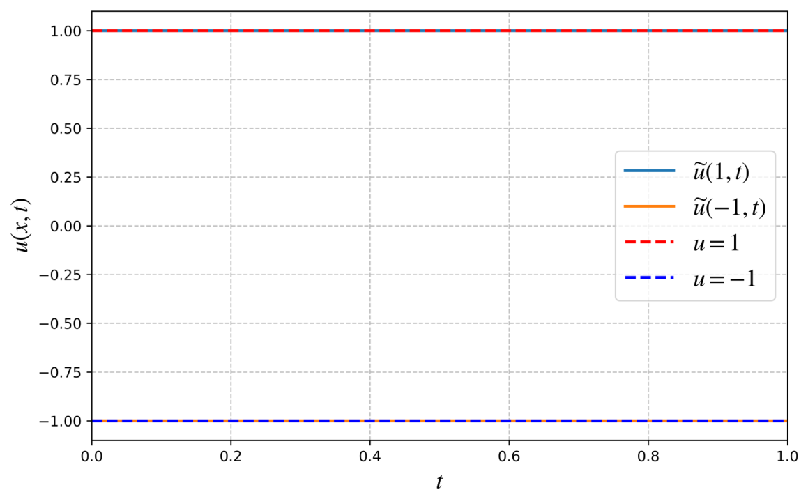
Second, the Dirichlet boundary conditions in this problem satisfied $-1\le u\le 1$ at the boundaries, and the maximum bound principle dictated that the solution had to remain within this range for all times if the initial condition did. As shown in Figure 8a, the predicted solution attained its maximum at $x=1$ and its minimum at $x=-1$. To examine the adherence to the bounds more closely, we present a direct comparison of the predicted solution at $x=1$ and $x=-1$ with the respective constant boundary values 1 and $-1$ in Figure 10. It can be seen that the absolute value of the predicted extremum was confined within 1, providing numerical evidence that the STFE-PINN method also respects the maximum bound principle.

Figure 10. Comparison of the predicted solution $\tilde{u}$ with the constant bounds 1 and $-1$ at $x=1$ and $x=-1$. The horizontal dashed lines denote the bounds, while the solid curves show the predicted solution at the two endpoints as functions of time.

4.4. 2D Allen–Cahn Equation

We consider the two-dimensional Allen–Cahn equation (Equation (1)) on the domain $(x,y,t)\in [-1,1]\times [-1,1]\times [0,1]$, with parameters ${\epsilon }^2=0.0001$ and $\mu =5$. The exact solution was taken as $u_{\mathrm{exact}}(x,y,t)=e^{-2{\epsilon }^{2}t}sin(x+y)$. Substituting this expression into Equation (1) yields the source term

$$\begin{array}{c}\hfill g(x,y,t)=5\left(e^{-6{\epsilon }^{2}t}{sin}^3(x+y)-e^{-2{\epsilon }^{2}t}sin(x+y)\right),\end{array}$$

(24)

together with the initial condition $u_0(x,y)=sin(x+y)$ and the Dirichlet boundary condition.

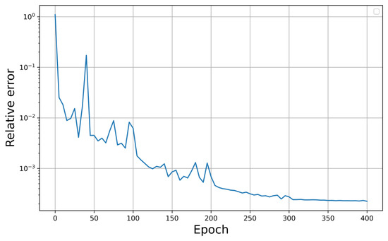
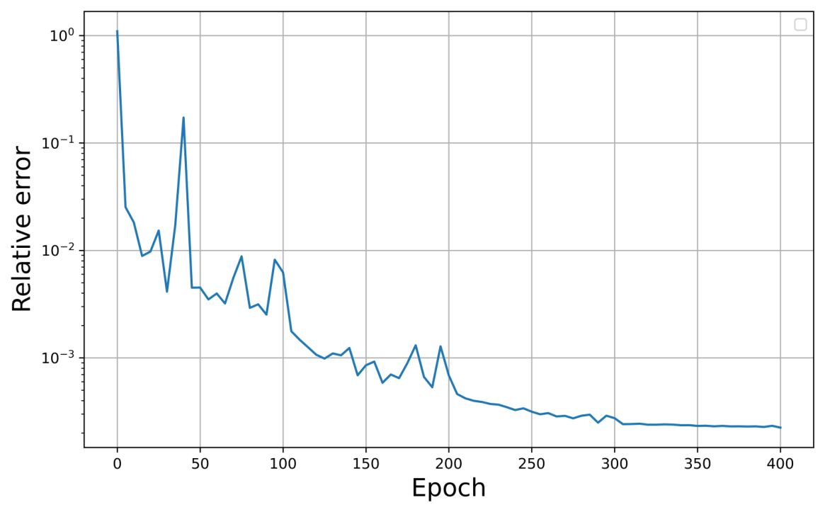
Figure 11 shows the evolution of the relative $L^2$ error over the training. The error decreased rapidly within the first few hundred iterations and converged to the order of ${10}^{-4}$ after about 200 iterations, demonstrating that the STFE-PINN method achieved high accuracy on this two-dimensional Allen–Cahn equation.

Figure 11. Section 4.4: Relative $L^2$ error in terms of iteration for the 2D Allen–Cahn equation.

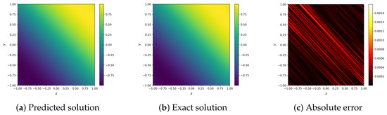
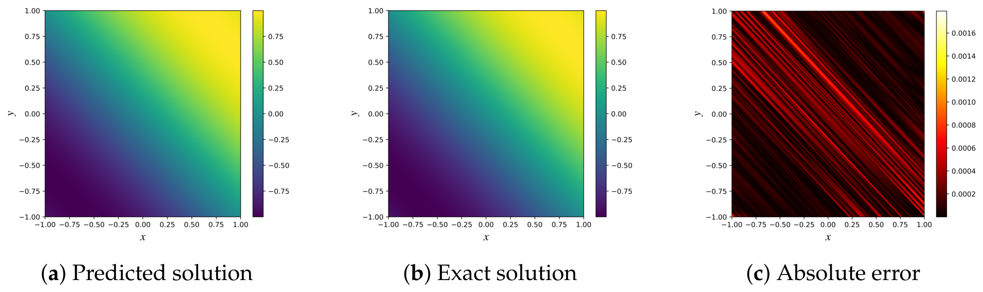
Figure 12 compares the predicted solution, the exact solution, and the absolute pointwise error at the final time $t=1.0$. As shown in the figure, the absolute pointwise error reached the order of ${10}^{-3}$, indicating that our method provided a good approximation to the exact solution.

Figure 12. Section 4.4: Predicted solution, exact solution, and absolute pointwise error at $t=1.0$.

4.5. Single-Drop Shrinking for the 2D Allen–Cahn Equation

We now consider a classical two-dimensional benchmark: the shrinking of a single drop governed by the Allen–Cahn equation (Equation (1)) on $\mathrm{\Omega }={[0,1]}^2$ with homogeneous Neumann boundary conditions [22]:

$$\begin{array}{c}\hfill {\displaystyle \frac{\partial u}{\partial \mathbf{n}}}=0\mathrm{on}\partial \mathrm{\Omega }.\end{array}$$

(25)

The initial condition is a circular interface given by

$$\begin{array}{c}\hfill u(x,y,0)=tanh\left({\displaystyle \frac{0.35-\sqrt{{(x-0.5)}^2+{(y-0.5)}^2}}{2\epsilon }}\right).\end{array}$$

(26)

where $\mu =10$ is the mobility and $\epsilon =0.025$ is the interface width. This example models phase separation with a droplet that gradually shrinks under surface tension and eventually disappears.

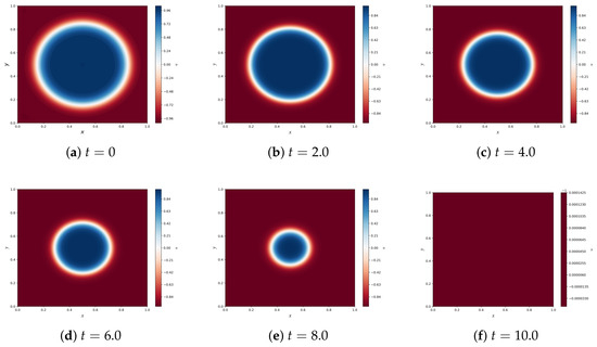
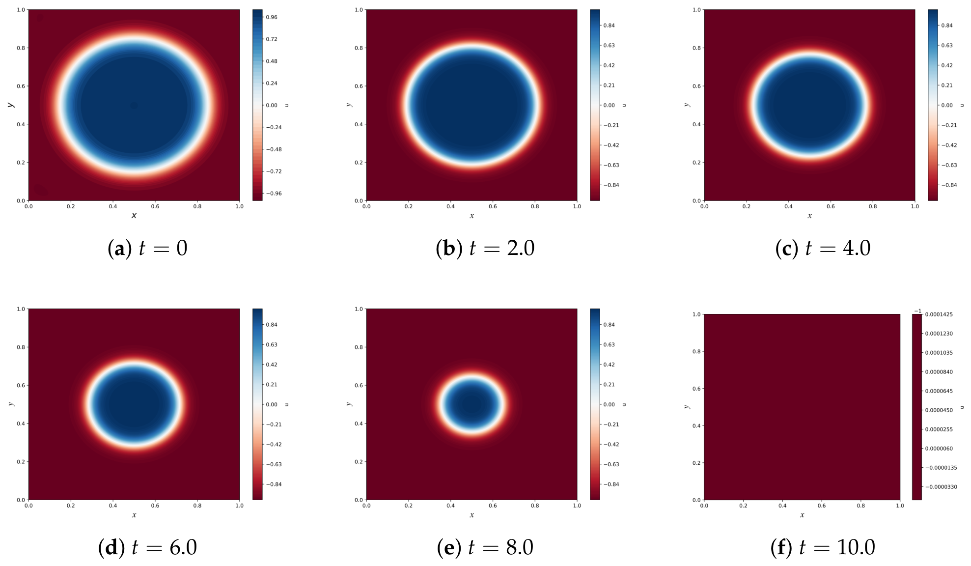
To handle the long time horizon $T=10$, we employed the temporal domain decomposition strategy with $N_T=5$ subintervals, each of a length $\mathrm{\Delta }t=2.0$. For each subinterval, the training data consisted of 500,000 interior collocation points uniformly sampled from the spacetime domain, together with boundary points and initial points; the boundary points were distributed uniformly over the four edges of $\partial \mathrm{\Omega }$ (300 points per edge, giving 1200 boundary points in total), and 800 initial points were uniformly sampled on $\mathrm{\Omega }$ at the initial time of that subinterval. The network was trained with a batch size of 2048, and all other hyperparameters (such as the network architecture, learning rate, and optimizer settings) were kept identical to those used in the one-dimensional examples. The training proceeded sequentially from one subinterval to the next, as described in Figure 3. Figure 13 illustrates the evolution of the predicted solution at $t=0,2,4,6,8,10$. It can be observed that the circular initial interface gradually shrank and eventually disappeared, which is consistent with the numerical results reported in [31]. This consistency confirms that the proposed STFE-PINN successfully captured the phase separation dynamics.

Figure 13. Section 4.5: Predicted solution at $t=0,2,4,6,8,10$ for the single-drop shrinking problem.

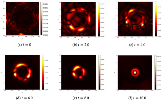
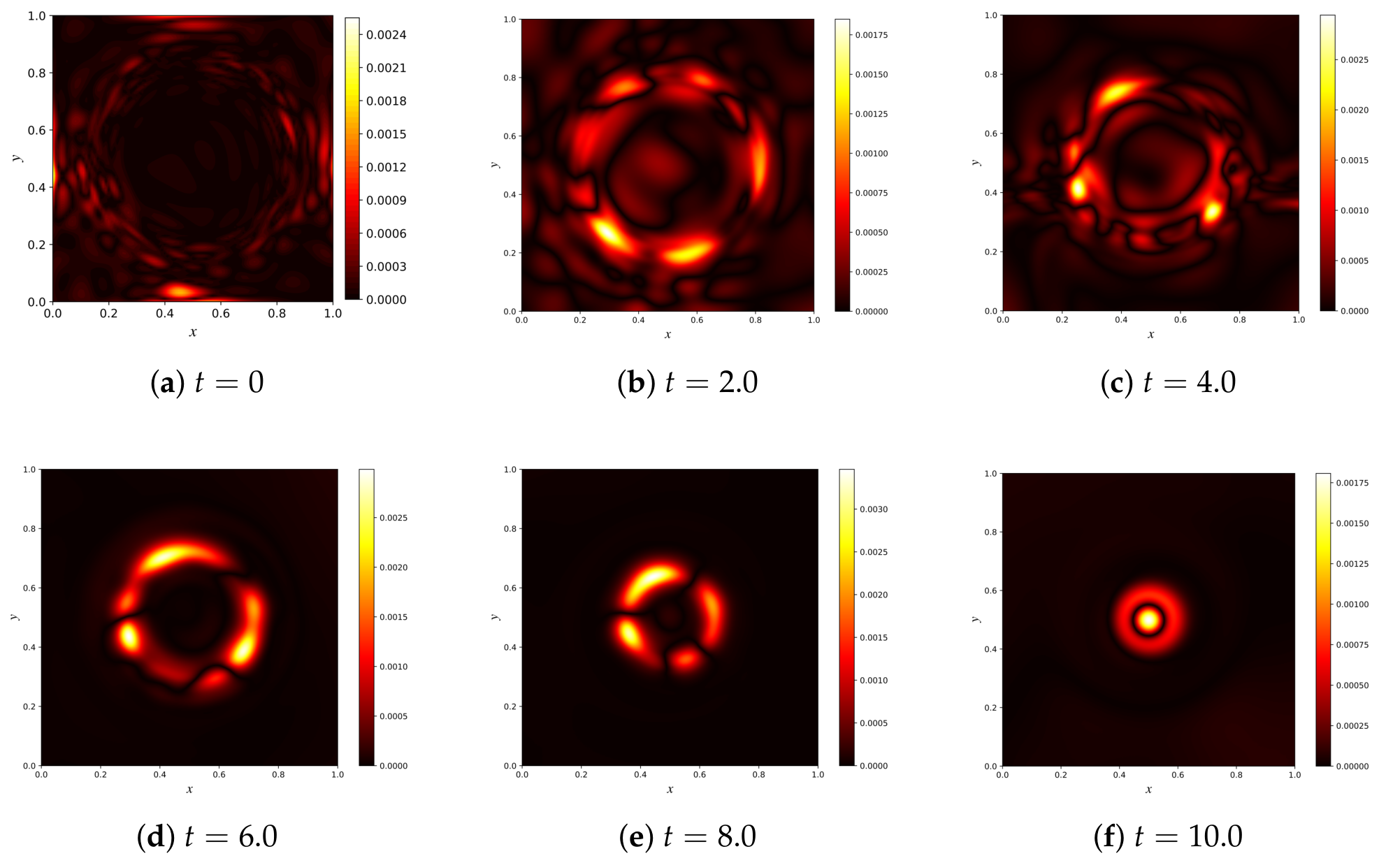
Next, we compare the predicted solution with a high-resolution reference solution obtained by a classical numerical scheme [41]. Figure 14 presents the pointwise absolute errors at six representative time instants $t=0,2,4,6,8,10$. We observe that the absolute errors remained to the order of ${10}^{-3}$ and predominantly localized near the moving interface of the shrinking drop, where the solution underwent sharp spatial transitions. Despite the long time horizon, the error distribution stayed stable without visible accumulation, further confirming the accuracy and robustness of the proposed STFE-PINN.

Figure 14. Section 4.5: Pointwise absolute errors between the STFE-PINN prediction and the reference solution at $t=0,2,4,6,8,10$ for the single-drop shrinking problem.

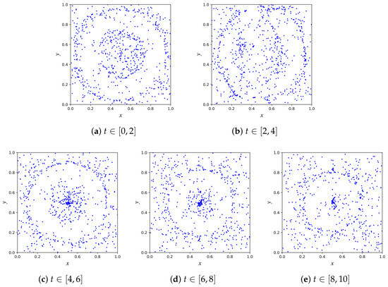
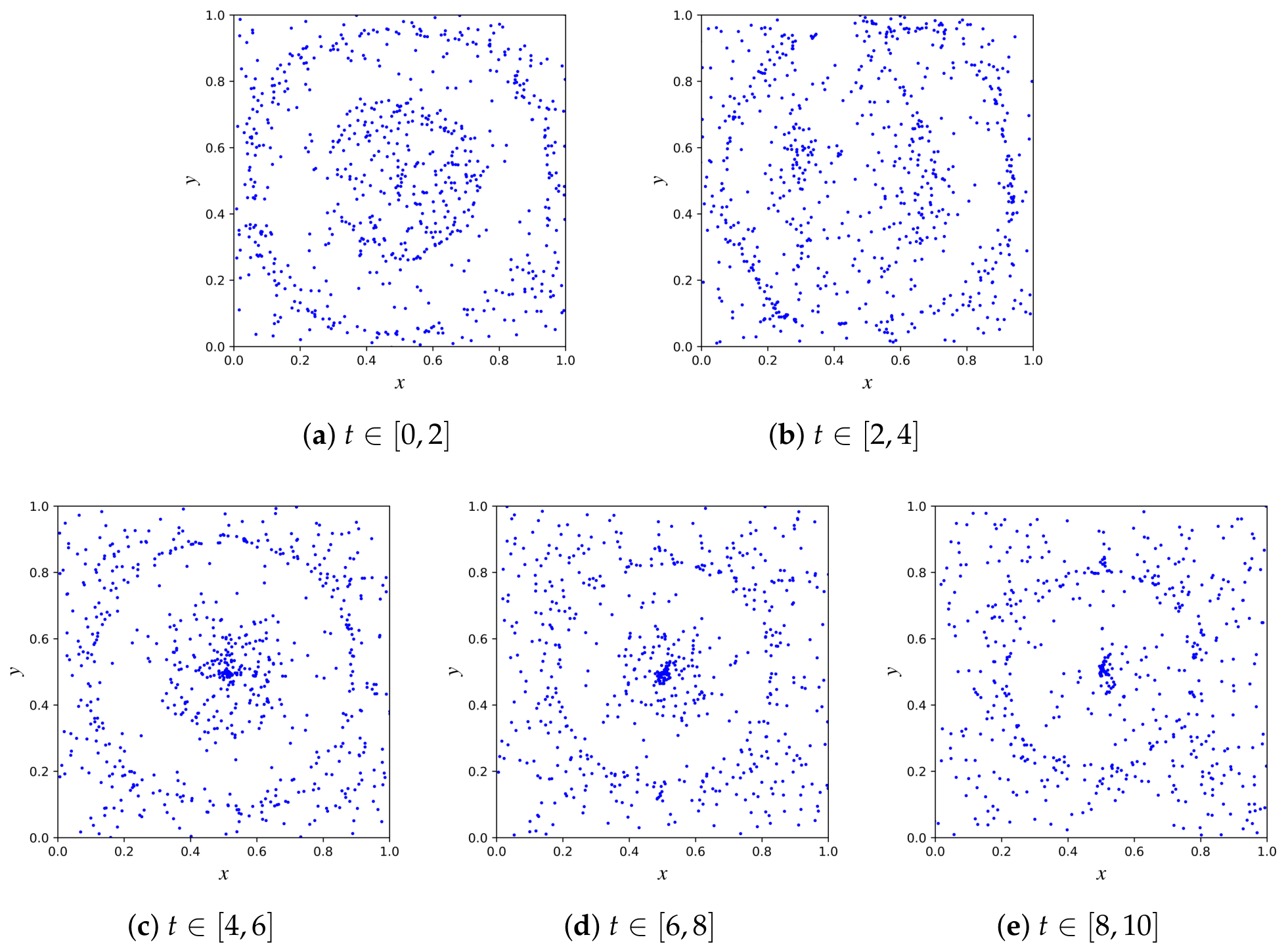
To further assess the interface-capturing capability of the proposed RBF embedding, we visualized the spatial distribution of all Gaussian RBF centers across the five temporal subintervals. Figure 15 shows these centers, and their distribution closely followed the contour of the shrinking droplet interface at each stage, confirming that the RBF embedding automatically concentrated its bases near the sharp interface. This demonstrates the effectiveness of the proposed spatial feature embedding in resolving the steep transitions of the Allen–Cahn equation and provides a direct, interface-specific assessment of the technique.

Figure 15. Distribution of the RBF centers for each temporal subinterval in Section 4.5. The centers concentrated along the moving interface, illustrating the adaptive resolution of sharp gradients by the spatial RBF embedding.

4.6. Single-Drop Shrinking for the 3D Allen–Cahn Equation

Consider a three-dimensional Allen–Cahn equation (Equation (1)) on $\mathrm{\Omega }={[0,1]}^3$ with homogeneous Neumann boundary conditions [31]:

$$\begin{array}{c}\hfill {\displaystyle \frac{\partial u}{\partial \mathbf{n}}}=0\mathrm{on}\partial \mathrm{\Omega }.\end{array}$$

(27)

The initial condition is given by a spherical interface centered at $(0.5,0.5,0.5)$:

$$u(x,y,z,0)=tanh\left({\displaystyle \frac{0.35-\sqrt{{(x-0.5)}^2+{(y-0.5)}^2+{(z-0.5)}^2}}{2\epsilon }}\right).$$

(28)

where $\mu =10$ and $\epsilon =0.05$. This example is analogous to the previous example but extends the configuration to a three-dimensional single drop shrinking.

For this three-dimensional problem, we used 2,000,000 interior collocation points uniformly sampled from the spacetime domain, together with boundary points distributed uniformly over the six faces of $\partial \mathrm{\Omega }$ ($100\times 100$ points per face, i.e., 60,000 boundary points in total) and 1000 initial points uniformly sampled on $\mathrm{\Omega }$ at $t=0$. The network was trained with a batch size of 4096, and all other hyperparameters remained identical to those employed in the two-dimensional examples. Due to the high dimensionality, we assessed the convergence mainly through the loss function and the qualitative properties of the predicted solution, as a high-resolution reference solution was computationally prohibitive.

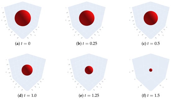
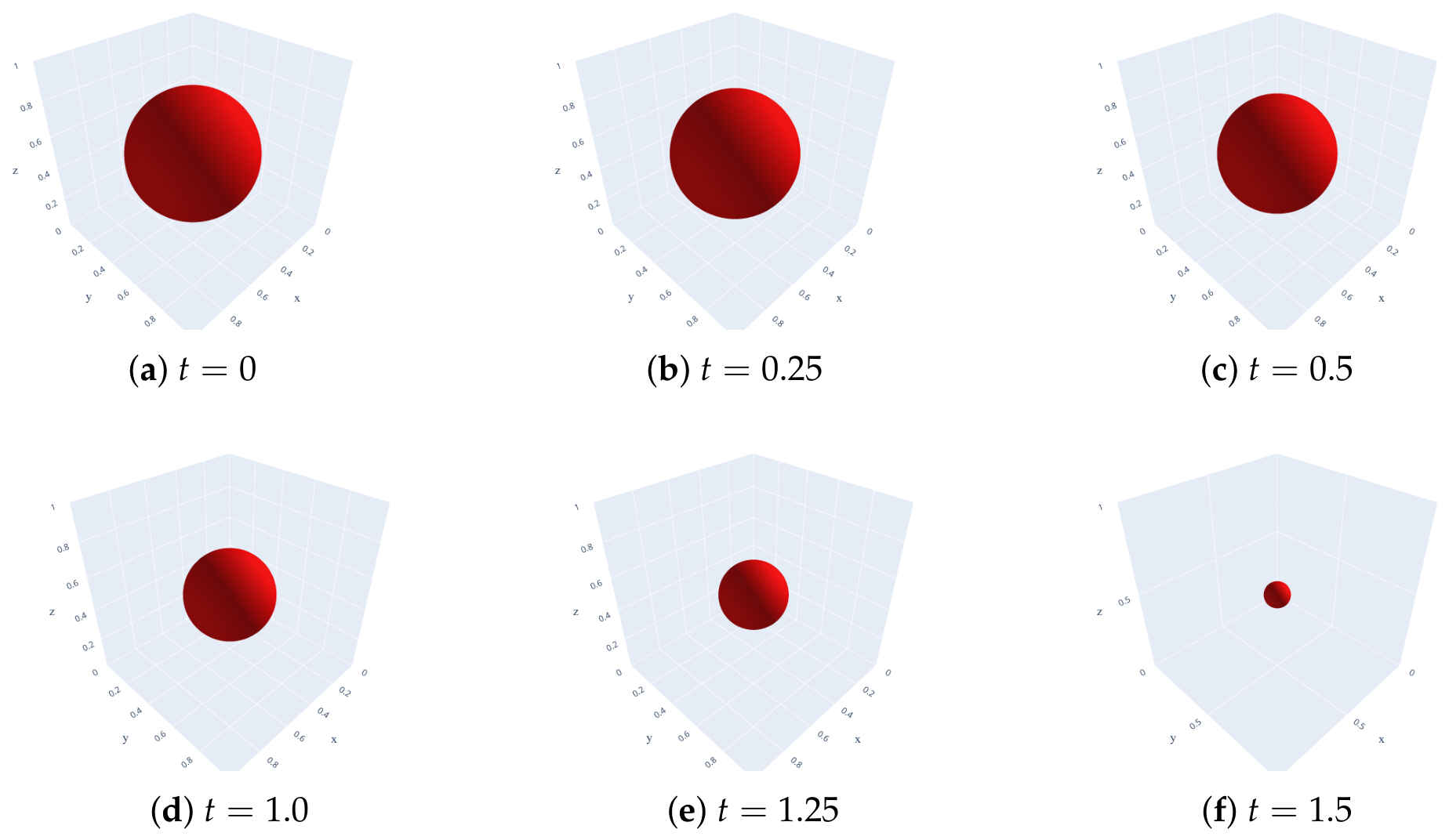
Figure 16 shows the zero isosurface ($u=0$) of the predicted solution at t = 0, 0.25, 0.5, 1.0, 1.25, 1.5. The spherical interface gradually shrank over time, in good agreement with the results reported in [31].

Figure 16. Section 4.6: Zero isosurfaces of the predicted solution at $t=0,0.25,0.5,1.0,1.25,1.5$.

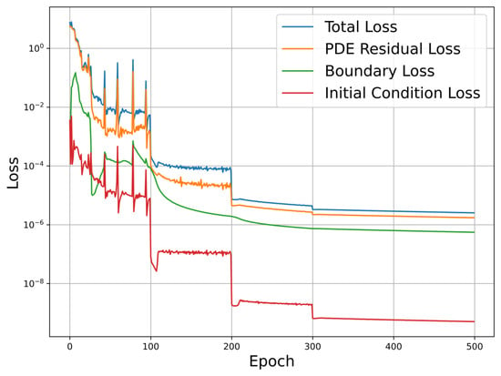
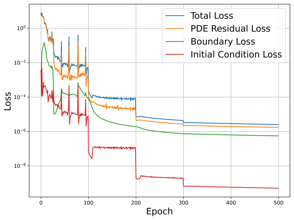
The training loss history is shown in Figure 17, which records the total loss together with the boundary, initial condition, and PDE residual losses. It can be observed that the total loss was predominantly contributed by the PDE residual. The rapid and stable decay of the loss demonstrates the convergence capability of the proposed STFE-PINN framework even for this three-dimensional problem.

Figure 17. Section 4.6: Training loss curve for the single-drop shrinking problem.

5. Conclusions

In this work, we proposed an enhanced physics-informed neural network framework, termed STFE-PINN, for solving the Allen–Cahn equation. The main contribution of this work is the introduction of two physically motivated feature embeddings: a spatial embedding based on a radial basis function network with learnable shape parameters, which improves the ability to capture sharp spatial transitions, and a temporal embedding that directly encodes the initial condition as an additional input feature, enabling the network to retain the initial state and accelerate convergence. For problems with long temporal horizons, a temporal domain decomposition strategy was further adopted to alleviate the difficulties of long-time optimization. Numerical experiments across one, two, and three dimensions, including comparisons with several existing improved PINN methods, consistently demonstrated that STFE-PINN achieved the optimal performance. This accuracy gain came with only a modest increase in the number of parameters compared with the standard PINN. Furthermore, the method exhibited rapid convergence and strong adherence to the underlying physical principles, including the energy dissipation law and the maximum bound principle.

Future work will extend the proposed framework to a broader class of time-dependent PDEs beyond the Allen–Cahn equation, including other phase field models, reaction-diffusion systems, and fluid dynamics problems. Additionally, we plan to investigate adaptive strategies for spatiotemporal sampling and to incorporate more general boundary conditions, further enhancing the versatility and efficiency of the method.

References

- Steinbach, I. Phase-field models in materials science. Model. Simul. Mater. Sci. Eng. 2009, 17, 073001. [Google Scholar] [CrossRef] [Scilit]
- Kim, J. Phase-field models for multi-component fluid flows. Commun. Comput. Phys. 2012, 12, 613–661. [Google Scholar] [CrossRef] [Scilit]
- Karma, A.; Kessler, D.A.; Levine, H. Phase-field model of mode III dynamic fracture. Phys. Rev. Lett. 2001, 87, 045501. [Google Scholar] [CrossRef] [Scilit] [PubMed]
- Bourdin, B.; Francfort, G.A.; Marigo, J.-J. Numerical experiments in revisited brittle fracture. J. Mech. Phys. Solids 2000, 48, 797–826. [Google Scholar] [CrossRef] [Scilit]
- Li, Y.; Kim, J. Multiphase image segmentation using a phase-field model. Comput. Math. Appl. 2011, 62, 737–745. [Google Scholar] [CrossRef] [Scilit]
- Shen, J.; Yang, X. Numerical approximations of Allen-Cahn and Cahn-Hilliard equations. Discret. Contin. Dyn. Syst. 2010, 28, 1669–1691. [Google Scholar] [CrossRef] [Scilit]
- Du, Q.; Nicolaides, R.A. Numerical analysis of a continuum model of phase transition. SIAM J. Numer. Anal. 1991, 28, 1310–1322. [Google Scholar] [CrossRef] [Scilit]
- Hussain, S.; Haq, F.; Shah, A.; Abduvalieva, D.; Shokri, A. Comparison of approximate analytical and numerical solutions of the Allen Cahn equation. Int. J. Differ. Equ. 2024, 2024, 8835138. [Google Scholar] [CrossRef] [Scilit]
- Lee, C.; Choi, Y.; Kim, J. An explicit stable finite difference method for the Allen-Cahn equation. Appl. Numer. Math. 2022, 182, 87–99. [Google Scholar] [CrossRef] [Scilit]
- Al-Bairaqdar, O.T.; Sabawi, Y.A.; Hasso, M.S. Efficient numerical solution of the Allen-Cahn equation via a non-lumping Galerkin finite element method. AIP Adv. 2025, 15, 075210. [Google Scholar] [CrossRef] [Scilit]
- Feng, X.; Li, Y. Analysis of symmetric interior penalty discontinuous Galerkin methods for the Allen-Cahn equation and the mean curvature flow. IMA J. Numer. Anal. 2015, 35, 1622–1651. [Google Scholar] [CrossRef] [Scilit]
- Lee, H.G.; Lee, J.-Y. A second order operator splitting method for Allen-Cahn type equations with nonlinear source terms. Phys. A 2015, 432, 24–34. [Google Scholar] [CrossRef] [Scilit]
- Wang, Y. A high-order numerical scheme for Allen-Cahn equation via Strang splitting and Fourier spectral method. Highlights Sci. Eng. Technol. 2025, 159, 393–403. [Google Scholar] [CrossRef] [Scilit]
- Raissi, M.; Perdikaris, P.; Karniadakis, G.E. Physics-informed neural networks: A deep learning framework for solving forward and inverse problems involving nonlinear partial differential equations. J. Comput. Phys. 2019, 378, 686–707. [Google Scholar] [CrossRef] [Scilit]
- Hu, Z.; Kawaguchi, K.; Zhang, Z.; Karniadakis, G.E. Tackling the curse of dimensionality in fractional and tempered fractional PDEs with physics-informed neural networks. Comput. Methods Appl. Mech. Eng. 2024, 432, 117448. [Google Scholar] [CrossRef] [Scilit]
- Hutzenthaler, M.; Jentzen, A.; Kruse, T.; Nguyen, T.A. A proof that rectified deep neural networks overcome the curse of dimensionality in the numerical approximation of semilinear heat equations. SN Partial Differ. Equ. Appl. 2020, 1, 10. [Google Scholar] [CrossRef] [Scilit]
- Sirignano, J.; Spiliopoulos, K. DGM: A deep learning algorithm for solving partial differential equations. J. Comput. Phys. 2018, 375, 1339–1364. [Google Scholar] [CrossRef] [Scilit]
- E, W.; Yu, B. The deep Ritz method: A deep learning-based numerical algorithm for solving variational problems. Commun. Math. Stat. 2018, 6, 1–12. [Google Scholar] [CrossRef] [Scilit]
- Zang, Y.; Bao, G.; Ye, X.; Zhou, H. Weak adversarial networks for high-dimensional partial differential equations. J. Comput. Phys. 2020, 411, 109409. [Google Scholar] [CrossRef] [Scilit]
- Jagtap, A.D.; Mao, Z.; Adams, N.; Karniadakis, G.E. Physics-informed neural networks for inverse problems in supersonic flows. J. Comput. Phys. 2022, 466, 111402. [Google Scholar] [CrossRef] [Scilit]
- Zhang, G.; Lin, J.; Zhai, Q.; Yang, H.; Chen, X.; Leong, I.T.; Zhu, F. A priori error estimation for physics-informed neural networks solving Allen–Cahn and Cahn–Hilliard equations. Commun. Nonlinear Sci. Numer. Simul. 2026, 162, 110077. [Google Scholar] [CrossRef] [Scilit]
- Wight, C.L.; Zhao, J. Solving Allen-Cahn and Cahn-Hilliard equations using the adaptive physics informed neural networks. Commun. Comput. Phys. 2020, 29, 930–954. [Google Scholar] [CrossRef] [Scilit]
- Geng, Y.; Teng, Y.; Wang, Z.; Ju, L. A deep learning method for the dynamics of classic and conservative Allen-Cahn equations based on fully-discrete operators. J. Comput. Phys. 2024, 496, 112589. [Google Scholar] [CrossRef] [Scilit]
- Meng, X.; Li, Z.; Zhang, D.; Karniadakis, G.E. PPINN: Parareal physics-informed neural network for time-dependent PDEs. Comput. Methods Appl. Mech. Eng. 2020, 370, 113250. [Google Scholar] [CrossRef] [Scilit]
- Jagtap, A.D.; Kharazmi, E.; Karniadakis, G.E. Conservative physics-informed neural networks on discrete domains for conservation laws: Applications to forward and inverse problems. Comput. Methods Appl. Mech. Eng. 2020, 365, 113028. [Google Scholar] [CrossRef] [Scilit]
- Anagnostopoulos, S.J.; Toscano, J.D.; Stergiopulos, N.; Karniadakis, G.E. Residual-based attention in physics-informed neural networks. Comput. Methods Appl. Mech. Eng. 2024, 421, 116805. [Google Scholar] [CrossRef] [Scilit]
- Roy, P.; Castonguay, S.T. Exact enforcement of temporal continuity in sequential physics-informed neural networks. Comput. Methods Appl. Mech. Eng. 2024, 430, 117197. [Google Scholar] [CrossRef] [Scilit]
- Huang, X.; Alkhalifah, T. Efficient physics-informed neural networks using hash encoding. J. Comput. Phys. 2024, 501, 112760. [Google Scholar] [CrossRef] [Scilit]
- Zhang, T.; Yan, R.; Zhang, S.; Yang, D.; Chen, A. Application of Fourier feature physics-information neural network in model of pipeline conveying fluid. Thin-Walled Struct. 2024, 198, 111693. [Google Scholar] [CrossRef] [Scilit]
- McClenny, L.D.; Braga-Neto, U.M. Self-adaptive physics-informed neural networks. J. Comput. Phys. 2023, 474, 111722. [Google Scholar] [CrossRef] [Scilit]
- Kütük, M.; Yücel, H. Energy dissipation preserving physics informed neural network for Allen-Cahn equations. J. Comput. Sci. 2025, 87, 102577. [Google Scholar] [CrossRef] [Scilit]
- Wang, Z.; Chen, M.; Chen, J. Solving multiscale elliptic problems by sparse radial basis function neural networks. J. Comput. Phys. 2023, 492, 112452. [Google Scholar] [CrossRef] [Scilit]
- Bhatia, G.S.; Arora, G. Radial basis function methods for solving partial differential equations—A review. Indian J. Sci. Technol. 2016, 9, 105079. [Google Scholar] [CrossRef] [Scilit]
- Han Veiga, M.; Nassajian Mojarrad, F.; Nassajian Mojarrad, F. Learning a robust shape parameter for RBF approximation. Appl. Math. Comput. 2026, 510, 129706. [Google Scholar] [CrossRef] [Scilit]
- Bai, J.; Liu, G.-R.; Gupta, A.; Alzubaidi, L.; Feng, X.-Q.; Gu, Y.T. Physics-informed radial basis network (PIRBN): A local approximating neural network for solving nonlinear partial differential equations. Comput. Methods Appl. Mech. Eng. 2023, 415, 116290. [Google Scholar] [CrossRef] [Scilit]
- Kingma, D.P.; Ba, J. Adam: A method for stochastic optimization. In Proceedings of the 3rd International Conference on Learning Representations (ICLR), San Diego, CA, USA, 7–9 May 2015. [Google Scholar]
- Lee, H.G.; Hwang, Y.; Nam, Y.; Kim, S.; Kim, J. Benchmark problems for physics-informed neural networks: The Allen-Cahn equation. AIMS Math. 2025, 10, 7319–7338. [Google Scholar] [CrossRef] [Scilit]
- Jagtap, A.D.; Karniadakis, G.E. Extended physics-informed neural networks (XPINNs): A generalized space-time domain decomposition based deep learning framework for nonlinear partial differential equations. Commun. Comput. Phys. 2020, 28, 2002–2041. [Google Scholar] [CrossRef] [Scilit]
- Mattey, R.; Ghosh, S. A novel sequential method to train physics informed neural networks for Allen Cahn and Cahn Hilliard equations. Comput. Methods Appl. Mech. Eng. 2022, 390, 114474. [Google Scholar] [CrossRef] [Scilit]
- Ham, S.; Kim, J. Stability analysis for a maximum principle preserving explicit scheme of the Allen-Cahn equation. Math. Comput. Simul. 2023, 207, 453–465. [Google Scholar] [CrossRef] [Scilit]
- Ham, S.; Kang, S.; Hwang, Y.; Lee, G.; Kwak, S.; Jyoti; Kim, J. A fourth-order finite difference method for the Allen-Cahn equation. J. Comput. Appl. Math. 2025, 453, 116159. [Google Scholar] [CrossRef] [Scilit]
Disclaimer/Publisher’s Note: The statements, opinions and data contained in all publications are solely those of the individual author(s) and contributor(s) and not of MDPI and/or the editor(s). MDPI and/or the editor(s) disclaim responsibility for any injury to people or property resulting from any ideas, methods, instructions or products referred to in the content. |
© 2026 by the authors. Licensee MDPI, Basel, Switzerland. This article is an open access article distributed under the terms and conditions of the Creative Commons Attribution (CC BY) license.