Constancy of Functions via a Complement to Ekeland Variational Principle

Abstract

This paper establishes new criteria for the constancy of real-valued functions defined on general Banach spaces and on exterior domains in ${\mathbb{R}}^n$. The main analytical tool is a complement to Ekeland’s variational principle, while several auxiliary lemmas based on convex analysis play a crucial role in extending the argument to the non-convex framework of exterior domains. The obtained results establish constancy criteria under suitable growth assumptions at infinity, both in general Banach spaces and in the Euclidean setting. A key aspect of the analysis is the distinction between the whole-space and exterior-domain frameworks, showing that stronger asymptotic assumptions are required in the latter case. To illustrate the applicability of the general framework, we present an application to differentiable functions satisfying suitable symmetry-type assumptions on their derivatives.

1. Introduction

Within the vast landscape of mathematical research, a specific area of interest concerns the characterization of conditions under which a function must necessarily be constant. Without any doubt we can say that the most renowned result in this direction is Liouville’s theorem, which states that any harmonic function in ${\mathbb{R}}^n$ that is bounded (either from above or from below) must be constant. This theorem, which originates in complex analysis and partial differential equations, establishes a rigidity principle that has numerous applications, particularly in potential theory and continuum mechanics; derived from the maximum principle for harmonic functions, it has inspired profound generalizations in the context of partial differential equations, differential geometry, and geometric analysis. These so-called Liouville-type results extend to more general settings, including subharmonic functions, solutions of certain elliptic differential equations, and functions satisfying specific growth conditions at infinity. In recent decades, many Liouville-type theorems have been developed, extending the characterization of constant functions to broader classes of differential equation solutions. For instance, in the case of nonlinear elliptic equations, it has been shown that under suitable growth conditions, positive solutions must be constant. In 2020, Wang and Ruan in [1] provided a proof of Liouville’s theorem for a class of generalized harmonic functions using the parabolic equation method. In the same year, Filippucci, Pucci and Souplet in [2] established a Liouville-type theorem for an elliptic equation with superquadratic growth in the gradient, using monotonicity properties for the spherical averages of sub- and super-harmonic functions, combined with a gradient bound obtained by a local Bernstein argument. In 2021, Jiang, Wang and Zhu in [3] obtained Liouville-type results for the minimal surface equation in half space ${\mathbb{R}}_{+}^n$ with constant Neumann boundary value or linear Dirichlet boundary value. In 2022, Chang, Hu and Zhang in [4] proved a Liouville-type theorem for positive weak solutions of equations involving the p-Laplacian operator. More recently, in 2023, Lin and Ou in [5] derived Liouville-type results for positive harmonic functions on the unit disk with nonlinear boundary conditions, relying on an integral identity and certain Sobolev inequalities on the sphere.

These are only a few examples of Liouville-type theorems for various classes of differential equations. Similar results have also been established in the setting of Riemannian manifolds. For instance, Chen and Qiu in [6] investigated V-harmonic heat flows from complete Riemannian manifolds with non-negative Bakry–Émery curvature, deriving gradient estimates for ancient solutions and establishing a Liouville-type theorem. Additional recent examples of Liouville-type results can be found in [7,8,9].

A characteristic feature of Liouville-type theorems is that they are typically established for functions defined on the entire space. It is well known, however, that a harmonic function bounded from below and defined on an exterior domain is not necessarily constant. For example, if $\parallel ·\parallel$ denotes the Euclidean norm and $n\ge 3$, the function ${\displaystyle \frac{1}{{\parallel \mathbf{x}\parallel }^{n-2}}}$ restricted to ${\mathbb{R}}^n\setminus \overline{B}(\mathbf{0},r)$ provides a simple example of a nonconstant harmonic function bounded from below. For $n=2$, an explicit example can be found in [10], where the following Liouville-type theorem for harmonic function on exterior domains is also presented:

Theorem 1. 

Let K be a non-empty compact convex subset of ${\mathbb{R}}^2$ and $f:{\mathbb{R}}^2\setminus K\to \mathbb{R}$ be a harmonic function bounded from below. Assume that

$$\underset{\parallel \mathbf{x}\parallel \to +\infty }{lim}{\displaystyle \frac{f\left(\mathbf{x}\right)}{\parallel \mathbf{x}\parallel }}=0.$$

Then f is constant if and only if the relation

$$\parallel \nabla f\parallel \parallel \nabla f_{x_1{x}_1}\parallel \le \parallel \nabla f_{x_1}{\parallel }^2$$

holds pointwise in ${\mathbb{R}}^2\setminus K$.

The results of the present paper are not Liouville-type theorems in the strict sense and should rather be viewed as abstract constancy criteria. More precisely, we derive conditions ensuring that a function must be constant whenever its gradient norm satisfies suitable convexity or quasi-convexity properties together with appropriate growth assumptions at infinity. Although the functions considered here are not assumed to solve a prescribed differential equation, these criteria can be applied whenever the solutions of a given equation are known to satisfy the required assumptions. In this sense, Theorems 3–5 provide a general framework that may lead to Liouville-type results beyond the classical setting of partial differential equations. The main tool employed is a complement to Ekeland’s variational principle, originally introduced in 1996 and recalled in the next section in a slightly modified form adapted to exterior domains.

In the Euclidean case, the transition from the whole-space setting to exterior domains deserves particular attention. In fact, the geometry of exterior domains allows the existence of nonconstant functions satisfying conditions that would force constancy in the whole-space setting. Consequently, the asymptotic assumption appearing in the whole-space results must be strengthened when working in exterior domains. This phenomenon motivates the development of the convexity lemmas established in Section 2, which play a crucial role in extending the whole-space arguments to the exterior-domain setting. Moreover, the necessity of this stronger asymptotic assumption is illustrated later in the paper through an explicit example.

Exterior domains play an important role in several areas of contemporary research. They naturally arise in the study of nonlinear elliptic problems, asymptotic properties of solutions to partial differential equations, and numerical methods for problems posed in unbounded media. Examples of recent contributions in these directions can be found in [11,12].

Since the present paper builds upon the abstract framework developed in [10,13], it is worth briefly explaining its relation to those earlier contributions. Theorem 1 is obtained as an application of a complement to Ekeland’s variational principle (Theorem 2 recalled in the next section). A crucial step in that approach consists of proving a geometric criterion ensuring that a subset of an exterior domain coincides with the whole domain whenever it satisfies suitable conditions, one of which is that its convex hull coincides with the whole ambient space. In the two-dimensional setting considered in [10], this criterion is provided by Proposition 2.1. In particular, Proposition 2.1 of [10] coincides with Proposition 3 of the present paper when the latter is restricted to the case $n=2$. The present paper extends this geometric result to arbitrary dimension. Rather than attempting to generalize the argument of [10], whose extension to higher dimensions appears far from straightforward, the present paper develops new geometric arguments in Lemmas 1 and 2. These lemmas are established by means of an inductive procedure specifically designed to treat the higher-dimensional setting. These lemmas make it possible to establish Proposition 3 for every $n\ge 2$. This extension allows us to treat exterior domains in arbitrary dimensions and, consequently, to derive the general constancy criteria established in the present work.

The following section gathers the preliminary material needed for our analysis, including a geometric lemma essential for handling the case of functions defined on exterior domains of ${\mathbb{R}}^n$. The final section presents the constancy results both in the general framework of real Banach spaces and in the specific case of ${\mathbb{R}}^n$.

2. Preliminaries

In what follows, let $(X,\parallel ·{\parallel }_X)$ be a real Banach space whose topological dual will be denoted by $(X^{\ast },\parallel ·{\parallel }_{X^{\ast }})$. For each $x\in X$ and $r>0$, define $B(x,r)=\{y\in X:\parallel x-y{\parallel }_X<r\}$, $\overline{B}(x,r)$ the closure of $B(x,r)$, while for each $x,y\in X$, let $S(x,y)=\{\lambda x+(1-\lambda )y:\lambda \in [0,1\left]\right\}$. When $X={\mathbb{R}}^n$ we will consider on it the Euclidean norm, denoted with $\parallel ·\parallel$, and we represent a generic vector by $\mathbf{x}=(x_1,\dots ,x_n)$. Moreover, if W is a subspace of ${\mathbb{R}}^n$ we denote the orthogonal projection by $p_W:{\mathbb{R}}^n\to W$. Finally, for $A\subseteq {\mathbb{R}}^n$, we denote $A^{\perp }:=\{\mathit{u}\in {\mathbb{R}}^n:{\langle \mathit{u},\mathit{v}\rangle }_n=0,\forall \mathit{v}\in A\}$ where ${\langle ·,·\rangle }_n$ is the inner product in ${\mathbb{R}}^n$. If ${\mathit{u}}_{\mathbf{1}},\dots ,{\mathit{u}}_{\mathit{m}}$ ($m\in \mathbb{N}$) are m vectors of ${\mathbb{R}}^n$, we denote their Gramian matrix by $G({\mathit{u}}_{\mathbf{1}},\dots ,{\mathit{u}}_{\mathit{m}})$, namely $G({\mathit{u}}_{\mathbf{1}},\dots ,{\mathit{u}}_{\mathit{m}})=\left[{\langle {\mathit{u}}_{\mathit{i}},{\mathit{u}}_{\mathit{j}}\rangle }_n\right]$. It is obviously a symmetric matrix, and it is well known that $\det G({\mathit{u}}_{\mathbf{1}},\dots ,{\mathit{u}}_{\mathit{m}})\ge 0$ and all its eigenvalues are non-negative.

In the literature on convex analysis, convex functions are usually defined only on convex domains. However, in some of the results presented in this paper, the functions are defined on non-convex sets. This motivates the introduction of a more general notion of convexity for functions defined on non-convex domains. Following [14], we adopt these definitions.

Definition 1. 

Let $(X,\parallel ·{\parallel }_X)$ be a real Banach space, $E\subseteq X$ and $f:E\to \mathbb{R}$ be a function.

(i) 

f is convex if, for each $k\in \mathbb{N}$, $x_1,\dots ,x_k\in E$, ${\lambda }_1,\dots ,{\lambda }_k\in [0,1]$, such that ${\lambda }_1+\cdots +{\lambda }_k=1$ and ${\lambda }_1{x}_1+\cdots +{\lambda }_k{x}_k\in E$, one has

$$f({\lambda }_1{x}_1+\cdots {\lambda }_k{x}_k)\le {\lambda }_{1}f\left(x_1\right)+\cdots +{\lambda }_{k}f\left(x_k\right);$$

(1)

(ii) 

f is interval convex if, for each $x_1,x_2\in E$ such that $S(x_1,x_2)\subseteq E$, the restriction of f to $S(x_1,x_2)$ is convex.

It is well known that, if E is convex, the usual notion of convex function is equivalent to property (1) with $k=2$. Moreover, since the convexity of E implies $S(x_1,x_2)\subseteq E$, the two previous definitions are equivalent. Finally, if E is convex a function $f:E\to \mathbb{R}$ is quasi-convex if, for each $\alpha \in \mathbb{R}$, the set $\{x\in E:f(x)\le \alpha \}$ is convex (see, e.g., [15]).

A well-known property of convex functions is that a convex function defined on the whole space and bounded from above must be constant. When $X={\mathbb{R}}^n$, it is not difficult to show that a similar property holds even if the function is defined on the complement of a compact, convex set.

Proposition 1. 

Let $n\ge 2$, $K\subseteq {\mathbb{R}}^n$ be a compact, convex bounded set and $f:{\mathbb{R}}^n\setminus K\to \mathbb{R}$ be an interval convex function, bounded from above. Then f is constant.

Proof. 

Suppose, by contradiction, that there exist $\mathbf{x},\mathbf{y}\in {\mathbb{R}}^n\setminus K$ such that $f\left(\mathbf{x}\right)>f\left(\mathbf{y}\right)$. It is possible to assume that $S(\mathbf{x},\mathbf{y})\subseteq {\mathbb{R}}^n\setminus K$; if not, since ${\mathbb{R}}^n\setminus K$ is polygonally connected, there exist ${\mathbf{z}}_1,\dots ,{\mathbf{z}}_k\in {\mathbb{R}}^n\setminus K$ such that ${\displaystyle {\displaystyle {\displaystyle \bigcup _{i=0}^k}}S({\mathbf{z}}_i,{\mathbf{z}}_{i+1})\subseteq {\mathbb{R}}^n\setminus K}$ (with ${\mathbf{z}}_0=\mathbf{x}$ and ${\mathbf{z}}_{k+1}=\mathbf{y}$) and $f\left(\mathbf{x}\right)>f\left(\mathbf{y}\right)$ implies that there exists $i\in \{0,1,\dots ,k\}$ such that $f\left({\mathbf{z}}_i\right)>f\left({\mathbf{z}}_{i+1}\right)$. Since $S(\mathbf{x},\mathbf{y})\cap K=\varnothing$, by the classical separation theorem, there exists a half-space H such that $S(\mathbf{x},\mathbf{y})\subseteq H$ and $H\cap K=\varnothing$. It is easy to see that at least one of the two half-lines $R_1=\{\alpha \mathbf{x}+(1-\alpha )\mathbf{y}:\alpha \ge 0\}$ and $R_2=\{\alpha \mathbf{y}+(1-\alpha )\mathbf{x}:\alpha \ge 0\}$ is contained in H.

• In the first case ($R_1\subseteq H$), for each $\lambda \in ]0,1[$, ${\displaystyle \overline{\mathbf{x}}=\frac{1}{\lambda }\mathbf{x}+\left(1-\frac{1}{\lambda }\right)\mathbf{y}\in R_1}$, and the convexity of f restricted to H implies that

$$f\left(\mathbf{x}\right)=f(\lambda \overline{\mathbf{x}}+(1-\lambda )\mathbf{y})\le \lambda f\left(\overline{\mathbf{x}}\right)+(1-\lambda )f\left(\mathbf{y}\right)$$

which gives

$$f\left(\overline{\mathbf{x}}\right)\ge f\left(\mathbf{y}\right)+{\displaystyle \frac{f\left(\mathbf{x}\right)-f\left(\mathbf{y}\right)}{\lambda }}.$$

Taking $\lambda$ close to zero, the previous inequality contradicts the assumption that f is bounded from above. In the case $R_2\subseteq H$, for each $\lambda \in ]0,1[$, ${\displaystyle \overline{\mathbf{x}}=\frac{1}{1-\lambda }\mathbf{x}-\left(\frac{\lambda }{1-\lambda }\right)\mathbf{y}\in R_2}$, and the convexity of f restricted to H implies that

$$f\left(\mathbf{x}\right)=f(\lambda \mathbf{y}+(1-\lambda )\overline{\mathbf{x}})\le \lambda f\left(\mathbf{y}\right)+(1-\lambda )f\left(\overline{\mathbf{x}}\right)$$

which gives

$$f\left(\overline{\mathbf{x}}\right)\ge f\left(\mathbf{y}\right)+{\displaystyle \frac{f\left(\mathbf{x}\right)-f\left(\mathbf{y}\right)}{1-\lambda }}.$$

As $\lambda$ approaches 1, the previous inequality contradicts the fact that f is bounded from above. □

In what follows, we recall Theorem 2.3 of [10], which will serve as the primary tool for deriving our criteria for constancy. This result, in the case $K=\varnothing$, appeared in [13] as a consequence of a more general complement to Ekeland’s variational principle.

Theorem 2. 

Let $(X,\parallel ·{\parallel }_X)$ be a real Banach space, K a closed and bounded subset of X, and $f:X\setminus K\to \mathbb{R}$ a lower semicontinuous and Gâteaux differentiable function, bounded from below. Assume that

$$\underset{{\parallel x\parallel }_X\to +\infty }{lim\; sup}{\displaystyle \frac{f\left(x\right)}{{\parallel x\parallel }_X}}<+\infty .$$

Then, for every ${\displaystyle ϵ>\underset{{\parallel x\parallel }_X\to +\infty }{lim\; sup}\frac{f\left(x\right)}{{\parallel x\parallel }_X}}$, one has

$$\overline{\mathrm{conv}}\left(\right\{x\in X\setminus K:\parallel f^{\prime }{\left(x\right)\parallel }_{X^{\ast }}\le ϵ\left\}\right)=X.$$

A consequence of the previous result in the case $K=\varnothing$ is the following.

Proposition 2. 

Let $(X,\parallel ·{\parallel }_X)$ be a real Banach space and $f:X\to \mathbb{R}$ a lower semicontinuous and Gâteaux differentiable function, bounded from below. Assume that the function $\parallel f^{\prime }{(·)\parallel }_{X^{\ast }}$ is quasi-convex and lower semicontinuous. Then, one has

$$\underset{x\in X}{sup}{\parallel f^{\prime }\left(x\right)\parallel }_{X^{\ast }}\le \underset{{\parallel x\parallel }_X\to +\infty }{lim\; sup}{\displaystyle \frac{f\left(x\right)}{{\parallel x\parallel }_X}}.$$

(2)

Proof. 

The conclusion holds trivially if ${\displaystyle \underset{{\parallel x\parallel }_X\to +\infty }{lim\; sup}\frac{f\left(x\right)}{{\parallel x\parallel }_X}=+\infty }$. On the other hand, if ${\displaystyle \underset{x\in X}{sup}{\parallel f^{\prime }\left(x\right)\parallel }_{X^{\ast }}=0}$, then f is constant on X, ${\displaystyle \underset{{\parallel x\parallel }_X\to +\infty }{lim\; sup}\frac{f\left(x\right)}{{\parallel x\parallel }_X}=0}$ and the claim is proved in this case as well. Suppose that ${\displaystyle \underset{{\parallel x\parallel }_X\to +\infty }{lim\; sup}\frac{f\left(x\right)}{{\parallel x\parallel }_X}<+\infty }$, ${\displaystyle \underset{x\in X}{sup}{\parallel f^{\prime }\left(x\right)\parallel }_{X^{\ast }}>0}$ and that (2) does not hold. Choose $ϵ>0$ such that

$$\underset{{\parallel x\parallel }_X\to +\infty }{lim\; sup}{\displaystyle \frac{f\left(x\right)}{{\parallel x\parallel }_X}}<ϵ<\underset{x\in X}{sup}{\parallel f^{\prime }\left(x\right)\parallel }_{X^{\ast }}.$$

(3)

In this case, Theorem 2 ensures that $\overline{\mathrm{conv}}\left(\left\{x\in X:\parallel f^{\prime }{\left(x\right)\parallel }_{X^{\ast }}\le ϵ\right\}\right)=X$. Moreover, the assumptions on the function $\parallel f^{\prime }{(·)\parallel }_{X^{\ast }}$ ensure that the set $\left\{x\in X:\parallel f^{\prime }{\left(x\right)\parallel }_{X^{\ast }}\le ϵ\right\}$ is closed and convex; hence we get $\left\{f^{\prime }\left(x\right):x\in X\right\}\subseteq B({\theta }_{X^{\ast }},ϵ)$, contradicting (3). □

When $X={\mathbb{R}}^n$ the previous proposition holds even if the function f is defined on an exterior domain. To prove this fact, we need some preliminary results. First, we point out the following remark.

Remark 1. 

If $K\subseteq {\mathbb{R}}^n$ and $A\subseteq {\mathbb{R}}^n\setminus K$, it is straightforward to verify that the two assumptions

${\left(i\right)}_n$

$\mathrm{conv}\left(\mathrm{A}\right)={\mathbb{R}}^{\mathrm{n}}$;

${\left(ii\right)}_n$

For each convex set $C\subseteq {\mathbb{R}}^n\setminus K$, the set $A\cap C$ is convex;

are respectively equivalent to

${\left(j\right)}_n$

Every (open) half-space of ${\mathbb{R}}^n$ intersects A;

${\left(jj\right)}_n$

For each $\mathbf{x},\mathbf{y}\in A$ such that $S(\mathbf{x},\mathbf{y})\cap K=\varnothing$, one has $S(\mathbf{x},\mathbf{y})\subseteq A$.

We are now ready to prove the following ray lemma in ${\mathbb{R}}^2$.

Lemma 1. 

Let $K\subseteq {\mathbb{R}}^2$ be a bounded set and $A\subseteq {\mathbb{R}}^2\setminus K$ such that

${\left(i\right)}_2$

$\mathrm{conv}\left(\mathrm{A}\right)={\mathbb{R}}^2$;

${\left(ii\right)}_2$

For each convex set $C\subseteq {\mathbb{R}}^2\setminus K$, the set $A\cap C$ is convex.

Then, every half-line in ${\mathbb{R}}^2$ contains an element of A.

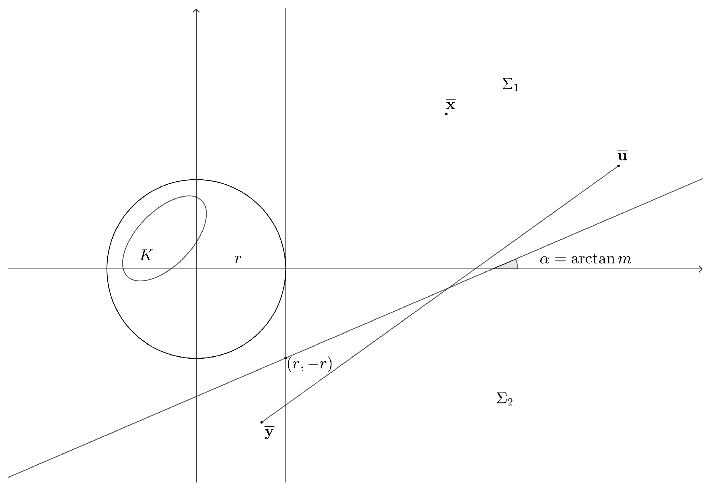
Proof. 

Fix a half-line in ${\mathbb{R}}^2$, and consider a Cartesian coordinate system on ${\mathbb{R}}^2$ such that the half-line coincides with the positive $x_1$-axis. Moreover, let $r>0$ such that $K\subseteq B(\mathbf{0},r)$. The claim is proved if we show that $\mathrm{\Sigma }\cap A\ne \varnothing$, where $\mathrm{\Sigma }=\left\{(x_1,0)\in {\mathbb{R}}^2:x_1>r\right\}$ (see Figure 1).

By ${\left(i\right)}_2$, there exists $\overline{\mathbf{x}}=({\overline{x}}_1,{\overline{x}}_2)\in \left\{(x_1,x_2)\in {\mathbb{R}}^2:x_1>r\right\}\cap A$. If ${\overline{x}}_2=0$, then $\mathbf{x}\in \mathrm{\Sigma }\cap A$ and the proof is complete. If ${\overline{x}}_2\ne 0$, assume that ${\overline{x}}_2>0$ (the case ${\overline{x}}_2<0$ is similar). Set ${\mathrm{\Sigma }}_1=\left\{(x_1,x_2)\in {\mathbb{R}}^2:x_1>r,x_2>0\right\}$, and ${\mathrm{\Sigma }}_2=\left\{(x_1,x_2)\in {\mathbb{R}}^2:x_1>r,x_2<0\right\}$. Clearly, $\mathbf{x}\in {\mathrm{\Sigma }}_1$. If there exists $\mathbf{z}\in {\mathrm{\Sigma }}_2\cap A$, then by ${\left(ii\right)}_2$, $S(\overline{\mathbf{x}},\mathbf{z})\subseteq A$ and the conclusion follows since $S(\overline{\mathbf{x}},\mathbf{z})\cap \mathrm{\Sigma }\ne \varnothing$. Hence, assume that ${\mathrm{\Sigma }}_2\cap A=\varnothing$. The set

$$\mathrm{\Gamma }:=\left\{{\displaystyle \frac{x_2+r}{x_1-r}}:(x_1,x_2)\in {\mathrm{\Sigma }}_1\cap A\right\}\subseteq ]0,+\infty [$$

(containing the slopes of all the lines passing through $(r,-r)$ and the points of ${\mathrm{\Sigma }}_1\cap A$) is non-empty since $({\overline{x}}_2+r)/({\overline{x}}_1-r)\in \mathrm{\Gamma }$. Let $m:=inf\mathrm{\Gamma }\in [0,+\infty [$ and define the half-plane ${\mathrm{\Sigma }}_3=\left\{(x_1,x_2)\in {\mathbb{R}}^2:x_2<m(x_1-r)-r\right\}$. By ${\left(i\right)}_2$, there exists $\overline{\mathbf{y}}=({\overline{y}}_1,{\overline{y}}_2)\in {\mathrm{\Sigma }}_3\cap A$. If $\overline{\mathbf{y}}\in \mathrm{\Sigma }$, the proof is complete. If $m>0$ and $\mathbf{y}\notin \mathrm{\Sigma }$, observe that $\mathbf{y}\notin {\mathrm{\Sigma }}_1$ either; indeed, if $\mathbf{y}\in {\mathrm{\Sigma }}_1$, then $m>({\overline{y}}_2+r)/({\overline{y}}_1-r)\in \mathrm{\Gamma }$, a contradiction. Since ${\mathrm{\Sigma }}_2\cap A=\varnothing$, it follows that $\overline{\mathbf{y}}\in \left\{(x_1,x_2)\in {\mathbb{R}}^2:x_1\le r,x_2<-r\right\}$. The same conclusion holds if $m=0$. Now, if ${\overline{y}}_1=r$ it is easy to observe that $S(\overline{\mathbf{x}},\overline{\mathbf{y}})$ avoids the set $\left\{(x_1,x_2)\in {\mathbb{R}}^2:x_1\le r,x_2\le -r\right\}$, where K is contained. Hence, by ${\left(jj\right)}_2$, $S(\overline{\mathbf{x}},\overline{\mathbf{y}})\subseteq A$. Since $S(\overline{\mathbf{x}},\overline{\mathbf{y}})\cap \mathrm{\Sigma }\ne \varnothing$, the claim follows. If ${\overline{y}}_1<r$, since $({\overline{y}}_2+r)/({\overline{y}}_1-r)>m$, there exists $\overline{\mathbf{u}}=({\overline{u}}_1,{\overline{u}}_2)\in {\mathrm{\Sigma }}_1\cap A$ such that $({\overline{y}}_2+r)/({\overline{y}}_1-r)>({\overline{u}}_1+r)/({\overline{u}}_1-r)$. This implies that $S(\overline{\mathbf{y}},\overline{\mathbf{u}})\cap K=\varnothing$ and thus $S(\overline{\mathbf{y}},\overline{\mathbf{u}})\subseteq A$. Again, the fact that $S(\overline{\mathbf{y}},\overline{\mathbf{u}})\cap \mathrm{\Sigma }\ne \varnothing$ yields the conclusion. □

Clearly, the previous lemma ensures that, under the same assumptions, every line in ${\mathbb{R}}^2$ contains infinite elements of A. We now wish to show that the same lemma holds for each dimension $n\in \mathbb{N}$, $n\ge 2$; it also holds for $n=1$ but this case will not be needed.

Lemma 2. 

Let $n\ge 2$, $K\subseteq {\mathbb{R}}^n$ be a bounded set and $A\subseteq {\mathbb{R}}^n\setminus K$ such that

${\left(i\right)}_n$

$\mathrm{conv}\left(\mathrm{A}\right)={\mathbb{R}}^{\mathrm{n}}$;

${\left(ii\right)}_n$

For each convex set $C\subseteq {\mathbb{R}}^n\setminus K$, the set $A\cap C$ is convex.

Then, every half-line in ${\mathbb{R}}^n$ contains an element of A.

Proof. 

We prove the statement by induction on n. By Lemma 1, the claim holds for $n=2$. Assume the result is true in n-dimensional spaces and let us prove it in dimension $n+1$. Let $K\subseteq {\mathbb{R}}^{n+1}$ be a bounded set and $A\subseteq {\mathbb{R}}^{n+1}\setminus K$ such that

${\left(i\right)}_{n+1}$

$\mathrm{conv}\left(\mathrm{A}\right)={\mathbb{R}}^{\mathrm{n}+1}$;

${\left(ii\right)}_{n+1}$

For each convex set $C\subseteq {\mathbb{R}}^{n+1}\setminus K$, the set $A\cap C$ is convex.

Fix a half-line in ${\mathbb{R}}^{n+1}$, and consider a Cartesian coordinate system on ${\mathbb{R}}^{n+1}$ such that this half-line coincides with the positive $x_1$-axis. Let $E={\mathbb{R}}^n\times \left\{0\right\}$. We now show that the sets $K_1=K\cap E$ (possibly empty) and $A_1=A\cap E$ satisfy assumptions ${\left(i\right)}_n$ and ${\left(ii\right)}_n$ so that we may apply the induction step. We will verify that assumption ${\left(j\right)}_n$ of Remark 1 and assumption ${\left(ii\right)}_n$ hold. To verify ${\left(j\right)}_n$, fix a generic half-space W of E, and denote its boundary by $W_0$, which is a hyperplane in E of dimension $n-1$. Then the set $W_0^{\perp }$ is the plane orthogonal to $W_0$ which contains the $x_{n+1}$-axis and has dimension 2. Let $K_2=p_{W_0^{\perp }}\left(K\right)$ and $A_2=p_{W_0^{\perp }}\left(A\right)\setminus p_{W_0^{\perp }}\left(K\right)$. We claim that $K_2$ and $A_2$ satisfy assumptions ${\left(j\right)}_2$ and ${\left(jj\right)}_2$ of Remark 1 in the plane $W_0^{\perp }$. To verify ${\left(j\right)}_2$, let L be a half-plane of $W_0^{\perp }$, with $L_0$ as boundary. Thanks to the boundedness of $K_2$, we can find another half-plane $M\subseteq L$ whose boundary is parallel to the line $L_0$ and such that $M\cap K_2=\varnothing$; this fact ensures that the set $T:=p_{W_0^{\perp }}^{-1}\left(M\right)$ is a half-space of ${\mathbb{R}}^{n+1}$ that does not intersect K. Thanks to condition ${\left(j\right)}_{n+1}$ of Remark 1, there exists $\mathbf{u}\in A\cap T$; in particular $p_{W_0^{\perp }}\left(\mathbf{u}\right)\in p_{W_0^{\perp }}\left(T\right)=M$ and then $p_{W_0^{\perp }}\left(\mathbf{u}\right)\notin K_2$. Therefore we have

$$p_{W_0^{\perp }}\left(\mathbf{u}\right)\in (p_{W_0^{\perp }}\left(A\right)\setminus p_{W_0^{\perp }}\left(K\right))\cap p_{W_0^{\perp }}\left(T\right)=A_2\cap M\subseteq A_2\cap L$$

which implies $A_2\cap L\ne \varnothing$. To verify ${\left(jj\right)}_2$, let us consider $\mathbf{v},\mathbf{w}\in A_2$, such that $S(\mathbf{v},\mathbf{w})\cap K_2=\varnothing$ and prove that $S(\mathbf{v},\mathbf{w})\subseteq A_2$. Since $\mathbf{v},\mathbf{w}\in A_2$, there exist ${\mathbf{v}}_{\mathbf{1}},{\mathbf{w}}_{\mathbf{1}}\in A$, such that $\mathbf{v}=p_{W_0^{\perp }}\left({\mathbf{v}}_{\mathbf{1}}\right)$, $\mathbf{w}=p_{W_0^{\perp }}\left({\mathbf{w}}_{\mathbf{1}}\right)$ and, clearly, ${\mathbf{v}}_{\mathbf{1}},{\mathbf{w}}_{\mathbf{1}}\notin K$. Trivially $S({\mathbf{v}}_{\mathbf{1}},{\mathbf{w}}_{\mathbf{1}})\cap K=\varnothing$; in fact, if there exists $\mathbf{z}\in S({\mathbf{v}}_{\mathbf{1}},{\mathbf{w}}_{\mathbf{1}})\cap K$, then $p_{W_0^{\perp }}\left(\mathbf{z}\right)\in S(\mathbf{v},\mathbf{w})\cap K_2$ which is a contradiction. Thanks to ${\left(jj\right)}_{n+1}$ of Remark 1, we get $S({\mathbf{v}}_{\mathbf{1}},{\mathbf{w}}_{\mathbf{1}})\subseteq A$ e then $S(\mathbf{v},\mathbf{w})\subseteq p_{W_0^{\perp }}\left(A\right)\setminus K_2=A_2$, as claimed. Hence, by Lemma 1 in the plane $W_0^{\perp }$, every line in that plane contains infinitely many points of $A_2$. In particular, if we consider the line $p_{W_0^{\perp }}\left(W\right)=W\cap W_0^{\perp }$, there exists $\mathbf{z}\in A_2\cap p_{W_0^{\perp }}\left(W\right)$, so there exists ${\mathbf{z}}_{\mathbf{1}}\in A\cap W$ with $p_{W_0^{\perp }}\left({\mathbf{z}}_{\mathbf{1}}\right)=\mathbf{z}$. Therefore ${\mathbf{z}}_{\mathbf{1}}\in A\cap W\subseteq A\cap E=A_1$, and so $A_1\cap W\ne \varnothing$, proving ${\left(j\right)}_n$ of Remark 1. To check assumption ${\left(ii\right)}_n$, fix a convex set $C\subseteq E\setminus K_1$, and prove that $A_1\cap C$ is convex. Clearly, we observe that $C\subseteq {\mathbb{R}}^{n+1}\setminus K$, so ${\left(ii\right)}_{n+1}$ ensures that $A\cap C$ is convex and then $A\cap C\cap E=A_1\cap C$ is convex, as claimed. Thus, by induction, every half-line of E contains an element of $A_1$. In particular the positive $x_1$-axis contains an element of $A_1$ that is also an element of A. Then the thesis is true in $n+1$-dimensional spaces as claimed. □

Clearly, the previous lemma assures that, under the same assumptions, every line in ${\mathbb{R}}^n$ contains infinite elements of A.

Proposition 3. 

Let $n\ge 2$, $K\subseteq {\mathbb{R}}^n$ be a compact, convex set and $A\subseteq {\mathbb{R}}^n\setminus K$ such that

(i) 

$\mathrm{conv}\left(\mathrm{A}\right)={\mathbb{R}}^{\mathrm{n}}$;

(ii) 

For each convex set $C\subseteq {\mathbb{R}}^n\setminus K$, the set $A\cap C$ is convex.

Then, $A={\mathbb{R}}^n\setminus K$.

Proof. 

Let us show that ${\mathbb{R}}^n\setminus K\subseteq A$. Fix ${\mathbf{u}}_{\mathbf{0}}\notin K$. By the hyperplane separation theorem, there exists a hyperplane $\mathrm{\Sigma }$ in ${\mathbb{R}}^n$ that strictly separates ${\mathbf{u}}_{\mathbf{0}}$ and K. Let ${\mathrm{\Sigma }}_1$ the hyperplane through ${\mathbf{u}}_{\mathbf{0}}$ parallel to $\mathrm{\Sigma }$, so ${\mathrm{\Sigma }}_1\cap K=\varnothing$. Consider a in ${\mathrm{\Sigma }}_1$ passing through ${\mathbf{u}}_{\mathbf{0}}$. By Lemma 2, there exist ${\mathbf{v}}_{\mathbf{1}},{\mathbf{v}}_{\mathbf{2}}\in A$ in the two half-lines of ${\mathrm{\Sigma }}_1$ having ${\mathbf{u}}_{\mathbf{0}}$ as the origin. Since ${\mathbf{u}}_{\mathbf{0}}\in S({\mathbf{v}}_{\mathbf{1}},{\mathbf{v}}_{\mathbf{2}})$ and, by $\left(ii\right)$, $S({\mathbf{v}}_{\mathbf{1}},{\mathbf{v}}_{\mathbf{2}})\subseteq A$, then ${\mathbf{u}}_{\mathbf{0}}\in A$ as claimed. □

Proposition 4. 

Let $n\ge 2$, $K\subseteq {\mathbb{R}}^n$ be a compact, convex set and $A\subseteq {\mathbb{R}}^n\setminus K$ such that

(i) 

$\mathrm{conv}\left(\mathrm{A}\right)={\mathbb{R}}^{\mathrm{n}}$;

(ii) 

For each open convex set $B\subseteq {\mathbb{R}}^n\setminus K$, the set $A\cap B$ is convex.

Then, $A={\mathbb{R}}^n\setminus K$.

Proof. 

We apply Proposition 3. Let $C\subseteq {\mathbb{R}}^n\setminus K$ be a convex set. We show that $A\cap C$ is convex. For ${\mathbf{u}}_{\mathbf{1}},{\mathbf{u}}_{\mathbf{2}}\in A\cap C$, we have $S({\mathbf{u}}_{\mathbf{1}},{\mathbf{u}}_{\mathbf{2}})\subseteq C\subseteq {\mathbb{R}}^n\setminus K$. Since $S({\mathbf{u}}_{\mathbf{1}},{\mathbf{u}}_{\mathbf{2}})$ is compact and convex and ${\mathbb{R}}^n\setminus K$ is open, there exists an open convex set B with $S({\mathbf{u}}_{\mathbf{1}},{\mathbf{u}}_{\mathbf{2}})\subseteq B\subseteq {\mathbb{R}}^n\setminus K$. By $\left(ii\right)$, $A\cap B$ is convex; hence $S({\mathbf{u}}_{\mathbf{1}},{\mathbf{u}}_{\mathbf{2}})\subseteq A\cap B$. Then $S({\mathbf{u}}_{\mathbf{1}},{\mathbf{u}}_{\mathbf{2}})\subseteq A\cap C$ and this proves the claim. □

The two propositions above are not true for $n=1$ as one can easily see taking $K=[0,1]$ and $A=]-\infty ,-1]\cup [2,+\infty [$. On the contrary, Lemma 2 also continues to hold for $n=1$ and it is very easy to prove it by contradiction.

Now, thanks to Proposition 4, we can prove that Proposition 2 holds even if the function f is defined on an exterior domain of ${\mathbb{R}}^n$.

Proposition 5. 

Let $n\ge 2$, $K\subseteq {\mathbb{R}}^n$ be a compact, convex set and $f:{\mathbb{R}}^n\setminus K\to \mathbb{R}$ be a differentiable function, bounded from below. Assume that, for each open convex set $B\subseteq {\mathbb{R}}^n\setminus K$, the restriction of the function $\parallel \nabla f(·)\parallel$ to B is quasi-convex and lower semicontinuous. Then, one has

$$\underset{\mathbf{x}\in {\mathbb{R}}^n\setminus K}{sup}\parallel \nabla f\left(\mathbf{x}\right)\parallel \le \underset{\parallel \mathbf{x}\parallel \to +\infty }{lim\; sup}{\displaystyle \frac{f\left(\mathbf{x}\right)}{\parallel \mathbf{x}\parallel }}.$$

Proof. 

Proceeding as in Proposition 2, choose $ϵ>0$ such that

$$\underset{\parallel \mathbf{x}\parallel \to +\infty }{lim\; sup}{\displaystyle \frac{f\left(\mathbf{x}\right)}{\parallel \mathbf{x}\parallel }}<ϵ<\underset{\mathbf{x}\in {\mathbb{R}}^n\setminus K}{sup}\parallel \nabla f\left(\mathbf{x}\right)\parallel .$$

(4)

Then $\overline{\mathrm{conv}}\left(\left\{\mathbf{x}\in {\mathbb{R}}^n\setminus K:\parallel \nabla f\left(\mathbf{x}\right)\parallel \le ϵ\right\}\right)={\mathbb{R}}^n$. Applying Proposition 4 to $A=\left\{\mathbf{x}\in {\mathbb{R}}^n\setminus K:\parallel \nabla f\left(\mathbf{x}\right)\parallel \le ϵ\right\}$, being in ${\mathbb{R}}^n$, clearly $\mathrm{conv}\left(\mathrm{A}\right)={\mathbb{R}}^{\mathrm{n}}$; moreover, if $B\subseteq {\mathbb{R}}^n\setminus K$ is an open convex set, we have that $A\cap B=\left\{\mathbf{x}\in B:\parallel \nabla f\left(\mathbf{x}\right)\parallel \le ϵ\right\}$ which is convex thanks to the assumptions on f. Applying Proposition 4, we see that $A={\mathbb{R}}^n\setminus K$, contradicting (4). Hence, the inequality follows. □

Remark 2. 

In the framework of Proposition 5, the quasi-convexity assumption is automatically satisfied whenever the function $\parallel \nabla f(·)\parallel$ is interval-convex in ${\mathbb{R}}^n\setminus K$. Indeed, if $B\subseteq {\mathbb{R}}^n\setminus K$ is an open convex set, obviously the restriction of the function $\parallel \nabla f(·)\parallel$ to B is convex and therefore quasi-convex. The same remark applies to Theorem 5.

3. Results

In this section, we establish the main results concerning the constancy of functions under the assumptions introduced above.

Theorem 3. 

Let $(X,\parallel ·{\parallel }_X)$ be a real Banach space and $f:X\to \mathbb{R}$ a lower semicontinuous and Gâteaux differentiable function that is bounded from below. Assume that the function $\parallel f^{\prime }{(·)\parallel }_{X^{\ast }}$ is quasi-convex and lower semicontinuous. Then the following two facts hold:

(i) 

If ${\displaystyle \underset{{\parallel x\parallel }_X\to +\infty }{lim\; sup}\frac{f\left(x\right)}{{\parallel x\parallel }_X}=0}$, then f is constant;

(ii) 

If there exists a strictly monotone function $g:[0,+\infty [\to \mathbb{R}$ such that the function $g(\parallel f^{\prime }(·){\parallel }_{X^{\ast }})$ is convex and

$$\underset{{\parallel x\parallel }_X\to +\infty }{lim\; sup}{\displaystyle \frac{f\left(x\right)}{{\parallel x\parallel }_X}}<+\infty$$

then $\parallel f^{\prime }{(·)\parallel }_{X^{\ast }}$ is constant.

Proof. 

To prove $\left(i\right)$, the constancy of f comes directly from Proposition 2 because we have

$$\underset{x\in X}{sup}{\parallel f^{\prime }\left(x\right)\parallel }_{X^{\ast }}\le \underset{{\parallel x\parallel }_X\to +\infty }{lim\; sup}{\displaystyle \frac{f\left(x\right)}{{\parallel x\parallel }_X}}=0.$$

To prove $\left(ii\right)$, let ${\displaystyle ϵ>\underset{{\parallel x\parallel }_X\to +\infty }{lim\; sup}\frac{f\left(x\right)}{{\parallel x\parallel }_X}}$. Theorem 2 assures that

$$\overline{\mathrm{conv}}\left(\right\{x\in X:\parallel f^{\prime }{\left(x\right)\parallel }_{X^{\ast }}\le ϵ\left\}\right)=X.$$

However, in our case, the set $\{x\in X:\parallel f^{\prime }\left(x\right){\parallel }_{X^{\ast }}\le ϵ\}$ is closed and convex, so the function $\parallel f^{\prime }{(·)\parallel }_{X^{\ast }}$ is bounded. Consequently, the convex function $g(\parallel f^{\prime }(·){\parallel }_{X^{\ast }})$ is bounded on X, and hence it is constant. The strict monotonicity of g implies that $\parallel f^{\prime }{(·)\parallel }_{X^{\ast }}$ is also constant. □

The following two facts are obtained by applying Theorem 3 to the particular cases $X=\mathbb{R}$ and $X={\mathbb{R}}^n$.

Example 1. 

Let $f:\mathbb{R}\to \mathbb{R}$ be a function bounded from below, with third derivative and satisfying

$$\underset{\left|x\right|\to +\infty }{lim\; sup}{\displaystyle \frac{f\left(x\right)}{\left|x\right|}}<+\infty .$$

If, for each $x\in \mathbb{R}$,

$$f^{\prime }\left(x\right)f^{‴}\left(x\right)\ge -{\left|f^{″}\left(x\right)\right|}^2$$

(5)

then f is constant.

Proof. 

It is easy to check that the second derivative of the function $|f^{\prime }{(·)|}^2$ is non-negative, thanks to inequality (5). Therefore, the function $|f^{\prime }{(·)|}^2$ is convex and then $|f^{\prime }(·)|$ is quasi-convex. Applying $\left(ii\right)$ of Proposition 3 with $g\left(t\right)=t^2$, for each $t\ge 0$, we observe that the function $|f^{\prime }(·)|$ is constant. Since $f^{\prime }$ is a continuous function, it must be constant. Thus, there exist $a,b\in \mathbb{R}$ such that $f\left(x\right)=ax+b$, for each $x\in \mathbb{R}$. The assumption that f is bounded from below forces $a=0$, and hence f is constant. □

Theorem 4. 

Let $f:{\mathbb{R}}^n\to \mathbb{R}$ be a differentiable function that is bounded from below and satisfies

$$\underset{\parallel \mathbf{x}\parallel \to +\infty }{lim\; sup}{\displaystyle \frac{f\left(\mathbf{x}\right)}{\parallel \mathbf{x}\parallel }}<+\infty .$$

Assume that the function $\parallel \nabla f(·)\parallel$ is quasi-convex and lower semicontinuous and that there exists a strictly monotone function $g:[0,+\infty [\to \mathbb{R}$ such that the function $g(\parallel \nabla f(·)\parallel )$ is convex. Then f is constant.

Proof. 

Thanks to Theorem 3, there exists $c\ge 0$ such that $\parallel \nabla f\left(\mathbf{x}\right)\parallel =c$, for each $\mathbf{x}\in {\mathbb{R}}^n$. It is well known that sufficiently regular global solutions of the Eikonal equation with a constant gradient norm are affine (see, for instance, [16] or [17]). However, the assumption that f is bounded from below forces the function to be constant. □

We now consider the case where the function f is defined on an exterior domain of ${\mathbb{R}}^n$. In this scenario, we cannot obtain a similar result as Theorem 4 because the solution of the Eikonal equation $\parallel \nabla f\parallel =c$ is not necessarily affine. For instance, if $r>0$ and $f:{\mathbb{R}}^n\setminus \overline{B}(\mathbf{0},r)$ is defined by $f\left(\mathbf{x}\right)=\parallel \mathbf{x}\parallel -r$, then f is a solution of the Eikonal equation $\parallel \nabla f\parallel =1$ but it is not affine. This example also explains why the growth assumption required in the exterior-domain setting is stronger than the corresponding assumption appearing in the whole-space case. Indeed, although $\parallel \nabla f\parallel =1$, one has

$$\underset{\parallel \mathbf{x}\parallel \to +\infty }{lim\; sup}{\displaystyle \frac{f\left(\mathbf{x}\right)}{\parallel \mathbf{x}\parallel }}=1,$$

so the weaker asymptotic condition used in the global framework is not sufficient to guarantee the constancy of f.

Theorem 5. 

Let $n\ge 2$, $K\subseteq {\mathbb{R}}^n$ be a compact, convex set and $f:{\mathbb{R}}^n\setminus K\to \mathbb{R}$ a differentiable function that is bounded from below. Assume that, for each open convex set $B\subseteq {\mathbb{R}}^n\setminus K$, the restriction of the function $\parallel \nabla f(·)\parallel$ to the set B is quasi-convex and lower semicontinuous. Then, the following two facts hold:

(i) 

If ${\displaystyle \underset{\parallel \mathbf{x}\parallel \to +\infty }{lim\; sup}\frac{f\left(\mathbf{x}\right)}{\parallel \mathbf{x}\parallel }=0}$, then f is constant;

(ii) 

If there exists a strictly monotone function $g:[0,+\infty [\to \mathbb{R}$ such that the function $g(\parallel \nabla f(·)\parallel )$ is interval convex and

$$\underset{\parallel \mathbf{x}\parallel \to +\infty }{lim\; sup}{\displaystyle \frac{f\left(\mathbf{x}\right)}{\parallel \mathbf{x}\parallel }}<+\infty$$

then $\parallel \nabla f(·)\parallel$ is constant.

Proof. 

As regards the proof of $\left(i\right)$, the constancy of f follows directly from Proposition 5 because we have

$$\underset{\mathbf{x}\in {\mathbb{R}}^n\setminus K}{sup}\parallel \nabla f\left(\mathbf{x}\right)\parallel \le \underset{\parallel \mathbf{x}\parallel \to +\infty }{lim\; sup}{\displaystyle \frac{f\left(\mathbf{x}\right)}{\parallel \mathbf{x}\parallel }}=0.$$

To prove $\left(ii\right)$, let ${\displaystyle ϵ>\underset{\parallel \mathbf{x}\parallel \to +\infty }{lim\; sup}\frac{f\left(\mathbf{x}\right)}{\parallel \mathbf{x}\parallel }}$. Theorem 2 assures that

$$\overline{\mathrm{conv}}\left(\right\{\mathbf{x}\in {\mathbb{R}}^n\setminus K:\parallel \nabla f\left(\mathbf{x}\right)\parallel \le ϵ\left\}\right)={\mathbb{R}}^n.$$

Applying Proposition 4 to the set $A=\{\mathbf{x}\in {\mathbb{R}}^n\setminus K:\parallel \nabla f\left(\mathbf{x}\right)\parallel \le ϵ\}$, it is clear that $\mathrm{conv}\left(\mathrm{A}\right)={\mathbb{R}}^{\mathrm{n}}$; moreover, if $B\subseteq {\mathbb{R}}^n\setminus K$ in an open convex set, we determine that $A\cap B=\left\{\mathbf{x}\in B:\parallel \nabla f\left(\mathbf{x}\right)\parallel \le ϵ\right\}$ which is convex thanks to the assumptions on f. Then $A={\mathbb{R}}^n\setminus K$; hence, the interval convex function $g(\parallel f^{\prime }(·)\parallel )$ is bounded from above on ${\mathbb{R}}^n\setminus K$ and thus, by Proposition 1, it is constant. The strict monotonicity of g implies that ${\parallel \nabla f(·)\parallel }_{X^{\ast }}$ is also constant. □

In the sequel, if $A\subseteq {\mathbb{R}}^n$ is an open set and $f:A\to \mathbb{R}$ is a function with partial derivatives, we denote for simplicity ${\displaystyle f_i=\frac{\partial f}{\partial x_i}}$, for each $i\in \{1,\dots ,n\}$.

Lemma 3. 

Let $n\ge 2$, $K\subseteq {\mathbb{R}}^n$ be a compact, convex set and $f\in C^2(R^n\setminus K)$ be a function with third partial derivatives and satisfying one of the following three assumptions:

(i) 

For each $i,j,k\in \{1,\dots ,n\}$ such that $i\ne j$ or $i\ne k$ or $j\ne k$, $f_{ijk}=0$. Additionally, for each $i\in \{1,\dots ,n\}$, $f_i{f}_{iii}\ge 0$.

(ii) 

There exists $u:{\mathbb{R}}^n\setminus K\to \mathbb{R}$, with $u\ge 0$, such that

$$u={\displaystyle {\displaystyle \sum _{k=1}^n}}{f}_k{f}_{kij}$$

for each $i,j\in \{1,\dots ,n\}$.

(iii) 

There exists $v:{\mathbb{R}}^n\setminus K\to \mathbb{R}$ such that, for each $i,j,k\in \{1,\dots ,n\}$, $v=f_{ijk}$, and ${\displaystyle {\displaystyle {\displaystyle \sum _{k=1}^n}}{f}_{k}v\ge 0}$.

Then the Hessian matrix of the function $F={\parallel \nabla f\parallel }^2$ is positive semidefinite in ${\mathbb{R}}^n\setminus K$.

Proof. 

Clearly, for each $i,j\in \{1,\dots ,n\}$, ${\displaystyle F_{ij}={\displaystyle {\displaystyle \sum _{k=1}^n}}(f_{ik}{f}_{jk}+f_k{f}_{kij})}$. Consequently, it is straightforward to verify that the Hessian matrix of F can be expressed as

$$G({\mathit{u}}_{\mathbf{1}},\dots ,{\mathit{u}}_{\mathit{n}})+\left[{\displaystyle {\displaystyle \sum _{k=1}^n}}{f}_k{f}_{kij}\right]$$

(6)

where ${\mathit{u}}_{\mathit{i}}=(f_{i1},\dots ,f_{in})$, pointwise in ${\mathbb{R}}^n\setminus K$. Now, we note that under assumption $\left(i\right)$, $\left(ii\right)$ or $\left(iii\right)$ every eigenvalue of the Hessian matrix of F is non-negative. We begin by observing that every eigenvalue of the matrix $G({\mathit{u}}_{\mathbf{1}},\dots ,{\mathit{u}}_{\mathit{n}})$ is non-negative. Under assumption $\left(i\right)$, ${\displaystyle \left[{\displaystyle {\displaystyle \sum _{k=1}^n}}{f}_k{f}_{kij}\right]}$ is a diagonal matrix, whose diagonal elements are $f_i{f}_{iii}$ and thus its eigenvalues are non negative. Therefore, Weyl’s monotonicity theorem (Corollary 4.3.12 of [18]) guarantees that each eigenvalue of matrix (6) is non-negative. Under assumption $\left(ii\right)$, ${\displaystyle \left[{\displaystyle {\displaystyle \sum _{k=1}^n}}{f}_k{f}_{kij}\right]}$ is a symmetric matrix, whose each element is equal to u, and hence the only non-zero eigenvalue is $nu$. Consequently, in this case, each eigenvalue of matrix (6) is also non-negative. Finally, if assumption $\left(iii\right)$ holds, then $\left(ii\right)$ is satisfied by choosing ${\displaystyle u={\displaystyle {\displaystyle \sum _{k=1}^n}}{f}_{k}v}$ and this completes the proof. □

Theorem 6. 

Let $n\ge 2$, $K\subseteq {\mathbb{R}}^n$ be a compact, convex set and $f\in C^2(R^n\setminus K)$ be a function that is bounded from below with third partial derivatives such that

(1) 

${\displaystyle \underset{\parallel \mathbf{x}\parallel \to +\infty }{lim\; sup}\frac{f\left(\mathbf{x}\right)}{\parallel \mathbf{x}\parallel }<+\infty }$ if $K=\varnothing$ or ${\displaystyle \underset{\parallel \mathbf{x}\parallel \to +\infty }{lim\; sup}\frac{f\left(\mathbf{x}\right)}{\parallel \mathbf{x}\parallel }=0}$ if $K\ne \varnothing$;

(2) 

Assumption $\left(i\right)$, $\left(ii\right)$ or $\left(iii\right)$ of Lemma 3 is satisfied.

Then f is constant.

Proof. 

In the case where $K=\varnothing$, the constancy of f follows directly from Theorem 4 with $g\left(t\right)=t^2$. In fact Lemma 3 ensures that the Hessian matrix of the function ${\parallel \nabla f\parallel }^2$ is positive semidefinite in ${\mathbb{R}}^n$. Therefore, both ${\parallel \nabla f\parallel }^2$ is convex and $\parallel \nabla f\parallel$ is quasi-convex. In the case where $K\ne \varnothing$, we apply the conclusion $\left(i\right)$ of Theorem 5. In this case, fixing an open convex set $B\subseteq {\mathbb{R}}^n\setminus K$, the Hessian matrix of the function ${\parallel \nabla f\parallel }^2$ is positive semidefinite in B. Therefore, the function ${\parallel \nabla f\parallel }^2$ is convex and $\parallel \nabla f\parallel$ is quasi-convex in B. □

Assumptions $\left(i\right)$, $\left(ii\right)$ and $\left(iii\right)$ of Lemma 3 are quite strong symmetry conditions on the derivatives of the function. While $\left(ii\right)$ is somewhat more general, $\left(i\right)$ and $\left(iii\right)$ identify the structure of the functions that satisfy them as explained in the following example.

Example 2. 

Let $n\ge 2$ and $K\subseteq {\mathbb{R}}^n$ be a compact, convex set and $K_i={\pi }_{E_i}\left(K\right)$ where $E_i$ is the $x_i$-axis. If, for each $i=1,\dots ,n$, $f_i:\mathbb{R}\setminus K_i\to \mathbb{R}$ and $g:\mathbb{R}\to \mathbb{R}$ are $n+1$ functions with third derivatives, and $P(x_1,\dots ,x_n)$ is a second-degree polynomial in the variables $x_1,\dots ,x_n$, then, the following applies:

(1) 

If, for each $i=1,\dots ,n$, $f_i^{\prime }{f}_i^{‴}\ge 0$, then the function $f:{\mathbb{R}}^n\setminus K\to \mathbb{R}$ defined by ${\displaystyle f\left(\mathbf{x}\right)={\displaystyle {\displaystyle \sum _{i=1}^n}}{f}_i\left(x_i\right)+P\left(\mathbf{x}\right)}$, for each $\mathbf{x}=(x_1,\dots ,x_n)\in {\mathbb{R}}^n\setminus K$, satisfies assumption $\left(i\right)$ of Lemma 3.

(2) 

If $g^{\prime }{g}^{‴}\ge 0$, then the function $f:{\mathbb{R}}^n\to \mathbb{R}$ defined by $f\left(\mathbf{x}\right)=g(x_1+\cdots +x_n)+P\left(\mathbf{x}\right)$, for each $\mathbf{x}=(x_1,\dots ,x_n)\in {\mathbb{R}}^n$, satisfies assumption (iii) of Lemma 3 with $v=g^{‴}$. Moreover, if ${\displaystyle \underset{\left|t\right|\to +\infty }{lim\; sup}\frac{g\left(t\right)}{\left|t\right|}<+\infty }$ and P is affine, then f satisfies assumption (1) of Theorem 6. This relies on the fact that

$$\underset{\parallel \mathbf{x}\parallel \to +\infty }{lim\; sup}{\displaystyle \frac{f\left(\mathbf{x}\right)}{\parallel \mathbf{x}\parallel }}\le \sqrt{n}\underset{\left|t\right|\to +\infty }{lim\; sup}{\displaystyle \frac{g\left(t\right)}{\left|t\right|}}+\underset{\parallel \mathbf{x}\parallel \to +\infty }{lim\; sup}{\displaystyle \frac{P\left(\mathbf{x}\right)}{\parallel \mathbf{x}\parallel }}.$$

Remark 3. 

It is worth emphasizing that assumptions $\left(i\right)$–$\left(iii\right)$ of Lemma 3 are not intended to characterize all situations in which the matrix (6) is positive semidefinite. Their role is rather to provide concrete sufficient conditions ensuring such a property. From this perspective, assumptions $\left(i\right)$–$\left(iii\right)$ should be regarded as one possible way to obtain the positive semidefiniteness of the matrix (6), a property that may also arise for other classes of functions.

Remark 4. 

Clearly, many nonconstant functions satisfying assumptions (2) of Theorem 6 and bounded from below fail the growth assumption (1), for instance, the functions $f:{\mathbb{R}}^n\setminus \overline{B}(\mathbf{0},r)$ (with $r>0$) defined by $f\left(\mathbf{x}\right)=\parallel \mathbf{x}\parallel -r$, for each $\mathbf{x}\in {\mathbb{R}}^n\setminus \overline{B}(\mathbf{0},r)$, and $g,h:{\mathbb{R}}^n\to \mathbb{R}$ defined by

$$g\left(\mathbf{x}\right)={\displaystyle {\displaystyle \sum _{i=1}^n}}{a}_i{e}^{x_i}$$

and

$$h\left(\mathbf{x}\right)={\displaystyle {\displaystyle \sum _{i=1}^n}}{a}_i{x}_i^{2m_i}$$

for each $\mathbf{x}=(x_1,\dots ,x_n)\in {\mathbb{R}}^n$, with $a_i\ge 0$ (at least one of them positive) and $m_i\in \mathbb{N}$.