Weak and Strong Gamma Distributed Delays in a Patch-Enabled SLBP Computer-Virus Model

Abstract

A patch-enabled delayed SLBP computer-virus model is extended by replacing the fixed delay in the breaking-out class with a distributed memory. Two gamma kernels are considered: the weak (single-stage) kernel, which encodes an exponentially fading memory, and the strong (two-stage) kernel, which encodes a memory peaked at a positive past time. The linear-chain trick converts the integro-differential equations into finite-dimensional ODE systems of dimension five and six, respectively, yielding polynomial characteristic equations amenable to a Routh–Hurwitz and Hopf analysis. We then carry out a direct numerical comparison of the three formulations on a common parameter set. The discrete-delay model loses stability through a Hopf bifurcation at a critical delay; both gamma models retain stability up to a substantially larger mean memory time, the weak kernel being the most stabilising and the strong kernel intermediate between the weak kernel and the discrete delay. The smearing of the past contribution by the gamma kernels therefore delays the onset of oscillations by a sizeable factor at fixed mean memory.

1. Introduction

Models of computer-virus and malware propagation exploit a structural analogy between malicious code spreading on a network and biological epidemics, originating with the contributions of Kermack and McKendrick [1] and Hethcote [2], and now firmly established in the modern cyber-security literature. The internal nodes of a network can be classified as susceptible, latent, breaking out, patched, quarantined, exposed, infected, or recovered, depending on the granularity of the model, in close analogy with classical SIR, SEIR, SEIQR, and SLBS frameworks. The susceptible–latent–breaking-out–patched (SLBP) family captures the typical life cycle of malicious code on hosts equipped with automatic patching procedures: a susceptible node becomes latently infected upon contact with an infectious source, transitions to a breaking-out state in which damage is actually produced, and may then receive a patch that restores immunity. Liu et al. [3] introduced a delayed patch-enabled SLBP model in which a single discrete delay encodes the time required by a breaking-out infection to feed back into the patching mechanism, and they used this delay as the bifurcation parameter.

The recent literature has explored a broad range of refinements of this baseline construction. Yu et al. [4] studied a delayed Susceptible–Latent–Breaking out–Patched–Susceptible (SLBPS) model in which the patch is granted a temporary immunity and derived the corresponding Hopf bifurcation together with an optimal control strategy. Wang et al. [5] extended the SEIQRS family to a two-delay impulse-controlled formulation, while Yang et al. [6] developed a fractional-order SVEIR-KS model and showed that the Hopf threshold depends on the fractional order in a non-trivial way. Yaagoub et al. [7] carried out the global analysis of a Caputo fractional-order infection model, and Ahmad et al. [8] obtained similar dynamics under an Atangana–Baleanu kernel. Zhou et al. [9] combined a fractional malware model with an optimal control formulation, and Bulavatsky and Bohaienko [10] introduced a piecewise-constant fractional order to capture stage-dependent memory.

The classical fixed-delay compartmental approach has been pursued in several directions. Cao et al. [11] added an age structure to the latent class, Bahashwan and Al-Tuwairqi [12] introduced heterogeneous immunity in the presence of removable storage devices, and Zhang and Li [13] examined a nonlinear countermeasure probability term. Zhu et al. [14] studied hybrid horizontal and vertical transmission. The dual-delay extension of Yang and Zhang [15] addressed industrial control networks, where the slower remediation and quarantine processes amplify the dynamical consequences of multiple lags. Behal et al. [16] systematically analysed a virus–patch model with a latent compartment.

A second line of work concerns wireless sensor networks and IoT systems, in which the limited resources of individual devices, the heterogeneous topology, and the presence of energy-saving sleep modes substantially modify the propagation dynamics. Martín-del Rey [17] proposed a compartmental WSN model with realistic monitoring regions, and Quiroga-Sánchez et al. [18] introduced the SEIRS-NIMFA framework for IoT malware propagation. B’ayir et al. [19] compared deterministic and stochastic representations on reduced scale-free topologies. The review by Nwokoye and Madhusudanan [20] provides a recent overview of these efforts. Stochastic perturbations have been studied by Nwokoye et al. [21], by Zhang et al. [22] for an e-SITR remote WSN model, and by Ayaz et al. [23] for a stochastic fractional formulation; Aleja et al. [24] introduced an awareness-coupled compartmental framework for cyber-epidemics, and Cui et al. [25] quantified the impact of insurance subsidies on the propagation of epidemic security risks. Other recent contributions focus on the impact of network topology and reaction-diffusion couplings [26], on numerical methods for fractional-order computer-virus models [27], and on optimal mitigation in IoT environments [28]. The general analysis of the discrete-delay characteristic equation in this family of models relies on the Hopf bifurcation framework recalled, for instance, in [29,30,31], while a complete proof of the basic reproduction number via the next-generation matrix approach is given in [32,33].

A fixed delay is mathematically convenient, but it assumes that every infected node experiences exactly the same waiting time. In computer-virus contexts this assumption is unrealistic: different machines have different hardware, operating systems, update schedules, and user behaviours, so the time spent before a breaking-out infection contributes to the delayed patch dynamics and is naturally distributed. The most common way to capture this heterogeneity is to replace the discrete delay with a memory average against a probability kernel. Among kernels, the gamma family has a privileged status because it is closed under the linear-chain trick: an integro-differential system with a gamma kernel can be rewritten as a finite-dimensional ODE system with auxiliary memory variables; we use the general formulation of Hurtado and Kirosingh [34]. This makes Routh–Hurwitz and Hopf analysis tractable, whereas the fixed-delay characteristic equation remains transcendental. Recent applications of the linear-chain trick to single-species logistic models [35], to memory effects in disease modelling with oscillatory time histories [36], to the stability of large ecosystems [37], and to multitrophic aquaculture systems [38] have shown that the shape of the kernel can either stabilise or destabilise the dynamics in ways that are not captured by a single scalar mean delay. In the stochastic context, the distributed-delay framework has been combined with white noise by Carletti [39] and, more recently, with delayed stochastic incubation by [40].

This paper carries out that extension for the SLBP model of [3]. The discrete delay in the breaking-out class is replaced first by a weak (single-stage) gamma memory and then by a strong (two-stage) gamma memory with the same mean. The two resulting ODE systems are five- and six-dimensional, respectively. The characteristic equations become polynomial, and one can compare directly the position of the Hopf bifurcation across the three formulations on a common parameter set.

The paper is organised as follows. Section 2 recalls the discrete-delay SLBP model. Section 3 introduces the distributed-delay extension and explains the linear-chain trick. Section 4 and Section 5 construct the equilibrium and the linearised system and prove the next-generation expression of the basic reproduction number. Section 6 writes the three characteristic equations in a unified form via the matrix determinant lemma. Section 7 states the Routh–Hurwitz and Hopf bifurcation tests with an explicit transversality formula. Section 8 reports the numerical comparison on a recalibrated parameter set, and Section 9 contains the discussion.

2. The Reference SLBP Model

The reference model partitions the internal nodes into susceptible $S\left(t\right)$, latent $L\left(t\right)$, breaking-out infected $B\left(t\right)$, and patched $P\left(t\right)$. The discrete-delay version studied in [3] reads

$$\begin{array}{c}{S}^{\prime }\left(t\right)=\lambda -({\beta }_{1}L\left(t\right)+{\beta }_{2}B\left(t\right))S\left(t\right)-\beta S\left(t\right)P\left(t\right)+c_{1}P\left(t\right)+c_{2}L\left(t\right)-\delta S\left(t\right),\hfill \\ L^{\prime }\left(t\right)=({\beta }_{1}L\left(t\right)+{\beta }_{2}B\left(t\right))S\left(t\right)-\beta L\left(t\right)P\left(t\right)-c_{2}L\left(t\right)-\alpha L\left(t\right)-\delta L\left(t\right),\hfill \\ B^{\prime }\left(t\right)=\alpha L\left(t\right)-\beta B(t-\tau )P\left(t\right)-\delta B\left(t\right),\hfill \\ P^{\prime }\left(t\right)=\beta (S\left(t\right)+L\left(t\right))P\left(t\right)-\beta B(t-\tau )P\left(t\right)-c_{1}P\left(t\right)-\delta P\left(t\right).\hfill \end{array}$$

Here $\lambda$ is the inflow of susceptible nodes, $\delta$ is the common removal rate, ${\beta }_1$ and ${\beta }_2$ are the infection rates due to latent and breaking-out nodes, $\alpha$ is the transition rate from latent to breaking-out infection, $c_2$ is the remediation rate of latent nodes, $c_1$ is the loss rate of patch protection, and $\beta$ controls the interaction with patched nodes. The only delay is the fixed value $\tau$ in the breaking-out variable, so the model concentrates the delayed feedback at one past time.

Remark 1.

The numerical experiments in [3] use a specific parameter set together with a reported endemic equilibrium $E^{\ast }$ and a reported Hopf threshold ${\tau }^{\ast }\simeq 35.65$. A direct substitution of those values into the printed steady-state equations does not give vanishing residuals, and an independent next-generation calculation gives a basic reproduction number below one for that parameter set, so the only positive equilibrium of the printed system is the disease-free one. More specifically, the parameter set printed in [3] is

$$\lambda =4,{\beta }_1=0.02,{\beta }_2=0.01,\beta =0.02,c_1=0.3,c_2=0.1,\delta =0.4,\alpha =0.1,$$

and the reported endemic equilibrium is $(19.6227,0.5138,1.9337,16.1464)$. Substitution of these values into the four steady-state equations gives the residual vector

$$(-5.8716,0.1069,-1.3465,-5.4243),$$

whose infinity norm is $5.8716$. Moreover, the next-generation expression derived below gives ${\mathcal{R}}_0=0.375<1$. Thus, the printed parameter/equilibrium pair is incompatible with the printed system, and the reported Hopf threshold cannot be reproduced from that pair. To keep the present analysis reproducible and to expose a genuine delay-induced Hopf bifurcation, we therefore work with a recalibrated set of infection rates while preserving all other parameters of [3]. This is the only deviation from the reference data, and the structure of the model is unchanged.

The transmission coefficients ${\beta }_1$, ${\beta }_2$, and $\beta$ are retained at the scale of the reference model and were recalibrated only to restore an epidemiologically meaningful endemic regime with ${\mathcal{R}}_0>1$ and a genuine delay-induced loss of stability. Their roles are distinct: ${\beta }_1$ and ${\beta }_2$ govern infection generated by latent and breaking-out nodes, respectively, whereas $\beta$ measures the interaction between infected and patched nodes. Thus, the selected values preserve the relative mechanisms of the original formulation while correcting the internal inconsistency described above. To assess local robustness, we repeated the spectral computation after separate $\pm 5\%$ perturbations of each transmission coefficient, keeping all remaining parameters fixed. This exercise is intended as a neighbourhood check around the recalibrated baseline, rather than as a global sensitivity analysis over the full parameter space. Whenever a Hopf threshold occurs in the explored interval, the qualitative ranking remains unchanged: the fixed-delay model destabilises first, followed by the multi-stage gamma memories, while the weak kernel has the largest threshold among the two baseline gamma cases. The perturbations shift the numerical threshold, as expected, but do not alter the principal conclusion that the shape of the memory distribution matters in addition to its mean.

3. Distributed-Delay Generalisation

To pass from the fixed delay to a distributed memory, the term $B(t-\tau )$ is replaced by the memory average

$$M\left(t\right)={\int }_0^{\infty }{K}_T\left(s\right)B(t-s)ds,$$

(1)

where $K_T\left(s\right)\ge 0$ and ${\int }_0^{\infty }{K}_T\left(s\right)ds=1$. The normalisation guarantees that $M\left(t\right)=B\left(t\right)$ whenever B is constant, so the gamma extensions share the constant equilibria of the non-delayed model. The distributed-delay SLBP system is then

$$\begin{array}{c}{S}^{\prime }\left(t\right)=\lambda -({\beta }_{1}L+{\beta }_{2}B)S-\beta SP+c_{1}P+c_{2}L-\delta S,\hfill \\ L^{\prime }\left(t\right)=({\beta }_{1}L+{\beta }_{2}B)S-\beta LP-c_{2}L-\alpha L-\delta L,\hfill \\ B^{\prime }\left(t\right)=\alpha L-\beta M\left(t\right)P-\delta B,\hfill \\ P^{\prime }\left(t\right)=\beta (S+L)P-\beta M\left(t\right)P-c_{1}P-\delta P,\hfill \end{array}$$

with $M\left(t\right)$ as in (1). The gamma family of kernels is special because it makes (1) equivalent to a finite-dimensional ODE through the linear-chain trick [34]. We use this construction twice.

3.1. Weak Gamma Memory

The single-stage gamma kernel is

$$K_w\left(s\right)={\displaystyle \frac{1}{T}}{e}^{-s/T},s\ge 0,$$

where $T>0$ is the mean memory time. A direct computation shows that ${\int }_0^{\infty }s{K}_w\left(s\right)ds=T$, so T is indeed the mean of the waiting-time distribution. If $Z\left(t\right)$ denotes the corresponding memory average,

$$Z\left(t\right)={\int }_0^{\infty }{K}_w\left(s\right)B(t-s)ds={\displaystyle \frac{1}{T}}{\int }_0^{\infty }{e}^{-s/T}B(t-s)ds,$$

the change of variable $u=t-s$ yields

$$Z\left(t\right)={\displaystyle \frac{1}{T}}{e}^{-t/T}{\int }_{-\infty }^t{e}^{u/T}B\left(u\right)du.$$

Differentiating with respect to t and applying Leibniz’s rule,

$$Z^{\prime }\left(t\right)=-{\displaystyle \frac{1}{T^2}}{e}^{-t/T}{\int }_{-\infty }^t{e}^{u/T}B\left(u\right)du+{\displaystyle \frac{1}{T}}B\left(t\right)={\displaystyle \frac{B\left(t\right)-Z\left(t\right)}{T}},$$

so the integro-differential system becomes a five-dimensional ODE,

$$\begin{array}{c}{S}^{\prime }=\lambda -({\beta }_{1}L+{\beta }_{2}B)S-\beta SP+c_{1}P+c_{2}L-\delta S,\hfill \\ L^{\prime }=({\beta }_{1}L+{\beta }_{2}B)S-\beta LP-c_{2}L-\alpha L-\delta L,\hfill \\ B^{\prime }=\alpha L-\beta ZP-\delta B,\hfill \\ P^{\prime }=\beta (S+L)P-\beta ZP-c_{1}P-\delta P,\hfill \\ Z^{\prime }=\frac{1}{T}(B-Z).\hfill \end{array}$$

The variable $Z\left(t\right)$ is interpreted as an exponentially weighted memory of the breaking-out nodes.

3.2. Strong Gamma Memory

The two-stage gamma kernel with the same mean T is

$$K_s\left(s\right)={\displaystyle \frac{4s}{T^2}}{e}^{-2s/T},s\ge 0.$$

A standard integration by parts gives ${\int }_0^{\infty }{K}_s\left(s\right)ds=1$ and ${\int }_0^{\infty }s{K}_s\left(s\right)ds=T$, so the kernel is normalised and has mean T. The mode is at $s=T/2$, in contrast with the weak kernel which is maximal at $s=0$. The kernel is therefore a better representation of a process whose delayed action requires two consecutive stages. Introducing two auxiliary memory variables $Z_1,Z_2$ via

$$Z_1\left(t\right)={\int }_0^{\infty }\frac{2}{T}{e}^{-2s/T}B(t-s)ds,Z_2\left(t\right)={\int }_0^{\infty }\frac{2}{T}{e}^{-2s/T}{Z}_1(t-s)ds,$$

a calculation analogous to the one above shows that the chain of two exponential integrals satisfies

$$Z_1^{\prime }=\frac{2}{T}(B-Z_1),Z_2^{\prime }=\frac{2}{T}(Z_1-Z_2),$$

and a Laplace-transform argument together with Fubini’s theorem confirms that $Z_2\left(t\right)={\int }_0^{\infty }{K}_s\left(s\right)B(t-s)ds$, i.e., $Z_2$ is the memory average against the strong gamma kernel. The strong distributed-delay model thus reads

$$\begin{array}{c}{S}^{\prime }=\lambda -({\beta }_{1}L+{\beta }_{2}B)S-\beta SP+c_{1}P+c_{2}L-\delta S,\hfill \\ L^{\prime }=({\beta }_{1}L+{\beta }_{2}B)S-\beta LP-c_{2}L-\alpha L-\delta L,\hfill \\ B^{\prime }=\alpha L-\beta Z_{2}P-\delta B,\hfill \\ P^{\prime }=\beta (S+L)P-\beta Z_{2}P-c_{1}P-\delta P,\hfill \\ Z_1^{\prime }=\frac{2}{T}(B-Z_1),\hfill \\ Z_2^{\prime }=\frac{2}{T}(Z_1-Z_2).\hfill \end{array}$$

The strong kernel suppresses contributions at $s=0$, which is the qualitative difference from the weak kernel. As we shall see, this changes the position of the Hopf threshold. The weak and strong gamma kernels are the first two members of the Erlang–gamma family with a prescribed mean T. They are the minimal cases that distinguish an exponentially decaying memory concentrated at the present from a genuinely staged, unimodal memory, while preserving a finite-dimensional ODE representation through the linear-chain construction. This makes it possible to derive characteristic polynomials and to apply Routh–Hurwitz criteria analytically. Higher-order Erlang kernels can be treated by the same chain construction, with n auxiliary stages and rate $n/T$; they are therefore used below as a numerical robustness check rather than developed as separate analytical models.

4. Equilibria and Basic Reproduction Number

Let $E^{\ast }=(S^{\ast },L^{\ast },B^{\ast },P^{\ast })$ denote a positive equilibrium of the non-delayed part of the model. Because the kernels are normalised, the memory variables at equilibrium satisfy $Z^{\ast }=B^{\ast }$ for the weak model and $Z_1^{\ast }=Z_2^{\ast }=B^{\ast }$ for the strong model. The equilibrium conditions reduce to

$$\lambda -({\beta }_1{L}^{\ast }+{\beta }_2{B}^{\ast })S^{\ast }-\beta S^{\ast }{P}^{\ast }+c_1{P}^{\ast }+c_2{L}^{\ast }-\delta S^{\ast }=0,$$

(2)

$$({\beta }_1{L}^{\ast }+{\beta }_2{B}^{\ast })S^{\ast }-\beta L^{\ast }{P}^{\ast }-(c_2+\alpha +\delta )L^{\ast }=0,$$

(3)

$$\alpha L^{\ast }-\beta B^{\ast }{P}^{\ast }-\delta B^{\ast }=0,$$

(4)

$$\beta (S^{\ast }+L^{\ast }-B^{\ast })P^{\ast }-(c_1+\delta )P^{\ast }=0.$$

(5)

Proposition 1.

At any positive endemic equilibrium with $P^{\ast }>0$, the following identities hold:

$$S^{\ast }+L^{\ast }-B^{\ast }={\displaystyle \frac{c_1+\delta }{\beta }},\lambda -\delta N^{\ast }-2\beta B^{\ast }{P}^{\ast }=0,$$

(6)

where $N^{\ast }=S^{\ast }+L^{\ast }+B^{\ast }+P^{\ast }$ is the total population at equilibrium.

Proof. 

Equation (5) factorises as $P^{\ast }\left[\beta (S^{\ast }+L^{\ast }-B^{\ast })-(c_1+\delta )\right]=0$. Since $P^{\ast }>0$, the bracket must vanish, giving the first identity. To obtain the second, sum Equations (2)–(5): the bilinear infection terms cancel pairwise, the remediation terms $c_2{L}^{\ast }$ and the patch-loss terms $c_1{P}^{\ast }$ cancel, and the delayed coupling terms contribute $-\beta B^{\ast }{P}^{\ast }$ to the equation for B and $-\beta B^{\ast }{P}^{\ast }$ to the equation for P. The remaining linear terms in $S^{\ast },L^{\ast },B^{\ast },P^{\ast }$ all carry the coefficient $-\delta$, so the sum becomes

$$\lambda -\delta (S^{\ast }+L^{\ast }+B^{\ast }+P^{\ast })-2\beta B^{\ast }{P}^{\ast }=0,$$

which is the second identity. □

The closed identity (6) prevents a fully algebraic closed form, but constrains the equilibrium to a one-parameter family that is straightforwardly solved numerically.

Setting $L=B=P=0$ in Equation (2) gives $S=\lambda /\delta$, so the disease-free equilibrium is

$$E_0=(S_0,0,0,0),S_0={\displaystyle \frac{\lambda }{\delta }}.$$

Following the standard next-generation approach [32,33], we identify the infected compartments as $(L,B)$. Linearising the right-hand side of the L and B equations at $E_0$ and decomposing into new infections F and transitions V,

$$F=\left(\begin{array}{cc}{\beta }_1{S}_0& {\beta }_2{S}_0\\ 0& 0\end{array}\right),V=\left(\begin{array}{cc}{c}_2+\alpha +\delta & 0\\ -\alpha & \delta \end{array}\right),$$

we have $\det V=\delta (c_2+\alpha +\delta )>0$, so V is invertible and

$$V^{-1}={\displaystyle \frac{1}{\delta (c_2+\alpha +\delta )}}\left(\begin{array}{cc}\delta & 0\\ \alpha & c_2+\alpha +\delta \end{array}\right).$$

A direct computation yields

$$F{V}^{-1}={\displaystyle \frac{S_0}{\delta (c_2+\alpha +\delta )}}\left(\begin{array}{cc}{\beta }_1\delta +{\beta }_2\alpha & {\beta }_2(c_2+\alpha +\delta )\\ 0& 0\end{array}\right).$$

The matrix $F{V}^{-1}$ has a single non-zero eigenvalue, equal to its trace, so the basic reproduction number is

$${\mathcal{R}}_0=\rho \left(F{V}^{-1}\right)={\displaystyle \frac{S_0\left({\beta }_1\delta +{\beta }_2\alpha \right)}{\delta (c_2+\alpha +\delta )}}.$$

(7)

The endemic equilibrium considered below satisfies ${\mathcal{R}}_0>1$, which is consistent with its positivity.

5. Linearisation

Write perturbations around $E^{\ast }$ as $x\left(t\right)={(s,\ell ,b,p)}^T$ for the four physical compartments. The linearisation takes the form

$$x^{\prime }\left(t\right)=Ax\left(t\right)+dm\left(t\right),$$

where $m\left(t\right)$ is the perturbation of the memory variable: $m\left(t\right)=b(t-\tau )$ for the fixed delay, $m\left(t\right)=z\left(t\right)$ for the weak gamma model, and $m\left(t\right)=z_2\left(t\right)$ for the strong gamma model. A direct computation of the Jacobian of the non-delayed coupling, together with the contributions $-\beta P^{\ast }m\left(t\right)$ and $-\beta P^{\ast }m\left(t\right)$ in the third and fourth equations, gives the matrices

$$A=\left(\begin{array}{cccc}{a}_{11}& a_{12}& a_{13}& a_{14}\\ a_{21}& a_{22}& a_{23}& a_{24}\\ 0& a_{32}& a_{33}& a_{34}\\ a_{41}& a_{42}& 0& a_{44}\end{array}\right),d=\left(\begin{array}{c}0\\ 0\\ -\beta P^{\ast }\\ -\beta P^{\ast }\end{array}\right),$$

with entries

$$\begin{array}{cc}{a}_{11}=-{\beta }_1{L}^{\ast }-{\beta }_2{B}^{\ast }-\beta P^{\ast }-\delta ,\hfill & a_{12}=c_2-{\beta }_1{S}^{\ast },\hfill \\ a_{13}=-{\beta }_2{S}^{\ast },\hfill & a_{14}=c_1-\beta S^{\ast },\hfill \\ a_{21}={\beta }_1{L}^{\ast }+{\beta }_2{B}^{\ast },\hfill & a_{22}={\beta }_1{S}^{\ast }-\beta P^{\ast }-c_2-\alpha -\delta ,\hfill \\ a_{23}={\beta }_2{S}^{\ast },\hfill & a_{24}=-\beta L^{\ast },\hfill \\ a_{32}=\alpha ,\hfill & a_{33}=-\delta ,\hfill \\ a_{34}=-\beta B^{\ast },\hfill & a_{41}=\beta P^{\ast },\hfill \\ a_{42}=\beta P^{\ast },\hfill & a_{44}=\beta (S^{\ast }+L^{\ast }-B^{\ast })-c_1-\delta .\hfill \end{array}$$

Two structural zeros deserve a comment. The first is $a_{43}=0$: the variable B enters the equation for P only through the delayed quantity $M\left(t\right)$, so its non-delayed contribution to the fourth row of A vanishes, and the entire dependence on B in $P^{\prime }$ is carried by the delayed vector d. The second is $a_{44}=0$: from Proposition 1 we have $S^{\ast }+L^{\ast }-B^{\ast }=(c_1+\delta )/\beta$ at any positive endemic equilibrium, so

$$a_{44}=\beta ·{\displaystyle \frac{c_1+\delta }{\beta }}-c_1-\delta =0.$$

Thus the bare matrix A has the special structure

$$A=\left(\begin{array}{cccc}{a}_{11}& a_{12}& a_{13}& a_{14}\\ a_{21}& a_{22}& a_{23}& a_{24}\\ 0& \alpha & -\delta & a_{34}\\ \beta P^{\ast }& \beta P^{\ast }& 0& 0\end{array}\right).$$

This explains why the eigenvalues of A alone need not have negative real parts: in the limit $\tau \to \infty$, when the delayed coupling is effectively decoupled, the system may already destabilise. A direct numerical evaluation at the parameter set of Section 8 returns a real eigenvalue of A close to $0.0235$, in agreement with the upper plateau of the spectral curves shown later.

6. Characteristic Equations

The three characteristic equations can be written compactly through the scalar transfer function from $b\left(t\right)$ to the memory perturbation. For the fixed delay this transfer function is $H_d\left(\lambda \right)=e^{-\lambda \tau }$; for the weak gamma model it is $H_w\left(\lambda \right)=1/(1+\lambda T)$; and for the strong gamma model it is $H_s\left(\lambda \right)=4/{(2+\lambda T)}^2$, as one verifies by taking the Laplace transform of the linear-chain equations and eliminating the auxiliary variables (the rational form of $H_w$ and $H_s$ is the central reason why the gamma kernels admit a finite-dimensional realisation, in contrast with the irrational $H_d$). With $e_3={(0,0,1,0)}^T$, the linearised system gives in all three cases

$$\left(\lambda I_{4}Ad{e}_3^{T}H\left(\lambda \right)\right)x=0,$$

where $H\left(\lambda \right)$ is the appropriate transfer function. A non-trivial x exists iff

$$\det \left(\lambda I_{4}Ad{e}_3^{T}H\left(\lambda \right)\right)=0.$$

The matrix determinant lemma states that for any invertible matrix M and any vectors $u,v$,

$$\det (M+u{v}^T)=\det \left(M\right)\left(1+v^T{M}^{-1}u\right).$$

Applying this lemma with $M=\lambda I_4-A$, $u=-d$ and $v^T=e_3^{T}H\left(\lambda \right)$,

$$\det \left(\lambda I_{4}Ad{e}_3^{T}H\left(\lambda \right)\right)=\det (\lambda I_4-A)-H\left(\lambda \right)e_3^T\mathrm{adj}(\lambda I_4-A)d,$$

where we used ${(\lambda I_4-A)}^{-1}=\mathrm{adj}(\lambda I_4-A)/\det (\lambda I_4-A)$. Substituting each of the three transfer functions yields the discrete-delay quasi-polynomial

$$\det (\lambda I_4-A)-e_3^T\mathrm{adj}(\lambda I_4-A)d{e}^{-\lambda \tau }=0,$$

(8)

the weak-gamma rational characteristic equation, equivalent after multiplying by $(1+\lambda T)$ to the polynomial

$$(1+\lambda T)\det (\lambda I_4-A)-e_3^T\mathrm{adj}(\lambda I_4-A)d=0,$$

(9)

and the strong-gamma rational equation, equivalent after multiplying by ${(2+\lambda T)}^2$ to

$${(2+\lambda T)}^2\det (\lambda I_4-A)-4e_3^T\mathrm{adj}(\lambda I_4-A)d=0.$$

(10)

Since $\det (\lambda I_4-A)$ is a polynomial of degree exactly 4 in $\lambda$ and $e_3^T\mathrm{adj}(\lambda I_4-A)d$ is a polynomial of degree at most 3, the left-hand side of (9) is a polynomial of degree 5 with leading coefficient T, and the left-hand side of (10) is a polynomial of degree 6 with leading coefficient $T^2$. To apply the Routh–Hurwitz criterion below in its standard monic form, we therefore define, for $T>0$, the weak-gamma characteristic polynomial

$$P_w(\lambda ;T)={\displaystyle \frac{(1+\lambda T)\det (\lambda I_4-A)-e_3^T\mathrm{adj}(\lambda I_4-A)d}{T}},$$

(11)

and the strong-gamma characteristic polynomial

$$P_s(\lambda ;T)={\displaystyle \frac{{(2+\lambda T)}^2\det (\lambda I_4-A)-4e_3^T\mathrm{adj}(\lambda I_4-A)d}{T^2}}.$$

(12)

By construction $P_w(·;T)$ is monic of degree 5 and $P_s(·;T)$ is monic of degree 6, and the zeros of $P_w$ and $P_s$ coincide with those of (9) and (10), respectively. By contrast, Equation (8) is transcendental and has infinitely many roots.

Remark 2.

The same conclusion can be reached by writing the full linearised system in companion form. For the weak case, the $5\times 5$ block matrix

$${\mathcal{M}}_w\left(T\right)=\left(\begin{array}{cc}A& d\\ e_3^T/T& -1/T\end{array}\right)$$

acts on $(x,z)$, and a Schur-complement expansion gives

$$T\det (\lambda I_5-{\mathcal{M}}_w\left(T\right))=(1+\lambda T)\det (\lambda I_4-A)-e_3^T\mathrm{adj}(\lambda I_4-A)d=T{P}_w(\lambda ;T),$$

so that $\det (\lambda I_5-{\mathcal{M}}_w\left(T\right))=P_w(\lambda ;T)$. For the strong case, the $6\times 6$ companion matrix

$${\mathcal{M}}_s\left(T\right)=\left(\begin{array}{ccc}A& 0_{4\times 1}& d\\ (2/T)e_3^T& -2/T& 0\\ 0_{1\times 4}& 2/T& -2/T\end{array}\right)$$

acts on $(x,z_1,z_2)$ and a Schur-complement expansion on the $4+2$ block decomposition yields

$$T^2\det (\lambda I_6-{\mathcal{M}}_s\left(T\right))={(2+\lambda T)}^2\det (\lambda I_4-A)-4e_3^T\mathrm{adj}(\lambda I_4-A)d=T^2{P}_s(\lambda ;T),$$

so that $\det (\lambda I_6-{\mathcal{M}}_s\left(T\right))=P_s(\lambda ;T)$. The two derivations are equivalent.

7. Routh–Hurwitz Tests and Hopf Bifurcation

For the weak model, the monic polynomial $P_w(·;T)$ defined in (11) expands as

$$P_w(\lambda ;T)={\lambda }^5+r_1{\lambda }^4+r_2{\lambda }^3+r_3{\lambda }^2+r_4\lambda +r_5=0,$$

(13)

and for the strong model the monic polynomial $P_s(·;T)$ defined in (12) expands as

$$P_s(\lambda ;T)={\lambda }^6+q_1{\lambda }^5+q_2{\lambda }^4+q_3{\lambda }^3+q_4{\lambda }^2+q_5\lambda +q_6=0.$$

(14)

The coefficients $r_i=r_i\left(T\right)$ and $q_j=q_j\left(T\right)$ are rational functions of T and polynomial in the entries of A and in the components of d; their explicit symbolic expressions are lengthy and are computed numerically in Section 8.

Lemma 1

(Routh–Hurwitz, fifth order). The polynomial (13) has all its roots in the open left half-plane if and only if

$${\Delta }_1=r_1>0,{\Delta }_2=\det \left(\begin{array}{cc}{r}_1& 1\\ r_3& r_2\end{array}\right)>0,{\Delta }_3=\det \left(\begin{array}{ccc}{r}_1& 1& 0\\ r_3& r_2& r_1\\ r_5& r_4& r_3\end{array}\right)>0,$$

$${\Delta }_4=\det \left(\begin{array}{cccc}{r}_1& 1& 0& 0\\ r_3& r_2& r_1& 1\\ r_5& r_4& r_3& r_2\\ 0& 0& r_5& r_4\end{array}\right)>0,{\Delta }_5=r_5{\Delta }_4>0.$$

Lemma 2

(Routh–Hurwitz, sixth order). The polynomial (14) has all its roots in the open left half-plane if and only if the six Hurwitz determinants ${\Delta }_1,\dots ,{\Delta }_6$ associated with $P_s$ are all strictly positive, where ${\Delta }_j$ is the leading $j\times j$ principal minor of the Hurwitz matrix

$$H_s=\left(\begin{array}{cccccc}{q}_1& 1& 0& 0& 0& 0\\ q_3& q_2& q_1& 1& 0& 0\\ q_5& q_4& q_3& q_2& q_1& 1\\ 0& q_6& q_5& q_4& q_3& q_2\\ 0& 0& 0& q_6& q_5& q_4\\ 0& 0& 0& 0& 0& q_6\end{array}\right).$$

A Hopf bifurcation occurs along the family $T\mapsto P_w(·;T)$, respectively $T\mapsto P_s(·;T)$, when a pair of complex conjugate roots crosses the imaginary axis transversally, while all other roots remain in the open left half-plane. The next two propositions make this condition explicit.

Proposition 2

(Existence of pure imaginary roots). Suppose that the polynomial $P_w(·;T)$ has a pair of pure imaginary roots $\lambda =\pm i{\omega }_0$ at some $T=T_0>0$, with ${\omega }_0>0$. Then $({\omega }_0,T_0)$ is a real solution of the system

$$\mathrm{Re}{P}_w(i{\omega }_0;T_0)=0,\mathrm{Im}{P}_w(i{\omega }_0;T_0)=0.$$

(15)

The analogous statement holds for $P_s$ with the obvious replacements.

Proof. 

A polynomial with real coefficients takes complex conjugate values at conjugate arguments, so $\overline{P_w\left(i\omega \right)}=P_w(-i\omega )$. If $P_w(i{\omega }_0;T_0)=0$, then $P_w(-i{\omega }_0;T_0)=0$, and conversely. The vanishing of $P_w(i{\omega }_0;T_0)$ is equivalent to the simultaneous vanishing of its real and imaginary parts, which is exactly (15). □

Proposition 3

(Transversality condition). Let $\lambda \left(T\right)$ be a $C^1$ branch of roots of $P_w(·;T)=0$ with $\lambda \left(T_0\right)=i{\omega }_0$ a simple root, and assume that ${\partial }_{\lambda }{P}_w(i{\omega }_0;T_0)\ne 0$. Then

$${\displaystyle \frac{d\lambda }{dT}}{|}_{T=T_0}=-{\displaystyle \frac{{\partial }_T{P}_w(i{\omega }_0;T_0)}{{\partial }_{\lambda }{P}_w(i{\omega }_0;T_0)}},$$

(16)

and the transversality condition reads

$$\mathrm{Re}{\left.{\displaystyle \frac{d\lambda }{dT}}\right|}_{T=T_0}=-\mathrm{Re}\left({\displaystyle \frac{{\partial }_T{P}_w(i{\omega }_0;T_0)}{{\partial }_{\lambda }{P}_w(i{\omega }_0;T_0)}}\right)\ne 0.$$

(17)

Proof. 

Differentiating the implicit equation $P_w(\lambda \left(T\right);T)=0$ with respect to T gives ${\partial }_{\lambda }{P}_w·{\lambda }^{\prime }\left(T\right)+{\partial }_T{P}_w=0$, whence (16). The simplicity of the root $i{\omega }_0$ is exactly the assumption ${\partial }_{\lambda }{P}_w(i{\omega }_0;T_0)\ne 0$, which guarantees that the implicit function theorem applies and that a smooth root branch through $i{\omega }_0$ exists. □

Theorem 1

(Hopf bifurcation, weak gamma model). Assume that the endemic equilibrium $E^{\ast }$ exists and that all roots of the weak gamma polynomial (13) have negative real parts for every $T\in (0,T_0)$. If, at $T=T_0$, the system (15) admits a real solution $({\omega }_0,T_0)$ with ${\omega }_0>0$ such that $i{\omega }_0$ is a simple root of $P_w(·;T_0)$ and all remaining roots have negative real parts, and if the transversality condition (17) holds, then the weak gamma model undergoes a Hopf bifurcation at $T=T_0$ and the endemic equilibrium becomes unstable for $T>T_0$ in a one-sided neighbourhood of $T_0$.

Proof. 

Write the weak gamma system as $X^{\prime }=F(X;T)$, with $X={(S,L,B,P,Z)}^T$. Since F is smooth for $T>0$ and the equilibrium satisfies $Z^{\ast }=B^{\ast }$, the endemic equilibrium $X^{\ast }={(S^{\ast },L^{\ast },B^{\ast },P^{\ast },B^{\ast })}^T$ is independent of T and defines a smooth equilibrium branch. The Jacobian at $X^{\ast }$ is the block matrix $M_w\left(T\right)$. By the Schur-complement computation carried out in Section 6, the characteristic polynomial of $M_w\left(T\right)$ is exactly $P_w(\lambda ;T)$. Hence, the spectral assumptions on $P_w$ are precisely the spectral assumptions on the linearisation of the weak gamma ODE system. At $T=T_0$, the hypotheses give a simple conjugate pair $\lambda =\pm i{\omega }_0$, ${\omega }_0>0$, and all remaining eigenvalues strictly in the open left half-plane. Since ${\partial }_{\lambda }{P}_w(i{\omega }_0;T_0)\ne 0$, the implicit function theorem gives a $C^1$ eigenvalue branch $\lambda \left(T\right)$ satisfying $P_w(\lambda \left(T\right);T)=0$ and

$${\lambda }^{\prime }\left(T_0\right)=-{\displaystyle \frac{{\partial }_T{P}_w(i{\omega }_0;T_0)}{{\partial }_{\lambda }{P}_w(i{\omega }_0;T_0)}}.$$

The transversality condition states that $\mathrm{Re}{\lambda }^{\prime }\left(T_0\right)\ne 0$. Because all roots are assumed to have negative real parts for $T<T_0$, the crossing must occur from the left half-plane to the right half-plane as T increases through $T_0$. Therefore the endemic equilibrium loses asymptotic stability at $T=T_0$. The classical Hopf bifurcation theorem then implies the existence of a local branch of small-amplitude periodic solutions bifurcating from $X^{\ast }$ at $T=T_0$. The criticality and stability of this branch depend on the first Lyapunov coefficient, which is not determined by the spectral hypotheses alone. □

Theorem 2

(Hopf bifurcation, strong gamma model). Assume that the endemic equilibrium $E^{\ast }$ exists and that all roots of the strong gamma polynomial (14) have negative real parts for every $T\in (0,T_0)$. If, at $T=T_0$, the analogue of system (15) for $P_s$ admits a real solution $({\omega }_0,T_0)$ with ${\omega }_0>0$ such that $i{\omega }_0$ is a simple root of $P_s(·;T_0)$, all remaining roots have negative real parts, and the transversality condition holds, then the strong gamma model undergoes a Hopf bifurcation at $T=T_0$ and the endemic equilibrium becomes unstable for $T>T_0$ in a one-sided neighbourhood of $T_0$.

Proof. 

Identical to the proof of Theorem 1 after replacing $P_w$ by $P_s$, ${\mathcal{M}}_w\left(T\right)$ by ${\mathcal{M}}_s\left(T\right)$, the dimension five by six, and Lemma 1 by Lemma 2. In particular, the determinant identity becomes

$$T^2\det \left(\lambda I_6-{\mathcal{M}}_s\left(T\right)\right)={(2+\lambda T)}^2\det (\lambda I_4-A)-4e_3^T\mathrm{adj}(\lambda I_4-A)d=T^2{P}_s(\lambda ;T),$$

so that $\det (\lambda I_6-{\mathcal{M}}_s\left(T\right))=P_s(\lambda ;T)$ since $T>0$. The argument forcing $\mathrm{Re}{\lambda }^{\prime }\left(T_0\right)>0$ from the stability of all roots on $(0,T_0)$ goes through verbatim, hence $E^{\ast }$ becomes unstable for $T>T_0$ in a one-sided neighbourhood of $T_0$. □

8. Numerical Comparison

We now compare the three formulations on a common parameter set. As discussed in Remark 1, the values used here are

$$\lambda =4,{\beta }_1=0.15,{\beta }_2=0.08,\beta =0.11,c_1=0.3,c_2=0.1,\delta =0.4,\alpha =0.1.$$

With $S_0=\lambda /\delta =10$, the basic reproduction number (7) is

$${\mathcal{R}}_0={\displaystyle \frac{10(0.15·0.4+0.08·0.1)}{0.4·0.6}}={\displaystyle \frac{10·0.068}{0.24}}={\displaystyle \frac{17}{6}}\approx 2.833>1.$$

A Newton iteration on the system (2)–(5), initialised from the linear identity (6), returns the positive endemic equilibrium used below

$$E^{\ast }\approx (6.166,0.226,0.029,3.523).$$

Although the reference study states that its SLBP model has a unique positive equilibrium, this assertion cannot be used without verification here because the reference parameter/equilibrium pair is inconsistent with the printed equations. For the recalibrated parameter set, we therefore performed an independent numerical uniqueness check. After eliminating $B^{\ast }$ from (4) and using the positive-equilibrium identity (6), the equilibrium conditions reduce to a scalar equation on the biologically admissible interval $0<P^{\ast }<\lambda /\delta$. A systematic bracketing search on this interval, followed by root refinement and substitution into the full equilibrium system, detected exactly one positive root. Thus, within the stated numerical procedure, the equilibrium reported above is the only positive steady state detected for the parameter set used in the numerical analysis. This is a parameter-specific numerical finding and is not claimed as a global uniqueness theorem for all admissible parameter values. A direct check shows that $S^{\ast }+L^{\ast }-B^{\ast }=6.363\approx (c_1+\delta )/\beta =0.7/0.11=6.\overline{36}$ and $\delta N^{\ast }+2\beta B^{\ast }{P}^{\ast }\approx 3.978+0.022=4.000=\lambda$, confirming the closed identity of Proposition 1. The Jacobian of Section 5 evaluated at $E^{\ast }$ has eigenvalues with strictly negative real parts at $\tau =0$, while the eigenvalues of the bare matrix A (which describes the $\tau \to \infty$ limit, where the delayed coupling decouples) include the real value $\approx 0.0235$. Hence, a destabilisation must occur for some intermediate value of the delay parameter. The location of this destabilisation is the object of the comparison below. For the gamma models, the spectral abscissa was evaluated from all eigenvalues of the corresponding finite-dimensional linearisation. We first used a uniform grid with step $\Delta T={10}^{-2}$ to bracket every sign change of the spectral abscissa and then refined each bracket by bisection until its width was below ${10}^{-8}$. The reported critical value is the midpoint of the final bracket. At the refined value, the residual of the characteristic polynomial evaluated at the critical eigenvalue was checked to be below ${10}^{-8}$ in modulus, and the remaining eigenvalues were verified to have strictly negative real parts. The discrete-delay threshold was obtained analogously from the real and imaginary parts of the quasi-polynomial, using the grid only to initialise the nonlinear solver. These checks ensure that the reported thresholds do not depend materially on the plotting resolution.

8.1. Spectral Comparison

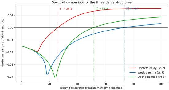
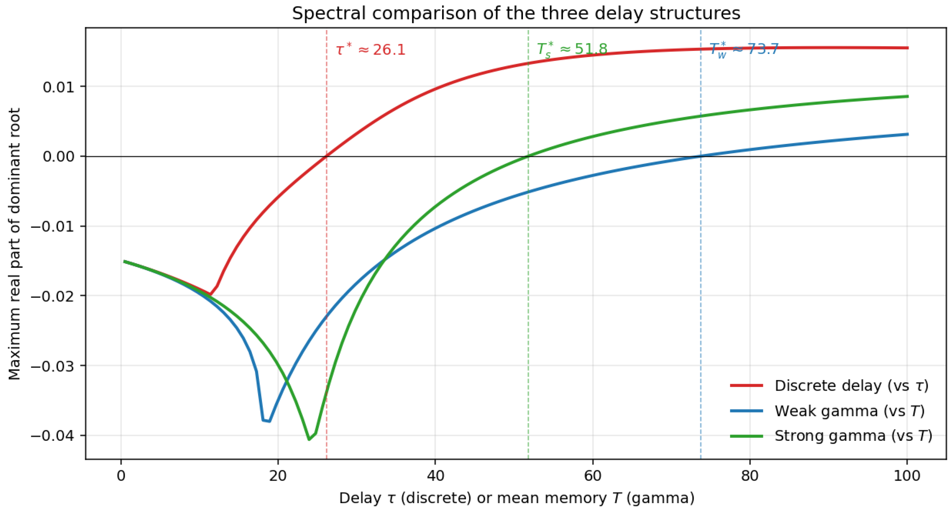
Figure 1 shows the maximum real part of the dominant characteristic root of each formulation as a function of the delay parameter ($\tau$ for the discrete model and the mean memory T for the gamma models). For the discrete Equation (8), the dominant root is tracked by Newton iteration on a fine grid; for the gamma models, the maximum real part is the leading eigenvalue of the five- or six-dimensional companion matrix associated with (9) or (10). The sign of this plotted quantity has a direct stability interpretation: negative values mean that perturbations of the endemic equilibrium decay, the zero level marks a Hopf threshold, and positive values indicate oscillatory growth in the linearised dynamics.

Three features are evident. First, the three curves agree at small delay, since all three transfer functions $H_d\left(\lambda \right)$, $H_w\left(\lambda \right)$, $H_s\left(\lambda \right)$ tend to one when $\tau ,T\to 0$. Second, the discrete-delay curve crosses the imaginary axis first, at

$${\tau }^{\ast }\approx 26.12,{\omega }^{\ast }\approx 0.077.$$

Third, the strong gamma curve crosses at $T_s^{\ast }\approx 51.80$ and the weak gamma curve at $T_w^{\ast }\approx 73.73$. Thus, at fixed mean memory, the smearing of the past contribution by the gamma kernels delays the onset of the bifurcation by a factor of roughly two for the strong kernel and roughly three for the weak kernel. The ordering of the thresholds is not a numerical accident: the discrete delay concentrates the whole feedback at one past instant, whereas the gamma kernels average the past contribution and reduce the effective phase shift responsible for the Hopf crossing.

Maximum real part of the dominant characteristic root as a function of the delay parameter ($\tau$ for the discrete model, T for the two gamma models). The three vertical dashed lines mark the Hopf thresholds. The discrete-delay model destabilises at ${\tau }^{\ast }\approx 26.1$, the strong gamma model at $T_s^{\ast }\approx 51.8$, and the weak gamma model at $T_w^{\ast }\approx 73.7$. For each gamma formulation, the critical conjugate pair was computed from the companion matrix and locally continued with respect to the mean memory time T. At the corresponding thresholds, the critical frequencies are

$${\omega }_w^{\ast }\approx 0.01910,{\omega }_s^{\ast }\approx 0.02765,$$

and

$$\mathrm{Re}{\left.{\displaystyle \frac{d{\lambda }_w}{dT}}\right|}_{T=T_w^{\ast }}\approx 1.6265\times {10}^{-4}>0,\mathrm{Re}{\left.{\displaystyle \frac{d{\lambda }_s}{dT}}\right|}_{T=T_s^{\ast }}\approx 4.1975\times {10}^{-4}>0.$$

Therefore, in both formulations, the critical pair is simple and crosses the imaginary axis transversally from left to right as T increases. This numerically verifies the transversality condition required by Theorems 1 and 2, or equivalently by Proposition 3.

As an additional robustness check, we also considered Erlang kernels with three and four stages, normalised to preserve the same mean memory time T. Their critical roots were tracked using the same spectral-abscissa grid, bisection refinement, and residual checks described above for the baseline gamma models. The associated critical thresholds are approximately $45.23$ and $41.79$, respectively. Thus, as the number of Erlang stages increases, the threshold approaches the fixed-delay value, consistent with the fact that higher-order Erlang distributions become increasingly concentrated around their mean. In particular, the ordering

$${\tau }^{\ast }<T_4^{\ast }<T_3^{\ast }<T_s^{\ast }<T_w^{\ast }$$

is preserved, showing that the distinction between weak and strong memory does not depend on considering only the two baseline gamma kernels.

The same picture is summarised quantitatively in

Table 1. Maximum real part of the dominant characteristic root of the three formulations as a function of the common delay parameter.

$\mathit{\tau }=\mathit{T}$	Discrete Delay	Weak Gamma	Strong Gamma
5	$-0.01677$	$-0.01686$	$-0.01681$
15	$-0.01249$	$-0.02508$	$-0.02318$
20	$-0.00583$	$-0.03489$	$-0.02996$
25	$-0.00100$	$-0.02467$	$-0.03861$
26.12	$\phantom{-}0.00000$	$-0.02297$	$-0.03383$
30	$+0.00326$	$-0.01817$	$-0.02162$
40	$+0.00964$	$-0.01033$	$-0.00720$
50	$+0.01293$	$-0.00576$	$-0.00079$

. Each row reports, for a fixed value of $\tau =T$, the maximum real part of the dominant root in the three formulations. The values show how the three models would lead to different operational conclusions for the same mean waiting time. For example, at $\tau =T=30$, the fixed-delay model is already unstable, while both gamma models remain stable. At $T=50$, the fixed-delay model is clearly beyond the Hopf threshold, but the strong gamma model is still just below it, and the weak gamma model is further from instability. These numbers therefore quantify the stabilising effect of memory dispersion, rather than only showing it graphically.

8.2. Time-Series Comparison

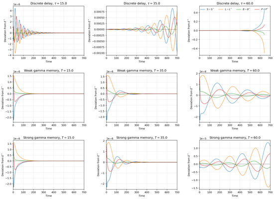
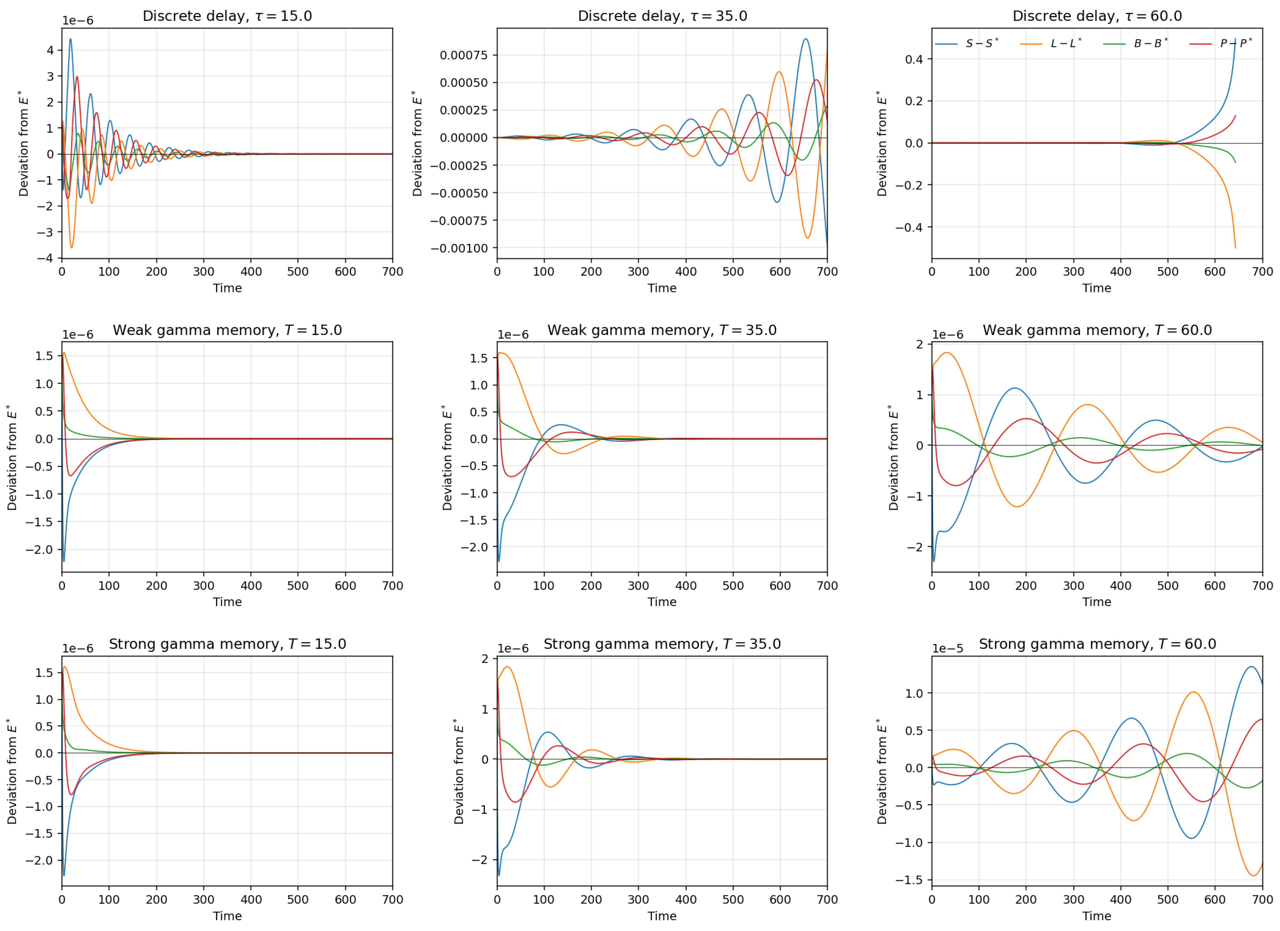
Figure 2 translates the spectral information into the time domain. Each panel reports the linear-regime response to a small perturbation of size ${10}^{-6}$ around $E^{\ast }$, displayed as deviations from the equilibrium. The three columns correspond to delay values $\tau =T\in \{15,35,60\}$, which sample the three relevant regimes. At $\tau =T=15$, well below every Hopf threshold, all three models damp the perturbation; nevertheless, the discrete model retains a more visible oscillatory transient because the fixed lag generates a stronger phase shift. At $\tau =T=35$, only the discrete model has lost stability, and its deviations grow with an oscillatory envelope, while both gamma models return to the equilibrium. At $\tau =T=60$, the discrete and strong-gamma models are unstable, whereas the weak-gamma model still damps the perturbation. The different vertical scales are intentional: they show that the same initial perturbation is amplified in the unstable panels but compressed rapidly in the stable gamma panels. The contrast at $T=60$ has a direct mechanistic interpretation. In the discrete-delay formulation, all feedback from breaking-out nodes is returned after the same waiting time. This perfectly synchronised feedback produces the largest phase lag and reinforces the oscillatory mode. The strong gamma kernel spreads the feedback over time, but its density is concentrated around the positive lag $T/2=30$; it therefore retains a substantial delayed component and is already beyond its Hopf threshold. In contrast, the weak kernel assigns its largest weight to the most recent past and exponentially downweights older breaking-out states. Its feedback is consequently less phase-shifted and responds more promptly to changes in the current infected population. This is why the weak gamma model remains stable at the common mean memory time $T=60$, whereas the discrete and strong-memory formulations do not.

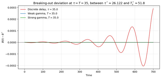
A direct comparison of the breaking-out class $B\left(t\right)$ between the three models at the same value $\tau =T=35$ is shown in Figure 3. This value lies between the fixed-delay threshold and the strong-gamma threshold. The contrast is therefore especially informative: the discrete model develops a clearly visible growing oscillation in the breaking-out population, whereas both gamma curves remain essentially flat at this scale because their perturbations are damped. In cyber-security terms, a deterministic feedback time of length 35 would predict sustained outbreaks, while a heterogeneous population of patching and activation times with the same mean still suppresses the perturbation.

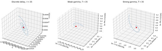
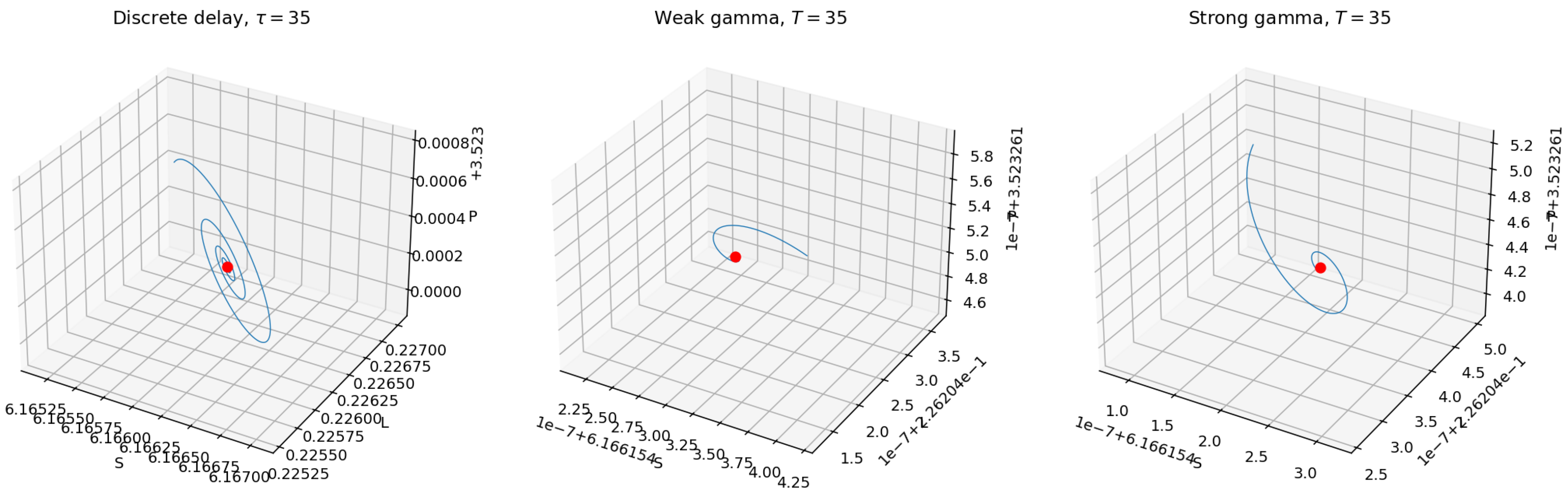
Finally, Figure 4 shows three-dimensional phase portraits in the $(S,L,P)$ subspace at $\tau =T=35$. The discrete model produces an outward spiral around $E^{\ast }$, signalling the unstable two-dimensional eigendirection generated by the Hopf pair. By contrast, the two gamma models give inward spirals that collapse onto $E^{\ast }$. The strong kernel converges more slowly than the weak kernel, consistent with the fact that its dominant real part is closer to zero in Table 1. The phase portraits therefore provide a geometric version of the same conclusion: distributed memory does not merely move the threshold numerically but changes the observable transient behaviour before instability is reached.

9. Discussion

The preceding analysis has established the common equilibrium structure, derived the characteristic equations, and located the stability boundaries numerically. We now interpret these results in terms of the timing profile of the delayed feedback and their implications for cyber-security modelling. The weak and strong gamma formulations are genuine extensions of the fixed-delay SLBP model. They preserve the biological and cyber-security interpretation of the original variables, but they replace the unrealistic assumption of a single waiting time with a distributed memory.

From the analytic side, the fixed delay contributes the factor $e^{-\lambda \tau }$, which has modulus one on the imaginary axis and can therefore produce strong phase shifts. By contrast, the weak gamma memory contributes $1/(1+\lambda T)$, and the strong gamma memory contributes $4/{(2+\lambda T)}^2$. Both these rational transfer functions damp out high-frequency components on the imaginary axis, with the weak kernel acting as a first-order low-pass filter and the strong kernel as a second-order one. The mechanism by which the gamma extensions delay the onset of oscillations is therefore the standard frequency-domain interpretation of memory smearing, and it is in qualitative agreement with the general results of Sawada et al. [35] and Mielke et al. [36] on distributed-delay logistic and SEIR-type systems.

From the numerical side, the comparison in Section 8 shows that on a common parameter set the discrete Hopf threshold ${\tau }^{\ast }\approx 26.12$ is followed by the strong gamma threshold $T_s^{\ast }\approx 51.80$ and then by the weak gamma threshold $T_w^{\ast }\approx 73.73$. The weak kernel, which concentrates probability mass near $s=0$, is the most stabilising of the three; the strong kernel, which is unimodal and concentrated around $s\simeq T/2$, lies in between. The ordering is consistent with the increasing concentration of the kernel mass at past times: the more the memory is spread over a long past interval, the smaller its phase-shift effect at any given frequency, and the larger the mean memory time that can be tolerated before destabilisation.

The take-home message is that the mean delay alone is not enough: the shape of the waiting-time distribution matters quantitatively for the Hopf threshold and qualitatively for the dynamics just past it. This has practical consequences for parameter estimation in cyber-security applications, where the waiting times before a breaking-out infection feeds back into the patching mechanism are heterogeneous and naturally distributed.

10. Conclusions

This paper has shown that replacing a fixed feedback delay by a distributed memory changes both the mathematical structure and the dynamical predictions of a patch-enabled SLBP computer-virus model. Because the weak and strong gamma kernels are normalised, the endemic equilibrium is the same as in the corresponding non-delayed formulation; the difference lies entirely in the way past breaking-out infections enter the feedback term. Through the linear-chain trick, the weak kernel gives a five-dimensional ODE system, and the strong kernel gives a six-dimensional ODE system. The resulting characteristic equations are polynomials, so the stability analysis can be carried out by finite-dimensional Routh–Hurwitz conditions and by an explicit Hopf transversality test.

The numerical comparison gives a clear message. For the recalibrated parameter set used here, the fixed-delay model loses stability at ${\tau }^{\ast }\approx 26.12$, whereas the strong and weak gamma models remain stable up to $T_s^{\ast }\approx 51.80$ and $T_w^{\ast }\approx 73.73$, respectively. Thus, two models with the same mean memory time can make different stability predictions if the shape of the waiting-time distribution is different. The fixed delay is the least stable formulation because it concentrates the whole feedback at one past instant. The strong gamma kernel is intermediate, while the weak gamma kernel is the most stabilising in the present parameter regime. The spectral plots, time-series simulations, breaking-out comparison, and phase portraits all support the same conclusion: memory dispersion delays the Hopf transition and suppresses oscillatory outbreak growth over a substantial range of mean waiting times.

From a modelling perspective, this means that the mean delay should not be used as the only descriptor of patching or malware-activation times. In realistic networks, devices differ in hardware, operating system, update schedule, user behaviour, and security policy; these differences produce a distribution of feedback times rather than a single deterministic lag. Using a fixed delay may therefore overestimate the tendency of the system to oscillate, especially when the real feedback is strongly dispersed.

Several extensions are natural. First, one can estimate the memory kernel from real patching, remediation, or malware-detection data and test whether empirical waiting-time distributions are closer to a weak gamma, a strong gamma, or a higher-order gamma law. Second, one can add stochastic perturbations to the gamma-memory systems, extending the white-noise setting of [3,23,39]. Third, one can combine distributed memory with network topology or spatial diffusion, in the spirit of [18,26], to quantify how heterogeneous connectivity interacts with heterogeneous feedback times.

References

- Kermack, W.O.; McKendrick, A.G. A contribution to the mathematical theory of epidemics. Proc. R. Soc. A 1927, 115, 700–721. [Google Scholar] [CrossRef] [Scilit]
- Hethcote, H.W. The mathematics of infectious diseases. SIAM Rev. 2000, 42, 599–653. [Google Scholar] [CrossRef] [Scilit]
- Liu, Z.; Madhusudanan, V.; Srinivas, M.N.; Nwokoye, C.H.; Geleto, T.D.; Gupta, P. An epidemic patch-enabled delayed model for virus propagation: Towards evaluating bifurcation and white noise. Math. Probl. Eng. 2022, 2022, 3763858. [Google Scholar] [CrossRef] [Scilit]
- Yu, X.; Zeb, A.; Liu, G. Hopf bifurcation and optimal control of a delayed SLBPS virus-patch model. Results Phys. 2022, 39, 105743. [Google Scholar] [CrossRef] [Scilit]
- Wang, J.; Chang, X.; Zhong, L. A SEIQRS computer virus propagation model and impulse control with two delays. Math. Methods Appl. Sci. 2025, 48, 6851–6865. [Google Scholar] [CrossRef] [Scilit]
- Yang, L.; Song, Q.; Liu, Y. Dynamics analysis of a new fractional-order SVEIR-KS model for computer virus propagation: Stability and Hopf bifurcation. Neurocomputing 2024, 598, 128075. [Google Scholar]
- Yaagoub, Z.; El Bhih, A.; Allali, K. Global analysis of a fractional-order infection model for the propagation of computer viruses. Model. Earth Syst. Environ. 2025, 11, 68. [Google Scholar] [CrossRef] [Scilit]
- Ahmad, I.; Bakar, A.A.; Ahmad, H.; Khan, A.; Abdeljawad, T. Investigating virus spread analysis in computer networks with Atangana–Baleanu fractional derivative models. Fractals 2024, 32, 2440043. [Google Scholar] [CrossRef] [Scilit]
- Zhou, Y.; Liu, B.-T.; Zhou, K.; Shen, S.-F. Malware propagation model of fractional order, optimal control strategy and simulations. Front. Phys. 2023, 11, 1201053. [Google Scholar] [CrossRef] [Scilit]
- Bulavatsky, V.; Bohaienko, V. Mathematical modeling of fractional-differential dynamics of computer viruses based on a model with Caputo derivatives of piecewise-constant order. Cybern. Syst. Anal. 2025, 61, 758–771. [Google Scholar]
- Cao, H.; Wang, S.; Yan, D.; Tan, H.; Xu, H. The dynamical analysis of computer viruses model with age structure and delay. Discrete Dyn. Nat. Soc. 2021, 2021, 5538438. [Google Scholar] [CrossRef] [Scilit]
- Bahashwan, W.S.; Al-Tuwairqi, S.M. Modeling the effect of external computers and removable devices on a computer network with heterogeneous immunity. Int. J. Differ. Equ. 2021, 2021, 6694098. [Google Scholar] [CrossRef] [Scilit]
- Zhang, X.; Li, Y. Modelling and analysis of propagation behavior of computer viruses with nonlinear countermeasure probability and infected removable storage media. Discrete Dyn. Nat. Soc. 2020, 2020, 8814319. [Google Scholar] [CrossRef] [Scilit]
- Zhu, Q.; Xiang, P.; Luo, X.; Gan, C. Dynamical behavior of hybrid propagation of computer viruses. Secur. Commun. Netw. 2022, 2022, 2576685. [Google Scholar] [CrossRef] [Scilit]
- Yang, W.; Fu, Q.; Yao, Y.; Selişteanu, D. A malware propagation model with dual delay in the industrial control network. Complexity 2023, 2023, 8823080. [Google Scholar] [CrossRef] [Scilit]
- Behal, K.S.; Gakkhar, S.; Srivastava, T. Dynamics of virus-patch model with latent effect. Int. J. Comput. Math. 2022, 99, 1754–1769. [Google Scholar] [CrossRef] [Scilit]
- Martín-del-Rey, A. A novel model for malware propagation on wireless sensor networks. Math. Biosci. Eng. 2024, 21, 3967–3998. [Google Scholar] [CrossRef] [Scilit]
- Quiroga-Sánchez, L.; Montoya, G.A.; Lozano-Garzón, C. The SEIRS-NIMFA epidemiological model for malware propagation analysis in IoT networks. Cybersecurity 2025, 8, 2. [Google Scholar]
- B’ayir, C.; Essouifi, M.; El Ansari, Y.; Achahbar, A.; El Khamkhami, J. Stochastic modeling of malware propagation on reduced scale-free topology-based wireless sensor networks: Dynamics, resilience, and countermeasures. J. Math. Comput. Sci. 2024, 35, 388–410. [Google Scholar]
- Nwokoye, C.H.; Madhusudanan, V. Epidemic models of malicious-code propagation and control in wireless sensor networks: An in-depth review. Wirel. Pers. Commun. 2022, 125, 1827–1856. [Google Scholar] [CrossRef] [Scilit]
- Nwokoye, C.H.; Madhusudanan, V.; Srinivas, M.N.; Mbeledogu, N.N. Modeling time delay, external noise and multiple malware infections in wireless sensor networks. Egypt. Inform. J. 2022, 23, 303–314. [Google Scholar] [CrossRef] [Scilit]
- Zhang, H.; Madhusudanan, V.; Geetha, R.; Srinivas, M.N.; Nwokoye, C.H. Dynamic analysis of the e-SITR model for remote wireless sensor networks with noise and Sokol–Howell functional response. Results Phys. 2022, 38, 105643. [Google Scholar] [CrossRef] [Scilit]
- Ayaz, A.; Rehamn, M.A.U.; Rafiq, M.; Iqbal, Z.; Ahmed, N.; Akgül, A.; Iqbal, M.S.; Raza, A.; Ceesay, B. Stochastic fractional order model for the computational analysis of computer virus. Sci. Rep. 2025, 15, 33951. [Google Scholar] [CrossRef] [Scilit] [PubMed]
- Aleja, D.; Contreras-Aso, G.; Alfaro-Bittner, K.; Primo, E.; Criado, R.; Romance, M.; Boccaletti, S. A compartmental model for cyber-epidemics. Chaos Solitons Fractals 2022, 161, 112310. [Google Scholar] [CrossRef] [Scilit]
- Cui, G.; Li, J.; Dong, K.; Jin, X.; Yang, H.; Wang, Z. Influence of subsidy policies against insurances on controlling the propagation of epidemic security risks in networks. Appl. Math. Comput. 2024, 476, 128797. [Google Scholar] [CrossRef] [Scilit]
- Zhang, G.; Zhang, J.; Dymova, L.; Zhou, Y.; Li, H.; Xiao, M. Network virus propagation under planar cross-diffusion: Spatiotemporal pattern analysis. J. Artif. Intell. Soft Comput. Res. 2025, 15, 299–314. [Google Scholar] [CrossRef] [Scilit]
- Zarin, R.; Khaliq, H.; Khan, A.; Ahmed, I.; Humphries, U.W. A numerical study based on Haar wavelet collocation methods of fractional-order antidotal computer virus model. Symmetry 2023, 15, 621. [Google Scholar] [CrossRef] [Scilit]
- Casado-Vara, R.; Severt, M.; Díaz-Longueira, A.; Martín del Rey, Á.; Calvo-Rolle, J.L. Dynamic malware mitigation strategies for IoT networks: A mathematical epidemiology approach. Mathematics 2024, 12, 250. [Google Scholar] [CrossRef] [Scilit]
- Zhang, Z.; Kumari, S.; Upadhyay, R.K. A delayed e-epidemic SLBS model for computer virus. Adv. Differ. Equ. 2019, 2019, 414. [Google Scholar] [CrossRef] [Scilit]
- Zhao, T.; Bi, D. Hopf bifurcation analysis for an epidemic model over the Internet with two delays. Adv. Differ. Equ. 2018, 2018, 97. [Google Scholar] [CrossRef] [Scilit]
- Sirijampa, A.; Chinviriyasit, S.; Chinviriyasit, W. Hopf bifurcation analysis of a delayed SEIR epidemic model with infectious force in latent and infected period. Adv. Differ. Equ. 2018, 2018, 348. [Google Scholar] [CrossRef] [Scilit] [PubMed]
- van den Driessche, P.; Watmough, J. Reproduction numbers and sub-threshold endemic equilibria for compartmental models of disease transmission. Math. Biosci. 2002, 180, 29–48. [Google Scholar] [CrossRef] [Scilit] [PubMed]
- Diekmann, O.; Heesterbeek, J.A.P.; Roberts, M.G. The construction of next-generation matrices for compartmental epidemic models. J. R. Soc. Interface 2010, 7, 873–885. [Google Scholar] [PubMed]
- Hurtado, P.J.; Kirosingh, A.S. Generalizations of the linear chain trick: Incorporating more flexible dwell time distributions into mean field ODE models. J. Math. Biol. 2019, 79, 1831–1883. [Google Scholar] [CrossRef] [Scilit] [PubMed]
- Sawada, Y.; Takeuchi, Y.; Dong, Y. Stability analysis of a single-species logistic model with time delay and constant inflow. Appl. Math. Lett. 2023, 138, 108514. [Google Scholar] [CrossRef] [Scilit]
- Mielke, A.; Sørensen, M.P.; Wyller, J. Memory effects in disease modelling through kernel estimates with oscillatory time history. J. Math. Biol. 2024, 88, 57. [Google Scholar] [CrossRef] [Scilit] [PubMed]
- Pigani, E.; Sgarbossa, D.; Suweis, S.; Maritan, A.; Azaele, S. Delay effects on the stability of large ecosystems. Proc. Natl. Acad. Sci. USA 2022, 119, e2211449119. [Google Scholar] [CrossRef] [Scilit] [PubMed]
- Bianca, C.; Guerrini, L.; Ragni, S. Temporal symmetry and bifurcation in mussel–fish farm dynamics with distributed delays. Symmetry 2025, 17, 1883. [Google Scholar] [CrossRef] [Scilit]
- Carletti, M. Numerical simulation of a Campbell-like stochastic delay model for bacteriophage infection. Math. Med. Biol. 2006, 23, 297–310. [Google Scholar] [CrossRef] [Scilit] [PubMed]
- Moujahid, A.; Vadillo, F. Comparing virus incubation time in SIRC models: Deterministic versus stochastic approaches. Infect. Dis. Model. 2025, 11, 16–28. [Google Scholar] [CrossRef] [Scilit] [PubMed]
Disclaimer/Publisher’s Note: The statements, opinions and data contained in all publications are solely those of the individual author(s) and contributor(s) and not of MDPI and/or the editor(s). MDPI and/or the editor(s) disclaim responsibility for any injury to people or property resulting from any ideas, methods, instructions or products referred to in the content. |
© 2026 by the authors. Licensee MDPI, Basel, Switzerland. This article is an open access article distributed under the terms and conditions of the Creative Commons Attribution (CC BY) license.