A Constructive PMP-Based Decomposition Method for Two-Input Linear Time-Optimal Control

Abstract

The proposed approach decomposes in a special way the original two-input linear time-optimal control problem into two single-input linear time-optimal problems whose optimal solutions are subsequently recombined. A lemma and a theorem establish conditions under which the recombined control vector is a candidate for the optimal solution and provide a simple criterion, based on the Pontryagin Maximum Principle, to determine whether the obtained control is truly optimal or only near optimal. The method is illustrated on a modified canonical double integrator system with two independent inputs. The resulting control system preserves the bang-bang structure and switching sequence of the true optimal solution, while providing a transition time that exceeds the optimal value by only 0.55%. The proposed method offers a basis for developing a technique regarding the multi-input linear time-optimal control problems.

1. Introduction

The Mathematical theory of optimal processes with its basic result the Pontryagin Maximum Principle (PMP) [1] provides a great tool for researchers in the field of automatic control to resolve optimal control problems. For many engineering problems, it is crucial to take into account the limitations associated with the control of the system under consideration while striving for high performance indicators. A special case is the following so-called linear time-optimal control problem, to which special chapters and sections of the optimal control theory are devoted [1] (Chapter 3), [2] (Chapters 6 and 7), [3] (Chapter II), [4,5,6] (Chapter 5, Section 5.4), [7] (Chapter 7, Section 7.1.1), [8] (Chapter 7). The system is described by a linear system of differential equations of order $n$, the initial state of the system at the initial time is known, the final state is also given, but the final time is not known in advance. The admissible controls are piecewise continuous functions taking their values from the admissible set $U$, representing a closed convex polyhedron, most often a symmetric rectangle in the $r$-dimensional space of admissible controls, where the space origin is the center of $U.$ The problem consists of minimizing the transition time from the initial state to the final state of the system. The PMP represents a necessary condition of optimality, but in case the linear system is controllable on each input, i.e., the system satisfies the condition of normality, the PMP regarding the linear time-optimal control problem becomes a necessary and sufficient condition of optimality. The time-optimal control stemming from the PMP is a “bang-bang” control regarding each one of the components of the control vector function; the last takes its values at the vertices of the set $U$. The number of the so-called switchings is finite, and it depends on the initial state. In case of the existence of complex eigenvalues of the system matrix, this number is not limited, but in case the eigenvalues of the system matrix are non-positive, the number of switchings regarding each input is limited by the order of the system. This is known as theorem on the number of switchings or the $n$ intervals of constancy [1] (Chapter 3, §17, Theorem 10), [2] (Chapter 6, Theorem 6.8), [3] (Chapter II, §6, Theorem 2.11, pp. 115–118), [6] (Section 5.4, Theorem 5.4-3), [7] (Chapter 7, Section 7.1.3, Theorem 7.3).

Although a solid theoretical background studying the linear time-optimal control problem has existed for more than 60 years since the first works on the topic, the examples of applications of the theory are most often limited to linear systems with one input and third order of the system. Attempts to obtain an analytical solution to the problem face serious difficulties, and researchers note, as in [9] (p. 1), that “… there is still no complete time-optimal analytical solution for systems higher than second order”. The geometric representation of the so-called switching hyper-surfaces, where the switchings regarding the controls occur, is extremely difficult, even impossible, except in some cases of single-input systems of order at most three.

The examples in the monographs and textbooks devoted to the cases of linear time-optimal control problems with more than one input are very rare. In [7] (Chapter 7, Section 7.1.3 Solution of the TOC System), a detailed list of steps is presented, and every step is discussed. The next section, Section 7.1.4, also concerns these steps. Step (e) appears the most difficult. It is said (p. 304) with regard to the initial conditions of the costate equations: “Let us note that the initial condition ${\mathit{\lambda }}^{\ast }\left(0\right)$ is not specified and hence arbitrary, and hence we have to adopt an iterative procedure”. Its essential part is described as “If not, then change the initial value of ${\mathit{\lambda }}^{\ast }\left(0\right)$ and repeat the previous steps until $\mathit{x}\left(t_f\right)=0$” (in the rest of the manuscript, the other Greek symbol $\psi$ is used instead of $\lambda$). In [6] (Section 5.4, Example 5.4-4, Example 5.4-5) the theoretical results and generalizations regarding the linear time-optimal control are reduced to examples of second-order systems with a single input having non-positive eigenvalues. A positive element of the consideration is the geometric representation of the optimal trajectory in the phase plane and solutions based on the switching curve. Thus, although the PMP provides a theoretical foundation to solve such problems, the implementation in a multi-input case is reduced to systems of second order with two inputs [1] (Chapter 3, §21. Examples, Example 1, Example 2), [2] (Chapter 7, §7.9), [3] (Chapter 2, §5. The Linear Time-Optimal Control Problem, Point 24. Example, pp. 102–108). The representations are in the phase plane of the system under consideration and show the possibility of applying the PMP not only to single-input systems. However, the significant increase in the complexity of finding a solution for multi-input systems, accompanied by difficulties in geometric representation, probably became a sufficient reason for the exhaustion of interest in further implementations.

Thus, it can be summarized that despite the accumulated fundamental theoretical results, this stage of solving the linear time-optimal control problem encounters incredible difficulties in higher-order systems above second-third order with one input and rare exceptions of cases with two inputs.

The modern stage offers powerful and accessible computational resources, as well as a wide variety of applied issues in the field of automatic control systems, which require a solid and advanced theoretical foundation [9,10,11,12,13,14,15,16,17].

In [14], “an event-triggered adaptive dynamic programming (ETADP) method is proposed for the robust optimal tracking control problem of an uncertain continuous-time nonlinear system with asymmetric input constraints and external disturbances.” The based on the method algorithm is “assessed through pneumatic muscle antagonistic joint experiments.” A feature is that “the control and disturbance laws are updated non-periodically by the event-triggered”. In order to prove “the asymptotic stability of the closed-loop system and the uniform ultimate boundedness (UUB) of the critic neural network weights”, authors employ the Lyapunov stability theorem.

As mentioned in [15], the “system observation in the presence of unknown inputs (UIs) is one of the most important problems in the control field”. Based on “newly proposed structure decomposition” and the theoretical methods “developed to simultaneously estimate the state and the UI in a prescribed time by taking both the single-output and the multi-output systems into account”, the authors break through “the restriction imposed in the literature that the system under consideration should be single-output and meanwhile be in a special canonical form.”

Study [16] proposes “a time-synchronized constrained controller to address the time-varying constrained reorientation problem in spacecraft attitude operations”. The authors’ design “leads to an increase in control efficiency compared with traditional sliding mode-based constrained attitude controllers without adding any computational burden”. A sound “theoretical analysis is presented to substantiate the rationality of the proposed method”. Here, a “corresponding artificial potential field-based sliding mode surface is tailored for these constraints”.

In [17], the “formation–circumnavigation switching control problem is investigated for multiple heterogeneous omnidirectional intelligent navigator (ODIN) systems over an intermittent communication network.” Among the contributions of the study, it should be mentioned that a “distributed finite-time hybrid observer is designed for each ODIN system to estimate the state information of the target. The proposed hybrid observer is continuous and can estimate the state information of the target in finite time, although the communication network of the ODIN systems is intermittent.”

The linear time-optimal control problem and the PMP are addressed in the recent study [10]. The authors apply the PMP and employ the parabolic state-space trajectories in the phase plane obtained as a result of “steering methods based on bang-bang time-optimal controls” of the double integrator system “to improve the performance of sampling-based kinodynamic planners” associated with Rapidly Exploring Random Tree (RRT) for path planning in robotics.

Paper [11] “addresses the time-optimal feedforward regulation problem with input and output constraints” for the “linear, multivariable (i.e., multi-input multi-output or MIMO) time-invariant systems”. The study extends the so-called “generalized bang-bang control” [12] “for scalar (i.e., single-input single-output or SISO) systems when both input and output constraints are present” to the so-called “multivariable square (i.e., equal number of inputs and outputs) systems”, where some results are based on the results regarding the PMP and time-optimal and linear time-optimal problems [13] (Chapter 10, Point 1. pp. 300–311). In [11], the authors consider an example of “TITO (two-inputs two-outputs) systems satisfying suitable controllability conditions”. They mention [11] (p. 511) regarding the obtained results, that “by time discretization and linear programming, an approximation of the generalized bang-bang control can be computed”. This once again assures the fact that increasing complexity imposes the application of the theoretical foundation along with powerful numerical optimization methods.

The recent studies [18,19] regarding the linear time-optimal control problem with non-positive eigenvalues of the system with one input but with no restriction on the system order, based on the Pontryagin Maximum Principle, unveil some new properties of the problem, which deepens and expands the geometric representation of the system’s behavior under time-optimal control. These properties lay the foundation of a new method for synthesizing the time-optimal control for systems of any order, abandoning the need to construct the switching hyper-surface. This becomes attractive not only from the point of view of solving time-optimal control problems for high-order systems with one input, but also as a basis for a first attempt to find a solution in the case of two inputs, which is the subject of this study. The core idea consists of a special decomposition of the two-input linear time-optimal control problem into two single-input linear time-optimal problems with their joint solution and subsequent recombination to obtain the solution of the original problem.

The main contributions of the current study can be summarized as follows:

• A novel decomposition principle for multi-input time-optimal problems;
• Proof of existence and uniqueness of a parameter regarding the way of splitting the initial state of the two-input problem;
• A theorem regarding the recombination of the solutions of the two single-input problems;
• A near-time-optimal solution preserving the qualitative structure of the true optimal one with a transition time differing by only 0.55% in the example considered;
• A foundation for extending the method to general multi-input systems where classical geometric methods become intractable.

The contributions of the study could serve modern research directions in the control field by recombining the newly proposed solutions of the classical linear time-optimal control problem with modern tracking scenarios [17]; techniques to deal with time-varying constraints in optimal frameworks [14]; techniques to deal with the problems of high-frequency switching [14], achieving “an increase in efficiency compared with traditional sliding mode-based controllers” [16], bearing in mind that the high frequency switching (chattering) is not merely an application detail; methods of system observation in a prescribed time window [15], etc.

The structure of the paper is as follows. Section 2 presents the formulation of the linear-time-optimal control problem with two inputs and a proposed novel approach to its solution, which leads to a lemma and a theorem derived there. Section 3 considers a two-input linear time-optimal control problem as an example, based on the canonical double integrator system, but in the case of two independent inputs. It should be mentioned here that the system “double integrator with a single input” has become a canonical example, while adding a second independent input turns the time-optimal control of the modified system into a different and non-canonical example. Here, the resulting time-optimal control solution based on the PMP, a near-time-optimal solution based on the proposed method, and a comparison of the time-optimal solution and the obtained near-time-optimal one are presented successively. Section 4 is devoted to the discussion and concluding remarks on the results.

2. Formulation of the Problem and Solution

Let us consider the following continuous two-input linear time-optimal control problem of order $n$, $n\ge 2$. The system with a state-space vector

$$\mathit{x}={\left(\begin{array}{ccc}{x}_1& \cdots & x_n\end{array}\right)}^T$$

(1)

is described as follows:

$$\dot{\mathit{x}}=\mathrm{A}\mathit{x}+B\mathit{u},$$

(2)

$$\begin{gathered} A=\left(\begin{array}{c}{a}_{11}\\ a_{21}\\ ⋮\\ a_{n1}\end{array}\begin{array}{c}{a}_{12}\\ \begin{array}{c}{a}_{22}\\ ⋮\\ a_{n2 }\end{array}\end{array}\begin{array}{c}\begin{array}{c}\cdots \\ \cdots \end{array}\\ \begin{array}{c}\ddots \\ \cdots \end{array}\end{array}\begin{array}{c}{a}_{1n}\\ \begin{array}{c}{a}_{2n}\\ ⋮\\ a_{nn}\end{array}\end{array}\right), \\ B=\left(B_1 B_2\right), B_1=\left(\begin{array}{c}{b}_{11}\\ \begin{array}{c}{b}_{21}\\ ⋮\\ b_{n1}\end{array}\end{array}\right), B_2=\left(\begin{array}{c}{b}_{12}\\ \begin{array}{c}{b}_{22}\\ ⋮\\ b_{n2}\end{array}\end{array}\right). \end{gathered}$$

(3)

The admissible control vector is

$$\mathit{u}\left(t\right)=\left(\begin{array}{c}{u}_1\left(t\right)\\ u_2\left(t\right)\end{array}\right).$$

(4)

Let us suppose the considered system satisfies the condition of normality

$$rank\left(B_i A{B}_i A^2{B}_i \cdots A^{n-1}{B}_i\right)=2 \mathrm{f}\mathrm{o}\mathrm{r} i=1,2.$$

(5)

Let us assume that both $u_1\left(t\right)$ and $u_2\left(t\right)$ are independent piecewise continuous functions and each one takes its values from the range

$${-u}_{1max }\le u_1\left(t\right)\le u_{1max },{ u}_{1max }=const>0,$$

(6)

$${-u}_{2max }\le u_2\left(t\right)\le u_{2max },{ u}_{2max }=const>0,$$

(7)

and at the points of discontinuity ${\tau }_{1i}$ regarding $u_1\left(t\right)$ and ${\tau }_{2j}$ regarding $u_2\left(t\right)$, we have:

$$u_1\left({\tau }_{1i})=u_1({\tau }_{1i}+0\right),$$

(8)

$$u_2\left({\tau }_{2j})=u_2({\tau }_{2j}+0\right).$$

(9)

Hence, the allowable control set represents a symmetric rectangle $U$ in the plane $u_1{u}_2$ where its origin $O$ is an inner point and the center of $U$.

Let the initial state of the system at $t=0$ be

$$\mathit{x}\left(0\right)={\mathit{x}}_0={\left(\begin{array}{ccc}{x}_{10}\cdots & x_{(n-1)0}& x_{n0}\end{array}\right)}^T.$$

(10)

The target state at the final time $t_f$, where $t_f$ is unspecified, represents the origin of the system’s state-space

$${\mathit{x}\left(t_f\right)=\mathit{x}}_f={\left(0\right)}_{n\times 1}.$$

(11)

The time-optimal control problem, in terms here, is to find an admissible control vector $\mathit{u}\left(t\right)$ which transfers the system (2) from its initial state (10) to the final state (11) in minimum time, i.e., minimizing the performance index

$$J=t_f\to min.$$

(12)

Let us call the above problem “Problem $P$”.

Let us now formulate two single-input linear time-optimal problems by decomposing Problem $P$ in the following way. Let $k$ be a positive number $k$, $0<k<1$. The system of the first problem is composed of the matrices $A$ and $B_1$ (3) and represents

$${\dot{\mathit{x}}}_1=\mathrm{A}{\mathit{x}}_1+B_1{u}_1.$$

(13)

The initial state of the system is

$${\mathit{x}}_1\left(0\right)={\mathit{x}}_{01}={\left(\begin{array}{ccc}{x}_{10,1}\cdots & x_{\left(n-1\right)0,1}& x_{n0,1}\end{array}\right)}^T,$$

(14)

and it represents

$${\mathit{x}}_{01}=k{\mathit{x}}_0.$$

(15)

The admissible control $u_1$ is yet defined above, a piecewise continuous function $u_1\left(t\right)$, which takes its values form the range (6), and for whom at the points of discontinuity ${\tau }_{1i}$ we have (8).

The target state at the final time $t_{1f}$, where $t_{1f}$ is unspecified, represents the origin of the system’s state-space

$${{\mathit{x}}_1\left(t_{1f}\right)=\mathit{x}}_{1f}={\left(0\right)}_{n\times 1}.$$

(16)

The time-optimal problem, which we shall call “Problem $P_1$”, is to find an admissible control $u_1\left(t\right)$ which transfers the system (13) from its initial state (14) to the final state (16) in minimum time, i.e., minimizing the performance index

$$J_1=t_{1f}\to min.$$

(17)

Let us formulate in the same manner the second single-input linear time-optimal control problem. The system is composed of the matrices $A$ and $B_2$ (3) and represents

$${\dot{\mathit{x}}}_2=\mathrm{A}{\mathit{x}}_2+B_2{u}_2.$$

(18)

The initial state of the system is

$${\mathit{x}}_2\left(0\right)={\mathit{x}}_{02}={\left(\begin{array}{ccc}{x}_{10,2}\cdots & x_{\left(n-1\right)0,2}& x_{n0,2}\end{array}\right)}^T,$$

(19)

and it represents

$${\mathit{x}}_{02}=\left(1-k\right){\mathit{x}}_0.$$

(20)

The admissible control $u_2$ is yet defined above, a piecewise continuous function $u_2\left(t\right).$ It takes its values from range (7) and at the points of discontinuity ${\tau }_{2j}$ we have (9).

The target state at the final time $t_{2f}$, where $t_{2f}$ is unspecified, represents the origin of the system’s state-space

$${{\mathit{x}}_2\left(t_{2f}\right)=\mathit{x}}_{2f}={\left(0\right)}_{n\times 1}.$$

(21)

The time-optimal problem, which we shall call “Problem $P_2$”, is to find an admissible control $u_2\left(t\right)$ which transfers the system (18) from its initial state (19) to the final state (21) in minimum time, i.e., minimizing the performance index

$$J_2=t_{2f}\to min.$$

(22)

Let us keep in mind that both Problem $P_1$ and Problem $P_2$ satisfy the condition of normality since the initial Problem $P$ satisfies being controllable on each input. Therefore, aside from the fact that the PMP regarding both single-input linear time-optimal Problem $P_1$ and Problem $P_2$ is a necessary condition of optimality, the PMP also is a sufficient condition of optimality [3] (Chapter II, §5, Point 22, Theorem 2.8, p. 96). For both Problem $P_1$ and Problem $P_2$, the corresponding solutions exist [3] (Chapter II, §6, Point 29, Theorem 2.15, p. 129), and with respect to each problem, the solution is unique [3] (Chapter II, §6, Point 28, Theorem 2.14, p. 127).

Our goal is to try to find a solution to the initial Problem $P$ based on the solutions of the single-input Problem $P_1$ and Problem $P_2$ and some new properties that would be discovered by studying the initial Problem $P$ in this way. The idea is to lighten the load of solving the two-input Problem $P$ by solving two single-input problems.

Let us notice the way the initial state ${\mathit{x}}_{01}$ (14)–(15) of Problem $P_1$, and the initial state ${\mathit{x}}_{02}$ (19)–(20) of Problem $P_2$ are chosen. Both ${\mathit{x}}_{01}$ and ${\mathit{x}}_{02}$ are two inner points lying on the segment with the first end at the origin of the state-space of the system of Problem $P$ and the second end at the initial state ${\mathit{x}}_0$ (10) of Problem $P$ and ${\mathit{x}}_{01}$ and ${\mathit{x}}_{02}$ satisfy

$$\begin{array}{ll}{\mathit{x}}_{01}+{\mathit{x}}_{02}& =k{\mathit{x}}_0+\left(1-k\right){\mathit{x}}_0\\ & ={\mathit{x}}_0.\end{array}$$

(23)

Let us denote the solution of Problem $P_1$—the minimum time and the optimal control function—as $t_{1f}^o$ and $u_1^o\left(t\right), t\in [0, t_{1f}^o]$, the solution of Problem $P_2$ as $t_{2f}^o$ and $u_2^o\left(t\right), t\in [0, t_{2f}^o]$, and the solution of the original Problem $P$ as $t_f^o$ and ${\mathit{u}}^o\left(t\right), t\in [0, t_f^o]$.

Let us suppose that we have found such a positive number $k$, $0<k<1$, so that for the initial conditions ${\mathit{x}}_{01}$ of Problem $P_1$ and ${\mathit{x}}_{02}$ of Problem $P_2$ the minimum time $t_{1f}^o$ of Problem $P_1$ and $t_{2f}^o$ of Problem $P_2$ satisfy the equality

$$t_{1f}^o=t_{2f}^o.$$

(24)

The optimal trajectory in the $n$-dimensional state-space of the system of Problem $P_1$ with an initial state ${\mathit{x}}_{01}$ under the optimal control $u_1^o\left(t\right), t\in \left[0, t_{1f}^o\right],$ of Problem $P_1$ is described as

$$\begin{gathered} {\mathit{x}}_1(t)=e^{At}{\mathit{x}}_{01}+{\displaystyle \underset{0}{\overset{t}{\int }}}{e}^{A\tau }{B}_1{u}_1^o\left(t-\tau \right)d\tau \\ \mathrm{for} t\in \left[0, t_{1f}^o\right]. \end{gathered}$$

(25)

The final point of this trajectory represents the state-space origin of the system of Problem $P_1$

$${\mathit{x}}_1\left(t_{1f}^o\right)=e^{A{t}_{1f}^o}{\mathit{x}}_{01}+{\displaystyle {\int }_0^{t_{1f}^o}}{e}^{A\tau }{B}_1{u}_1^o\left(t_{1f}^o-\tau \right)d\tau ={\left(0\right)}_{n\times 1}.$$

(26)

Analogically, the optimal trajectory in the $n$-dimensional state-space of the system of Problem $P_2$ with an initial state ${\mathit{x}}_{02}$ under the optimal control $u_2^o\left(t\right), t\in \left[0, t_{2f}^o\right],$ of Problem $P_2$ is given by

$$\begin{gathered} {\mathit{x}}_2(t)=e^{At}{\mathit{x}}_{02}+{\displaystyle \underset{0}{\overset{t}{\int }}}{e}^{A\tau }{B}_2{u}_2^o\left(t-\tau \right)d\tau \\ \mathrm{for} t\in \left[0, t_{2f}^o\right]. \end{gathered}$$

(27)

Its final point satisfies

$${\mathit{x}}_2\left(t_{2f}^o\right)=e^{A{t}_{2f}^o}{\mathit{x}}_{02}+{\displaystyle {\int }_0^{t_{2f}^o}}{e}^{A\tau }{B}_2{u}_2^o\left(t_{2f}^o-\tau \right)d\tau ={\left(0\right)}_{n\times 1}.$$

(28)

Let us summarize both trajectories ${\mathit{x}}_1\left(t\right)$ (25) and ${\mathit{x}}_2\left(t\right)$ (27) in the state-space of Problem $P$, keeping in mind that both trajectories are $n$-dimensional trajectories with identical length $t_{1f}^o=t_{2f}^o$ (24) in a state-space with the same system matrix $A.$

$$\mathit{x}\left(t\right)={\mathit{x}}_1(t)+{\mathit{x}}_2(t) \mathrm{f}\mathrm{o}\mathrm{r} t\in \left[0, t_{1f}^o\right].$$

(29)

$$\begin{array}{ccc}\mathit{x}\left(t\right)& =& e^{At}{\mathit{x}}_{01}+{\displaystyle \underset{0}{\overset{t}{\int }}}{e}^{A\tau }{B}_1{u}_1^o\left(t-\tau \right)d\tau \\ & & +e^{At}{\mathit{x}}_{02}+{\displaystyle \underset{0}{\overset{t}{\int }}}{e}^{A\tau }{B}_2{u}_2^o\left(t-\tau \right)d\tau \\ & & \mathrm{for} t\in \left[0, t_{1f}^o\right].\end{array}$$

(30)

After the replacement of ${\mathit{x}}_{01}$ and ${\mathit{x}}_{02}$ with the expressions (15) and (20), we obtain

$$\begin{array}{ccc}\mathit{x}\left(t\right)& =& e^{At}k{\mathit{x}}_0+{\displaystyle \underset{0}{\overset{t}{\int }}}{e}^{A\tau }{B}_1{u}_1^o\left(t-\tau \right)d\tau \\ & & +e^{At}\left(1-k\right){\mathit{x}}_0+{\displaystyle \underset{0}{\overset{t}{\int }}}{e}^{A\tau }{B}_2{u}_2^o\left(t-\tau \right)d\tau \\ & & \mathrm{for} t\in \left[0, t_{1f}^o\right].\end{array}$$

(31)

$$\begin{gathered} \mathit{x}\left(t\right)=e^{At}(k+1-k){\mathit{x}}_0+{\displaystyle \underset{0}{\overset{t}{\int }}}{e}^{A\tau }{B}_1{u}_1^o\left(t-\tau \right)d\tau +{\displaystyle \underset{0}{\overset{t}{\int }}}{e}^{A\tau }{B}_2{u}_2^o\left(t-\tau \right)d\tau \\ =e^{At}{\mathit{x}}_0+{\displaystyle \underset{0}{\overset{t}{\int }}}{e}^{A\tau }\left(\begin{array}{cc}{B}_1& B_2\end{array}\right)\left(\begin{array}{c}{u}_1^o\left(t-\tau \right)\\ u_2^o\left(t-\tau \right)\end{array}\right)d\tau =e^{At}{\mathit{x}}_0+{\displaystyle \underset{0}{\overset{t}{\int }}}{e}^{A\tau }B\left(\begin{array}{c}{u}_1^o\left(t-\tau \right)\\ u_2^o\left(t-\tau \right)\end{array}\right)d\tau \\ \mathrm{for} t\in \left[0, t_{1f}^o\right]. \end{gathered}$$

(32)

According to (24), (26) and (28), we have for $\mathit{x}\left(t\right)$ at time $t_{1f}^o=t_{2f}^o$

$$\mathit{x}\left(t_{1f}^o\right)={\mathit{x}}_1\left(t_{1f}^o\right)+{\mathit{x}}_2\left(t_{1f}^o\right)={\left(0\right)}_{n\times 1}.$$

(33)

Let the vector function ${\mathit{u}}^{\ast }\left(t\right)$ be

$${\mathit{u}}^{\ast }\left(t\right)=\left(\begin{array}{c}{u}_1^o\left(t\right)\\ u_2^o\left(t\right)\end{array}\right)\mathrm{f}\mathrm{o}\mathrm{r} t\in \left[0, t_{1f}^o\right].$$

(34)

Equations (31)–(33) show that the control vector ${\mathit{u}}^{\ast }\left(t\right)$ transfers the initial point ${\mathit{x}}_0$ of Problem $P$ to the final point—the state-space origin—in a transition time $t_{1f}^o=t_{2f}^o$.

Since the controls $u_1^o\left(t\right)$ and $u_2^o\left(t\right)$ are the time-optimal controls, the solutions, of Problem $P_1$ and Problem $P_2$, respectively—each of them, as the solution of a linear time-optimal control problem with a single input, according to the PMP, is a piecewise constant function with a unique finite number of switchings—from $u_{1max }$ to $-u_{1max }$ or from $-u_{1max }$ to $u_{1max }$ with regard to $u_1^o\left(t\right)$, and from $u_{2max }$ to $-u_{2max }$ or from $-u_{2max }$ to $u_{2max}$ with regard to $u_2^o\left(t\right)$—occurring at a specific set of moments—and since both $u_1^o\left(t\right)$ and $u_2^o\left(t\right)$ have identical durations $t_{1f}^o=t_{2f}^o$, it follows that the control vector ${\mathit{u}}^{\ast }\left(t\right)$ takes its values only from the following set:

$$S=\left\{\left(u_{1max }, u_{2max }\right),\left(u_{1max }, {-u}_{2max }\right), \left({-u}_{1max }, u_{2max }\right), \left({-u}_{1max }, {-u}_{2max }\right) \right\},$$

(35)

$${\mathit{u}}^{\ast }\left(t\right)\in S.$$

(36)

The last means that ${\mathit{u}}^{\ast }\left(t\right)$ takes its values exclusively at the vertices of the allowable control set—the rectangle $U.$ Hence, the vector function ${\mathit{u}}^{\ast }\left(t\right)$ may represent the solution to the initial time-optimal control Problem $P$.

Let us now assume that the minimum time $t_{1f}^o$—the solution to Problem $P_1$—differs from the minimum time $t_{2f}^o$—the solution to Problem $P_2$

$$t_{1f}^o\ne t_{2f}^o.$$

(37)

Let us suppose also, for example

$$t_{1f}^o>t_{2f}^o.$$

(38)

Let us repeat the derivations (25)–(26) regarding the optimal trajectory of Problem $P_1$ with an initial state ${\mathit{x}}_{01}$ under the time-optimal control $u_1^o\left(t\right), t\in \left[0, t_{1f}^o\right],$ and the derivations (27)–(28) regarding the optimal trajectory of Problem $P_2$ with an initial state ${\mathit{x}}_{02}$ under the optimal control $u_2^o\left(t\right), t\in \left[0, t_{2f}^o\right]$. Both trajectories ${\mathit{x}}_1\left(t\right)$ and ${\mathit{x}}_2\left(t\right)$ end at the origin of the state-space, but at different times. Let us construct the following control regarding Problem $P_2$

$$u_2^{\prime }\left(t\right)=\left\{\begin{array}{cc}{u}_2^o\left(t\right)& \mathrm{f}\mathrm{o}\mathrm{r}t\in \left[0, t_{2f}^o\right],\hfill \\ 0& \mathrm{f}\mathrm{o}\mathrm{r}t\in \left(t_{2f}^o, t_{1f}^o\right].\hfill \end{array}\right.$$

(39)

The prolongation of the control of Problem $P_2$ in the above way leads to the system of Problem $P_2$ at the state-space origin remaining there after reaching it at time $t_{2f}^o$ until time $t_{1f}^o$ and thus to an identical duration $t_{1f}^o$ of both controls $u_1^o\left(t\right)$ and $u_2^{\prime }\left(t\right)$ (39)

$${\mathit{x}}_2\left(t\right)=\left\{\begin{array}{cc}{e}^{At}{\mathit{x}}_{02}+{\displaystyle \underset{0}{\overset{t}{\int }}}{e}^{A\tau }{B}_2{u}_2^o\left(t-\tau \right)d\tau & \mathrm{f}\mathrm{o}\mathrm{r}t\in \left[0, t_{2f}^o\right],\hfill \\ {\left(0\right)}_{n\times 1}& \mathrm{f}\mathrm{o}\mathrm{r}t\in \left(t_{2f}^o, t_{1f}^o\right].\hfill \end{array}\right.$$

(40)

Thus, we obtain for the sum of both trajectories ${\mathit{x}}_1\left(t\right)$ (25) and ${\mathit{x}}_2\left(t\right)$ (40)

$$\mathit{x}\left(t\right)={\mathit{x}}_1\left(t\right)+{\mathit{x}}_2\left(t\right)\mathrm{f}\mathrm{o}\mathrm{r} t\in \left[0, t_{1f}^o\right].$$

(41)

$$\begin{array}{ccc}\mathit{x}\left(t\right)& =& e^{At}{\mathit{x}}_{01}+{\displaystyle \underset{0}{\overset{t}{\int }}}{e}^{A\tau }{B}_1{u}_1^o\left(t-\tau \right)d\tau \\ & & +e^{At}{\mathit{x}}_{02}+{\displaystyle \underset{0}{\overset{t}{\int }}}{e}^{A\tau }{B}_2{u}_2^{\prime }\left(t-\tau \right)d\tau \\ & & \mathrm{for} t\in \left[0, t_{1f}^o\right].\end{array}$$

(42)

After replacement of ${\mathit{x}}_{01}$ and ${\mathit{x}}_{02}$ with the expressions (15) and (20), we obtain

$$\begin{array}{lll}\mathit{x}\left(t\right)& =& e^{At}k{\mathit{x}}_0+{\displaystyle \underset{0}{\overset{t}{\int }}}{e}^{A\tau }{B}_1{u}_1^o\left(t-\tau \right)d\tau \\ & & +e^{At}\left(1-k\right){\mathit{x}}_0+{\displaystyle \underset{0}{\overset{t}{\int }}}{e}^{A\tau }{B}_2{u}_2^{\prime }\left(t-\tau \right)d\tau \\ & & \mathrm{for} t\in \left[0, t_{1f}^o\right].\end{array}$$

(43)

$$\begin{gathered} \mathit{x}\left(t\right)=e^{At}(k+1-k){\mathit{x}}_0+{\displaystyle \underset{0}{\overset{t}{\int }}}{e}^{A\tau }{B}_1{u}_1^o\left(t-\tau \right)d\tau +{\displaystyle \underset{0}{\overset{t}{\int }}}{e}^{A\tau }{B}_2{u}_2^{\prime }\left(t-\tau \right)d\tau \\ =e^{At}{\mathit{x}}_0+{\displaystyle \underset{0}{\overset{t}{\int }}}{e}^{A\tau }\left[\begin{array}{cc}{B}_1& B_2\end{array}\right]\left(\begin{array}{c}{u}_1^o\left(t-\tau \right)\\ u_2^{\prime }\left(t-\tau \right)\end{array}\right)d\tau =e^{At}{\mathit{x}}_0+{\displaystyle \underset{0}{\overset{t}{\int }}}{e}^{A\tau }B\left(\begin{array}{c}{u}_1^o\left(t-\tau \right)\\ u_2^{\prime }\left(t-\tau \right)\end{array}\right)d\tau \\ \mathrm{for} t\in \left[0, t_{1f}^o\right]. \end{gathered}$$

(44)

According to (26) and (40), we have for $\mathit{x}\left(t\right)$ at time $t_{1f}^o$

$$\mathit{x}\left(t_{1f}^o\right)={\mathit{x}}_1\left(t_{1f}^o\right)+{\mathit{x}}_2\left(t_{1f}^o\right)={\left(0\right)}_{n\times 1}.$$

(45)

Let the vector function ${\mathit{u}}^{\ast \prime }\left(t\right)$ be

$${\mathit{u}}^{{\ast }^{\prime }}\left(t\right)=\left(\begin{array}{c}{u}_1^o\left(t\right)\\ u_2^{\prime }\left(t\right)\end{array}\right)\mathrm{f}\mathrm{o}\mathrm{r} t\in \left[0, t_{1f}^o\right]$$

(46)

We can conclude considering the function $u_2^{\prime }\left(t\right)$ (39) that the control vector ${\mathit{u}}^{\ast \prime }\left(t\right)$ for $t\in \left[0, t_{2f}^o\right]$ takes its values exclusively from the set $S$ (35), but when $t\in \left(t_{2f}^o, t_{1f}^o\right]$ the vector function ${\mathit{u}}^{\ast \prime }\left(t\right)$ takes its values exclusively from the set

$$S^{\prime }=\left\{\left(u_{1max }, 0\right),\left({-u}_{1max }, 0\right) \right\}.$$

(47)

$${\mathit{u}}^{\ast \prime }\left(t\right)\in \left\{\begin{array}{cc}S& \mathrm{f}\mathrm{o}\mathrm{r}t\in \left[0, t_{2f}^o\right],\hfill \\ S^{\prime }& \mathrm{f}\mathrm{o}\mathrm{r}t\in \left(t_{2f}^o, t_{1f}^o\right].\hfill \end{array}\right.$$

(48)

All the points of the set $S^{\prime }$ (47) are inner points of the allowable control set—the rectangle $U$, i.e., are not vertices of $U.$ Therefore, according to the PMP, the vector function ${\mathit{u}}^{\ast \prime }\left(t\right)$ (46) is not definitely the solution to the initial Problem $P$.

The next step is the justification of the existence of such a positive number $k$, $0<k<1$, so that at the initial conditions ${\mathit{x}}_{01}$ (15) of Problem $P_1$ and ${\mathit{x}}_{02}$ (20) of Problem $P_2$, the respective solutions $t_{1f}^o$ of Problem $P_1$ and $t_{2f}^o$ of Problem $P_2$ satisfy the equality (24).

Let us initially assume that the initial state ${\mathit{x}}_{01}$ of Problem $P_1$ represents the initial state ${\mathit{x}}_0$ of the original Problem $P$ and we have found in this case the solution $t_{1f}^o$ of Problem $P_1.$ Let this time $t_{1f}^o$ be $T_1:$

$$T_1=t_{1f}^o.$$

(49)

Let us now form an opinion regarding the considered Problem $P_1$ the attainable set $V_T$ the way [3] (Chapter II, §5, p. 85) (Pontryagin, Boltyanskii and colleagues use the term “sphere of attainability” instead). $V_T$ represents here the set of all points for which the solution $t_{1f}^o$ of Problem $P_1$ having its initial state ${\mathit{x}}_{01}$ at these points is equal to or less than $T_1$. Let $V_T$ in this case be denoted also as $V_{T_1}^1$. The attainable set $V_T$ is convex [3] (Chapter II, §5, Lemma 2.3, p. 85). The state-space origin as a final state of Problem $P_1$ is an inner point of the attainable set $V_{T_1}^1$. The initial condition ${\mathit{x}}_0$ of the original Problem $P$, which now also represents the initial condition of Problem $P_1$, and for whom the obtained optimal time $t_{1f}^o$ of Problem $P_1$ with an initial state at this point ${\mathit{x}}_0$ is taken here as $T_1$, is a boundary point of $V_{T_1}^1$ [3] (Chapter II, §5, Consequence 2.6 of Lemma 2.5, p. 91). Let ${\mathit{x}}_0$ be the point $N_0$.

$$N_0\equiv {\mathit{x}}_0.$$

(50)

Let $k$ be a parameter and

$$k\ge 0.$$

(51)

If the point $N_1$ is defined as

$$N_1\equiv {k\mathit{x}}_0,$$

(52)

then $N_1$ coincides with the origin $O$ when $k=0$, but when $0<k<1$ the point $N_1$ describes all the inner points of the segment $O{N}_0$. Both the points $O$ and $N_0$ are points of $V_{T_1}^1$. Since the attainable set $V_{T_1}^1$ is convex, and $N_1$ is an inner point of the segment $O{N}_0,$ then $N_1$ is also an inner point of $V_{T_1}^1$. Thus, the corresponding optimal time of Problem $P_1$ with an initial state at this point $N_1\equiv {k\mathit{x}}_0, 0<k<1$, is less the time $T_1$ according to [3] (Chapter II, §5, Lemma 2.4, p. 88). Moreover, it follows from Lemma 2.4 regarding the continuity of the minimal time function with respect to the initial state. So, there exists some kind of continuous dependence of the time-optimal solution $t_{1f}^o$ of Problem $P_1$ on the position of the point $N_1$ between the endpoints $O$ and $N_0$ of the segment $O{N}_0$, which is a decreasing relation from $T_1$ to $0$ when $N_1$ continuously describes all the points from $N_0$ to $O$ on the segment $O{N}_0$ (the reachable set shrinks strictly when the initial state moves towards the state-space origin along the ray), i.e., when the parameter $k$ continuously decreases on the interval $\left[0, 1\right]$. So, when the parameter $k$ continuously increases on the interval $\left[0, 1\right]$, that function continuously increases from 0 to $T_1$ (the reachable set expands strictly when the initial state moves away from the state-space origin along the ray). Let that function be $f_1\left(k\right)$:

$$t_{1f}^o=f_1\left(k\right), \mathrm{w}\mathrm{h}\mathrm{e}\mathrm{r}\mathrm{e} k\in \left[0, 1\right], t_{1f}^o\in \left[0, T_1\right].$$

(53)

Let us now consider Problem $P_2$ in the above-described manner. Let us initially assume that the state ${\mathit{x}}_{02}$ of Problem $P_2$ represents the initial state ${\mathit{x}}_0$ of the original Problem $P$ and we have found in this case the solution $t_{2f}^o$ of Problem $P_2.$ Let this time $t_{2f}^o$ be $T_2:$

$$T_2=t_{2f}^o.$$

(54)

Let us now form an analogy regarding Problem $P_2$ the attainable set $V_{T_2}^2$. $V_{T_2}^2$ represents here the set of all points for which the solution $t_{2f}^o$ of Problem $P_2$ having its initial state ${\mathit{x}}_{02}$ at these points is equal to or less than $T_2$. The attainable set $V_{T_2}^2$ is convex, the state-space origin $O$ as a final state of Problem $P_2$ is an inner point of the attainable set $V_{T_2}^2$ while the point $N_0$ is a boundary point of $V_{T_2}^2$.

If the point $N_2$ is defined as

$$N_2\equiv {(1-k)\mathit{x}}_0,$$

(55)

then $N_2$ coincides with $N_0$ when $k=0$, and coincides with the origin $O$ when $k=1$, but when $0<k<1$ the point $N_2$ describes all the inner points of the segment $O{N}_0$ from $N_0$ towards $O$. Both the points $O$ and $N_0$ are points of $V_{T_2}^2$. Since the attainable set $V_{T_2}^2$ is convex, and $N_2$ is an inner point of the segment $O{N}_0,$ then $N_2$ is also an inner point of $V_{T_2}^2$. Thus, the corresponding optimal time of Problem $P_2$ with an initial state at this point $N_2\equiv {(1-k)\mathit{x}}_0, 0<k<1$, is less than the time $T_2$ according to [3] (Chapter II, §5, Lemma 2.4, p. 88). Here, in contrast to the continuous increasing dependence of the time-optimal solution $t_{1f}^o$ of Problem $P_1$ on the position of the point $N_1$ between the endpoints $O$ and $N_0$ of the segment $O{N}_0$ when the parameter $k$ continuously increases on the interval $\left[0, 1\right]$, the continuous dependence of the time-optimal solution $t_{2f}^o$ of Problem $P_2$ on the position of the point $N_2$ between the endpoints $O$ and $N_0$ of the segment $O{N}_0$ is a decreasing relation from $T_2$ to $0$ when $N_2$ continuously describes all the points from $N_0$ to $O$ on the segment $O{N}_0$, i.e., when the parameter $k$ continuously increases on the interval $\left[0, 1\right]$. Let that function be $f_2\left(k\right)$.

$$t_{2f}^o=f_2\left(k\right), \mathrm{w}\mathrm{h}\mathrm{e}\mathrm{r}\mathrm{e} k\in \left[0, 1\right], t_{2f}^o\in \left[0, T_2\right].$$

(56)

Thus, there are two continuous functions $f_1\left(k\right)$ and $f_2\left(k\right)$ defined on the same interval $k\in \left[0, 1\right]$, $f_1\left(k\right)$ is a continuously increasing function while $f_2\left(k\right)$ is a continuously decreasing function, where

$$\begin{array}{ll}{f}_1\left(0\right)=0 ,& f_1\left(1\right)=T_1>0,\\ f_2\left(0\right)=T_2>0 ,& f_2\left(1\right)=0.\end{array}$$

(57)

It is easy to see that there exists only one number $k$, $k\in (0, 1)$, satisfying the equation

$$f_1\left(k\right)=f_2\left(k\right).$$

(58)

Let this $k$ be $k^o$. Therefore,

$$t_{1f}^o=f_1\left(k^o\right)=f_2\left(k^o\right)=t_{2f}^o.$$

(59)

Thus, the following lemma has been proven.

Lemma 1.

Let Problem  $P_1$ and Problem $P_2$ with initial states ${\mathit{x}}_{01}$ (15) and ${\mathit{x}}_{02}$ (20), respectively, where the parameter $k$ varies from $0$ to $1$, be formulated based on Problem $P$. The dependence of the minimum time $t_{1f}^o$ of the solution to Problem $P_1$ on the parameter $k$ is a continuously increasing function starting from $0$ at $k=0$, while the dependence of the minimum time $t_{2f}^o$ of the solution to Problem $P_2$ on $k$ is a continuous decreasing function becoming $0$ at $k=1$. There exists only one number $k$, $k\in (0, 1)$, named $k^o$ so that when the initial states ${\mathit{x}}_{01}$ of Problem $P_1$ and ${\mathit{x}}_{02}$ of Problem $P_2$ are:

$${\mathit{x}}_{01}=k^o{\mathit{x}}_0,$$

(60)

$${\mathit{x}}_{02}=\left(1-k^o\right){\mathit{x}}_0,$$

(61)

the optimal—the minimum—time $t_{1f}^o$ of Problem $P_1$ and the optimal time $t_{2f}^o$ of Problem $P_2$ satisfy the equality

$$t_{1f}^o=t_{2f}^o.$$

(62)

In this case, the control vector ${\mathit{u}}^{\ast }\left(t\right)$ (34), composed of the time-optimal control $u_1^o\left(t\right), t\in \left[0, t_{1f}^o\right],$ of Problem $P_1$ and the time-optimal control $u_2^o\left(t\right), t\in \left[0, t_{2f}^o\right],$ of Problem $P_2$, is a candidate for the solution to the original time-optimal control Problem $P$ with an initial state ${\mathit{x}}_0$.

Before proceeding with the next theoretical part, as an idea, one can consider a two-input double integrator system example presentation regarding the lemma and the corresponding illustration in Figure 2 in Section 3.2 of the next Section 3.

First, let the time $t_f^{\ast }$ be

$$t_f^{\ast }=t_{1f}^o=t_{2f}^o,$$

(63)

and ${\mathit{x}}^{\ast }\left(t\right)$ be the trajectory of the original Problem $P$ obtained under the control vector ${\mathit{u}}^{\ast }\left(t\right)$ (34) representing the sum of the time-optimal trajectories of Problem $P_1$ and Problem $P_2$:

$$\begin{array}{l}{\mathit{x}}^{\ast }\left(t\right)={\mathit{x}}_1^o\left(t\right)+{\mathit{x}}_2^o\left(t\right) \mathrm{f}\mathrm{o}\mathrm{r} t\in \left[0, t_f^o\right],\\ {\mathit{x}}_1^o\left(t\right)=e^{At}{k}^o{\mathit{x}}_0+{\displaystyle \underset{0}{\overset{t}{\int }}}{e}^{A\tau }{B}_1{u}_1^o\left(t-\tau \right)d\tau ,\\ {\mathit{x}}_2^o\left(t\right)=e^{At}(1-k^o){\mathit{x}}_0+{\displaystyle \underset{0}{\overset{t}{\int }}}{e}^{A\tau }{B}_2{u}_2^o\left(t-\tau \right).\end{array}$$

(64)

$$\begin{gathered} {\mathit{x}}^{\ast }\left(t\right)=e^{At}{k}^o{\mathit{x}}_0+{\displaystyle \underset{0}{\overset{t}{\int }}}{e}^{A\tau }{B}_1{u}_1^o\left(t-\tau \right)d\tau +e^{At}\left(1-k^o\right){\mathit{x}}_0+{\displaystyle \underset{0}{\overset{t}{\int }}}{e}^{A\tau }{B}_2{u}_2^o\left(t-\tau \right)d\tau \\ =e^{At}{\mathit{x}}_0+{\displaystyle \underset{0}{\overset{t}{\int }}}{e}^{A\tau }\left(\begin{array}{cc}{B}_1& B_2\end{array}\right)\left(\begin{array}{c}{u}_1^o\left(t-\tau \right)\\ u_2^o\left(t-\tau \right)\end{array}\right)d\tau =e^{At}{\mathit{x}}_0+{\displaystyle \underset{0}{\overset{t}{\int }}}{e}^{A\tau }B\left(\begin{array}{c}{u}_1^o\left(t-\tau \right)\\ u_2^o\left(t-\tau \right)\end{array}\right)d\tau \\ =e^{At}{\mathit{x}}_0+{\displaystyle \underset{0}{\overset{t}{\int }}}{e}^{A\tau }B{\mathit{u}}^{\ast }(t-\tau )d\tau \mathrm{f}\mathrm{o}\mathrm{r}t\in \left[0, t_f^{\ast }\right]. \end{gathered}$$

(65)

Let us now analyze the conditions which the control vector ${\mathit{u}}^{\ast }\left(t\right)$ (34) must satisfy for being the time-optimal control solution to the initial Problem $P$. This means that the control vector ${\mathit{u}}^{\ast }\left(t\right)$ (34) and the respective system trajectory ${\mathit{x}}^{\ast }\left(t\right)$ must satisfy the PMP regarding the linear time-optimal control Problem $P$. In case of satisfying it as a necessary condition of optimality and considering that the system of Problem $P$ satisfies the condition of normality (being controllable on each input), then, based on the fact that the PMP becomes also a sufficient condition of optimality [3] (Chapter II, §5, Point 22, Theorem 2.8, p. 96), ${\mathit{u}}^{\ast }\left(t\right)$ (34) and the respective system trajectory ${\mathit{x}}^{\ast }\left(t\right)$ become the only solution to the initial Problem $P$.

Pontryagin’s function $H$ (Hamilton function) regarding the linear time-optimal control problem [3] (Chapter II, §5, Point 19, Eqn. 2.24, p. 83) represents

$$H\left(\mathit{x}\left(t\right), \mathit{u}\left(t\right),\mathit{\psi }\left(t\right) \right)={\left(\mathit{\psi }\left(t\right)\right)}^T\left(A\mathit{x}\left(t\right)+B\mathit{u}\left(t\right)\right).$$

(66)

The vector function $\mathit{\psi }\left(t\right)$ represents a solution of the adjoined system

$$\dot{\mathit{\psi }}=-A^T\mathit{\psi }.$$

(67)

Its solution is

$$\mathit{\psi }\left(t\right)=e^{-A^{T}t}{\mathit{\psi }}_0.$$

(68)

Let the initial state regarding $\mathit{\psi }$ be

$${\mathit{\psi }}_0^{\ast }={\mathit{\psi }}^{\ast }\left(0\right)={\left(\begin{array}{ccc}{\psi }_{10}^{\ast }\cdots & {\psi }_{(n-1)0}^{\ast }& {\psi }_{n0}^{\ast }\end{array}\right)}^T.$$

(69)

and consider the following solution of the adjoined system called ${\mathit{\psi }}^{\ast }\left(t\right)$:

$${\mathit{\psi }}^{\ast }\left(t\right)=e^{-A^{T}t}{\mathit{\psi }}_0^{\ast } \mathrm{f}\mathrm{o}\mathrm{r} t\in \left[0, t_f^{\ast }\right].$$

(70)

We are going to solve the following problem. Provided that the control vector ${\mathit{u}}^{\ast }\left(t\right)$ with its components $u_1^o\left(t\right)$ and $u_2^o\left(t\right)$ are known, let us consider the initial conditions of ${\mathit{\psi }}_0^{\ast }$ (69) as unknown parameters, where the goal is to find out the conditions of existence a non-trivial solution regarding ${\mathit{\psi }}_0^{\ast }$ so that the set ${\mathit{x}}^{\ast }\left(t\right)$, ${\mathit{u}}^{\ast }\left(t\right)$, and ${\mathit{\psi }}^{\ast }\left(t\right)$ satisfies the PMP.

We obtain regarding $H$:

$$\begin{gathered} H\left({\mathit{x}}^{\ast }\left(t\right),\mathit{u}\left(t\right), {\mathit{\psi }}^{\ast }\left(t\right)\right)={\left({\mathit{\psi }}^{\ast }\left(t\right)\right)}^T\left(A{\mathit{x}}^{\ast }\left(t\right)+B\mathit{u}\left(t\right)\right) \\ ={\left({\mathit{\psi }}^{\ast }\left(t\right)\right)}^{T}A{\mathit{x}}^{\ast }\left(t\right)+{\left({\mathit{\psi }}^{\ast }\left(t\right)\right)}^T\left(\begin{array}{cc}{B}_1& B_2\end{array}\right)\left(\begin{array}{c}{u}_1\left(t\right)\\ u_2\left(t\right)\end{array}\right) \\ ={\left({\mathit{\psi }}^{\ast }\left(t\right)\right)}^{T}A{\mathit{x}}^{\ast }\left(t\right)+{\left({\mathit{\psi }}^{\ast }\left(t\right)\right)}^T{B}_1{u}_1\left(t\right)+{\left({\mathit{\psi }}^{\ast }\left(t\right)\right)}^T{B}_2{u}_2\left(t\right). \end{gathered}$$

(71)

$$\begin{array}{ll}\underset{\mathit{u}\in U}{\max } H\left({\mathit{x}}^{\ast }\left(t\right),\mathit{u}\left(t\right), {\mathit{\psi }}^{\ast }\left(t\right)\right)& ={\left({\mathit{\psi }}^{\ast }\left(t\right)\right)}^{T}A{\mathit{x}}^{\ast }\left(t\right)\\ & +\underset{\left|u_1\right|\le {\mathit{u}}_{1\mathit{max}}}{\max }{\left({\mathit{\psi }}^{\ast }\left(t\right)\right)}^T{B}_1{u}_1\left(t\right)\\ & +\underset{\left|u_2\right|\le {\mathit{u}}_{2\mathit{max}}}{\max }{\left({\mathit{\psi }}^{\ast }\left(t\right)\right)}^T{B}_2{u}_2\left(t\right).\end{array}$$

(72)

Let us consider the second component of the above sum (72). We obtain regarding $u_1\left(t\right)$

$$\underset{\left|u_1\right|\le {\mathit{u}}_{1\mathit{max}}}{\max }{\left({\mathit{\psi }}^{\ast }\left(t\right)\right)}^T{B}_1{u}_1\left(t\right)={\left({\mathit{\psi }}^{\ast }\left(t\right)\right)}^T{B}_1{ u}_{1max }sign\left({\left({\mathit{\psi }}^{\ast }\left(t\right)\right)}^T{B}_1\right)$$

(73)

Let us assume from the condition regarding the maximum of the Hamilton function

$$\underset{\mathit{u}\in U}{\max }H\left({\mathit{x}}^{\ast }\left(t\right),\mathit{u}\left(t\right), {\mathit{\psi }}^{\ast }\left(t\right)\right)=H\left({\mathit{x}}^{\ast }\left(t\right),{\mathit{u}}^{\ast }\left(t\right), {\mathit{\psi }}^{\ast }\left(t\right)\right),$$

(74)

with respect to the second component of (72), that in (73)

$${ u}_{1max }sign\left({\left({\mathit{\psi }}^{\ast }\left(t\right)\right)}^T{B}_1\right)=u_1^o\left(t\right) \mathrm{f}\mathrm{o}\mathrm{r} t\in \left[0,t_f^{\ast }\right],$$

(75)

and the control $u_1^o\left(t\right) \mathrm{f}\mathrm{o}\mathrm{r} t\in \left[0,t_f^{\ast }\right]$ has $k_1$ switching times $t_{11}, \dots , t_{1,k_1}$.

Then, we obtain regarding the function ${\left({\mathit{\psi }}^{\ast }\left(t\right)\right)}^T{B}_1$ that it must be equal to zero at the above set of times $t_{11}, \dots , t_{1,k_1}$:

$${\left({\mathit{\psi }}^{\ast }\left(t\right)\right)}^T{B}_1=0 \forall t\in \left\{t_{11}, \dots , t_{1,k_1}\right\} .$$

(76)

This means:

$${B_1}^T{\mathit{\psi }}^{\ast }\left(t\right)=0 \forall t\in \left\{t_{11}, \dots , t_{1,k_1}\right\} ,$$

(77)

$${B_1}^T{e}^{-A^{T}t}{\mathit{\psi }}_0^{\ast }=0 \forall t\in \left\{t_{11}, \dots , t_{1,k_1}\right\} .$$

(78)

Thus, we have a homogeneous linear system of $k_1$ equations concerning all $n$ unknown initial conditions ${\psi }_{10}^{\ast },\cdots ,{\psi }_{\left(n-1\right)0}^{\ast }, {\psi }_{n0}^{\ast }$ of $\mathit{\psi }$.

Similarly, we obtain for the third component of the sum of (72),

$${B_2}^T{e}^{-A^{T}t}{\mathit{\psi }}_0^{\ast }=0 \forall t\in \left\{t_{21}, \dots , t_{2,k_2}\right\} ,$$

(79)

where it is assumed that the control $u_2^o\left(t\right) \mathrm{f}\mathrm{o}\mathrm{r} t\in \left[0,t_f^{\ast }\right]$ has $k_2$ switching times $t_{21}, \dots , t_{2,k_2}$.

Thus, we have in addition to (78) a second homogeneous linear system of $k_2$ equations concerning the same all $n$ unknown initial states ${\psi }_{10}^{\ast },\cdots ,{\psi }_{\left(n-1\right)0}^{\ast }, {\psi }_{n0}^{\ast }$ of $\mathit{\psi }$.

The PMP [3] (Chapter I, §2, Theorem 1.2, pp. 33–35) regarding the value of $H$ at the end of the process

$$H\left({\mathit{x}}^{\ast }\left(t_f^{\ast }\right),{\mathit{u}}^{\ast }\left(t_f^{\ast }\right), {\mathit{\psi }}^{\ast }\left(t_f^{\ast }\right)\right)=1.$$

(80)

Considering that

$$\begin{array}{c}{\mathit{x}}^{\ast }\left(t_f^{\ast }\right)={\left(0\right)}_{n\times 1},\\ {\mathit{u}}^{\ast }\left(t_f^{\ast }\right)=\left(\begin{array}{c}{u}_1^o\left(t_f^{\ast }\right)\\ u_2^o\left(t_f^{\ast }\right)\end{array}\right),\end{array}$$

(81)

we obtain from (80) the following linear equation also referring to all $n$ unknown initial conditions ${\psi }_{10}^{\ast },\cdots ,{\psi }_{\left(n-1\right)0}^{\ast }, {\psi }_{n0}^{\ast }$ of $\mathit{\psi }$.

$$\left(u_1^o\left(t_f^{\ast }\right){B_1}^T{e}^{-A^T{t}_f^{\ast }}+u_2^o\left(t_f^{\ast }\right){B_2}^T{e}^{-A^T{t}_f^{\ast }}\right){\mathit{\psi }}_0^{\ast }=1.$$

(82)

Summarizing the results of (78), (79), and (82), we can conclude that (78), (79), and (82) represent a linear system of

$$m=k_1+k_2+1$$

(83)

equations concerning all $n$ unknown initial conditions ${\psi }_{10}^{\ast },\cdots ,{\psi }_{\left(n-1\right)0}^{\ast }, {\psi }_{n0}^{\ast }$ of $\mathit{\psi }$.

There are two options regarding the linear system (78), (79), and (82): be consistent or inconsistent.

In the case of a consistent system, since it is not homogeneous, the solution is non-trivial. Thus, there exists a non-trivial solution (70) to the adjoined system (67) and the PMP is satisfied as a necessary condition of optimality. On the other hand, the system of Problem $P$ satisfies the condition of normality (5). Since the PMP regarding the linear time-optimal control problem in case the system satisfies the condition of normality is not only a necessary but also a sufficient condition of optimality [3] (Chapter II, §5, Point 22, Theorem 2.8, p. 96), it follows that the control vector ${\mathit{u}}^{\ast }\left(t\right)$ (34) and the trajectory ${\mathit{x}}^{\ast }\left(t\right)$ (64), (65) are the only solution to the original Problem $P$.

In case of an inconsistent system, it follows that there does not exist a non-trivial solution (70) to the adjoined system (67), which the PMP requires. Hence, the control vector ${\mathit{u}}^{\ast }\left(t\right)$ (34) and the trajectory ${\mathit{x}}^{\ast }\left(t\right)$ (64), (65) are not the time-optimal solution to the original Problem $P$. This happens even though the control vector ${\mathit{u}}^{\ast }\left(t\right)$ takes its values exclusively from the set $S$ (35), comprising only the vertices of the allowable control set—the symmetric rectangle $U$ with a center at the origin $O$ of the plane $u_1{u}_2$, and the system trajectory ${\mathit{x}}^{\ast }\left(t\right)$ (64), (65) ends at the state-space origin.

Thus, the following theorem regarding the solution to the original Problem $P$ has been proven.

Theorem 1.

Let the initial states ${\mathit{x}}_{01}$ and ${\mathit{x}}_{02}$ of Problem $P_1$ and Problem $P_2$ formulated based on Problem $P$ be chosen according to Lemma 1:

$${\mathit{x}}_{01}=k^o{\mathit{x}}_0,$$

(84)

$${\mathit{x}}_{02}=\left(1-k^o\right){\mathit{x}}_0.$$

(85)

The control vector ${\mathit{u}}^{\ast }\left(t\right)$, composed of the time-optimal control $u_1^o\left(t\right)$ of Problem $P_1$ and the time-optimal control $u_2^o\left(t\right)$ of Problem $P_2$,

$${\mathit{u}}^{\ast }\left(t\right)=\left(\begin{array}{c}{u}_1^o\left(t\right)\\ u_2^o\left(t\right)\end{array}\right) \mathrm{f}\mathrm{o}\mathrm{r} t\in \left[0,t_f^{\ast }\right]$$

(86)

 and the trajectory ${\mathit{x}}^{\ast }\left(t\right)$ of the original Problem $P$, obtained under ${\mathit{u}}^{\ast }\left(t\right)$ and transferring the system to the state-space origin $O$ at time $t_f^{\ast }$, are the only solution to the original Problem $P$ according to the Pontryagin Maximum Principle if the linear system (78), (79), and (82) concerning all $n$ unknown initial conditions ${\psi }_{10}^{\ast }, \cdots , {\psi }_{\left(n-1\right)0}^{\ast }, {\psi }_{n0}^{\ast }$ of the adjoined system (67) regarding $\mathit{\psi }$ is consistent.

In case the linear system (78), (79), and (82) is inconsistent one, then the vector ${\mathit{u}}^{\ast }\left(t\right)$ and the trajectory ${\mathit{x}}^{\ast }\left(t\right)$ are not the time-optimal control solution to the original Problem $P$.

The vector${\mathit{u}}^{\ast }\left(t\right)$ and the trajectory ${\mathit{x}}^{\ast }\left(t\right)$ can only be considered as a somewhat near-time-optimal control solution to Problem $P$ since ${\mathit{x}}^{\ast }\left(t\right)$, representing the sum of the time-optimal trajectories ${\mathit{x}}_1^o\left(t\right)$ of Problem $P_1$ and ${\mathit{x}}_2^o\left(t\right)$ of Problem $P_2$, is the result of ${\mathit{u}}^{\ast }\left(t\right)$, which is a bang-bang control with values exclusively from the set $S$ (35), comprising only the vertices of the allowable control set—the symmetric rectangle $U$ with a center at the origin $O$ of the plane $u_1{u}_2$.

3. Example

Let us formulate the following second-order Problem $P$ as an example. The system represents the well-known double integrator system, but under a control vector consisting of two independent controls $u_1$ and $u_2$:

$$\dot{\mathit{x}}=\mathrm{A}\mathit{x}+B\mathit{u}\mathbf{,}$$

(87)

$$\mathit{x}=\left(\begin{array}{c}{x}_1\\ x_2\end{array}\right), \mathit{u}=\left(\begin{array}{c}{u}_1\\ u_2\end{array}\right),$$

(88)

$$\begin{gathered} A=\left(\begin{array}{cc}0& 0\\ 1& 0\end{array}\right), \\ B=\left(\begin{array}{cc}{B}_1& B_2\end{array}\right), B_1=\left(\begin{array}{c}{b}_{11}\\ b_{21}\end{array}\right)=\left(\begin{array}{c}1\\ 0\end{array}\right), B_2=\left(\begin{array}{c}{b}_{12}\\ b_{22}\end{array}\right)=\left(\begin{array}{c}1\\ 0.1612\end{array}\right). \end{gathered}$$

(89)

Let us assume that both $u_1\left(t\right)$ and $u_2\left(t\right)$ are piecewise continuous functions and each one takes its values from the range:

$${-u}_{1max }\le u_1\left(t\right)\le u_{1max },{ u}_{1max }=1,$$

(90)

$${-u}_{2max }\le u_2\left(t\right)\le u_{2max },{ u}_{2max }=1.$$

(91)

Let us also assume, as we have already done at the initial formulation of Problem $P$, that at the points of discontinuity ${\tau }_{1i}$ regarding $u_1\left(t\right)$, and ${\tau }_{2j}$ regarding $u_2\left(t\right)$, we have (8) and (9).

Let the initial state of the system at $t=0$ be

$$\mathit{x}\left(0\right)={\mathit{x}}_0=\left(\begin{array}{c}{x}_{10}\\ x_{20}\end{array}\right)=\left(\begin{array}{c}1\\ 0.44447\end{array}\right).$$

(92)

The target state at the final time $t_f$, where $t_f$ is unspecified, represents the state-space origin

$${\mathit{x}\left(t_f\right)=\mathit{x}}_f={\left(0\right)}_{2\times 1}.$$

(93)

The time-optimal Problem $P$ in terms here and according to the originally formulated Problem $P$ is to find an admissible control vector $\mathit{u}\left(t\right)$ which transfers the system (88) from its initial state (93) to the final state (94) in minimum time, i.e., minimizing the performance index

$$J=t_f\to min.$$

(94)

The formulated time-optimal Problem $P$ is controllable on each input, i.e., satisfies the condition of normality (5):

$$rank\left(B_1 A{B}_1\right)=rank\left(\left(\begin{array}{c}1\\ 0\end{array}\right)|\left(\begin{array}{cc}0& 0\\ 1& 0\end{array}\right)\left(\begin{array}{c}1\\ 0\end{array}\right)\right)=rank\left(\begin{array}{c}1\\ 0\end{array}\begin{array}{c}0\\ 1\end{array}\right)=2,$$

(95)

$$\begin{gathered} rank\left(B_{2}A{B}_2\right)=rank\left(\left(\begin{array}{c}1\\ 0.1612\end{array}\right)|\left(\begin{array}{cc}0& 0\\ 1& 0\end{array}\right)\left(\begin{array}{c}1\\ 0.1612\end{array}\right)\right) \\ =rank\left(\begin{array}{c}1\\ 0.1612\end{array}\begin{array}{c}0\\ 1\end{array}\right)=2. \end{gathered}$$

(96)

The allowable control set $U$ is convex since it represents a square with side $1$ in the plane $u_1{u}_2$. It is also symmetric where the origin $O$ of the plane $u_1{u}_2$ is an inner point and the center of $U$.

Following the deduced Lemma 1 and Theorem 1, the sequence of steps that we will perform consists of: solving Problem $P$ applying the PMP directly; solving the pair of subproblems Problem $P_1$ and Problem $P_2$, arising from Problem $P$, and obtaining the optimal value $k^o$ of the parameter $k$; recombining the solutions of both Problem $P_1$ and Problem $P_2$, obtained at $k_o$, to obtain the control vector ${\mathit{u}}^{\ast }\left(t\right)$ (86); checking the linear system (78), (79), and (82) for consistency; and comparing the two solutions.

3.1. The Time-Optimal Control Solution of Problem $P$

Let us consider the following two piecewise constant functions $u_1^{\ast }\left(t\right)$ and $u_2^{\ast }\left(t\right)$ with identical duration of $t_f^{\ast } \left(s\right)$, each one having one switching from $-1$ to $+1$ at time $t_1^{\ast } \left(s\right)$ regarding $u_1^{\ast }\left(t\right)$, and at time $t_2^{\ast } \left(s\right)$ regarding $u_2^{\ast }\left(t\right)$:

$$u_1^{\ast }\left(t\right)=\left\{\begin{array}{cc}-1& \mathrm{f}\mathrm{o}\mathrm{r}t\in [0,t_1^{\ast })\hfill \\ +1& \mathrm{f}\mathrm{o}\mathrm{r}t\in \left[t_1^{\ast },t_f^{\ast }\right],\hfill \end{array}\right.$$

(97)

$$u_2^{\ast }\left(t\right)=\left\{\begin{array}{cc}-1& \mathrm{f}\mathrm{o}\mathrm{r}t\in [0,t_2^{\ast })\hfill \\ +1& \mathrm{f}\mathrm{o}\mathrm{r}t\in \left[t_2^{\ast },t_f^{\ast }\right],\hfill \end{array}\right.$$

(98)

$$\begin{array}{ccc}{t}_1^{\ast }=0.9675\left(s\right),& t_2^{\ast }=1.1287\left(s\right),& t_f^{\ast }=1.59625\left(s\right).\end{array}$$

(99)

The control vector

$${\mathit{u}}^{\mathbf{\ast }}\left(t\right)=\left(\begin{array}{c}{u}_1^{\ast }\left(t\right)\\ u_2^{\ast }\left(t\right)\end{array}\right)$$

(100)

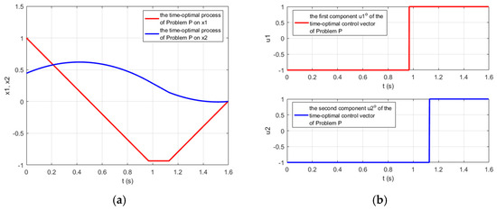
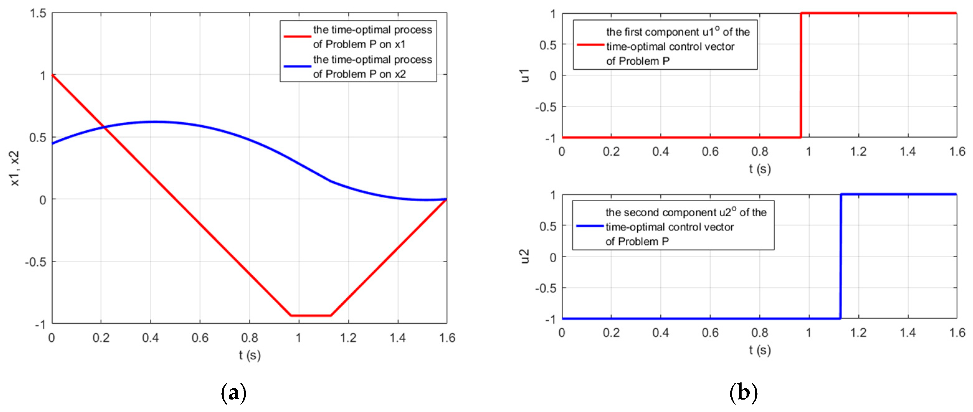
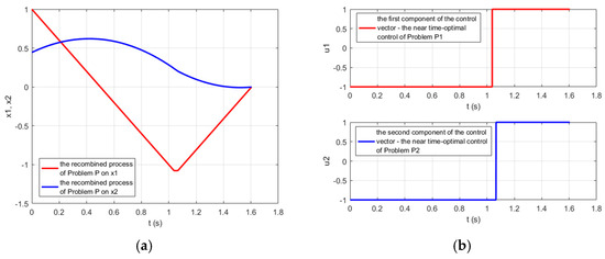
transfers the system from its initial state (93) to the state-space origin at time $t_f^{\ast }$ as shown in Figure 1.

Figure 1. The trajectory of the system (87)–(89) from its initial state (92) to the state-space origin under the control vector ${\mathit{u}}^{\ast }\left(t\right)$ (97)–(100): (a) the process regarding the state-space variables $x_1$ and $x_2$; (b) the controls $u_1^{\ast }\left(t\right)$ and $u_2^{\ast }\left(t\right)$ of the control vector ${\mathit{u}}^{\ast }\left(t\right)$.

Let us also call the above system trajectory with an initial state (93) obtained under the control vector ${\mathit{u}}^{\mathbf{\ast }}\left(t\right)$ (97)–(100) ${\mathit{x}}^{\ast }\left(t\right)$:

$$\begin{gathered} {\mathit{x}}^{\ast }\left(t\right)=e^{At}{\mathit{x}}_0+{\displaystyle \underset{0}{\overset{t}{\int }}}{e}^{A(t-\tau )}B{\mathit{u}}^{\ast }\left(\tau \right)d\tau \\ =e^{At}{\mathit{x}}_0+{\displaystyle \underset{0}{\overset{t}{\int }}}{e}^{A(t-\tau )}\left(\begin{array}{cc}{B}_1& B_2\end{array}\right)\left(\begin{array}{c}{u}_1^{\ast }\left(\tau \right)\\ u_2^{\ast }\left(\tau \right)\end{array}\right)d\tau \\ \mathrm{for} t\in \left[0, t_f^{\ast }\right], \end{gathered}$$

(101)

$$\begin{gathered} {\mathit{x}}^{\ast }\left(t\right)=e^{At}{\mathit{x}}_0+{\displaystyle \underset{0}{\overset{t}{\int }}}{e}^{A(t-\tau )}{B}_1{u}_1^{\ast }\left(\tau \right)d\tau +{\displaystyle \underset{0}{\overset{t}{\int }}}{e}^{A(t-\tau )}{B}_2{u}_2^{\ast }\left(\tau \right)d\tau \mathrm{f}\mathrm{o}\mathrm{r} t\in \left[0, t_f^{\ast }\right], \\ \mathrm{w}\mathrm{h}\mathrm{e}\mathrm{r}\mathrm{e} e^{At}=\left(\begin{array}{cc}1& 0\\ t& 1\end{array}\right), \end{gathered}$$

(102)

$${\mathit{x}}^{\ast }\left(t_f^{\ast }\right)={\mathit{x}}^{\ast }\left(1.59625\right)=\left(\begin{array}{r}1.1015\times {10}^{-16}\\ -9.7998\times {10}^{-13}\end{array}\right)\cong \left(\begin{array}{c}0\\ 0\end{array}\right).$$

(103)

We are going to show based on the PMP that ${\mathit{x}}^{\ast }\left(t\right)$ and ${\mathit{u}}^{\ast }\left(t\right)$ represent the solution of the considered time-optimal control Problem $P$. Pontryagin’s function (Hamilton function) regarding the linear time-optimal control problem represents

$$H\left(\mathit{x}\left(t\right), \mathit{u}\left(t\right),\mathit{\psi }\left(t\right)\right)={\left(\mathit{\psi }\left(t\right)\right)}^T\left(A\mathit{x}\left(t\right)+B\mathit{u}\left(t\right)\right).$$

(104)

The vector $\mathit{\psi }\left(t\right)$ represents a solution of the adjoined system

$$\dot{\mathit{\psi }}=-A^T\mathit{\psi }.$$

(105)

Its solution is

$$\begin{array}{ccc}\mathit{\psi }\left(t\right)& =& e^{-A^{T}t}{\mathit{\psi }}_0\\ & =& \left(\begin{array}{cc}1& -t\\ 0& 1\end{array}\right){\mathit{\psi }}_0.\end{array}$$

(106)

Let the initial state regarding $\mathit{\psi }$ be

$${\mathit{\psi }}_0^{\ast }={\mathit{\psi }}^{\ast }\left(0\right)=\left(\begin{array}{c}{\psi }_{10}^{\ast }\\ {\psi }_{20}^{\ast }\end{array}\right)=\left(\begin{array}{c}-882.5139\times {10}^{-3}\\ -912.1591\times {10}^{-3}\end{array}\right),$$

(107)

and consider the following solution of the adjoined system called ${\mathit{\psi }}^{\ast }(t)$:

$$\begin{gathered} {\mathit{\psi }}^{\ast }(t)=e^{-A^{T}t}{\mathit{\psi }}_0^{\ast }=\left(\begin{array}{cc}1& -t\\ 0& 1\end{array}\right)\left(\begin{array}{c}{\psi }_{10}^{\ast }\\ {\psi }_{20}^{\ast }\end{array}\right) \\ =\left(\begin{array}{c}{\psi }_{10}^{\ast }-{\psi }_{20}^{\ast }t\\ {\psi }_{20}^{\ast }\end{array}\right) \mathrm{f}\mathrm{o}\mathrm{r} t\in \left[0, t_f^{\ast }\right]. \end{gathered}$$

(108)

First, we will show that Pontryagin’s function regarding the considered Problem $P$ satisfies

$$\underset{\mathit{u}\in U}{\max } H\left({\mathit{x}}^{\ast }\left(t\right),\mathit{u}\left(t\right), {\mathit{\psi }}^{\ast }\left(t\right)\right)=H\left({\mathit{x}}^{\ast }\left(t\right),{\mathit{u}}^{\ast }\left(t\right), {\mathit{\psi }}^{\ast }\left(t\right)\right).$$

(109)

We obtain regarding $H$:

$$\begin{gathered} H\left({\mathit{x}}^{\ast }\left(t\right),\mathit{u}\left(t\right), {\mathit{\psi }}^{\ast }\left(t\right)\right)={\left({\mathit{\psi }}^{\ast }\left(t\right)\right)}^T\left(A{\mathit{x}}^{\ast }\left(t\right)+B\mathit{u}\left(t\right)\right) \\ ={\left({\mathit{\psi }}^{\ast }\left(t\right)\right)}^{T}A{\mathit{x}}^{\ast }\left(t\right)+{\left({\mathit{\psi }}^{\ast }\left(t\right)\right)}^T\left(\begin{array}{cc}{B}_1& B_2\end{array}\right)\left(\begin{array}{c}{u}_1\left(t\right)\\ u_2\left(t\right)\end{array}\right) \\ ={\left({\mathit{\psi }}^{\ast }\left(t\right)\right)}^{T}A{\mathit{x}}^{\ast }\left(t\right)+{\left({\mathit{\psi }}^{\ast }\left(t\right)\right)}^T{B}_1{u}_1\left(t\right)+{\left({\mathit{\psi }}^{\ast }\left(t\right)\right)}^T{B}_2{u}_2\left(t\right). \end{gathered}$$

(110)

$$\begin{array}{ll}H\left({\mathit{x}}^{\ast }\left(t\right),\mathit{u}\left(t\right), {\mathit{\psi }}^{\ast }\left(t\right)\right)& ={{\mathit{\psi }}^{\ast }}^T\left(t\right)A{\mathit{x}}^{\ast }\left(t\right)\\ & +{\left(\begin{array}{c}{\psi }_{10}^{\ast }-{\psi }_{20}^{\ast }t\\ {\psi }_{20}^{\ast }\end{array}\right)}^T{B}_1{u}_1\left(t\right)\\ & +{\left(\begin{array}{c}{\psi }_{10}^{\ast }-{\psi }_{20}^{\ast }t\\ {\psi }_{20}^{\ast }\end{array}\right)}^T{B}_2{u}_2\left(t\right).\end{array}$$

(111)

Let us consider the second component of the sum of $H$ (112)

$$\begin{gathered} {\left(\begin{array}{c}{\psi }_{10}^{\ast }-{\psi }_{20}^{\ast }t\\ {\psi }_{20}^{\ast }\end{array}\right)}^T{B}_1{u}_1\left(t\right)=\left(\begin{array}{cc}{\psi }_{10}^{\ast }-{\psi }_{20}^{\ast }t& {\psi }_{20}^{\ast }\end{array}\right)\left(\begin{array}{c}1\\ 0\end{array}\right)u_1\left(t\right) \\ =\left({\psi }_{10}^{\ast }-{\psi }_{20}^{\ast }t\right)u_1\left(t\right). \end{gathered}$$

(112)

The function $({\psi }_{10}^{\ast }-{\psi }_{20}^{\ast }t)$ is a linear function on $t$:

$$\left({\psi }_{10}^{\ast }-{\psi }_{20}^{\ast }t\right)=\left\{\begin{array}{ll}0& \mathrm{a}\mathrm{t} t={\displaystyle \frac{{\psi }_{10}^{\ast }}{{\psi }_{20}^{\ast }}}=0.9675=t_1^{\ast };\\ {\psi }_{10}^{\ast }=-882.5139\times {10}^{-3}<0& \mathrm{a}\mathrm{t} t=0;\\ \left({\psi }_{10}^{\ast }-{\psi }_{20}^{\ast }{t}_f^{\ast }\right)=0.57352& \mathrm{a}\mathrm{t} t=t_f^{\ast }.\end{array}\right.$$

(113)

Thus, the function $({\psi }_{10}^{\ast }-{\psi }_{20}^{\ast }t)$ is a linear increasing function switching from negative to positive values at time $t_1^{\ast }$, which is the switching moment of $u_1^{\ast }\left(t\right)$ (97), (99) as it is also shown in Figure 1b. Therefore,

$$\begin{array}{cc}\underset{\left|u_1\right|\le 1}{\max }({\psi }_{10}^{\ast }-{\psi }_{20}^{\ast }t)u_1\left(t\right)& =({\psi }_{10}^{\ast }-{\psi }_{20}^{\ast }t)sign({\psi }_{10}^{\ast }-{\psi }_{20}^{\ast }t)\\ & =\left({\psi }_{10}^{\ast }-{\psi }_{20}^{\ast }t\right)u_1^{\ast }\left(t\right). \end{array}$$

(114)

Similarly, we obtain for the third component of the sum of $H$ (112):

$$\begin{gathered} {\left(\begin{array}{c}{\psi }_{10}^{\ast }-{\psi }_{20}^{\ast }t\\ {\psi }_{20}^{\ast }\end{array}\right)}^T{B}_2{u}_2\left(t\right)=\left(\begin{array}{cc}{\psi }_{10}^{\ast }-{\psi }_{20}^{\ast }t& {\psi }_{20}^{\ast }\end{array}\right)\left(\begin{array}{c}1\\ b_{22}\end{array}\right)u_2\left(t\right) \\ =\left({\psi }_{10}^{\ast }-{\psi }_{20}^{\ast }t+{\psi }_{20}^{\ast }{b}_{22}\right)u_2\left(t\right). \end{gathered}$$

(115)

The function $({\psi }_{10}^{\ast }+{\psi }_{20}^{\ast }{b}_{22}-{\psi }_{20}^{\ast }t)$ is a linear function on $t$:

$$\begin{gathered} ({\psi }_{10}^{\ast }+{\psi }_{20}^{\ast }{b}_{22}-{\psi }_{20}^{\ast }t) \\ =\left\{\begin{array}{ll}0& \mathrm{a}\mathrm{t} t={\displaystyle \frac{{\psi }_{10}^{\ast }+{\psi }_{20}^{\ast }{b}_{22}}{{\psi }_{20}^{\ast }}}=1.1287=t_2^{\ast };\\ {\psi }_{10}^{\ast }+{\psi }_{20}^{\ast }{b}_{22}=-1.0296<0& \mathrm{a}\mathrm{t} t=0;\\ {\psi }_{10}^{\ast }+{\psi }_{20}^{\ast }{b}_{22}-{\psi }_{20}^{\ast }{t}_f^{\ast }=0.42648& \mathrm{a}\mathrm{t} t=t_f^{\ast }.\end{array}\right. \end{gathered}$$

(116)

Thus, the function $({\psi }_{10}^{\ast }+{\psi }_{20}^{\ast }{b}_{22}-{\psi }_{20}^{\ast }t)$ is a linear increasing function switching from negative to positive values at time $t_2^{\ast }$, which is the switching moment of $u_2^{\ast }\left(t\right)$ (98), (99) as it is also shown in Figure 1b. Therefore,

$$\begin{array}{l}\underset{\left|u_2\right|\le 1}{\max }({\psi }_{10}^{\ast }+{\psi }_{20}^{\ast }{b}_{22}-{\psi }_{20}^{\ast }t)u_2\left(t\right)\\ \begin{array}{l}=\left({\psi }_{10}^{\ast }+{\psi }_{20}^{\ast }{b}_{22}-{\psi }_{20}^{\ast }t\right)sign\left({\psi }_{10}^{\ast }+{\psi }_{20}^{\ast }{b}_{22}-{\psi }_{20}^{\ast }t\right)\\ =\left({\psi }_{10}^{\ast }+{\psi }_{20}^{\ast }{b}_{22}-{\psi }_{20}^{\ast }t\right)u_2^{\ast }\left(t\right).\end{array}\end{array}$$

(117)

As a result, we obtain:

$$\begin{array}{ll}\underset{\mathit{u}\in U}{\max } H\left({\mathit{x}}^{\ast }\left(t\right),\mathit{u}\left(t\right), {\mathit{\psi }}^{\ast }\left(t\right)\right)& ={\left({\mathit{\psi }}^{\ast }\left(t\right)\right)}^{T}A{\mathit{x}}^{\ast }\left(t\right)\\ & +\underset{\left|u_1\right|\le 1}{\max }{\left(\begin{array}{c}{\psi }_{10}^{\ast }-{\psi }_{20}^{\ast }t\\ {\psi }_{20}^{\ast }\end{array}\right)}^T{B}_1{u}_1\left(t\right)\\ & +\underset{\left|u_2\right|\le 1}{\max }{\left(\begin{array}{c}{\psi }_{10}^{\ast }-{\psi }_{20}^{\ast }t\\ {\psi }_{20}^{\ast }\end{array}\right)}^T{B}_2{u}_2\left(t\right);\end{array}$$

(118)

$$\begin{array}{ll}\underset{\mathit{u}\in U}{\max } H\left({\mathit{x}}^{\ast }\left(t\right),\mathit{u}\left(t\right), {\mathit{\psi }}^{\ast }\left(t\right)\right)& ={\left({\mathit{\psi }}^{\ast }\left(t\right)\right)}^{T}A{\mathit{x}}^{\ast }\left(t\right)\\ & +\underset{\left|u_1\right|\le 1}{\max }({\psi }_{10}^{\ast }-{\psi }_{20}^{\ast }t)u_1\left(t\right)\\ & +\underset{\left|u_2\right|\le 1}{\max }({\psi }_{10}^{\ast }+{\psi }_{20}^{\ast }{b}_{22}-{\psi }_{20}^{\ast }t)u_2\left(t\right);\end{array}$$

(119)

$$\begin{array}{ll}\underset{\mathit{u}\in U}{\max } H\left({\mathit{x}}^{\ast }\left(t\right),\mathit{u}\left(t\right), {\mathit{\psi }}^{\ast }\left(t\right)\right)& ={\left({\mathit{\psi }}^{\ast }\left(t\right)\right)}^{T}A{\mathit{x}}^{\ast }\left(t\right)\\ & +\left({\psi }_{10}^{\ast }-{\psi }_{20}^{\ast }t\right)u_1^{\ast }\left(t\right)\\ & +\left({\psi }_{10}^{\ast }+{\psi }_{20}^{\ast }{b}_{22}-{\psi }_{20}^{\ast }t\right)u_2^{\ast }\left(t\right)\\ & ={\left({\mathit{\psi }}^{\ast }\left(t\right)\right)}^{T}A{\mathit{x}}^{\ast }\left(t\right)+{\left({\mathit{\psi }}^{\ast }\left(t\right)\right)}^{T}B{\mathit{u}}^{\ast }\left(t\right)\\ & =H\left({\mathit{x}}^{\ast }\left(t\right),{\mathit{u}}^{\ast }\left(t\right), {\mathit{\psi }}^{\ast }\left(t\right)\right).\end{array}$$

(120)

We also obtain for $H\left({\mathit{x}}^{\ast }\left(t\right),{\mathit{u}}^{\ast }\left(t\right), {\mathit{\psi }}^{\ast }\left(t\right)\right)$ at $t=t_f^{\ast }$ from (114) and (117):

$$\begin{array}{ll}H\left({\mathit{x}}^{\ast }\left(t_f^{\ast }\right),{\mathit{u}}^{\ast }\left(t_f^{\ast }\right), {\mathit{\psi }}^{\ast }\left(t_f^{\ast }\right)\right)& ={\left({\mathit{\psi }}^{\ast }\left(t_f^{\ast }\right)\right)}^{T}A{\mathit{x}}^{\ast }\left(t_f^{\ast }\right)\\ & +\left({\psi }_{10}^{\ast }-{\psi }_{20}^{\ast }{t}_f^{\ast }\right)u_1^{\ast }\left(t_f^{\ast }\right)\\ & \begin{array}{l}+\left({\psi }_{10}^{\ast }+{\psi }_{20}^{\ast }{b}_{22}-{\psi }_{20}^{\ast }{t}_f^{\ast }\right)u_2^{\ast }\left(t_f^{\ast }\right)\\ =0+0.57352+0.42648\\ =1.\end{array}\end{array}$$

(121)

Thus, we have just shown that the control vector ${\mathit{u}}^{\mathbf{\ast }}\left(t\right)$ (97)–(100) and the respective system trajectory ${\mathit{x}}^{\ast }\left(t\right)$ (101) with an initial state (93) satisfy the PMP with respect to the considered linear time-optimal control Problem $P$. Taking into account that the PMP with respect to the linear time-optimal control problem, in case the system satisfies the condition of normality, is not only a necessary but also a sufficient condition for optimality, we can conclude that the control vector ${\mathit{u}}^{\mathbf{\ast }}\left(t\right)$ (97)–(100) and the system trajectory ${\mathit{x}}^{\ast }\left(t\right)$ (101) reaching the state-space origin at time $t_f^{\ast }$ (99) represent the only time-optimal solution to the considered Problem $P$.

3.2. A Near-Time-Optimal Control Solution of Problem $P$ Based on the Proposed Idea

Let us now try to solve the considered Problem $P$, based on the proposed idea, through the solutions of the two single-input problems—Problem $P_1$ and Problem $P_2$, obtained through the proposed decomposition of the initial Problem $P$. First, let us suppose $k$ is a positive parameter $0<k<1$.

The system of the first Problem $P_1$ is composed of the matrices $A$ and $B_1$ (89) and represents

$${\dot{\mathit{x}}}_1=\mathrm{A}{\mathit{x}}_1+B_1{u}_1.$$

(122)

The initial state of the system is

$${\mathit{x}}_1\left(0\right)={\mathit{x}}_{01}={\left(\begin{array}{cc}{x}_{10,1}& x_{10,2}\end{array}\right)}^T,$$

(123)

$${\mathit{x}}_{01}=k{\mathit{x}}_0.$$

(124)

The admissible control $u_1$ is yet defined above, a piecewise continuous function $u_1\left(t\right)$, which takes its values from the range (90), and for whom at the points of discontinuity ${\tau }_{1i}$ we have (8).

The target state at the final time $t_{1f}$, where $t_{1f}$ is unspecified, represents the origin of the system’s state-space

$${{\mathit{x}}_1\left(t_{1f}\right)=\mathit{x}}_{1f}={\left(0\right)}_{n\times 1}.$$

(125)

The time-optimal Problem $P_1$ is to find an admissible control $u_1\left(t\right)$ which transfers the system (122) from its initial state (123)–(124) to the final state (125) in minimum time, i.e., minimizing the performance index

$$J_1=t_{1f}\to min.$$

(126)

Let us formulate in the same manner the second single-input linear time-optimal control Problem $P_2$. The system is composed of the matrices $A$ and $B_2$ (89) and represents the equations

$${\dot{\mathit{x}}}_2=\mathrm{A}{\mathit{x}}_2+B_2{u}_2.$$

(127)

The initial state of the system is

$${\mathit{x}}_2\left(0\right)={\mathit{x}}_{02}={\left(\begin{array}{cc}{x}_{20,1}& x_{20,2}\end{array}\right)}^T,$$

(128)

$${\mathit{x}}_{02}=\left(1-k\right){\mathit{x}}_0.$$

(129)

The admissible control $u_2$ is yet defined above, a piecewise continuous function $u_2\left(t\right).$ It takes its values from the range (91) and at the points of discontinuity ${\tau }_{2j}$ we have (9).

The target state at the final time $t_{2f}$, where $t_{2f}$ is unspecified, represents the origin of the system’s state-space

$${{\mathit{x}}_2\left(t_{2f}\right)=\mathit{x}}_{2f}={\left(0\right)}_{n\times 1}.$$

(130)

The time-optimal Problem $P_2$ is to find an admissible control $u_2\left(t\right)$ which transfers the system (127) from its initial state (128)–(129) to the final state (130) in minimum time, i.e., minimizing the performance index

$$J_2=t_{2f}\to min.$$

(131)

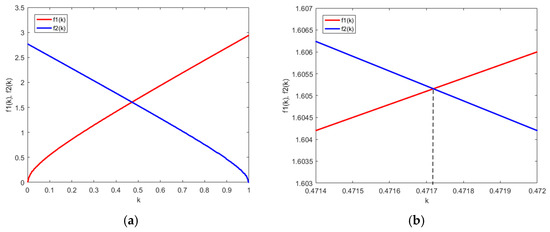
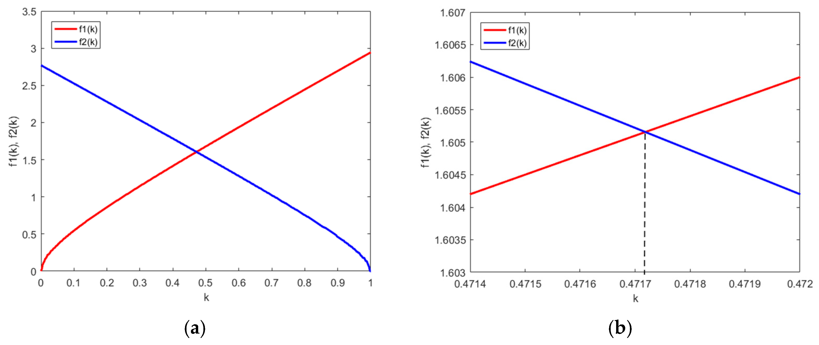
In order to illustrate Lemma 1 with respect to the example, the two continuous functions $f_1\left(k\right)$ and $f_2\left(k\right)$ (57) defined on the same interval $k\in \left[0, 1\right]$ are presented in Figure 2. $f_1\left(k\right)$ is with Problem $P_1$ while $f_2\left(k\right)$ is with Problem $P_2$. $f_1\left(k\right)$ is a continuously increasing function while $f_2\left(k\right)$ is a continuously decreasing function as shown in the derivation of Lemma 1, where

Figure 2. The two continuous functions $f_1\left(k\right)$ and $f_2\left(k\right)$ (57) defined on the same interval $k\in \left[0, 1\right]$ regarding the considered two-input double integrator system and illustrating Lemma 1: (a) $f_1\left(k\right)$ and $f_2\left(k\right)$ (57) on the whole interval $k\in \left[0, 1\right]$; (b) the magnified area around the intersection point of $f_1\left(k\right)$ and $f_2\left(k\right)$ at $k^o=0.47167$ (134). The vertical dashed line goes through the crossing point of $f_1\left(k\right)$ and $f_2\left(k\right)$ and the point at $k^o=0.47167$ of the horizontal axis.

-

$f_1\left(0\right)=0$ is the minimum time of Problem $P_1$ when ${\mathit{x}}_{01}={\mathit{x}}_0=\left(\begin{array}{c}0\\ 0\end{array}\right)$, while $f_1\left(1\right)$ is the minimum time of Problem $P_1$ when ${\mathit{x}}_{01}={\mathit{x}}_0=\left(\begin{array}{c}1\\ 0.44447\end{array}\right)$ (92), (124):

$$f_1\left(1\right)=2.94375 \left(s\right);$$

(132)

-

$f_2\left(0\right)$ is the minimum time of Problem $P_2$ when ${\mathit{x}}_{01}={(1-0)\mathit{x}}_0=\left(\begin{array}{c}1\\ 0.44447\end{array}\right)$ (92), (129):

$$f_2\left(0\right)=2.77 \left(s\right);$$

(133)

-

$f_2\left(1\right)=0$ is the minimum time of Problem $P_2$ when ${\mathit{x}}_{01}={(1-1)\mathit{x}}_0=\left(\begin{array}{c}0\\ 0\end{array}\right)$.

The area around the intersection point of $f_1\left(k\right)$ and $f_2\left(k\right)$ is magnified and shown in Figure 2b.

It should be noted that there is no practical need to obtain the whole picture of the dependence of $f_1\left(k\right)$ and $f_2\left(k\right)$ on the parameter $k$ and reveal the intersection point at $k^o$ except for the methodological point of view. In fact, several iterations on the positive number $k$, $0<k<1$, have to be made solving Problem $P_1$ and Problem $P_2$ with respective initial conditions ${\mathit{x}}_{01}$ of Problem $P_1$ and ${\mathit{x}}_{02}$ of Problem $P_2$. A short algorithmic description of the iterative procedure could be presented as follows.

Step 1: Define a desired accuracy regarding the difference between the minimum times $t_{1f}$ and $t_{2f}$;

Step 2: Choose initial $k$, $k\in \left(0, 1\right)$;

Step 3: Solve Problem $P_1$ and Problem $P_2$;

Step 3: Compare the two times $t_{1f}$ and $t_{2f}$ and obtain the ratio ${\displaystyle \frac{t_{1f}}{t_{2f}}}$;

Step 4: Increase or decrease $k$ according to the ratio ${\displaystyle \frac{t_{1f}}{t_{2f}}}$ or use bisection (or secant) to find $k$ such that $\left|t_{1f}\left(k\right)-t_{2f}\left(k\right)\right|$ is less than or equal to the desired accuracy.

The obtained final value of $k$ with an accuracy of $1\times {10}^{-6} \left(s\right)$ regarding the minimum times $t_{1f}^o$ of Problem $P_1$ and $t_{2f}^o$ of Problem $P_2$ is

$$k^o=0.47167.$$

(134)

The respective initial condition ${\mathit{x}}_{01}$ (124) of Problem $P_1$ and ${\mathit{x}}_{02}$ (129) of Problem $P_2$ at $k^o=0.47167$ are:

$${\mathit{x}}_{01}=k^o{\mathit{x}}_0=0.47167\left(\begin{array}{c}1\\ 0.44447\end{array}\right)=\left(\begin{array}{c}0.47167\\ 0.20964\end{array}\right),$$

(135)

$${\mathit{x}}_{02}=\left(1-k^o\right){\mathit{x}}_0=\left(1-0.47167\right)\left(\begin{array}{c}1\\ 0.44447\end{array}\right)=\left(\begin{array}{c}0.52833\\ 0.23483\end{array}\right),$$

(136)

and the obtained equal minimum times $t_{1f}^o$ and $t_{2f}^o$ are

$$t_{1f}^o=t_{2f}^o=1.605 \left(s\right).$$

(137)

Let $t_f^{\ast }$ be

$$t_f^{\ast }=t_{1f}^o=t_{2f}^o=1.605 \left(s\right).$$

(138)

Problem $P_1$ and Problem $P_2$ have been solved numerically by the technique in [18,19], following [18] (Section 3.2, pp. 9–13) and [19] (Section 4.1 Example 1, pp. 18–24). Both papers in [18,19] unveil new state-space properties of the linear time-optimal control problem with one input and real non-positive eigenvalues of the system following from the PMP. It is shown there that the positive semi-axis ${\mathrm{O}x}_n$ of the system of order $n$ is outside the switching hyper-surface of the considered problem, being wholly below or wholly above the switching hyper-surface of the problem, while the negative semi-axis ${\mathrm{O}x}_n$ is outside the switching hyper-surface of the considered problem, being wholly below or wholly above the switching hyper-surface but in the opposite relation to the switching hyper-surface of the problem relative to the positive semi-axis ${\mathrm{O}x}_n.$ The determination of this relation regarding the considered problem is called “axes initialization”. Here for both Problem $P_1$ and Problem $P_2$ the same result is obtained

$$x_{2+}=-1,$$

(139)

which means that all the points of the negative semi-axis ${\mathrm{O}x}_2$ of the system of Problem $P_1$ are above the switching curve, and the time-optimal control value for them is ${+u}_{1max }$. The same is true for the negative semi-axis ${\mathrm{O}x}_2$ of the system of Problem $P_2$, and the time-optimal control value for all the points of this semi-axis is ${+u}_{2max }$. Based on the properties regarding the axes initialization and discovered in [18,19], other new properties, a foundation of a new method for synthesizing the time-optimal control without the need to describe the switching hyper-surfaces, are obtained and illustrated by the examples mentioned above.

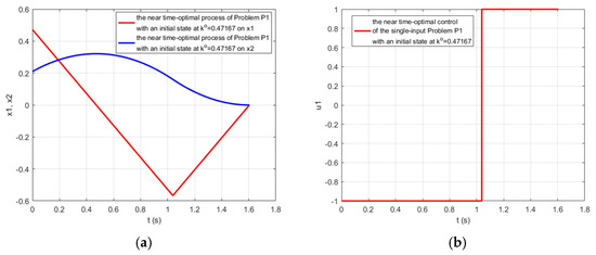
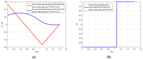
Table 1 represents, in its first row, the near-optimal solution of Problem $P_1$ with an initial state ${\mathit{x}}_{01}$ (135) and the obtained corresponding control function $u_1^{\tilde{o}}\left(t\right)$ associated with this problem. The near-optimal solution of Problem $P_2$ with an initial state ${\mathit{x}}_{02}$ (136) and the obtained corresponding control function $u_2^{\tilde{o}}\left(t\right)$ associated with this problem is presented in the second row of Table 1. The corresponding processes were obtained with an accuracy of ${\epsilon }_r=0.0006$ regarding Problem $P_1$ under $u_1^{\tilde{o}}\left(t\right)$ and Problem $P_2$ under $u_2^{\tilde{o}}\left(t\right)$, and are shown in Figure 3 and Figure 4.

Table 1. Results of the solutions of Problem $P_1$ with an initial state ${\mathit{x}}_{01}$ (135) and Problem $P_2$ with an initial state and ${\mathit{x}}_{02}$ (136) obtained with an accuracy of ${\epsilon }_r=0.0006$ satisfying Lemma 1 at $k^o=0.47167$ (134) with an accuracy of $1\times {10}^{-6} \left(s\right)$.

Problem	Control	Control in the First Interval	Switching Time ${\mathit{t}}_{\mathit{i}1}$ (s)	Control in the Second Interval	Minimum Time ${\mathit{t}}_{\mathit{f}}^{\ast }$ (s)
$P_1$	$u_1$	$-1$	$1.038333$	$1$	$1.605$
$P_2$	$u_2$	$-1$	$1.066667$	$1$	$1.605$

Figure 3. Near-time-optimal process of the system (122) of Problem $P_1$ from its initial state ${\mathit{x}}_{01}$ (135) at $k^o=0.47167$ (134) to the state-space origin obtained with an accuracy of ${\epsilon }_r=0.0006$: (a) the process regarding the state-space variables $x_1$ and $x_2$; (b) the corresponding near time-control $u_1^{\tilde{o}}\left(t\right)$ of Problem $P_1$ at $k^o=0.47167$ (134) presented in the first row of Table 1.

Figure 4. Near-time-optimal process of the system (127) of Problem $P_2$ from its initial state ${\mathit{x}}_{02}$ (136) at $k^o=0.47167$ (134) to the state-space origin obtained with an accuracy of ${\epsilon }_r=0.0006$: (a) the process regarding the state-space variables $x_1$ and $x_2$; (b) the corresponding near time-control $u_2^{\tilde{o}}\left(t\right)$ of Problem $P_2$ at $k^o=0.47167$ (134) presented in the second row of Table 1.

Let us now consider the initial Problem $P$ (87)–(94) under the control vector composed of the solutions $u_1^o\left(t\right)$ of Problem $P_1$ and $u_2^o\left(t\right)$ of Problem $P_2$ as (86), bearing in mind that $t_f^{\ast }$ represents (138),

$${\mathit{u}}^{\ast }\left(t\right)=\left(\begin{array}{c}{u}_1^o\left(t\right)\\ u_2^o\left(t\right)\end{array}\right) \mathrm{f}\mathrm{o}\mathrm{r} t\in \left[0,t_f^{\ast }\right].$$

(140)

Let the trajectory of the system of Problem $P$ be ${\mathit{x}}^{\ast }\left(t\right)$. It represents the sum of the obtained trajectories ${\mathit{x}}_1^o\left(t\right)$ of Problem $P_1$ under $u_1^o\left(t\right)$ and ${\mathit{x}}_2^o\left(t\right)$ of Problem $P_2$ under $u_2^o\left(t\right)$.

$$\begin{array}{ll}{\mathit{x}}^{\ast }\left(t\right)& =e^{At}{\mathit{x}}_0+{\displaystyle \underset{0}{\overset{t}{\int }}}{e}^{A\tau }B{\mathit{u}}^{\ast }(t-\tau )d\tau \\ & =e^{At}{\mathit{x}}_0+{\displaystyle \underset{0}{\overset{t}{\int }}}{e}^{A\tau }\left(\begin{array}{cc}{B}_1& B_2\end{array}\right)\left(\begin{array}{c}{u}_1^o\left(t-\tau \right)\\ u_2^o\left(t-\tau \right)\end{array}\right)d\tau \\ & =e^{At}{k}^o{\mathit{x}}_0+e^{At}\left(1-k^o\right){\mathit{x}}_0+{\displaystyle \underset{0}{\overset{t}{\int }}}{e}^{A\tau }{B}_1{u}_1^o\left(t-\tau \right)d\tau +{\displaystyle \underset{0}{\overset{t}{\int }}}{e}^{A\tau }{B}_2{u}_2^o\left(t-\tau \right)d\tau .\end{array}$$

(141)

$$\begin{array}{cc}{\mathit{x}}^{\ast }\left(t\right)& =e^{At}{k}^o{\mathit{x}}_0+{\displaystyle \underset{0}{\overset{t}{\int }}}{e}^{A\tau }{B}_1{u}_1^o\left(t-\tau \right)d\tau +e^{At}\left(1-k^o\right){\mathit{x}}_0+{\displaystyle \underset{0}{\overset{t}{\int }}}{e}^{A\tau }{B}_2{u}_2^o\left(t-\tau \right)d\tau \\ & \mathrm{f}\mathrm{o}\mathrm{r}t\in \left[0, t_f^o\right].\end{array}$$

(142)

$$\begin{array}{l}{\mathit{x}}^{\ast }\left(t\right)={\mathit{x}}_1^o\left(t\right)+{\mathit{x}}_2^o\left(t\right) \mathrm{f}\mathrm{o}\mathrm{r} t\in \left[0, t_f^o\right],\\ {\mathit{x}}_1^o\left(t\right)=e^{At}{k}^o{\mathit{x}}_0+{\displaystyle \underset{0}{\overset{t}{\int }}}{e}^{A\tau }{B}_1{u}_1^o\left(t-\tau \right)d\tau ,\\ {\mathit{x}}_2^o\left(t\right)=e^{At}(1-k^o){\mathit{x}}_0+{\displaystyle \underset{0}{\overset{t}{\int }}}{e}^{A\tau }{B}_2{u}_2^o\left(t-\tau \right).\end{array}$$

(143)

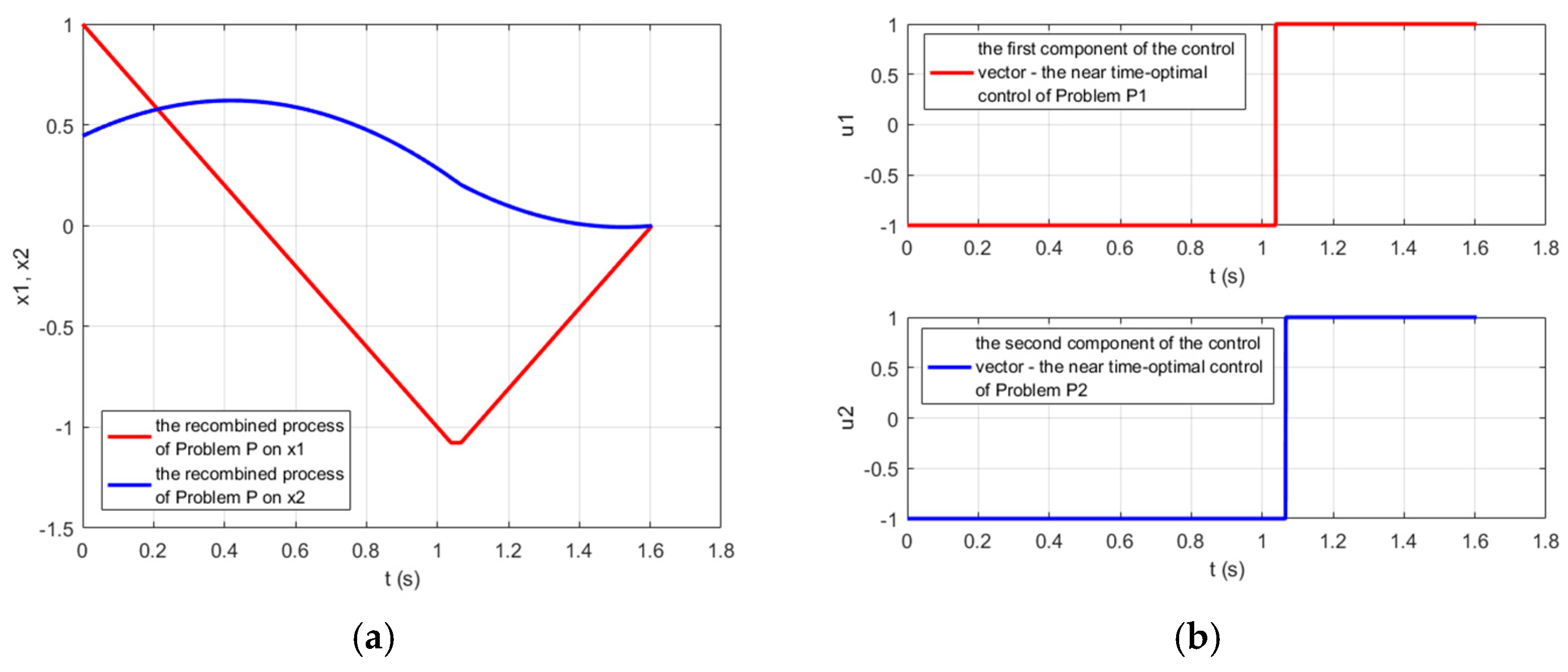
The trajectory ${\mathit{x}}^{\ast }\left(t\right)$ and the control vector ${\mathit{u}}^{\ast }\left(t\right)$ regarding the processes of the system of Problem $P$ are shown in Figure 5. The parameters of the components $u_1^{\tilde{o}}\left(t\right)$ and $u_1^{\tilde{o}}\left(t\right)$ of ${\mathit{u}}^{\ast }\left(t\right)$ (140) are presented in Table 1.

Figure 5. The trajectory ${\mathit{x}}^{\ast }\left(t\right)$ of the system (87)–(89) of Problem $P$ from its initial state ${\mathit{x}}_0$ (92) to the state-space origin obtained with an accuracy of ${\epsilon }_r=0.001$ under the control vector ${\mathit{u}}^{\ast }\left(t\right)$ (140): (a) the process regarding the state-space variables $x_1$ and $x_2$; (b) the components of the near-time-optimal controls $u_1^{\tilde{o}}\left(t\right)$ and $u_2^{\tilde{o}}\left(t\right)$ of the recombined control vector ${\mathit{u}}^{\ast }\left(t\right)$ (140) with parameters presented in Table 1.

Even though the only time-optimal solution of Problem $P$ is found in the previous Section 3.1, let us apply Theorem 1 regarding the control vector function (86), which is obtained here regarding the considered example control vector function (140), and consider it as a candidate for the solution to the original time-optimal control Problem $P$ with an initial state ${\mathit{x}}_0$ (92) according to Lemma 1. We must check the consistency of the linear system (78), (79), and (82). According to the data in Table 1, the number of switchings of $u_1^o\left(t\right)$ is $k_1=1$, and the number of switchings of $u_2^o\left(t\right)$ is $k_2=1$. Equation (78) represents

$${B_1}^T{e}^{-A^T{t}_{11}}{\mathit{\psi }}_0^{\ast }=0.$$

(144)

$$\left(\begin{array}{cc}1& 0\end{array}\right)\left(\begin{array}{cc}1& -t_{11}\\ 0& 1\end{array}\right)\left(\begin{array}{c}{\psi }_{10}^{\ast }\\ {\psi }_{20}^{\ast }\end{array}\right)=0.$$

(145)

$$\left(\begin{array}{cc}1& -t_{11}\end{array}\right)\left(\begin{array}{c}{\psi }_{10}^{\ast }\\ {\psi }_{20}^{\ast }\end{array}\right)=0.$$

(146)

Equation (79) represents

$${B_2}^T{e}^{-A^T{t}_{21}}{\mathit{\psi }}_0^{\ast }=0.$$

(147)

$$\left(\begin{array}{cc}1& 0.1612\end{array}\right)\left(\begin{array}{cc}1& -t_{21}\\ 0& 1\end{array}\right)\left(\begin{array}{c}{\psi }_{10}^{\ast }\\ {\psi }_{20}^{\ast }\end{array}\right)=0.$$

(148)

$$\left(\begin{array}{cc}1& 0.1612-t_{21}\end{array}\right)\left(\begin{array}{c}{\psi }_{10}^{\ast }\\ {\psi }_{20}^{\ast }\end{array}\right)=0.$$

(149)

Equation (82) represents

$$\left(u_1^o\left(t_f^{\ast }\right){B_1}^T{e}^{-A^T{t}_f^{\ast }}+u_2^o\left(t_f^{\ast }\right){B_2}^T{e}^{-A^T{t}_f^{\ast }}\right){\mathit{\psi }}_0^{\ast }=1.$$

(150)

$$\left(\left(\begin{array}{cc}1& -t_f^{\ast }\end{array}\right)+\left(\begin{array}{cc}1& 0.1612-t_f^{\ast }\end{array}\right)\right)\left(\begin{array}{c}{\psi }_{10}^{\ast }\\ {\psi }_{20}^{\ast }\end{array}\right)=1.$$

(151)

$$\left(\begin{array}{cc}2& 0.1612-2t_f^{\ast }\end{array}\right)\left(\begin{array}{c}{\psi }_{10}^{\ast }\\ {\psi }_{20}^{\ast }\end{array}\right)=1.$$

(152)

Thus, the linear system (78), (79), and (82), consisting here according to (83) of

$$m=k_1+k_2+1=1+1+1=3$$

(153)

equations, represents

$$\left(\begin{array}{cc}1& -t_{11}\\ 1& 0.1612-t_{21}\\ 2& 0.1612-2t_f^{\ast }\end{array}\right)\left(\begin{array}{c}{\psi }_{10}^{\ast }\\ {\psi }_{20}^{\ast }\end{array}\right)=\left(\begin{array}{c}0\\ 0\\ 1\end{array}\right).$$

(154)

According to Table 1, $t_{11}=1.038333$, $t_{21}=1.066667$, and $t_f^{\ast }=1.605$. Thus, the coefficient matrix and the augmented matrix of the above linear system are:

$$\left(\begin{array}{cc}1& -1.0383\\ 1& -0.90547\\ 2& -3.0488\end{array}\right),$$

(155)

$$\left(\begin{array}{cc}1& -1.0383\\ 1& -0.90547\\ 2& -3.0488\end{array}|\begin{array}{c}0\\ 0\\ 1\end{array}\right).$$

(156)

The ranks of the above matrices (155) and (156) differ

$$rank\left(\begin{array}{cc}1& -1.0383\\ 1& -0.90547\\ 2& -3.0488\end{array}\right)=2\ne rank\left(\begin{array}{cc}1& -1.0383\\ 1& -0.90547\\ 2& -3.0488\end{array}|\begin{array}{c}0\\ 0\\ 1\end{array}\right)=3,$$

(157)

and according to the Kronecker-Capelli Theorem, the considered linear system with unknowns ${\psi }_{10}^{\ast }$ and ${\psi }_{20}^{\ast }$ has no solution, i.e., is inconsistent. Thus, according to Theorem 1 the control vector function obtained by the proposed method (140) can only be considered as a somewhat near-time-optimal control solution to the problem considered in this example $P$.

3.3. A Comparison Between the Time-Optimal and the Obtained Near-Time-Optimal Solution of Problem $P$

Let us first make a quality assessment of the obtained solutions of Problem $P.$ The presented time-optimal solution in Section 3.1 fully complies with the PMP. According to the formulation of Problem $P$ the two-input system satisfies the condition of normality being controllable on each input. The allowable control set $U$ is convex since it represents a square with side $1$ in the plane $u_1{u}_2$. It is also symmetric where the origin $0$ of the plane $u_1{u}_2$ is an inner point and the center of $U$. Hence, regarding the linear time-optimal control problem, the PMP is a necessary and sufficient condition of optimality. The minimum time is achieved through a bang-bang control regarding each of the two components $u_1$ and $u_2$ of the control vector, i.e., the values of the control vector function are taken only at the vertices of the square $U$. The sequence of the vertices of the square $U$ that the time-optimal control vector ${\mathit{u}}^{\mathbf{\ast }}\left(t\right)$ (97)–(100) follows is

$$\left\{\left(-1,-1\right),\left(+1,-1\right),\left(+1,+1\right)\right\}$$

(158)

as shown in Figure 1b.

The obtained near-time-optimal solution also achieved a trajectory with an end in the state-space $O$ of the plane $x_1{x}_2$ but with an accuracy of ${\epsilon }_r=0.001$, obtained at the corresponding control vector (140) with values taken also exclusively at the vertices of the square $U$. The sequence of the vertices of the square $U$ that the near-time-optimal control vector ${\mathit{u}}^{\mathbf{\ast }}\left(t\right)$ (140) follows is the same time-optimal control sequence (158) of the vertices of the square $U$, as shown in Table 1 and Figure 5b.

A quantitative comparison between the time-optimal and the obtained near-time-optimal process is presented in Table 2. It is noticed that the switching times of the true time-optimal process regarding the optimal control functions $u_1\left(t\right)$ and $u_2\left(t\right)$ differ. Although this fact raises an initial bewilderment, the PMP does not require satisfying identical switching times regarding the allowable set of controls. The switching times are determined by the condition (109), which does not require exclusively identical switching times for all control functions composing the control vector function of the system. Even though the switching times of the obtained near-time-optimal solution regarding the controls $u_1$ and $u_2$, compared to the corresponding time-optimal switching times of the controls $u_1$ and $u_2$, show light mismatches, the near-time-optimal solution achieves a transition time only slightly longer than the time-optimal transition time with a relative error of less than $0.55\%$.

Table 2. A quantitative comparison between the true time-optimal and the near-time-optimal solution of Problem $P$ obtained by the proposed method.

Quantity (s)	True Time-Optimal Control (s)	Proposed Method (s)	Absolute Error (s)	Relative Error $\%$
Final time	$1.59625$	$1.605$	$+0.00875$	$0.54816$
Switching time $\mathrm{regarding} u_1$	$0.9675$	$1.038333$	$+0.070833$	$7.3212$
Switching time $\mathrm{regarding} u_2$	$1.1287$	$1.066667$	$-0.062033$	$5.496$

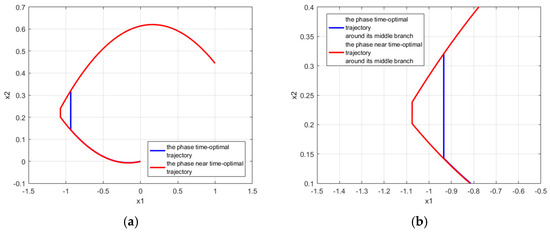
The phase trajectories in the phase-plane $x_1{x}_2$ regarding the time-optimal and the obtained near-time-optimal solution are compared in Figure 6a. It can be noticed that the first and the last third parts of the time-optimal and near-time-optimal trajectory practically coincide. The first branch of each of the two trajectories corresponds to the vertex $\left(-1,-1\right)$ of the square $U$, the middle branch corresponds to the vertex $\left(+1,-1\right)$, and the last third branch corresponds to the vertex $\left(+1,+1\right)$ of the square $U$. There is a small mismatch in the area where the switchings regarding the two controls occur, which corresponds to the middle part of the phase trajectory. The length of the middle branch of each of the two trajectories represents the time interval between the switching of $u_1$ and the switching of $u_2$ regarding the near-time-optimal and the true time-optimal process, respectively. The duration of this branch is shorter at the near-time-optimal process than the duration of the second branch of the true time-optimal process

$$\left(1.066667-1.038333\right)<\left(1.1287-0.9675\right),$$

(159)

while the duration of the first branch of the near-time-optimal trajectory is longer than the true time-optimal one—$1.038333 \left(s\right)$ against $0.9675 \left(s\right)$, which may result in a longer transition time of the near-time-optimal process. This is partly offset by an earlier jump to the third branch of the trajectory by the near-time-optimal control. Thus, the transition time under the near-time-optimal control is slightly longer than that of the time-optimal transition. The relative error is only $0.55\%$.

Figure 6. A comparison between the true time-optimal and the near-time-optimal solution of Problem $P$ obtained by the proposed method: (a) the phase time-optimal trajectory marked with blue in the plane $x_1{x}_2$ compared to the phase near the time-optimal trajectory marked with red; (b) the magnified area in the phase plane $x_1{x}_2$ around the middle branch of the trajectory, where a small mismatch in the switching times occurs.

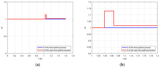
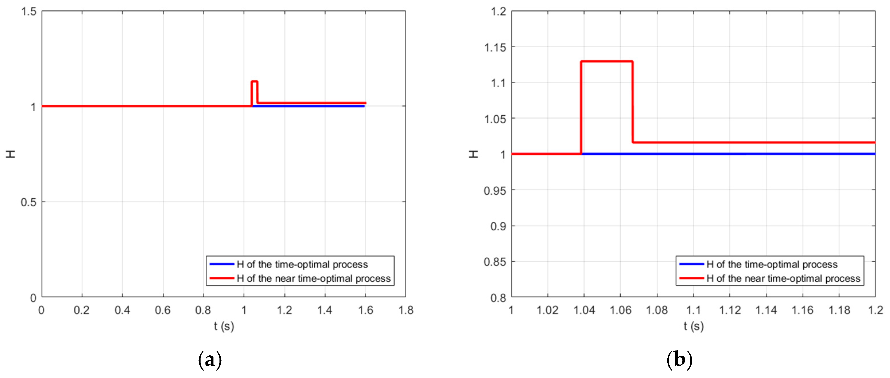
Figure 7 shows Pontryagin’s function

$$H\left({\mathit{x}}^{\ast }\left(t\right),{\mathit{u}}^{\ast }\left(t\right), {\mathit{\psi }}^{\ast }\left(t\right)\right) \mathrm{f}\mathrm{o}\mathrm{r} t\in \left[0, t_f^{\ast }\right], t_f^{\prime }=1.59625\left(s\right),$$

(160)

of the time-optimal process, marked with blue. It is compared with the function

$$H\left({\mathit{x}}^{\ast }\left(t\right),{\mathit{u}}^{\ast }\left(t\right), {\mathit{\psi }}^{\ast }\left(t\right)\right) \mathrm{f}\mathrm{o}\mathrm{r} t\in \left[0, t_f^{\ast }\right], t_f^{\prime }=1.605 \left(s\right),$$

(161)

marked with red, where ${\mathit{x}}^{\ast }\left(t\right)$ and ${\mathit{u}}^{\ast }\left(t\right)$ are the obtained trajectory and control vector function of the near-time-optimal solution, while ${\mathit{\psi }}^{\ast }\left(t\right)$ is the solution of the adjoint system (105)–(108) regarding the time-optimal process. Until the middle part of the process, both functions have the same value. During the short middle part of the process, the second function $H$ shows a little perturbation, but after the switchings H remains constant, slightly shifted from the optimal one. From the point of view of the function $H$, acting in optimal control, the role of the performance index, the replacement of ${\mathit{x}}^{\ast }\left(t\right)$ and ${\mathit{u}}^{\ast }\left(t\right)$ with the near-time-optimal trajectory and the near-time-optimal control vector function, results in slightly less effectiveness, occurring from the beginning of the middle section until the end of the process.

Figure 7. A comparison between the true time-optimal and the near-time-optimal solution of Problem $P$ regarding $H\left({\mathit{x}}^{\ast }\left(t\right),{\mathit{u}}^{\ast }\left(t\right), {\mathit{\psi }}^{\ast }\left(t\right)\right):$ (a) $H\left({\mathit{x}}^{\ast }\left(t\right),{\mathit{u}}^{\ast }\left(t\right), {\mathit{\psi }}^{\ast }\left(t\right)\right)$ of the time-optimal process, marked with blue, compared to $H\left({\mathit{x}}^{\ast }\left(t\right),{\mathit{u}}^{\ast }\left(t\right), {\mathit{\psi }}^{\ast }\left(t\right)\right)$, marked with red, where ${\mathit{x}}^{\ast }\left(t\right)$ and ${\mathit{u}}^{\ast }\left(t\right)$ are replaced with the near-time-optimal solution, while ${\mathit{\psi }}^{\ast }\left(t\right)$ remains the solution of the adjoined system (105)–(108); (b) the magnified area regarding $H\left({\mathit{x}}^{\ast }\left(t\right),{\mathit{u}}^{\ast }\left(t\right), {\mathit{\psi }}^{\ast }\left(t\right)\right)$ around the middle branch of the trajectory, where a small mismatch in the switching times occurs.

We can resume that:

• The control obtained by the proposed method near-time-optimal control is a bang-bang control with the same qualitative structure as the time-optimal one, including the switching sequence of the control vector at the vertices of the allowable set—the square $U$.
• The time-optimal trajectory in the phase plane $x_1{x}_2$ as well as the near-time-optimal trajectory comprises three branches. The major parts of the first and the last third of the time-optimal and near-time-optimal trajectory practically coincide. There is a small mismatch concerning the middle part of the phase trajectory because of the small mismatch regarding the switching times of the two control functions. Both the time-optimal and the near-time-optimal trajectories approach the state-space origin in practically the same way.
• The transition time under the near-time-optimal control is slightly longer than the time-optimal transition one. The relative error is only $0.55\%$.
• This confirms the prediction of Theorem 1.

4. Discussion and Concluding Remarks

The experimental results convincingly show that the proposed method has potential. The novelty here is that the method decomposes the initial two-input problem into two tied-together single-input problems. The first commitment is with the initial state of each one single-input problem, so that the first part of the segment with one end at the state-space origin and second end at the initial state of two-input problem defines the initial state of the first single-input problem, while the rest part of the segment defines the initial state of the second single-input problem, along with the decomposition regarding the two controls. The second commitment is with the minimum times of the solutions of both single-input problems. Here, the existence of such a point of the considered segment so that both single-input problems achieve the same minimum time according to the PMP regarding each one problem which is the point of Lemma 1, and allowance to consider the recombination of both solutions of the single-input problems as a candidate for the time-optimal solution of the initial two-input problem.

This technique could be extended to multi-input systems through dividing the above segment into parts, whose number is equal to the number of the system’s inputs, while the second commitment remains the same—achievement of identical minimum times of the solutions of all single-input problems. Satisfying the second commitment looks predictable, keeping in mind the considerations for deducing Lemma 1.

The extension of Theorem 1 in the same manner looks also predictable and could provide an easy criterion to check the optimality of the recombination of the solutions of the single-input problems.

The decomposition of the initial two-input problem is provoked by the fact that the discovered new geometric state-space properties of the single-input linear time-optimal problem [18,19], following from the PMP, provide a new time-optimal synthesis technique and obtain the minimum time solution for high-order systems [19] (Section 4.2. Example 2, pp. 25–30), while eliminating the need to construct switching hyper-surfaces. This advantage makes the idea of the decomposition of the two-input problem into two single-input problems attractive. The proposed separation is not only with respect to the controls, but also with respect to the initial state of the two-input problem, dividing it into two initial states of each one single-input problem along the ray with origin at the state-space origin and passing through the initial state of the two-input problem, on the one hand, and on the other hand, the existence of unique point at the ray that provides the same minimum times for both single-input time-optimal problems.

The combination of these theoretically backed novelties allows solving a modified canonical single-input double integrator system to a system with two independent inputs, as an example, and obtaining a near-time-optimal solution with the same qualitative structure as the time-optimal one, including the switching sequence of the control vector at the vertices of the allowable set—the square $U$, and a minimum time slightly longer than the optimal time, with a relative error of only $0.55\%$.

Continuing the reasoning towards the practical application of the presented results, attention should be paid to the fact that whenever time-optimal or bang-bang strategies are considered, high-frequency switching (chattering), especially in practical implementations where unmodeled dynamics or actuator limitations exist, may play a significant role. For this reason, some new techniques to cope with chattering could serve well, especially when they “lead to an increase in control efficiency compared with traditional sliding mode-based constrained attitude controllers without adding any computational burden” as in [16].

Further research could concern, in addition to the attempt to extend the obtained theoretical results to the general multi-input case, the derivation of a formal mathematical upper bound in case of sub-optimality, the decomposition technique regarding the separation of the initial state of the two-input problem between the initial states of the two single-input problems. This part could be further analyzed to avoid restrictive topological assumptions and configure a form of separation, achieving a guaranteed true optimal solution at the recombination of the single-input solutions.

References

- Pontryagin, L.S.; Boltyanskii, V.G.; Gamkrelidze, R.V.; Mischenko, E.F. The Mathematical Theory of Optimal Processes; Pergamon Press: Oxford, UK, 1964. [Google Scholar]
- Athans, M.; Falb, P.L. Optimal Control: An Introduction to the Theory and Its Applications; McGraw-Hill: New York, NY, USA, 1966. [Google Scholar]
- Болтянский, В.Г. Математические Методы Оптимального Управления; Наука: Moskow, Russia, 1969. [Google Scholar]
- Lee, E.B.; Markus, L. Foundations of Optimal Control Theory; Wiley & Sons Inc.: Hoboken, NJ, USA, 1967. [Google Scholar]
- Pinch, E.R. Optimal Control and the Calculus of Variations; Oxford University Press: Oxford, UK, 1993. [Google Scholar]
- Kirk, D.E. Optimal Control Theory: An Introduction; Dover Publications Inc.: Mineola, NY, USA, 2004. [Google Scholar]
- Naidu, D.S. Optimal Control Systems; CRC Press: Boca Raton, FL, USA, 2003. [Google Scholar]
- Locatelli, A. Optimal Control of a Double Integrator; Studies in Systems, Decision and Control; Springer: Cham, Switzerland, 2017; Volume 68, ISBN 978-3-319-42126-1. [Google Scholar] [CrossRef] [Scilit]
- He, S.; Hu, C.; Zhu, Y.; Tomizuka, M. Time optimal control of triple integrator with input saturation and full state constraints. Automatica 2020, 122, 109240. [Google Scholar] [CrossRef] [Scilit]
- La Valle, A.J.; Sakcak, B.; LaValle, S.M. Bang-Bang Boosting of RRTs. In Proceedings of the 2023 IEEE/RSJ International Conference on Intelligent Robots and Systems (IROS), Detroit, MI, USA, 1–5 October 2023; pp. 2869–2876. [Google Scholar] [CrossRef] [Scilit]
- Consolini, L.; Laurini, M.; Piazzi, A. Generalized Bang-Bang Control for Multivariable Feedforward Regulation. In Proceedings of the 32nd Mediterranean Conference on Control and Automation (MED), Chania, Greece, 11–14 June 2024; pp. 506–511. [Google Scholar] [CrossRef] [Scilit]
- Consolini, L.; Piazzi, A. Generalized bang-bang control for feedforward constrained regulation. Automatica 2009, 45, 2234–2243. [Google Scholar] [CrossRef] [Scilit]
- Jurdjevic, V. Geometric Control Theory; Cambridge University Press: New York, NY, USA, 1997. [Google Scholar]
- Wang, B.; Sun, J.; Peng, B.; Cui, X.; Cheng, L.; Zheng, X. Optimal Event-Triggered Neural Learning Tracking Control for Pneumatic Muscle Antagonistic Joint With Asymmetric Constraints. IEEE Trans. Ind. Electron. 2025, 72, 14677–14687. [Google Scholar] [CrossRef] [Scilit]
- Zhang, J.; Song, Y.; Zheng, G. Prescribed-time observer for descriptor systems with unknown input. Automatica 2025, 172, 111999. [Google Scholar] [CrossRef] [Scilit]
- Li, D.; Tong, S.; Yang, H.; Hu, Q. Time-Synchronized Control for Spacecraft Reorientation With Time-Varying Constraints. IEEE/ASME Trans. Mechatron. 2025, 30, 2073–2083. [Google Scholar] [CrossRef] [Scilit]
- Hu, J.; Chen, B.; Ghosh, B. Formation–Circumnavigation Switching Control of Multiple ODIN Systems via Finite-Time Intermittent Control Strategies. IEEE Trans. Control Netw. Syst. 2024, 11, 1986–1997. [Google Scholar] [CrossRef] [Scilit]
- Penev, B. One New Property of a Class of Linear Time-Optimal Control Problems. Mathematics 2023, 11, 3486. [Google Scholar] [CrossRef] [Scilit]
- Penev, B.G. Some New Geometric State-Space Properties of the Classical Linear Time-Optimal Control Problem with One Input and Real Non-Positive Eigenvalues of the System Following from Pontryagin’s Maximum Principle. Axioms 2025, 14, 97. [Google Scholar] [CrossRef] [Scilit]
Disclaimer/Publisher’s Note: The statements, opinions and data contained in all publications are solely those of the individual author(s) and contributor(s) and not of MDPI and/or the editor(s). MDPI and/or the editor(s) disclaim responsibility for any injury to people or property resulting from any ideas, methods, instructions or products referred to in the content. |
© 2026 by the author. Licensee MDPI, Basel, Switzerland. This article is an open access article distributed under the terms and conditions of the Creative Commons Attribution (CC BY) license.