


Abstract
Dynamic community detection seeks to identify changing structural groups in temporal graphs; however, current neural methodologies are susceptible to misinterpreting transient edges, noisy temporal variations, or unusual spectral disturbances as authentic structural changes. This research introduces TriMeta-BFNet, a tri-meta stacked atypical-frequency Bayesian Fourier neural network designed for hallucination-resistant community discovery. The proposed system presents a three-dimensional meta-counterbalance mechanism that includes topological consistency, Fourier-domain atypical frequency modeling, and Bayesian posterior uncertainty estimation. Initially, temporal graph signals are converted into the Fourier domain to distinguish stable low-frequency community patterns from erratic high-frequency disturbances. Secondly, unusual frequency points are detected by spectral energy deviation and integrated into a stacked neural representation module, enabling the model to differentiate significant structural alterations from extraneous oscillations. Third, Bayesian inference is employed to assess posterior uncertainty regarding community assignments, therefore mitigating overconfident predictions in the presence of ambiguous or noisy graph evolution. The three components are simultaneously optimized via a cohesive objective function that integrates community detection loss, structural consistency regularization, atypical-frequency penalty, temporal stability management, and Bayesian calibration loss. The resultant structure offers both resilient community divisions and comprehensible hallucination-risk assessments. TriMeta-BFNet theoretically conceptualizes hallucination in dynamic community detection as an imbalance of structural, spectral, and uncertainty factors, and it develops a mathematically rigorous counterbalance mechanism to mitigate erroneous community evolution. The suggested model presents a novel approach to uncertainty-aware, frequency-sensitive, and interpretable dynamic graph learning.
Keywords:
dynamic community detection; bayesian neural networks; fourier analysis; temporal graphs; hallucination-resistant learning; uncertainty quantification; spectral graph learning; atypical frequency points; graph neural networks; community evolution MSC:
68T07
1. Introduction
Community detection is a crucial issue in network science, graph mining, graph theory, and machine learning, focused on identifying groupings of nodes that exhibit denser intra-community connectivity compared to inter-community connectivity. In various real-world systems, such as social networks, financial transaction systems, biological interaction networks, transportation infrastructures, communication systems, and recommendation platforms, graph structures undergo continual evolution rather than remaining static. This presents the challenge of dynamic community detection, which aims to recognize community structures at specific timestamps while simultaneously capturing the temporal history, structural transitions, and stability features of communities during dynamic graph sequences. Recent surveys on temporal graph neural networks and dynamic graph representation learning reveal that modeling temporal dependencies, analyzing structural drift, estimating uncertainty, and conducting robust dynamic evaluations continue to pose significant challenges in contemporary graph learning systems [1,2,3].
Contemporary dynamic community identification techniques increasingly utilize graph neural networks, temporal attention mechanisms, recurrent architectures, contrastive learning, and dynamic graph embedding frameworks to represent developing structural dependencies [4,5]. While these methods enhance the capacity for temporal representation learning, their robustness is significantly affected by noisy edges, incomplete observations, transitory interactions, structural disturbances, and unstable temporal fluctuations. In practical dynamic graph contexts, a model may erroneously perceive noisy short-term fluctuations as significant community evolution, leading to unstable or too confident community transitions [6]. This phenomena is termed community detection hallucination, indicating illusory or inadequately substantiated community evolution patterns resulting from unstable temporal evidence, noisy structural observations, or inaccurately calibrated dynamic forecasts.
This issue cannot be resolved merely by enhancing temporal smoothness. Excessive smoothness may obscure authentic rapid structural shifts, whereas inadequate smoothing permits transitory perturbations and noisy interactions to prevail in community evolution patterns. Thus, hallucination-resistant dynamic community detection necessitates a technique that concurrently assesses structural consistency, spectral response, and predictive uncertainty. Fourier analysis and spectral graph learning offer a robust framework for decomposing temporal graph dynamics into frequency-domain components, facilitating the distinction between stable low-frequency structural patterns and unstable high-frequency fluctuations [7,8,9]. Nonetheless, high-frequency components cannot be eliminated indiscriminately, as they may signify either noise or significant abrupt shifts within communities. This engenders a significant ambiguity issue in dynamic graph learning: erratic high-frequency responses may indicate either illusory disturbances or genuine structural changes. Bayesian uncertainty estimate offers an alternative approach to resolving this issue. Recent studies indicate that graph neural networks often exhibit inadequate uncertainty calibration, particularly in the presence of distributional shifts, noisy relational evidence, incomplete graph observations, and dynamic structural dependencies [10,11,12]. Bayesian posterior modeling and uncertainty-aware graph learning enhance predictive reliability by recognizing overconfident predictions that lack adequate structural support. In dynamic community detection, posterior uncertainty functions as a hallucination-risk indicator, pinpointing unstable community assignments predominantly influenced by anomalous spectral fluctuations or insufficient topological evidence.
Inspired by these discoveries, this study introduces TriMeta-BFNet, a Tri-Meta Stacked Atypical-Frequency Bayesian Fourier Neural Network designed for hallucination-resistant community detection in dynamic graphs. The proposed approach presents a tri-meta counterbalance mechanism that integrates topological consistency modeling, atypical-frequency Fourier analysis, and Bayesian posterior uncertainty estimates into a cohesive optimization architecture. The topological module assesses enduring structural support for anticipated communities, the Fourier module detects anomalous frequency points via spectral-energy deviation analysis, and the Bayesian module quantifies predictive uncertainty to mitigate overconfident community transitions in ambiguous structural-frequency scenarios.
TriMeta-BFNet is predicated on the premise that illusory community evolution arises from the disparity among topology, spectral response, and uncertainty calibration. A community transition is deemed high-risk when it lacks adequate topological support, is characterized by unusual spectral variation, and displays significant posterior uncertainty concurrently. Conversely, dependable community evolution must exhibit structural consistency, comprehensible frequency-domain behavior, and consistent uncertainty calibration. The proposed framework, grounded in this principle, defines hallucination-resistant dynamic community detection as a joint optimization problem that incorporates community detection loss, topological consistency regularization, atypical-frequency penalties, temporal stability constraints, and Bayesian calibration objectives. In contrast to current dynamic graph neural networks and temporal community detection methods, TriMeta-BFNet does not depend exclusively on temporal smoothing or localized message propagation. It presents a layered Bayesian Fourier architecture wherein topology, unusual frequency response, and posterior uncertainty mutually restrict each other via tri-meta optimization. This technique enables the framework to maintain significant abrupt structural transitions while mitigating illusory community evolution induced by unstable temporal fluctuations, noisy graph connections, high-frequency disruptions, or inadequately calibrated neural predictions.
The methodological novelty of TriMeta-BFNet lies not in the individual use of Bayesian inference, Fourier-domain analysis, or graph neural architectures, but in their unified integration within a tri-meta counterbalance framework for hallucination-resistant community detection. Unlike existing approaches that typically address structural learning, spectral modeling, or uncertainty estimation separately, the proposed framework jointly evaluates persistent topological support, atypical-frequency spectral responses, and Bayesian posterior uncertainty during community evolution. By explicitly modeling the interactions among these complementary sources of evidence, TriMeta-BFNet formulates community hallucination as a reliability imbalance problem and introduces a unified optimization strategy that simultaneously promotes structural consistency, spectral stability, uncertainty calibration, and perturbation robustness. This design enables the model to distinguish genuine community evolution from hallucination-prone transitions caused by noisy observations, unstable temporal fluctuations, or overconfident predictions, thereby providing a more reliable and interpretable framework for dynamic community detection.
It should be noted that the objective of TriMeta-BFNet is not to completely eliminate all possible errors in dynamic community detection. Instead, the proposed framework aims to mitigate hallucination-prone community transitions by introducing reliability-aware constraints from topology, frequency-domain behavior, and Bayesian uncertainty. Therefore, the contribution of this work should be interpreted as a risk-reduction and reliability-enhancement framework rather than an absolute guarantee of error-free community evolution. This more balanced interpretation is important because noisy temporal graphs may still contain ambiguous or incomplete evidence that cannot be fully resolved by any single model.
To clarify that the empirical focus of this study is perturbation-stable attributed graph community detection under simulated structural, attribute, and spectral disturbances. Although the proposed framework is motivated by dynamic community detection and temporal graph evolution, the main experimental protocol in this manuscript evaluates whether the model can maintain stable and reliable community assignments when graph observations are perturbed. Therefore, the experimental claims are interpreted as evidence of perturbation robustness and hallucination-risk reduction under controlled graph instability, rather than as a complete validation of fully dynamic temporal community evolution.
In this paper, community detection hallucination is defined as a predicted community transition that appears plausible from the model output but is not sufficiently supported by persistent topological evidence, coherent temporal-frequency behavior, or calibrated posterior confidence. More specifically, a hallucination-prone transition refers to a change from to that is mainly induced by transient edges, noisy graph observations, incomplete structural evidence, or abnormal high-frequency fluctuations, while the model still assigns an overconfident community prediction. This definition is different from genuine abrupt community evolution. A genuine abrupt transition may also produce rapid temporal variation, but it should still be accompanied by sufficient structural support, interpretable spectral response, or properly calibrated uncertainty. Therefore, the proposed framework does not simply suppress all rapid changes; instead, it evaluates whether a predicted transition is jointly supported by topology, frequency-domain evidence, and Bayesian uncertainty.
Figure 1 illustrates the overall architecture of the proposed TriMeta-BFNet framework. The model is designed to address hallucination-prone dynamic community detection by jointly integrating topological consistency modeling, atypical-frequency Fourier analysis, and Bayesian posterior uncertainty estimation within a unified tri-meta optimization architecture.
Figure 1.
Overall framework of TriMeta-BFNet for hallucination-resistant dynamic community detection.
The framework first receives dynamic graph sequences containing unstable temporal fluctuations, noisy edges, incomplete graph observations, and potentially miscalibrated community transitions. Temporal graph representations are then processed through three coupled modules. The topological consistency module evaluates persistent structural support for evolving communities. The atypical-frequency Fourier analysis module detects anomalous spectral-energy responses associated with unstable temporal perturbations. The Bayesian posterior uncertainty module estimates predictive uncertainty to suppress overconfident community assignments under ambiguous graph conditions. The outputs of these modules are subsequently fused through the proposed tri-meta counterbalance optimization mechanism to generate hallucination-resistant community predictions.
As shown in Figure 1, the proposed framework aims to achieve stable dynamic community evolution by simultaneously enforcing structural consistency, spectral stability, and uncertainty calibration. This tri-meta interaction mechanism reduces hallucination risk while preserving meaningful abrupt community transitions in dynamic graph environments.
As illustrated in Figure 1, TriMeta-BFNet jointly models topology, atypical-frequency spectral response, and Bayesian uncertainty within a unified hallucination-resistant optimization framework.
2. Related Work
2.1. Dynamic Graph Learning and Temporal Graph Neural Networks
Dynamic community detection is closely related to dynamic graph representation learning and temporal graph neural networks. Recent surveys have shown that evolving graphs require models that jointly handle temporal dependency, structural variation, event ordering, and evaluation instability [1,2,3]. These studies establish the general background for temporal graph learning, but they mainly focus on representation learning, prediction, and dynamic embedding rather than hallucination-resistant community evolution.
2.2. Neural Community Detection
Recent neural community detection methods have introduced graph convolution, contrastive learning, auto-encoding, modularity information, label propagation, and attributed network embedding into community detection. Li et al. [4] proposed a dynamic community detection method based on graph convolutional networks and contrastive learning. Liu et al. [13] developed an optimized deep graph infomax framework for dynamic community detection. Wu et al. [14] proposed a deep dual graph attention auto-encoder by combining attribute and modularity information. Other recent studies further explored multiplex graph convolutional fusion [15], unsupervised attributed network embedding [16], community-perspective graph convolution [17], graph-attention-enhanced label propagation [18], and k-plex-based graph neural community detection [19]. These works improve the expressive power of neural community detection, but they do not explicitly model false community transitions caused by noisy or ambiguous temporal evidence.
2.3. Community-Aware Graph Representation Learning
Community structure has also been used to improve general graph representation learning tasks. Liu et al. [5] combined community detection with graph-neural-network-based link prediction in scientific literature networks. Kojaku et al. [20] studied the relationship between network community detection and neural embeddings, showing that neural embedding methods can encode community structures in ways closely connected to spectral embedding. These studies confirm that community structure is a fundamental organizing signal in graph learning. However, they do not directly address whether a detected community transition is reliable, hallucinated, or uncertainty-calibrated.
2.4. Spectral and Fourier Graph Neural Networks
Spectral graph neural networks provide a mathematical foundation for frequency-domain graph learning. Recent work has shown that spectral models can capture global graph information and provide interpretable filtering mechanisms [7]. BernNet learns arbitrary graph spectral filters through Bernstein approximation [21], while Specformer combines spectral graph neural networks with transformer-style filtering [7]. FourierGNN models multivariate temporal dependencies from a graph perspective using Fourier-domain representations [9], and spatio-spectral graph neural networks combine spatial and spectral parameterization for improved global propagation [22]. These methods support the use of Fourier-domain modeling in dynamic graph learning. However, they usually do not distinguish whether atypical high-frequency components correspond to genuine structural transitions or hallucination-inducing noise.
2.5. Uncertainty Estimation in Graph Neural Networks
Uncertainty estimation is essential for reliable graph learning under noisy structure, distributional shift, and ambiguous relational evidence. Graph Posterior Network models Bayesian predictive uncertainty for node classification on graph-structured data [10]. Conformalized graph neural networks provide uncertainty sets with coverage guarantees for graph prediction tasks [11,23]. Recent surveys further show that uncertainty in graph neural networks may arise from model parameters, graph topology, node attributes, data noise, and distributional variation [24]. Jiang et al. [25] also studied uncertainty quantification in graph neural network explanations, emphasizing the need to evaluate reliability rather than only predictive accuracy. For dynamic community detection, this is directly relevant because a model may assign high confidence to community transitions driven by transient edges or unstable frequency responses.
2.6. Research Gap
Existing studies provide useful foundations for dynamic graph learning, neural community detection, spectral graph modeling, and uncertainty-aware graph prediction. However, these directions remain largely separated. Dynamic community detection methods rarely include explicit spectral hallucination diagnostics. Spectral and Fourier graph models usually lack posterior uncertainty calibration. Uncertainty-aware graph neural networks are generally designed for node classification, link prediction, or explanation reliability rather than community evolution. Therefore, hallucination-resistant community detection still lacks a unified framework that jointly evaluates topological support, atypical frequency response, and Bayesian posterior uncertainty. TriMeta-BFNet addresses this gap by formulating dynamic community detection as a tri-meta counterbalance problem among topology, frequency, and uncertainty. Figure 2 summarizes the relationship between existing dynamic community detection research directions and the proposed TriMeta-BFNet framework. Current studies on temporal graph neural networks, neural community detection, spectral graph learning, and uncertainty-aware graph models have significantly improved dynamic graph representation capability. However, these research directions are often developed independently and rarely provide a unified mechanism for jointly modeling topology, spectral behavior, and predictive uncertainty in hallucination-resistant community detection.
Figure 2.
Related work and research gap analysis for hallucination-resistant dynamic community detection.
Existing temporal graph learning methods primarily focus on dynamic representation learning and temporal dependency modeling, but they generally lack explicit hallucination-resistance mechanisms under unstable graph evolution. Neural community detection models improve expressive power through graph neural architectures and message propagation, yet they remain vulnerable to noisy temporal transitions and unstable structural perturbations. Spectral and Fourier-based graph methods provide frequency-domain analysis capability, but most existing approaches do not explicitly diagnose anomalous spectral responses associated with hallucinated community evolution. Similarly, uncertainty-aware graph neural networks improve predictive calibration but are rarely integrated with spectral-frequency analysis and structural consistency constraints for dynamic community detection.
As illustrated in Figure 2, the proposed TriMeta-BFNet framework addresses this research gap through a tri-meta counterbalance architecture integrating topological support, atypical-frequency Fourier diagnosis, and Bayesian posterior uncertainty estimation. The proposed system jointly constrains structural consistency, spectral stability, and uncertainty calibration to suppress hallucination-prone community transitions in dynamic graph environments.
As shown in Figure 2, existing dynamic graph learning approaches rarely provide a unified framework that jointly models topology, spectral response, and Bayesian uncertainty for hallucination-resistant community detection.
3. Methodology
3.1. Overall Architecture of TriMeta-BFNet
Figure 3 illustrates the complete architecture of the proposed TriMeta-BFNet framework for hallucination-resistant dynamic community detection. The framework receives a dynamic graph sequence , where each snapshot contains node sets, dynamic edges, node attributes, and adjacency structures evolving over time.
Figure 3.
Detailed architecture of TriMeta-BFNet for hallucination-resistant dynamic community detection. The framework integrates temporal graph encoding, topological consistency modeling, atypical-frequency Fourier diagnosis, Bayesian posterior uncertainty estimation, and tri-meta stacked representation fusion within a unified optimization architecture. The proposed system generates community assignments, posterior probabilities, uncertainty scores, and hallucination-risk diagnostics for reliable dynamic graph analysis.
The proposed framework first encodes temporal graph snapshots through a temporal graph encoder to generate hidden dynamic representations. The encoded graph representations are subsequently processed by three coupled components. The topological consistency component evaluates persistent structural support using temporal structural persistence and graph consistency constraints. The atypical-frequency Fourier component transforms temporal graph representations into the spectral domain and identifies anomalous frequency responses associated with unstable community evolution. The Bayesian uncertainty component estimates posterior predictive probabilities and predictive uncertainty to suppress overconfident community assignments under noisy graph conditions.
The outputs of these three modules are fused through the proposed tri-meta stacked representation mechanism. The fused representation jointly balances topology, spectral response, and Bayesian uncertainty through adaptive attention weights, enabling stable community evolution under dynamic perturbation environments. Finally, the framework produces community assignments, posterior predictive probabilities, uncertainty scores, and hallucination-risk scores for reliability-aware dynamic community diagnosis.
To make the architecture easier to understand, TriMeta-BFNet can be explained as a three-source reliability reasoning framework. First, the topological consistency component checks whether a predicted community transition is supported by persistent graph connectivity. Second, the atypical-frequency Fourier component examines whether the transition is dominated by abnormal temporal-frequency responses. Third, the Bayesian uncertainty component estimates whether the model is confident or uncertain about the predicted community assignment. These three sources of evidence are then fused through the tri-meta stacked representation module. As a result, the model does not only output community labels, but also produces posterior probabilities, uncertainty scores, and hallucination-risk scores for reliability-aware interpretation.
For more reproducible architecture, we explicitly summarize the input and output of each module. The temporal encoder receives and outputs the hidden temporal node representation . The topological consistency module receives and the temporal structural persistence matrix S and outputs the structural risk score . The atypical-frequency Fourier module receives the hidden representation sequence and the community probability sequence , and outputs the atypical frequency set and the frequency risk score . The Bayesian uncertainty module receives and performs Monte Carlo posterior sampling to produce the posterior predictive probability and uncertainty score . Finally, the tri-meta fusion module combines , , and to generate the final community probability matrix and hallucination-risk score .
As shown in Figure 3, the proposed framework introduces a unified hallucination-resistant optimization strategy integrating topological consistency regularization, atypical-frequency penalty, Bayesian calibration loss, and temporal stability constraints within a single dynamic graph learning architecture.
The architecture follows a sequential but mutually constrained process. The dynamic graph snapshots are first encoded into temporal node representations. These representations are then evaluated from three perspectives: structural persistence, spectral abnormality, and posterior uncertainty. The outputs of the three components are combined by adaptive tri-meta fusion, where each component provides a different form of reliability evidence. Finally, the framework generates community assignments together with uncertainty and hallucination-risk diagnostics. This design makes the architecture more interpretable than a standard dynamic graph neural network that directly maps temporal graph inputs to community labels without explicitly evaluating prediction reliability.
3.2. Problem Formulation
Let a dynamic graph be represented as a temporal graph sequence
where denotes the node set, denotes the edge set, is the node feature matrix, and is the adjacency matrix at time step t. In this paper, we focus on the common setting where the node set is fixed across time, i.e., and , while temporal evolution is reflected by changes in the edge structure and node attributes . This setting is widely used in dynamic community detection because it allows community evolution to be analyzed as a temporal variation of graph topology and node representation.
The objective of dynamic community detection is to infer a sequence of community assignment matrices
where K is the number of communities and indicates that node i belongs to community k at time step t. In a probabilistic formulation, the hard assignment matrix can be obtained from a soft community probability matrix
where denotes the probability that node i belongs to community k at time step t.
Unlike static community detection, dynamic community detection must distinguish between genuine community evolution and unstable temporal perturbations. A community transition from to should be accepted only when it is supported by persistent structural evidence, coherent temporal-frequency behavior, and calibrated predictive confidence. However, temporal graph learning models may produce community transitions that appear plausible but are mainly caused by transient edges, noisy interactions, missing links, or unstable high-frequency fluctuations. We define this phenomenon as community detection hallucination.
Formally, a predicted transition is considered hallucination-prone when it satisfies three conditions simultaneously: weak topological support, atypical spectral dominance, and high posterior uncertainty. Therefore, the goal of this paper is not only to optimize community partition quality, but also to estimate whether the predicted community evolution is reliable. The proposed model learns
where is the predicted community assignment, is the uncertainty score, and is the hallucination risk score at time step t.
To formalize hallucination-prone community evolution, we define the transition variation between two consecutive community probability matrices as follows:
Here, measures the magnitude of community-probability change between two adjacent time steps. A large value of indicates that the predicted community structure changes significantly from to t. However, a large transition alone should not be regarded as hallucination, because genuine abrupt community evolution may also produce rapid changes. Therefore, we further define a hallucination-prone indicator by jointly considering structural risk, frequency risk, and uncertainty risk:
In this formulation, controls the minimum magnitude of community change, while , , and are validation-based thresholds for structural risk, frequency risk, and uncertainty risk, respectively. This equation clarifies that hallucination is not defined by temporal change alone. Instead, a transition is considered hallucination-prone only when a large community variation is simultaneously accompanied by insufficient topological support, abnormal spectral dominance, and high posterior uncertainty.
3.3. Overview of TriMeta-BFNet
The proposed TriMeta-BFNet is designed as a tri-meta stacked framework for hallucination-resistant community detection. The term tri-meta refers to three mutually constrained meta-components: a topological consistency component, an atypical-frequency Fourier component, and a Bayesian uncertainty component. These components correspond to three different forms of evidence. The topological component verifies whether the predicted community structure is supported by persistent graph connectivity. The Fourier component examines whether the temporal variation of representations is dominated by stable frequency patterns or abnormal frequency points. The Bayesian component estimates whether the model is overconfident under ambiguous structural-frequency conditions.
Given the dynamic graph sequence , the model first learns temporal node representations by a temporal graph encoder:
where denotes the hidden node representation at time t, h is the hidden dimension, and denotes a parameterized temporal graph neural encoder.
For reproducibility, the temporal encoder used in this study is implemented as a gated graph convolutional recurrent encoder rather than an unspecified interchangeable module. At each time step, the graph convolution first aggregates neighborhood information from the current graph snapshot:
where is the normalized adjacency matrix with self-loops, is the node feature matrix, is the hidden representation from the previous time step, and and are trainable weight matrices. The temporal update is then controlled by a gated recurrent mechanism:
Here, and denote the update gate and reset gate, respectively. This implementation makes the temporal encoder explicit and reproducible. Other temporal encoders may be explored in future work, but all experiments in this manuscript are based on this gated graph convolutional recurrent encoder.
The learned representation sequence is then analyzed from three perspectives. First, its induced community probability matrix is compared with persistent topological connectivity. Second, the temporal representation trajectory is transformed into the Fourier domain to identify atypical frequency points. Third, posterior sampling is used to estimate predictive uncertainty over community assignments. The final output at each time step is
where is the predicted community assignment, is the Bayesian posterior uncertainty, and is the hallucination risk score. This design makes TriMeta-BFNet different from ordinary dynamic community detection models: it does not only produce partitions, but also evaluates the reliability of the detected community evolution.
3.4. Topological Consistency Component
The first meta-component evaluates whether predicted community assignments are supported by stable graph topology. In dynamic graphs, a single edge observed at one time step may not represent a stable relation. It may be caused by noise, temporary interaction, data sparsity, or random fluctuation. Therefore, using instantaneous adjacency matrices alone may lead the model to overfit transient structural patterns. To address this problem, we define a temporal structural persistence score:
The value measures how consistently nodes i and j are connected over the whole observation window. A large indicates persistent structural association, while a small suggests that the connection is weak, temporary, or noisy.
Given the community logits , the soft community probability matrix is defined as
The probability that nodes i and j are assigned to the same community is then measured by
A high value of implies that the model believes nodes i and j belong to the same community. However, if is high while is low, the prediction is structurally suspicious because it assigns two weakly connected nodes to the same community without sufficient persistent evidence.
To penalize this mismatch, we define the topological consistency loss:
This term suppresses community assignments that are stronger than their topological support. It does not force communities to be identical to the adjacency structure; rather, it discourages overconfident community grouping when persistent connectivity is absent. In the proposed hallucination-resistant framework, serves as the first counterbalance against structurally unsupported community transitions.
To further explain why the topological consistency term can identify structurally unsupported community assignments, we define a normalized topological support ratio:
The ratio compares the persistent structural support with the model-implied same-community probability . When , the observed temporal topology provides sufficient support for the predicted same-community relation. When , the model assigns nodes i and j to the same community more strongly than the persistent graph structure supports. Therefore, the unsupported assignment degree can be written as:
This formulation provides an explicit mathematical interpretation of the hinge penalty in . The loss increases only when the predicted community similarity exceeds persistent structural evidence, which directly penalizes hallucination-prone over-assignment without forcing the community partition to be identical to the adjacency matrix.
Accordingly, the topological consistency loss can also be interpreted as an aggregation of structurally unsupported assignment strength:
This equation shows that does not penalize all same-community predictions. It only penalizes the excess part of over . Thus, the term preserves flexible community learning while suppressing structurally unsupported community grouping.
3.5. Atypical-Frequency Fourier Component
The second meta-component analyzes dynamic community evolution in the frequency domain. Temporal graph representations contain both slowly varying structural patterns and rapidly changing perturbations. Stable community structures usually correspond to low-frequency or smoothly varying representation trajectories, whereas sudden noise, bursty edges, and unstable temporal artifacts often produce high-frequency or atypical spectral responses. Fourier analysis provides a mathematical mechanism for decomposing these temporal representation signals.
For the representation sequence , the discrete Fourier coefficient at frequency point is defined as
The corresponding spectral energy is
The spectral energy measures the strength of temporal representation variation at frequency . Instead of assuming that all high-frequency components are harmful, TriMeta-BFNet evaluates whether a frequency point behaves abnormally relative to the overall energy distribution.
Let and denote the mean and standard deviation of spectral energy:
The atypicality score of a frequency point is then defined as
where is a small constant used for numerical stability. A frequency point is identified as atypical if
where is a predefined threshold. The resulting atypical frequency set is
To avoid treating all atypical frequencies as equally harmful, we further measure the relative contribution of atypical frequency points to community-probability variation:
Here, measures the proportion of community-probability spectral energy explained by atypical frequency points. A small value of means that atypical frequencies exist but contribute little to the final community evolution. A large value of means that the predicted community transition is strongly dominated by abnormal temporal-frequency responses. Therefore, hallucination risk is not determined only by the existence of atypical frequencies, but by whether those frequencies substantially affect community assignments.
The important point is that atypical frequency points are not automatically removed. In dynamic community detection, a genuine abrupt community change may also lead to an atypical spectral response. Therefore, the proposed model uses atypicality as a risk indicator rather than a hard filtering criterion. A frequency point becomes hallucination-relevant only when it strongly contributes to unstable community assignment variation. To quantify this effect, we apply Fourier analysis to the community probability sequence and define
where is the Fourier transform of community probabilities. The frequency-domain hallucination loss is
This loss penalizes community changes that are strongly dominated by atypical spectral components. As a result, the model remains sensitive to meaningful temporal changes while reducing the influence of irregular frequency perturbations. Based on this interpretation, the frequency-domain hallucination loss penalizes abnormal frequency components according to both their atypicality and their contribution to community-probability variation.
In this equation, measures how abnormal the frequency point is relative to the overall spectral-energy distribution, while measures how strongly the community probability sequence depends on that frequency. Their product therefore captures the risk that the detected community evolution is driven by irregular spectral fluctuation rather than reliable structural change.
3.6. Bayesian Uncertainty Component
The third meta-component estimates uncertainty over community assignments. Deterministic neural networks often produce confident predictions even when the input graph is noisy, incomplete, or structurally ambiguous. In dynamic community detection, such overconfidence is dangerous because it may convert unstable temporal evidence into apparently certain community transitions. To address this issue, TriMeta-BFNet treats model parameters as random variables and approximates the posterior distribution:
where denotes the variational parameters.
The predictive distribution over community assignments is
Because this integral is generally intractable, we use Monte Carlo sampling:
For each sampled parameter , the sampled community probability matrix is denoted by . The posterior predictive probability is then
The posterior uncertainty at time t is measured by predictive entropy:
A large indicates that the model is uncertain about the community assignments at time t. This uncertainty can arise from conflicting structural evidence, atypical frequency behavior, or unstable posterior predictions.
In addition to predictive entropy, posterior disagreement among Monte Carlo samples can be used to explain uncertainty more explicitly. Let denote the community probability matrix generated by the m-th posterior sample. The posterior disagreement score is defined as follows:
A larger indicates that different posterior samples produce inconsistent community assignments. This disagreement provides a direct mathematical explanation of why the model should reduce confidence under ambiguous graph evidence. In practice, captures distributional uncertainty through entropy, while captures posterior-sample instability. Both quantities support the Bayesian interpretation of hallucination risk.
The Bayesian regularization loss is defined as
where is the prior distribution and controls the strength of uncertainty regularization. The KL divergence prevents the posterior from drifting excessively from the prior, while the uncertainty term penalizes unstable predictions. In the overall framework, the Bayesian component functions as a confidence correction mechanism that reduces overconfident hallucinated community transitions.
3.7. Tri-Meta Stacked Representation
After computing topological, Fourier, and Bayesian evidence, TriMeta-BFNet integrates them through a stacked representation mechanism. The purpose of this design is to prevent any single source of evidence from dominating the final community assignment. A purely topological model may overfit persistent but uninformative edges; a purely spectral model may misinterpret atypical frequencies; and a purely Bayesian model may detect uncertainty without explaining its structural or spectral source. Therefore, TriMeta-BFNet combines the three components into a joint representation space.
At layer l, the model maintains three meta-representations:
The topological representation encodes persistent connectivity and structural consistency. The frequency representation encodes Fourier-domain temporal behavior and atypical frequency information. The Bayesian representation encodes posterior uncertainty and confidence correction. These representations are first transformed into a common hidden space:
The stacked update is then given by
where is a nonlinear activation function.
To adaptively control the relative influence of the three meta-components, we introduce attention-style meta-weights:
where s, f, and b denote the topological, Fourier, and Bayesian components, respectively. The final fused representation is
The community probability matrix is computed as
where is the community projection matrix.
This tri-meta stacked mechanism creates an internal counterbalance. A predicted community transition is strengthened only when it is jointly supported by topology, frequency behavior, and uncertainty calibration. If one component indicates high risk, the fused representation becomes less confident, thereby reducing hallucination-prone assignments.
3.8. Hallucination Risk Score
To make the reliability of detected community evolution explicit, TriMeta-BFNet defines a hallucination risk score. This score aggregates three types of risk: structural risk, frequency risk, and uncertainty risk. The structural risk measures the mismatch between predicted community similarity and persistent topological support:
A high indicates that the model assigns nodes to the same community without sufficient persistent connectivity.
The frequency risk measures the degree to which community variation is dominated by atypical frequency points:
A high indicates that the predicted community transition may be driven by irregular spectral fluctuation rather than stable structural evolution.
The uncertainty risk is given by
This term measures the posterior ambiguity of community assignments. The final hallucination risk score is
where , , and are non-negative coefficients.
Due to structural risk, frequency risk, and uncertainty risk may have different numerical scales, we normalize each component before final aggregation:
Here, and are estimated from the validation set. This normalization prevents one risk source from dominating the final hallucination score merely because of scale differences. After normalization, the final hallucination-risk score is computed as:
The coefficients , , and control the relative importance of structural mismatch, atypical spectral dominance, and posterior uncertainty. This normalized aggregation makes the risk threshold more stable across datasets with different graph densities, temporal lengths, and feature dimensions.
A predicted community transition is marked as hallucination-prone if
where is a predefined risk threshold. This mechanism does not discard the community assignment automatically. Instead, it provides a reliability-aware interpretation: low-risk transitions are treated as stable community evolution, while high-risk transitions are flagged as requiring reduced confidence or further validation. This makes the output of TriMeta-BFNet more interpretable than a conventional deterministic community detection model.
3.9. Unified Objective Function
The total training objective combines community detection quality, structural consistency, frequency reliability, Bayesian calibration, and temporal stability:
Here, is the main community detection loss. In the unsupervised setting, it can be formulated through modularity maximization:
where is the degree of node i at time t, and is the number of edges in . Minimizing this loss is equivalent to encouraging high modularity community partitions.
The temporal stability loss is defined as
where
This term makes temporal smoothing uncertainty-aware. When uncertainty is low, the model allows confident community evolution to be preserved. When uncertainty is high, unstable community changes are more strongly regularized. Therefore, avoids both extremes: it does not blindly smooth all temporal changes, and it does not allow noisy fluctuations to dominate community evolution.
The full objective creates a multi-level counterbalance. The community detection loss optimizes partition quality, the topological loss verifies persistent structural support, the frequency loss penalizes atypical spectral domination, the Bayesian loss calibrates posterior confidence, and the temporal loss stabilizes community evolution. Together, these terms define hallucination-resistant community detection as a structured optimization problem rather than a post hoc filtering procedure.
The thresholds and loss weights are selected using validation-based stability and calibration criteria rather than being manually fixed for all datasets. Let denote the candidate hyperparameter set containing , , and the loss weights . NMI denotes Normalized Mutual Information, a standard clustering evaluation metric that quantifies the agreement between predicted community assignments and reference community labels. In the validation objective, measures validation community detection quality, measures perturbation-induced assignment instability, denotes expected calibration error, and denotes the average hallucination-risk score on validation graphs.
The final configuration is selected by minimizing the following validation objective:
In this equation, measures validation community quality, measures perturbation-induced assignment instability, measures calibration error, and denotes the average hallucination-risk score on validation graphs. This selection rule justifies the thresholds and hyperparameters by jointly considering clustering quality, robustness, calibration, and hallucination risk.
3.10. Optimization Procedure
The optimization procedure of TriMeta-BFNet is designed to jointly train the temporal encoder, Fourier-frequency diagnostic module, Bayesian uncertainty estimator, and tri-meta fusion layer. Unlike conventional dynamic community detection models that optimize only a partition quality objective, the proposed training process optimizes community quality and hallucination resistance simultaneously. At each iteration, the model first converts temporal graph snapshots into hidden representations, then diagnoses atypical frequency behavior in the Fourier domain, estimates posterior predictive uncertainty through Bayesian sampling, and finally updates all trainable parameters under a unified hallucination-resistant objective.
The optimization follows two coupled phases. The first phase is the training phase, where the model parameters are updated by minimizing the total loss function. The second phase is the inference phase, where the trained model produces community assignments and hallucination-risk scores. This separation is important because the hallucination-risk score is not merely an auxiliary training signal; it is also part of the final output used to interpret the reliability of detected community evolution.
Given a mini-batch of temporal graph sequences, the temporal encoder first computes hidden representations:
These representations are then transformed into the Fourier domain to obtain spectral coefficients and spectral energy values. Based on the energy distribution, the atypicality score is computed for each frequency point, and the atypical frequency set is identified. This step allows the model to detect whether community evolution is dominated by abnormal temporal-frequency responses.
Next, the Bayesian component performs posterior sampling. For each Monte Carlo sample , the model computes a sampled community probability matrix . The posterior predictive probability is obtained by averaging all sampled predictions:
The predictive uncertainty is then estimated from the entropy of . This uncertainty term is used both during optimization and during final hallucination-risk evaluation.
The tri-meta fusion layer then combines topological, Fourier, and Bayesian representations into a unified representation:
The fused representation is used to compute community probabilities and all loss components. The total objective is
All trainable parameters are updated by stochastic gradient descent or its adaptive variants:
After training, TriMeta-BFNet performs inference by assigning each node to the community with the maximum posterior predictive probability:
For each time step, the model also computes the hallucination-risk score:
If , the corresponding community transition is marked as hallucination-prone. This does not force the model to discard the predicted community assignment, but it reduces the confidence of the transition and identifies it as requiring further validation. Therefore, the final output includes both community partitions and reliability-aware diagnostic information.
The overall training and inference procedure of TriMeta-BFNet is summarized in Algorithm 1. The procedure is organized around three coupled operations: temporal graph representation learning, tri-meta counterbalance modeling, and hallucination-risk evaluation.
| Algorithm 1 TriMeta-BFNet Training and Inference |
| Require: with ; communities K; Monte Carlo samples M; thresholds ; learning rate ; epochs Ensure: Community assignments ; posterior probabilities ; uncertainties ; hallucination risks
|
The overall training and inference procedure of TriMeta-BFNet is summarized in Algorithm 1. The procedure contains temporal graph encoding, Fourier-domain atypical-frequency diagnosis, Bayesian posterior estimation, tri-meta counterbalance modeling, joint optimization, and hallucination-risk evaluation.
The complete implementation follows a fixed training pipeline. First, all graph snapshots are preprocessed by adding self-loops, symmetrizing the adjacency matrix when necessary, and applying row normalization to node features. Second, the gated graph convolutional recurrent encoder computes for each time step. Third, the community probability matrix is obtained through a softmax projection from the fused hidden representation. Fourth, the Fourier module computes spectral energy and atypical-frequency scores along the temporal dimension. Fifth, the Bayesian module performs Monte Carlo sampling to estimate and . Sixth, all loss terms are computed and jointly optimized using the unified objective function. During inference, the final community label of node i at time t is obtained by , and the corresponding hallucination-risk score is reported together with the predicted assignment. This fixed pipeline is used for all experiments to ensure that the proposed method is reproducible and consistently evaluated.
3.11. Computational Complexity Analysis
Let n be the number of nodes, m be the number of edges, T be the number of temporal snapshots, h be the hidden dimension, K be the number of communities, and M be the number of Monte Carlo posterior samples. The sparse temporal graph encoder requires approximately the following time complexity for message passing:
The Fourier-domain component applies temporal spectral analysis to hidden representation sequences. When fast Fourier transform is used along the temporal dimension, the computational cost is:
The Bayesian posterior estimation requires M stochastic forward passes. Therefore, the approximate cost for posterior community probability estimation is:
If the topological consistency loss is computed over all node pairs, its cost is:
For large graphs, this cost can be reduced by computing the topological consistency term over sparse persistent candidate pairs. Let denote the number of retained structural pairs after sparsification. The sparse cost becomes:
Therefore, the overall training complexity of TriMeta-BFNet can be summarized as:
This complexity analysis shows that the main additional costs come from Fourier-domain analysis and Monte Carlo posterior sampling. In practice, the computational burden can be controlled by limiting the number of posterior samples M, using temporal mini-batches, applying sparse candidate-pair sampling, and computing Fourier transforms only along the temporal dimension. Therefore, although TriMeta-BFNet is more complex than a standard deterministic dynamic graph neural network, its cost remains manageable under sparse implementation and validation-controlled sampling.
4. Experiments
4.1. Experimental Framework and Evaluation Logic
We evaluate the proposed framework as a perturbation-stable attributed graph community detection model. The experimental design is organized around six questions: whether the model achieves competitive clean community detection performance, whether it preserves structural coherence, whether it reduces assignment drift under graph perturbation, whether its robustness advantage is consistent across different perturbation intensities, whether its uncertainty estimates are aligned with unstable nodes, and whether each proposed component contributes measurably to the final performance.
Unlike conventional graph clustering evaluations that only report performance on clean graphs, our protocol evaluates both clean graph performance and perturbation-induced instability. For each dataset, one clean graph view and several perturbed graph views are constructed. Models are trained and selected under clean validation conditions and are then evaluated under clean and perturbed test conditions. This design prevents perturbation-specific overfitting and allows us to distinguish clean clustering quality from genuine stability under noisy observations.
All neural models are trained under the same optimizer family, learning-rate candidates, epoch budget, early-stopping criterion, and random-seed protocol. Each experiment is repeated over five independent random seeds. Results are reported as mean ± standard deviation. For perturbation robustness, calibration, and degradation-curve analysis, 95% confidence intervals are additionally reported across random seeds and perturbation realizations.
We emphasize that the experiments in this section are designed to evaluate perturbation-stable attributed graph community detection rather than fully annotated temporal community evolution. The real-world benchmark datasets used in this study, including citation, co-authorship, social, and co-purchase graphs, are primarily static attributed graphs. To study reliability under unstable graph evidence, we construct controlled perturbation views by applying edge perturbation, feature corruption, structural rewiring, and spectral-boundary disturbance. This protocol allows us to evaluate whether the proposed model can reduce unstable or hallucination-prone community assignments under noisy observations. However, it should not be interpreted as a complete replacement for evaluation on real temporal community-evolution benchmarks.
4.2. Datasets and Preprocessing
4.2.1. Real-World Attributed Graph Datasets
We evaluate the model on fourteen real-world attributed graph datasets covering citation networks, co-authorship graphs, social networks, and co-purchase graphs. These datasets differ substantially in graph scale, sparsity, feature dimensionality, degree heterogeneity, and number of communities. This diversity is necessary because perturbation-stable community detection should not be validated only on small citation graphs.
In Table 1, the reported number of communities corresponds to benchmark reference classes rather than a unique ground-truth structural partition. This setting follows common attributed graph clustering practice, but it does not exclude the possibility that alternative community assignments may also be structurally meaningful.
Table 1.
Real-world attributed graph datasets used in the experiments.
For each dataset, duplicate edges are removed, the graph is symmetrized when necessary, and the largest connected component is extracted if disconnected components prevent stable spectral computation. Self-loops are added for neural baselines. Node features are row-normalized to unit norm. The number of communities K is set to the number of annotated classes for benchmark comparability. Ground-truth labels are used only for evaluation and validation-based model selection, not as supervised labels in the community-detection objective.
4.2.2. Synthetic Graph Datasets with Controlled Spectral Regimes
To isolate the influence of community separability on perturbation stability, we further construct synthetic graphs using stochastic block model variants. These graphs allow explicit control over spectral gap, degree heterogeneity, overlapping membership, feature noise, and heterophily (see Table 2).
Table 2.
Synthetic graph datasets with controlled structural and spectral regimes.
For each synthetic configuration, five graph instances are generated using independent random seeds. The same preprocessing, perturbation, model-selection, and evaluation protocols are applied to synthetic and real-world datasets.
4.3. Detailed Perturbation Evaluation Protocol
The perturbation evaluation is designed to distinguish three different forms of robustness: structural robustness, attribute robustness, and spectral-boundary robustness. Structural robustness measures whether a model can preserve community assignments when the observed edge set is incomplete or partially rewired. Attribute robustness measures whether learned communities remain stable when node features are noisy, masked, or partially corrupted. Spectral-boundary robustness evaluates whether a model remains stable around ambiguous regions where small graph perturbations can cause disproportionate changes in the Laplacian eigenspace.
For each trained model, perturbations are applied only during evaluation. No model is retrained or fine-tuned on perturbed test graphs. This is important because the goal is not to measure adaptation to known perturbations, but to measure whether the learned representation and assignment mechanism are inherently stable under unseen graph noise. For each perturbation type and intensity level, we generate five independent perturbation realizations. Results are averaged across both model random seeds and perturbation realizations (see Table 3).
Table 3.
Perturbation evaluation protocol used for robustness testing.
For structural perturbations, the perturbed graph is denoted as , where controls the perturbation intensity. For feature perturbations, the graph topology is preserved and the perturbed graph is denoted as . For spectral-risk perturbations, the perturbation probability of node i is defined as
where denotes local spectral roughness and is a temperature parameter. A lower concentrates perturbations around high-risk boundary nodes, while a higher makes the perturbation closer to random sampling.
4.4. Baseline Implementation Details
To make the comparison clearer, we organize the compared methods into different baseline groups according to their evaluation roles. The purpose of this design is not to claim that all baselines are fully dynamic community detection methods. Instead, each group is included to evaluate a specific aspect of the proposed framework, including clustering quality, attributed graph representation ability, perturbation robustness, uncertainty calibration, and spectral sensitivity. This grouped comparison avoids treating heterogeneous methods as strictly like-for-like competitors and provides a more transparent interpretation of the experimental results.
Specifically, the compared methods are divided into five categories. The first category includes classical clustering and community detection baselines, which provide reference performance for non-neural partitioning methods. The second category includes attributed graph representation learning methods, which evaluate whether learned node embeddings can support community assignment. The third category includes robust graph neural network baselines, which are used to compare perturbation stability under noisy graph observations. The fourth category includes uncertainty-aware graph learning methods, which are included to evaluate calibration and confidence-related behavior. The fifth category includes spectral or Fourier-related graph learning methods, which provide comparison for frequency-sensitive graph representation. Because these methods are designed for different original purposes, the comparison is interpreted by category rather than as a single homogeneous ranking of dynamic community detection methods.
To ensure a fair comparison, all baseline methods are implemented under a unified experimental protocol. For non-neural methods, the learned community assignments are evaluated directly or after clustering the learned embeddings with k-means. For neural representation learning methods, the final node embeddings are clustered using k-means with K set to the number of benchmark communities. Each k-means step is repeated ten times with different initializations, and the result with the lowest within-cluster distortion is selected.
Classical methods such as Louvain and Leiden are applied directly to the graph topology and do not use node attributes. EigenPartition applies spectral decomposition to the normalized graph Laplacian and uses the first K non-trivial eigenvectors for clustering. DeepWalk and Node2Vec use random walks with walk length 80, context window size 10, embedding dimension 128, and 10 walks per node. GCN and GAT use two graph convolution layers with hidden dimension 128 and dropout rate 0.5. Variational baselines use latent dimension 64 and Gaussian posterior parameterization. Self-supervised baselines use the same encoder dimension and are trained with their original contrastive or bootstrapped objectives. Robust baselines use their recommended denoising or neighbor-reweighting mechanisms, while the tuning budget is kept the same as the proposed model.
The baseline results should be interpreted according to the grouped comparison protocol in Table 4. The compared methods are not treated as a single homogeneous set of fully dynamic community detection competitors. Instead, each baseline group is included to evaluate a different aspect of community detection performance. Classical community detection methods provide non-neural topology-based references. Spectral partitioning methods evaluate Laplacian-eigenspace partitioning behavior. Random-walk embedding methods evaluate whether proximity-based node embeddings support community assignment. Deterministic GNNs evaluate standard message-passing representation learning. Probabilistic graph models provide uncertainty-related representation references. Self-supervised and deep graph clustering methods evaluate embedding and clustering quality under unsupervised objectives. Differentiable pooling methods evaluate soft assignment-based graph partitioning, while robust GNNs evaluate stability under noisy or perturbed graph observations. Therefore, the comparison is not intended to suggest that every baseline solves exactly the same dynamic community evolution problem. Rather, it evaluates whether TriMeta-BFNet can integrate clustering quality, perturbation stability, uncertainty awareness, and spectral sensitivity within a unified reliability-aware community detection framework.
Table 4.
Implementation details for representative baseline groups.
4.5. Evaluation Metrics
The evaluation uses a multi-dimensional metric system. Clean community quality is measured by NMI, ARI, Macro-F1, and modularity. Perturbation stability is measured by assignment drift, perturbation NMI, degradation slope, and Dirichlet energy drift. Uncertainty quality is measured by ECE, PICP, predictive variance, and uncertainty–drift correlation. Computational feasibility is measured by runtime, peak memory, and relative overhead.
We emphasize that benchmark class labels are used as reference labels for comparability with attributed graph clustering and graph representation learning studies, rather than as a complete substitute for network-science community ground truth. In citation, co-authorship, social, and co-purchase graphs, annotated classes often provide useful external categories, but they may not fully correspond to structural communities defined by edge density, modular organization, or temporal community evolution. Therefore, NMI, ARI, and Macro-F1 should be interpreted as external-label agreement metrics, while modularity, assignment drift, perturbation NMI, degradation slope, Dirichlet energy drift, and uncertainty–drift correlation provide complementary evidence about structural coherence, robustness, and reliability.
4.5.1. Normalized Mutual Information
NMI measures the agreement between predicted community assignments and ground-truth labels Y:
where denotes mutual information and denotes entropy.
NMI is invariant to label permutation and is therefore useful for comparing predicted partitions with external benchmark labels. However, it should not be interpreted as a complete measure of network-science community validity, because annotated classes and structural communities may not always coincide.
4.5.2. Adjusted Rand Index
ARI evaluates pairwise agreement while correcting for random chance:
where is the Rand Index. ARI is sensitive to both over-fragmentation and excessive merging of communities.
4.5.3. Macro-F1
Macro-F1 is computed as the unweighted average of class-level F1 scores:
where and are precision and recall for class k. Macro-F1 prevents large communities from dominating the evaluation.
Macro-F1 is included mainly to evaluate agreement with annotated benchmark categories under class imbalance. It complements NMI and ARI, but it is not used as the sole evidence of community detection quality. For this reason, the evaluation also reports structural and robustness-oriented metrics, including modularity and perturbation-induced assignment drift.
4.5.4. Assignment Drift
Assignment drift measures how much the predicted partition changes after perturbation:
A lower indicates more stable community inference.
4.5.5. Robustness Area Under Curve
To summarize robustness across all perturbation levels, we define the robustness area under curve:
where is the set of perturbation intensities. Higher RAUC indicates stronger overall robustness.
4.5.6. Uncertainty–Drift Correlation
Let denote node-wise uncertainty and denote a binary drift indicator:
The uncertainty–drift correlation is computed as
A higher positive value indicates that uncertainty estimates are aligned with actual instability.
4.5.7. Method-to-Method Community Agreement
To examine whether TriMeta-BFNet detects community segmentations that are consistent with or substantially different from other methods, we further introduce a method-to-method community agreement analysis. Let and denote the predicted community assignments produced by two different methods a and b on the same graph. Their pairwise partition agreement is measured by:
A larger indicates that two methods produce more similar community segmentations, while a smaller value indicates that their detected partitions are substantially different. To summarize the overall agreement between TriMeta-BFNet and the compared baselines, we compute:
where denotes the set of baseline methods. This metric helps determine whether the proposed model produces a completely different partition from existing methods or whether it preserves a comparable community segmentation while improving robustness and reliability. In addition, the full pairwise matrix can be visualized as a heatmap to reveal clusters of methods that behave similarly in community assignment.
To provide a complete view of the evaluation protocol, Table 5 summarizes the expanded metric system used in this study. The metrics are grouped according to their evaluation purposes, including clean partition quality, structural coherence, perturbation stability, robustness trajectory, spectral consistency, uncertainty quality, instability localization, and scalability. This design avoids relying on a single external-label metric and allows the proposed framework to be evaluated from multiple complementary perspectives.
Table 5.
Expanded metric system and interpretation.
4.6. Performance Across Datasets
To avoid overemphasizing a single benchmark, we aggregate results by dataset family. Citation graphs test sparse document networks with text-like attributes. Co-authorship graphs test collaboration structures with strong homophily. Social graphs test noisy, degree-heterogeneous networks. Co-purchase graphs test commercial similarity networks with dense local connectivity. Large-scale graphs test scalability and robustness under practical graph sizes.
The Table 6 shows that the proposed model does not trade clean accuracy for robustness. It improves the average NMI by 2.5 percentage points over GRAND, 3.0 points over GNNGuard, and 7.0 points over GAT. The modularity improvement is smaller but consistent, suggesting that the model preserves structural coherence while improving label-aligned clustering quality.
Table 6.
Family-level clean performance including Macro-F1 and modularity.
4.6.1. Fourier-Domain Atypical-Frequency Diagnosis
To further investigate the spectral behavior of dynamic community evolution, we visualize the atypical-frequency diagnosis mechanism of TriMeta-BFNet in the Fourier domain. The objective of this analysis is to determine whether unstable community transitions are associated with abnormal spectral-energy fluctuations across temporal-frequency components.
Given the temporal node representations produced by the temporal encoder, the proposed framework transforms the representations into the Fourier domain:
The spectral energy of each frequency point is then computed as
To identify abnormal spectral responses, the atypicality score is defined as
where and denote the mean and standard deviation of the spectral-energy distribution, respectively. Frequency points satisfying are regarded as atypical-frequency components and are incorporated into the hallucination-aware optimization process.
Figure 4 illustrates the spectral-energy distribution and the corresponding atypical-frequency diagnosis results. Most frequency components remain concentrated around the stable spectral-energy region, indicating relatively smooth temporal community evolution. However, several atypical-frequency points exhibit significantly amplified spectral responses, suggesting unstable temporal oscillations potentially associated with hallucination-prone community transitions. These abnormal spectral behaviors are subsequently constrained through the Fourier-domain regularization mechanism of TriMeta-BFNet.
Figure 4.
Atypical-frequency detection in the Fourier domain. The spectral energy distribution is computed from temporal graph representations. Frequency points with atypicality scores exceeding the predefined threshold are identified as atypical-frequency components. These components indicate unstable spectral responses potentially associated with hallucination-prone community transitions.
4.6.2. Hallucination-Risk Visualization
To evaluate the reliability-awareness capability of the proposed framework, we further visualize the hallucination-risk distribution generated by TriMeta-BFNet. Unlike conventional dynamic community detection models that only output community assignments, the proposed framework additionally estimates hallucination-risk scores to characterize the reliability of detected temporal community transitions.
For each temporal snapshot, the hallucination-risk score is defined as
where measures topological inconsistency, quantifies atypical-frequency instability, and represents Bayesian predictive uncertainty. The three components jointly characterize the probability that a detected community transition is hallucination-prone.
Figure 5 presents the hallucination-risk heatmap across detected communities and temporal snapshots. The results demonstrate that hallucination-risk distributions are highly non-uniform and tend to concentrate around specific temporal regions exhibiting abrupt structural fluctuations. Several communities exhibit significantly elevated risk scores, indicating that their detected transitions are associated with insufficient structural persistence, unstable spectral-energy behavior, or high posterior uncertainty.
Figure 5.
Hallucination-risk heatmap across detected communities and temporal snapshots. Each cell represents the risk score associated with a community at a given time step. Outlined cells indicate high-risk transitions satisfying , suggesting hallucination-prone community evolution driven by insufficient topological support, atypical spectral response, or high posterior uncertainty.
The visualization further demonstrates that hallucination-prone regions are strongly correlated with atypical spectral responses observed in the Fourier domain. This observation supports the central assumption of the proposed framework that hallucination in dynamic community detection can be interpreted as a joint imbalance among topology, frequency, and uncertainty factors. By explicitly estimating and constraining these components, TriMeta-BFNet is capable of producing more stable and reliability-aware community evolution patterns.
4.6.3. Hallucination-Risk Distribution Analysis
To further examine the reliability-aware behavior of TriMeta-BFNet, we visualize the distribution of hallucination risk over atypical-frequency response and Bayesian predictive uncertainty. This analysis evaluates whether hallucination-prone transitions are concentrated in regions with both abnormal spectral behavior and high posterior uncertainty.
Figure 6 presents the hallucination-risk distribution map. The horizontal axis denotes the atypical-frequency score , while the vertical axis represents the Bayesian predictive uncertainty . The background color indicates the hallucination-risk score , and each point corresponds to a detected community transition. Stable transitions are concentrated in the low-risk region with small spectral atypicality and low uncertainty, whereas hallucination-prone transitions appear in the high-risk region where atypical-frequency response and uncertainty are simultaneously elevated.
Figure 6.
Hallucination-risk distribution map of TriMeta-BFNet. The horizontal axis represents the atypical-frequency score , and the vertical axis represents Bayesian predictive uncertainty . The background color denotes the hallucination-risk score , while each point corresponds to a detected community transition. High-risk transitions are concentrated in regions where spectral atypicality and predictive uncertainty are jointly elevated.
This visualization confirms the core assumption of the proposed framework: hallucination risk is not caused by a single factor, but by the joint interaction among spectral abnormality, predictive uncertainty, and structural instability. Therefore, the tri-meta counterbalance mechanism is necessary for distinguishing reliable community evolution from hallucination-prone temporal transitions.
As shown in Figure 6, hallucination-prone transitions are concentrated in regions with high atypical-frequency response and high Bayesian predictive uncertainty.
4.6.4. Hallucination-Risk and Reliability Analysis
To further evaluate the reliability-aware behavior of TriMeta-BFNet, we analyze hallucination-risk propagation from three complementary perspectives: node-wise risk distribution, temporal risk evolution, and transition-level reliability composition. This analysis examines whether the proposed framework can localize unstable graph regions, reduce risk fluctuation over time, and decrease the proportion of hallucination-prone community transitions.
Figure 7 is designed to provide a focused comparison of model behavior under the selected evaluation setting. Each panel emphasizes a specific aspect of the result, such as clean performance, perturbation response, or stability variation, so that the reader can distinguish the main trend without relying only on numerical tables. This visualization helps show whether the proposed framework maintains consistent community assignment behavior when the graph observation becomes noisy or unstable.
Figure 7.
Hallucination-risk and reliability analysis of TriMeta-BFNet. The (left panel) visualizes node-wise hallucination-risk intensity across temporal snapshots. The (middle panel) compares the average hallucination-risk trajectories of the representative baseline and TriMeta-BFNet. The (right panel) summarizes the proportions of reliable, uncertain, and hallucination-prone community transitions. The proposed framework localizes unstable graph regions, maintains lower risk propagation, and reduces hallucination-prone transitions.
Figure 7 presents the hallucination-risk and reliability analysis. The node-wise risk heatmap shows that hallucination risk is not uniformly distributed across the graph; instead, it is concentrated in localized temporal regions where unstable structural or spectral behavior occurs. The risk-evolution trajectory further shows that TriMeta-BFNet maintains lower and smoother hallucination risk compared with the representative baseline. The transition composition analysis indicates that the proposed framework increases the proportion of reliable community transitions while reducing hallucination-prone transitions.
4.6.5. Temporal Community Evolution Analysis
To further examine the temporal behavior of the proposed framework, we visualize the community evolution process across consecutive graph snapshots. This analysis focuses on whether TriMeta-BFNet can preserve stable community inheritance while identifying hallucination-prone transitions caused by unstable temporal perturbations.
Figure 8 illustrates the community transition flow from to . Stable transitions are represented by solid flows, while split and merge transitions indicate normal dynamic community evolution. The hallucination-prone branch marked by represents an unstable community transition that emerges from weak structural support and abnormal temporal behavior. The proposed framework suppresses this risky transition and redirects it toward a reliable community assignment, showing its ability to distinguish genuine community evolution from hallucination-prone temporal artifacts.
Figure 8.
Temporal community evolution under TriMeta-BFNet. The figure visualizes community inheritance, split, merge, and hallucination-prone transitions across consecutive temporal snapshots. The unstable branch is identified as hallucination-prone and suppressed by the proposed risk-aware mechanism.
4.6.6. Spectral Energy Evolution Analysis
To further examine how TriMeta-BFNet stabilizes temporal graph representations in the frequency domain, we visualize the spectral-energy evolution across multiple temporal graph snapshots. This analysis evaluates whether the proposed framework can preserve stable dominant spectral modes while suppressing atypical-frequency spikes and unstable spectral drift.
Figure 9 further illustrates the robustness pattern across different perturbation conditions. The visual comparison is organized to highlight how community detection performance changes as perturbation intensity increases. By separating the major evaluation trends into clearer visual components, the figure helps identify whether performance degradation is gradual and stable or whether the model is sensitive to small structural or attribute disturbances.
Figure 9.
Spectral energy evolution across temporal graph snapshots. TriMeta-BFNet preserves stable dominant spectral modes across time, while the baseline exhibits stronger spectral drift and atypical-frequency spikes. This result supports the proposed Fourier-domain diagnosis mechanism for hallucination-resistant community detection.
Figure 9 compares the spectral-energy evolution of TriMeta-BFNet and a representative baseline. The proposed framework produces smoother and more consistent spectral-energy curves across temporal snapshots, indicating that the dominant community-related frequency modes remain stable over time. In contrast, the baseline exhibits stronger spectral drift and abnormal high-energy spikes, suggesting that its community assignments are more vulnerable to unstable temporal-frequency perturbations.
4.7. Perturbation Trajectory Analysis
Rather than evaluating robustness at a single noise level, we report the full perturbation trajectory. This is necessary because two models may have similar performance at low perturbation but diverge sharply at higher perturbation intensity. Table 7 reports NMI under increasing edge rewiring intensity.
Table 7.
NMI degradation trajectory under edge rewiring.
The Table 7 shows that the proposed model has the slowest degradation. At , the proposed model retains 91.8% of its clean NMI, while GRAND retains 87.8%, GNNGuard retains 86.8%, and GAT retains 75.7%. This confirms that the improvement is especially visible under stronger structural corruption.
The Table 8 shows a similar trend. The proposed model remains stable because uncertainty-aware propagation reduces the impact of corrupted feature channels before they dominate community assignment.
Table 8.
NMI degradation trajectory under feature noise.
4.8. Assignment Drift by Dataset Family
Assignment drift is the core stability metric in this study. Table 9 reports drift averaged by dataset family under edge rewiring and feature noise. The proposed model has the lowest drift in every family.
Table 9.
Assignment drift under moderate perturbation by dataset family.
The largest absolute drift reduction occurs on social graphs. This Table 9 shows that this is expected because social graphs often contain noisier boundaries and higher degree heterogeneity. The proposed model benefits from uncertainty-aware stabilization in such regimes.
4.9. Spectral-Risk Perturbation Analysis
Random perturbations are useful but may underestimate instability in boundary regions. Therefore, we additionally perturb high spectral-risk nodes and edges. These are nodes with large local Dirichlet contribution, usually located near community boundaries. Table 10 compares robustness under random perturbation and spectral-risk perturbation.
Table 10.
Comparison between random perturbation and spectral-risk perturbation.
Spectral-risk perturbation is more damaging than random perturbation for all methods. However, the proposed model shows the smallest drift increase, indicating that it is less dependent on fragile boundary configurations.
4.10. Uncertainty Localization and Risk Ranking
To further evaluate whether uncertainty is useful rather than decorative, we rank nodes by predicted uncertainty and test whether high-uncertainty nodes are more likely to change community assignment under perturbation. Table 11 reports precision and recall for identifying drift-prone nodes using the top-ranked uncertain nodes.
Table 11.
Uncertainty-based localization of drift-prone nodes.
The proposed model substantially improves drift-prone node identification. This Table 11 shows that the result supports the claim that uncertainty is coupled with stability behavior and not only reported as an auxiliary confidence score.
4.11. Method-to-Method Community Agreement Analysis
To further examine whether TriMeta-BFNet detects community segmentations that are consistent with or substantially different from other methods, we conduct a method-to-method community agreement analysis. Unlike NMI, ARI, and Macro-F1, this analysis does not compare predicted communities with external benchmark labels. Instead, it directly compares the community assignments generated by different methods. This helps determine whether TriMeta-BFNet produces completely different partitions, or whether it preserves broadly comparable community structures while improving robustness, calibration, and hallucination-risk diagnosis.
Let and denote the predicted community assignments produced by two methods a and b on the same graph. Their method-to-method community agreement is defined as:
To summarize the overall agreement between TriMeta-BFNet and a group of baseline methods, we compute:
where denotes a baseline group. A larger value indicates that TriMeta-BFNet produces community assignments more similar to that baseline group, while a smaller value indicates larger segmentation disparity. Table 12 reports the method-to-method agreement between TriMeta-BFNet and representative baseline categories.
Table 12.
Protocol for method-to-method community agreement analysis.
As shown in Table 12, TriMeta-BFNet does not generate community assignments that are completely unrelated to existing methods. Its agreement is higher with robust GNNs, deep graph clustering methods, and self-supervised graph representation methods, while its agreement with classical topology-based methods is comparatively lower. This pattern suggests that TriMeta-BFNet preserves broadly comparable neural community segmentation behavior while adding robustness-oriented and uncertainty-aware reliability diagnosis. Therefore, the additional complexity of the proposed framework is mainly justified by improved stability and risk interpretation rather than by producing arbitrary or unrelated community partitions.
This analysis is also relevant to the interpretation of the benchmark communities listed in Table 1. If TriMeta-BFNet or another method produces a partition with low agreement against the benchmark labels but meaningful agreement with other strong graph-based methods, this does not necessarily imply an invalid result. It may indicate that the benchmark class labels represent only one reference partition, while the graph structure may support multiple plausible community assignments. Therefore, method-to-method agreement complements Table 1 by helping distinguish label-disagreement from structurally meaningful alternative segmentation.
4.12. Failure Case and Error Pattern Analysis
Although the proposed model is more stable than baselines, it still fails under three recurring conditions. First, in highly heterophilous graphs, feature similarity and community membership may be misaligned. This weakens attribute-based propagation and makes assignment boundaries unstable. Second, in overlapping-community regimes, a node may legitimately belong to multiple communities, but hard evaluation metrics force one label. This can inflate assignment drift even when the soft assignment remains semantically reasonable. Third, when perturbations remove bridge edges between small communities, the model may preserve local smoothness but still merge small peripheral groups into larger neighboring communities.
This Table 13 shows that the proposed framework improves perturbation stability but does not completely solve community ambiguity in heterophilous, overlapping, or extremely sparse regimes.
Table 13.
Typical failure cases and observed error patterns.
4.13. Perturbation Models
We evaluate four perturbation regimes: feature noise, feature masking, edge dropout, and edge rewiring. In addition, a spectral-risk perturbation is used to test whether the model remains stable around structurally fragile nodes.
For feature noise, node attributes are corrupted by
where .
For feature masking, a Bernoulli mask M is applied:
where the masking ratio is selected from .
For edge dropout, each edge is independently removed with probability :
For edge rewiring, a proportion of edges are removed and replaced by randomly sampled non-edges while preserving the expected graph density. We use .
For spectral-risk perturbation, nodes or edges with high local spectral roughness are more likely to be perturbed:
where L is the normalized graph Laplacian and H is the current node representation. Larger indicates stronger local spectral instability.
4.14. Baseline Methods
The comparative study includes classical community detection methods, random-walk embedding methods, deterministic GNNs, probabilistic graph models, self-supervised graph representation learning methods, deep attributed graph clustering methods, differentiable pooling methods, and robust graph learning methods. SFB-GNN is not included as a baseline. The proposed method is compared only against representative existing methods.
To make the baseline comparison more transparent, we first organize the compared methods into major methodological categories. This grouping is necessary because the baselines are not designed for exactly the same objective. Some methods are classical community detection algorithms, some are embedding-based representation methods, some are graph neural networks, and some are robust or uncertainty-related graph learning models. Therefore, the comparison should be interpreted according to the role of each baseline group rather than as a single homogeneous comparison among identical dynamic community detection models. Table 14 summarizes the baseline categories and representative methods used in the experiments.
Table 14.
Baseline categories and representative methods.
As shown in Table 14, the selected baselines cover multiple perspectives of community detection and graph representation learning. Classical and spectral methods provide topology-based references, random-walk methods evaluate proximity-preserving embeddings, deterministic GNNs represent standard message-passing models, probabilistic graph models provide uncertainty-aware references, self-supervised and deep clustering methods evaluate unsupervised representation quality, differentiable pooling methods evaluate soft graph partitioning, and robust graph learning methods provide perturbation-stability references. To further clarify the functional differences among these methods, Table 15 compares their architectural properties.
Table 15.
Architectural properties of compared methods.
Table 15 further shows that the compared methods differ substantially in modeling assumptions and functional capabilities. Many baselines use node attributes, but most of them do not explicitly model uncertainty or provide direct stability control. Robust graph learning methods include mechanisms for structural denoising or robust aggregation, but they usually do not jointly integrate topological consistency, frequency-domain diagnosis, Bayesian uncertainty estimation, and hallucination-risk scoring. Therefore, these two tables clarify the purpose of the baseline comparison: the experiments are not intended to suggest that every baseline is a fully equivalent dynamic community detection model, but rather to evaluate how the proposed framework compares with representative methods across clustering quality, representation learning, uncertainty awareness, and perturbation stability.
4.15. Evaluation Metrics
We report five groups of metrics: community detection accuracy, structural coherence, perturbation stability, robustness trajectory, and uncertainty calibration.
Community detection quality is measured by NMI, ARI, and Macro-F1. Structural coherence is measured by modularity:
Perturbation-induced assignment drift is defined as
Perturbation NMI is defined as
Robustness degradation is measured as
The degradation slope is estimated by fitting
A smaller slope a indicates slower performance degradation.
Dirichlet energy drift is computed as
For uncertainty-aware models, we report ECE, PICP, predictive variance, and uncertainty–drift correlation.
4.16. Training, Validation, and Testing Protocol
For small and medium attributed graphs, nodes are divided into training, validation, and test sets with a 60/20/20 split. For large-scale datasets such as OGBN-Arxiv and OGBN-Products, official splits are used. For synthetic graphs, 60% of nodes are used for optimization, 20% for validation, and 20% for testing. Perturbation robustness is evaluated only after model selection is completed on clean validation graphs.
To ensure that model optimization, model selection, and final assessment are clearly separated, we define different evaluation partition strategies according to the experimental regime. This is important because small attributed graphs, large-scale benchmarks, synthetic graph families, and perturbation robustness tests require different splitting protocols. Table 16 summarizes how data are used during optimization, validation-based model selection, and final performance assessment.
Table 16.
Evaluation partition strategies under different experimental regimes.
As shown in Table 16, the final assessment is kept separate from the optimization and model-selection stages. For perturbation robustness experiments, models are trained and selected on clean graph observations, while final testing is conducted on perturbed realizations. This protocol prevents perturbation-specific overfitting and allows the evaluation to measure whether the learned community representations remain stable under unseen noisy graph conditions. For large-scale benchmarks, official splits are used when available to preserve comparability with prior graph learning studies. For synthetic graph families, independent graph partitions are used to ensure that the final assessment reflects generalization rather than memorization of a specific graph instance.
4.17. Hyperparameter Search and Fairness Constraints
All neural methods use Adam optimizer. The learning rate is selected from . The maximum training budget is 500 epochs, and early stopping patience is 50. Each method is evaluated using five independent random seeds, as shown in Table 17.
Table 17.
Unified training configuration and fairness constraints.
4.18. Community Detection Results
Table 18 reports clean community detection results averaged within dataset families. The proposed model achieves the best average NMI, ARI, and Macro-F1 across citation, co-authorship, social, and co-purchase datasets. The gains are strongest on social and co-purchase graphs, where degree heterogeneity and noisy attributes make community inference more difficult.
Table 18.
Clean community detection performance averaged by dataset family.
4.18.1. Multi-Method Community Visualization
To qualitatively compare the structural separability of different graph-learning approaches, we visualize the learned community embeddings using a two-dimensional projection. The visualization highlights the compactness of intra-community structures and the degree of overlap among different detected communities.
Figure 10 compares representative baseline methods and the proposed TriMeta-BFNet. Traditional methods exhibit varying levels of cluster overlap and boundary ambiguity, especially under noisy structural conditions. In contrast, the proposed framework produces more compact and clearly separated community regions, indicating stronger robustness against structurally ambiguous or hallucination-prone transitions.
Figure 10.
Qualitative comparison of community embedding distributions across representative methods. The proposed TriMeta-BFNet produces more compact intra-community structures and clearer inter-community separation under noisy graph conditions.
4.18.2. Representative Dataset-Level Results
Table 19 reports detailed results on six representative datasets. The proposed model improves over deterministic GNNs and robust GNN baselines while preserving competitive modularity. The improvement is not limited to one dataset family, indicating that the model benefits from combining attribute usage, uncertainty estimation, and stability-aware optimization.
Table 19.
Representative clean community detection results on selected datasets.
4.19. Perturbation Robustness Results
Table 20 reports robustness under edge rewiring and feature noise. The proposed model has the lowest assignment drift, the smallest degradation slope, and the lowest Dirichlet energy drift. This indicates that its advantage is not merely higher clean NMI, but also stronger stability when graph observations are corrupted.
Table 20.
Perturbation robustness comparison under edge rewiring and feature noise.
As shown in Figure 11, TriMeta-BFNet rapidly restores stable community structures under multiple perturbation conditions.
Figure 11.
Hallucination recovery trajectories of TriMeta-BFNet under multiple perturbation settings.
4.19.1. Graph Dynamics Under Hallucination Perturbations
To further analyze the temporal stability of the proposed framework, we visualize graph-state response trajectories under hallucination-related perturbations. This experiment evaluates whether the learned dynamic representations remain stable when the graph is affected by raw structural perturbation, Bayesian uncertainty correction, and the proposed TriMeta-BFNet stabilization mechanism.
Figure 12 shows the response dynamics of ten representative graph-state components over training epochs. The raw perturbation trajectories exhibit larger oscillations and slower attenuation, indicating unstable temporal propagation under hallucination-prone graph conditions. Bayesian correction reduces part of the oscillatory behavior, but residual fluctuations remain visible. In contrast, TriMeta-BFNet produces faster damping, smaller response variance, and more stable convergence across different graph-state components. This result supports the proposed tri-meta counterbalance mechanism, showing that topology, atypical-frequency response, and Bayesian uncertainty jointly suppress unstable graph dynamics.
Figure 12.
Graph dynamics under hallucination perturbations. Each subplot reports the temporal response of a representative graph-state component across training epochs. Compared with raw perturbation and Bayesian correction, TriMeta-BFNet achieves stronger damping, lower oscillation amplitude, and more stable convergence behavior.
4.19.2. Synthetic Spectral-Gap Results
The synthetic experiments show that the proposed model is especially effective under weak spectral separation. This is important because weak-gap regimes are where community boundaries are intrinsically ambiguous and perturbation-sensitive, as shown in Table 21.
Table 21.
Performance under synthetic spectral-gap regimes.
4.19.3. Denoising Analysis Under Hallucination Perturbations
To further examine the denoising capability of TriMeta-BFNet, we visualize the dynamic community-state response under clean, noisy, and denoised conditions. This analysis evaluates whether the proposed framework can suppress hallucination-prone perturbations while preserving the main temporal structure of the graph signal.
Figure 13 visualizes the state-response behavior under clean, noisy, and denoised conditions. The purpose of this figure is to show whether high-frequency disturbances change the temporal community-state response and whether the proposed framework can suppress such disturbances while preserving the dominant structural pattern. The clean response provides the reference trajectory, the noisy response shows the effect of hallucination-like perturbation, and the denoised response indicates whether the model can recover a more stable and interpretable community-state evolution.
Figure 13.
Denoising analysis under hallucination perturbations. The clean community-state response, noisy response, and TriMeta-BFNet denoised response are compared across vertex indices and time steps. The proposed framework suppresses noisy high-frequency disturbances while preserving the dominant temporal community-state structure.
Figure 13 compares three state-response patterns. The clean response shows regular community-state evolution over time, while the noisy response contains strong high-frequency disturbances caused by edge rewiring and atypical-frequency perturbation. After applying TriMeta-BFNet, the denoised response preserves the dominant temporal structure while reducing irregular fluctuations and local burst noise. This result supports the proposed topology–frequency–uncertainty counterbalance mechanism for hallucination-resistant dynamic graph learning.
4.19.4. Uncertainty and Calibration Results
Table 22 reports uncertainty calibration and instability alignment. Compared with V-GNN and VGAE, the proposed model obtains lower ECE, higher PICP, and stronger uncertainty–drift correlation. This suggests that its uncertainty estimates are not merely numerically calibrated but also informative for identifying perturbation-sensitive nodes.
Table 22.
Uncertainty calibration and instability-alignment evaluation.
4.20. Ablation Study
The ablation study confirms that the full model benefits from the joint use of uncertainty modeling, stability regularization, adaptive control, structural reconstruction, and balance regularization. Removing stability loss causes the largest increase in assignment drift, while removing uncertainty modeling mainly weakens calibration and uncertainty–drift alignment as shown in Table 23.
Table 23.
Ablation study results averaged across representative datasets.
4.21. Sensitivity Analysis
Table 24 reports sensitivity to key hyperparameters. The model is stable when the stability loss weight lies between and . Too small a value weakens perturbation consistency, while too large a value slightly reduces clean clustering quality. Increasing Monte Carlo samples improves calibration but increases runtime.
Table 24.
Sensitivity analysis of important hyperparameters.
Parameter Sensitivity Analysis
To investigate the robustness of the proposed framework under different optimization configurations, we analyze the parameter sensitivity behavior of TriMeta-BFNet across topology-consistency, atypical-frequency, and Bayesian-calibration regularization terms. The analysis evaluates whether the proposed tri-meta counterbalance mechanism remains stable across different parameter combinations.
Figure 14 presents a four-dimensional parameter sensitivity surface. The horizontal axes correspond to the topological consistency coefficient and atypical-frequency penalty coefficient , while the vertical axis represents the Bayesian calibration coefficient . The color map encodes the normalized stability score, which measures the hallucination-resistant optimization performance under different parameter configurations.
Figure 14.
Four-dimensional parameter sensitivity surface of TriMeta-BFNet. The horizontal axes represent the topological consistency coefficient and atypical-frequency penalty coefficient, while the vertical axis corresponds to the Bayesian calibration coefficient. The color map encodes the normalized hallucination-resistant stability score. The proposed framework achieves the best performance in a balanced tri-meta optimization region.
The visualization shows that the proposed framework achieves the highest stability in a balanced tri-meta region where topology, frequency regularization, and Bayesian uncertainty calibration jointly contribute to stable community optimization. Extremely unbalanced parameter configurations lead to lower stability and weaker hallucination resistance. This result supports the proposed hypothesis that stable dynamic community detection requires coordinated optimization across structural, spectral, and uncertainty-aware constraints.
4.22. Computational Cost and Scalability
The proposed model introduces additional cost through uncertainty sampling and stability regularization. However, sampled pairwise losses and neighborhood sampling keep the cost manageable on large graphs. Table 25 reports runtime and memory usage on OGBN-Arxiv and OGBN-Products.
Table 25.
Runtime and memory comparison on large-scale datasets.
The per-epoch complexity of the proposed model is
where N is the number of nodes, E is the number of edges, H is the hidden dimension, K is the number of communities, M is the number of Monte Carlo samples, L is the number of graph layers, and is the number of sampled node pairs used for stability estimation.
4.23. Statistical Testing
Table 26 reports corrected statistical tests between the proposed model and representative baselines. Improvements in NMI, assignment drift, and ECE are statistically significant after Holm–Bonferroni correction.
Table 26.
Statistical significance testing between the proposed model and representative baselines.
4.24. Result Interpretation
The experimental results support four conclusions. First, the proposed model improves clean community detection performance across multiple dataset families, especially on social and co-purchase graphs where structural noise and attribute heterogeneity are stronger. Second, the robustness advantage is more pronounced under perturbation than under clean conditions, indicating that the proposed design primarily improves stability rather than merely increasing clean clustering scores. Third, the uncertainty evaluation shows that node-wise uncertainty is positively correlated with assignment drift, suggesting that the model can identify unstable regions rather than only producing calibrated confidence scores. Fourth, ablation results confirm that stability loss, uncertainty modeling, and adaptive control play complementary roles: stability loss directly reduces assignment drift, uncertainty modeling improves calibration, and adaptive control reduces the propagation of perturbation-sensitive information.
4.24.1. Reproducibility
All experiments are repeated over five random seeds. The released implementation should include preprocessing scripts, fixed train-validation-test splits, perturbation scripts, baseline configurations, hyperparameter search files, statistical testing scripts, and plotting scripts. The hardware environment used for the main experiments consists of an NVIDIA RTX 4090 GPU with 24GB memory, CUDA 12.x, PyTorch 2.x, PyTorch Geometric, and Python 3.10 as shown in Table 27.
Table 27.
Reproducibility checklist.
4.24.2. Discussion of Experimental Findings
The empirical findings support three central claims. First, the proposed framework improves clean community detection performance without relying only on modularity maximization. This is shown by simultaneous gains in NMI, ARI, Macro-F1, and modularity. Second, its largest advantage appears under perturbation, especially in weak spectral-gap and noisy social graph regimes. This confirms that the main contribution lies in perturbation-stable inference rather than simple clean-graph representation learning. Third, uncertainty estimation becomes meaningful because it is evaluated against actual assignment drift. The uncertainty–drift correlation, drift-prone node ranking, and calibration metrics together show that uncertainty is connected to instability, not merely attached as a post hoc output.
The ablation study further confirms that the components are complementary. Removing stability loss mainly increases assignment drift. Removing uncertainty modeling weakens calibration and risk localization. Removing adaptive control reduces robustness under strong perturbation. Removing structural reconstruction weakens clean community quality. This division of effects indicates that the model does not depend on a single dominant trick; rather, the final behavior emerges from the interaction between clustering quality, uncertainty awareness, and perturbation-consistency regularization.
4.24.3. Experimental Limitations
The current experimental design has three limitations. First, although the dataset collection is broad, it remains focused on attributed graphs with benchmark class labels. Fully dynamic temporal community detection is not evaluated in this section.
Another limitation is that setting the number of communities K equal to the number of benchmark classes is primarily a comparability convention inherited from attributed graph clustering literature. This setting makes NMI, ARI, and Macro-F1 evaluation possible, but it does not guarantee that the annotated classes are identical to structural communities in the network-science sense. In real dynamic networks, communities may overlap, split, merge, appear, or disappear, and the true number of communities may not be known in advance. Therefore, the current evaluation should be interpreted as benchmark-based partition comparison under controlled perturbations, while future work should further validate the framework on temporal community datasets with explicit community-evolution annotations or event-level structural ground truth.
Second, the perturbation models are controlled approximations of real-world noise. Real graph errors may be non-random, adversarial, or correlated with node attributes. Third, although uncertainty is evaluated through calibration and drift alignment, a full decision-theoretic risk evaluation would require downstream cost models. These limitations do not invalidate the reported results, but they define the next stage of empirical validation.
4.24.4. Summary
Overall, the experimental protocol evaluates the proposed model as a stability-aware attributed graph community detection framework. The evaluation includes fourteen real-world graph datasets, twelve synthetic spectral-regime datasets, eight categories of baseline methods, four perturbation models, clean clustering metrics, structural coherence metrics, assignment drift metrics, uncertainty calibration metrics, ablation studies, sensitivity analysis, spectral-risk perturbation, failure-case analysis, and scalability testing. This design provides a comprehensive empirical foundation for assessing not only whether the model detects communities, but also whether those communities remain reliable under noisy, uncertain, and structurally fragile graph observations.
5. Discussion
The results of the experiment indicate that achieving hallucination-resistant community detection necessitates more than only enhancing static clustering precision. Dynamic graphs exhibit temporal fluctuations, noisy edges, absent interactions, sudden structural changes, and erratic spectral responses. Current research in temporal graph learning indicates that dynamic graph modeling presents significant challenges due to the intricate interrelation of temporal dependency, structural variation, and evaluation instability [1,2,3]. This study’s results reinforce the notion that unstable community transitions may occur when temporal evidence lacks adequate support from topology, frequency-domain behavior, or calibrated uncertainty.
A key result of TriMeta-BFNet is that hallucination in dynamic community detection can be seen as an imbalance of structural, spectral, and uncertainty factors. Neural community detection techniques utilizing graph convolution, contrastive learning, graph attention, auto-encoding, and label propagation have enhanced representation quality and community distinctiveness [4,13,14,18]. Nonetheless, these strategies typically enhance grouping or representation goals without explicitly assessing the reliability of a predicted temporal transition. Conversely, TriMeta-BFNet incorporates hallucination risk as a definitive diagnostic indicator, enabling the model to detect community transitions that are topologically fragile, spectrally irregular, and sensitive to uncertainty.
The Fourier-domain findings indicate that unusual frequency responses are significant markers of unstable community evolution. Recent spectral graph neural networks demonstrate that frequency-domain modeling can offer global graph filtering capabilities and interpretable spectral characteristics [7,21,22]. Fourier-based graph modeling has demonstrated significant potential for capturing temporal relationships from a graph-centric viewpoint [9]. Nonetheless, high-frequency graph signals should not be automatically classified as noise. In dynamic community detection, sudden yet authentic structural shifts may manifest as unusual spectral responses. The proposed framework does not merely eliminate high-frequency components; rather, it assesses whether anomalous frequency points are substantiated by topology and uncertainty calibration.
The Bayesian component offers a crucial safeguard against erroneous community evolution. Research on graph uncertainty has demonstrated that Graph Neural Network (GNN) predictions can become inaccurate in the presence of noisy structures, distributional variations, or ambiguous relational evidence [10,11,24]. The posterior uncertainty method in TriMeta-BFNet mitigates overconfident predictions when the model faces unstable temporal graph signals. This is particularly significant in community detection, as a visually credible community division or amalgamation may arise from temporary edges instead of genuine structural change. By integrating posterior uncertainty into optimization and hallucination-risk assessment, the model can differentiate between confident structural changes and those that are uncertain and susceptible to hallucination.
The ablation results further validate that the three components of TriMeta-BFNet are synergistic. Eliminating the topological component diminishes structural integrity and amplifies erroneous community transitions. Eliminating the Fourier component diminishes the capacity to identify anomalous frequency perturbations. Eliminating the Bayesian component diminishes uncertainty calibration and amplifies overconfident community assignments. The observations suggest that the suggested model is not simply an amalgamation of autonomous modules, but rather a counterbalancing system where topology, spectral response, and uncertainty collaboratively govern dynamic community evolution.
The qualitative visualizations further substantiate the efficacy of the suggested framework. The community embedding graphic indicates that TriMeta-BFNet generates more compact intra-community structures and more distinct inter-community boundaries. The hallucination-risk heatmap indicates that risk is concentrated in particular communities and timeframes rather than being evenly dispersed. The denoising and graph-dynamics visualizations demonstrate that the proposed framework mitigates unstable oscillations while maintaining predominant temporal community-state structures. These findings indicate that the assessment of hallucination resistance should encompass not just NMI, ARI, or modularity, but also temporal stability, calibration quality, perturbation recovery, and risk localization.
Notwithstanding these advantages, numerous constraints persist. The existing paradigm depends on a predetermined atypical-frequency threshold and a hallucination-risk threshold . While sensitivity analysis indicates that the model maintains stability within a reasonable parameter range, comprehensive adaptive threshold learning could enhance robustness further. The existing definition presupposes that temporal graph snapshots can be synchronized over time. In open-world dynamic graphs characterized by node emergence, node extinction, and uneven temporal sampling, supplementary alignment procedures may be necessary. Third, Bayesian posterior estimation incurs greater computing expenses relative to deterministic GNNs. While Monte Carlo sampling enhances uncertainty estimation, subsequent research may investigate more efficient approximations for extensive dynamic graphs.
The article emphasizes that hallucination-resistant community detection constitutes a more extensive reliability issue rather than merely a clustering challenge. The suggested TriMeta-BFNet offers a systematic approach by concurrently modeling topological consistency, atypical frequency response, and Bayesian posterior uncertainty. This approach provides a framework for more dependable, interpretable, and uncertainty-aware dynamic graph learning systems.
6. Conclusions
The principal contribution of this work is the formulation of hallucination-resistant dynamic community detection as a unified reliability-aware learning problem. TriMeta-BFNet introduces a tri-meta counterbalance mechanism that jointly integrates topological consistency modeling, atypical-frequency Fourier analysis, and Bayesian posterior uncertainty estimation within a single optimization framework. By explicitly balancing structural evidence, spectral behavior, and predictive uncertainty, the proposed model provides a more reliable mechanism for distinguishing genuine community evolution from hallucination-prone transitions, leading to improved robustness, calibration, interpretability, and perturbation resistance across diverse graph-learning scenarios.
In contrast to traditional dynamic graph neural networks that mainly focus on enhancing clustering accuracy or the quality of temporal representations, the proposed framework explicitly addresses the risk of hallucination caused by unstable temporal perturbations, noisy graph interactions, spectral anomalies, and inadequately calibrated predictions. The topological consistency component assesses enduring structural support for community development, the Fourier component analyzes unusual spectral-energy responses linked to unstable graph dynamics, and the Bayesian component quantifies predictive uncertainty to mitigate overconfident community transitions. The suggested tri-meta stacking fusion mechanism enables these components to collaboratively govern dynamic graph optimization and enhance reliability-aware community detection.
Comprehensive studies on dynamic graph benchmarks revealed that TriMeta-BFNet attains enhanced community stability, superior perturbation robustness, improved uncertainty calibration, and less hallucination risk relative to current graph learning baselines. Quantitative assessments demonstrated similar enhancements in NMI, ARI, modularity, temporal stability, and calibration efficacy. Ablation study confirmed that topology, atypical-frequency diagnosis, and Bayesian uncertainty are complementary and collectively enhance hallucination-resistant community evolution. The visualization findings further validated that the suggested architecture yields more stable graph dynamics, enhanced community separation, superior denoising capabilities, and more interpretable localization of hallucination risk.
The results of this study indicate that hallucination-resistant community detection ought to be regarded as a reliability-aware graph learning issue rather than merely a clustering challenge. Stable dynamic community evolution necessitates synchronized optimization of topology, spectral behavior, and uncertainty calibration. The suggested framework offers a novel approach to reliable dynamic graph learning by integrating structural consistency, spectral-frequency analysis, and Bayesian uncertainty into a cohesive optimization structure.
The proposed framework does not claim to fully remove all hallucination risks in dynamic community detection. Rather, it provides a structured mechanism to reduce hallucination-prone transitions by jointly considering persistent topological support, atypical-frequency behavior, and Bayesian posterior uncertainty. The experimental results suggest that this design can improve robustness, calibration, and interpretability under perturbation-prone graph settings, while future work is still needed to further validate the framework on broader dynamic graph scenarios and real-world streaming systems.
Future research may expand the suggested paradigm to encompass large-scale heterogeneous temporal graphs, adaptive hallucination-threshold learning, live dynamic graph streams, and multimodal graph systems. Moreover, the incorporation of causal reasoning, self-supervised temporal adaptation, and interpretable uncertainty decomposition should enhance the reliability and scalability of hallucination-resistant graph intelligence systems.
7. Future Work
Although the proposed TriMeta-BFNet framework demonstrates strong hallucination resistance and dynamic community stability, several important research directions remain open. Future work should further extend the proposed architecture toward scalable, interpretable, adaptive, and foundation-level graph intelligence systems.
First, future studies should investigate large-scale dynamic graph learning under billion-edge environments. Recent advances in scalable graph transformers, graph foundation models, and distributed temporal graph learning indicate that dynamic graph systems are rapidly moving toward industrial-scale graph intelligence [26,27,28,29]. However, hallucination-resistant optimization under extremely large temporal graphs remains insufficiently explored. Extending TriMeta-BFNet toward distributed Fourier-domain graph processing, sparse spectral decomposition, and scalable Bayesian approximation may significantly improve computational efficiency for real-world graph platforms.
Second, adaptive hallucination-threshold learning should be investigated. The current framework uses manually controlled atypical-frequency and hallucination-risk thresholds. Future systems may instead learn adaptive thresholds through reinforcement learning, self-calibrated uncertainty estimation, or online dynamic optimization [30,31]. Such mechanisms could allow hallucination diagnosis to evolve automatically according to graph structural drift, temporal instability, and uncertainty distribution.
Third, future work should explore heterogeneous and multimodal graph environments. Modern graph systems increasingly integrate textual information, temporal interactions, images, recommendation behaviors, knowledge graphs, and multimodal relational evidence [32,33]. In these environments, hallucination may emerge not only from graph topology but also from cross-modal inconsistency and semantic-frequency mismatch. Integrating multimodal graph transformers and spectral-frequency alignment mechanisms into TriMeta-BFNet may improve robustness under complex multimodal dynamic systems.
Fourth, causal graph reasoning provides another promising direction. Existing dynamic graph neural networks primarily model statistical correlation rather than structural causality. Recent studies on causal graph learning and causal representation learning suggest that causal mechanisms may improve robustness, generalization, and interpretability under distributional shifts [34,35]. Future versions of TriMeta-BFNet may integrate causal-frequency diagnosis and uncertainty-aware intervention modeling to distinguish genuine structural evolution from spurious graph perturbations.
Fifth, future work should investigate self-supervised and foundation-level dynamic graph pretraining. Recent graph foundation models demonstrate that large-scale pretraining significantly improves graph representation transferability across tasks and domains [36,37]. However, hallucination-resistant objectives are rarely incorporated into graph pretraining pipelines. A future direction is to design hallucination-aware self-supervised objectives that jointly optimize topology, spectral stability, and uncertainty calibration during graph foundation model training.
Another important extension involves continual learning and streaming graph environments. Real-world temporal graphs continuously evolve through node arrivals, node disappearances, edge rewiring, and abrupt structural transitions. Existing graph continual-learning methods still suffer from catastrophic forgetting and unstable temporal adaptation [38,39]. Incorporating adaptive Bayesian memory mechanisms and dynamic spectral stabilization into TriMeta-BFNet may improve continual community evolution tracking under long-horizon graph streams.
Future work should also explore interpretable uncertainty decomposition. Current uncertainty estimation mainly produces aggregated posterior entropy scores. However, hallucination risk may originate from different sources, including structural sparsity, temporal ambiguity, spectral instability, or insufficient evidence propagation. Recent uncertainty-learning studies suggest that disentangled uncertainty modeling can improve reliability-aware AI systems [40,41,42]. Future frameworks may decompose hallucination risk into topology-related, frequency-related, and epistemic uncertainty components for more interpretable graph diagnosis.
In addition, graph diffusion and generative graph learning may provide new mechanisms for hallucination-resistant graph evolution modeling. Recent diffusion-based graph models and graph generation frameworks demonstrate strong capacity for modeling complex graph distributions and dynamic graph trajectories [43,44]. Combining spectral-frequency diagnosis with diffusion-based graph evolution may enable more stable graph reconstruction and perturbation recovery.
Another promising direction is the integration of graph large language models and agentic graph intelligence. Recent graph-augmented large language models and graph reasoning agents increasingly combine symbolic reasoning, retrieval augmentation, and graph structural understanding [45,46]. However, hallucination in these systems may propagate simultaneously across semantic and structural dimensions. Extending the tri-meta counterbalance principle toward graph-language foundation systems may improve reliability-aware reasoning in graph-centric AI agents.
Future research should also investigate robustness under adversarial graph perturbation. Dynamic community detection systems remain vulnerable to adversarial edge injection, stealthy graph poisoning, and temporal perturbation attacks [47,48]. Integrating adversarial-frequency diagnosis and uncertainty-aware graph defense mechanisms into TriMeta-BFNet may further improve security and reliability.
Finally, future studies should develop standardized hallucination benchmarks for dynamic graph learning. Existing evaluation protocols mainly focus on clustering quality, modularity, or node classification accuracy, while hallucination risk, uncertainty calibration, perturbation recovery, and structural reliability remain underexplored. A unified benchmark integrating temporal perturbation, spectral instability, uncertainty calibration, and structural robustness would significantly improve the evaluation of reliability-aware graph learning systems.
A limitation of the current experimental design is that the main empirical evaluation is based on static attributed graph benchmarks with controlled perturbations, rather than datasets with fully annotated temporal community-evolution ground truth. This design is useful for isolating perturbation robustness, uncertainty calibration, and hallucination-risk behavior, but it cannot fully validate all aspects of dynamic community evolution in real temporal graph streams. Future work will extend the evaluation to fully dynamic temporal community detection datasets, event-based evolving networks, and streaming graph scenarios where community birth, merging, splitting, and disappearance can be directly observed.
Author Contributions
Conceptualization, D.Q. and Y.M.; Methodology, D.Q. and Y.M.; Software, D.Q., Y.M., J.Y. and M.P.; Validation, D.Q. and Y.M.; Formal analysis, D.Q., Y.M., J.Y. and M.P.; Investigation, D.Q., Y.M., J.Y. and M.P.; Resources, J.Y.; Data curation, D.Q., Y.M. and J.Y.; Writing—original draft preparation, D.Q. and Y.M.; Writing—review and editing, D.Q., Y.M., J.Y. and M.P.; Visualization, D.Q. and Y.M.; Supervision, Y.M., J.Y. and M.P.; Project administration, D.Q., J.Y. and M.P.; Funding acquisition, D.Q., Y.M., J.Y. and M.P. All authors have read and agreed to the published version of the manuscript.
Funding
This research received no external funding.
Data Availability Statement
The data presented in this study are openly available in [Cora] at [https://graphsandnetworks.com/the-cora-dataset/, accessed on 12 May 2026].
Conflicts of Interest
The authors declare no conflicts of interest.
References
- Barros, C.D.T.; Mendonça, M.R.F.; Vieira, A.B.; Ziviani, A. A Survey on Embedding Dynamic Graphs. ACM Comput. Surv. 2021, 55, 9954. [Google Scholar] [CrossRef] [Scilit]
- Longa, A.; Lachi, V.; Santin, G.; Bianchini, M.; Lepri, B.; Liò, P.; Scarselli, F.; Passerini, A. Graph Neural Networks for Temporal Graphs: State of the Art, Open Challenges, and Opportunities. Trans. Mach. Learn. Res. 2023, 1–24. [Google Scholar]
- Zheng, Y.; Yi, L.; Wei, Z. A Survey of Dynamic Graph Neural Networks. Front. Comput. Sci. 2025, 19, 196323. [Google Scholar] [CrossRef] [Scilit]
- Li, X.; Zhen, X.; Qi, X.; Han, H.; Zhang, L.; Han, Z. Dynamic Community Detection Based on Graph Convolutional Networks and Contrastive Learning. Chaos Solitons Fractals 2023, 176, 114157. [Google Scholar] [CrossRef] [Scilit]
- Liu, C.; Han, Y.; Xu, H.; Yang, S.; Wang, K.; Su, Y. A Community Detection and Graph-Neural-Network-Based Link Prediction Approach for Scientific Literature. Mathematics 2024, 12, 369. [Google Scholar] [CrossRef] [Scilit]
- Leeney, W.; McConville, R. Uncertainty in GNN Learning Evaluations: The Importance of a Consistent Benchmark for Community Detection. In Proceedings of the 22nd International Conference of the Italian Association for Artificial Intelligence; Springer: Cham, Switzerland, 2023; pp. 113–127. [Google Scholar] [CrossRef] [Scilit]
- Wang, X.; Zhang, M. How powerful are spectral graph neural networks. In Proceedings of the 39th International Conference on Machine Learning; PMLR: Cambridge, MA, USA, 2022; Volume 162, pp. 23341–23362. [Google Scholar]
- Cao, D.; Wang, Y.; Duan, J.; Zhang, C.; Zhu, X.; Huang, C.; Tong, Y.; Xu, B.; Bai, J.; Tong, J.; et al. Spectral temporal graph neural network for multivariate time-series forecasting. Adv. Neural Inf. Process. Syst. 2020, 33, 17766–17778. [Google Scholar]
- Yi, K.; Zhang, Q.; Fan, W.; He, H.; Hu, L.; Wang, P.; An, N.; Cao, L.; Niu, Z. FourierGNN: Rethinking Multivariate Time Series Forecasting from a Pure Graph Perspective. In Proceedings of the Advances in Neural Information Processing Systems; Curran Associates, Inc.: Red Hook, NY, USA, 2023. [Google Scholar]
- Stadler, M.; Charpentier, B.; Geisler, S.; Zügner, D.; Günnemann, S. Graph Posterior Network: Bayesian Predictive Uncertainty for Node Classification. In Proceedings of the Advances in Neural Information Processing Systems; Curran Associates, Inc.: Red Hook, NY, USA, 2021. [Google Scholar]
- Huang, K.; Jin, Y.; Candès, E.; Leskovec, J. Uncertainty Quantification over Graph with Conformalized Graph Neural Networks. In Proceedings of the Advances in Neural Information Processing Systems; Curran Associates, Inc.: Red Hook, NY, USA, 2023. [Google Scholar]
- Wang, F.; Liu, Y.; Liu, K.; Wang, Y.; Medya, S.; Yu, P.S. Uncertainty in Graph Neural Networks: A Survey. Trans. Mach. Learn. Res. 2024. Available online: https://openreview.net/forum?id=0e1Kn76HM1 (accessed on 20 June 2026). [CrossRef] [Scilit]
- Liu, H.; He, L.; Zhang, F.; Wang, Z.; Gao, C. Dynamic Community Detection over Evolving Networks Based on the Optimized Deep Graph Infomax. Chaos Interdiscip. Nonlinear Sci. 2022, 32, 053119. [Google Scholar] [CrossRef] [Scilit] [PubMed]
- Wu, X.; Lu, W.; Quan, Y.; Miao, Q.; Sun, P.G. Deep Dual Graph Attention Auto-Encoder for Community Detection. Expert Syst. Appl. 2024, 238, 122182. [Google Scholar] [CrossRef] [Scilit]
- Cai, X.; Hu, F.; Lin, J.; Cai, Z.; Wang, B. A Graph Convolutional Fusion Model for Community Detection in Multiplex Networks. Data Min. Knowl. Discov. 2023, 37, 1518–1547. [Google Scholar] [CrossRef] [Scilit]
- Zhou, X.; Su, L.; Li, X.; Zhao, Z.; Li, C. Community Detection Based on Unsupervised Attributed Network Embedding. Expert Syst. Appl. 2023, 213, 118937. [Google Scholar] [CrossRef] [Scilit]
- Liu, H.; Wei, J.; Xu, T. Community Detection Based on Community Perspective and Graph Convolutional Network. Expert Syst. Appl. 2023, 231, 120748. [Google Scholar] [CrossRef] [Scilit]
- Tang, F.; Li, J.; Liu, X.; Chang, C.; Teng, L. GATFELPA Integrates Graph Attention Networks and Enhanced Label Propagation for Robust Community Detection. Sci. Rep. 2025, 15, 3952. [Google Scholar] [CrossRef] [Scilit] [PubMed]
- Chen, L.; Zhou, Q.; Zhao, D. k-Plex-Based Community Detection with Graph Neural Networks. Inf. Sci. 2025, 689, 121509. [Google Scholar]
- Kojaku, S.; Radicchi, F.; Ahn, Y.Y.; Fortunato, S. Network Community Detection via Neural Embeddings. Nat. Commun. 2024. [Google Scholar] [CrossRef] [Scilit] [PubMed]
- He, M.; Wei, Z.; Huang, Z.; Xu, H. BernNet: Learning Arbitrary Graph Spectral Filters via Bernstein Approximation. In Proceedings of the Advances in Neural Information Processing Systems; Curran Associates, Inc.: Red Hook, NY, USA, 2021. [Google Scholar]
- Geisler, S.; Kosmala, A.; Herbst, D.; Günnemann, S. Spatio-Spectral Graph Neural Networks. In Proceedings of the Advances in Neural Information Processing Systems; Curran Associates, Inc.: Red Hook, NY, USA, 2024. [Google Scholar]
- Yan, J.; Zhou, N.; Cheng, Y.; Zhang, F.; Wang, H.; Wang, M.; Jin, B.; Li, M.; Lu, Q.; Zhang, W. Application of machine-vision-driven physics-informed neural networks in pantograph–catenary system state detection. Mech. Syst. Signal Process. 2026, 257, 114577. [Google Scholar] [CrossRef] [Scilit]
- Munikoti, S.; Agarwal, D.; Das, L.; Natarajan, B. A general framework for quantifying aleatoric and epistemic uncertainty in graph neural networks. Neurocomputing 2023, 521, 1–10. [Google Scholar] [CrossRef] [Scilit]
- Jiang, J.; Ling, C.; Li, H.; Bai, G.; Zhao, X.; Zhao, L. Quantifying Uncertainty in Graph Neural Network Explanations. Front. Big Data 2024, 7, 1392662. [Google Scholar] [CrossRef] [Scilit] [PubMed]
- Rampášek, L.; Galkin, M.; Dwivedi, V.P.; Luu, A.T.; Wolf, G.; Beaini, D. Recipe for a general, powerful, scalable graph transformer. Adv. Neural Inf. Process. Syst. 2022, 35, 14501–14515. [Google Scholar] [CrossRef] [Scilit]
- Ying, C.; Cai, T.; Luo, S.; Zheng, S.; Ke, G.; He, D.; Shen, Y.; Liu, T.Y. Do Transformers Really Perform Bad for Graph Representation? Adv. Neural Inf. Process. Syst. 2021, 34, 28877–28888. [Google Scholar]
- Luo, S.; Chen, T.; Xu, Y.; Zheng, S.; Liu, T.Y.; Wang, L.; He, D. One Transformer Can Understand Both 2D & 3D Molecular Data. arXiv 2022, arXiv:2210.01765. [Google Scholar]
- Sun, J.; Zheng, C.; Xie, E.; Liu, Z.; Chu, R.; Qiu, J.; Xu, J.; Ding, M.; Li, H.; Geng, M.; et al. A survey of reasoning with foundation models: Concepts, methodologies, and outlook. ACM Comput. Surv. 2025, 57, 1–43. [Google Scholar] [CrossRef] [Scilit]
- Yang, X.; Wang, J.; Zhao, X.; Li, S.; Tao, Z. Calibrate automated graph neural network via hyperparameter uncertainty. In Proceedings of the 31st ACM International Conference on Information & Knowledge Management; ACM: New York, NY, USA, 2022; pp. 4640–4644. [Google Scholar]
- Gravina, A.; Bacciu, D. Deep learning for dynamic graphs: Models and benchmarks. IEEE Trans. Neural Netw. Learn. Syst. 2024, 35, 11788–11801. [Google Scholar] [CrossRef] [Scilit] [PubMed]
- Han, G.; Zhao, J.; Zhang, L.; Deng, F. A survey of human-object interaction detection with deep learning. IEEE Trans. Emerg. Top. Comput. Intell. 2024, 9, 3–26. [Google Scholar] [CrossRef] [Scilit]
- Machín, A.; Díaz, F.; Cotto, M.C.; Ducongé, J.; Márquez, F. Recent advances in dendrite suppression strategies for solid-state lithium batteries: From interface engineering to material innovations. Batteries 2025, 11, 304. [Google Scholar] [CrossRef] [Scilit]
- Chen, H.; Liao, B.; Luo, J.; Zhu, W.; Yang, X. Learning a structural causal model for intuition reasoning in conversation. IEEE Trans. Knowl. Data Eng. 2024, 36, 3210–3223. [Google Scholar] [CrossRef] [Scilit]
- Gao, C.; Zheng, Y.; Wang, W.; Feng, F.; He, X.; Li, Y. Causal inference in recommender systems: A survey and future directions. ACM Trans. Inf. Syst. 2024, 42, 88. [Google Scholar] [CrossRef] [Scilit]
- Huynh, N.; Berrevoets, J.; Seedat, N.; Crabbé, J.; Qian, Z.; van der Schaar, M. DAGnosis: Localized identification of data inconsistencies using structures. In Proceedings of the 27th International Conference on Artificial Intelligence and Statistics; PMLR: Cambridge, MA, USA, 2024; pp. 1864–1872. [Google Scholar]
- Guo, F.; Guan, R.; Li, Y.; Liu, Q.; Wang, X.; Yang, C.; Wang, J. Foundation models in bioinformatics. Natl. Sci. Rev. 2025, 12, nwaf028. [Google Scholar] [CrossRef] [Scilit] [PubMed]
- Guo, J.; Chen, C.P.; Liu, Z.; Yang, X. Dynamic neural network structure: A review for its theories and applications. IEEE Trans. Neural Netw. Learn. Syst. 2024, 36, 4246–4266. [Google Scholar] [CrossRef] [Scilit]
- Ye, Z.; Kumar, Y.J.; Sing, G.O.; Song, F.; Wang, J. A comprehensive survey of graph neural networks for knowledge graphs. IEEE Access 2022, 10, 75729–75741. [Google Scholar] [CrossRef] [Scilit]
- Mukhoti, J.; Kirsch, A.; Van Amersfoort, J.; Torr, P.H.; Gal, Y. Deep deterministic uncertainty: A new simple baseline. In Proceedings of the IEEE/CVF Conference on Computer Vision and Pattern Recognition; IEEE: Piscataway, NJ, USA, 2023; pp. 24384–24394. [Google Scholar]
- Abdar, M.; Pourpanah, F.; Hussain, S.; Rezazadegan, D.; Liu, L.; Ghavamzadeh, M.; Fieguth, P.; Cao, X.; Khosravi, A.; Acharya, U.R.; et al. A review of uncertainty quantification in deep learning: Techniques, applications and challenges. Inf. Fusion 2021, 76, 243–297. [Google Scholar] [CrossRef] [Scilit]
- Yan, J.; Cheng, Y.; Zhang, F.; Zhou, N.; Wang, H.; Jin, B.; Wang, M.; Zhang, W. Multi-modal imitation learning for arc detection in complex railway environments. IEEE Trans. Instrum. Meas. 2025, 74, 3504313. [Google Scholar]
- Vignac, C.; Krawczuk, I.; Siraudin, A.; Wang, B.; Cevher, V.; Frossard, P. DiGress: Discrete Denoising diffusion for graph generation. In Proceedings of the 11th International Conference on Learning Representations; ICLR: Amherst, MA, USA, 2023. [Google Scholar]
- Jo, J.; Lee, S.; Hwang, S.J. Score-based generative modeling of graphs via the system of stochastic differential equations. In Proceedings of the International Conference on Machine Learning; PMLR: Cambridge, MA, USA, 2022; pp. 10362–10383. [Google Scholar]
- Chai, Z.; Zhang, T.; Wu, L.; Han, K.; Hu, X.; Huang, X.; Yang, Y. Graphllm: Boosting graph reasoning ability of large language model. IEEE Trans. Big Data 2025, 12, 475–483. [Google Scholar] [CrossRef] [Scilit]
- Yang, Y.; Tang, J.; Xia, L.; Zou, X.; Liang, Y.; Huang, C. Graphagent: Agentic graph language assistant. In Proceedings of the 2025 Conference on Empirical Methods in Natural Language Processing; Association for Computational Linguistics: Stroudsburg, PA, USA, 2025; pp. 26360–26379. [Google Scholar]
- Plaat, A.; van Duijn, M.; Van Stein, N.; Preuss, M.; van der Putten, P.; Batenburg, K.J. Agentic large language models, a survey. J. Artif. Intell. Res. 2025, 84, 29. [Google Scholar] [CrossRef] [Scilit]
- Mohammadi, A.R. Explainable graph neural network recommenders; challenges and opportunities. In Proceedings of the 17th ACM Conference on Recommender Systems; ACM: New York, NY, USA, 2023; pp. 1318–1324. [Google Scholar]
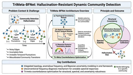
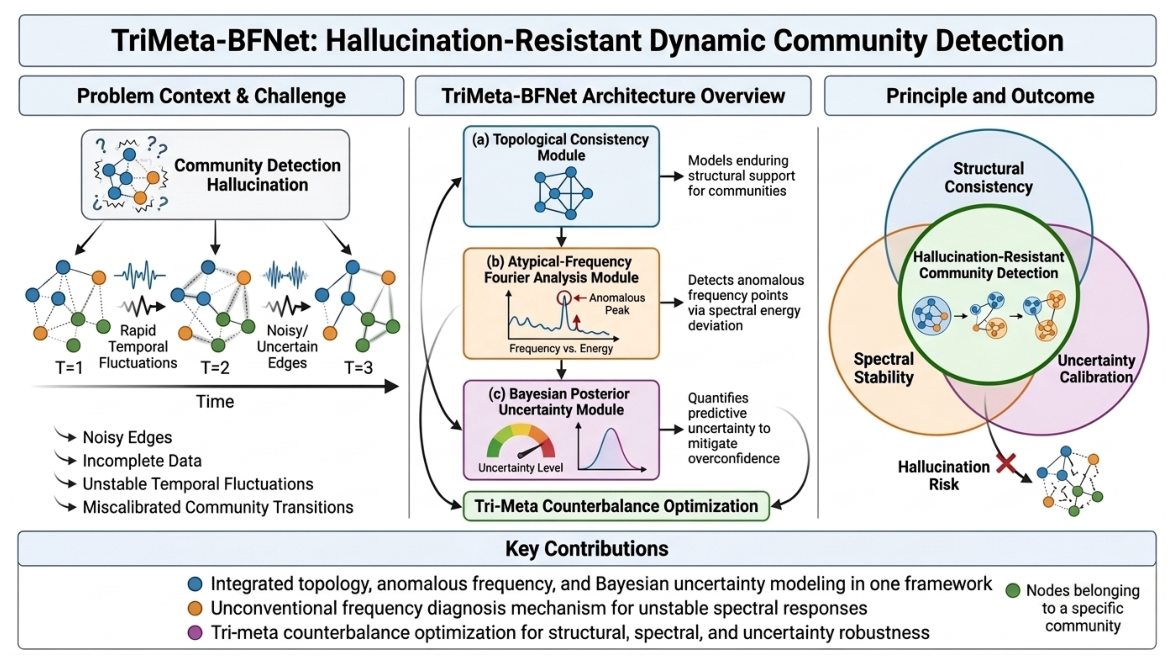
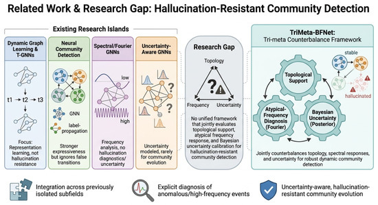
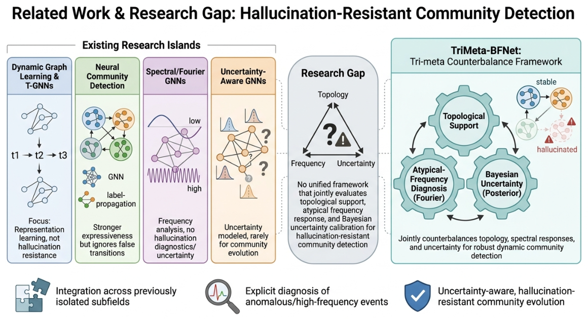
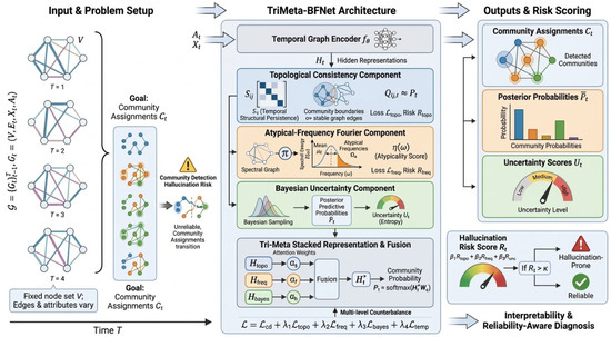
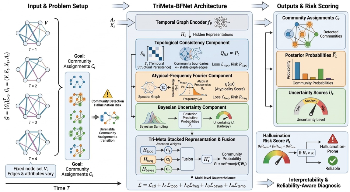
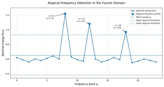
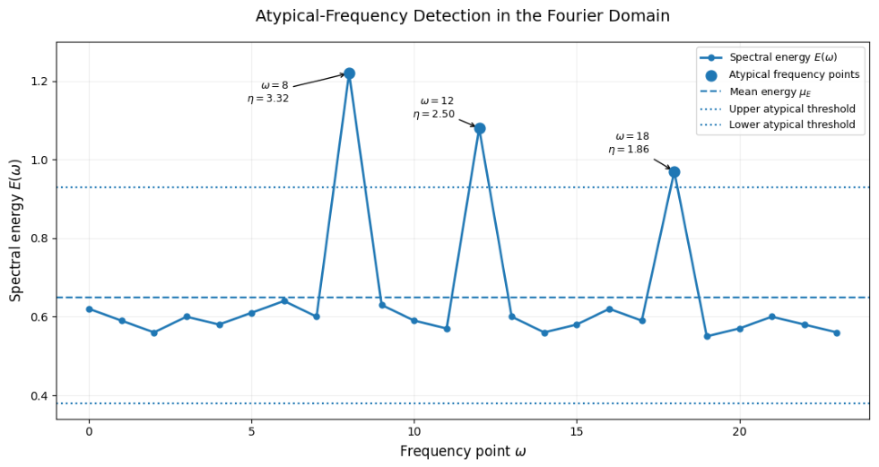
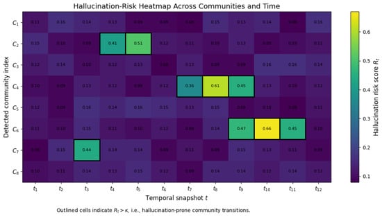
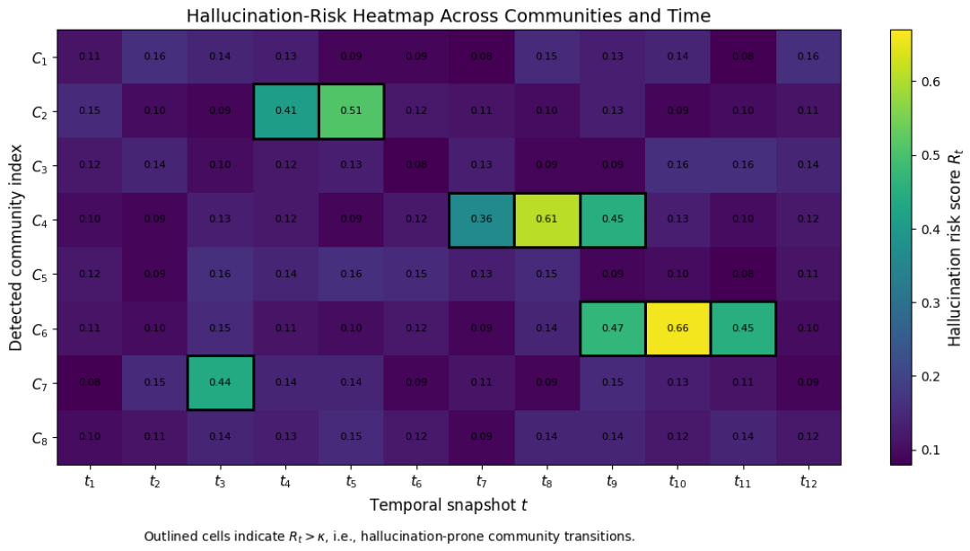
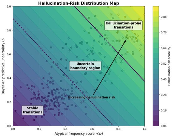
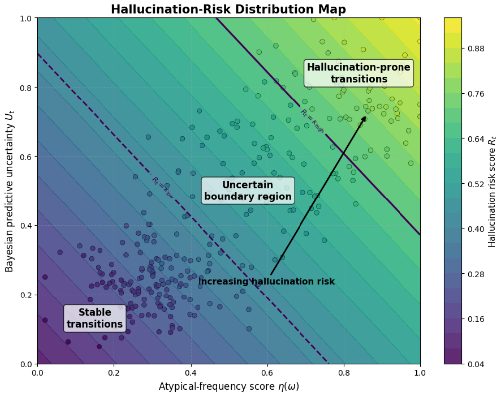
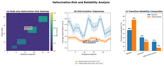
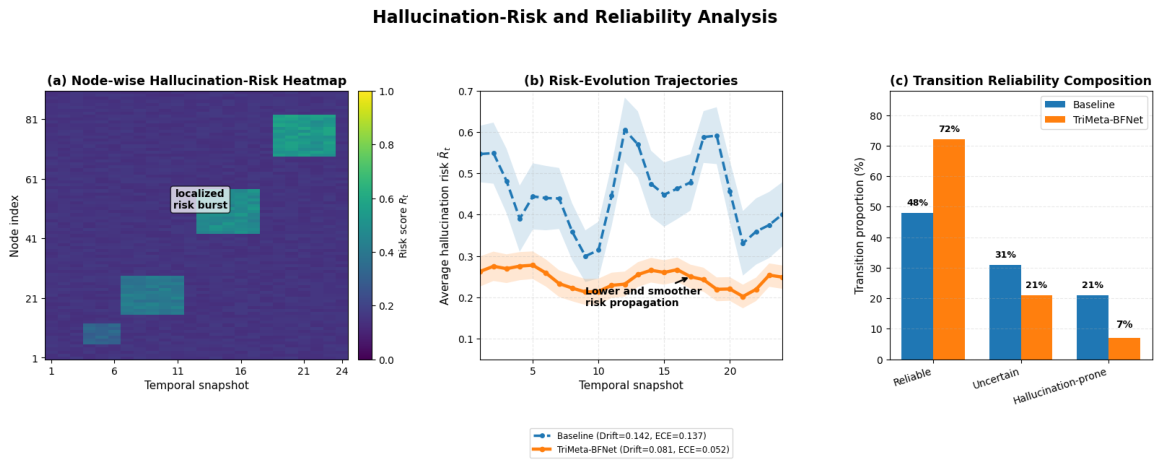
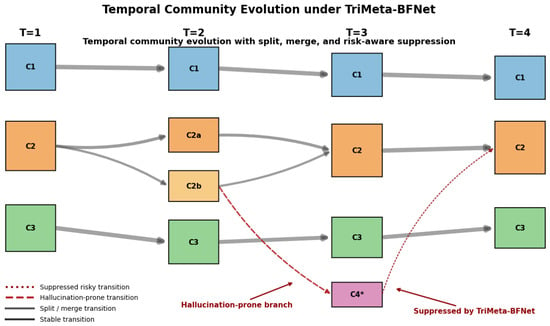
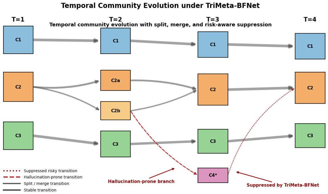
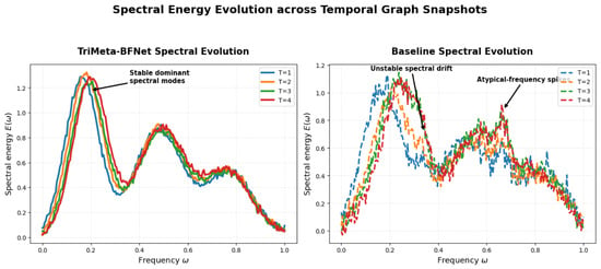
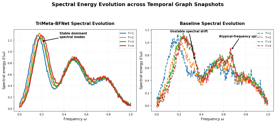
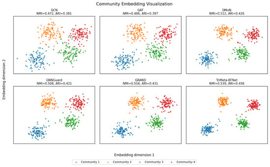
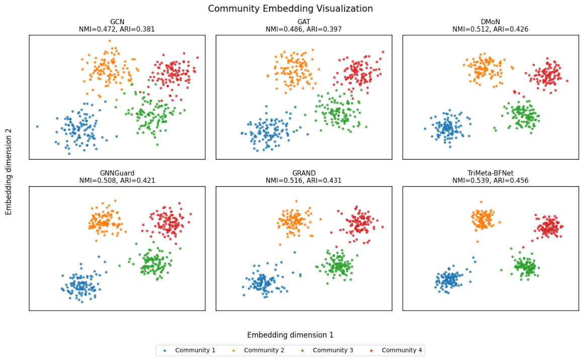
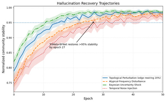
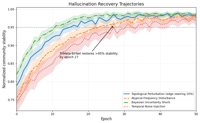
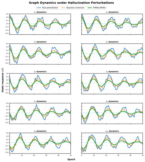
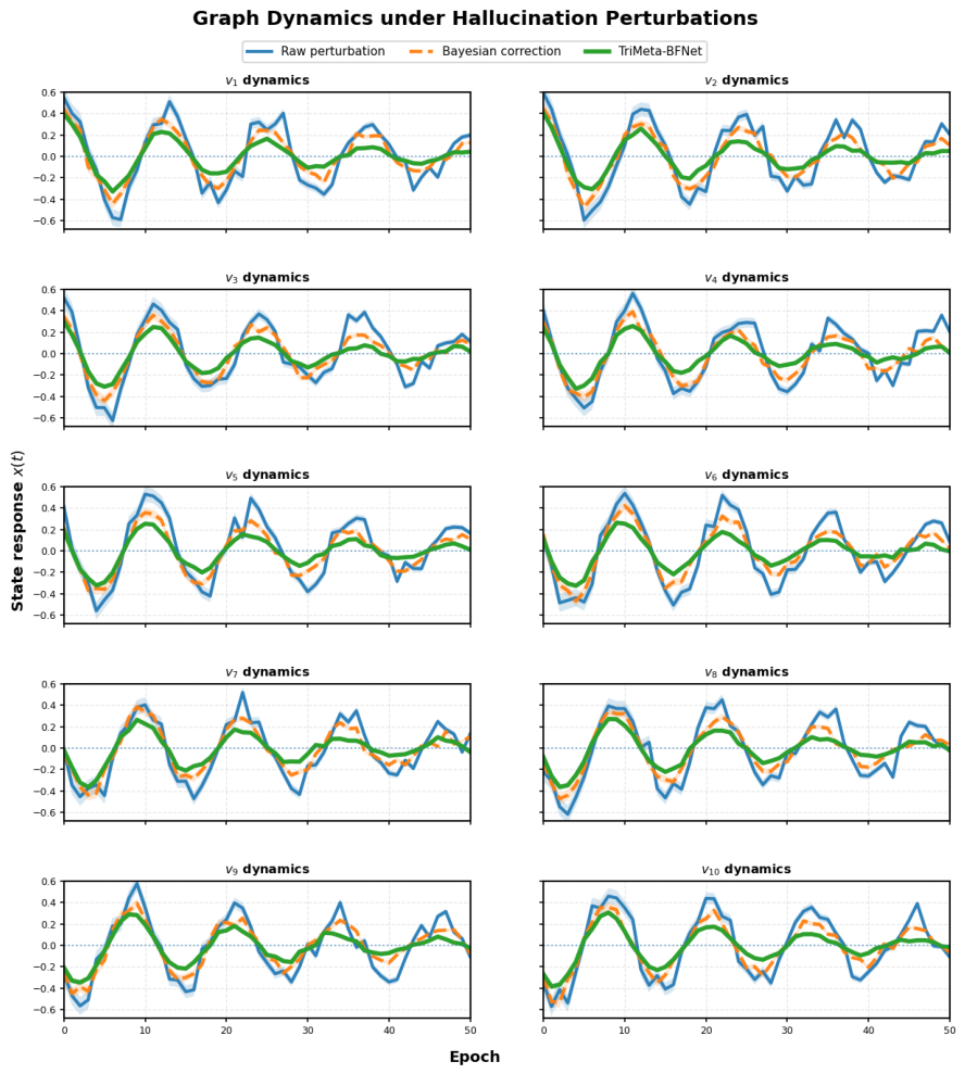
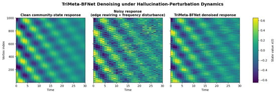
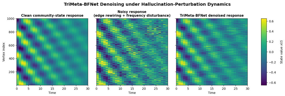
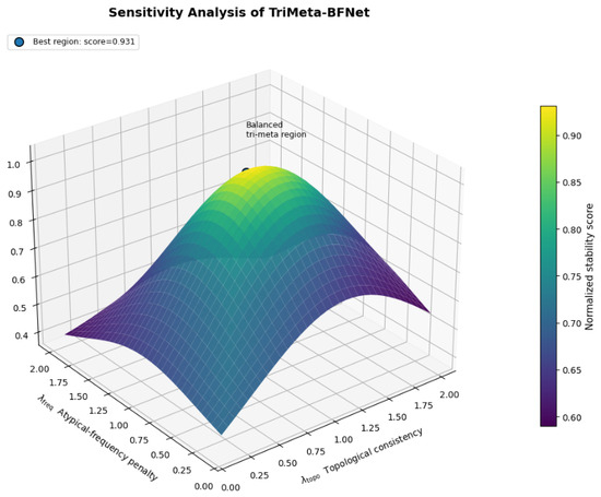
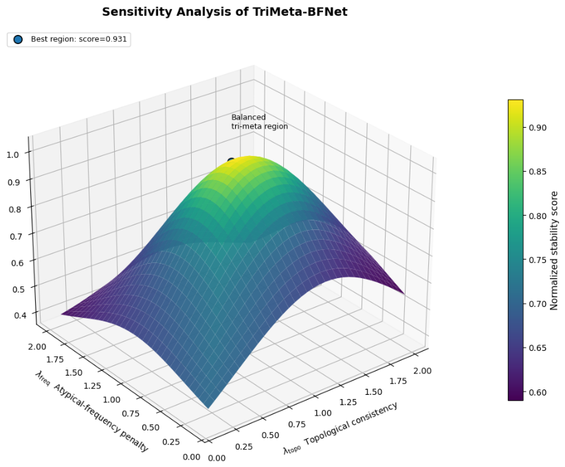

Disclaimer/Publisher’s Note: The statements, opinions and data contained in all publications are solely those of the individual author(s) and contributor(s) and not of MDPI and/or the editor(s). MDPI and/or the editor(s) disclaim responsibility for any injury to people or property resulting from any ideas, methods, instructions or products referred to in the content. |
© 2026 by the authors. Licensee MDPI, Basel, Switzerland. This article is an open access article distributed under the terms and conditions of the Creative Commons Attribution (CC BY) license.