Stochastic Environmental Impacts on Two-Patch Cholera Model: Threshold Analysis and Ergodic Stationary Distribution

Abstract

In-depth analysis of epidemic models, particularly for cholera, is crucial because they serve as significant tools for disease transmission prediction, evaluation of control strategies, and optimization of healthcare resource management. The stochastic models provide increased realism by incorporating environmental uncertainty such as variability in water quality, disparities in access to sanitation, and population mobility. The present work generalizes a deterministic two-patch cholera model to a stochastic framework. We first prove the existence and uniqueness of global solutions, then establish the extinction condition $R_0^{*}<1$ for disease eradication in the long term. A key contribution lies in proving the existence of a unique ergodic stationary distribution when $R_0^{\left(1\right)}>1$ and $R_0^{\left(2\right)}>1$. Furthermore, we derive the stochastic threshold $R_0=\text{max}\{R_0^{\left(1\right)},R_0^{\left(2\right)}\}$, which corresponds to the basic reproduction number ${\mathcal{R}}_0=\text{max}\{{\mathcal{R}}_0^{\left(1\right)},{\mathcal{R}}_0^{\left(2\right)}\}$. Lastly, numerical simulations are employed to confirm theoretical results.

1. Introduction

Mathematical modeling became a fundamental tool for the study of infectious disease dynamics, with numerous studies employing systems of ordinary differential equations [1,2,3,4]. Cholera is a water-borne disease caused by Vibrio cholerae that poses significant epidemiological challenges due to its dual transmission pathway: direct human-to-human transmission and indirect transmission through contaminated water reservoirs. The latter is particularly important because the sources of water are often contaminated by the discharge of patients with the infection. Global burden estimates are 1.3–4.0 million cases and 21,000–143,000 deaths annually [5]. Following Capasso’s milestone 1979 paper [6] presenting a two-dimensional system model of host-pathogen interaction, the following cholera modeling structures have had a much wider scope, including deeper transmission dynamics. For example, by adding the susceptible population to Capasso’s model, Codeço [7] proposed an SIR (susceptible-infected-recovered) model. Afterward, Hartely et al. [8] stretched the SIR formulation raised in [7] by incorporating a state of hyper-infectivity. An overview of single-patch models can be found in the review papers [9,10,11,12,13] and their references. The model explored by Eisenberg et al. [14] incorporates both direct and indirect transmission pathways, as well as water and human movements across patches. The authors treated water movement as migration, which may not accurately reflect real-world scenarios. A patch model excluding human movement is examined in [15]. A periodic transmission rate was incorporated into a cholera epidemic model by Zhou and Cui [16] in 2013. By incorporating migration into cholera dynamics, Njagarah and Nyabadza [17] developed a metapopulation model that describes cholera transmission between two communities connected by migratory movement. A two-patch epidemiological model for cholera with distinct fast and slow transmission rates was formulated by Berge and colleagues [18] in 2017. In 2023, Cheng et al. [19] developed a new network-based cholera model with an explicit demographic structure, incorporating multiple transmission pathways, including both environment-to-human and human-to-human transmission. In their framework, human contacts are represented through a heterogeneous contact network, while interactions between humans and the environment are modeled under a homogeneous-mixing assumption. For a systematic and critical review of the literature on approaches used in cholera disease, readers are referred to [20].

Ordinary differential equations (ODEs) yield a deterministic approach to modeling biological systems, but cannot incorporate the intrinsic randomness of disease dynamics and population interactions. Stochastic differential equations (SDEs) are obtained by incorporating random terms into ODEs so better model the inherent randomness present in biological systems. This capability is especially useful in epidemiology and systems biology, where environmental noise, genetic variation, and random contact patterns play an important role in determining outcomes. SDEs allow us to quantify uncertainty in disease spread, predict key events such as pathogen extinction or emergence, and measure how biological systems respond to stochastic fluctuations. In contrast to deterministic models, SDEs reveal how small random fluctuations affect long-term behavior, thereby providing greater insight into ecosystem stability, infection persistence, and the effectiveness of public health interventions. By incorporating inherent variability, stochastic models provide a more realistic description of complex biological systems and are therefore essential for investigating infectious diseases and population dynamics.

In recent years, numerous studies have employed this stochastic approach to simulate cholera epidemic dynamics, with particular emphasis on the effect of random fluctuations on disease transmission patterns, see, for example, [21,22,23,24,25]. Also, using a stochastic modeling framework, Liu and Jiang [26] analyzed cholera dynamics in the context of imperfect vaccine efficacy. Unlike single-patch models, Liu and colleagues’ [27] stochastic model treated cholera spread through a migration network among groups. Song et al. [28] develop a stochastic compartmental cholera model with multiple water-borne transmission pathways, offering a more realistic representation of the disease dynamics compared with earlier formulations. Zhou, Shi and Wei [29] introduced a stochastic model of cholera transmission with a recovery rate that depends on saturation. The stochastic cholera model introduced by Zhu et al. [30] incorporated both Brownian motion and Lévy jump noise simultaneously to more accurately capture the variability of epidemics in real-world scenarios.

In this article, we formulate a stochastic version of the cholera transmission model (1) to investigate disease dynamics with particular attention to long-term behavior upon human population movement between two linked patches. Using stochastic analysis techniques, we prove that the stochastic system (2) possesses a unique global positive solution for any time $t\ge 0$. Our analysis demonstrates an intrinsic relationship between the deterministic basic reproduction number $({\mathcal{R}}_0=\text{max}\{{\mathcal{R}}_0^{\left(1\right)},{\mathcal{R}}_0^{\left(2\right)}\})$ and its stochastic counterpart $(R_0=\text{max}\{R_0^{\left(1\right)},R_0^{\left(2\right)}\})$ in epidemic modeling. We derive necessary and sufficient conditions for almost sure extinction of solutions of system (2), and verify that if $R_0^{\left(1\right)}>1$ and $R_0^{\left(2\right)}>1$, then the stochastic model (2) admits a unique ergodic stationary distribution.

This study advances the stochastic modeling of cholera by formulating and analyzing a two-patch model in which environmental variability is incorporated as multiplicative noise into the equations for all human subpopulations (susceptible, infected, and recovered) and the environmental pathogen concentration. This approach enhances mathematical realism by accounting for uncertainty across all transmission pathways. Moreover, we rigorously establish analytical conditions for both disease extinction and the existence and uniqueness of an ergodic stationary distribution. These results link the system’s steady-state behavior to patch-specific thresholds and clarify how noise influences disease persistence in coupled systems.

In contrast to previous stochastic cholera models, the present work incorporates a two-community structure together with a fast-slow transmission mechanism within a stochastic multi-patch framework. While multi-patch SDE models such as those in Song et al. [28] study migration and noise effects, they do not account for the inherent timescale separation between rapid person-to-person transmission and slow environmental pathways. This epidemiologically important and mathematically nontrivial feature requires the construction of a new Lyapunov functional that can handle coupled fast-slow dynamics across communities. Our analysis further yields a novel threshold condition of the form $R_0=\text{max}\{R_0^{\left(1\right)},R_0^{\left(2\right)}\}$, along with stationary distributions and transient behaviors that existing stochastic cholera models do not capture. By integrating multi-patch structure, time-scale separation, and stochasticity, this study advances the theoretical understanding of cholera persistence under realistic transmission heterogeneities.

In the deterministic model, the reproductive number ${\mathcal{R}}_0$ is a threshold value that determines whether the disease invades the population. In the stochastic model, in contrast, the process is governed by a different quantity, denoted by $R_0$. Unlike its deterministic counterpart, $R_0$ does not serve as an invasion threshold; instead, it affects the probability of disease extinction and the existence of a stationary distribution. Specifically, even if ${\mathcal{R}}_0>1$, stochastic noise can still cause disease extinction with positive probability. Moreover, $R_0$ determines when the system is ergodic and converges to a unique endemic stationary distribution.

The paper is organized as follows. The stochastic version of the cholera model is formulated in Section 2. The global existence and positivity of the solution system (2) are provided in Section 3. The next section derives sufficient conditions for almost sure extinction of the disease in the stochastic cholera model (2). We establish conditions for the existence of the ergodic stationary distribution in Section 5. To substantiate our theoretical analysis, we conduct extensive numerical simulations in Section 6. Section 7 concludes this paper.

2. Model Formulation

Berge, Bowong and Lubuma [18] formulated an ODE-based model to analyze cholera epidemiology in their 2017 work. This deterministic model is built to investigate how human mobility in two connected patches influences the dynamics of the disease. The model formulation is given by:

$$\left\{\begin{array}{cc}\hfill & {\displaystyle \frac{\mathrm{d}{\mathfrak{X}}_{t,1}^{\mathbb{S}}}{\mathrm{d}t}}={\mathcal{A}}_1-{\lambda }_1{\mathfrak{X}}_{t,1}^{\mathbb{S}}{\mathfrak{X}}_{t,1}^{\mathbb{W}}-{\beta }_1{\mathfrak{X}}_{t,1}^{\mathbb{S}}{\mathcal{I}}_{t,1}-({\mu }_1+a_1){\mathfrak{X}}_{t,1}^{\mathbb{S}}+a_2{\mathfrak{X}}_{t,2}^{\mathbb{S}},\hfill \\ \hfill & {\displaystyle \frac{\mathrm{d}{\mathfrak{X}}_{t,2}^{\mathbb{I}}}{\mathrm{d}t}}={\lambda }_1{\mathfrak{X}}_{t,1}^{\mathbb{S}}{\mathfrak{X}}_{t,1}^{\mathbb{W}}+{\beta }_1{\mathfrak{X}}_{t,1}^{\mathbb{S}}{\mathfrak{X}}_{t,1}^{\mathbb{I}}-({\mu }_1+{\delta }_1+{\gamma }_1){\mathfrak{X}}_{t,1}^{\mathbb{I}},\hfill \\ \hfill & {\displaystyle \frac{\mathrm{d}{\mathfrak{X}}_{t,2}^{\mathbb{S}}}{\mathrm{d}t}}={\mathcal{A}}_2-{\lambda }_2{\mathfrak{X}}_{t,2}^{\mathbb{S}}{\mathfrak{X}}_{t,2}^{\mathbb{W}}-{\beta }_2{\mathfrak{X}}_{t,2}^{\mathbb{S}}{\mathfrak{X}}_{t,2}^{\mathbb{I}}-({\mu }_2+a_2){\mathfrak{X}}_{t,2}^{\mathbb{S}}+a_1{\mathfrak{X}}_{t,1}^{\mathbb{S}},\hfill \\ \hfill & {\displaystyle \frac{\mathrm{d}{\mathfrak{X}}_{t,2}^{\mathbb{I}}}{\mathrm{d}t}}={\lambda }_2{\mathfrak{X}}_{t,2}^{\mathbb{S}}{\mathfrak{X}}_{t,2}^{\mathbb{W}}+{\beta }_2{\mathfrak{X}}_{t,2}^{\mathbb{S}}{\mathfrak{X}}_{t,2}^{\mathbb{I}}-({\mu }_2+{\delta }_2+{\gamma }_2){\mathfrak{X}}_{t,2}^{\mathbb{I}},\hfill \\ \hfill & {\displaystyle \frac{\mathrm{d}{\mathfrak{X}}_{t,1}^{\mathbb{W}}}{\mathrm{d}t}}={\epsilon }_1\left({\mathfrak{X}}_{t,1}^{\mathbb{I}}-{\mathfrak{X}}_{t,1}^{\mathbb{W}}\right),\hfill \\ \hfill & {\displaystyle \frac{\mathrm{d}{\mathfrak{X}}_{t,2}^{\mathbb{W}}}{\mathrm{d}t}}={\epsilon }_2\left({\mathfrak{X}}_{t,2}^{\mathbb{I}}-{\mathfrak{X}}_{t,2}^{\mathbb{W}}\right).\hfill \end{array}\right.$$

(1)

In model (1), ${\mathfrak{X}}_{t,k}^{\mathbb{S}}$ and ${\mathfrak{X}}_{t,k}^{\mathbb{I}}$ are used to describe the population sizes of individuals in patch $k(k=1,2)$ who are susceptible to infection and infected from infection at time t, respectively. The concentration of Vibrio cholerae in the aquatic reservoir in patch k is represented by ${\mathfrak{X}}_{t,k}^{\mathbb{B}}$. A constant recruitment rate ${\mathcal{A}}_k$ is assumed for the susceptible class in patch k, accounting for births, immigration, or the loss of temporary immunity. Susceptible individuals in patch k can be infected by Vibrio cholerae through two different transmission modes: human-to-human contact (fast transmission) at a rate ${\beta }_k$ and contact with contaminated water (slow transmission) at a rate ${\lambda }_{b,k}$. Infected individuals shed Vibrio cholerae into the water reservoir at a rate ${\alpha }_k$ and thereby contaminate it. The decay rate ${\epsilon }_k$ is a net decay rate for Vibrio cholerae in the aquatic reservoir and is assumed to be dominated by decay over birth and reproduction. The recovery of infected individuals is governed by the rate ${\gamma }_k$, whereas natural mortality affects all the compartments of the human populations uniformly at a rate ${\mu }_k$. The infected individuals also suffer a disease-related mortality at a rate ${\delta }_k$. In view of the severity of the disease, the movement of individuals between the patches within the susceptible and infected classes is restricted. The per capita rate of outward migration of the susceptible individuals from the k-th patch is represented by $a_k$. To simplify the notation, we define the composite parameter as ${\lambda }_k={\displaystyle \frac{{\alpha }_k{\lambda }_{b,k}}{{\epsilon }_k}}$ and the scaled pathogen concentration as ${\mathfrak{X}}_{t,k}^{\mathbb{W}}={\displaystyle \frac{{\epsilon }_k}{{\alpha }_k}}{\mathfrak{X}}_{t,k}^{\mathbb{B}}$, $k=1,2$. The summary of all the state variables and parameters is given in Table 1.

Table 1. Variables and parameters with units for the system (1).

Symbols	Definitions	Units
${\mathfrak{X}}_k^{\mathbb{S}}$	Susceptible individuals	individual
${\mathfrak{X}}_k^{\mathbb{I}}$	Infected individuals	individual
${\mathfrak{X}}_k^{\mathbb{B}}$	Pathogen concentration in water	individual
${\lambda }_{b,k}$	Water-to-human per capita contact rate	cell−1mL−1day−1
${\beta }_k$	Human-to-human per capita contact rate	individual−1day−1
${\mu }_k$	Natural death rate of individuals	day−1
${\gamma }_k$	Recovered rate of individuals	day−1
${\delta }_k$	Disease death rate of individuals	day−1
${\alpha }_k$	Pathogen shedding rate (human–water contact rate)	cell mL−1day−1individual−1
${\epsilon }_k$	Net pathogen decay rate	day−1
${\mathcal{A}}_k$	Recruitment of susceptible individuals	individual day−1
$a_k$	Migration rate of susceptible individuals to patch k	day−1

Let ${\mathfrak{X}}_t^{\mathbb{N}}={\mathfrak{X}}_{t,1}^{\mathbb{S}}+{\mathfrak{X}}_{t,1}^{\mathbb{I}}+{\mathfrak{X}}_{t,2}^{\mathbb{S}}+{\mathfrak{X}}_{t,2}^{\mathbb{I}}$ and ${\mathfrak{X}}_t^{\mathbb{W}}={\mathfrak{X}}_{t,1}^{\mathbb{W}}+{\mathfrak{X}}_{t,2}^{\mathbb{W}}$. Then the set

$$\Sigma =\left\{\left({\mathfrak{X}}_{t,1}^{\mathbb{S}},{\mathfrak{X}}_{t,1}^{\mathbb{I}},{\mathfrak{X}}_{t,2}^{\mathbb{S}},{\mathfrak{X}}_{t,2}^{\mathbb{I}},{\mathfrak{X}}_{t,1}^{\mathbb{W}},{\mathfrak{X}}_{t,2}^{\mathbb{W}}\right)\in {\mathbb{R}}_{+}^6/{\mathfrak{X}}_t^{\mathbb{N}}\le {\displaystyle \frac{\mathcal{A}}{{\mu }_0}},{\mathfrak{X}}_t^{\mathbb{W}}\le {\displaystyle \frac{\overline{\epsilon }\mathcal{A}}{\underline{\epsilon }{\mu }_0}}\right\},$$

with $\mathcal{A}={\mathcal{A}}_1+{\mathcal{A}}_2$, ${\mu }_0=\text{min}\{{\mu }_1,{\mu }_2\}$, $\overline{\epsilon }=\text{max}\{{\epsilon }_1,{\epsilon }_2\}$ and $\underline{\epsilon }=\text{min}\{{\epsilon }_1,{\epsilon }_2\}$, is positively invariant for system (1), ensuring biological realism. The epidemiological threshold of system (1) by the basic reproduction number ${\mathcal{R}}_0=\text{max}\left\{{\mathcal{R}}_0^{\left(1\right)},{\mathcal{R}}_0^{\left(2\right)}\right\}$, where

$${\mathcal{R}}_0^{\left(1\right)}={\displaystyle \frac{({\lambda }_1+{\beta }_1)({\mathcal{A}}_1({\mu }_2+a_2)+{\mathcal{A}}_2{a}_2)}{({\mu }_1+{\delta }_1+{\gamma }_1)({\mu }_1{\mu }_2+{\mu }_1{a}_2+{\mu }_2{a}_1)}},{\mathcal{R}}_0^{\left(2\right)}={\displaystyle \frac{({\lambda }_2+{\beta }_2)({\mathcal{A}}_2({\mu }_1+a_1)+{\mathcal{A}}_1{a}_1)}{({\mu }_2+{\delta }_2+{\gamma }_2)({\mu }_1{\mu }_2+{\mu }_1{a}_2+{\mu }_2{a}_1)}}.$$

System (1) also possesses four distinct equilibrium points (i) the disease-free equilibrium $E_0=({\mathfrak{S}}_1^0,0,0,{\mathfrak{S}}_2^0,0,0)$ with

$${\mathfrak{S}}_1^0={\displaystyle \frac{{\mathcal{A}}_1({\mu }_2+a_2)+{\mathcal{A}}_2{a}_2}{{\mu }_1{\mu }_2+{\mu }_1{a}_2+{\mu }_2{a}_1}},{\mathfrak{S}}_2^0={\displaystyle \frac{{\mathcal{A}}_2({\mu }_1+a_1)+{\mathcal{A}}_1{a}_1}{{\mu }_1{\mu }_2+{\mu }_1{a}_2+{\mu }_2{a}_1}},$$

and (ii) three endemic equilibria $E^{*}=({\mathfrak{S}}_1^{*},{\mathfrak{I}}_1^{*},{\mathfrak{W}}_1^{*},{\mathfrak{S}}_2^{*},0,0)$ with

$$\begin{array}{cc}\hfill {\mathfrak{S}}_1^{*}& ={\displaystyle \frac{{\mu }_1+{\delta }_1+{\gamma }_1}{{\lambda }_1+{\beta }_1}},{\mathfrak{I}}_1^{*}={\mathfrak{W}}_1^{*}={\displaystyle \frac{({\mathcal{A}}_1({\mu }_2+a_2)+{\mathcal{A}}_2{a}_2)({\mathcal{R}}_0^{\left(1\right)}-1)}{({\mu }_1+{\delta }_1+{\gamma }_1)({\mu }_2+a_2){\mathcal{R}}_0^{\left(1\right)}}},\hfill \\ \hfill {\mathfrak{S}}_2^{*}& ={\displaystyle \frac{{\mathcal{A}}_1({\lambda }_1+{\beta }_1)+a_1({\mu }_1+{\delta }_1+{\gamma }_1)}{({\lambda }_1+{\beta }_1)({\mu }_2+a_2)}},\hfill \end{array}$$

$E^{**}=({\mathfrak{S}}_1^{**},0,0,{\mathfrak{S}}_2^{**},{\mathfrak{I}}_1^{**},{\mathfrak{W}}_1^{**})$ with

$$\begin{array}{cc}\hfill {\mathfrak{S}}_1^{**}& ={\displaystyle \frac{{\mathcal{A}}_1({\lambda }_2+{\beta }_2)+a_2({\mu }_2+{\delta }_2+{\gamma }_2)}{({\lambda }_2+{\beta }_2)({\mu }_1+a_1)}},{\mathfrak{S}}_2^{*}={\displaystyle \frac{{\mu }_2+{\delta }_2+{\gamma }_2}{{\lambda }_2+{\beta }_2}},\hfill \\ \hfill {\mathfrak{I}}_2^{*}& ={\mathfrak{W}}_2^{*}={\displaystyle \frac{({\mathcal{A}}_2({\mu }_1+a_1)+{\mathcal{A}}_1{a}_1)({\mathcal{R}}_0^{\left(2\right)}-1)}{({\mu }_2+{\delta }_2+{\gamma }_2)({\mu }_1+a_1){\mathcal{R}}_0^{\left(2\right)}}},\hfill \end{array}$$

and $\overline{E}=({\mathfrak{S}}_1^{*},{\overline{\mathfrak{I}}}_1,{\overline{\mathfrak{W}}}_1,{\mathfrak{S}}_2^{**},{\overline{\mathfrak{I}}}_2,{\overline{\mathfrak{W}}}_2)$ with

$${\overline{\mathfrak{I}}}_1={\overline{\mathfrak{W}}}_1={\displaystyle \frac{({\mu }_1+a_1)}{({\lambda }_1+{\beta }_1)}}({\mathfrak{T}}_1-1),{\overline{\mathfrak{I}}}_2={\overline{\mathfrak{W}}}_2={\displaystyle \frac{({\mu }_2+a_2)}{({\lambda }_2+{\beta }_2)}}({\mathfrak{T}}_2-1),$$

where

$${\mathfrak{T}}_1={\displaystyle \frac{({\lambda }_1+{\beta }_1)}{({\mu }_1+{\delta }_1+{\gamma }_1)}}{\mathfrak{S}}_1^{**},{\mathfrak{T}}_2={\displaystyle \frac{({\lambda }_2+{\beta }_2)}{({\mu }_2+{\delta }_2+{\gamma }_2)}}{\mathfrak{S}}_2^{*}.$$

As shown in [18], the analysis of stability system (1) reveals the following:

• The disease-free equilibrium $E_0$ is locally asymptotically stable in $\Sigma$ when ${\mathcal{R}}_0<1$ and unstable when ${\mathcal{R}}_0>1$.
• The global asymptotically stability of the disease-free equilibrium $E_0$ is guaranteed whenever both threshold parameters meet the conditions ${\mathcal{R}}_0^{\left(1\right)}\le 1$ and ${\mathcal{R}}_0^{\left(2\right)}\le 1$.
• Patch 1 can sustain a disease-free equilibrium $E^{*}$ if the basic reproduction number fulfills ${\mathcal{R}}_0^{\left(1\right)}>1$ and ${\mathcal{R}}_0^{\left(2\right)}\le 1$. On the other hand, disease-free equilibrium $E^{**}$ occurs in patch 2 when ${\mathcal{R}}_0^{\left(1\right)}\le 1$ and ${\mathcal{R}}_0^{\left(2\right)}>1$.
• Whenever both conditions ${\mathfrak{T}}_1>1$ and ${\mathfrak{T}}_2>1$ are satisfied, the internal equilibrium $\overline{E}$ holds.
• Let ${\mathcal{R}}_0^{\left(1\right)}>1$ and ${\mathcal{R}}_0^{\left(2\right)}\le 1$. Under these assumptions, the boundary equilibrium $E^{*}$ is locally asymptotically stable when ${\mathfrak{T}}_2\le 1$ and unstable when ${\mathfrak{T}}_2>1$.
• In the domain $\Sigma$, aside from the manifold $\{{\mathfrak{X}}_{t,1}^{\mathbb{I}}={\mathfrak{X}}_{t,1}^{\mathbb{W}}=0\}$, the boundary equilibrium $E^{*}$ is globally asymptotically stable under conditions that ${\mathcal{R}}_0^{\left(1\right)}>1$, ${\mathcal{R}}_0^{\left(2\right)}\le 1$ and ${\mathfrak{T}}_2\le 1$.
• Let ${\mathcal{R}}_0^{\left(1\right)}\le 1$ and ${\mathcal{R}}_0^{\left(2\right)}>1$. Then, in these conditions, system (1) has locally asymptotically stable boundary equilibrium $E^{**}$ if ${\mathfrak{T}}_1\le 1$ and unstable if ${\mathfrak{T}}_1>1$.
• Assuming ${\mathcal{R}}_0^{\left(1\right)}\le 1$, ${\mathcal{R}}_0^{\left(2\right)}>1$ and ${\mathfrak{T}}_1\le 1$, boundary equilibrium $E^{**}$ is globally asymptotically stable in the domain $\Sigma$, except for the manifold $\{{\mathfrak{X}}_{t,2}^{\mathbb{I}}={\mathfrak{X}}_{t,2}^{\mathbb{W}}=0\}$.
• Condition ${\mathfrak{T}}_1>1$ and ${\mathfrak{T}}_2>1$ is sufficient to ensure the local asymptotic stability of endemic equilibrium $\overline{E}$.
• The interior endemic equilibrium $\overline{E}$ is globally asymptotically stable in the interior of $\Sigma$ if ${\mathfrak{T}}_1>1$, ${\mathfrak{T}}_2>1$ and if the parameters obey the constraints ${\mathcal{A}}_1-{\lambda }_1{\mathfrak{S}}_1^{*}{\overline{\mathfrak{I}}}_1\ge 0$ and ${\mathcal{A}}_2-{\lambda }_2{\mathfrak{S}}_2^{**}{\overline{\mathfrak{I}}}_2\ge 0$.

The deterministic version in system (1) cannot capture key sources of environmental variability relevant to cholera transmission, such as fluctuations in water contamination, sanitation quality, nutritional factors, and occupational exposure. To address this limitation, we derive a stochastic counterpart by introducing multiplicative noise terms that represent population-level environmental perturbations. We incorporate six independent Wiener processes ${\mathcal{B}}_{t,i}$ with noise intensities ${\sigma }_i>0,i=1,\dots ,6$, each satisfying the standard properties of a zero-mean Gaussian process with stationary independent increments. These stochastic terms represent the combined effect of random environmental disturbances acting on all population compartments. The resulting stochastic differential equations provide a more biologically realistic model that can simulate outbreak patterns under environmental fluctuations while preserving the core transmission structure of system (1). Under these assumptions, the stochastic cholera model is given by

$$\left\{\begin{array}{cc}\hfill & \mathrm{d}{\mathfrak{X}}_{t,1}^{\mathbb{S}}=\left({\mathcal{A}}_1-{\lambda }_1{\mathfrak{X}}_{t,1}^{\mathbb{S}}{\mathfrak{X}}_{t,1}^{\mathbb{W}}-{\beta }_1{\mathfrak{X}}_{t,1}^{\mathbb{S}}{\mathfrak{X}}_{t,1}^{\mathbb{I}}-({\mu }_1+a_1){\mathfrak{X}}_{t,1}^{\mathbb{S}}+a_2{\mathfrak{X}}_{t,2}^{\mathbb{S}}\right)\mathrm{d}t+{\sigma }_1{\mathfrak{X}}_{t,1}^{\mathbb{S}}\mathrm{d}{\mathcal{B}}_{t,1},\hfill \\ \hfill & \mathrm{d}{\mathfrak{X}}_{t,1}^{\mathbb{I}}=\left({\lambda }_1{\mathfrak{X}}_{t,1}^{\mathbb{S}}{\mathfrak{X}}_{t,1}^{\mathbb{W}}+{\beta }_1{\mathfrak{X}}_{t,1}^{\mathbb{S}}{\mathfrak{X}}_{t,1}^{\mathbb{I}}-({\mu }_1+{\delta }_1+{\gamma }_1){\mathfrak{X}}_{t,1}^{\mathbb{I}}\right)\mathrm{d}t+{\sigma }_2{\mathfrak{X}}_{t,1}^{\mathbb{I}}\mathrm{d}{\mathcal{B}}_{t,2},\hfill \\ \hfill & \mathrm{d}{\mathfrak{X}}_{t,2}^{\mathbb{S}}=\left({\mathcal{A}}_2-{\lambda }_2{\mathfrak{X}}_{t,2}^{\mathbb{S}}{\mathfrak{X}}_{t,2}^{\mathbb{W}}-{\beta }_2{\mathfrak{X}}_{t,2}^{\mathbb{S}}{\mathfrak{X}}_{t,2}^{\mathbb{I}}-({\mu }_2+a_2){\mathfrak{X}}_{t,2}^{\mathbb{S}}+a_1{\mathfrak{X}}_{t,1}^{\mathbb{S}}\right)\mathrm{d}t+{\sigma }_3{\mathfrak{X}}_{t,2}^{\mathbb{S}}\mathrm{d}{\mathcal{B}}_{t,3},\hfill \\ \hfill & \mathrm{d}{\mathfrak{X}}_{t,2}^{\mathbb{I}}=\left({\lambda }_2{\mathfrak{X}}_{t,2}^{\mathbb{S}}{\mathfrak{X}}_{t,2}^{\mathbb{W}}+{\beta }_2{\mathfrak{X}}_{t,2}^{\mathbb{S}}{\mathfrak{X}}_{t,2}^{\mathbb{I}}-({\mu }_2+{\delta }_2+{\gamma }_2){\mathfrak{X}}_{t,2}^{\mathbb{I}}\right)\mathrm{d}t+{\sigma }_4{\mathfrak{X}}_{t,2}^{\mathbb{I}}\mathrm{d}{\mathcal{B}}_{t,4},\hfill \\ \hfill & \mathrm{d}{\mathfrak{X}}_{t,1}^{\mathbb{W}}={\epsilon }_1\left({\mathfrak{X}}_{t,1}^{\mathbb{I}}-{\mathfrak{X}}_{t,1}^{\mathbb{W}}\right)\mathrm{d}t+{\sigma }_5{\mathfrak{X}}_{t,1}^{\mathbb{W}}\mathrm{d}{\mathcal{B}}_{t,5},\hfill \\ \hfill & \mathrm{d}{\mathfrak{X}}_{t,2}^{\mathbb{W}}={\epsilon }_2\left({\mathfrak{X}}_{t,2}^{\mathbb{I}}-{\mathfrak{X}}_{t,2}^{\mathbb{W}}\right)\mathrm{d}t+{\sigma }_6{\mathfrak{X}}_{t,2}^{\mathbb{W}}\mathrm{d}{\mathcal{B}}_{t,6}.\hfill \end{array}\right.$$

(2)

The shift from a deterministic to a stochastic framework is justified by the need to incorporate key sources of environmental and demographic variability inherent to cholera transmission dynamics. This stochastic extension is achieved by introducing independent Wiener processes multiplicatively to capture random fluctuations in each compartment. The epidemiological rationale for this noise structure is linked to biological and ecological uncertainties. The pathogen noise models stochastic fluctuations in Vibrio cholerae concentration in the aquatic reservoir, driven by environmental variations such as temperature, salinity, nutrient levels, and copepod presence [31,32]. Likewise, the Wiener processes coupled to transmission rates reflect randomness in sanitation practices, hygiene compliance, and contact patterns [33,34]. Demographic stochasticity in population mobility is captured through noise in migration rates, accounting for unpredictable movement influenced by daily routines, economic activities, or seasonal travel [35,36]. This formulation posits that environmental noise primarily affects the pathogen reservoir and transmission pathways, while demographic noise influences mobility and vital dynamics. Incorporating these multiplicative noise terms yields a model that transcends mean-field approximations and provides a realistic representation of cholera dynamics in heterogeneous environments. This stochastic framework is theoretical and establishes general principles governing how noise shapes extinction and persistence, and it forms a foundation for future applied studies in which noise intensities may be informed by empirical data.

The stochastic modeling framework developed here is a theoretical and methodological contribution to infectious disease dynamics. It aims to extend deterministic approaches into a comprehensive stochastic setting and derive general analytical results on long-term behavior. Consequently, the model provides a foundational structure for future applied work, in which parameter estimates from real-world data can support quantitative risk prediction and evaluation of control strategies in heterogeneous environments.

The stochastic structure of model (2) was chosen based on the following considerations. Noise terms are introduced as independent, multiplicative Wiener processes applied to the state equations. Assuming independence across patches and compartments is a conservative simplification that isolates patch-specific stochastic effects and avoids imposing cross-correlations without data. The multiplicative form reflects the empirical observation that the amplitude of fluctuations scales with the magnitude of state variables and ensures non-negativity of the states. Applying noise directly to the state equations captures the broader impact of environmental variability, which can simultaneously affect transmission, recovery, and pathogen decay. Although alternative structures, such as correlated noise or parameter perturbation, are possible, the adopted formulation balances biological realism, mathematical tractability, and the objectives of this study.

3. Existence and Uniqueness of the Global Positive Solution

To prove the existence and uniqueness of a strong solution for system (2), we first observe that the drift and diffusion coefficients are locally Lipschitz continuous and satisfy linear growth conditions. These conditions are standard and ensure that for any initial condition, there exists a unique maximal local solution. Under additional regularity, the solution is positive and does not explode in finite time.

Using stochastic analysis techniques, we first establish that system (2) possesses a unique global solution that remains in the epidemiologically meaningful state space ${\mathbb{R}}_{+}^6$ almost surely (a.s.). Here, by “almost surely” we mean that the stated property holds with probability one, which is the standard notation of certainty in probabilistic settings. The rigorous mathematical assertion is presented in the next theorem:

Theorem 1.

For any initial value $\left({\mathfrak{X}}_{0,1}^{\mathbb{S}},{\mathfrak{X}}_{0,1}^{\mathbb{I}},{\mathfrak{X}}_{0,2}^{\mathbb{S}},{\mathfrak{X}}_{0,2}^{\mathbb{I}},{\mathfrak{X}}_{0,1}^{\mathbb{W}},{\mathfrak{X}}_{0,2}^{\mathbb{W}}\right)\in {\mathbb{R}}_{+}^6$, there is a unique solution $\left({\mathfrak{X}}_{t,1}^{\mathbb{S}},{\mathfrak{X}}_{t,1}^{\mathbb{I}},{\mathfrak{X}}_{t,2}^{\mathbb{S}},{\mathfrak{X}}_{t,2}^{\mathbb{I}},{\mathfrak{X}}_{t,1}^{\mathbb{W}},{\mathfrak{X}}_{t,2}^{\mathbb{W}}\right)$ of system (2) on $t\ge 0$ and the solution will remain in ${\mathbb{R}}_{+}^6$ with probability one, namely, $\left({\mathfrak{X}}_{t,1}^{\mathbb{S}},{\mathfrak{X}}_{t,1}^{\mathbb{I}},{\mathfrak{X}}_{t,2}^{\mathbb{S}},{\mathfrak{X}}_{t,2}^{\mathbb{I}},{\mathfrak{X}}_{t,1}^{\mathbb{W}},{\mathfrak{X}}_{t,2}^{\mathbb{W}}\right)\in {\mathbb{R}}_{+}^6$ for all $t\ge 0$,a.s.

Proof. 

Obviously, the coefficients of system (2) satisfy the local Lipschitz continuity conditions. Therefore, it can be achieved that there exists a unique local solution $\left({\mathfrak{X}}_{0,1}^{\mathbb{S}},{\mathfrak{X}}_{0,1}^{\mathbb{I}},{\mathfrak{X}}_{0,2}^{\mathbb{S}},{\mathfrak{X}}_{0,2}^{\mathbb{I}},{\mathfrak{X}}_{0,1}^{\mathbb{W}},{\mathfrak{X}}_{0,2}^{\mathbb{W}}\right)\in {\mathbb{R}}_{+}^6$ on $t\in [0,{\tau }_e)$ with any initial value $\left({\mathfrak{X}}_{0,1}^{\mathbb{S}},{\mathfrak{X}}_{0,1}^{\mathbb{I}},{\mathfrak{X}}_{0,2}^{\mathbb{S}},{\mathfrak{X}}_{0,2}^{\mathbb{I}},{\mathfrak{X}}_{0,1}^{\mathbb{W}},{\mathfrak{X}}_{0,2}^{\mathbb{W}}\right)\in {\mathbb{R}}_{+}^6$. Note that ${\tau }_e$ represents the explosion time. To show this solution is global, we need to show that ${\tau }_e=+\infty$ almost surely (a.s.). Let ${\mathsf{s}}_0>0$ be sufficiently large such that $\left({\mathfrak{X}}_{t,1}^{\mathbb{S}},{\mathfrak{X}}_{t,1}^{\mathbb{I}},{\mathfrak{X}}_{t,2}^{\mathbb{S}},{\mathfrak{X}}_{t,2}^{\mathbb{I}},{\mathfrak{X}}_{t,1}^{\mathbb{W}},{\mathfrak{X}}_{t,2}^{\mathbb{W}}\right)$ can lie within the interval $[1/{\mathsf{s}}_0,{\mathsf{s}}_0]$. For each integer $\mathsf{s}>{\mathsf{s}}_0$, we define the stopping time as

$$\begin{array}{cc}\hfill {\tau }_{\mathsf{s}}=\text{inf}\{t\in [0,{\tau }_e):& {\mathfrak{X}}_{t,1}^{\mathbb{S}}\notin \left({\displaystyle \frac{1}{\mathsf{s}}},\mathsf{s}\right)\mathrm{or}{\mathfrak{X}}_{t,1}^{\mathbb{I}}\notin \left({\displaystyle \frac{1}{\mathsf{s}}},\mathsf{s}\right)\mathrm{or}{\mathfrak{X}}_{t,2}^{\mathbb{S}}\notin \left({\displaystyle \frac{1}{\mathsf{s}}},\mathsf{s}\right)\hfill \\ \hfill \mathrm{or}& {\mathfrak{X}}_{t,2}^{\mathbb{I}}\notin \left({\displaystyle \frac{1}{\mathsf{s}}},\mathsf{s}\right)\mathrm{or}{\mathfrak{X}}_{t,1}^{\mathbb{W}}\notin \left({\displaystyle \frac{1}{\mathsf{s}}},\mathsf{s}\right)\mathrm{or}{\mathfrak{X}}_{t,2}^{\mathbb{W}}\notin \left({\displaystyle \frac{1}{\mathsf{s}}},\mathsf{s}\right)\}.\hfill \end{array}$$

Apparently, ${\tau }_{\mathsf{s}}$ is increasing as $p\to +\infty$ and ${\tau }_{\mathsf{s}}<{\tau }_e$. Choose ${\tau }_{\infty }={\text{lim}}_{t\to +\infty }{\tau }_{\mathsf{s}}$, then ${\tau }_{\infty }\le {\tau }_e$, a.s. Namely, to complete the proof, we only need to prove that ${\tau }_{\infty }=+\infty$. If this statement is false, then there is a pair of constants $\mathcal{T}>0$ and $ϵ\in (0,1)$ such that $\mathbb{P}\{{\tau }_{\infty }\le \mathcal{T}\}>ϵ$. Hence, there is an integer $\mathsf{s}\ge {\mathsf{s}}_0$ such that

$$\mathbb{P}\{{\tau }_{\mathsf{s}}\le \mathcal{T}\}>ϵ\mathrm{for}\mathrm{all}\mathsf{s}\ge {\mathsf{s}}_0.$$

(3)

Define a $C^2$-function $\mathsf{\Lambda }:{\mathbb{R}}_{+}^6\to {\mathbb{R}}_{+}$

$$\begin{array}{cc}\hfill \mathsf{\Lambda }\left({\mathfrak{X}}_{t,1}^{\mathbb{S}},{\mathfrak{X}}_{t,1}^{\mathbb{I}},{\mathfrak{X}}_{t,2}^{\mathbb{S}},{\mathfrak{X}}_{t,2}^{\mathbb{I}},{\mathfrak{X}}_{t,1}^{\mathbb{W}},{\mathfrak{X}}_{t,2}^{\mathbb{W}}\right)=& \left({\mathfrak{X}}_{t,1}^{\mathbb{S}}-1-\text{ln}{\mathfrak{X}}_{t,1}^{\mathbb{S}}\right)+\left({\mathfrak{X}}_{t,1}^{\mathbb{I}}-1-\text{ln}{\mathfrak{X}}_{t,1}^{\mathbb{I}}\right)\hfill \\ & +\left({\mathfrak{X}}_{t,2}^{\mathbb{S}}-1-\text{ln}{\mathfrak{X}}_{t,2}^{\mathbb{S}}\right)+\left({\mathfrak{X}}_{t,2}^{\mathbb{I}}-1-\text{ln}{\mathfrak{X}}_{t,2}^{\mathbb{I}}\right)\hfill \\ & +\left({\mathfrak{X}}_{t,1}^{\mathbb{W}}-1-\text{ln}{\mathfrak{X}}_{t,1}^{\mathbb{W}}\right)+\left({\mathfrak{X}}_{t,2}^{\mathbb{W}}-1-\text{ln}{\mathfrak{X}}_{t,2}^{\mathbb{W}}\right).\hfill \end{array}$$

Applying Itô’s formula [37], we have

$$\begin{array}{cc}\hfill \mathrm{d}\mathsf{\Lambda }\left({\mathfrak{X}}_{t,1}^{\mathbb{S}},{\mathfrak{X}}_{t,1}^{\mathbb{I}},{\mathfrak{X}}_{t,2}^{\mathbb{S}},{\mathfrak{X}}_{t,2}^{\mathbb{I}},{\mathfrak{X}}_{t,1}^{\mathbb{W}},{\mathfrak{X}}_{t,2}^{\mathbb{W}}\right)=& L\mathsf{\Lambda }\left({\mathfrak{X}}_{t,1}^{\mathbb{S}},{\mathfrak{X}}_{t,1}^{\mathbb{I}},{\mathfrak{X}}_{t,2}^{\mathbb{S}},{\mathfrak{X}}_{t,2}^{\mathbb{I}},{\mathfrak{X}}_{t,1}^{\mathbb{W}},{\mathfrak{X}}_{t,2}^{\mathbb{W}}\right)\mathrm{d}t+{\sigma }_1\left({\mathfrak{X}}_{t,1}^{\mathbb{S}}-1\right)\mathrm{d}{\mathcal{B}}_{t,1}\hfill \\ & +{\sigma }_2\left({\mathfrak{X}}_{t,1}^{\mathbb{I}}-1\right)\mathrm{d}{\mathcal{B}}_{t,2}+{\sigma }_3\left({\mathfrak{X}}_{t,2}^{\mathbb{S}}-1\right)\mathrm{d}{\mathcal{B}}_{t,3}\hfill \\ & +{\sigma }_4\left({\mathfrak{X}}_{t,2}^{\mathbb{I}}-1\right)\mathrm{d}{\mathcal{B}}_{t,4}+{\sigma }_5\left({\mathfrak{X}}_{t,1}^{\mathbb{W}}-1\right)\mathrm{d}{\mathcal{B}}_{t,5}\hfill \\ & +{\sigma }_6\left({\mathfrak{X}}_{t,2}^{\mathbb{W}}-1\right)\mathrm{d}{\mathcal{B}}_{t,6},\hfill \end{array}$$

where

$$\begin{array}{cc}\hfill L\mathsf{\Lambda }=& \left(1-{\displaystyle \frac{1}{{\mathfrak{X}}_{t,1}^{\mathbb{S}}}}\right)\left({\mathcal{A}}_1-{\lambda }_1{\mathfrak{X}}_{t,1}^{\mathbb{S}}{\mathfrak{X}}_{t,1}^{\mathbb{W}}-{\beta }_1{\mathfrak{X}}_{t,1}^{\mathbb{S}}{\mathfrak{X}}_{t,1}^{\mathbb{I}}-({\mu }_1+a_1){\mathfrak{X}}_{t,1}^{\mathbb{S}}+a_2{\mathfrak{X}}_{t,2}^{\mathbb{S}}\right)\hfill \\ \hfill & +\left(1-{\displaystyle \frac{1}{{\mathfrak{X}}_{t,1}^{\mathbb{I}}}}\right)\left({\lambda }_1{\mathfrak{X}}_{t,1}^{\mathbb{S}}{\mathfrak{X}}_{t,1}^{\mathbb{W}}+{\beta }_1{\mathfrak{X}}_{t,1}^{\mathbb{S}}{\mathfrak{X}}_{t,1}^{\mathbb{I}}-({\mu }_1+{\delta }_1+{\gamma }_1){\mathfrak{X}}_{t,1}^{\mathbb{I}}\right)\hfill \\ \hfill & +\left(1-{\displaystyle \frac{1}{{\mathfrak{X}}_{t,2}^{\mathbb{S}}}}\right)\left({\mathcal{A}}_2-{\lambda }_2{\mathfrak{X}}_{t,2}^{\mathbb{S}}{\mathfrak{X}}_{t,2}^{\mathbb{W}}-{\beta }_2{\mathfrak{X}}_{t,2}^{\mathbb{S}}{\mathfrak{X}}_{t,2}^{\mathbb{I}}-({\mu }_2+a_2){\mathfrak{X}}_{t,2}^{\mathbb{S}}+a_1{\mathfrak{X}}_{t,1}^{\mathbb{S}}\right)\hfill \\ \hfill & +\left(1-{\displaystyle \frac{1}{{\mathfrak{X}}_{t,2}^{\mathbb{I}}}}\right)\left({\lambda }_2{\mathfrak{X}}_{t,2}^{\mathbb{S}}{\mathfrak{X}}_{t,2}^{\mathbb{W}}+{\beta }_2{\mathfrak{X}}_{t,2}^{\mathbb{S}}{\mathfrak{X}}_{t,2}^{\mathbb{I}}-({\mu }_2+{\delta }_2+{\gamma }_2){\mathfrak{X}}_{t,2}^{\mathbb{I}}\right)\hfill \\ \hfill & +\left(1-{\displaystyle \frac{1}{{\mathfrak{X}}_{t,1}^{\mathbb{W}}}}\right){\epsilon }_1\left({\mathfrak{X}}_{t,1}^{\mathbb{I}}-{\mathfrak{X}}_{t,1}^{\mathbb{W}}\right)+\left(1-{\displaystyle \frac{1}{{\mathfrak{X}}_{t,2}^{\mathbb{W}}}}\right){\epsilon }_2\left({\mathfrak{X}}_{t,2}^{\mathbb{I}}-{\mathfrak{X}}_{t,2}^{\mathbb{W}}\right)\hfill \\ \hfill & +{\displaystyle \frac{{\sigma }_1^2}{2}}+{\displaystyle \frac{{\sigma }_2^2}{2}}+{\displaystyle \frac{{\sigma }_3^2}{2}}+{\displaystyle \frac{{\sigma }_4^2}{2}}+{\displaystyle \frac{{\sigma }_5^2}{2}}+{\displaystyle \frac{{\sigma }_6^2}{2}}\hfill \\ \hfill =& {\mathcal{A}}_1+{\mathcal{A}}_2+2\left({\mu }_1+{\mu }_2\right)+a_1+a_2+{\delta }_1+{\delta }_2+{\gamma }_1+{\gamma }_2+{\epsilon }_1+{\epsilon }_2\hfill \\ \hfill & +{\displaystyle \frac{{\sigma }_1^2}{2}}+{\displaystyle \frac{{\sigma }_2^2}{2}}+{\displaystyle \frac{{\sigma }_3^2}{2}}+{\displaystyle \frac{{\sigma }_4^2}{2}}+{\displaystyle \frac{{\sigma }_5^2}{2}}+{\displaystyle \frac{{\sigma }_6^2}{2}}+\left(({\epsilon }_1+{\beta }_1)-({\mu }_1+{\delta }_1+{\gamma }_1)\right){\mathfrak{X}}_{t,1}^{\mathbb{I}}\hfill \\ \hfill & +\left(({\epsilon }_2+{\beta }_2)-({\mu }_2+{\delta }_2+{\gamma }_2)\right){\mathfrak{X}}_{t,2}^{\mathbb{I}}+({\lambda }_1-{\epsilon }_1){\mathfrak{X}}_{t,1}^{\mathbb{W}}+({\lambda }_2-{\epsilon }_2){\mathfrak{X}}_{t,2}^{\mathbb{W}}\hfill \\ \hfill & -({\mu }_1+{\beta }_1){\mathfrak{X}}_{t,1}^{\mathbb{S}}-({\mu }_2+{\beta }_2){\mathfrak{X}}_{t,2}^{\mathbb{S}}-{\displaystyle \frac{{\mathcal{A}}_1}{{\mathfrak{X}}_{t,1}^{\mathbb{S}}}}-a_2{\displaystyle \frac{{\mathfrak{X}}_{t,2}^{\mathbb{S}}}{{\mathfrak{X}}_{t,1}^{\mathbb{S}}}}-{\displaystyle \frac{{\mathcal{A}}_2}{{\mathfrak{X}}_{t,2}^{\mathbb{S}}}}-a_1{\displaystyle \frac{{\mathfrak{X}}_{t,1}^{\mathbb{S}}}{{\mathfrak{X}}_{t,2}^{\mathbb{S}}}}\hfill \\ \hfill & -{\displaystyle \frac{\left({\lambda }_1{\mathfrak{X}}_{t,1}^{\mathbb{S}}{\mathfrak{X}}_{t,1}^{\mathbb{W}}+{\lambda }_2{\mathfrak{X}}_{t,2}^{\mathbb{S}}{\mathfrak{X}}_{t,2}^{\mathbb{W}}\right)}{{\mathfrak{X}}_{t,1}^{\mathbb{I}}}}-{\displaystyle \frac{{\epsilon }_1{\mathfrak{X}}_{t,1}^{\mathbb{I}}}{{\mathfrak{X}}_{t,1}^{\mathbb{W}}}}-{\displaystyle \frac{{\epsilon }_2{\mathfrak{X}}_{t,2}^{\mathbb{I}}}{{\mathfrak{X}}_{t,2}^{\mathbb{W}}}}.\hfill \end{array}$$

Choose

$${\epsilon }_k+{\beta }_k-({\mu }_k+{\delta }_k+{\gamma }_k)\le 0,{\lambda }_k-{\epsilon }_k\le 0,k=1,2,$$

then

$$\begin{array}{cc}\hfill L\mathsf{\Lambda }\le & {\mathcal{A}}_1+{\mathcal{A}}_2+2\left({\mu }_1+{\mu }_2\right)+a_1+a_2+{\delta }_1+{\delta }_2+{\gamma }_1+{\gamma }_2+{\epsilon }_1+{\epsilon }_2\hfill \\ & +{\displaystyle \frac{{\sigma }_1^2}{2}}+{\displaystyle \frac{{\sigma }_2^2}{2}}+{\displaystyle \frac{{\sigma }_3^2}{2}}+{\displaystyle \frac{{\sigma }_4^2}{2}}+{\displaystyle \frac{{\sigma }_5^2}{2}}+{\displaystyle \frac{{\sigma }_6^2}{2}}\hfill \\ \hfill =& \mathcal{K},\hfill \end{array}$$

where $\mathcal{K}$ is a fixed constant. Therefore,

$$\begin{array}{cc}\hfill \mathrm{d}\mathsf{\Lambda }\left({\mathfrak{X}}_{t,1}^{\mathbb{S}},{\mathfrak{X}}_{t,1}^{\mathbb{I}},{\mathfrak{X}}_{t,2}^{\mathbb{S}},{\mathfrak{X}}_{t,2}^{\mathbb{I}},{\mathfrak{X}}_{t,1}^{\mathbb{W}},{\mathfrak{X}}_{t,2}^{\mathbb{W}}\right)\le & \mathcal{K}\mathrm{d}t+{\sigma }_1\left({\mathfrak{X}}_{t,1}^{\mathbb{S}}-1\right)\mathrm{d}{\mathcal{B}}_{t,1}+{\sigma }_2\left({\mathfrak{X}}_{t,1}^{\mathbb{I}}-1\right)\mathrm{d}{\mathcal{B}}_{t,2}\hfill \\ \hfill & +{\sigma }_3\left({\mathfrak{X}}_{t,2}^{\mathbb{S}}-1\right)\mathrm{d}{\mathcal{B}}_{t,3}+{\sigma }_4\left({\mathfrak{X}}_{t,2}^{\mathbb{I}}-1\right)\mathrm{d}{\mathcal{B}}_{t,4}\hfill \\ \hfill & +{\sigma }_5\left({\mathfrak{X}}_{t,1}^{\mathbb{W}}-1\right)\mathrm{d}{\mathcal{B}}_{t,5}+{\sigma }_6\left({\mathfrak{X}}_{t,2}^{\mathbb{W}}-1\right)\mathrm{d}{\mathcal{B}}_{t,6}.\hfill \end{array}$$

(4)

By integrating both sides of (4) over the interval $[0,t_{\mathsf{s}}\wedge \mathcal{T}=\text{min}\{t_{\mathsf{s}},\mathcal{T}\}]$ and taking expectation, we obtain

$$\begin{array}{cc}\hfill \mathbb{E}\left[\mathsf{\Lambda }\right({\mathfrak{X}}_{{\tau }_{\mathsf{s}}\wedge \mathcal{T},1}^{\mathbb{S}},{\mathfrak{X}}_{{\tau }_{\mathsf{s}}\wedge \mathcal{T},1}^{\mathbb{I}},{\mathfrak{X}}_{{\tau }_{\mathsf{s}}\wedge \mathcal{T},2}^{\mathbb{S}},{\mathfrak{X}}_{{\tau }_{\mathsf{s}}\wedge \mathcal{T},2}^{\mathbb{I}},& {\mathfrak{X}}_{{\tau }_{\mathsf{s}}\wedge \mathcal{T},1}^{\mathbb{W}},{\mathfrak{X}}_{{\tau }_{\mathsf{s}}\wedge \mathcal{T},2}^{\mathbb{W}}\left)\right]\le \hfill \\ & \mathsf{\Lambda }\left({\mathfrak{X}}_{0,1}^{\mathbb{S}},{\mathfrak{X}}_{0,1}^{\mathbb{I}},{\mathfrak{X}}_{0,2}^{\mathbb{S}},{\mathfrak{X}}_{0,2}^{\mathbb{I}},{\mathfrak{X}}_{0,1}^{\mathbb{W}},{\mathfrak{X}}_{0,2}^{\mathbb{W}}\right)+\mathcal{K}({\tau }_{\mathsf{s}}\wedge \mathcal{T}).\hfill \end{array}$$

So

$$\begin{array}{cc}\hfill \mathbb{E}\left[\mathsf{\Lambda }\right({\mathfrak{X}}_{{\tau }_{\mathsf{s}}\wedge \mathcal{T},1}^{\mathbb{S}},{\mathfrak{X}}_{{\tau }_{\mathsf{s}}\wedge \mathcal{T},1}^{\mathbb{I}},{\mathfrak{X}}_{{\tau }_{\mathsf{s}}\wedge \mathcal{T},2}^{\mathbb{S}},{\mathfrak{X}}_{{\tau }_{\mathsf{s}}\wedge \mathcal{T},2}^{\mathbb{I}},& {\mathfrak{X}}_{{\tau }_{\mathsf{s}}\wedge \mathcal{T},1}^{\mathbb{W}},{\mathfrak{X}}_{{\tau }_{\mathsf{s}}\wedge \mathcal{T},2}^{\mathbb{W}}\left)\right]\le \hfill \\ \hfill & \mathsf{\Lambda }\left({\mathfrak{X}}_{0,1}^{\mathbb{S}},{\mathfrak{X}}_{0,1}^{\mathbb{I}},{\mathfrak{X}}_{0,2}^{\mathbb{S}},{\mathfrak{X}}_{0,2}^{\mathbb{I}},{\mathfrak{X}}_{0,1}^{\mathbb{W}},{\mathfrak{X}}_{0,2}^{\mathbb{W}}\right)+\mathcal{K}\mathcal{T}.\hfill \end{array}$$

(5)

Set ${\mathsf{\Omega }}_{\mathsf{s}}=\{{\tau }_{\mathsf{s}}\le \mathcal{T}\}$ for $\mathsf{s}\ge {\mathsf{s}}_1$ and by (3) we obtain $\mathbb{P}\left({\mathsf{\Omega }}_{\mathsf{s}}\right)\ge ϵ$. Note that, for every $\omega \in {\mathsf{\Omega }}_{\mathsf{s}}$ there is at least one of ${\mathfrak{X}}_{{\tau }_{\mathsf{s}}\wedge \mathcal{T},1}^{\mathbb{S}},{\mathfrak{X}}_{{\tau }_{\mathsf{s}}\wedge \mathcal{T},1}^{\mathbb{I}},{\mathfrak{X}}_{{\tau }_{\mathsf{s}}\wedge \mathcal{T},2}^{\mathbb{S}},{\mathfrak{X}}_{{\tau }_{\mathsf{s}}\wedge \mathcal{T},2}^{\mathbb{I}},{\mathfrak{X}}_{{\tau }_{\mathsf{s}}\wedge \mathcal{T},1}^{\mathbb{W}},{\mathfrak{X}}_{{\tau }_{\mathsf{s}}\wedge \mathcal{T},2}^{\mathbb{W}}$ that equals either ${\displaystyle \frac{1}{\mathsf{s}}}$ or $\mathsf{s}$. Hence, it is no less than either

$$\mathsf{s}-1-\text{ln}\left(\mathsf{s}\right)\mathrm{or}{\displaystyle \frac{1}{\mathsf{s}}}-1-\text{ln}\left({\displaystyle \frac{1}{\mathsf{s}}}\right)={\displaystyle \frac{1}{\mathsf{s}}}-1+\text{ln}\left(\mathsf{s}\right).$$

So

$$\begin{array}{c}\hfill \mathsf{\Lambda }\left({\mathfrak{X}}_{{\tau }_{\mathsf{s}},\omega ,1}^{\mathbb{S}},{\mathfrak{X}}_{{\tau }_{\mathsf{s}},\omega ,1}^{\mathbb{I}},{\mathfrak{X}}_{{\tau }_{\mathsf{s}},\omega ,2}^{\mathbb{S}},{\mathfrak{X}}_{{\tau }_{\mathsf{s}},\omega ,2}^{\mathbb{I}},{\mathfrak{X}}_{{\tau }_{\mathsf{s}},\omega ,1}^{\mathbb{W}},{\mathfrak{X}}_{{\tau }_{\mathsf{s}},\omega ,2}^{\mathbb{W}}\right)\ge \left(\mathsf{s}-1-\text{ln}\left(\mathsf{s}\right)\right)\wedge \left({\displaystyle \frac{1}{\mathsf{s}}}-1+\text{ln}\left(\mathsf{s}\right)\right).\end{array}$$

It follows from (5) that

$$\begin{array}{cc}\hfill \mathsf{\Lambda }\left({\mathfrak{X}}_{0,1}^{\mathbb{S}},{\mathfrak{X}}_{0,1}^{\mathbb{I}},{\mathfrak{X}}_{0,2}^{\mathbb{S}},{\mathfrak{X}}_{0,2}^{\mathbb{I}},{\mathfrak{X}}_{0,1}^{\mathbb{W}},{\mathfrak{X}}_{0,2}^{\mathbb{W}}\right)& +\mathcal{K}\mathcal{T}\ge \hfill \\ & \mathbb{E}\left[1_{{\mathsf{\Omega }}_{\mathsf{s}}\left(\omega \right)}\mathsf{\Lambda }\left({\mathfrak{X}}_{{\tau }_{\mathsf{s}},\omega ,1}^{\mathbb{S}},{\mathfrak{X}}_{{\tau }_{\mathsf{s}},\omega ,1}^{\mathbb{I}},{\mathfrak{X}}_{{\tau }_{\mathsf{s}},\omega ,2}^{\mathbb{S}},{\mathfrak{X}}_{{\tau }_{\mathsf{s}},\omega ,2}^{\mathbb{I}},{\mathfrak{X}}_{{\tau }_{\mathsf{s}},\omega ,1}^{\mathbb{W}},{\mathfrak{X}}_{{\tau }_{\mathsf{s}},\omega ,2}^{\mathbb{W}}\right)\right]\hfill \\ & \ge \left(\mathsf{s}-1-\text{ln}\left(\mathsf{s}\right)\right)\wedge \left({\displaystyle \frac{1}{\mathsf{s}}}-1+\text{ln}\left(\mathsf{s}\right)\right).\hfill \end{array}$$

Note that $1_{{\mathsf{\Omega }}_{\mathsf{s}}}$ is the indicator function of ${\mathsf{\Omega }}_{\mathsf{s}}$. Letting $\mathsf{s}\to +\infty$ yields

$$+\infty >\mathsf{\Lambda }\left({\mathfrak{X}}_{0,1}^{\mathbb{S}},{\mathfrak{X}}_{0,1}^{\mathbb{I}},{\mathfrak{X}}_{0,2}^{\mathbb{S}},{\mathfrak{X}}_{0,2}^{\mathbb{I}},{\mathfrak{X}}_{0,1}^{\mathbb{W}},{\mathfrak{X}}_{0,2}^{\mathbb{W}}\right)+\mathcal{K}\mathcal{T}=+\infty ,$$

which leads to the contradiction. Consequently, we must have ${\tau }_{\infty }=+\infty$. □

4. Extinction of the Disease

In this section, we shall obtain the extinction results for system (2). For simplicity, we give the following definition

$$⟨Z_t⟩={\displaystyle \frac{1}{t}}{\displaystyle \underset{0}{\overset{t}{\int }}}{Z}_{\varsigma }\mathrm{d}\varsigma .$$

Before this, we prepare the following lemmas.

Theorem 2.

Assume that $\left({\mathfrak{X}}_{t,1}^{\mathbb{S}},{\mathfrak{X}}_{t,1}^{\mathbb{I}},{\mathfrak{X}}_{t,2}^{\mathbb{S}},{\mathfrak{X}}_{t,2}^{\mathbb{I}},{\mathfrak{X}}_{t,1}^{\mathbb{W}},{\mathfrak{X}}_{t,2}^{\mathbb{W}}\right)$ be the solution of system (2) with any initial value $\left({\mathfrak{X}}_{0,1}^{\mathbb{S}},{\mathfrak{X}}_{0,1}^{\mathbb{I}},{\mathfrak{X}}_{0,2}^{\mathbb{S}},{\mathfrak{X}}_{0,2}^{\mathbb{I}},{\mathfrak{X}}_{0,1}^{\mathbb{W}},{\mathfrak{X}}_{0,2}^{\mathbb{W}}\right)\in {\mathbb{R}}_{+}^6$. Then

$$\underset{t\to +\infty }{\text{lim}}{\displaystyle \frac{{\mathfrak{X}}_{t,1}^{\mathbb{S}}+{\mathfrak{X}}_{t,1}^{\mathbb{I}}+{\mathfrak{X}}_{t,2}^{\mathbb{S}}+{\mathfrak{X}}_{t,2}^{\mathbb{I}}+{\mathfrak{X}}_{t,1}^{\mathbb{W}}+{\mathfrak{X}}_{t,2}^{\mathbb{W}}}{t}}=0,a.s.$$

Moreover

$$\begin{array}{cc}& \underset{t\to +\infty }{\text{lim}}{\displaystyle \frac{{\mathfrak{X}}_{t,1}^{\mathbb{S}}}{t}}=0,\underset{t\to +\infty }{\text{lim}}{\displaystyle \frac{{\mathfrak{X}}_{t,1}^{\mathbb{I}}}{t}}=0,\underset{t\to +\infty }{\text{lim}}{\displaystyle \frac{{\mathfrak{X}}_{t,2}^{\mathbb{S}}}{t}}=0,\underset{t\to +\infty }{\text{lim}}{\displaystyle \frac{{\mathfrak{X}}_{t,2}^{\mathbb{I}}}{t}}=0,\underset{t\to +\infty }{\text{lim}}{\displaystyle \frac{{\mathfrak{X}}_{t,1}^{\mathbb{W}}}{t}}=0,\hfill \\ & \underset{t\to +\infty }{\text{lim}}{\displaystyle \frac{{\mathfrak{X}}_{t,2}^{\mathbb{W}}}{t}}=0,a.s.\hfill \end{array}$$

Proof. 

Let $A_t={\mathfrak{X}}_{t,1}^{\mathbb{S}}+{\mathfrak{X}}_{t,1}^{\mathbb{I}}+{\mathfrak{X}}_{t,2}^{\mathbb{S}}+{\mathfrak{X}}_{t,2}^{\mathbb{I}}+{\mathfrak{X}}_{t,1}^{\mathbb{W}}+{\mathfrak{X}}_{t,2}^{\mathbb{W}}$. We define

$$B\left(A\right)={\left(1+A_t\right)}^{\kappa },$$

with $\kappa >0$ which be determined later. Applying Itô’s formula, we obtain

$$\begin{array}{cc}\hfill \mathrm{d}B\left(A_t\right)& =LB\left(A_t\right)\mathrm{d}t+\kappa {\left(1+A_t\right)}^{\kappa -1}({\sigma }_1{\mathfrak{X}}_{t,1}^{\mathbb{S}}\mathrm{d}{\mathcal{B}}_{t,1}+{\sigma }_2{\mathfrak{X}}_{t,1}^{\mathbb{I}}\mathrm{d}{\mathcal{B}}_{t,2}+{\sigma }_3{\mathfrak{X}}_{t,2}^{\mathbb{S}}\mathrm{d}{\mathcal{B}}_{t,3}\hfill \\ & +{\sigma }_4{\mathfrak{X}}_{t,2}^{\mathbb{I}}\mathrm{d}{\mathcal{B}}_{t,4}+{\sigma }_5{\mathfrak{X}}_{t,1}^{\mathbb{W}}\mathrm{d}{\mathcal{B}}_{t,5}+{\sigma }_6{\mathfrak{X}}_{t,2}^{\mathbb{W}}\mathrm{d}{\mathcal{B}}_{t,6}),\hfill \end{array}$$

where

$$\begin{array}{cc}\hfill LB\left(A_t\right)& =\kappa {\left(1+A_t\right)}^{\kappa -1}({\mathcal{A}}_1+{\mathcal{A}}_2-{\mu }_1{\mathfrak{X}}_{t,1}^{\mathbb{S}}-({\mu }_1+{\delta }_1+{\gamma }_1-{\epsilon }_1){\mathfrak{X}}_{t,1}^{\mathbb{I}}\hfill \\ \hfill & -{\mu }_2{\mathfrak{X}}_{t,2}^{\mathbb{S}}-({\mu }_2+{\delta }_2+{\gamma }_2-{\epsilon }_2){\mathfrak{X}}_{t,2}^{\mathbb{I}}-{\epsilon }_1{\mathfrak{X}}_{t,1}^{\mathbb{W}}-{\epsilon }_2{\mathfrak{X}}_{t,2}^{\mathbb{W}})\hfill \\ \hfill & +{\displaystyle \frac{\kappa (\kappa -1)}{2}}{\left(1+A_t\right)}^{\kappa -2}({\sigma }_1^2{\left({\mathfrak{X}}_{t,1}^{\mathbb{S}}\right)}^2+{\sigma }_2^2{\left({\mathfrak{X}}_{t,1}^{\mathbb{I}}\right)}^2+{\sigma }_3^2{\left({\mathfrak{X}}_{t,2}^{\mathbb{S}}\right)}^2+{\sigma }_4^2{\left({\mathfrak{X}}_{t,2}^{\mathbb{I}}\right)}^2\hfill \\ \hfill & +{\sigma }_5^2{\left({\mathfrak{X}}_{t,1}^{\mathbb{W}}\right)}^2+{\sigma }_6^2{\left({\mathfrak{X}}_{t,2}^{\mathbb{W}}\right)}^2)\hfill \\ \hfill & =\kappa {\left(1+A_t\right)}^{\kappa -2}\left\{\left(1+A_t\right)\right({\mathcal{A}}_1+{\mathcal{A}}_2-{\mu }_1{\mathfrak{X}}_{t,1}^{\mathbb{S}}-({\mu }_1+{\delta }_1+{\gamma }_1-{\epsilon }_1){\mathfrak{X}}_{t,1}^{\mathbb{I}}\hfill \\ \hfill & -{\mu }_2{\mathfrak{X}}_{t,2}^{\mathbb{S}}-({\mu }_2+{\delta }_2+{\gamma }_2-{\epsilon }_2){\mathfrak{X}}_{t,2}^{\mathbb{I}}-{\epsilon }_1{\mathfrak{X}}_{t,1}^{\mathbb{W}}-{\epsilon }_2{\mathfrak{X}}_{t,2}^{\mathbb{W}})\hfill \\ \hfill & +{\displaystyle \frac{\kappa -1}{2}}\left({\sigma }_1^2{\left({\mathfrak{X}}_{t,1}^{\mathbb{S}}\right)}^2+{\sigma }_2^2{\left({\mathfrak{X}}_{t,1}^{\mathbb{I}}\right)}^2+{\sigma }_3^2{\left({\mathfrak{X}}_{t,2}^{\mathbb{S}}\right)}^2+{\sigma }_4^2{\left({\mathfrak{X}}_{t,2}^{\mathbb{I}}\right)}^2+{\sigma }_5^2{\left({\mathfrak{X}}_{t,1}^{\mathbb{W}}\right)}^2+{\sigma }_6^2{\left({\mathfrak{X}}_{t,2}^{\mathbb{W}}\right)}^2\right)\}\hfill \\ \hfill & \le \kappa {\left(1+A_t\right)}^{\kappa -2}\{\left(1+A_t\right)\left({\mathcal{A}}_1+{\mathcal{A}}_2-\rho A_t\right)\hfill \\ \hfill & +{\displaystyle \frac{\kappa -1}{2}}\left({\sigma }_1^2{\left({\mathfrak{X}}_{t,1}^{\mathbb{S}}\right)}^2+{\sigma }_2^2{\left({\mathfrak{X}}_{t,1}^{\mathbb{I}}\right)}^2+{\sigma }_3^2{\left({\mathfrak{X}}_{t,2}^{\mathbb{S}}\right)}^2+{\sigma }_4^2{\left({\mathfrak{X}}_{t,2}^{\mathbb{I}}\right)}^2+{\sigma }_5^2{\left({\mathfrak{X}}_{t,1}^{\mathbb{W}}\right)}^2+{\sigma }_6^2{\left({\mathfrak{X}}_{t,2}^{\mathbb{W}}\right)}^2\right)\}\hfill \\ \hfill & \le \kappa {\left(1+A_t\right)}^{\kappa -2}\left\{\left(1+A_t\right)\left({\mathcal{A}}_1+{\mathcal{A}}_2-\rho A_t\right)+\left({\displaystyle \frac{\kappa -1}{2}}\vee 0\right)\sigma A_t^2\right\}\hfill \\ \hfill & =\kappa {\left(1+A_t\right)}^{\kappa -2}\left\{{\mathcal{A}}_1+{\mathcal{A}}_2+\left({\mathcal{A}}_1+{\mathcal{A}}_2-\rho \right)A_t-\left[\rho -\left({\displaystyle \frac{\kappa -1}{2}}\vee 0\right)\sigma \right]A_t^2\right\},\hfill \end{array}$$

with $\rho ={\mu }_1\wedge {\mu }_2\wedge {\beta }_1\wedge {\beta }_2\wedge {\epsilon }_1\wedge {\epsilon }_2$ and $\sigma ={\sigma }_1^2\vee {\sigma }_2^2\vee {\sigma }_3^2\vee {\sigma }_4^2\vee {\sigma }_5^2\vee {\sigma }_6^2$. Choose $\kappa$ such that

$$\rho -\left({\displaystyle \frac{\kappa -1}{2}}\vee 0\right)\sigma =\varpi >0,$$

so

$$LB\left(A_t\right)\le \kappa {\left(1+A_t\right)}^{\kappa -2}\left\{{\mathcal{A}}_1+{\mathcal{A}}_2+\left({\mathcal{A}}_1+{\mathcal{A}}_2-\rho \right)A_t-\varpi A_t^2\right\}$$

and

$$\begin{array}{cc}\hfill \mathrm{d}B\left(A_t\right)& \le \kappa {\left(1+A_t\right)}^{\kappa -2}\left\{{\mathcal{A}}_1+{\mathcal{A}}_2+\left({\mathcal{A}}_1+{\mathcal{A}}_2-\rho \right)A_t-\varpi A_t^2\right\}\mathrm{d}t\hfill \\ \hfill & +\kappa {\left(1+A_t\right)}^{\kappa -1}({\sigma }_1{\mathfrak{X}}_{t,1}^{\mathbb{S}}\mathrm{d}{\mathcal{B}}_{t,1}+{\sigma }_2{\mathfrak{X}}_{t,1}^{\mathbb{I}}\mathrm{d}{\mathcal{B}}_{t,2}+{\sigma }_3{\mathfrak{X}}_{t,2}^{\mathbb{S}}\mathrm{d}{\mathcal{B}}_{t,3}\hfill \\ \hfill & +{\sigma }_4{\mathfrak{X}}_{t,2}^{\mathbb{I}}\mathrm{d}{\mathcal{B}}_{t,4}+{\sigma }_5{\mathfrak{X}}_{t,1}^{\mathbb{W}}\mathrm{d}{\mathcal{B}}_{t,5}+{\sigma }_6{\mathfrak{X}}_{t,2}^{\mathbb{W}}\mathrm{d}{\mathcal{B}}_{t,6}).\hfill \end{array}$$

(6)

For $0<m<\kappa \rho$, we have

$$\begin{array}{cc}\hfill \mathrm{d}\left[{\mathrm{e}}^{mt}B\left(A_t\right)\right]& =\mathcal{L}\left[{\mathrm{e}}^{mt}B\left(A_t\right)\right]\mathrm{d}t+{\mathrm{e}}^{mt}\kappa {(1+A\left(t\right))}^{\kappa -1}({\sigma }_1{\mathfrak{X}}_{t,1}^{\mathbb{S}}\mathrm{d}{\mathcal{B}}_{t,1}+{\sigma }_2{\mathfrak{X}}_{t,1}^{\mathbb{I}}\mathrm{d}{\mathcal{B}}_{t,2}+{\sigma }_3{\mathfrak{X}}_{t,2}^{\mathbb{S}}\mathrm{d}{\mathcal{B}}_{t,3}\hfill \\ & +{\sigma }_4{\mathfrak{X}}_{t,2}^{\mathbb{I}}\mathrm{d}{\mathcal{B}}_{t,4}+{\sigma }_5{\mathfrak{X}}_{t,1}^{\mathbb{W}}\mathrm{d}{\mathcal{B}}_{t,5}+{\sigma }_6{\mathfrak{X}}_{t,2}^{\mathbb{W}}\mathrm{d}{\mathcal{B}}_{t,6}),\hfill \end{array}$$

so

$$\begin{array}{cc}\hfill \mathbb{E}\left[{\mathrm{e}}^{mt}B\left(A_t\right)\right]& =B\left(A\left(0\right)\right)+{\displaystyle \underset{0}{\overset{t}{\int }}}\mathbb{E}\left[L\left({\mathrm{e}}^{m\varsigma }B\left(A_{\varsigma }\right)\right)\right]\mathrm{d}\varsigma ,\hfill \end{array}$$

(7)

where

$$\begin{array}{cc}\hfill L\left({\mathrm{e}}^{m\varsigma }B\left(A_{\varsigma }\right)\right)& =m{\mathrm{e}}^{m\varsigma }B\left(A_{\varsigma }\right)+{\mathrm{e}}^{m\varsigma }\mathcal{L}\left(B\left(A_{\varsigma }\right)\right)\hfill \\ & \le \kappa {\mathrm{e}}^{m\varsigma }{\left(1+A_{\varsigma }\right)}^{\kappa -2}\left\{{\mathcal{A}}_1+{\mathcal{A}}_2+\left({\mathcal{A}}_1+{\mathcal{A}}_2-\rho \right)A\left(\varsigma \right)-\varpi A^2\left(\varsigma \right)+{\displaystyle \frac{m}{\kappa }}{\left(1+A_{\varsigma }\right)}^2\right\}\hfill \\ & =\kappa {\mathrm{e}}^{m\varsigma }{\left(1+A_{\varsigma }\right)}^{\kappa -2}\left\{{\mathcal{A}}_1+{\mathcal{A}}_2+{\displaystyle \frac{m}{\kappa }}+\left({\mathcal{A}}_1+{\mathcal{A}}_2-\rho +2{\displaystyle \frac{m}{\kappa }}\right)A_{\varsigma }-\left(\varpi -{\displaystyle \frac{m}{\kappa }}\right)A_{\varsigma }^2\right\}\hfill \\ & \le \kappa {\mathrm{e}}^{m\varsigma }\mathcal{H}\left(A_{\varsigma }\right),\hfill \end{array}$$

with

$$\begin{array}{c}\hfill \mathcal{H}\left(A_{\varsigma }\right)=\underset{A_{\varsigma }\in {\mathbb{R}}_{+}}{\text{sup}}{\left(1+A_{\varsigma }\right)}^{\kappa -2}\left\{{\mathcal{A}}_1+{\mathcal{A}}_2+{\displaystyle \frac{m}{\kappa }}+\left({\mathcal{A}}_1+{\mathcal{A}}_2-\rho +2{\displaystyle \frac{m}{\kappa }}\right)A_{\varsigma }-\left(\varpi -{\displaystyle \frac{m}{\kappa }}\right)A_{\varsigma }^2\right\}+1.\end{array}$$

Thus, in view of (7) we have

$$\mathbb{E}\left[{\mathrm{e}}^{mt}{\left(1+A_{\varsigma }\right)}^{\kappa }\right]\le {(1+A\left(0\right))}^{\kappa }+{\displaystyle \frac{\kappa \mathcal{H}\left(A_t\right)}{m}}{\mathrm{e}}^{mt}.$$

Consequently,

$$\underset{t\to +\infty }{\text{lim sup}}\mathbb{E}\left[{\left(1+A_{\varsigma }\right)}^{\kappa }\right]\le {\displaystyle \frac{\kappa \mathcal{H}\left(A_t\right)}{m}},a.s.$$

Note that $A_t$ is continuous, so there exists a constant $\mathcal{M}>0$ such that

$$\mathbb{E}\left[{\left(1+A_{\varsigma }\right)}^{\kappa }\right]\le \mathcal{M},t\ge 0.$$

(8)

From inequality (6), it is clear that for sufficiently small $ϵ>0$ and $m=1,2,\dots$, the expectation satisfies

$$\mathbb{E}\left[\underset{mϵ\le t\le (m+1)ϵ}{\text{sup}}{\left(1+A_{\varsigma }\right)}^{\kappa }\right]\le \mathbb{E}\left[{\left(1+A_{\varsigma ϵ}\right)}^{\kappa }\right]+J_1+J_2\le \mathcal{M}+J_1+J_2,$$

where

$$\begin{array}{cc}\hfill J_1& =\mathbb{E}\left[\underset{mϵ\le t\le (m+1)ϵ}{\text{sup}}\left|{\displaystyle \underset{mϵ}{\overset{t}{\int }}}\kappa {\left(1+A_{\tau }\right)}^{\kappa -2}\left\{{\mathcal{A}}_1+{\mathcal{A}}_2+\left({\mathcal{A}}_1+{\mathcal{A}}_2-\rho \right)A_{\tau }-\varpi A_{\tau }^2\right\}\mathrm{d}\tau \right|\right]\hfill \\ & \le \mathcal{C}\mathbb{E}\left[\underset{mϵ\le t\le (m+1)ϵ}{\text{sup}}\left|{\displaystyle \underset{mϵ}{\overset{t}{\int }}}{\left(1+A_{\tau }\right)}^{\kappa }\mathrm{d}\tau \right|\right]\hfill \\ & \le \mathcal{C}\mathbb{E}\left[{\displaystyle \underset{mϵ}{\overset{(m+1)ϵ}{\int }}}{\left(1+A_{\tau }\right)}^{\kappa }\mathrm{d}\tau \right]\hfill \\ & \le \mathcal{C}ϵ\mathbb{E}\left[\underset{mϵ\le t\le (m+1)ϵ}{\text{sup}}{\left(1+A_t\right)}^{\kappa }\right]\hfill \end{array}$$

and

$$\begin{array}{cc}\hfill J_2& =\mathbb{E}[\underset{mϵ\le t\le (m+1)ϵ}{\text{sup}}|{\displaystyle \underset{mϵ}{\overset{t}{\int }}}\kappa {\left(1+A_{\tau }\right)}^{\kappa -1}({\sigma }_1{\mathfrak{X}}_{\tau ,1}^{\mathbb{S}}\mathrm{d}{\mathcal{B}}_{\tau ,1}+{\sigma }_2{\mathfrak{X}}_{\tau ,1}^{\mathbb{I}}\mathrm{d}{\mathcal{B}}_{\tau ,2}\hfill \\ & +{\sigma }_3{\mathfrak{X}}_{\tau ,2}^{\mathbb{S}}\mathrm{d}{\mathcal{B}}_{\tau ,3}+{\sigma }_4{\mathfrak{X}}_{\tau ,2}^{\mathbb{I}}\mathrm{d}{\mathcal{B}}_{\tau ,4}+{\sigma }_5{\mathfrak{X}}_{\tau ,1}^{\mathbb{W}}\mathrm{d}{\mathcal{B}}_{\tau ,5}+{\sigma }_6{\mathfrak{X}}_{\tau ,2}^{\mathbb{W}}\mathrm{d}{\mathcal{B}}_{\tau ,6})|]\hfill \\ & \le \sqrt{32}\mathbb{E}[{\displaystyle \underset{mϵ}{\overset{t}{\int }}}{\kappa }^2{\left(1+A_{\tau }\right)}^{2(\kappa -1)}({\sigma }_1^2{\left({\mathfrak{X}}_{\tau ,1}^{\mathbb{S}}\right)}^2+{\sigma }_2^2{\left({\mathfrak{X}}_{\tau ,1}^{\mathbb{I}}\right)}^2+{\sigma }_3^2{\left({\mathfrak{X}}_{\tau ,2}^{\mathbb{S}}\right)}^2+{\sigma }_4^2{\left({\mathfrak{X}}_{\tau ,2}^{\mathbb{I}}\right)}^2\hfill \\ & +{\sigma }_5^2{\left({\mathfrak{X}}_{\tau ,1}^{\mathbb{W}}\right)}^2+{\sigma }_6^2{\left({\mathfrak{X}}_{\tau ,2}^{\mathbb{W}}\right)}^2)\mathrm{d}\tau {]}^{{\displaystyle \frac{1}{2}}}\hfill \\ & \le \sqrt{32\sigma ϵ}\kappa \mathbb{E}{\left[\underset{mϵ\le t\le (m+1)ϵ}{\text{sup}}{\left(1+A_t\right)}^{2\kappa }\right]}^{{\displaystyle \frac{1}{2}}}\hfill \\ & \le \sqrt{32\sigma ϵ}\kappa \mathbb{E}\left[\underset{mϵ\le t\le (m+1)ϵ}{\text{sup}}{\left(1+A_t\right)}^{\kappa }\right],\hfill \end{array}$$

according to the Burkholder–Davis–Gundy inequality [37]. So

$$\mathbb{E}\left[\underset{mϵ\le t\le (m+1)ϵ}{\text{sup}}{\left(1+A_t\right)}^{\kappa }\right]\le \mathbb{E}\left[{\left(1+A_{\varsigma ϵ}\right)}^{\kappa }\right]+\left(\mathcal{C}ϵ+\sqrt{32\sigma ϵ}\kappa \right)\mathbb{E}\left[\underset{mϵ\le t\le (m+1)ϵ}{\text{sup}}{\left(1+A_t\right)}^{\kappa }\right].$$

In particular, choose $ϵ>0$ such that $\mathcal{C}ϵ+\sqrt{32\sigma ϵ}\kappa \le {\displaystyle \frac{1}{2}}$, and so

$$\mathbb{E}\left[\underset{mϵ\le t\le (m+1)ϵ}{\text{sup}}{\left(1+A_t\right)}^{\kappa }\right]\le 2\mathbb{E}\left[{\left(1+A_{\varsigma ϵ}\right)}^{\kappa }\right]\le 2\mathcal{M},$$

according to (8). Let ${\delta }_A$ be arbitrary. By Chebyshev’s inequality, we obtain

$$\begin{array}{cc}\hfill \mathbb{P}\left\{\underset{mϵ\le t\le (m+1)ϵ}{\text{sup}}{\left(1+A_t\right)}^{\kappa }>{\left(mϵ\right)}^{1+{\delta }_A}\right\}& \le {\displaystyle \frac{\mathbb{E}\left[{\text{sup}}_{mϵ\le t\le (m+1)ϵ}{\left(1+A_t\right)}^{\kappa }\right]}{{\left(mϵ\right)}^{1+{\delta }_A}}}\hfill \\ & \le {\displaystyle \frac{2\mathcal{M}}{{\left(mϵ\right)}^{1+{\delta }_A}}},m=1,2,\dots .\hfill \end{array}$$

Using Borel–Cantelli lemma [37], we acquire that for almost all $\omega \in \mathsf{\Omega }$,

$$\underset{mϵ\le t\le (m+1)ϵ}{\text{sup}}{\left(1+A_t\right)}^{\kappa }\le {\left(mϵ\right)}^{1+{\delta }_A},$$

(9)

holds for all but finitely many m. Therefore, there exists a random integer $m_0\left(\omega \right)$ for almost all $\omega \in \mathsf{\Omega }$, for which (9) holds whenever $m\ge m_0$. Consequently, for almost all $\omega \in \mathsf{\Omega }$, if $m\ge m_0$ and $mϵ\le t\le (m+1)ϵ$,

$${\displaystyle \frac{\text{ln}\left({\left(1+A_t\right)}^{\kappa }\right)}{\text{ln}\left(t\right)}}\le {\displaystyle \frac{(1+{\delta }_A)\text{ln}\left(mϵ\right)}{\text{ln}\left(mϵ\right)}}=1+{\delta }_A.$$

Hence

$$\underset{t\to +\infty }{\text{lim sup}}{\displaystyle \frac{\text{ln}\left({\left(1+A_t\right)}^{\kappa }\right)}{\text{ln}\left(t\right)}}\le 1+{\delta }_A,a.s.$$

Let ${\delta }_A\to 0$, then

$$\underset{t\to +\infty }{\text{lim sup}}{\displaystyle \frac{\text{ln}\left({\left(1+A_t\right)}^{\kappa }\right)}{\text{ln}\left(t\right)}}\le 1,a.s.$$

For $1<\kappa <1+2\rho /\sigma$, we have $\rho >(\kappa -1)\sigma /2$; therefore,

$$\underset{t\to +\infty }{\text{lim sup}}{\displaystyle \frac{\text{ln}\left(A_t\right)}{\text{ln}\left(t\right)}}\le \underset{t\to +\infty }{\text{lim sup}}{\displaystyle \frac{\text{ln}\left(1+A_t\right)}{\text{ln}\left(t\right)}}\le {\displaystyle \frac{1}{\kappa }},a.s.$$

Namely, for any small $0<\xi <1-{\displaystyle \frac{1}{\kappa }}$, there exist a constant $\mathcal{T}=\mathcal{T}\left(\omega \right)$ and a set ${\mathsf{\Omega }}_{\xi }$ such that $\mathbb{P}\left({\mathsf{\Omega }}_{\xi }\right)\ge 1-\xi$, and for $t\ge \mathcal{T}$ $\omega \in {\mathsf{\Omega }}_{\xi }$, we obtain

$$\text{ln}\left(A_t\right)\le \left({\displaystyle \frac{1}{\kappa }}+\xi \right)\text{ln}\left(t\right).$$

Hence,

$$\underset{t\to +\infty }{\text{lim sup}}{\displaystyle \frac{A_t}{t}}\le \underset{t\to +\infty }{\text{lim sup}}{\displaystyle \frac{t^{\frac{1}{\kappa }+\xi }}{t}}=0,$$

which, together with the positivity of the solution, implies

$$\underset{t\to +\infty }{\text{lim}}{\displaystyle \frac{A_t}{t}}=\underset{t\to +\infty }{\text{lim}}{\displaystyle \frac{{\mathfrak{X}}_{t,1}^{\mathbb{S}}+{\mathfrak{X}}_{t,1}^{\mathbb{I}}+{\mathfrak{X}}_{t,2}^{\mathbb{S}}+{\mathfrak{X}}_{t,2}^{\mathbb{I}}+{\mathfrak{X}}_{t,1}^{\mathbb{W}}+{\mathfrak{X}}_{t,2}^{\mathbb{W}}}{t}},a.s.$$

Therefore,

$$\begin{array}{cc}& \underset{t\to +\infty }{\text{lim}}{\displaystyle \frac{{\mathfrak{X}}_{t,1}^{\mathbb{S}}}{t}}=0,\underset{t\to +\infty }{\text{lim}}{\displaystyle \frac{{\mathfrak{X}}_{t,1}^{\mathbb{I}}}{t}}=0,\underset{t\to +\infty }{\text{lim}}{\displaystyle \frac{{\mathfrak{X}}_{t,2}^{\mathbb{S}}}{t}}=0,\underset{t\to +\infty }{\text{lim}}{\displaystyle \frac{{\mathfrak{X}}_{t,2}^{\mathbb{I}}}{t}}=0,\underset{t\to +\infty }{\text{lim}}{\displaystyle \frac{{\mathfrak{X}}_{t,1}^{\mathbb{W}}}{t}}=0,\hfill \\ & \underset{t\to +\infty }{\text{lim}}{\displaystyle \frac{{\mathfrak{X}}_{t,2}^{\mathbb{W}}}{t}}=0,a.s.\hfill \end{array}$$

□

Lemma 1.

Assume $\rho >\sigma /2$. Let $\left({\mathfrak{X}}_{t,1}^{\mathbb{S}},{\mathfrak{X}}_{t,1}^{\mathbb{I}},{\mathfrak{X}}_{t,2}^{\mathbb{S}},{\mathfrak{X}}_{t,2}^{\mathbb{I}},{\mathfrak{X}}_{t,1}^{\mathbb{W}},{\mathfrak{X}}_{t,2}^{\mathbb{W}}\right)$ be the solution of system (2) with any initial value $\left({\mathfrak{X}}_{0,1}^{\mathbb{S}},{\mathfrak{X}}_{0,1}^{\mathbb{I}},{\mathfrak{X}}_{0,2}^{\mathbb{S}},{\mathfrak{X}}_{0,2}^{\mathbb{I}},{\mathfrak{X}}_{0,1}^{\mathbb{W}},{\mathfrak{X}}_{0,2}^{\mathbb{W}}\right)\in R_{+}^6$, then

$$\begin{array}{cc}& \underset{t\to +\infty }{\text{lim}}{\displaystyle \frac{{\displaystyle {\displaystyle \underset{0}{\overset{t}{\int }}}{\mathfrak{X}}_{\varrho ,1}^{\mathbb{S}}\mathrm{d}{\mathcal{B}}_{\varrho ,1}}}{t}}=0,\underset{t\to +\infty }{\text{lim}}{\displaystyle \frac{{\displaystyle {\displaystyle \underset{0}{\overset{t}{\int }}}{\mathfrak{X}}_{\varrho ,1}^{\mathbb{I}}\mathrm{d}{\mathcal{B}}_{\varrho ,2}}}{t}}=0,\underset{t\to +\infty }{\text{lim}}{\displaystyle \frac{{\displaystyle {\displaystyle \underset{0}{\overset{t}{\int }}}{\mathfrak{X}}_{\varrho ,2}^{\mathbb{S}}\mathrm{d}{\mathcal{B}}_{\varrho ,3}}}{t}}=0,\hfill \\ & \underset{t\to +\infty }{\text{lim}}{\displaystyle \frac{{\displaystyle {\displaystyle \underset{0}{\overset{t}{\int }}}{\mathfrak{X}}_{\varrho ,2}^{\mathbb{I}}\mathrm{d}{\mathcal{B}}_{\varrho ,4}}}{t}}=0,\underset{t\to +\infty }{\text{lim}}{\displaystyle \frac{{\displaystyle {\displaystyle \underset{0}{\overset{t}{\int }}}{\mathfrak{X}}_{\varrho ,1}^{\mathbb{W}}\mathrm{d}{\mathcal{B}}_{\varrho ,5}}}{t}}=0,\underset{t\to +\infty }{\text{lim}}{\displaystyle \frac{{\displaystyle {\displaystyle \underset{0}{\overset{t}{\int }}}{\mathfrak{X}}_{\varrho ,2}^{\mathbb{W}}\mathrm{d}{\mathcal{B}}_{\varrho ,6}}}{t}}=0,a.s.\hfill \end{array}$$

Proof. 

Let $V_{t,1}^{\mathbb{S}}={\displaystyle \underset{0}{\overset{t}{\int }}}{\mathfrak{X}}_{\varrho ,1}^{\mathbb{S}}\mathrm{d}{\mathcal{B}}_{\varrho ,1}$, $V_{t,2}^{\mathbb{I}}={\displaystyle \underset{0}{\overset{t}{\int }}}{\mathfrak{X}}_{\varrho ,1}^{\mathbb{I}}\mathrm{d}{\mathcal{B}}_{\varrho ,2}$, $V_{t,3}^{\mathbb{S}}={\displaystyle \underset{0}{\overset{t}{\int }}}{\mathfrak{X}}_{\varrho ,2}^{\mathbb{S}}\mathrm{d}{\mathcal{B}}_{\varrho ,3}$, $V_{t,4}^{\mathbb{I}}={\displaystyle \underset{0}{\overset{t}{\int }}}{\mathfrak{X}}_{\varrho ,2}^{\mathbb{I}}\mathrm{d}{\mathcal{B}}_{\varrho ,4}$, $V_{t,5}^{\mathbb{W}}={\displaystyle \underset{0}{\overset{t}{\int }}}{\mathfrak{X}}_{\varrho ,1}^{\mathbb{W}}\mathrm{d}{\mathcal{B}}_{\varrho ,5}$, $V_{t,6}^{\mathbb{W}}={\displaystyle \underset{0}{\overset{t}{\int }}}{\mathfrak{X}}_{\varrho ,2}^{\mathbb{W}}\mathrm{d}{\mathcal{B}}_{\varrho ,6}$ and $2<\kappa <1+2\rho /\sigma$. By the Burkholder–Davis–Gundy inequality [37] and (8), we obtain

$$\begin{array}{cc}\hfill \mathbb{E}\left[\underset{0\le \varrho \le t}{\text{sup}}{\left|V_{\varrho ,1}^{\mathbb{S}}\right|}^{\kappa }\right]& \le {\mathcal{C}}_{\kappa }\mathbb{E}{\left[{\displaystyle \underset{0}{\overset{t}{\int }}}{\left({\mathfrak{X}}_{\varrho ,1}^{\mathbb{S}}\right)}^2\mathrm{d}\varrho \right]}^{{\displaystyle \frac{1}{2}}}\hfill \\ & \le {\mathcal{C}}_{\kappa }{t}^{{\displaystyle \frac{\kappa }{2}}}\mathbb{E}{\left[\underset{0\le \varrho \le t}{\text{sup}}{\left({\mathfrak{X}}_{\varrho ,1}^{\mathbb{S}}\right)}^2\right]}^{{\displaystyle \frac{\kappa }{2}}}\hfill \\ & ={\mathcal{C}}_{\kappa }{t}^{{\displaystyle \frac{\kappa }{2}}}\mathbb{E}\left[\underset{0\le \varrho \le t}{\text{sup}}{\left({\mathfrak{X}}_{\varrho ,1}^{\mathbb{S}}\right)}^{\kappa }\right]\hfill \\ & \le 2\mathcal{M}{\mathcal{C}}_{\kappa }{t}^{{\displaystyle \frac{\kappa }{2}}}.\hfill \end{array}$$

Let ${\delta }_{V_1^{\mathbb{S}}}$ be an arbitrary positive constant. Then,

$$\begin{array}{cc}\hfill \mathbb{P}\left\{\omega :\underset{mϵ\le t\le (m+1)ϵ}{\text{sup}}{\left|V_{t,1}^{\mathbb{S}}\right|}^{\kappa }>{\left(mϵ\right)}^{1+{\delta }_{V_1^{\mathbb{S}}}+{\displaystyle \frac{\kappa }{2}}}\right\}& \le {\displaystyle \frac{\mathbb{E}\left[|V_{(m+1)ϵ,1}^{\mathbb{S}}{|}^{\kappa }\right]}{{\left(mϵ\right)}^{1+{\delta }_{V_1^{\mathbb{S}}}+\frac{\kappa }{2}}}}\hfill \\ & \le {\displaystyle \frac{2\mathcal{M}{\mathcal{C}}_{\kappa }{\left((m+1)ϵ\right)}^{\kappa }}{{\left(mϵ\right)}^{1+{\delta }_{V_1^{\mathbb{S}}}+\frac{\kappa }{2}}}}\hfill \\ & \le {\displaystyle \frac{2^{1+\frac{\kappa }{2}}\mathcal{M}{\mathcal{C}}_{\kappa }}{{\left(mϵ\right)}^{1+{\delta }_{V_1^{\mathbb{S}}}}}},\hfill \end{array}$$

according to Doob’s martingale inequality [37]. Then, by Borel–Cantelli lemma [37], we can obtain that, for almost all $\omega \in \mathsf{\Omega }$,

$$\underset{mϵ\le t\le (m+1)ϵ}{\text{sup}}{\left|V_{t,1}^{\mathbb{S}}\right|}^{\kappa }\le {\left(mϵ\right)}^{1+{\delta }_{V_1^{\mathbb{S}}}+{\displaystyle \frac{\kappa }{2}}},$$

holds for all but finitely many m. Therefore, there exists a random integer $m_{V_{0,1}^{\mathbb{S}}}\left(\omega \right)$ for almost all $\omega \in \mathsf{\Omega }$, for which (9) holds whenever $m\ge m_{V_{0,1}^{\mathbb{S}}}\left(\omega \right)$. Consequently, for almost all $\omega \in \mathsf{\Omega }$, if $m\ge m_{V_{0,1}^{\mathbb{S}}}\left(\omega \right)$ and $mϵ\le t\le (m+1)ϵ$,

$${\displaystyle \frac{\text{ln}\left(|V_{t,1}^{\mathbb{S}}{|}^{\kappa }\right)}{\text{ln}\left(t\right)}}\le {\displaystyle \frac{(1+{\delta }_{V_1^{\mathbb{S}}}+\frac{\kappa }{2})\text{ln}\left(mϵ\right)}{\text{ln}\left(mϵ\right)}}=1+{\delta }_{V_1^{\mathbb{S}}}+{\displaystyle \frac{\kappa }{2}}.$$

Therefore,

$$\underset{t\to +\infty }{\text{lim sup}}{\displaystyle \frac{\text{ln}\left(|V_{t,1}^{\mathbb{S}}|\right)}{\text{ln}\left(t\right)}}\le {\displaystyle \frac{1+{\delta }_{V_1^{\mathbb{S}}}+\frac{\kappa }{2}}{\kappa }}.$$

Letting ${\delta }_{V_1^{\mathbb{S}}}\to 0$, yields

$$\underset{t\to +\infty }{\text{lim sup}}{\displaystyle \frac{\text{ln}\left(|V_{t,1}^{\mathbb{S}}|\right)}{\text{ln}\left(t\right)}}\le {\displaystyle \frac{1+\frac{\kappa }{2}}{\kappa }}={\displaystyle \frac{1}{2}}+{\displaystyle \frac{1}{\kappa }}.$$

Then, for arbitrary small $0<\eta <1/2-1/\kappa$, there exist a constant $\tilde{\mathcal{T}}=\tilde{\mathcal{T}}\left(\omega \right)$ and a set ${\mathsf{\Omega }}_{\eta }$, such that $\mathbb{P}\left({\mathsf{\Omega }}_{\eta }\right)\ge 1-\eta$ and for $t\ge \tilde{\mathcal{T}}$, $\omega \in {\mathsf{\Omega }}_{\eta }$,

$$\text{ln}\left(|V_{t,1}^{\mathbb{S}}|\right)\le \left({\displaystyle \frac{1}{2}}+{\displaystyle \frac{1}{\kappa }}+\eta \right)\text{ln}\left(t\right),$$

and so

$$\underset{t\to +\infty }{\text{lim sup}}{\displaystyle \frac{V_{t,1}^{\mathbb{S}}}{t}}\le \underset{t\to +\infty }{\text{lim sup}}{\displaystyle \frac{t^{\frac{1}{2}+\frac{1}{\kappa }+\eta }}{t}}=0.$$

which, together with ${\text{lim inf}}_{t\to +\infty }{\displaystyle \frac{|V_{t,1}^{\mathbb{S}}|}{t}}\ge 0$, yields

$$\underset{t\to +\infty }{\text{lim}}{\displaystyle \frac{|V_{t,1}^{\mathbb{S}}|}{t}}=0,a.s.$$

Therefore,

$$\underset{t\to +\infty }{\text{lim}}{\displaystyle \frac{V_{t,1}^{\mathbb{S}}}{t}}=0,a.s.$$

By the same arguments, we have

$$\begin{array}{cc}& \underset{t\to +\infty }{\text{lim}}{\displaystyle \frac{V_{t,2}^{\mathbb{I}}}{t}}=0,\underset{t\to +\infty }{\text{lim}}{\displaystyle \frac{V_{t,3}^{\mathbb{S}}}{t}}=0,\underset{t\to +\infty }{\text{lim}}{\displaystyle \frac{V_{t,4}^{\mathbb{I}}}{t}}=0,\underset{t\to +\infty }{\text{lim}}{\displaystyle \frac{V_{t,5}^{\mathbb{S}}}{t}}=0,\underset{t\to +\infty }{\text{lim}}{\displaystyle \frac{V_{t,6}^{\mathbb{S}}}{t}}=0,\hfill \end{array}$$

□

Theorem 3.

Assume $\rho >\sigma /2$. Let $\left({\mathfrak{X}}_{t,1}^{\mathbb{S}},{\mathfrak{X}}_{t,1}^{\mathbb{I}},{\mathfrak{X}}_{t,2}^{\mathbb{S}},{\mathfrak{X}}_{t,2}^{\mathbb{I}},{\mathfrak{X}}_{t,1}^{\mathbb{W}},{\mathfrak{X}}_{t,2}^{\mathbb{W}}\right)$ be the solution of system (2) with any initial value $\left({\mathfrak{X}}_{0,1}^{\mathbb{S}},{\mathfrak{X}}_{0,1}^{\mathbb{I}},{\mathfrak{X}}_{0,2}^{\mathbb{S}},{\mathfrak{X}}_{0,2}^{\mathbb{I}},{\mathfrak{X}}_{0,1}^{\mathbb{W}},{\mathfrak{X}}_{0,2}^{\mathbb{W}}\right)\in R_{+}^6$. If

$$R_0^{*}={\displaystyle \frac{({\mu }_1+{\delta }_1+{\gamma }_1)\left({\mathcal{R}}_0^{\left(1\right)}-1\right)+({\mu }_2+{\delta }_2+{\gamma }_2)\left({\mathcal{R}}_0^{\left(2\right)}-1\right)}{\frac{1}{8}\left({\sigma }_2^2\wedge {\sigma }_4^2\wedge {\sigma }_5^2\wedge {\sigma }_6^2\right)}}<1,$$

the disease will die out exponentially with probability one, i.e., for the solution of system (2), we have

$$\underset{t\to +\infty }{\text{lim}}{\displaystyle \frac{\text{ln}\left({\mathfrak{X}}_{t,1}^{\mathbb{I}}+{\mathfrak{X}}_{t,2}^{\mathbb{I}}+{\mathfrak{X}}_{t,1}^{\mathbb{W}}+{\mathfrak{X}}_{t,2}^{\mathbb{W}}\right)}{t}}=0.$$

Namely,

$$\underset{t\to +\infty }{\text{lim}}{\mathfrak{X}}_{t,1}^{\mathbb{I}}=0,\underset{t\to +\infty }{\text{lim}}{\mathfrak{X}}_{t,2}^{\mathbb{I}}=0,\underset{t\to +\infty }{\text{lim}}{\mathfrak{X}}_{t,1}^{\mathbb{W}}=0,\underset{t\to +\infty }{\text{lim}}{\mathfrak{X}}_{t,2}^{\mathbb{W}}=0,a.s.$$

Moreover,

$$\underset{t\to +\infty }{\text{lim}}⟨{\mathfrak{X}}_{t,1}^{\mathbb{S}}⟩\le {\displaystyle \frac{\left({\mu }_2+a_2\right){\mathcal{A}}_1+a_2{\mathcal{A}}_2}{{\mu }_1{\mu }_2+{\mu }_1{a}_2+{\mu }_2{a}_1}},\underset{t\to +\infty }{\text{lim}}⟨{\mathfrak{X}}_{t,2}^{\mathbb{S}}⟩\le {\displaystyle \frac{a_1{\mathcal{A}}_1+\left({\mu }_1+a_1\right){\mathcal{A}}_2}{{\mu }_1{\mu }_2+{\mu }_1{a}_2+{\mu }_2{a}_1}},a.s.$$

Proof. 

Derive from (2) that

$$\begin{array}{cc}\hfill {\mathfrak{X}}_{t,1}^{\mathbb{S}}-{\mathfrak{X}}_{0,1}^{\mathbb{S}}& ={\mathcal{A}}_{1}t-{\displaystyle \underset{0}{\overset{t}{\int }}}{\mathfrak{X}}_{\tau ,1}^{\mathbb{S}}\left[{\lambda }_1{\mathfrak{X}}_{\tau ,1}^{\mathbb{W}}+{\beta }_1{\mathfrak{X}}_{\tau ,1}^{\mathbb{I}}\right]\mathrm{d}\tau -({\mu }_1+a_1){\displaystyle \underset{0}{\overset{t}{\int }}}{\mathfrak{X}}_{\tau ,1}^{\mathbb{S}}\mathrm{d}\tau \hfill \\ \hfill & +a_2{\displaystyle \underset{0}{\overset{t}{\int }}}{\mathfrak{X}}_{\tau ,2}^{\mathbb{S}}\mathrm{d}\tau +{\sigma }_1{\displaystyle \underset{0}{\overset{t}{\int }}}{\mathfrak{X}}_{\tau ,1}^{\mathbb{S}}\mathrm{d}{\mathcal{B}}_{\tau ,1}\hfill \end{array}$$

(10)

and

$$\begin{array}{cc}\hfill {\mathfrak{X}}_{t,2}^{\mathbb{S}}-{\mathfrak{X}}_{0,2}^{\mathbb{S}}& ={\mathcal{A}}_{2}t-{\displaystyle \underset{0}{\overset{t}{\int }}}{\mathfrak{X}}_{\tau ,2}^{\mathbb{S}}\left[{\lambda }_2{\mathfrak{X}}_{\tau ,2}^{\mathbb{W}}+{\beta }_2{\mathfrak{X}}_{\tau ,2}^{\mathbb{I}}\right]\mathrm{d}\tau -({\mu }_2+a_2){\displaystyle \underset{0}{\overset{t}{\int }}}{\mathfrak{X}}_{\tau ,2}^{\mathbb{S}}\mathrm{d}\tau \hfill \\ \hfill & +a_1{\displaystyle \underset{0}{\overset{t}{\int }}}{\mathfrak{X}}_{\tau ,1}^{\mathbb{S}}\mathrm{d}\tau +{\sigma }_3{\displaystyle \underset{0}{\overset{t}{\int }}}{\mathfrak{X}}_{\tau ,2}^{\mathbb{S}}\mathrm{d}{\mathcal{B}}_{\tau ,3}.\hfill \end{array}$$

(11)

Dividing by t and then taking the limit on both sides of (10) and (11), we have

$$\begin{array}{cc}& ({\mu }_1+a_1)\underset{t\to +\infty }{\text{lim}}⟨{\mathfrak{X}}_{t,1}^{\mathbb{S}}⟩-a_2\underset{t\to +\infty }{\text{lim}}⟨{\mathfrak{X}}_{t,2}^{\mathbb{S}}⟩=\underset{t\to +\infty }{\text{lim}}{Z}_{t,1},\hfill \\ & ({\mu }_2+a_2)\underset{t\to +\infty }{\text{lim}}⟨{\mathfrak{X}}_{t,2}^{\mathbb{S}}⟩-a_1\underset{t\to +\infty }{\text{lim}}⟨{\mathfrak{X}}_{t,1}^{\mathbb{S}}⟩=\underset{t\to +\infty }{\text{lim}}{Z}_{t,2},\hfill \end{array}$$

where

$$\begin{array}{cc}& Z_{t,1}={\mathcal{A}}_1-⟨{\mathfrak{X}}_{\tau ,1}^{\mathbb{S}}\left[{\lambda }_1{\mathfrak{X}}_{\tau ,1}^{\mathbb{W}}+{\beta }_1{\mathfrak{X}}_{\tau ,1}^{\mathbb{I}}\right]⟩-{\displaystyle \frac{{\mathfrak{X}}_{\tau ,1}^{\mathbb{S}}-{\mathfrak{X}}_{0,1}^{\mathbb{S}}}{t}}+{\displaystyle \frac{{\sigma }_1}{t}}{\displaystyle \underset{0}{\overset{t}{\int }}}{\mathfrak{X}}_{\tau ,1}^{\mathbb{S}}\mathrm{d}{\mathcal{B}}_{\tau ,1},\hfill \\ & Z_{t,2}={\mathcal{A}}_2-⟨{\mathfrak{X}}_{\tau ,2}^{\mathbb{S}}\left[{\lambda }_2{\mathfrak{X}}_{\tau ,2}^{\mathbb{W}}+{\beta }_2{\mathfrak{X}}_{\tau ,2}^{\mathbb{I}}\right]⟩-{\displaystyle \frac{{\mathfrak{X}}_{\tau ,2}^{\mathbb{S}}-{\mathfrak{X}}_{0,2}^{\mathbb{S}}}{t}}+{\displaystyle \frac{{\sigma }_3}{t}}{\displaystyle \underset{0}{\overset{t}{\int }}}{\mathfrak{X}}_{\tau ,2}^{\mathbb{S}}\mathrm{d}{\mathcal{B}}_{\tau ,3}.\hfill \end{array}$$

Thus, we conclude that

$$\begin{array}{cc}& {\displaystyle \underset{t\to +\infty }{\text{lim}}⟨{\mathfrak{X}}_{t,1}^{\mathbb{S}}⟩=\frac{{\displaystyle ({\mu }_2+a_2)\underset{t\to +\infty }{\text{lim}}{Z}_{t,1}+a_2\underset{t\to +\infty }{\text{lim}}{Z}_{t,2}}}{{\mu }_1{\mu }_2+{\mu }_1{a}_2+{\mu }_2{a}_1},}\hfill \\ & {\displaystyle \underset{t\to +\infty }{\text{lim}}⟨{\mathfrak{X}}_{t,2}^{\mathbb{S}}⟩=\frac{{\displaystyle a_1\underset{t\to +\infty }{\text{lim}}{Z}_{t,1}+\left({\mu }_1+a_1\right)\underset{t\to +\infty }{\text{lim}}{Z}_{t,2}}}{{\mu }_1{\mu }_2+{\mu }_1{a}_2+{\mu }_2{a}_1}.}\hfill \end{array}$$

Therefore,

$$\begin{array}{cc}\hfill \underset{t\to +\infty }{\text{lim}}⟨{\mathfrak{X}}_{t,1}^{\mathbb{S}}⟩& \le {\displaystyle \frac{1}{{\mu }_1{\mu }_2+{\mu }_1{a}_2+{\mu }_2{a}_1}}\underset{t\to +\infty }{\text{lim}}\{({\mu }_2+a_2)\left({\mathcal{A}}_1+{\displaystyle \frac{{\sigma }_1}{t}}{\displaystyle \underset{0}{\overset{t}{\int }}}{\mathfrak{X}}_{\tau ,1}^{\mathbb{S}}\mathrm{d}{\mathcal{B}}_{\tau ,1}\right)\hfill \\ & +a_2\left({\mathcal{A}}_2+{\displaystyle \frac{{\sigma }_3}{t}}{\displaystyle \underset{0}{\overset{t}{\int }}}{\mathfrak{X}}_{\tau ,2}^{\mathbb{S}}\mathrm{d}{\mathcal{B}}_{\tau ,3}\right)\},\hfill \end{array}$$

$$\begin{array}{cc}\hfill \underset{t\to +\infty }{\text{lim}}⟨{\mathfrak{X}}_{t,2}^{\mathbb{S}}⟩& \le {\displaystyle \frac{1}{{\mu }_1{\mu }_2+{\mu }_1{a}_2+{\mu }_2{a}_1}}\underset{t\to +\infty }{\text{lim}}\{a_1\left({\mathcal{A}}_1+{\displaystyle \frac{{\sigma }_1}{t}}{\displaystyle \underset{0}{\overset{t}{\int }}}{\mathfrak{X}}_{\tau ,1}^{\mathbb{S}}\mathrm{d}{\mathcal{B}}_{\tau ,1}\right)\hfill \\ & +\left({\mu }_1+a_1\right)\left({\mathcal{A}}_2+{\displaystyle \frac{{\sigma }_3}{t}}{\displaystyle \underset{0}{\overset{t}{\int }}}{\mathfrak{X}}_{\tau ,2}^{\mathbb{S}}\mathrm{d}{\mathcal{B}}_{\tau ,3}\right)\}.\hfill \end{array}$$

By Lemma 1, we obtain

$$\underset{t\to +\infty }{\text{lim}}⟨{\mathfrak{X}}_{t,1}^{\mathbb{S}}⟩\le {\displaystyle \frac{\left({\mu }_2+a_2\right){\mathcal{A}}_1+a_2{\mathcal{A}}_2}{{\mu }_1{\mu }_2+{\mu }_1{a}_2+{\mu }_2{a}_1}},\underset{t\to +\infty }{\text{lim}}⟨{\mathfrak{X}}_{t,2}^{\mathbb{S}}⟩\le {\displaystyle \frac{a_1{\mathcal{A}}_1+\left({\mu }_1+a_1\right){\mathcal{A}}_2}{{\mu }_1{\mu }_2+{\mu }_1{a}_2+{\mu }_2{a}_1}}.$$

(12)

Define

$${\mathrm{𝒬}}_t={\mathfrak{X}}_{t,1}^{\mathbb{I}}+{\mathfrak{X}}_{t,2}^{\mathbb{I}}+{\mathfrak{X}}_{t,1}^{\mathbb{W}}+{\mathfrak{X}}_{t,2}^{\mathbb{W}}.$$

Then, we have

$$\begin{array}{cc}\hfill \mathrm{d} \text{ln}\left({\mathrm{𝒬}}_t\right)& =\{{\displaystyle \frac{1}{{\mathrm{𝒬}}_t}}(\left({\lambda }_1{\mathfrak{X}}_{t,1}^{\mathbb{W}}+{\beta }_1{\mathfrak{X}}_{t,1}^{\mathbb{I}}\right){\mathfrak{X}}_{t,1}^{\mathbb{S}}+\left({\epsilon }_1-({\mu }_1+{\delta }_1+{\gamma }_1)\right){\mathfrak{X}}_{t,1}^{\mathbb{I}}\hfill \\ & +\left({\lambda }_2{\mathfrak{X}}_{t,2}^{\mathbb{W}}+{\beta }_2{\mathfrak{X}}_{t,2}^{\mathbb{I}}\right){\mathfrak{X}}_{t,2}^{\mathbb{S}}+({\epsilon }_2-({\mu }_2+{\delta }_2+{\gamma }_2)){\mathfrak{X}}_{t,2}^{\mathbb{I}}-{\epsilon }_1{\mathfrak{X}}_{t,1}^{\mathbb{W}}-{\epsilon }_2{\mathfrak{X}}_{t,2}^{\mathbb{W}})\hfill \\ & -{\displaystyle \frac{1}{2{\mathrm{𝒬}}_t^2}}\left({\sigma }_2^2{\left({\mathfrak{X}}_{t,1}^{\mathbb{I}}\right)}^2+{\sigma }_4^2{\left({\mathfrak{X}}_{t,2}^{\mathbb{I}}\right)}^2+{\sigma }_5^2{\left({\mathfrak{X}}_{t,1}^{\mathbb{W}}\right)}^2+{\sigma }_6^2{\left({\mathfrak{X}}_{t,2}^{\mathbb{W}}\right)}^2\right)\}\mathrm{d}t\hfill \\ & +{\displaystyle \frac{1}{{\mathrm{𝒬}}_t}}\left({\sigma }_2{\mathfrak{X}}_{t,1}^{\mathbb{I}}\mathrm{d}{\mathcal{B}}_{t,2}+{\sigma }_4{\mathfrak{X}}_{t,2}^{\mathbb{I}}\mathrm{d}{\mathcal{B}}_{t,4}+{\sigma }_5{\mathfrak{X}}_{t,1}^{\mathbb{W}}\mathrm{d}{\mathcal{B}}_{t,5}+{\sigma }_6{\mathfrak{X}}_{t,2}^{\mathbb{W}}\mathrm{d}{\mathcal{B}}_{t,6}\right).\hfill \end{array}$$

Using

$${\displaystyle \frac{{\mathfrak{X}}_{t,1}^{\mathbb{I}}}{{\mathrm{𝒬}}_t}}\le 1,{\displaystyle \frac{{\mathfrak{X}}_{t,2}^{\mathbb{I}}}{{\mathrm{𝒬}}_t}}\le 1,{\displaystyle \frac{{\mathfrak{X}}_{t,1}^{\mathbb{W}}}{{\mathrm{𝒬}}_t}}\le 1,{\displaystyle \frac{{\mathfrak{X}}_{t,2}^{\mathbb{W}}}{{\mathrm{𝒬}}_t}}\le 1,$$

we obtain

$$\begin{array}{cc}\hfill \mathrm{d} \text{ln}\left({\mathrm{𝒬}}_t\right)& \le \{-({\mu }_1+{\delta }_1+{\gamma }_1)-({\mu }_2+{\delta }_2+{\gamma }_2)+({\lambda }_1+{\beta }_1){\mathfrak{X}}_{t,1}^{\mathbb{S}}+({\lambda }_2+{\beta }_2){\mathfrak{X}}_{t,2}^{\mathbb{S}}\hfill \\ \hfill & -{\displaystyle \frac{1}{8}}\left({\sigma }_2^2\wedge {\sigma }_4^2\wedge {\sigma }_5^2\wedge {\sigma }_6^2\right)\}\mathrm{d}t+{\sigma }_2\mathrm{d}{\mathcal{B}}_{t,2}+{\sigma }_4\mathrm{d}{\mathcal{B}}_{t,4}+{\sigma }_5\mathrm{d}{\mathcal{B}}_{t,5}+{\sigma }_6\mathrm{d}{\mathcal{B}}_{t,6}.\hfill \end{array}$$

(13)

Integrating both sides of (13) from 0 to t, and then dividing both sides by t, yields

$$\begin{array}{cc}\hfill {\displaystyle \frac{\text{ln}\left({\mathrm{𝒬}}_t\right)-\text{ln}\left({\mathrm{𝒬}}_0\right)}{t}}& \le \{-({\mu }_1+{\delta }_1+{\gamma }_1)-({\mu }_2+{\delta }_2+{\gamma }_2)+({\lambda }_1+{\beta }_1)⟨{\mathfrak{X}}_{t,1}^{\mathbb{S}}⟩+({\lambda }_2+{\beta }_2)⟨{\mathfrak{X}}_{t,2}^{\mathbb{S}}⟩\hfill \\ \hfill & -{\displaystyle \frac{1}{8}}\left({\sigma }_2^2\wedge {\sigma }_4^2\wedge {\sigma }_5^2\wedge {\sigma }_6^2\right)\}+{\sigma }_2{\displaystyle \frac{{\mathcal{B}}_{t,2}}{t}}+{\sigma }_4{\displaystyle \frac{{\mathcal{B}}_{t,4}}{t}}+{\sigma }_5{\displaystyle \frac{{\mathcal{B}}_{t,5}}{t}}+{\sigma }_6{\displaystyle \frac{{\mathcal{B}}_{t,6}}{t}}.\hfill \end{array}$$

(14)

Using the strong law of large numbers [37], we get

$${\displaystyle \frac{{\mathcal{B}}_{t,l}}{t}}=0,l=2,4,5,6,a.s.$$

(15)

By estimating the upper limit of both sides in (14) and merging with (12) and (15), we certainly obtain

$$\begin{array}{cc}\hfill \underset{t\to +\infty }{\text{lim sup}}{\displaystyle \frac{\text{ln}\left({\mathrm{𝒬}}_t\right)}{t}}& \le \{-({\mu }_1+{\delta }_1+{\gamma }_1)-({\mu }_2+{\delta }_2+{\gamma }_2)+{\displaystyle \frac{({\lambda }_1+{\beta }_1)\left(\left({\mu }_2+a_2\right){\mathcal{A}}_1+a_2{\mathcal{A}}_2\right)}{{\mu }_1{\mu }_2+{\mu }_1{a}_2+{\mu }_2{a}_1}}\hfill \\ & +{\displaystyle \frac{({\lambda }_2+{\beta }_2)\left(a_1{\mathcal{A}}_1+\left({\mu }_1+a_1\right){\mathcal{A}}_2\right)}{{\mu }_1{\mu }_2+{\mu }_1{a}_2+{\mu }_2{a}_1}}-{\displaystyle \frac{1}{8}}\left({\sigma }_2^2\wedge {\sigma }_4^2\wedge {\sigma }_5^2\wedge {\sigma }_6^2\right)\}\hfill \\ & =({\mu }_1+{\delta }_1+{\gamma }_1)\left({\mathcal{R}}_0^{\left(1\right)}-1\right)+({\mu }_2+{\delta }_2+{\gamma }_2)\left({\mathcal{R}}_0^{\left(2\right)}-1\right)\hfill \\ & -{\displaystyle \frac{1}{8}}\left({\sigma }_2^2\wedge {\sigma }_4^2\wedge {\sigma }_5^2\wedge {\sigma }_6^2\right)\hfill \\ & ={\displaystyle \frac{1}{8}}\left({\sigma }_2^2\wedge {\sigma }_4^2\wedge {\sigma }_5^2\wedge {\sigma }_6^2\right)\left(R_0^{*}-1\right)\hfill \\ & =0,a.s.,\hfill \end{array}$$

which shows that

$$\underset{t\to +\infty }{\text{lim}}{\mathfrak{X}}_{t,1}^{\mathbb{I}}=0,\underset{t\to +\infty }{\text{lim}}{\mathfrak{X}}_{t,2}^{\mathbb{I}}=0,\underset{t\to +\infty }{\text{lim}}{\mathfrak{X}}_{t,1}^{\mathbb{W}}=0,\underset{t\to +\infty }{\text{lim}}{\mathfrak{X}}_{t,2}^{\mathbb{W}}=0,a.s.$$

□

5. Existence of Ergodic Stationary Distribution

This section proves disease epidemicity through the ergodic stationary distribution of system (2). Consider a Markov process ${\mathfrak{X}}_t$ on ${\mathbb{R}}^d$ with decomposition

$$\mathrm{d}\mathsf{X}\left(t\right)=\nu \left({\mathsf{X}}_t\right)\mathrm{d}t+{\displaystyle \sum _{r=1}^s}\upsilon \left({\mathsf{X}}_t\right)\mathrm{d}{\mathcal{B}}_{t,r}.$$

The diffusion matrix is defined as follows

$$U_z=\left(f_{ij,z}\right),f_{ij}\left(z\right)={\displaystyle \sum _{r=1}^s}{\upsilon }_{r,z}^i{\upsilon }_{r,z}^j.$$

Lemma 2

([38]). The Markov process ${\mathsf{X}}_t$ has a unique ergodic stationary distribution $\varpi (·)$ if there exists a bounded open domain $\mathcal{U}\subset {\mathbb{R}}^d$ with regular boundary Σ, having the following properties:

${\mathcal{E}}_1$:

the diffusion matrix $U_z$ is strictly positive definite for all $z\in \mathcal{U}$.

${\mathcal{E}}_2$:

there exists a nonnegative $C^2$-function Λ such that $L\mathsf{\Lambda }$ is negative for any ${\mathbb{R}}^d\setminus \mathcal{U}$.

The Lyapunov condition is a powerful framework for esrablishing ergodicity in stochastic processes. Roughly speaking, it requires the existence of a non-negative Lyapunov function that tends to decrease outside a compact set. This condition ensures that the process returns to a compact region with high probability and, together with sufficient regularity, leads to convergence to a unique stationary distribution. In the following, we verify this condition for our model by constructing a suitable Lyapunov function and analyzing its behavior under the generator of the process.

Theorem 4.

Assume that $R_0^{\left(1\right)}>1$ and $R_0^{\left(2\right)}>1$, where

$$\begin{array}{cc}& R_0^{\left(1\right)}={\displaystyle \frac{{\mathcal{A}}_1\left({\lambda }_1{\epsilon }_1+{\beta }_1\left({\epsilon }_1+\frac{{\sigma }_5^2}{2}\right)\right)}{\left(\frac{a_1{\mathcal{A}}_1\left(a_1{\mu }_2+a_2{\mu }_1+{\mu }_1{\mu }_2\right)+\frac{{\sigma }_3^2}{2}({\mu }_1+a_1)({\mathcal{A}}_2({\mu }_1+a_1)+{\mathcal{A}}_1{a}_1)}{a_1({\mathcal{A}}_1({\mu }_2+a_2)+a_2{\mathcal{A}}_2)+\frac{{\sigma }_3^2}{2}({\mathcal{A}}_2({\mu }_1+a_1)+{\mathcal{A}}_1{a}_1)}+\frac{{\sigma }_1^2}{2}\right)\left({\epsilon }_1+\frac{{\sigma }_5^2}{2}\right)\left({\mu }_1+{\delta }_1+{\gamma }_1+\frac{{\sigma }_2^2}{2}\right)}},\hfill \\ & R_0^{\left(2\right)}={\displaystyle \frac{{\mathcal{A}}_2\left({\lambda }_2{\epsilon }_2+{\beta }_2\left({\epsilon }_2+\frac{{\sigma }_6^2}{2}\right)\right)}{\left(\frac{a_2{\mathcal{A}}_2\left(a_1{\mu }_2+a_2{\mu }_1+{\mu }_1{\mu }_2\right)+\frac{{\sigma }_1^2}{2}({\mu }_2+a_2)({\mathcal{A}}_1({\mu }_2+a_2)+{\mathcal{A}}_2{a}_2)}{a_2({\mathcal{A}}_2({\mu }_1+a_1)+a_1{\mathcal{A}}_1)+\frac{{\sigma }_1^2}{2}({\mathcal{A}}_1({\mu }_2+a_2)+{\mathcal{A}}_2{a}_2)}+\frac{{\sigma }_3^2}{2}\right)\left({\epsilon }_2+\frac{{\sigma }_6^2}{2}\right)\left({\mu }_2+{\delta }_2+{\gamma }_2+\frac{{\sigma }_4^2}{2}\right)}}.\hfill \end{array}$$

Then, there exists a unique ergodic stationary distribution $\varpi (·)$ for the Markov process given by the system (2).

Proof. 

In order to establish Theorem 4, it suffices to verify conditions ${\mathcal{E}}_1$ and ${\mathcal{E}}_2$ from Lemma 2. We begin by examining condition ${\mathcal{E}}_1$. By simple computation, the diffusion matrix of system (2) is

$$U_t=\mathrm{diag}\left[{\sigma }_1^2{\left({\mathfrak{X}}_{t,1}^{\mathbb{S}}\right)}^2,{\sigma }_2^2{\left({\mathfrak{X}}_{t,1}^{\mathbb{I}}\right)}^2,{\sigma }_3^2{\left({\mathfrak{X}}_{t,2}^{\mathbb{S}}\right)}^2,{\sigma }_4^2{\left({\mathfrak{X}}_{t,2}^{\mathbb{I}}\right)}^2,{\sigma }_5^2{\left({\mathfrak{X}}_{t,1}^{\mathbb{W}}\right)}^2,{\sigma }_6^2{\left({\mathfrak{X}}_{t,2}^{\mathbb{W}}\right)}^2\right].$$

Clearly, the matrix $U_t$ is positive definite for any compact subset of ${\mathbb{R}}_{+}^6$. So, the condition ${\mathcal{E}}_1$ in Lemma 2 holds. Next, we check the condition ${\mathcal{E}}_2$. Define

$$\begin{array}{cc}& {\mathsf{\Lambda }}_1\left({\mathfrak{X}}_{t,1}^{\mathbb{S}},{\mathfrak{X}}_{t,2}^{\mathbb{S}}\right)=-\text{ln}\left({\mathfrak{X}}_{t,2}^{\mathbb{S}}\right)+r_{11}\left({\mathfrak{X}}_{t,2}^{\mathbb{S}}+{\displaystyle \frac{a_1}{{\mu }_1+a_1}}{\mathfrak{X}}_{t,1}^{\mathbb{S}}\right),\hfill \\ & {\mathsf{\Lambda }}_2\left({\mathfrak{X}}_{t,1}^{\mathbb{S}},{\mathfrak{X}}_{t,2}^{\mathbb{S}}\right)=-\text{ln}\left({\mathfrak{X}}_{t,1}^{\mathbb{S}}\right)+r_{21}\left({\mathfrak{X}}_{t,1}^{\mathbb{S}}+{\displaystyle \frac{a_2}{{\mu }_2+a_2}}{\mathfrak{X}}_{t,2}^{\mathbb{S}}\right).\hfill \end{array}$$

Here, $r_{11}$ and $r_{21}$ are positive constants to be chosen later. By Itô’s formula, we obtain

$$\begin{array}{cc}\hfill L{\mathsf{\Lambda }}_1\left({\mathfrak{X}}_{t,1}^{\mathbb{S}},{\mathfrak{X}}_{t,2}^{\mathbb{S}}\right)=& -{\displaystyle \frac{{\mathcal{A}}_2}{{\mathfrak{X}}_{t,2}^{\mathbb{S}}}}+{\lambda }_2{\mathfrak{X}}_{t,2}^{\mathbb{W}}+{\beta }_2{\mathfrak{X}}_{t,2}^{\mathbb{I}}+{\mu }_2+a_2-{\displaystyle \frac{a_1{\mathfrak{X}}_{t,1}^{\mathbb{S}}}{{\mathfrak{X}}_{t,2}^{\mathbb{S}}}}+{\displaystyle \frac{{\sigma }_3^2}{2}}+r_{11}{\displaystyle \frac{{\mathcal{A}}_2({\mu }_1+a_1)+{\mathcal{A}}_1{a}_1}{{\mu }_1+a_1}}\hfill \\ & -r_{11}{\lambda }_2{\mathfrak{X}}_{t,2}^{\mathbb{W}}{\mathfrak{X}}_{t,2}^{\mathbb{S}}-r_{11}{\displaystyle \frac{a_1{\lambda }_2{\mathfrak{X}}_{t,1}^{\mathbb{W}}{\mathfrak{X}}_{t,1}^{\mathbb{S}}}{{\mu }_1+a_1}}-r_{11}{\beta }_2{\mathfrak{X}}_{t,2}^{\mathbb{I}}{\mathfrak{X}}_{t,2}^{\mathbb{S}}-r_{11}{\displaystyle \frac{a_1{\beta }_1{\mathfrak{X}}_{t,1}^{\mathbb{I}}{\mathfrak{X}}_{t,1}^{\mathbb{S}}}{{\mu }_1+a_1}}\hfill \\ & -r_{11}({\mu }_2+a_2)\left(1-{\displaystyle \frac{a_1{a}_2}{({\mu }_1+a_1)({\mu }_2+a_2)}}\right){\mathfrak{X}}_{t,2}^{\mathbb{S}}\hfill \\ \hfill \le & -2\sqrt{r_{11}{\mathcal{A}}_2({\mu }_2+a_2)\left(1-{\displaystyle \frac{a_1{a}_2}{({\mu }_1+a_1)({\mu }_2+a_2)}}\right)}+{\lambda }_2{\mathfrak{X}}_{t,2}^{\mathbb{W}}+{\beta }_2{\mathfrak{X}}_{t,2}^{\mathbb{I}}\hfill \\ & +{\mu }_2+a_2-{\displaystyle \frac{a_1{\mathfrak{X}}_{t,1}^{\mathbb{S}}}{{\mathfrak{X}}_{t,2}^{\mathbb{S}}}}+{\displaystyle \frac{{\sigma }_3^2}{2}}+r_{11}{\displaystyle \frac{{\mathcal{A}}_2({\mu }_1+a_1)+{\mathcal{A}}_1{a}_1}{{\mu }_1+a_1}}\hfill \\ \hfill =& -2\sqrt{r_{11}{\mathcal{A}}_2({\mu }_2+a_2)\left(1-{\phi }_1\right)}+{\lambda }_2{\mathfrak{X}}_{t,2}^{\mathbb{W}}+{\beta }_2{\mathfrak{X}}_{t,2}^{\mathbb{I}}+{\mu }_2+a_2-{\displaystyle \frac{a_1{\mathfrak{X}}_{t,1}^{\mathbb{S}}}{{\mathfrak{X}}_{t,2}^{\mathbb{S}}}}\hfill \\ & +{\displaystyle \frac{{\sigma }_3^2}{2}}+r_{11}{\displaystyle \frac{{\mathcal{A}}_2({\mu }_1+a_1)+{\mathcal{A}}_1{a}_1}{{\mu }_1+a_1}},\hfill \end{array}$$

where

$${\phi }_1={\displaystyle \frac{a_1{a}_2}{({\mu }_1+a_1)({\mu }_2+a_2)}}<1.$$

Similarly, we can obtain

$$\begin{array}{cc}\hfill L{\mathsf{\Lambda }}_2\left({\mathfrak{X}}_{t,1}^{\mathbb{S}},{\mathfrak{X}}_{t,2}^{\mathbb{S}}\right)=& -2\sqrt{r_{21}{\mathcal{A}}_1({\mu }_1+a_1)\left(1-{\phi }_1\right)}+{\lambda }_1{\mathfrak{X}}_{t,1}^{\mathbb{W}}+{\beta }_1{\mathfrak{X}}_{t,1}^{\mathbb{I}}+{\mu }_1+a_1-{\displaystyle \frac{a_2{\mathfrak{X}}_{t,2}^{\mathbb{S}}}{{\mathfrak{X}}_{t,1}^{\mathbb{S}}}}\hfill \\ & +{\displaystyle \frac{{\sigma }_1^2}{2}}+r_{21}{\displaystyle \frac{{\mathcal{A}}_1({\mu }_2+a_2)+{\mathcal{A}}_2{a}_2}{{\mu }_2+a_2}}.\hfill \end{array}$$

Choose

$$r_{11}={\displaystyle \frac{{\mathcal{A}}_2({\mu }_2+a_2)(1-{\phi }_1){({\mu }_1+a_1)}^2}{{({\mathcal{A}}_2({\mu }_1+a_1)+{\mathcal{A}}_1{a}_1)}^2}},r_{21}={\displaystyle \frac{{\mathcal{A}}_1({\mu }_1+a_1)(1-{\phi }_1){({\mu }_2+a_2)}^2}{{({\mathcal{A}}_1({\mu }_2+a_2)+{\mathcal{A}}_2{a}_2)}^2}}.$$

Then, we obtain

$$\begin{array}{cc}\hfill L{\mathsf{\Lambda }}_1\left({\mathfrak{X}}_{t,1}^{\mathbb{S}},{\mathfrak{X}}_{t,2}^{\mathbb{S}}\right)& \le -{\displaystyle \frac{{\mathcal{A}}_2({\mu }_2+a_2)(1-{\phi }_1)({\mu }_1+a_1)}{{\mathcal{A}}_2({\mu }_1+a_1)+{\mathcal{A}}_1{a}_1}}+{\lambda }_2{\mathfrak{X}}_{t,2}^{\mathbb{W}}+{\beta }_2{\mathfrak{X}}_{t,2}^{\mathbb{I}}+{\mu }_2+a_2-{\displaystyle \frac{a_1{\mathfrak{X}}_{t,1}^{\mathbb{S}}}{{\mathfrak{X}}_{t,2}^{\mathbb{S}}}}+{\displaystyle \frac{{\sigma }_3^2}{2}}\hfill \\ & +r_{11}{\displaystyle \frac{{\mathcal{A}}_2({\mu }_1+a_1)+{\mathcal{A}}_1{a}_1}{{\mu }_1+a_1}}\hfill \\ & ={\displaystyle \frac{a_1({\mathcal{A}}_1({\mu }_2+a_2)+a_2{\mathcal{A}}_2)+\frac{{\sigma }_3^2}{2}\left({\mathcal{A}}_2({\mu }_1+a_1)+{\mathcal{A}}_1{a}_1\right)}{{\mathcal{A}}_2({\mu }_1+a_1)+{\mathcal{A}}_1{a}_1}}\hfill \\ & +{\lambda }_2{\mathfrak{X}}_{t,2}^{\mathbb{W}}+{\beta }_2{\mathfrak{X}}_{t,2}^{\mathbb{I}}-{\displaystyle \frac{a_1{\mathfrak{X}}_{t,1}^{\mathbb{S}}}{{\mathfrak{X}}_{t,2}^{\mathbb{S}}}}\hfill \end{array}$$

and

$$\begin{array}{cc}\hfill L{\mathsf{\Lambda }}_2\left({\mathfrak{X}}_{t,1}^{\mathbb{S}},{\mathfrak{X}}_{t,2}^{\mathbb{S}}\right)& \le -{\displaystyle \frac{{\mathcal{A}}_1({\mu }_1+a_1)(1-{\phi }_1)({\mu }_2+a_2)}{{\mathcal{A}}_1({\mu }_2+a_2)+{\mathcal{A}}_2{a}_2}}+{\lambda }_1{\mathfrak{X}}_{t,1}^{\mathbb{W}}+{\beta }_1{\mathfrak{X}}_{t,1}^{\mathbb{I}}+{\mu }_1+a_1-{\displaystyle \frac{a_2{\mathfrak{X}}_{t,2}^{\mathbb{S}}}{{\mathfrak{X}}_{t,1}^{\mathbb{S}}}}+{\displaystyle \frac{{\sigma }_1^2}{2}}\hfill \\ & +r_{21}{\displaystyle \frac{{\mathcal{A}}_1({\mu }_2+a_2)+{\mathcal{A}}_2{a}_2}{{\mu }_2+a_2}}\hfill \\ & ={\displaystyle \frac{a_2({\mathcal{A}}_2({\mu }_1+a_1)+a_1{\mathcal{A}}_1)+\frac{{\sigma }_1^2}{2}\left({\mathcal{A}}_1({\mu }_2+a_2)+{\mathcal{A}}_2{a}_2\right)}{{\mathcal{A}}_1({\mu }_2+a_2)+{\mathcal{A}}_2{a}_2}}\hfill \\ & +{\lambda }_1{\mathfrak{X}}_{t,1}^{\mathbb{W}}+{\beta }_1{\mathfrak{X}}_{t,1}^{\mathbb{I}}-{\displaystyle \frac{a_2{\mathfrak{X}}_{t,2}^{\mathbb{S}}}{{\mathfrak{X}}_{t,1}^{\mathbb{S}}}}.\hfill \end{array}$$

Define

$$\begin{array}{cc}\hfill {\mathsf{\Lambda }}_3\left({\mathfrak{X}}_{t,1}^{\mathbb{S}},{\mathfrak{X}}_{t,2}^{\mathbb{S}}\right)& =-\text{ln}\left({\mathfrak{X}}_{t,1}^{\mathbb{S}}\right)+r_{31}{\mathsf{\Lambda }}_1\left({\mathfrak{X}}_{t,1}^{\mathbb{S}},{\mathfrak{X}}_{t,2}^{\mathbb{S}}\right),\hfill \\ \hfill {\mathsf{\Lambda }}_4\left({\mathfrak{X}}_{t,1}^{\mathbb{S}},{\mathfrak{X}}_{t,2}^{\mathbb{S}}\right)& =-\text{ln}\left({\mathfrak{X}}_{t,2}^{\mathbb{S}}\right)+r_{41}{\mathsf{\Lambda }}_2\left({\mathfrak{X}}_{t,1}^{\mathbb{S}},{\mathfrak{X}}_{t,2}^{\mathbb{S}}\right),\hfill \end{array}$$

$$\begin{array}{cc}\hfill L{\mathsf{\Lambda }}_3\left({\mathfrak{X}}_{t,1}^{\mathbb{S}},{\mathfrak{X}}_{t,2}^{\mathbb{S}}\right)=& -{\displaystyle \frac{{\mathcal{A}}_1}{{\mathfrak{X}}_{t,1}^{\mathbb{S}}}}+{\lambda }_1{\mathfrak{X}}_{t,1}^{\mathbb{W}}+{\beta }_1{\mathfrak{X}}_{t,1}^{\mathbb{I}}+{\mu }_1+a_1-{\displaystyle \frac{a_2{\mathfrak{X}}_{t,2}^{\mathbb{S}}}{{\mathfrak{X}}_{t,1}^{\mathbb{S}}}}+{\displaystyle \frac{{\sigma }_1^2}{2}}\hfill \\ \hfill & +r_{31}{\displaystyle \frac{a_1({\mathcal{A}}_1({\mu }_2+a_2)+a_2{\mathcal{A}}_2)+\frac{{\sigma }_3^2}{2}({\mathcal{A}}_2({\mu }_1+a_1)+{\mathcal{A}}_1{a}_1)}{{\mathcal{A}}_2({\mu }_1+a_1)+{\mathcal{A}}_1{a}_1}}\hfill \\ \hfill & +r_{31}{\lambda }_2{\mathfrak{X}}_{t,2}^{\mathbb{W}}+r_{31}{\beta }_2{\mathfrak{X}}_{t,2}^{\mathbb{I}}-r_{31}{\displaystyle \frac{a_1{\mathfrak{X}}_{t,1}^{\mathbb{S}}}{{\mathfrak{X}}_{t,2}^{\mathbb{S}}}}\hfill \\ \hfill \le & -2\sqrt{r_{31}{a}_1{a}_2}-{\displaystyle \frac{{\mathcal{A}}_1}{{\mathfrak{X}}_{t,1}^{\mathbb{S}}}}+{\lambda }_1{\mathfrak{X}}_{t,1}^{\mathbb{W}}+{\beta }_1{\mathfrak{X}}_{t,1}^{\mathbb{I}}+{\mu }_1+a_1+{\displaystyle \frac{{\sigma }_1^2}{2}}\hfill \\ \hfill & +r_{31}{\displaystyle \frac{a_1({\mathcal{A}}_1({\mu }_2+a_2)+a_2{\mathcal{A}}_2)+\frac{{\sigma }_3^2}{2}({\mathcal{A}}_2({\mu }_1+a_1)+{\mathcal{A}}_1{a}_1)}{{\mathcal{A}}_2({\mu }_1+a_1)+{\mathcal{A}}_1{a}_1}}\hfill \\ \hfill & +r_{31}{\lambda }_2{\mathfrak{X}}_{t,2}^{\mathbb{W}}+r_{31}{\beta }_2{\mathfrak{X}}_{t,2}^{\mathbb{I}}.\hfill \end{array}$$

Similarly, we obtain

$$\begin{array}{cc}\hfill L{\mathsf{\Lambda }}_4\left({\mathfrak{X}}_{t,1}^{\mathbb{S}},{\mathfrak{X}}_{t,2}^{\mathbb{S}}\right)\le & -2\sqrt{r_{41}{a}_1{a}_2}-{\displaystyle \frac{{\mathcal{A}}_2}{{\mathfrak{X}}_{t,2}^{\mathbb{S}}}}+{\lambda }_2{\mathfrak{X}}_{t,2}^{\mathbb{W}}+{\beta }_2{\mathfrak{X}}_{t,2}^{\mathbb{I}}+{\mu }_2+a_2+{\displaystyle \frac{{\sigma }_3^2}{2}}\hfill \\ & +r_{41}{\displaystyle \frac{a_2({\mathcal{A}}_2({\mu }_1+a_1)+a_1{\mathcal{A}}_1)+\frac{{\sigma }_1^2}{2}({\mathcal{A}}_1({\mu }_2+a_2)+{\mathcal{A}}_2{a}_2)}{{\mathcal{A}}_1({\mu }_2+a_2)+{\mathcal{A}}_2{a}_2}}\hfill \\ & +r_{41}{\lambda }_1{\mathfrak{X}}_{t,1}^{\mathbb{W}}+r_{41}{\beta }_1{\mathfrak{X}}_{t,1}^{\mathbb{I}}.\hfill \end{array}$$

Choose

$$\begin{array}{cc}& r_{31}={\displaystyle \frac{a_1{a}_2{\left({\mathcal{A}}_2({\mu }_1+a_1)+{\mathcal{A}}_1{a}_1\right)}^2}{{\left(a_1({\mathcal{A}}_1({\mu }_2+a_2)+a_2{\mathcal{A}}_2)+\frac{{\sigma }_3^2}{2}({\mathcal{A}}_2({\mu }_1+a_1)+{\mathcal{A}}_1{a}_1)\right)}^2}},\hfill \\ & r_{41}={\displaystyle \frac{a_1{a}_2{\left({\mathcal{A}}_1({\mu }_2+a_2)+{\mathcal{A}}_2{a}_2\right)}^2}{{\left(a_2({\mathcal{A}}_2({\mu }_1+a_1)+a_1{\mathcal{A}}_1)+\frac{{\sigma }_1^2}{2}({\mathcal{A}}_1({\mu }_2+a_2)+{\mathcal{A}}_2{a}_2)\right)}^2}},\hfill \end{array}$$

Then, we obtain

$$\begin{array}{cc}\hfill L{\mathsf{\Lambda }}_3\left({\mathfrak{X}}_{t,1}^{\mathbb{S}},{\mathfrak{X}}_{t,2}^{\mathbb{S}}\right)\le & -{\displaystyle \frac{a_1{a}_2\left({\mathcal{A}}_2({\mu }_1+a_1)+{\mathcal{A}}_1{a}_1\right)}{a_1({\mathcal{A}}_1({\mu }_2+a_2)+a_2{\mathcal{A}}_2)+\frac{{\sigma }_3^2}{2}({\mathcal{A}}_2({\mu }_1+a_1)+{\mathcal{A}}_1{a}_1)}}-{\displaystyle \frac{{\mathcal{A}}_1}{{\mathfrak{X}}_{t,1}^{\mathbb{S}}}}\hfill \\ \hfill & +{\lambda }_1{\mathfrak{X}}_{t,1}^{\mathbb{W}}+{\beta }_1{\mathfrak{X}}_{t,1}^{\mathbb{I}}+{\mu }_1+a_1+{\displaystyle \frac{{\sigma }_1^2}{2}}+r_{31}{\lambda }_2{\mathfrak{X}}_{t,2}^{\mathbb{W}}+r_{31}{\beta }_2{\mathfrak{X}}_{t,2}^{\mathbb{I}}\hfill \\ \hfill =& {\displaystyle \frac{a_1{\mathcal{A}}_1\left(a_1{\mu }_2+a_2{\mu }_1+{\mu }_1{\mu }_2\right)+\frac{{\sigma }_3^2}{2}({\mu }_1+a_1)({\mathcal{A}}_2({\mu }_1+a_1)+{\mathcal{A}}_1{a}_1)}{a_1({\mathcal{A}}_1({\mu }_2+a_2)+a_2{\mathcal{A}}_2)+\frac{{\sigma }_3^2}{2}({\mathcal{A}}_2({\mu }_1+a_1)+{\mathcal{A}}_1{a}_1)}}-{\displaystyle \frac{{\mathcal{A}}_1}{{\mathfrak{X}}_{t,1}^{\mathbb{S}}}}\hfill \\ \hfill & +{\lambda }_1{\mathfrak{X}}_{t,1}^{\mathbb{W}}+{\beta }_1{\mathfrak{X}}_{t,1}^{\mathbb{I}}+{\displaystyle \frac{{\sigma }_1^2}{2}}+r_{31}{\lambda }_2{\mathfrak{X}}_{t,2}^{\mathbb{W}}+r_{31}{\beta }_2{\mathfrak{X}}_{t,2}^{\mathbb{I}}\hfill \end{array}$$

(16)

and

$$\begin{array}{cc}\hfill L{\mathsf{\Lambda }}_4\left({\mathfrak{X}}_{t,1}^{\mathbb{S}},{\mathfrak{X}}_{t,2}^{\mathbb{S}}\right)\le & -{\displaystyle \frac{a_1{a}_2\left({\mathcal{A}}_1({\mu }_2+a_2)+{\mathcal{A}}_2{a}_2\right)}{a_2({\mathcal{A}}_2({\mu }_1+a_1)+a_1{\mathcal{A}}_1)+\frac{{\sigma }_1^2}{2}({\mathcal{A}}_1({\mu }_2+a_2)+{\mathcal{A}}_2{a}_2)}}-{\displaystyle \frac{{\mathcal{A}}_2}{{\mathfrak{X}}_{t,2}^{\mathbb{S}}}}\hfill \\ \hfill & +{\lambda }_2{\mathfrak{X}}_{t,2}^{\mathbb{W}}+{\beta }_2{\mathfrak{X}}_{t,2}^{\mathbb{I}}+{\mu }_2+a_2+{\displaystyle \frac{{\sigma }_3^2}{2}}+r_{41}{\lambda }_1{\mathfrak{X}}_{t,1}^{\mathbb{W}}+r_{41}{\beta }_1{\mathfrak{X}}_{t,1}^{\mathbb{I}}\hfill \\ \hfill =& {\displaystyle \frac{a_2{\mathcal{A}}_2\left(a_1{\mu }_2+a_2{\mu }_1+{\mu }_1{\mu }_2\right)+\frac{{\sigma }_1^2}{2}({\mu }_2+a_2)({\mathcal{A}}_1({\mu }_2+a_2)+{\mathcal{A}}_2{a}_2)}{a_2({\mathcal{A}}_2({\mu }_1+a_1)+a_1{\mathcal{A}}_1)+\frac{{\sigma }_1^2}{2}({\mathcal{A}}_1({\mu }_2+a_2)+{\mathcal{A}}_2{a}_2)}}-{\displaystyle \frac{{\mathcal{A}}_2}{{\mathfrak{X}}_{t,2}^{\mathbb{S}}}}\hfill \\ \hfill & +{\lambda }_2{\mathfrak{X}}_{t,2}^{\mathbb{W}}+{\beta }_2{\mathcal{I}}_2\left(t\right)+{\displaystyle \frac{{\sigma }_3^2}{2}}+r_{41}{\lambda }_1{\mathfrak{X}}_{t,1}^{\mathbb{W}}+r_{41}{\beta }_1{\mathfrak{X}}_{t,1}^{\mathbb{I}}.\hfill \end{array}$$

(17)

Next, we define

$$\begin{array}{cc}& {\mathsf{\Lambda }}_5\left({\mathfrak{X}}_{t,1}^{\mathbb{S}},{\mathfrak{X}}_{t,1}^{\mathbb{I}},{\mathfrak{X}}_{t,1}^{\mathbb{W}},{\mathfrak{X}}_{t,2}^{\mathbb{S}}\right)=-\text{ln}\left({\mathfrak{X}}_{t,1}^{\mathbb{I}}\right)+r_{51}{\mathsf{\Lambda }}_3\left({\mathfrak{X}}_{t,1}^{\mathbb{S}},{\mathfrak{X}}_{t,2}^{\mathbb{S}}\right)-r_{52}\text{ln}\left({\mathfrak{X}}_{t,1}^{\mathbb{W}}\right)+r_{53}{\mathsf{\Lambda }}_3\left({\mathfrak{X}}_{t,1}^{\mathbb{S}},{\mathfrak{X}}_{t,2}^{\mathbb{S}}\right),\hfill \\ & {\mathsf{\Lambda }}_6\left({\mathfrak{X}}_{t,1}^{\mathbb{S}},{\mathfrak{X}}_{t,2}^{\mathbb{I}},{\mathfrak{X}}_{t,2}^{\mathbb{W}},{\mathfrak{X}}_{t,2}^{\mathbb{S}}\right)=-\text{ln}\left({\mathfrak{X}}_{t,2}^{\mathbb{I}}\right)+r_{61}{\mathsf{\Lambda }}_4\left({\mathfrak{X}}_{t,1}^{\mathbb{S}},{\mathfrak{X}}_{t,2}^{\mathbb{S}}\right)-r_{62}\text{ln}\left({\mathfrak{X}}_{t,2}^{\mathbb{W}}\right)+r_{63}{\mathsf{\Lambda }}_4\left({\mathfrak{X}}_{t,1}^{\mathbb{S}},{\mathfrak{X}}_{t,2}^{\mathbb{S}}\right),\hfill \end{array}$$

where $r_{5i}$ and $r_{6i}$, i=1,2,3 are constants, which are specified later on. Then, by (16) and (17) we obtain

$$\begin{array}{cc}\hfill & L{\mathsf{\Lambda }}_5\left({\mathfrak{X}}_{t,1}^{\mathbb{S}},{\mathfrak{X}}_{t,1}^{\mathbb{I}},{\mathfrak{X}}_{t,1}^{\mathbb{W}},{\mathfrak{X}}_{t,2}^{\mathbb{S}}\right)\le -{\displaystyle \frac{{\lambda }_1{\mathfrak{X}}_{t,1}^{\mathbb{S}}{\mathfrak{X}}_{t,1}^{\mathbb{W}}}{{\mathfrak{X}}_{t,1}^{\mathbb{I}}}}-{\beta }_1{\mathfrak{X}}_{t,1}^{\mathbb{S}}+{\mu }_1+{\delta }_1+{\gamma }_1+{\displaystyle \frac{{\sigma }_2^2}{2}}-r_{51}{\displaystyle \frac{{\mathcal{A}}_1}{{\mathfrak{X}}_{t,1}^{\mathbb{S}}}}+r_{51}{\lambda }_1{\mathfrak{X}}_{t,1}^{\mathbb{W}}\hfill \\ \hfill & +r_{51}{\beta }_1{\mathfrak{X}}_{t,1}^{\mathbb{I}}+r_{51}\left({\displaystyle \frac{a_1{\mathcal{A}}_1\left(a_1{\mu }_2+a_2{\mu }_1+{\mu }_1{\mu }_2\right)+\frac{{\sigma }_3^2}{2}({\mu }_1+a_1)({\mathcal{A}}_2({\mu }_1+a_1)+{\mathcal{A}}_1{a}_1)}{a_1({\mathcal{A}}_1({\mu }_2+a_2)+a_2{\mathcal{A}}_2)+\frac{{\sigma }_3^2}{2}({\mathcal{A}}_2({\mu }_1+a_1)+{\mathcal{A}}_1{a}_1)}}+{\displaystyle \frac{{\sigma }_1^2}{2}}\right)\hfill \\ \hfill & +r_{51}{r}_{31}{\lambda }_2{\mathfrak{X}}_{t,2}^{\mathbb{W}}+r_{51}{r}_{31}{\beta }_2{\mathfrak{X}}_{t,2}^{\mathbb{I}}+r_{51}{r}_{31}{r}_{11}{\displaystyle \frac{{\mathcal{A}}_2({\mu }_1+a_1)+{\mathcal{A}}_1{a}_1}{{\mu }_1+a_1}}\hfill \\ \hfill & -r_{52}{\displaystyle \frac{{\epsilon }_1{\mathfrak{X}}_{t,1}^{\mathbb{I}}}{{\mathfrak{X}}_{t,1}^{\mathbb{W}}}}+r_{52}\left({\epsilon }_1+{\displaystyle \frac{{\sigma }_5^2}{2}}\right)\hfill \\ \hfill & +r_{53}\left({\displaystyle \frac{a_1{\mathcal{A}}_1\left(a_1{\mu }_2+a_2{\mu }_1+{\mu }_1{\mu }_2\right)+\frac{{\sigma }_3^2}{2}({\mu }_1+a_1)({\mathcal{A}}_2({\mu }_1+a_1)+{\mathcal{A}}_1{a}_1)}{a_1({\mathcal{A}}_1({\mu }_2+a_2)+a_2{\mathcal{A}}_2)+\frac{{\sigma }_3^2}{2}({\mathcal{A}}_2({\mu }_1+a_1)+{\mathcal{A}}_1{a}_1)}}+{\displaystyle \frac{{\sigma }_1^2}{2}}\right)\hfill \\ \hfill & -r_{53}{\displaystyle \frac{{\mathcal{A}}_1}{{\mathfrak{X}}_{t,1}^{\mathbb{S}}}}+r_{53}{\lambda }_1{\mathfrak{X}}_{t,1}^{\mathbb{W}}+r_{53}{\beta }_1{\mathfrak{X}}_{t,1}^{\mathbb{I}}+r_{53}{r}_{31}{\lambda }_2{\mathfrak{X}}_{t,2}^{\mathbb{W}}+r_{53}{r}_{31}{\beta }_2{\mathfrak{X}}_{t,2}^{\mathbb{I}}\hfill \\ \hfill & +r_{53}{r}_{31}{r}_{11}{\displaystyle \frac{{\mathcal{A}}_2({\mu }_1+a_1)+r_{53}{\mathcal{A}}_1{a}_1}{{\mu }_1+a_1}}\hfill \\ \hfill \le & -4\sqrt[4]{r_{51}{r}_{52}{\mathcal{A}}_1{\lambda }_1{\epsilon }_1}-2\sqrt{r_{53}{\mathcal{A}}_1{\beta }_1}+{\mu }_1+{\delta }_1+{\gamma }_1+{\displaystyle \frac{{\sigma }_2^2}{2}}+r_{51}{\lambda }_1{\mathfrak{X}}_{t,1}^{\mathbb{W}}+r_{51}{\beta }_1{\mathfrak{X}}_{t,1}^{\mathbb{I}}\hfill \\ \hfill & +r_{51}\left({\displaystyle \frac{a_1{\mathcal{A}}_1\left(a_1{\mu }_2+a_2{\mu }_1+{\mu }_1{\mu }_2\right)+\frac{{\sigma }_3^2}{2}({\mu }_1+a_1)({\mathcal{A}}_2({\mu }_1+a_1)+{\mathcal{A}}_1{a}_1)}{a_1({\mathcal{A}}_1({\mu }_2+a_2)+a_2{\mathcal{A}}_2)+\frac{{\sigma }_3^2}{2}({\mathcal{A}}_2({\mu }_1+a_1)+{\mathcal{A}}_1{a}_1)}}+{\displaystyle \frac{{\sigma }_1^2}{2}}\right)\hfill \\ \hfill & +r_{51}{r}_{31}{\lambda }_2{\mathfrak{X}}_{t,2}^{\mathbb{W}}+r_{51}{r}_{31}{\beta }_2{\mathfrak{X}}_{t,2}^{\mathbb{I}}+r_{52}\left({\epsilon }_1+{\displaystyle \frac{{\sigma }_5^2}{2}}\right)\hfill \\ \hfill & +r_{53}\left({\displaystyle \frac{a_1{\mathcal{A}}_1\left(a_1{\mu }_2+a_2{\mu }_1+{\mu }_1{\mu }_2\right)+\frac{{\sigma }_3^2}{2}({\mu }_1+a_1)({\mathcal{A}}_2({\mu }_1+a_1)+{\mathcal{A}}_1{a}_1)}{a_1({\mathcal{A}}_1({\mu }_2+a_2)+a_2{\mathcal{A}}_2)+\frac{{\sigma }_3^2}{2}({\mathcal{A}}_2({\mu }_1+a_1)+{\mathcal{A}}_1{a}_1)}}+{\displaystyle \frac{{\sigma }_1^2}{2}}\right)\hfill \\ \hfill & +r_{53}{\lambda }_1{\mathfrak{X}}_{t,1}^{\mathbb{W}}+r_{53}{\beta }_1{\mathfrak{X}}_{t,1}^{\mathbb{I}}+r_{53}{r}_{31}{\lambda }_2{\mathfrak{X}}_{t,2}^{\mathbb{W}}+r_{53}{r}_{31}{\beta }_2{\mathfrak{X}}_{t,2}^{\mathbb{I}}.\hfill \end{array}$$

(18)

Similarly, we obtain

$$\begin{array}{cc}\hfill & L{\mathsf{\Lambda }}_6\left({\mathfrak{X}}_{t,1}^{\mathbb{S}},{\mathfrak{X}}_{t,2}^{\mathbb{I}},{\mathfrak{X}}_{t,2}^{\mathbb{W}},{\mathfrak{X}}_{t,2}^{\mathbb{S}}\right)\le -4\sqrt[4]{r_{61}{r}_{62}{\mathcal{A}}_2{\lambda }_2{\epsilon }_2}-2\sqrt{r_{63}{\mathcal{A}}_2{\beta }_2}+{\mu }_2+{\delta }_2+{\gamma }_2+{\displaystyle \frac{{\sigma }_4^2}{2}}+r_{61}{\lambda }_2{\mathfrak{X}}_{t,2}^{\mathbb{W}}\hfill \\ \hfill & +r_{61}{\beta }_2{\mathfrak{X}}_{t,2}^{\mathbb{I}}+r_{61}\left({\displaystyle \frac{a_2{\mathcal{A}}_2\left(a_1{\mu }_2+a_2{\mu }_1+{\mu }_1{\mu }_2\right)+\frac{{\sigma }_1^2}{2}({\mu }_2+a_2)({\mathcal{A}}_1({\mu }_2+a_2)+{\mathcal{A}}_2{a}_2)}{a_2({\mathcal{A}}_2({\mu }_1+a_1)+a_1{\mathcal{A}}_1)+\frac{{\sigma }_1^2}{2}({\mathcal{A}}_1({\mu }_2+a_2)+{\mathcal{A}}_2{a}_2)}}+{\displaystyle \frac{{\sigma }_3^2}{2}}\right)\hfill \\ \hfill & +r_{61}{r}_{41}{\lambda }_1{\mathfrak{X}}_{t,1}^{\mathbb{W}}+r_{61}{r}_{11}{\beta }_1{\mathfrak{X}}_{t,1}^{\mathbb{I}}+r_{62}\left({\epsilon }_2+{\displaystyle \frac{{\sigma }_6^2}{2}}\right)\hfill \\ \hfill & +r_{63}\left({\displaystyle \frac{a_2{\mathcal{A}}_2\left(a_1{\mu }_2+a_2{\mu }_1+{\mu }_1{\mu }_2\right)+\frac{{\sigma }_1^2}{2}({\mu }_2+a_2)({\mathcal{A}}_1({\mu }_2+a_2)+{\mathcal{A}}_2{a}_2)}{a_2({\mathcal{A}}_2({\mu }_1+a_1)+a_1{\mathcal{A}}_1)+\frac{{\sigma }_1^2}{2}({\mathcal{A}}_1({\mu }_2+a_2)+{\mathcal{A}}_2{a}_2)}}+{\displaystyle \frac{{\sigma }_3^2}{2}}\right)\hfill \\ \hfill & +r_{63}{\lambda }_2{\mathfrak{X}}_{t,2}^{\mathbb{W}}+r_{63}{\beta }_2{\mathfrak{X}}_{t,2}^{\mathbb{I}}+r_{63}{r}_{41}{\lambda }_1{\mathfrak{X}}_{t,1}^{\mathbb{W}}+r_{63}{r}_{41}{\beta }_1{\mathfrak{X}}_{t,1}^{\mathbb{I}}.\hfill \end{array}$$

(19)

Choose

$$\begin{array}{cc}\hfill & r_{51}={\displaystyle \frac{{\mathcal{A}}_1{\lambda }_1{\epsilon }_1}{{\left(\frac{a_1{\mathcal{A}}_1\left(a_1{\mu }_2+a_2{\mu }_1+{\mu }_1{\mu }_2\right)+\frac{{\sigma }_3^2}{2}({\mu }_1+a_1)({\mathcal{A}}_2({\mu }_1+a_1)+{\mathcal{A}}_1{a}_1)}{a_1({\mathcal{A}}_1({\mu }_2+a_2)+a_2{\mathcal{A}}_2)+\frac{{\sigma }_3^2}{2}({\mathcal{A}}_2({\mu }_1+a_1)+{\mathcal{A}}_1{a}_1)}+\frac{{\sigma }_1^2}{2}\right)}^3\left({\epsilon }_1+\frac{{\sigma }_5^2}{2}\right)}},\hfill \\ \hfill & r_{52}={\displaystyle \frac{{\left({\mathcal{A}}_1{\lambda }_1{\epsilon }_1\right)}^2}{\left(\frac{a_1{\mathcal{A}}_1\left(a_1{\mu }_2+a_2{\mu }_1+{\mu }_1{\mu }_2\right)+\frac{{\sigma }_3^2}{2}({\mu }_1+a_1)({\mathcal{A}}_2({\mu }_1+a_1)+{\mathcal{A}}_1{a}_1)}{a_1({\mathcal{A}}_1({\mu }_2+a_2)+a_2{\mathcal{A}}_2)+\frac{{\sigma }_3^2}{2}({\mathcal{A}}_2({\mu }_1+a_1)+{\mathcal{A}}_1{a}_1)}+\frac{{\sigma }_1^2}{2}\right){\left({\epsilon }_1+\frac{{\sigma }_5^2}{2}\right)}^3}},\hfill \\ \hfill & r_{53}={\displaystyle \frac{{\mathcal{A}}_1{\beta }_1}{{\left(\frac{a_1{\mathcal{A}}_1\left(a_1{\mu }_2+a_2{\mu }_1+{\mu }_1{\mu }_2\right)+\frac{{\sigma }_3^2}{2}({\mu }_1+a_1)({\mathcal{A}}_2({\mu }_1+a_1)+{\mathcal{A}}_1{a}_1)}{a_1({\mathcal{A}}_1({\mu }_2+a_2)+a_2{\mathcal{A}}_2)+\frac{{\sigma }_3^2}{2}({\mathcal{A}}_2({\mu }_1+a_1)+{\mathcal{A}}_1{a}_1)}+\frac{{\sigma }_1^2}{2}\right)}^2}},\hfill \end{array}$$

$$\begin{array}{cc}& r_{61}={\displaystyle \frac{{\mathcal{A}}_2{\lambda }_2{\epsilon }_2}{{\left(\frac{a_2{\mathcal{A}}_2\left(a_1{\mu }_2+a_2{\mu }_1+{\mu }_1{\mu }_2\right)+\frac{{\sigma }_1^2}{2}({\mu }_2+a_2)({\mathcal{A}}_1({\mu }_2+a_2)+{\mathcal{A}}_2{a}_2)}{a_2({\mathcal{A}}_2({\mu }_1+a_1)+a_1{\mathcal{A}}_1)+\frac{{\sigma }_1^2}{2}({\mathcal{A}}_1({\mu }_2+a_2)+{\mathcal{A}}_2{a}_2)}+\frac{{\sigma }_3^2}{2}\right)}^3\left({\epsilon }_2+\frac{{\sigma }_6^2}{2}\right)}},\hfill \\ & r_{62}={\displaystyle \frac{{\left({\mathcal{A}}_2{\lambda }_2{\epsilon }_2\right)}^2}{\left(\frac{a_2{\mathcal{A}}_2\left(a_1{\mu }_2+a_2{\mu }_1+{\mu }_1{\mu }_2\right)+\frac{{\sigma }_1^2}{2}({\mu }_2+a_2)({\mathcal{A}}_1({\mu }_2+a_2)+{\mathcal{A}}_2{a}_2)}{a_2({\mathcal{A}}_2({\mu }_1+a_1)+a_1{\mathcal{A}}_1)+\frac{{\sigma }_1^2}{2}({\mathcal{A}}_1({\mu }_2+a_2)+{\mathcal{A}}_2{a}_2)}+\frac{{\sigma }_3^2}{2}\right){\left({\epsilon }_2+\frac{{\sigma }_6^2}{2}\right)}^3}},\hfill \\ & r_{63}={\displaystyle \frac{{\mathcal{A}}_2{\beta }_2}{{\left(\frac{a_2{\mathcal{A}}_2\left(a_1{\mu }_2+a_2{\mu }_1+{\mu }_1{\mu }_2\right)+\frac{{\sigma }_1^2}{2}({\mu }_2+a_2)({\mathcal{A}}_1({\mu }_2+a_2)+{\mathcal{A}}_2{a}_2)}{a_2({\mathcal{A}}_2({\mu }_1+a_1)+a_1{\mathcal{A}}_1)+\frac{{\sigma }_1^2}{2}({\mathcal{A}}_1({\mu }_2+a_2)+{\mathcal{A}}_2{a}_2)}+\frac{{\sigma }_3^2}{2}\right)}^2}}.\hfill \end{array}$$

Then, in view of (18) and (19), we obtain

$$\begin{array}{cc}\hfill & L{\mathsf{\Lambda }}_5\left({\mathfrak{X}}_{t,1}^{\mathbb{S}},{\mathfrak{X}}_{t,1}^{\mathbb{I}},{\mathfrak{X}}_{t,1}^{\mathbb{W}},{\mathfrak{X}}_{t,2}^{\mathbb{S}}\right)\le \hfill \\ \hfill & -{\displaystyle \frac{{\mathcal{A}}_1{\lambda }_1{\epsilon }_1}{\left(\frac{a_1{\mathcal{A}}_1\left(a_1{\mu }_2+a_2{\mu }_1+{\mu }_1{\mu }_2\right)+\frac{{\sigma }_3^2}{2}({\mu }_1+a_1)({\mathcal{A}}_2({\mu }_1+a_1)+{\mathcal{A}}_1{a}_1)}{a_1({\mathcal{A}}_1({\mu }_2+a_2)+a_2{\mathcal{A}}_2)+\frac{{\sigma }_3^2}{2}({\mathcal{A}}_2({\mu }_1+a_1)+{\mathcal{A}}_1{a}_1)}+\frac{{\sigma }_1^2}{2}\right)\left({\epsilon }_1+\frac{{\sigma }_5^2}{2}\right)}}\hfill \\ \hfill & -{\displaystyle \frac{{\mathcal{A}}_1{\beta }_1}{\frac{a_1{\mathcal{A}}_1\left(a_1{\mu }_2+a_2{\mu }_1+{\mu }_1{\mu }_2\right)+\frac{{\sigma }_3^2}{2}({\mu }_1+a_1)({\mathcal{A}}_2({\mu }_1+a_1)+{\mathcal{A}}_1{a}_1)}{a_1({\mathcal{A}}_1({\mu }_2+a_2)+a_2{\mathcal{A}}_2)+\frac{{\sigma }_3^2}{2}({\mathcal{A}}_2({\mu }_1+a_1)+{\mathcal{A}}_1{a}_1)}+\frac{{\sigma }_1^2}{2}}}\hfill \\ \hfill & +{\mu }_1+{\delta }_1+{\gamma }_1+{\displaystyle \frac{{\sigma }_2^2}{2}}+r_{51}{\lambda }_1{\mathfrak{X}}_{t,1}^{\mathbb{W}}+r_{51}{\beta }_1{\mathfrak{X}}_{t,1}^{\mathbb{I}}+r_{51}{r}_{31}{\lambda }_2{\mathfrak{X}}_{t,2}^{\mathbb{W}}+r_{51}{r}_{31}{\beta }_2{\mathfrak{X}}_{t,2}^{\mathbb{I}}\hfill \\ \hfill & +r_{53}{\lambda }_1{\mathfrak{X}}_{t,1}^{\mathbb{W}}+r_{53}{\beta }_1{\mathfrak{X}}_{t,1}^{\mathbb{I}}+r_{53}{r}_{31}{\lambda }_2{\mathfrak{X}}_{t,2}^{\mathbb{W}}+r_{53}{r}_{31}{\beta }_2{\mathfrak{X}}_{t,2}^{\mathbb{I}}\hfill \\ \hfill =& -{\displaystyle \frac{{\mathcal{A}}_1\left({\lambda }_1{\epsilon }_1+{\beta }_1\left({\epsilon }_1+\frac{{\sigma }_5^2}{2}\right)\right)}{\left(\frac{a_1{\mathcal{A}}_1\left(a_1{\mu }_2+a_2{\mu }_1+{\mu }_1{\mu }_2\right)+\frac{{\sigma }_3^2}{2}({\mu }_1+a_1)({\mathcal{A}}_2({\mu }_1+a_1)+{\mathcal{A}}_1{a}_1)}{a_1({\mathcal{A}}_1({\mu }_2+a_2)+a_2{\mathcal{A}}_2)+\frac{{\sigma }_3^2}{2}({\mathcal{A}}_2({\mu }_1+a_1)+{\mathcal{A}}_1{a}_1)}+\frac{{\sigma }_1^2}{2}\right)\left({\epsilon }_1+\frac{{\sigma }_5^2}{2}\right)}}+{\mu }_1+{\delta }_1\hfill \\ \hfill & +{\gamma }_1+{\displaystyle \frac{{\sigma }_2^2}{2}}+(r_{51}+r_{53}){\lambda }_1{\mathfrak{X}}_{t,1}^{\mathbb{W}}+{\beta }_1(r_{51}+r_{53}){\mathfrak{X}}_{t,1}^{\mathbb{I}}+(r_{51}+r_{53})r_{31}{\lambda }_2{\mathfrak{X}}_{t,2}^{\mathbb{W}}\hfill \\ \hfill & +(r_{51}+r_{53})r_{31}{\beta }_2{\mathfrak{X}}_{t,2}^{\mathbb{I}}\hfill \\ \hfill =& -\left({\mu }_1+{\delta }_1+{\gamma }_1+{\displaystyle \frac{{\sigma }_2^2}{2}}\right)\left(R_0^{\left(1\right)}-1\right)+(r_{51}+r_{53}){\lambda }_1{\mathfrak{X}}_{t,1}^{\mathbb{W}}+{\beta }_1(r_{51}+r_{53}){\mathfrak{X}}_{t,1}^{\mathbb{I}}\hfill \\ \hfill & +(r_{51}+r_{53})r_{31}{\lambda }_2{\mathfrak{X}}_{t,2}^{\mathbb{W}}+(r_{51}+r_{53})r_{31}{\beta }_2{\mathfrak{X}}_{t,2}^{\mathbb{I}}\hfill \end{array}$$

(20)

and

$$\begin{array}{cc}\hfill & L{\mathsf{\Lambda }}_6\left({\mathfrak{X}}_{t,1}^{\mathbb{S}},{\mathfrak{X}}_{t,2}^{\mathbb{I}},{\mathfrak{X}}_{t,2}^{\mathbb{W}},{\mathfrak{X}}_{t,2}^{\mathbb{S}}\right)\le \hfill \\ \hfill & -{\displaystyle \frac{{\mathcal{A}}_2{\lambda }_2{\epsilon }_2}{\left(\frac{a_2{\mathcal{A}}_2\left(a_1{\mu }_2+a_2{\mu }_1+{\mu }_1{\mu }_2\right)+\frac{{\sigma }_1^2}{2}({\mu }_2+a_2)({\mathcal{A}}_1({\mu }_2+a_2)+{\mathcal{A}}_2{a}_2)}{a_2({\mathcal{A}}_2({\mu }_1+a_1)+a_1{\mathcal{A}}_1)+\frac{{\sigma }_1^2}{2}({\mathcal{A}}_1({\mu }_2+a_2)+{\mathcal{A}}_2{a}_2)}+\frac{{\sigma }_3^2}{2}\right)\left({\epsilon }_2+\frac{{\sigma }_6^2}{2}\right)}}\hfill \\ \hfill & -{\displaystyle \frac{{\mathcal{A}}_2{\beta }_2}{\frac{a_2{\mathcal{A}}_2\left(a_1{\mu }_2+a_2{\mu }_1+{\mu }_1{\mu }_2\right)+\frac{{\sigma }_1^2}{2}({\mu }_2+a_2)({\mathcal{A}}_1({\mu }_2+a_2)+{\mathcal{A}}_2{a}_2)}{a_2({\mathcal{A}}_2({\mu }_1+a_1)+a_1{\mathcal{A}}_1)+\frac{{\sigma }_1^2}{2}({\mathcal{A}}_1({\mu }_2+a_2)+{\mathcal{A}}_2{a}_2)}+\frac{{\sigma }_3^2}{2}}}\hfill \\ \hfill & +{\mu }_2+{\delta }_2+{\gamma }_2+{\displaystyle \frac{{\sigma }_4^2}{2}}+r_{61}{\lambda }_2{\mathfrak{X}}_{t,2}^{\mathbb{W}}+r_{61}{\beta }_2{\mathfrak{X}}_{t,2}^{\mathbb{I}}+r_{61}{r}_{41}{\lambda }_1{\mathfrak{X}}_{t,1}^{\mathbb{W}}+r_{61}{r}_{41}{\beta }_1{\mathfrak{X}}_{t,1}^{\mathbb{I}}\hfill \\ \hfill & +r_{63}{\lambda }_2{\mathfrak{X}}_{t,2}^{\mathbb{W}}+r_{63}{\beta }_2{\mathfrak{X}}_{t,2}^{\mathbb{I}}+r_{63}{r}_{41}{\lambda }_1{\mathfrak{X}}_{t,1}^{\mathbb{W}}+r_{63}{r}_{41}{\beta }_1{\mathfrak{X}}_{t,1}^{\mathbb{I}}\hfill \\ \hfill =& -{\displaystyle \frac{{\mathcal{A}}_2\left({\lambda }_2{\epsilon }_2+{\beta }_2\left({\epsilon }_2+\frac{{\sigma }_6^2}{2}\right)\right)}{\left(\frac{a_2{\mathcal{A}}_2\left(a_1{\mu }_2+a_2{\mu }_1+{\mu }_1{\mu }_2\right)+\frac{{\sigma }_1^2}{2}({\mu }_2+a_2)({\mathcal{A}}_1({\mu }_2+a_2)+{\mathcal{A}}_2{a}_2)}{a_2({\mathcal{A}}_2({\mu }_1+a_1)+a_1{\mathcal{A}}_1)+\frac{{\sigma }_1^2}{2}({\mathcal{A}}_1({\mu }_2+a_2)+{\mathcal{A}}_2{a}_2)}+\frac{{\sigma }_3^2}{2}\right)\left({\epsilon }_2+\frac{{\sigma }_6^2}{2}\right)}}\hfill \\ \hfill & +{\mu }_2+{\delta }_2+{\gamma }_2+{\displaystyle \frac{{\sigma }_4^2}{2}}+r_{61}{\lambda }_2{\mathfrak{X}}_{t,2}^{\mathbb{W}}+r_{61}{\beta }_2{\mathfrak{X}}_{t,2}^{\mathbb{I}}+r_{61}{r}_{41}{\lambda }_1{\mathfrak{X}}_{t,1}^{\mathbb{W}}+r_{61}{r}_{41}{\beta }_1{\mathfrak{X}}_{t,1}^{\mathbb{I}}\hfill \\ \hfill & +r_{63}{\lambda }_2{\mathfrak{X}}_{t,2}^{\mathbb{W}}+r_{63}{\beta }_2{\mathfrak{X}}_{t,1}^{\mathbb{I}}+r_{63}{r}_{41}{\lambda }_1{\mathfrak{X}}_{t,1}^{\mathbb{W}}+r_{63}{r}_{41}{\beta }_1{\mathfrak{X}}_{t,1}^{\mathbb{I}}\hfill \\ \hfill =& -\left({\mu }_2+{\delta }_2+{\gamma }_2+{\displaystyle \frac{{\sigma }_4^2}{2}}\right)\left(R_0^{\left(2\right)}-1\right)+(r_{61}+r_{63}){\lambda }_2{\mathfrak{X}}_{t,2}^{\mathbb{W}}+{\beta }_2(r_{61}+r_{63}){\mathfrak{X}}_{t,2}^{\mathbb{I}}\hfill \\ \hfill & +(r_{61}+r_{63})r_{41}{\lambda }_1{\mathfrak{X}}_{t,1}^{\mathbb{W}}+(r_{61}+r_{63})r_{41}{\beta }_1{\mathfrak{X}}_{t,1}^{\mathbb{I}},\hfill \end{array}$$

(21)

where

$$\begin{array}{cc}& R_0^{\left(1\right)}={\displaystyle \frac{{\mathcal{A}}_1\left({\lambda }_1{\epsilon }_1+{\beta }_1\left({\epsilon }_1+\frac{{\sigma }_5^2}{2}\right)\right)}{\left(\frac{a_1{\mathcal{A}}_1\left(a_1{\mu }_2+a_2{\mu }_1+{\mu }_1{\mu }_2\right)+\frac{{\sigma }_3^2}{2}({\mu }_1+a_1)({\mathcal{A}}_2({\mu }_1+a_1)+{\mathcal{A}}_1{a}_1)}{a_1({\mathcal{A}}_1({\mu }_2+a_2)+a_2{\mathcal{A}}_2)+\frac{{\sigma }_3^2}{2}({\mathcal{A}}_2({\mu }_1+a_1)+{\mathcal{A}}_1{a}_1)}+\frac{{\sigma }_1^2}{2}\right)\left({\epsilon }_1+\frac{{\sigma }_5^2}{2}\right)\left({\mu }_1+{\delta }_1+{\gamma }_1+\frac{{\sigma }_2^2}{2}\right)}},\hfill \\ & R_0^{\left(2\right)}={\displaystyle \frac{{\mathcal{A}}_2\left({\lambda }_2{\epsilon }_2+{\beta }_2\left({\epsilon }_2+\frac{{\sigma }_6^2}{2}\right)\right)}{\left(\frac{a_2{\mathcal{A}}_2\left(a_1{\mu }_2+a_2{\mu }_1+{\mu }_1{\mu }_2\right)+\frac{{\sigma }_1^2}{2}({\mu }_2+a_2)({\mathcal{A}}_1({\mu }_2+a_2)+{\mathcal{A}}_2{a}_2)}{a_2({\mathcal{A}}_2({\mu }_1+a_1)+a_1{\mathcal{A}}_1)+\frac{{\sigma }_1^2}{2}({\mathcal{A}}_1({\mu }_2+a_2)+{\mathcal{A}}_2{a}_2)}+\frac{{\sigma }_3^2}{2}\right)\left({\epsilon }_2+\frac{{\sigma }_6^2}{2}\right)\left({\mu }_2+{\delta }_2+{\gamma }_2+\frac{{\sigma }_4^2}{2}\right)}}.\hfill \end{array}$$

Define

$${\mathsf{\Lambda }}_7\left({\mathfrak{X}}_{t,1}^{\mathbb{S}},{\mathfrak{X}}_{t,1}^{\mathbb{I}},{\mathfrak{X}}_{t,2}^{\mathbb{S}},{\mathfrak{X}}_{t,2}^{\mathbb{I}},{\mathfrak{X}}_{t,1}^{\mathbb{W}},{\mathfrak{X}}_{t,2}^{\mathbb{W}}\right)={\mathsf{\Lambda }}_5\left({\mathfrak{X}}_{t,1}^{\mathbb{S}},{\mathfrak{X}}_{t,1}^{\mathbb{I}},{\mathfrak{X}}_{t,2}^{\mathbb{S}},{\mathfrak{X}}_{t,1}^{\mathbb{W}}\right)+{\mathsf{\Lambda }}_6\left({\mathfrak{X}}_{t,1}^{\mathbb{S}},{\mathfrak{X}}_{t,2}^{\mathbb{I}},{\mathfrak{X}}_{t,2}^{\mathbb{S}},{\mathfrak{X}}_{t,2}^{\mathbb{W}}\right).$$

From (20) and (21), it follows that

$$\begin{array}{cc}\hfill & L{\mathsf{\Lambda }}_7\left({\mathfrak{X}}_{t,1}^{\mathbb{S}},{\mathfrak{X}}_{t,1}^{\mathbb{I}},{\mathfrak{X}}_{t,2}^{\mathbb{S}},{\mathfrak{X}}_{t,2}^{\mathbb{I}},{\mathfrak{X}}_{t,1}^{\mathbb{W}},{\mathfrak{X}}_{t,2}^{\mathbb{W}}\right)\le -\left({\mu }_1+{\delta }_1+{\gamma }_1+{\displaystyle \frac{{\sigma }_2^2}{2}}\right)\left(R_0^{\left(1\right)}-1\right)\hfill \\ \hfill & -\left({\mu }_2+{\delta }_2+{\gamma }_2+{\displaystyle \frac{{\sigma }_4^2}{2}}\right)\left(R_0^{\left(2\right)}-1\right)\hfill \\ \hfill & +\left((r_{51}+r_{53}){\beta }_1+(r_{61}+r_{63})r_{41}{\beta }_1\right){\mathfrak{X}}_{t,1}^{\mathbb{I}}+\left((r_{51}+r_{53})r_{31}{\beta }_2+(r_{61}+r_{63}){\beta }_2\right){\mathfrak{X}}_{t,2}^{\mathbb{I}}\hfill \\ \hfill & +\left((r_{51}+r_{53})+(r_{61}+r_{63})r_{41}\right){\lambda }_1{\mathfrak{X}}_{t,1}^{\mathbb{W}}+\left((r_{51}+r_{53})r_{31}+(r_{61}+r_{63})\right){\lambda }_2{\mathfrak{X}}_{t,2}^{\mathbb{W}}.\hfill \end{array}$$

(22)

Define

$$\begin{array}{cc}\hfill {\mathsf{\Lambda }}_8\left({\mathfrak{X}}_{t,1}^{\mathbb{S}},{\mathfrak{X}}_{t,1}^{\mathbb{I}},{\mathfrak{X}}_{t,2}^{\mathbb{S}},{\mathfrak{X}}_{t,2}^{\mathbb{I}},{\mathfrak{X}}_{t,1}^{\mathbb{W}},{\mathfrak{X}}_{t,2}^{\mathbb{W}}\right)=& {\mathsf{\Lambda }}_7\left({\mathfrak{X}}_{t,1}^{\mathbb{S}},{\mathfrak{X}}_{t,1}^{\mathbb{I}},{\mathfrak{X}}_{t,2}^{\mathbb{S}},{\mathfrak{X}}_{t,2}^{\mathbb{I}},{\mathfrak{X}}_{t,1}^{\mathbb{W}},{\mathfrak{X}}_{t,2}^{\mathbb{W}}\right)\hfill \\ & +{\displaystyle \frac{\left((r_{51}+r_{53})+(r_{61}+r_{63})r_{41}\right){\lambda }_1}{{\epsilon }_1}}{\mathfrak{X}}_{t,1}^{\mathbb{W}}\hfill \\ & +{\displaystyle \frac{\left((r_{51}+r_{53})r_{31}+(r_{61}+r_{63})\right){\lambda }_2}{{\epsilon }_2}}{\mathfrak{X}}_{t,2}^{\mathbb{W}},\hfill \end{array}$$

Then, by (22), we have

$$\begin{array}{cc}\hfill & L{\mathsf{\Lambda }}_8\left({\mathfrak{X}}_{t,1}^{\mathbb{S}},{\mathfrak{X}}_{t,1}^{\mathbb{I}},{\mathfrak{X}}_{t,2}^{\mathbb{S}},{\mathfrak{X}}_{t,2}^{\mathbb{I}},{\mathfrak{X}}_{t,1}^{\mathbb{W}},{\mathfrak{X}}_{t,2}^{\mathbb{W}}\right)\le -\left({\mu }_1+{\delta }_1+{\gamma }_1+{\displaystyle \frac{{\sigma }_2^2}{2}}\right)\left(R_0^{\left(1\right)}-1\right)\hfill \\ \hfill & -\left({\mu }_2+{\delta }_2+{\gamma }_2+{\displaystyle \frac{{\sigma }_4^2}{2}}\right)\left(R_0^{\left(2\right)}-1\right)\hfill \\ \hfill & +\left((r_{51}+r_{53}){\beta }_1+(r_{61}+r_{63})r_{41}{\beta }_1\right){\mathfrak{X}}_{t,1}^{\mathbb{I}}+\left((r_{51}+r_{53})r_{31}{\beta }_2+(r_{61}+r_{63}){\beta }_2\right){\mathfrak{X}}_{t,2}^{\mathbb{I}}\hfill \\ \hfill & +\left((r_{51}+r_{53})+(r_{61}+r_{63})r_{41}\right){\lambda }_1{\mathfrak{X}}_{t,1}^{\mathbb{I}}+\left((r_{51}+r_{53})r_{31}+(r_{61}+r_{63})\right){\lambda }_2{\mathfrak{X}}_{t,2}^{\mathbb{I}}\hfill \\ \hfill =& -\left({\mu }_1+{\delta }_1+{\gamma }_1+{\displaystyle \frac{{\sigma }_2^2}{2}}\right)\left(R_0^{\left(1\right)}-1\right)-\left({\mu }_2+{\delta }_2+{\gamma }_2+{\displaystyle \frac{{\sigma }_4^2}{2}}\right)\left(R_0^{\left(2\right)}-1\right)\hfill \\ \hfill & +\left({\beta }_1(r_{51}+r_{53})+(r_{61}+r_{63})r_{41}{\beta }_1+\left((r_{51}+r_{53})+(r_{61}+r_{63})r_{41}\right){\lambda }_1\right){\mathfrak{X}}_{t,1}^{\mathbb{I}}\hfill \\ \hfill & +\left((r_{51}+r_{53})r_{31}{\beta }_2+(r_{61}+r_{63}){\beta }_2+\left((r_{51}+r_{53})r_{31}+(r_{61}+r_{63})\right){\lambda }_2\right){\mathfrak{X}}_{t,2}^{\mathbb{I}}\hfill \\ \hfill =& -g+f_1{\mathfrak{X}}_{t,1}^{\mathbb{I}}+f_2{\mathfrak{X}}_{t,2}^{\mathbb{I}},\hfill \end{array}$$

(23)

where

$$\begin{array}{cc}& g=\left({\mu }_1+{\delta }_1+{\gamma }_1+{\displaystyle \frac{{\sigma }_2^2}{2}}\right)\left(R_0^{\left(1\right)}-1\right)+\left({\mu }_2+{\delta }_2+{\gamma }_2+{\displaystyle \frac{{\sigma }_4^2}{2}}\right)\left(R_0^{\left(2\right)}-1\right),\hfill \\ & f_1=(r_{51}+r_{53}){\beta }_1+(r_{61}+r_{63})r_{41}{\beta }_1+\left((r_{51}+r_{53})+(r_{61}+r_{63})r_{41}\right){\lambda }_1,\hfill \\ & f_2=(r_{51}+r_{53})r_{31}{\beta }_2+(r_{61}+r_{63}){\beta }_2+\left((r_{51}+r_{53})p_1+(r_{61}+r_{63})\right){\lambda }_2.\hfill \end{array}$$

Define

$$\begin{array}{cc}& {\mathsf{\Lambda }}_9\left({\mathfrak{X}}_{t,1}^{\mathbb{S}}\right)=-\text{ln}\left({\mathfrak{X}}_{t,1}^{\mathbb{S}}\right),{\mathsf{\Lambda }}_{10}\left({\mathfrak{X}}_{t,2}^{\mathbb{S}}\right)=-\text{ln}\left({\mathfrak{X}}_{t,2}^{\mathbb{S}}\right),{\mathsf{\Lambda }}_{11}\left({\mathfrak{X}}_{t,1}^{\mathbb{W}}\right)=-\text{ln}\left({\mathfrak{X}}_{t,1}^{\mathbb{W}}\right),\hfill \\ & {\mathsf{\Lambda }}_{12}\left({\mathfrak{X}}_{t,2}^{\mathbb{W}}\right)=-\text{ln}\left({\mathfrak{X}}_{t,2}^{\mathbb{W}}\right),\hfill \\ & {\mathsf{\Lambda }}_{13}\left({\mathfrak{X}}_{t,1}^{\mathbb{S}},{\mathfrak{X}}_{t,1}^{\mathbb{I}},{\mathfrak{X}}_{t,2}^{\mathbb{S}},{\mathfrak{X}}_{t,2}^{\mathbb{I}},{\mathfrak{X}}_{t,1}^{\mathbb{W}},{\mathfrak{X}}_{t,2}^{\mathbb{W}}\right)={\displaystyle \frac{1}{1+\theta }}{\left({\mathfrak{X}}_{t,1}^{\mathbb{S}}+{\mathfrak{X}}_{t,1}^{\mathbb{I}}+{\mathfrak{X}}_{t,2}^{\mathbb{S}}+{\mathfrak{X}}_{t,2}^{\mathbb{I}}+{\mathfrak{X}}_{t,1}^{\mathbb{W}}+{\mathfrak{X}}_{t,2}^{\mathbb{W}}\right)}^{1+\theta },\hfill \end{array}$$

where $\theta$ is a sufficiently small constant satisfying $\rho >{\displaystyle \frac{\theta \sigma }{2}}$. Then, we have

$$\begin{array}{cc}\hfill L{\mathsf{\Lambda }}_9\left({\mathfrak{X}}_{t,1}^{\mathbb{S}}\right)& =-{\displaystyle \frac{{\mathcal{A}}_1}{{\mathfrak{X}}_{t,1}^{\mathbb{S}}}}+{\lambda }_1{\mathfrak{X}}_{t,1}^{\mathbb{W}}+{\beta }_1{\mathfrak{X}}_{t,1}^{\mathbb{I}}+({\mu }_1+a_1)-{\displaystyle \frac{a_2{\mathfrak{X}}_{t,2}^{\mathbb{S}}}{{\mathfrak{X}}_{t,1}^{\mathbb{S}}}}+{\displaystyle \frac{{\sigma }_1^2}{2}}\hfill \\ \hfill & \le -{\displaystyle \frac{{\mathcal{A}}_1}{{\mathfrak{X}}_{t,1}^{\mathbb{S}}}}+{\lambda }_1{\mathfrak{X}}_{t,1}^{\mathbb{W}}+{\beta }_1{\mathfrak{X}}_{t,1}^{\mathbb{I}}+({\mu }_1+a_1)+{\displaystyle \frac{{\sigma }_1^2}{2}},\hfill \end{array}$$

(24)

$$\begin{array}{cc}\hfill L{\mathsf{\Lambda }}_{10}\left({\mathfrak{X}}_{t,2}^{\mathbb{S}}\right)& =-{\displaystyle \frac{{\mathcal{A}}_2}{{\mathfrak{X}}_{t,2}^{\mathbb{S}}}}+{\lambda }_2{\mathfrak{X}}_{t,2}^{\mathbb{W}}+{\beta }_2{\mathfrak{X}}_{t,2}^{\mathbb{I}}+({\mu }_2+a_2)-{\displaystyle \frac{a_1{\mathcal{S}}_1\left(t\right)}{{\mathfrak{X}}_{t,2}^{\mathbb{S}}}}+{\displaystyle \frac{{\sigma }_3^2}{2}}\hfill \\ \hfill & \le -{\displaystyle \frac{{\mathcal{A}}_2}{{\mathfrak{X}}_{t,2}^{\mathbb{S}}}}+{\lambda }_2{\mathfrak{X}}_{t,2}^{\mathbb{W}}+{\beta }_2{\mathfrak{X}}_{t,2}^{\mathbb{I}}+({\mu }_2+a_2)+{\displaystyle \frac{{\sigma }_3^2}{2}},\hfill \end{array}$$

(25)

$$\begin{array}{cc}\hfill L{\mathsf{\Lambda }}_{11}\left({\mathfrak{X}}_{t,1}^{\mathbb{W}}\right)& ={\epsilon }_1\left(1-{\displaystyle \frac{{\mathfrak{X}}_{t,1}^{\mathbb{I}}}{{\mathfrak{X}}_{t,1}^{\mathbb{W}}}}\right)+{\displaystyle \frac{{\sigma }_5^2}{2}},\hfill \end{array}$$

(26)

$$\begin{array}{cc}\hfill L{\mathsf{\Lambda }}_{12}\left({\mathfrak{X}}_{t,2}^{\mathbb{W}}\right)& ={\epsilon }_2\left(1-{\displaystyle \frac{{\mathfrak{X}}_{t,2}^{\mathbb{I}}}{{\mathfrak{X}}_{t,2}^{\mathbb{W}}}}\right)+{\displaystyle \frac{{\sigma }_6^2}{2}},\hfill \end{array}$$

(27)

and

$$\begin{array}{cc}\hfill & L{\mathsf{\Lambda }}_{13}\left({\mathfrak{X}}_{t,1}^{\mathbb{S}},{\mathfrak{X}}_{t,1}^{\mathbb{I}},{\mathfrak{X}}_{t,2}^{\mathbb{S}},{\mathfrak{X}}_{t,2}^{\mathbb{I}},{\mathfrak{X}}_{t,1}^{\mathbb{W}},{\mathfrak{X}}_{t,2}^{\mathbb{W}}\right)=\hfill \\ \hfill & {\left({\mathfrak{X}}_{t,1}^{\mathbb{S}}+{\mathfrak{X}}_{t,1}^{\mathbb{I}}+{\mathfrak{X}}_{t,2}^{\mathbb{S}}+{\mathfrak{X}}_{t,2}^{\mathbb{I}}+{\mathfrak{X}}_{t,1}^{\mathbb{W}}+{\mathfrak{X}}_{t,2}^{\mathbb{W}}\right)}^{\theta }[{\mathcal{A}}_1+{\mathcal{A}}_2-{\mu }_1{\mathfrak{X}}_{t,1}^{\mathbb{S}}-{\mu }_2{\mathfrak{X}}_{t,2}^{\mathbb{S}}\hfill \\ \hfill & -({\mu }_1+{\delta }_1+{\gamma }_1-{\epsilon }_1){\mathfrak{X}}_{t,1}^{\mathbb{I}}-({\mu }_2+{\delta }_2+{\gamma }_2-{\epsilon }_2){\mathfrak{X}}_{t,2}^{\mathbb{I}}-{\epsilon }_1{\mathfrak{X}}_{t,1}^{\mathbb{W}}-{\epsilon }_2{\mathfrak{X}}_{t,2}^{\mathbb{W}}]\hfill \\ \hfill & +{\displaystyle \frac{\theta }{2}}{\left({\mathfrak{X}}_{t,1}^{\mathbb{S}}+{\mathfrak{X}}_{t,1}^{\mathbb{I}}+{\mathfrak{X}}_{t,2}^{\mathbb{S}}+{\mathfrak{X}}_{t,2}^{\mathbb{I}}+{\mathfrak{X}}_{t,1}^{\mathbb{W}}+{\mathfrak{X}}_{t,2}^{\mathbb{W}}\right)}^{\theta -1}({\sigma }_1^2{\left({\mathfrak{X}}_{t,1}^{\mathbb{S}}\right)}^2+{\sigma }_2^2{\left({\mathfrak{X}}_{t,1}^{\mathbb{I}}\right)}^2\hfill \\ \hfill & +{\sigma }_3^2{\left({\mathfrak{X}}_{t,2}^{\mathbb{S}}\right)}^2+{\sigma }_4^2{\left({\mathfrak{X}}_{t,2}^{\mathbb{I}}\right)}^2+{\sigma }_5^2{\left({\mathfrak{X}}_{t,1}^{\mathbb{W}}\right)}^2+{\sigma }_6^2{\left({\mathfrak{X}}_{t,2}^{\mathbb{W}}\right)}^2)\hfill \\ \hfill & \le {\left({\mathfrak{X}}_{t,1}^{\mathbb{S}}+{\mathfrak{X}}_{t,1}^{\mathbb{I}}+{\mathfrak{X}}_{t,2}^{\mathbb{S}}+{\mathfrak{X}}_{t,2}^{\mathbb{I}}+{\mathfrak{X}}_{t,1}^{\mathbb{W}}+{\mathfrak{X}}_{t,2}^{\mathbb{W}}\right)}^{\theta }[{\mathcal{A}}_1+{\mathcal{A}}_2-\rho ({\mathfrak{X}}_{t,1}^{\mathbb{S}}+{\mathfrak{X}}_{t,1}^{\mathbb{I}}+{\mathfrak{X}}_{t,2}^{\mathbb{S}}\hfill \\ \hfill & +{\mathfrak{X}}_{t,2}^{\mathbb{I}}+{\mathfrak{X}}_{t,1}^{\mathbb{W}}+{\mathfrak{X}}_{t,2}^{\mathbb{W}})]+{\displaystyle \frac{\theta \sigma }{2}}{\left({\mathfrak{X}}_{t,1}^{\mathbb{S}}+{\mathfrak{X}}_{t,1}^{\mathbb{I}}+{\mathfrak{X}}_{t,2}^{\mathbb{S}}+{\mathfrak{X}}_{t,2}^{\mathbb{I}}+{\mathfrak{X}}_{t,1}^{\mathbb{W}}+{\mathfrak{X}}_{t,2}^{\mathbb{W}}\right)}^{\theta +1}\hfill \\ \hfill & =\left({\mathcal{A}}_1+{\mathcal{A}}_2\right){\left({\mathfrak{X}}_{t,1}^{\mathbb{S}}+{\mathfrak{X}}_{t,1}^{\mathbb{I}}+{\mathfrak{X}}_{t,2}^{\mathbb{S}}+{\mathfrak{X}}_{t,2}^{\mathbb{I}}+{\mathfrak{X}}_{t,1}^{\mathbb{W}}+{\mathfrak{X}}_{t,2}^{\mathbb{W}}\right)}^{\theta }\hfill \\ \hfill & -\left(\rho -{\displaystyle \frac{\theta \sigma }{2}}\right){\left({\mathfrak{X}}_{t,1}^{\mathbb{S}}+{\mathfrak{X}}_{t,1}^{\mathbb{I}}+{\mathfrak{X}}_{t,2}^{\mathbb{S}}+{\mathfrak{X}}_{t,2}^{\mathbb{I}}+{\mathfrak{X}}_{t,1}^{\mathbb{W}}+{\mathfrak{X}}_{t,2}^{\mathbb{W}}\right)}^{1+\theta }\hfill \\ \hfill & \le {\mathcal{C}}_1-{\displaystyle \frac{1}{2}}\left(\rho -{\displaystyle \frac{\theta \sigma }{2}}\right){\left({\mathfrak{X}}_{t,1}^{\mathbb{S}}+{\mathfrak{X}}_{t,1}^{\mathbb{I}}+{\mathfrak{X}}_{t,2}^{\mathbb{S}}+{\mathfrak{X}}_{t,2}^{\mathbb{I}}+{\mathfrak{X}}_{t,1}^{\mathbb{W}}+{\mathfrak{X}}_{t,2}^{\mathbb{W}}\right)}^{1+\theta }\hfill \\ \hfill & \le {\mathcal{C}}_1-{\displaystyle \frac{1}{2}}\left(\rho -{\displaystyle \frac{\theta \sigma }{2}}\right)\left({\left({\mathfrak{X}}_{t,1}^{\mathbb{S}}\right)}^{1+\theta }+{\left({\mathfrak{X}}_{t,1}^{\mathbb{I}}\right)}^{1+\theta }+{\left({\mathfrak{X}}_{t,2}^{\mathbb{S}}\right)}^{1+\theta }+{\left({\mathfrak{X}}_{t,2}^{\mathbb{I}}\right)}^{1+\theta }\right.\hfill \\ \hfill & \left.+{\left({\mathfrak{X}}_{t,1}^{\mathbb{W}}\right)}^{1+\theta }+{\left({\mathfrak{X}}_{t,2}^{\mathbb{W}}\right)}^{1+\theta }\right),\hfill \end{array}$$

(28)

where

$$\begin{array}{cc}\hfill {\mathcal{C}}_1& =\underset{\left({\mathfrak{X}}_{t,1}^{\mathbb{S}},{\mathfrak{X}}_{t,1}^{\mathbb{I}},{\mathfrak{X}}_{t,2}^{\mathbb{S}},{\mathfrak{X}}_{t,2}^{\mathbb{I}},{\mathfrak{X}}_{t,1}^{\mathbb{W}},{\mathfrak{X}}_{t,2}^{\mathbb{W}}\right)\in R_{+}^6}{\text{sup}}\{\left({\mathcal{A}}_1+{\mathcal{A}}_2\right){\left({\mathfrak{X}}_{t,1}^{\mathbb{S}}+{\mathfrak{X}}_{t,1}^{\mathbb{I}}+{\mathfrak{X}}_{t,2}^{\mathbb{S}}+{\mathfrak{X}}_{t,2}^{\mathbb{I}}+{\mathfrak{X}}_{t,1}^{\mathbb{W}}+{\mathfrak{X}}_{t,2}^{\mathbb{W}}\right)}^{\theta }\hfill \\ & -{\displaystyle \frac{1}{2}}\left(\rho -{\displaystyle \frac{\theta \sigma }{2}}\right){\left({\mathfrak{X}}_{t,1}^{\mathbb{S}}+{\mathfrak{X}}_{t,1}^{\mathbb{I}}+{\mathfrak{X}}_{t,2}^{\mathbb{S}}+{\mathfrak{X}}_{t,2}^{\mathbb{I}}+{\mathfrak{X}}_{t,1}^{\mathbb{W}}+{\mathfrak{X}}_{t,2}^{\mathbb{W}}\right)}^{1+\theta }\}\hfill \\ & <+\infty .\hfill \end{array}$$

Define a $C^2$-function $\mathsf{\Lambda }:{\mathbb{R}}_{+}^6\to \mathbb{R}$ in the following form

$$\begin{array}{cc}& \mathsf{\Lambda }\left({\mathfrak{X}}_{t,1}^{\mathbb{S}},{\mathfrak{X}}_{t,1}^{\mathbb{I}},{\mathfrak{X}}_{t,2}^{\mathbb{S}},{\mathfrak{X}}_{t,2}^{\mathbb{I}},{\mathfrak{X}}_{t,1}^{\mathbb{W}},{\mathfrak{X}}_{t,2}^{\mathbb{W}}\right)=\mathsf{\Theta }{\mathsf{\Lambda }}_8\left({\mathfrak{X}}_{t,1}^{\mathbb{S}},{\mathfrak{X}}_{t,1}^{\mathbb{I}},{\mathfrak{X}}_{t,2}^{\mathbb{S}},{\mathfrak{X}}_{t,2}^{\mathbb{I}},{\mathfrak{X}}_{t,1}^{\mathbb{W}},{\mathfrak{X}}_{t,2}^{\mathbb{W}}\right)+{\mathsf{\Lambda }}_9\left({\mathfrak{X}}_{t,1}^{\mathbb{S}}\right)\hfill \\ & +{\mathsf{\Lambda }}_{10}\left({\mathfrak{X}}_{t,2}^{\mathbb{S}}\right)+{\mathsf{\Lambda }}_{11}\left({\mathfrak{X}}_{t,1}^{\mathbb{W}}\right)+{\mathsf{\Lambda }}_{12}\left({\mathfrak{X}}_{t,2}^{\mathbb{W}}\right)+{\mathsf{\Lambda }}_{13}\left({\mathfrak{X}}_{t,1}^{\mathbb{S}},{\mathfrak{X}}_{t,1}^{\mathbb{I}},{\mathfrak{X}}_{t,2}^{\mathbb{S}},{\mathfrak{X}}_{t,2}^{\mathbb{I}},{\mathfrak{X}}_{t,1}^{\mathbb{W}},{\mathfrak{X}}_{t,2}^{\mathbb{W}}\right),\hfill \end{array}$$

where $\mathsf{\Theta }>0$ is a sufficiently large number satisfying the following condition

$$-\mathsf{\Theta }g+{\mathcal{C}}_2\le -2,$$

(29)

where

$$\begin{array}{cc}\hfill {\mathcal{C}}_2& =\underset{\left({\mathfrak{X}}_{t,1}^{\mathbb{S}},{\mathfrak{X}}_{t,1}^{\mathbb{I}},{\mathfrak{X}}_{t,2}^{\mathbb{S}},{\mathfrak{X}}_{t,2}^{\mathbb{I}},{\mathfrak{X}}_{t,1}^{\mathbb{W}},{\mathfrak{X}}_{t,2}^{\mathbb{W}}\right)\in {\mathbb{R}}_{+}^6}{\text{sup}}\{-{\displaystyle \frac{1}{4}}\left(\rho -{\displaystyle \frac{\theta \sigma }{2}}\right)\left({\left({\mathfrak{X}}_{t,1}^{\mathbb{S}}\right)}^{1+\theta }+{\left({\mathfrak{X}}_{t,1}^{\mathbb{I}}\right)}^{1+\theta }+{\left({\mathfrak{X}}_{t,2}^{\mathbb{S}}\right)}^{1+\theta }\right.\hfill \\ & \left.+{\left({\mathfrak{X}}_{t,2}^{\mathbb{I}}\right)}^{1+\theta }+{\left({\mathfrak{X}}_{t,1}^{\mathbb{W}}\right)}^{1+\theta }+{\left({\mathfrak{X}}_{t,2}^{\mathbb{W}}\right)}^{1+\theta }\right)+{\beta }_1{\mathfrak{X}}_{t,1}^{\mathbb{I}}+{\beta }_2{\mathfrak{X}}_{t,2}^{\mathbb{I}}+{\lambda }_1{\mathfrak{X}}_{t,1}^{\mathbb{W}}+{\lambda }_2{\mathfrak{X}}_{t,2}^{\mathbb{W}}\hfill \\ & +{\mu }_1+a_1+{\mu }_2+a_2+{\epsilon }_1+{\epsilon }_2+{\mathcal{C}}_1+{\displaystyle \frac{{\sigma }_1^2}{2}}+{\displaystyle \frac{{\sigma }_3^2}{2}}+{\displaystyle \frac{{\sigma }_5^2}{2}}+{\displaystyle \frac{{\sigma }_6^2}{2}}\}\hfill \\ & <+\infty .\hfill \end{array}$$

Additionally, $\mathsf{\Lambda }\left({\mathfrak{X}}_{t,1}^{\mathbb{S}},{\mathfrak{X}}_{t,1}^{\mathbb{I}},{\mathfrak{X}}_{t,2}^{\mathbb{S}},{\mathfrak{X}}_{t,2}^{\mathbb{I}},{\mathfrak{X}}_{t,1}^{\mathbb{W}},{\mathfrak{X}}_{t,2}^{\mathbb{W}}\right)$ is a continuous function which follows

$$\underset{\mathsf{s}\to +\infty ,\left({\mathfrak{X}}_{t,1}^{\mathbb{S}},{\mathfrak{X}}_{t,1}^{\mathbb{I}},{\mathfrak{X}}_{t,2}^{\mathbb{S}},{\mathfrak{X}}_{t,2}^{\mathbb{I}},{\mathfrak{X}}_{t,1}^{\mathbb{W}},{\mathfrak{X}}_{t,2}^{\mathbb{W}}\right)\in {\mathbb{R}}_{+}^6\setminus {\mathcal{U}}_s}{\text{lim inf}}\mathsf{\Lambda }\left({\mathfrak{X}}_{t,1}^{\mathbb{S}},{\mathfrak{X}}_{t,1}^{\mathbb{I}},{\mathfrak{X}}_{t,2}^{\mathbb{S}},{\mathfrak{X}}_{t,2}^{\mathbb{I}},{\mathfrak{X}}_{t,1}^{\mathbb{W}},{\mathfrak{X}}_{t,2}^{\mathbb{W}}\right)=+\infty ,$$

where ${\mathcal{U}}_{\mathsf{s}}=(1/\mathsf{s},\mathsf{s})\times (1/\mathsf{s},\mathsf{s})\times (1/\mathsf{s},\mathsf{s})\times (1/\mathsf{s},\mathsf{s})\times (1/\mathsf{s},\mathsf{s})\times (1/\mathsf{s},\mathsf{s})$. We construct a non-negative $C^2$-function $\overline{\mathsf{\Lambda }}:{\mathbb{R}}_{+}^6\to {\overline{\mathbb{R}}}_{+}$ as follows

$$\begin{array}{cc}\hfill \overline{\mathsf{\Lambda }}\left({\mathfrak{X}}_{t,1}^{\mathbb{S}},{\mathfrak{X}}_{t,1}^{\mathbb{I}},{\mathfrak{X}}_{t,2}^{\mathbb{S}},{\mathfrak{X}}_{t,2}^{\mathbb{I}},{\mathfrak{X}}_{t,1}^{\mathbb{W}},{\mathfrak{X}}_{t,2}^{\mathbb{W}}\right)& =\mathsf{\Lambda }\left({\mathfrak{X}}_{t,1}^{\mathbb{S}},{\mathfrak{X}}_{t,1}^{\mathbb{I}},{\mathfrak{X}}_{t,2}^{\mathbb{S}},{\mathfrak{X}}_{t,2}^{\mathbb{I}},{\mathfrak{X}}_{t,1}^{\mathbb{W}},{\mathfrak{X}}_{t,2}^{\mathbb{W}}\right)\hfill \\ & -\mathsf{\Lambda }\left({\left({\mathfrak{X}}_{t,1}^{\mathbb{S}}\right)}^0,{\left({\mathfrak{X}}_{t,1}^{\mathbb{I}}\right)}^0,{\left({\mathfrak{X}}_{t,2}^{\mathbb{S}}\right)}^0,{\left({\mathfrak{X}}_{t,2}^{\mathbb{I}}\right)}^0,{\left({\mathfrak{X}}_{t,1}^{\mathbb{W}}\right)}^0,{\left({\mathfrak{X}}_{t,2}^{\mathbb{W}}\right)}^0\right),\hfill \end{array}$$

where $\left({\left({\mathfrak{X}}_{t,1}^{\mathbb{S}}\right)}^0,{\left({\mathfrak{X}}_{t,1}^{\mathbb{I}}\right)}^0,{\left({\mathfrak{X}}_{t,2}^{\mathbb{S}}\right)}^0,{\left({\mathfrak{X}}_{t,2}^{\mathbb{I}}\right)}^0,{\left({\mathfrak{X}}_{t,1}^{\mathbb{W}}\right)}^0,{\left({\mathfrak{X}}_{t,2}^{\mathbb{W}}\right)}^0\right)$ in the minimum point ${\mathbb{R}}_{+}^6$. From (23)–(28), it follows that

$$\begin{array}{cc}\hfill & L\overline{\mathsf{\Lambda }}\left({\mathfrak{X}}_{t,1}^{\mathbb{S}},{\mathfrak{X}}_{t,1}^{\mathbb{I}},{\mathfrak{X}}_{t,2}^{\mathbb{S}},{\mathfrak{X}}_{t,2}^{\mathbb{I}},{\mathfrak{X}}_{t,1}^{\mathbb{W}},{\mathfrak{X}}_{t,2}^{\mathbb{W}}\right)\le -\mathsf{\Theta }g+\mathsf{\Theta }{f}_1{\mathfrak{X}}_{t,1}^{\mathbb{I}}+\mathsf{\Theta }{f}_2{\mathfrak{X}}_{t,2}^{\mathbb{I}}-{\displaystyle \frac{{\mathcal{A}}_1}{{\mathfrak{X}}_{t,1}^{\mathbb{S}}}}-{\displaystyle \frac{{\mathcal{A}}_2}{{\mathfrak{X}}_{t,2}^{\mathbb{S}}}}-{\displaystyle \frac{{\epsilon }_1{\mathfrak{X}}_{t,1}^{\mathbb{I}}}{{\mathfrak{X}}_{t,1}^{\mathbb{W}}}}\hfill \\ \hfill & -{\displaystyle \frac{{\epsilon }_2{\mathfrak{X}}_{t,2}^{\mathbb{I}}}{{\mathfrak{X}}_{t,2}^{\mathbb{W}}}}-{\displaystyle \frac{1}{2}}\left(\rho -{\displaystyle \frac{\theta \sigma }{2}}\right)\left\{{\left({\mathfrak{X}}_{t,1}^{\mathbb{S}}\right)}^{1+\theta }+{\left({\mathfrak{X}}_{t,1}^{\mathbb{I}}\right)}^{1+\theta }+{\left({\mathfrak{X}}_{t,2}^{\mathbb{S}}\right)}^{1+\theta }+{\left({\mathfrak{X}}_{t,2}^{\mathbb{I}}\right)}^{1+\theta }+{\left({\mathfrak{X}}_{t,1}^{\mathbb{W}}\right)}^{1+\theta }\right.\hfill \\ \hfill & \left.+{\left({\mathfrak{X}}_{t,2}^{\mathbb{W}}\right)}^{1+\theta }\right\}+{\beta }_1{\mathfrak{X}}_{t,1}^{\mathbb{I}}+{\beta }_2{\mathfrak{X}}_{t,2}^{\mathbb{I}}+{\lambda }_1{\mathfrak{X}}_{t,1}^{\mathbb{W}}+{\lambda }_2{\mathfrak{X}}_{t,2}^{\mathbb{W}}+{\mu }_1+a_1+{\mu }_2+a_2+{\epsilon }_1\hfill \\ \hfill & +{\epsilon }_2+{\mathcal{C}}_1+{\displaystyle \frac{{\sigma }_1^2}{2}}+{\displaystyle \frac{{\sigma }_3^2}{2}}+{\displaystyle \frac{{\sigma }_5^2}{2}}+{\displaystyle \frac{{\sigma }_6^2}{2}}.\hfill \end{array}$$

(30)

For arbitrary $ϵ>0$, define a bounded closed set as follows

$$\begin{array}{cc}\hfill {\mathsf{\Gamma }}_{ϵ}=\{\left({\mathfrak{X}}_{t,1}^{\mathbb{S}},{\mathfrak{X}}_{t,1}^{\mathbb{I}},{\mathfrak{X}}_{t,2}^{\mathbb{S}},{\mathfrak{X}}_{t,2}^{\mathbb{I}},{\mathfrak{X}}_{t,1}^{\mathbb{W}},{\mathfrak{X}}_{t,2}^{\mathbb{W}}\right)\in {\mathbb{R}}_{+}^6:& ϵ<{\mathfrak{X}}_{t,1}^{\mathbb{S}}<{\displaystyle \frac{1}{ϵ}},ϵ<{\mathfrak{X}}_{t,1}^{\mathbb{I}}<{\displaystyle \frac{1}{ϵ}},ϵ<{\mathfrak{X}}_{t,2}^{\mathbb{S}}<{\displaystyle \frac{1}{ϵ}},\hfill \\ & ϵ<{\mathfrak{X}}_{t,2}^{\mathbb{I}}<{\displaystyle \frac{1}{ϵ}},{ϵ}^2<{\mathfrak{X}}_{t,1}^{\mathbb{W}}<{\displaystyle \frac{1}{{ϵ}^2}},{ϵ}^2<{\mathfrak{X}}_{t,2}^{\mathbb{W}}<{\displaystyle \frac{1}{{ϵ}^2}}\}.\hfill \end{array}$$

Furthermore, ${\mathbb{R}}_{+}^6\setminus {\mathsf{\Gamma }}_{ϵ}={\bigcup }_{k=1}^{12}{\mathsf{\Gamma }}_i^c$, where

$$\begin{array}{cc}\hfill & {\mathsf{\Gamma }}_1^c=\left\{\left({\mathfrak{X}}_{t,1}^{\mathbb{S}},{\mathfrak{X}}_{t,1}^{\mathbb{I}},{\mathfrak{X}}_{t,2}^{\mathbb{S}},{\mathfrak{X}}_{t,2}^{\mathbb{I}},{\mathfrak{X}}_{t,1}^{\mathbb{W}},{\mathfrak{X}}_{t,2}^{\mathbb{W}}\right)\in {\mathbb{R}}_{+}^6:{\mathfrak{X}}_{t,1}^{\mathbb{S}}\le ϵ\right\},\hfill \\ \hfill & {\mathsf{\Gamma }}_2^c=\left\{\left({\mathfrak{X}}_{t,1}^{\mathbb{S}},{\mathfrak{X}}_{t,1}^{\mathbb{I}},{\mathfrak{X}}_{t,2}^{\mathbb{S}},{\mathfrak{X}}_{t,2}^{\mathbb{I}},{\mathfrak{X}}_{t,1}^{\mathbb{W}},{\mathfrak{X}}_{t,2}^{\mathbb{W}}\right)\in {\mathbb{R}}_{+}^6:{\mathfrak{X}}_{t,1}^{\mathbb{I}}\le ϵ\right\},\hfill \\ \hfill & {\mathsf{\Gamma }}_3^c=\left\{\left({\mathfrak{X}}_{t,1}^{\mathbb{S}},{\mathfrak{X}}_{t,1}^{\mathbb{I}},{\mathfrak{X}}_{t,2}^{\mathbb{S}},{\mathfrak{X}}_{t,2}^{\mathbb{I}},{\mathfrak{X}}_{t,1}^{\mathbb{W}},{\mathfrak{X}}_{t,2}^{\mathbb{W}}\right)\in {\mathbb{R}}_{+}^6:{\mathfrak{X}}_{t,2}^{\mathbb{S}}\le ϵ\right\},\hfill \\ \hfill & {\mathsf{\Gamma }}_4^c=\left\{\left({\mathfrak{X}}_{t,1}^{\mathbb{S}},{\mathfrak{X}}_{t,1}^{\mathbb{I}},{\mathfrak{X}}_{t,2}^{\mathbb{S}},{\mathfrak{X}}_{t,2}^{\mathbb{I}},{\mathfrak{X}}_{t,1}^{\mathbb{W}},{\mathfrak{X}}_{t,2}^{\mathbb{W}}\right)\in {\mathbb{R}}_{+}^6:{\mathfrak{X}}_{t,2}^{\mathbb{I}}\le ϵ\right\},\hfill \\ \hfill & {\mathsf{\Gamma }}_5^c=\left\{\left({\mathfrak{X}}_{t,1}^{\mathbb{S}},{\mathfrak{X}}_{t,1}^{\mathbb{I}},{\mathfrak{X}}_{t,2}^{\mathbb{S}},{\mathfrak{X}}_{t,2}^{\mathbb{I}},{\mathfrak{X}}_{t,1}^{\mathbb{W}},{\mathfrak{X}}_{t,2}^{\mathbb{W}}\right)\in {\mathbb{R}}_{+}^6:{\mathfrak{X}}_{t,1}^{\mathbb{W}}\le {ϵ}^2,{\mathfrak{X}}_{t,1}^{\mathbb{I}}>ϵ\right\},\hfill \\ \hfill & {\mathsf{\Gamma }}_6^c=\left\{\left({\mathfrak{X}}_{t,1}^{\mathbb{S}},{\mathfrak{X}}_{t,1}^{\mathbb{I}},{\mathfrak{X}}_{t,2}^{\mathbb{S}},{\mathfrak{X}}_{t,2}^{\mathbb{I}},{\mathfrak{X}}_{t,1}^{\mathbb{W}},{\mathfrak{X}}_{t,2}^{\mathbb{W}}\right)\in {\mathbb{R}}_{+}^6:{\mathfrak{X}}_{t,2}^{\mathbb{W}}\le {ϵ}^2,{\mathfrak{X}}_{t,2}^{\mathbb{I}}>ϵ\right\},\hfill \\ \hfill & {\mathsf{\Gamma }}_7^c=\left\{\left({\mathfrak{X}}_{t,1}^{\mathbb{S}},{\mathfrak{X}}_{t,1}^{\mathbb{I}},{\mathfrak{X}}_{t,2}^{\mathbb{S}},{\mathfrak{X}}_{t,2}^{\mathbb{I}},{\mathfrak{X}}_{t,1}^{\mathbb{W}},{\mathfrak{X}}_{t,2}^{\mathbb{W}}\right)\in {\mathbb{R}}_{+}^6:{\mathfrak{X}}_{t,1}^{\mathbb{S}}\ge {\displaystyle \frac{1}{ϵ}}\right\},\hfill \\ \hfill & {\mathsf{\Gamma }}_8^c=\left\{\left({\mathfrak{X}}_{t,1}^{\mathbb{S}},{\mathfrak{X}}_{t,1}^{\mathbb{I}},{\mathfrak{X}}_{t,2}^{\mathbb{S}},{\mathfrak{X}}_{t,2}^{\mathbb{I}},{\mathfrak{X}}_{t,1}^{\mathbb{W}},{\mathfrak{X}}_{t,2}^{\mathbb{W}}\right)\in {\mathbb{R}}_{+}^6:{\mathfrak{X}}_{t,1}^{\mathbb{I}}\ge {\displaystyle \frac{1}{ϵ}}\right\},\hfill \\ \hfill & {\mathsf{\Gamma }}_9^c=\left\{\left({\mathfrak{X}}_{t,1}^{\mathbb{S}},{\mathfrak{X}}_{t,1}^{\mathbb{I}},{\mathfrak{X}}_{t,2}^{\mathbb{S}},{\mathfrak{X}}_{t,2}^{\mathbb{I}},{\mathfrak{X}}_{t,1}^{\mathbb{W}},{\mathfrak{X}}_{t,2}^{\mathbb{W}}\right)\in {\mathbb{R}}_{+}^6:{\mathfrak{X}}_{t,2}^{\mathbb{S}}\ge {\displaystyle \frac{1}{ϵ}}\right\},\hfill \\ \hfill & {\mathsf{\Gamma }}_{10}^c=\left\{\left({\mathfrak{X}}_{t,1}^{\mathbb{S}},{\mathfrak{X}}_{t,1}^{\mathbb{I}},{\mathfrak{X}}_{t,2}^{\mathbb{S}},{\mathfrak{X}}_{t,2}^{\mathbb{I}},{\mathfrak{X}}_{t,1}^{\mathbb{W}},{\mathfrak{X}}_{t,2}^{\mathbb{W}}\right)\in {\mathbb{R}}_{+}^6:{\mathfrak{X}}_{t,2}^{\mathbb{I}}\ge {\displaystyle \frac{1}{ϵ}}\right\},\hfill \\ \hfill & {\mathsf{\Gamma }}_{11}^c=\left\{\left({\mathfrak{X}}_{t,1}^{\mathbb{S}},{\mathfrak{X}}_{t,1}^{\mathbb{I}},{\mathfrak{X}}_{t,2}^{\mathbb{S}},{\mathfrak{X}}_{t,2}^{\mathbb{I}},{\mathfrak{X}}_{t,1}^{\mathbb{W}},{\mathfrak{X}}_{t,2}^{\mathbb{W}}\right)\in {\mathbb{R}}_{+}^6:{\mathfrak{X}}_{t,1}^{\mathbb{W}}\ge {\displaystyle \frac{1}{{ϵ}^2}}\right\},\hfill \\ \hfill & {\mathsf{\Gamma }}_{12}^c=\left\{\left({\mathfrak{X}}_{t,1}^{\mathbb{S}},{\mathfrak{X}}_{t,1}^{\mathbb{I}},{\mathfrak{X}}_{t,2}^{\mathbb{S}},{\mathfrak{X}}_{t,2}^{\mathbb{I}},{\mathfrak{X}}_{t,1}^{\mathbb{W}},{\mathfrak{X}}_{t,2}^{\mathbb{W}}\right)\in {\mathbb{R}}_{+}^6:{\mathfrak{X}}_{t,2}^{\mathbb{W}}\ge {\displaystyle \frac{1}{{ϵ}^2}}\right\}.\hfill \end{array}$$

Now, using continuity arguments, we can choose $ϵ$ sufficiently small to simultaneously satisfy the following conditions

$$-{\displaystyle \frac{{\mathcal{A}}_1}{ϵ}}+H\le -1,$$

(31)

$$\mathsf{\Theta }{f}_1ϵ\le 1,$$

(32)

$$-{\displaystyle \frac{{\mathcal{A}}_2}{ϵ}}+H\le -1,$$

(33)

$$\mathsf{\Theta }{f}_2ϵ\le 1,$$

(34)

$$-{\displaystyle \frac{{\epsilon }_1}{ϵ}}+H\le -1,$$

(35)

$$-{\displaystyle \frac{{\epsilon }_2}{ϵ}}+H\le -1,$$

(36)

$$-{\displaystyle \frac{1}{4}}\left(\rho -{\displaystyle \frac{\theta \sigma }{2}}\right){\displaystyle \frac{1}{{ϵ}^{1+\theta }}}+H\le -1,$$

(37)

$$-{\displaystyle \frac{1}{4}}\left(\rho -{\displaystyle \frac{\theta \sigma }{2}}\right){\displaystyle \frac{1}{{ϵ}^{2(1+\theta )}}}+H\le -1,$$

(38)

where

$$\begin{array}{cc}\hfill H& =\underset{\left({\mathfrak{X}}_{t,1}^{\mathbb{S}},{\mathfrak{X}}_{t,1}^{\mathbb{I}},{\mathfrak{X}}_{t,2}^{\mathbb{S}},{\mathfrak{X}}_{t,2}^{\mathbb{I}},{\mathfrak{X}}_{t,1}^{\mathbb{W}},{\mathfrak{X}}_{t,2}^{\mathbb{W}}\right)\in {\mathbb{R}}_{+}^6}{\text{sup}}\{-{\displaystyle \frac{1}{4}}\left(\rho -{\displaystyle \frac{\theta \sigma }{2}}\right)({\left({\mathfrak{X}}_{t,1}^{\mathbb{S}}\right)}^{1+\theta }+{\left({\mathfrak{X}}_{t,1}^{\mathbb{I}}\right)}^{1+\theta }+{\left({\mathfrak{X}}_{t,2}^{\mathbb{S}}\right)}^{1+\theta }\hfill \\ & +{\left({\mathfrak{X}}_{t,2}^{\mathbb{I}}\right)}^{1+\theta }+{\left({\mathfrak{X}}_{t,1}^{\mathbb{W}}\right)}^{1+\theta }+{\left({\mathfrak{X}}_{t,2}^{\mathbb{W}}\right)}^{1+\theta })+{\beta }_1{\mathfrak{X}}_{t,1}^{\mathbb{I}}+{\beta }_2{\mathfrak{X}}_{t,2}^{\mathbb{I}}+{\lambda }_1{\mathfrak{X}}_{t,1}^{\mathbb{W}}+{\lambda }_2{\mathfrak{X}}_{t,2}^{\mathbb{W}}+{\mu }_1+a_1\hfill \\ & +{\mu }_2+a_2+{\epsilon }_1+{\epsilon }_2+{\mathcal{C}}_1+{\displaystyle \frac{{\sigma }_1^2}{2}}+{\displaystyle \frac{{\sigma }_3^2}{2}}+{\displaystyle \frac{{\sigma }_5^2}{2}}+{\displaystyle \frac{{\sigma }_6^2}{2}}\}.\hfill \end{array}$$

Next, we will show that $L\overline{\mathsf{\Lambda }}\left({\mathfrak{X}}_{t,1}^{\mathbb{S}},{\mathfrak{X}}_{t,1}^{\mathbb{I}},{\mathfrak{X}}_{t,2}^{\mathbb{S}},{\mathfrak{X}}_{t,2}^{\mathbb{I}},{\mathfrak{X}}_{t,1}^{\mathbb{W}},{\mathfrak{X}}_{t,2}^{\mathbb{W}}\right)\le -1$, for any $\left({\mathfrak{X}}_{t,1}^{\mathbb{S}},{\mathfrak{X}}_{t,1}^{\mathbb{I}},{\mathfrak{X}}_{t,2}^{\mathbb{S}},{\mathfrak{X}}_{t,2}^{\mathbb{I}},{\mathfrak{X}}_{t,1}^{\mathbb{W}},{\mathfrak{X}}_{t,2}^{\mathbb{W}}\right)\in {\mathbb{R}}_{+}^6\setminus {\mathsf{\Gamma }}_{ϵ}$, which is equivalent to proving it on the above twelve domains, respectively.

Case 1. If $\left({\mathfrak{X}}_{t,1}^{\mathbb{S}},{\mathfrak{X}}_{t,1}^{\mathbb{I}},{\mathfrak{X}}_{t,2}^{\mathbb{S}},{\mathfrak{X}}_{t,2}^{\mathbb{I}},{\mathfrak{X}}_{t,1}^{\mathbb{W}},{\mathfrak{X}}_{t,2}^{\mathbb{W}}\right)\in {\mathsf{\Gamma }}_1^c$, by (30), we have

$$\begin{array}{cc}\hfill & L\overline{\mathsf{\Lambda }}\left({\mathfrak{X}}_{t,1}^{\mathbb{S}},{\mathfrak{X}}_{t,1}^{\mathbb{I}},{\mathfrak{X}}_{t,2}^{\mathbb{S}},{\mathfrak{X}}_{t,2}^{\mathbb{I}},{\mathfrak{X}}_{t,1}^{\mathbb{W}},{\mathfrak{X}}_{t,2}^{\mathbb{W}}\right)\le -{\displaystyle \frac{{\mathcal{A}}_1}{{\mathfrak{X}}_{t,1}^{\mathbb{S}}}}-{\displaystyle \frac{1}{4}}\left(\rho -{\displaystyle \frac{\theta \sigma }{2}}\right)({\left({\mathfrak{X}}_{t,1}^{\mathbb{S}}\right)}^{1+\theta }+{\left({\mathfrak{X}}_{t,1}^{\mathbb{I}}\right)}^{1+\theta }\hfill \\ \hfill & +{\left({\mathfrak{X}}_{t,2}^{\mathbb{S}}\right)}^{1+\theta }+{\left({\mathfrak{X}}_{t,2}^{\mathbb{I}}\right)}^{1+\theta }+{\left({\mathfrak{X}}_{t,1}^{\mathbb{W}}\right)}^{1+\theta }+{\left({\mathfrak{X}}_{t,2}^{\mathbb{W}}\right)}^{1+\theta })+{\beta }_1{\mathfrak{X}}_{t,1}^{\mathbb{I}}+{\beta }_2{\mathfrak{X}}_{t,2}^{\mathbb{I}}+{\lambda }_1{\mathfrak{X}}_{t,1}^{\mathbb{W}}+{\lambda }_2{\mathfrak{X}}_{t,2}^{\mathbb{W}}\hfill \\ \hfill & +{\mu }_1+a_1+{\mu }_2+a_2+{\epsilon }_1+{\epsilon }_2+{\mathcal{C}}_1+{\displaystyle \frac{{\sigma }_1^2}{2}}+{\displaystyle \frac{{\sigma }_3^2}{2}}+{\displaystyle \frac{{\sigma }_5^2}{2}}+{\displaystyle \frac{{\sigma }_6^2}{2}}\hfill \\ \hfill \le & -{\displaystyle \frac{{\mathcal{A}}_1}{{\mathfrak{X}}_{t,1}^{\mathbb{S}}}}+H\hfill \\ \hfill \le & -{\displaystyle \frac{{\mathcal{A}}_1}{ϵ}}+H\hfill \\ \hfill \le & -1,\hfill \end{array}$$

(39)

which follows from (31).

Case 2. If $\left({\mathfrak{X}}_{t,1}^{\mathbb{S}},{\mathfrak{X}}_{t,1}^{\mathbb{I}},{\mathfrak{X}}_{t,2}^{\mathbb{S}},{\mathfrak{X}}_{t,2}^{\mathbb{I}},{\mathfrak{X}}_{t,1}^{\mathbb{W}},{\mathfrak{X}}_{t,2}^{\mathbb{W}}\right)\in {\mathsf{\Gamma }}_2^c$, from (30), we derive that

$$\begin{array}{cc}\hfill & L\overline{\mathsf{\Lambda }}\left({\mathfrak{X}}_{t,1}^{\mathbb{S}},{\mathfrak{X}}_{t,1}^{\mathbb{I}},{\mathfrak{X}}_{t,2}^{\mathbb{S}},{\mathfrak{X}}_{t,2}^{\mathbb{I}},{\mathfrak{X}}_{t,1}^{\mathbb{W}},{\mathfrak{X}}_{t,2}^{\mathbb{W}}\right)\le -\mathsf{\Theta }g+\mathsf{\Theta }{f}_1{\mathfrak{X}}_{t,1}^{\mathbb{I}}-{\displaystyle \frac{1}{4}}\left(\rho -{\displaystyle \frac{\theta \sigma }{2}}\right)({\left({\mathfrak{X}}_{t,1}^{\mathbb{S}}\right)}^{1+\theta }+{\left({\mathfrak{X}}_{t,1}^{\mathbb{I}}\right)}^{1+\theta }\hfill \\ \hfill & +{\left({\mathfrak{X}}_{t,2}^{\mathbb{S}}\right)}^{1+\theta }+{\left({\mathfrak{X}}_{t,2}^{\mathbb{I}}\right)}^{1+\theta }+{\left({\mathfrak{X}}_{t,1}^{\mathbb{W}}\right)}^{1+\theta }+{\left({\mathfrak{X}}_{t,2}^{\mathbb{W}}\right)}^{1+\theta })+{\beta }_1{\mathfrak{X}}_{t,1}^{\mathbb{I}}+{\beta }_2{\mathfrak{X}}_{t,2}^{\mathbb{I}}+{\lambda }_1{\mathfrak{X}}_{t,1}^{\mathbb{W}}+{\lambda }_2{\mathfrak{X}}_{t,2}^{\mathbb{W}}\hfill \\ \hfill & +{\mu }_1+a_1+{\mu }_2+a_2+{\epsilon }_1+{\epsilon }_2+{\mathcal{C}}_1+{\displaystyle \frac{{\sigma }_1^2}{2}}+{\displaystyle \frac{{\sigma }_3^2}{2}}+{\displaystyle \frac{{\sigma }_5^2}{2}}+{\displaystyle \frac{{\sigma }_6^2}{2}}\hfill \\ \hfill \le & -\mathsf{\Theta }g+\mathsf{\Theta }{f}_1ϵ-{\displaystyle \frac{1}{4}}\left(\rho -{\displaystyle \frac{\theta \sigma }{2}}\right)({\left({\mathfrak{X}}_{t,1}^{\mathbb{S}}\right)}^{1+\theta }+{\left({\mathfrak{X}}_{t,1}^{\mathbb{I}}\right)}^{1+\theta }+{\left({\mathfrak{X}}_{t,2}^{\mathbb{S}}\right)}^{1+\theta }+{\left({\mathfrak{X}}_{t,2}^{\mathbb{I}}\right)}^{1+\theta }\hfill \\ \hfill & +{\left({\mathfrak{X}}_{t,1}^{\mathbb{W}}\right)}^{1+\theta }+{\left({\mathfrak{X}}_{t,2}^{\mathbb{W}}\right)}^{1+\theta })+{\beta }_1{\mathfrak{X}}_{t,1}^{\mathbb{I}}+{\beta }_2{\mathfrak{X}}_{t,2}^{\mathbb{I}}+{\lambda }_1{\mathfrak{X}}_{t,1}^{\mathbb{W}}+{\lambda }_2{\mathfrak{X}}_{t,2}^{\mathbb{W}}\hfill \\ \hfill & +{\mu }_1+a_1+{\mu }_2+a_2+{\epsilon }_1+{\epsilon }_2+{\mathcal{C}}_1+{\displaystyle \frac{{\sigma }_1^2}{2}}+{\displaystyle \frac{{\sigma }_3^2}{2}}+{\displaystyle \frac{{\sigma }_5^2}{2}}+{\displaystyle \frac{{\sigma }_6^2}{2}}\hfill \\ \hfill \le & -\mathsf{\Theta }g+\mathsf{\Theta }{f}_1ϵ+{\mathcal{C}}_2\hfill \\ \hfill \le & -2+1\hfill \\ \hfill \le & -1.\hfill \end{array}$$

(40)

which follows from (29) and (32).

Case 3. If $\left({\mathfrak{X}}_{t,1}^{\mathbb{S}},{\mathfrak{X}}_{t,1}^{\mathbb{I}},{\mathfrak{X}}_{t,2}^{\mathbb{S}},{\mathfrak{X}}_{t,2}^{\mathbb{I}},{\mathfrak{X}}_{t,1}^{\mathbb{W}},{\mathfrak{X}}_{t,2}^{\mathbb{W}}\right)\in {\mathsf{\Gamma }}_3^c$, from (30), it follows that

$$\begin{array}{cc}\hfill & L\overline{\mathsf{\Lambda }}\left({\mathfrak{X}}_{t,1}^{\mathbb{S}},{\mathfrak{X}}_{t,1}^{\mathbb{I}},{\mathfrak{X}}_{t,2}^{\mathbb{S}},{\mathfrak{X}}_{t,2}^{\mathbb{I}},{\mathfrak{X}}_{t,1}^{\mathbb{W}},{\mathfrak{X}}_{t,2}^{\mathbb{W}}\right)\le -{\displaystyle \frac{{\mathcal{A}}_2}{{\mathfrak{X}}_{t,2}^{\mathbb{S}}}}-{\displaystyle \frac{1}{4}}\left(\rho -{\displaystyle \frac{\theta \sigma }{2}}\right)({\left({\mathfrak{X}}_{t,1}^{\mathbb{S}}\right)}^{1+\theta }+{\left({\mathfrak{X}}_{t,1}^{\mathbb{I}}\right)}^{1+\theta }\hfill \\ \hfill & +{\left({\mathfrak{X}}_{t,2}^{\mathbb{S}}\right)}^{1+\theta }+{\left({\mathfrak{X}}_{t,2}^{\mathbb{I}}\right)}^{1+\theta }+{\left({\mathfrak{X}}_{t,1}^{\mathbb{W}}\right)}^{1+\theta }+{\left({\mathfrak{X}}_{t,2}^{\mathbb{W}}\right)}^{1+\theta })+{\beta }_1{\mathfrak{X}}_{t,1}^{\mathbb{I}}+{\beta }_2{\mathfrak{X}}_{t,2}^{\mathbb{I}}+{\lambda }_1{\mathfrak{X}}_{t,1}^{\mathbb{W}}+{\lambda }_2{\mathfrak{X}}_{t,2}^{\mathbb{W}}\hfill \\ \hfill & +{\mu }_1+a_1+{\mu }_2+a_2+{\epsilon }_1+{\epsilon }_2+{\mathcal{C}}_1+{\displaystyle \frac{{\sigma }_1^2}{2}}+{\displaystyle \frac{{\sigma }_3^2}{2}}+{\displaystyle \frac{{\sigma }_5^2}{2}}+{\displaystyle \frac{{\sigma }_6^2}{2}}\hfill \\ \hfill \le & -{\displaystyle \frac{{\mathcal{A}}_2}{{\mathfrak{X}}_{t,2}^{\mathbb{S}}}}+H\hfill \\ \hfill \le & -{\displaystyle \frac{{\mathcal{A}}_2}{ϵ}}+H\hfill \\ \hfill \le & -1,\hfill \end{array}$$

(41)

which follows from (33).

Case 4. If $\left({\mathfrak{X}}_{t,1}^{\mathbb{S}},{\mathfrak{X}}_{t,1}^{\mathbb{I}},{\mathfrak{X}}_{t,2}^{\mathbb{S}},{\mathfrak{X}}_{t,2}^{\mathbb{I}},{\mathfrak{X}}_{t,1}^{\mathbb{W}},{\mathfrak{X}}_{t,2}^{\mathbb{W}}\right)\in {\mathsf{\Gamma }}_4^c$, according to (30), we obtain

$$\begin{array}{cc}\hfill & L\overline{\mathsf{\Lambda }}\left({\mathfrak{X}}_{t,1}^{\mathbb{S}},{\mathfrak{X}}_{t,1}^{\mathbb{I}},{\mathfrak{X}}_{t,2}^{\mathbb{S}},{\mathfrak{X}}_{t,2}^{\mathbb{I}},{\mathfrak{X}}_{t,1}^{\mathbb{W}},{\mathfrak{X}}_{t,2}^{\mathbb{W}}\right)\le -\mathsf{\Theta }g+\mathsf{\Theta }{f}_2{\mathfrak{X}}_{t,2}^{\mathbb{I}}-{\displaystyle \frac{1}{4}}\left(\rho -{\displaystyle \frac{\theta \sigma }{2}}\right)({\left({\mathfrak{X}}_{t,1}^{\mathbb{S}}\right)}^{1+\theta }+{\left({\mathfrak{X}}_{t,1}^{\mathbb{I}}\right)}^{1+\theta }\hfill \\ \hfill & +{\left({\mathfrak{X}}_{t,2}^{\mathbb{S}}\right)}^{1+\theta }+{\left({\mathfrak{X}}_{t,2}^{\mathbb{I}}\right)}^{1+\theta }+{\left({\mathfrak{X}}_{t,1}^{\mathbb{W}}\right)}^{1+\theta }+{\left({\mathfrak{X}}_{t,2}^{\mathbb{W}}\right)}^{1+\theta })+{\beta }_1{\mathfrak{X}}_{t,1}^{\mathbb{I}}+{\beta }_2{\mathfrak{X}}_{t,2}^{\mathbb{I}}+{\lambda }_1{\mathfrak{X}}_{t,1}^{\mathbb{W}}+{\lambda }_2{\mathfrak{X}}_{t,2}^{\mathbb{W}}\hfill \\ \hfill & +{\mu }_1+a_1+{\mu }_2+a_2+{\epsilon }_1+{\epsilon }_2+{\mathcal{C}}_1+{\displaystyle \frac{{\sigma }_1^2}{2}}+{\displaystyle \frac{{\sigma }_3^2}{2}}+{\displaystyle \frac{{\sigma }_5^2}{2}}+{\displaystyle \frac{{\sigma }_6^2}{2}}\hfill \\ \hfill \le & -\mathsf{\Theta }g+\mathsf{\Theta }{f}_2ϵ-{\displaystyle \frac{1}{4}}\left(\rho -{\displaystyle \frac{\theta \sigma }{2}}\right)({\left({\mathfrak{X}}_{t,1}^{\mathbb{S}}\right)}^{1+\theta }+{\left({\mathfrak{X}}_{t,1}^{\mathbb{I}}\right)}^{1+\theta }+{\left({\mathfrak{X}}_{t,2}^{\mathbb{S}}\right)}^{1+\theta }+{\left({\mathfrak{X}}_{t,2}^{\mathbb{I}}\right)}^{1+\theta }\hfill \\ \hfill & +{\left({\mathfrak{X}}_{t,1}^{\mathbb{W}}\right)}^{1+\theta }+{\left({\mathfrak{X}}_{t,2}^{\mathbb{W}}\right)}^{1+\theta })+{\beta }_1{\mathfrak{X}}_{t,1}^{\mathbb{I}}+{\beta }_2{\mathfrak{X}}_{t,2}^{\mathbb{I}}+{\lambda }_1{\mathfrak{X}}_{t,1}^{\mathbb{W}}+{\lambda }_2{\mathfrak{X}}_{t,2}^{\mathbb{W}}\hfill \\ \hfill & +{\mu }_1+a_1+{\mu }_2+a_2+{\epsilon }_1+{\epsilon }_2+{\mathcal{C}}_1+{\displaystyle \frac{{\sigma }_1^2}{2}}+{\displaystyle \frac{{\sigma }_3^2}{2}}+{\displaystyle \frac{{\sigma }_5^2}{2}}+{\displaystyle \frac{{\sigma }_6^2}{2}}\hfill \\ \hfill \le & -\mathsf{\Theta }g+\mathsf{\Theta }{f}_2ϵ+{\mathcal{C}}_2\hfill \\ \hfill \le & -2+1\hfill \\ \hfill \le & -1,\hfill \end{array}$$

(42)

which follows from (29) and (34).

Case 5. If $\left({\mathfrak{X}}_{t,1}^{\mathbb{S}},{\mathfrak{X}}_{t,1}^{\mathbb{I}},{\mathfrak{X}}_{t,2}^{\mathbb{S}},{\mathfrak{X}}_{t,2}^{\mathbb{I}},{\mathfrak{X}}_{t,1}^{\mathbb{W}},{\mathfrak{X}}_{t,2}^{\mathbb{W}}\right)\in {\mathsf{\Gamma }}_5^c$, in view of (30), we have

$$\begin{array}{cc}\hfill & L\overline{\mathsf{\Lambda }}\left({\mathfrak{X}}_{t,1}^{\mathbb{S}},{\mathfrak{X}}_{t,1}^{\mathbb{I}},{\mathfrak{X}}_{t,2}^{\mathbb{S}},{\mathfrak{X}}_{t,2}^{\mathbb{I}},{\mathfrak{X}}_{t,1}^{\mathbb{W}},{\mathfrak{X}}_{t,2}^{\mathbb{W}}\right)\le -{\displaystyle \frac{{\epsilon }_1{\mathfrak{X}}_{t,1}^{\mathbb{I}}}{{\mathfrak{X}}_{t,1}^{\mathbb{W}}}}-{\displaystyle \frac{1}{4}}\left(\rho -{\displaystyle \frac{\theta \sigma }{2}}\right)({\left({\mathfrak{X}}_{t,1}^{\mathbb{S}}\right)}^{1+\theta }+{\left({\mathfrak{X}}_{t,1}^{\mathbb{I}}\right)}^{1+\theta }\hfill \\ \hfill & +{\left({\mathfrak{X}}_{t,2}^{\mathbb{S}}\right)}^{1+\theta }+{\left({\mathfrak{X}}_{t,2}^{\mathbb{I}}\right)}^{1+\theta }+{\left({\mathfrak{X}}_{t,1}^{\mathbb{W}}\right)}^{1+\theta }+{\left({\mathfrak{X}}_{t,2}^{\mathbb{W}}\right)}^{1+\theta })+{\beta }_1{\mathfrak{X}}_{t,1}^{\mathbb{I}}+{\beta }_2{\mathfrak{X}}_{t,2}^{\mathbb{I}}+{\lambda }_1{\mathfrak{X}}_{t,1}^{\mathbb{W}}+{\lambda }_2{\mathfrak{X}}_{t,2}^{\mathbb{W}}\hfill \\ \hfill & +{\mu }_1+a_1+{\mu }_2+a_2+{\epsilon }_1+{\epsilon }_2+{\mathcal{C}}_1+{\displaystyle \frac{{\sigma }_1^2}{2}}+{\displaystyle \frac{{\sigma }_3^2}{2}}+{\displaystyle \frac{{\sigma }_5^2}{2}}+{\displaystyle \frac{{\sigma }_6^2}{2}}\hfill \\ \hfill \le & -{\displaystyle \frac{{\epsilon }_1{\mathcal{I}}_1\left(t\right)}{{\mathcal{W}}_1\left(t\right)}}+H\hfill \\ \hfill \le & -{\displaystyle \frac{{\epsilon }_1ϵ}{{ϵ}^2}}+H\hfill \\ \hfill \le & -{\displaystyle \frac{{\epsilon }_1}{ϵ}}+H\hfill \\ \hfill \le & -1,\hfill \end{array}$$

(43)

which follows from (35).

Case 6. If $\left({\mathfrak{X}}_{t,1}^{\mathbb{S}},{\mathfrak{X}}_{t,1}^{\mathbb{I}},{\mathfrak{X}}_{t,2}^{\mathbb{S}},{\mathfrak{X}}_{t,2}^{\mathbb{I}},{\mathfrak{X}}_{t,1}^{\mathbb{W}},{\mathfrak{X}}_{t,2}^{\mathbb{W}}\right)\in {\mathsf{\Gamma }}_6^c$, by (30), we derive

$$\begin{array}{cc}\hfill & L\overline{\mathsf{\Lambda }}\left({\mathfrak{X}}_{t,1}^{\mathbb{S}},{\mathfrak{X}}_{t,1}^{\mathbb{I}},{\mathfrak{X}}_{t,2}^{\mathbb{S}},{\mathfrak{X}}_{t,2}^{\mathbb{I}},{\mathfrak{X}}_{t,1}^{\mathbb{W}},{\mathfrak{X}}_{t,2}^{\mathbb{W}}\right)\le -{\displaystyle \frac{{\epsilon }_1{\mathfrak{X}}_{t,2}^{\mathbb{I}}}{{\mathfrak{X}}_{t,2}^{\mathbb{W}}}}-{\displaystyle \frac{1}{4}}\left(\rho -{\displaystyle \frac{\theta \sigma }{2}}\right)({\left({\mathfrak{X}}_{t,1}^{\mathbb{S}}\right)}^{1+\theta }+{\left({\mathfrak{X}}_{t,1}^{\mathbb{I}}\right)}^{1+\theta }\hfill \\ \hfill & +{\left({\mathfrak{X}}_{t,2}^{\mathbb{S}}\right)}^{1+\theta }+{\left({\mathfrak{X}}_{t,2}^{\mathbb{I}}\right)}^{1+\theta }+{\left({\mathfrak{X}}_{t,1}^{\mathbb{W}}\right)}^{1+\theta }+{\left({\mathfrak{X}}_{t,2}^{\mathbb{W}}\right)}^{1+\theta })+{\beta }_1{\mathfrak{X}}_{t,1}^{\mathbb{I}}+{\beta }_2{\mathfrak{X}}_{t,2}^{\mathbb{I}}+{\lambda }_1{\mathfrak{X}}_{t,1}^{\mathbb{W}}+{\lambda }_2{\mathfrak{X}}_{t,2}^{\mathbb{W}}\hfill \\ \hfill & +{\mu }_1+a_1+{\mu }_2+a_2+{\epsilon }_1+{\epsilon }_2+{\mathcal{C}}_1+{\displaystyle \frac{{\sigma }_1^2}{2}}+{\displaystyle \frac{{\sigma }_3^2}{2}}+{\displaystyle \frac{{\sigma }_5^2}{2}}+{\displaystyle \frac{{\sigma }_6^2}{2}}\hfill \\ \hfill \le & -{\displaystyle \frac{{\epsilon }_2{\mathfrak{X}}_{t,2}^{\mathbb{I}}}{{\mathfrak{X}}_{t,2}^{\mathbb{W}}}}+H\hfill \\ \hfill \le & -{\displaystyle \frac{{\epsilon }_2ϵ}{{ϵ}^2}}+H\hfill \\ \hfill \le & -{\displaystyle \frac{{\epsilon }_2}{ϵ}}+H\hfill \\ \hfill \le & -1,\hfill \end{array}$$

(44)

which follows from (36).

Case 7. If $\left({\mathfrak{X}}_{t,1}^{\mathbb{S}},{\mathfrak{X}}_{t,1}^{\mathbb{I}},{\mathfrak{X}}_{t,2}^{\mathbb{S}},{\mathfrak{X}}_{t,2}^{\mathbb{I}},{\mathfrak{X}}_{t,1}^{\mathbb{W}},{\mathfrak{X}}_{t,2}^{\mathbb{W}}\right)\in {\mathsf{\Gamma }}_7^c$, from (30), we have

$$\begin{array}{cc}\hfill & L\overline{\mathsf{\Lambda }}\left({\mathfrak{X}}_{t,1}^{\mathbb{S}},{\mathfrak{X}}_{t,1}^{\mathbb{I}},{\mathfrak{X}}_{t,2}^{\mathbb{S}},{\mathfrak{X}}_{t,2}^{\mathbb{I}},{\mathfrak{X}}_{t,1}^{\mathbb{W}},{\mathfrak{X}}_{t,2}^{\mathbb{W}}\right)\le -{\displaystyle \frac{1}{4}}\left(\rho -{\displaystyle \frac{\theta \sigma }{2}}\right){\left({\mathfrak{X}}_{t,1}^{\mathbb{S}}\right)}^{1+\theta }-{\displaystyle \frac{1}{4}}\left(\rho -{\displaystyle \frac{\theta \sigma }{2}}\right)({\left({\mathfrak{X}}_{t,1}^{\mathbb{S}}\right)}^{1+\theta }\hfill \\ \hfill & +{\left({\mathfrak{X}}_{t,1}^{\mathbb{I}}\right)}^{1+\theta }+{\left({\mathfrak{X}}_{t,2}^{\mathbb{S}}\right)}^{1+\theta }+{\left({\mathfrak{X}}_{t,2}^{\mathbb{I}}\right)}^{1+\theta }+{\left({\mathfrak{X}}_{t,1}^{\mathbb{W}}\right)}^{1+\theta }+{\left({\mathfrak{X}}_{t,2}^{\mathbb{W}}\right)}^{1+\theta })+{\beta }_1{\mathfrak{X}}_{t,1}^{\mathbb{I}}+{\beta }_2{\mathfrak{X}}_{t,2}^{\mathbb{I}}+{\lambda }_1{\mathfrak{X}}_{t,1}^{\mathbb{W}}\hfill \\ \hfill & +{\lambda }_2{\mathfrak{X}}_{t,2}^{\mathbb{W}}+{\mu }_1+a_1+{\mu }_2+a_2+{\epsilon }_1+{\epsilon }_2+{\mathcal{C}}_1+{\displaystyle \frac{{\sigma }_1^2}{2}}+{\displaystyle \frac{{\sigma }_3^2}{2}}+{\displaystyle \frac{{\sigma }_5^2}{2}}+{\displaystyle \frac{{\sigma }_6^2}{2}}\hfill \\ \hfill \le & -{\displaystyle \frac{1}{4}}\left(\rho -{\displaystyle \frac{\theta \sigma }{2}}\right){\left({\mathfrak{X}}_{t,1}^{\mathbb{S}}\right)}^{1+\theta }+H\hfill \\ \hfill \le & -{\displaystyle \frac{1}{4}}\left(\rho -{\displaystyle \frac{\theta \sigma }{2}}\right){\displaystyle \frac{1}{{ϵ}^{1+\theta }}}+H\hfill \\ \hfill \le & -1,\hfill \end{array}$$

(45)

which follows from (37).

Case 8. If $\left({\mathfrak{X}}_{t,1}^{\mathbb{S}},{\mathfrak{X}}_{t,1}^{\mathbb{I}},{\mathfrak{X}}_{t,2}^{\mathbb{S}},{\mathfrak{X}}_{t,2}^{\mathbb{I}},{\mathfrak{X}}_{t,1}^{\mathbb{W}},{\mathfrak{X}}_{t,2}^{\mathbb{W}}\right)\in {\mathsf{\Gamma }}_8^c$, by (30), we get

$$\begin{array}{cc}\hfill & L\overline{\mathsf{\Lambda }}\left({\mathfrak{X}}_{t,1}^{\mathbb{S}},{\mathfrak{X}}_{t,1}^{\mathbb{I}},{\mathfrak{X}}_{t,2}^{\mathbb{S}},{\mathfrak{X}}_{t,2}^{\mathbb{I}},{\mathfrak{X}}_{t,1}^{\mathbb{W}},{\mathfrak{X}}_{t,2}^{\mathbb{W}}\right)\le -{\displaystyle \frac{1}{4}}\left(\rho -{\displaystyle \frac{\theta \sigma }{2}}\right){\left({\mathfrak{X}}_{t,1}^{\mathbb{I}}\right)}^{1+\theta }-{\displaystyle \frac{1}{4}}\left(\rho -{\displaystyle \frac{\theta \sigma }{2}}\right)({\left({\mathfrak{X}}_{t,1}^{\mathbb{S}}\right)}^{1+\theta }\hfill \\ \hfill & +{\left({\mathfrak{X}}_{t,1}^{\mathbb{I}}\right)}^{1+\theta }+{\left({\mathfrak{X}}_{t,2}^{\mathbb{S}}\right)}^{1+\theta }+{\left({\mathfrak{X}}_{t,2}^{\mathbb{I}}\right)}^{1+\theta }+{\left({\mathfrak{X}}_{t,1}^{\mathbb{W}}\right)}^{1+\theta }+{\left({\mathfrak{X}}_{t,2}^{\mathbb{W}}\right)}^{1+\theta })+{\beta }_1{\mathfrak{X}}_{t,1}^{\mathbb{I}}+{\beta }_2{\mathfrak{X}}_{t,2}^{\mathbb{I}}+{\lambda }_1{\mathfrak{X}}_{t,1}^{\mathbb{W}}\hfill \\ \hfill & +{\lambda }_2{\mathfrak{X}}_{t,2}^{\mathbb{W}}+{\mu }_1+a_1+{\mu }_2+a_2+{\epsilon }_1+{\epsilon }_2+{\mathcal{C}}_1+{\displaystyle \frac{{\sigma }_1^2}{2}}+{\displaystyle \frac{{\sigma }_3^2}{2}}+{\displaystyle \frac{{\sigma }_5^2}{2}}+{\displaystyle \frac{{\sigma }_6^2}{2}}\hfill \\ \hfill \le & -{\displaystyle \frac{1}{4}}\left(\rho -{\displaystyle \frac{\theta \sigma }{2}}\right){\left({\mathfrak{X}}_{t,1}^{\mathbb{I}}\right)}^{1+\theta }\left(t\right)+H\hfill \\ \hfill \le & -{\displaystyle \frac{1}{4}}\left(\rho -{\displaystyle \frac{\theta \sigma }{2}}\right){\displaystyle \frac{1}{{ϵ}^{1+\theta }}}+H\hfill \\ \hfill \le & -1,\hfill \end{array}$$

(46)

which follows from (37).

Case 9. If $\left({\mathfrak{X}}_{t,1}^{\mathbb{S}},{\mathfrak{X}}_{t,1}^{\mathbb{I}},{\mathfrak{X}}_{t,2}^{\mathbb{S}},{\mathfrak{X}}_{t,2}^{\mathbb{I}},{\mathfrak{X}}_{t,1}^{\mathbb{W}},{\mathfrak{X}}_{t,2}^{\mathbb{W}}\right)\in {\mathsf{\Gamma }}_9^c$, according to (30), we obtain

$$\begin{array}{cc}\hfill & L\overline{\mathsf{\Lambda }}\left({\mathfrak{X}}_{t,1}^{\mathbb{S}},{\mathfrak{X}}_{t,1}^{\mathbb{I}},{\mathfrak{X}}_{t,2}^{\mathbb{S}},{\mathfrak{X}}_{t,2}^{\mathbb{I}},{\mathfrak{X}}_{t,1}^{\mathbb{W}},{\mathfrak{X}}_{t,2}^{\mathbb{W}}\right)\le -{\displaystyle \frac{1}{4}}\left(\rho -{\displaystyle \frac{\theta \sigma }{2}}\right){\left({\mathfrak{X}}_{t,2}^{\mathbb{S}}\right)}^{1+\theta }-{\displaystyle \frac{1}{4}}\left(\rho -{\displaystyle \frac{\theta \sigma }{2}}\right)({\left({\mathfrak{X}}_{t,1}^{\mathbb{S}}\right)}^{1+\theta }\hfill \\ \hfill & +{\left({\mathfrak{X}}_{t,1}^{\mathbb{I}}\right)}^{1+\theta }+{\left({\mathfrak{X}}_{t,2}^{\mathbb{S}}\right)}^{1+\theta }+{\left({\mathfrak{X}}_{t,2}^{\mathbb{I}}\right)}^{1+\theta }+{\left({\mathfrak{X}}_{t,1}^{\mathbb{W}}\right)}^{1+\theta }+{\left({\mathfrak{X}}_{t,2}^{\mathbb{W}}\right)}^{1+\theta })+{\beta }_1{\mathfrak{X}}_{t,1}^{\mathbb{I}}+{\beta }_2{\mathfrak{X}}_{t,2}^{\mathbb{I}}+{\lambda }_1{\mathfrak{X}}_{t,1}^{\mathbb{W}}\hfill \\ \hfill & +{\lambda }_2{\mathfrak{X}}_{t,2}^{\mathbb{W}}+{\mu }_1+a_1+{\mu }_2+a_2+{\epsilon }_1+{\epsilon }_2+{\mathcal{C}}_1+{\displaystyle \frac{{\sigma }_1^2}{2}}+{\displaystyle \frac{{\sigma }_3^2}{2}}+{\displaystyle \frac{{\sigma }_5^2}{2}}+{\displaystyle \frac{{\sigma }_6^2}{2}}\hfill \\ \hfill \le & -{\displaystyle \frac{1}{4}}\left(\rho -{\displaystyle \frac{\theta \sigma }{2}}\right){\left({\mathfrak{X}}_{t,2}^{\mathbb{S}}\right)}^{1+\theta }+H\hfill \\ \hfill \le & -{\displaystyle \frac{1}{4}}\left(\rho -{\displaystyle \frac{\theta \sigma }{2}}\right){\displaystyle \frac{1}{{ϵ}^{1+\theta }}}+H\hfill \\ \hfill \le & -1,\hfill \end{array}$$

(47)

which follows from (37).

Case 10. If $\left({\mathfrak{X}}_{t,1}^{\mathbb{S}},{\mathfrak{X}}_{t,1}^{\mathbb{I}},{\mathfrak{X}}_{t,2}^{\mathbb{S}},{\mathfrak{X}}_{t,2}^{\mathbb{I}},{\mathfrak{X}}_{t,1}^{\mathbb{W}},{\mathfrak{X}}_{t,2}^{\mathbb{W}}\right)\in {\mathsf{\Gamma }}_{10}^c$, from (30) it follows that

$$\begin{array}{cc}\hfill & L\overline{\mathsf{\Lambda }}\left({\mathfrak{X}}_{t,1}^{\mathbb{S}},{\mathfrak{X}}_{t,1}^{\mathbb{I}},{\mathfrak{X}}_{t,2}^{\mathbb{S}},{\mathfrak{X}}_{t,2}^{\mathbb{I}},{\mathfrak{X}}_{t,1}^{\mathbb{W}},{\mathfrak{X}}_{t,2}^{\mathbb{W}}\right)\le -{\displaystyle \frac{1}{4}}\left(\rho -{\displaystyle \frac{\theta \sigma }{2}}\right){\left({\mathfrak{X}}_{t,2}^{\mathbb{I}}\right)}^{1+\theta }-{\displaystyle \frac{1}{4}}\left(\rho -{\displaystyle \frac{\theta \sigma }{2}}\right)({\left({\mathfrak{X}}_{t,1}^{\mathbb{S}}\right)}^{1+\theta }\hfill \\ \hfill & +{\left({\mathfrak{X}}_{t,1}^{\mathbb{I}}\right)}^{1+\theta }+{\left({\mathfrak{X}}_{t,2}^{\mathbb{S}}\right)}^{1+\theta }+{\left({\mathfrak{X}}_{t,2}^{\mathbb{I}}\right)}^{1+\theta }+{\left({\mathfrak{X}}_{t,1}^{\mathbb{W}}\right)}^{1+\theta }+{\left({\mathfrak{X}}_{t,2}^{\mathbb{W}}\right)}^{1+\theta })+{\beta }_1{\mathfrak{X}}_{t,1}^{\mathbb{I}}+{\beta }_2{\mathfrak{X}}_{t,2}^{\mathbb{I}}+{\lambda }_1{\mathfrak{X}}_{t,1}^{\mathbb{W}}\hfill \\ \hfill & +{\lambda }_2{\mathfrak{X}}_{t,2}^{\mathbb{W}}+{\mu }_1+a_1+{\mu }_2+a_2+{\epsilon }_1+{\epsilon }_2+{\mathcal{C}}_1+{\displaystyle \frac{{\sigma }_1^2}{2}}+{\displaystyle \frac{{\sigma }_3^2}{2}}+{\displaystyle \frac{{\sigma }_5^2}{2}}+{\displaystyle \frac{{\sigma }_6^2}{2}}\hfill \\ \hfill \le & -{\displaystyle \frac{1}{4}}\left(\rho -{\displaystyle \frac{\theta \sigma }{2}}\right){\left({\mathfrak{X}}_{t,2}^{\mathbb{I}}\right)}^{1+\theta }+H\hfill \\ \hfill \le & -{\displaystyle \frac{1}{4}}\left(\rho -{\displaystyle \frac{\theta \sigma }{2}}\right){\displaystyle \frac{1}{{ϵ}^{1+\theta }}}+H\hfill \\ \hfill \le & -1,\hfill \end{array}$$

(48)

which follows from (37).

Case 11. If $\left({\mathfrak{X}}_{t,1}^{\mathbb{S}},{\mathfrak{X}}_{t,1}^{\mathbb{I}},{\mathfrak{X}}_{t,2}^{\mathbb{S}},{\mathfrak{X}}_{t,2}^{\mathbb{I}},{\mathfrak{X}}_{t,1}^{\mathbb{W}},{\mathfrak{X}}_{t,2}^{\mathbb{W}}\right)\in {\mathsf{\Gamma }}_{11}^c$, from (30), one can derive that

$$\begin{array}{cc}\hfill & L\overline{\mathsf{\Lambda }}\left({\mathfrak{X}}_{t,1}^{\mathbb{S}},{\mathfrak{X}}_{t,1}^{\mathbb{I}},{\mathfrak{X}}_{t,2}^{\mathbb{S}},{\mathfrak{X}}_{t,2}^{\mathbb{I}},{\mathfrak{X}}_{t,1}^{\mathbb{W}},{\mathfrak{X}}_{t,2}^{\mathbb{W}}\right)\le -{\displaystyle \frac{1}{4}}\left(\rho -{\displaystyle \frac{\theta \sigma }{2}}\right){\left({\mathfrak{X}}_{t,1}^{\mathbb{W}}\right)}^{1+\theta }-{\displaystyle \frac{1}{4}}\left(\rho -{\displaystyle \frac{\theta \sigma }{2}}\right)({\left({\mathfrak{X}}_{t,1}^{\mathbb{S}}\right)}^{1+\theta }\hfill \\ \hfill & +{\left({\mathfrak{X}}_{t,1}^{\mathbb{I}}\right)}^{1+\theta }+{\left({\mathfrak{X}}_{t,2}^{\mathbb{S}}\right)}^{1+\theta }+{\left({\mathfrak{X}}_{t,2}^{\mathbb{I}}\right)}^{1+\theta }+{\left({\mathfrak{X}}_{t,1}^{\mathbb{W}}\right)}^{1+\theta }+{\left({\mathfrak{X}}_{t,2}^{\mathbb{W}}\right)}^{1+\theta })+{\beta }_1{\mathfrak{X}}_{t,1}^{\mathbb{I}}+{\beta }_2{\mathfrak{X}}_{t,2}^{\mathbb{I}}\hfill \\ \hfill & +{\lambda }_1{\mathfrak{X}}_{t,1}^{\mathbb{W}}+{\lambda }_2{\mathfrak{X}}_{t,2}^{\mathbb{W}}+{\mu }_1+a_1+{\mu }_2+a_2+{\epsilon }_1+{\epsilon }_2+{\mathcal{C}}_1\hfill \\ \hfill & +{\displaystyle \frac{{\sigma }_1^2}{2}}+{\displaystyle \frac{{\sigma }_3^2}{2}}+{\displaystyle \frac{{\sigma }_5^2}{2}}+{\displaystyle \frac{{\sigma }_6^2}{2}}\hfill \\ \hfill \le & -{\displaystyle \frac{1}{4}}\left(\rho -{\displaystyle \frac{\theta \sigma }{2}}\right){\left({\mathfrak{X}}_{t,1}^{\mathbb{W}}\right)}^{1+\theta })+H\hfill \\ \hfill \le & -{\displaystyle \frac{1}{4}}\left(\rho -{\displaystyle \frac{\theta \sigma }{2}}\right){\displaystyle \frac{1}{{ϵ}^{2(1+\theta )}}}+H\hfill \\ \hfill \le & -1,\hfill \end{array}$$

(49)

which follows from (38).

Case 12. If $\left({\mathfrak{X}}_{t,1}^{\mathbb{S}},{\mathfrak{X}}_{t,1}^{\mathbb{I}},{\mathfrak{X}}_{t,2}^{\mathbb{S}},{\mathfrak{X}}_{t,2}^{\mathbb{I}},{\mathfrak{X}}_{t,1}^{\mathbb{W}},{\mathfrak{X}}_{t,2}^{\mathbb{W}}\right)\in {\mathsf{\Gamma }}_{12}^c$, in view of (30), we obtain

$$\begin{array}{cc}\hfill & L\overline{\mathsf{\Lambda }}\left({\mathfrak{X}}_{t,1}^{\mathbb{S}},{\mathfrak{X}}_{t,1}^{\mathbb{I}},{\mathfrak{X}}_{t,2}^{\mathbb{S}},{\mathfrak{X}}_{t,2}^{\mathbb{I}},{\mathfrak{X}}_{t,1}^{\mathbb{W}},{\mathfrak{X}}_{t,2}^{\mathbb{W}}\right)\le -{\displaystyle \frac{1}{4}}\left(\rho -{\displaystyle \frac{\theta \sigma }{2}}\right){\left({\mathfrak{X}}_{t,2}^{\mathbb{W}}\right)}^{1+\theta }-{\displaystyle \frac{1}{4}}\left(\rho -{\displaystyle \frac{\theta \sigma }{2}}\right)({\left({\mathfrak{X}}_{t,1}^{\mathbb{S}}\right)}^{1+\theta }\hfill \\ \hfill & +{\left({\mathfrak{X}}_{t,1}^{\mathbb{I}}\right)}^{1+\theta }+{\left({\mathfrak{X}}_{t,2}^{\mathbb{S}}\right)}^{1+\theta }+{\left({\mathfrak{X}}_{t,2}^{\mathbb{I}}\right)}^{1+\theta }+{\left({\mathfrak{X}}_{t,1}^{\mathbb{W}}\right)}^{1+\theta }+{\left({\mathfrak{X}}_{t,2}^{\mathbb{W}}\right)}^{1+\theta })+{\beta }_1{\mathfrak{X}}_{t,1}^{\mathbb{I}}+{\beta }_2{\mathfrak{X}}_{t,2}^{\mathbb{I}}\hfill \\ \hfill & +{\lambda }_1{\mathfrak{X}}_{t,1}^{\mathbb{W}}+{\lambda }_2{\mathfrak{X}}_{t,2}^{\mathbb{W}}+{\mu }_1+a_1+{\mu }_2+a_2+{\epsilon }_1+{\epsilon }_2+{\mathcal{C}}_1\hfill \\ \hfill & +{\displaystyle \frac{{\sigma }_1^2}{2}}+{\displaystyle \frac{{\sigma }_3^2}{2}}+{\displaystyle \frac{{\sigma }_5^2}{2}}+{\displaystyle \frac{{\sigma }_6^2}{2}}\hfill \\ \hfill \le & -{\displaystyle \frac{1}{4}}\left(\rho -{\displaystyle \frac{\theta \sigma }{2}}\right){\left({\mathfrak{X}}_{t,2}^{\mathbb{W}}\right)}^{1+\theta }+H\hfill \\ \hfill \le & -{\displaystyle \frac{1}{4}}\left(\rho -{\displaystyle \frac{\theta \sigma }{2}}\right){\displaystyle \frac{1}{{ϵ}^{2(1+\theta )}}}+H\hfill \\ \hfill \le & -1,\hfill \end{array}$$

(50)

which follows from (38). Thus, from (39)–(50), we get that for a sufficiently small $ϵ$,

$$L\overline{\mathsf{\Lambda }}\left({\mathfrak{X}}_{t,1}^{\mathbb{S}},{\mathfrak{X}}_{t,1}^{\mathbb{I}},{\mathfrak{X}}_{t,2}^{\mathbb{S}},{\mathfrak{X}}_{t,2}^{\mathbb{I}},{\mathfrak{X}}_{t,1}^{\mathbb{W}},{\mathfrak{X}}_{t,2}^{\mathbb{W}}\right)\le -1\mathrm{for}\mathrm{any}\left({\mathfrak{X}}_{t,1}^{\mathbb{S}},{\mathfrak{X}}_{t,1}^{\mathbb{I}},{\mathfrak{X}}_{t,2}^{\mathbb{S}},{\mathfrak{X}}_{t,2}^{\mathbb{I}},{\mathfrak{X}}_{t,1}^{\mathbb{W}},{\mathfrak{X}}_{t,2}^{\mathbb{W}}\right)\in {\mathbb{R}}_{+}^6\setminus {\mathsf{\Gamma }}_{ϵ}.$$

Hence, the condition ${\mathcal{E}}_2$ of Lemma (2) is verified. □

Remark 1.

From Theorem 4, it is worth emphasizing that the basic stochastic reproduction numbers $R_0^{\left(1\right)}$ and $R_0^{\left(2\right)}$ reduce to their deterministic counterparts in the absence of stochastic perturbations, namely

$$\begin{array}{cc}& R_0^{\left(1\right)}\to {\displaystyle \frac{{\mathcal{A}}_1{\epsilon }_1\left({\lambda }_1+{\beta }_1\right)}{\left(\frac{a_1{\mathcal{A}}_1\left(a_1{\mu }_2+a_2{\mu }_1+{\mu }_1{\mu }_2\right)}{a_1({\mathcal{A}}_1({\mu }_2+a_2)+a_2{\mathcal{A}}_2)}\right){\epsilon }_1\left({\mu }_1+{\delta }_1+{\gamma }_1\right)}}={\displaystyle \frac{\left({\lambda }_1+{\beta }_1\right)({\mathcal{A}}_1({\mu }_2+a_2)+a_2{\mathcal{A}}_2)}{\left(a_1{\mu }_2+a_2{\mu }_1+{\mu }_1{\mu }_2\right)\left({\mu }_1+{\delta }_1+{\gamma }_1\right)}}={\mathcal{R}}_0^{\left(1\right)}\hfill \end{array}$$

and

$$\begin{array}{cc}& R_0^{\left(2\right)}\to {\displaystyle \frac{{\mathcal{A}}_2{\epsilon }_2\left({\lambda }_2+{\beta }_2\right)}{\left(\frac{a_2{\mathcal{A}}_2\left(a_1{\mu }_2+a_2{\mu }_1+{\mu }_1{\mu }_2\right)}{a_2({\mathcal{A}}_2({\mu }_1+a_1)+a_1{\mathcal{A}}_1)}\right){\epsilon }_2\left({\mu }_2+{\delta }_2+{\gamma }_2\right)}}={\displaystyle \frac{\left({\lambda }_2+{\beta }_2\right)a_2({\mathcal{A}}_2({\mu }_1+a_1)+a_1{\mathcal{A}}_1)}{\left(a_1{\mu }_2+a_2{\mu }_1+{\mu }_1{\mu }_2\right)\left({\mu }_2+{\delta }_2+{\gamma }_2\right)}}={\mathcal{R}}_0^{\left(2\right)}.\hfill \end{array}$$

The structure of the expressions suggests that the stochastic reproduction numbers are influenced by the noise intensities ${\sigma }_i$, $i=1,2,\dots ,6$, through the diffusion-related terms. In particular, increasing noise intensities tend to reduce the effective reproduction transmission potential of the disease within the modeling framework, a finding that is consistent with the qualitative observation that stronger environmental fluctuations may enhance the likelihood of disease extinction. In the limiting case where all noise intensities approach zero, the stochastic reproduction numbers converge exactly to their deterministic counterparts, confirming the consistency of the stochastic formulation with the underlying deterministic model.

6. Examples and Numerical Simulations

The goal of this section is to verify the correctness of the theoretical findings obtained in the previous sections. For the stochastic model (2), the initial conditions are taken as follows $\left({\mathfrak{X}}_{0,1}^{\mathbb{S}},{\mathfrak{X}}_{0,1}^{\mathbb{I}},{\mathfrak{X}}_{0,2}^{\mathbb{S}},{\mathfrak{X}}_{0,2}^{\mathbb{I}},{\mathfrak{X}}_{0,1}^{\mathbb{W}},{\mathfrak{X}}_{0,2}^{\mathbb{W}}\right)=(1000,50,1500,70,750,800)$. For performance of numerical experiments, we use the Milstein scheme [39] with step-size $\Delta =0.01$, and the following discretization system is obtained

$$\left\{\begin{array}{cc}\hfill & {\mathfrak{X}}_{l+1,1}^{\mathbb{S}}={\mathfrak{X}}_{l,1}^{\mathbb{S}}+\Delta \left({\mathcal{A}}_1-{\lambda }_1{\mathfrak{X}}_{l,1}^{\mathbb{S}}{\mathfrak{X}}_{l,1}^{\mathbb{W}}-{\beta }_1{\mathfrak{X}}_{l,1}^{\mathbb{S}}{\mathfrak{X}}_{l,1}^{\mathbb{I}}-({\mu }_1+a_1){\mathfrak{X}}_{l,1}^{\mathbb{S}}+a_2{\mathfrak{X}}_{l,2}^{\mathbb{S}}\right)\hfill \\ \hfill & +{\sigma }_1{\mathfrak{X}}_{l,1}^{\mathbb{S}}\Delta {\mathcal{B}}_{l,1}+{\displaystyle \frac{1}{2}}{\sigma }_1^2{\mathfrak{X}}_{l,1}^{\mathbb{S}}\left({\left(\Delta {\mathcal{B}}_{l,1}\right)}^2-\Delta \right),\hfill \\ \hfill & {\mathfrak{X}}_{l+1,1}^{\mathbb{I}}={\mathfrak{X}}_{l,1}^{\mathbb{I}}+\Delta \left({\lambda }_1{\mathfrak{X}}_{l,1}^{\mathbb{S}}{\mathfrak{X}}_{l,1}^{\mathbb{W}}+{\beta }_1{\mathfrak{X}}_{l,1}^{\mathbb{S}}{\mathfrak{X}}_{l,1}^{\mathbb{I}}-({\mu }_1+{\delta }_1+{\gamma }_1){\mathfrak{X}}_{l,1}^{\mathbb{I}}\right)+{\sigma }_2{\mathfrak{X}}_{l,1}^{\mathbb{I}}\Delta {\mathcal{B}}_{l,2}\hfill \\ \hfill & +{\displaystyle \frac{1}{2}}{\sigma }_2^2{\mathfrak{X}}_{l,1}^{\mathbb{I}}\left({\left(\Delta {\mathcal{B}}_{l,2}\right)}^2-\Delta \right),\hfill \\ \hfill & {\mathfrak{X}}_{l+1,2}^{\mathbb{S}}={\mathfrak{X}}_{l,2}^{\mathbb{S}}+\Delta \left({\mathcal{A}}_2-{\lambda }_2{\mathfrak{X}}_{l,2}^{\mathbb{S}}{\mathfrak{X}}_{l,2}^{\mathbb{W}}-{\beta }_2{\mathfrak{X}}_{l,2}^{\mathbb{S}}{\mathfrak{X}}_{l,2}^{\mathbb{I}}-({\mu }_2+a_2){\mathfrak{X}}_{l,2}^{\mathbb{S}}+a_1{\mathfrak{X}}_{l,1}^{\mathbb{S}}\right)\hfill \\ \hfill & +{\sigma }_3{\mathfrak{X}}_{l,2}^{\mathbb{S}}\Delta {\mathcal{B}}_{l,3}+{\displaystyle \frac{1}{2}}{\sigma }_3^2{\mathfrak{X}}_{l,2}^{\mathbb{S}}\left({\left(\Delta {\mathcal{B}}_{l,3}\right)}^2-\Delta \right),\hfill \\ \hfill & {\mathfrak{X}}_{l+1,2}^{\mathbb{I}}={\mathfrak{X}}_{l,2}^{\mathbb{I}}+\Delta \left({\lambda }_2{\mathfrak{X}}_{l,2}^{\mathbb{S}}{\mathfrak{X}}_{l,2}^{\mathbb{W}}+{\beta }_2{\mathfrak{X}}_{l,2}^{\mathbb{S}}{\mathfrak{X}}_{l,2}^{\mathbb{I}}-({\mu }_2+{\delta }_2+{\gamma }_2){\mathfrak{X}}_{l,2}^{\mathbb{I}}\right)+{\sigma }_4{\mathfrak{X}}_{l,2}^{\mathbb{I}}\Delta {\mathcal{B}}_{l,4}\hfill \\ \hfill & +{\displaystyle \frac{1}{2}}{\sigma }_4^2{\mathfrak{X}}_{l,2}^{\mathbb{I}}\left({\left(\Delta {\mathcal{B}}_{l,4}\right)}^2-\Delta \right),\hfill \\ \hfill & {\mathfrak{X}}_{l+1,1}^{\mathbb{W}}={\mathfrak{X}}_{l,1}^{\mathbb{W}}+\Delta {\epsilon }_1\left({\mathfrak{X}}_{l,1}^{\mathbb{I}}-{\mathfrak{X}}_{l,1}^{\mathbb{W}}\right)+{\sigma }_5{\mathfrak{X}}_{l,1}^{\mathbb{W}}\Delta {\mathcal{B}}_{l,5}+{\displaystyle \frac{1}{2}}{\sigma }_5^2{\mathfrak{X}}_{l,1}^{\mathbb{W}}\left({\left(\Delta {\mathcal{B}}_{l,5}\right)}^2-\Delta \right),\hfill \\ \hfill & {\mathfrak{X}}_{l+1,2}^{\mathbb{W}}={\mathfrak{X}}_{l,2}^{\mathbb{W}}+\Delta {\epsilon }_2\left({\mathfrak{X}}_{l,2}^{\mathbb{I}}-{\mathfrak{X}}_{l,2}^{\mathbb{W}}\right)+{\sigma }_6{\mathfrak{X}}_{l,2}^{\mathbb{W}}\Delta {\mathcal{B}}_{l,6}+{\displaystyle \frac{1}{2}}{\sigma }_6^2{\mathfrak{X}}_{l,2}^{\mathbb{W}}\left({\left(\Delta {\mathcal{B}}_{l,6}\right)}^2-\Delta \right).\hfill \end{array}\right.$$

(51)

Here, $\Delta {\mathcal{B}}_{l,i}={\mathcal{B}}_{l+1,i}-{\mathcal{B}}_{l,i}$, $i=1,\dots ,6$ are six independent the Gaussian random variables with $\mathcal{N}(0,\Delta )$. The numerical values for the deterministic parameters used in our simulations are listed in Table 2. These values follow the standard parameter set established in the cholera modeling study by Berge et al. [18]. The remaining parameters, including the noise intensities ${\sigma }_i$, $i=1,\dots ,6$ and the parameters ${\lambda }_i$, $i=1,2$, are chosen to explore the system’s behavior under different theoretical scenarios, such as extinction and persistence. Specific values are provided with each experiment.

Table 2. Numerical values for the parameters of system (1).

Parameters	Estimates	Parameters	Estimates
${\lambda }_1$	Variable	${\delta }_1$	0.03 day−1
${\lambda }_2$	Variable	${\delta }_2$	0.034 day−1
${\beta }_1$	0.000022 individual−1day−1	${\alpha }_1$	50 cells day−1individual−1
${\beta }_2$	0.000025 individual−1day−1	${\alpha }_2$	52 cells day−1individual−1
${\mu }_1$	0.09 day−1	${\epsilon }_1$	0.8 day−1
${\mu }_2$	0.03 day−1	${\epsilon }_2$	0.7 day−1
${\gamma }_1$	0.33 day−1	${\mathcal{A}}_1$	40 individual day−1
${\gamma }_2$	0.035 day−1	${\mathcal{A}}_2$	5 individual day−1
$a_1$	0.032 day−1	$a_2$	0.013 day−1

Example 1.

Considering the stochastic noises ${\sigma }_1=0.006$, ${\sigma }_2=0.006$, ${\sigma }_3=0.006$, ${\sigma }_4=0.006$, ${\sigma }_5=0.006$, ${\sigma }_6=0.006$, and parameter values in Table 2 with ${\lambda }_1=0.00014$, ${\lambda }_2=0.0002$, we compute $\rho ={\mu }_1\wedge {\mu }_2\wedge {\beta }_1\wedge {\beta }_2\wedge {\epsilon }_1\wedge {\epsilon }_2=0.000022$ and $\sigma ={\sigma }_1^2\vee {\sigma }_2^2\vee {\sigma }_3^2\vee {\sigma }_4^2\vee {\sigma }_5^2\vee {\sigma }_6^2=0.000036$, so $\rho >\sigma /2$. Furthermore, a direct calculation gives

$$\begin{array}{cc}\hfill R_0^{*}& ={\displaystyle \frac{({\mu }_1+{\delta }_1+{\gamma }_1)\left({\mathcal{R}}_0^{\left(1\right)}-1\right)+({\mu }_2+{\delta }_2+{\gamma }_2)\left({\mathcal{R}}_0^{\left(2\right)}-1\right)}{\frac{1}{8}\left({\sigma }_2^2\wedge {\sigma }_4^2\wedge {\sigma }_5^2\wedge {\sigma }_6^2\right)}}\hfill \\ & =-1.060256403355958\mathrm{e}+05<1\hfill \end{array}$$

and

$$\begin{array}{cc}& \underset{t\to +\infty }{\text{lim}}⟨{\mathfrak{X}}_{t,1}^{\mathbb{S}}⟩\le {\displaystyle \frac{\left({\mu }_2+a_2\right){\mathcal{A}}_1+a_2{\mathcal{A}}_2}{{\mu }_1{\mu }_2+{\mu }_1{a}_2+{\mu }_2{a}_1}}=369.565,\hfill \\ & \underset{t\to +\infty }{\text{lim}}⟨{\mathfrak{X}}_{t,2}^{\mathbb{S}}⟩\le {\displaystyle \frac{a_1{\mathcal{A}}_1+\left({\mu }_1+a_1\right){\mathcal{A}}_2}{{\mu }_1{\mu }_2+{\mu }_1{a}_2+{\mu }_2{a}_1}}=391.304.\hfill \end{array}$$

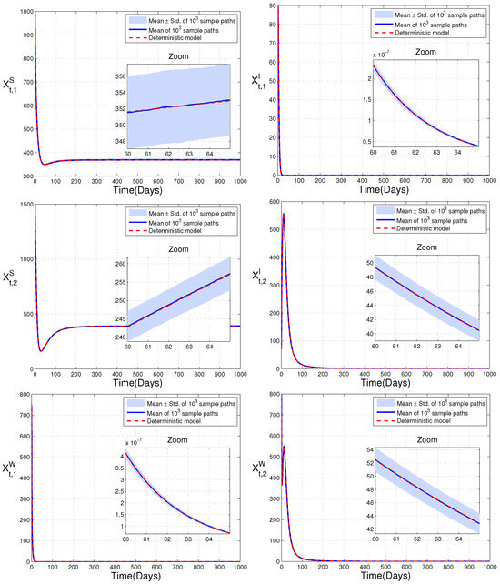
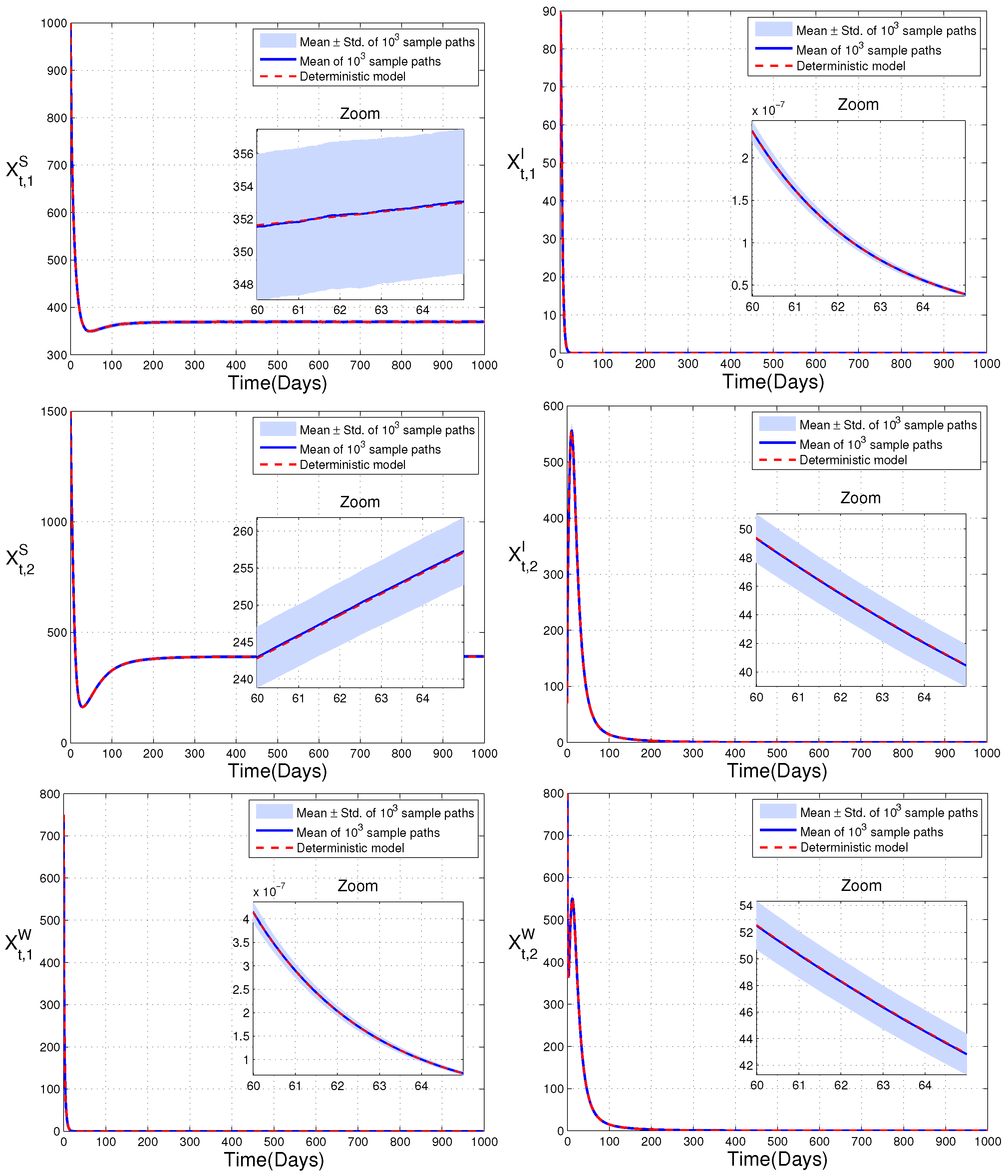
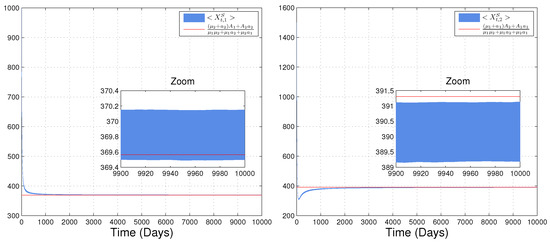
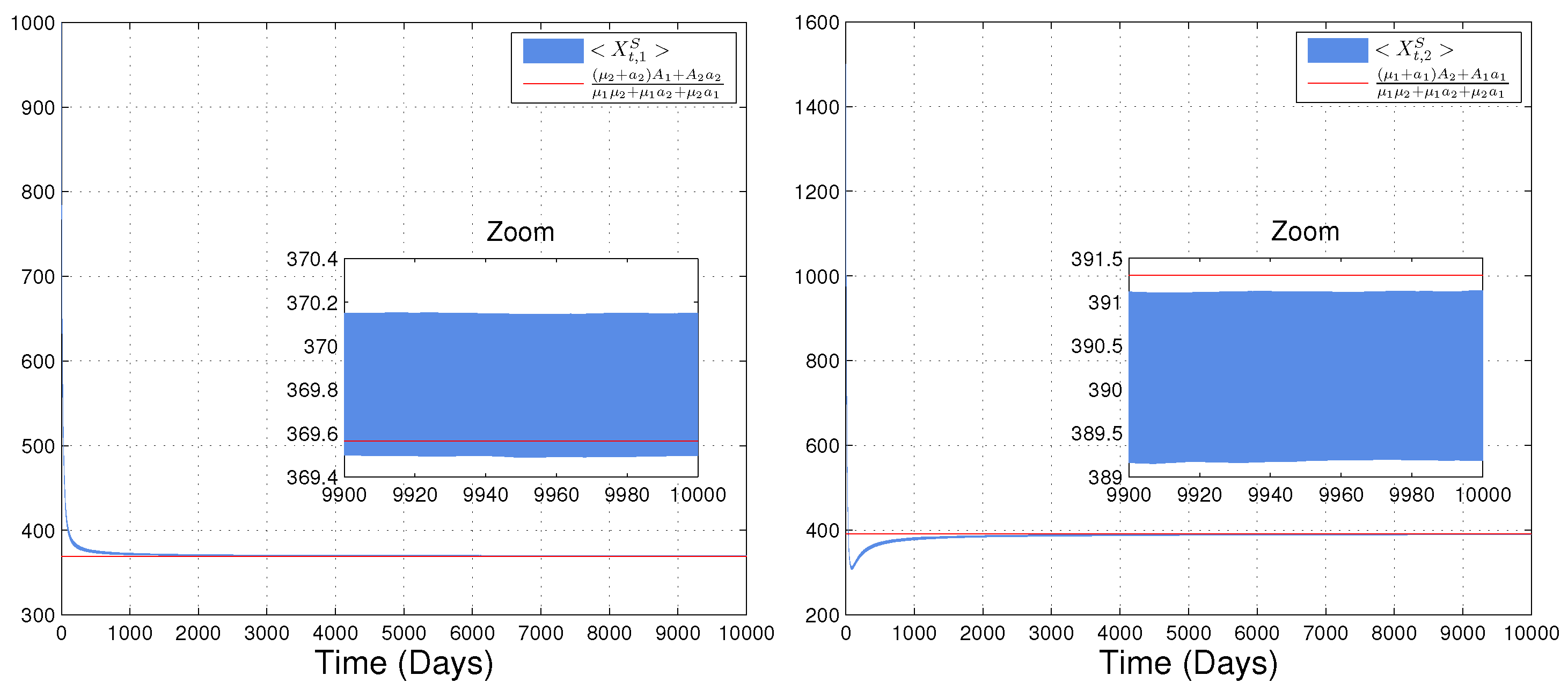
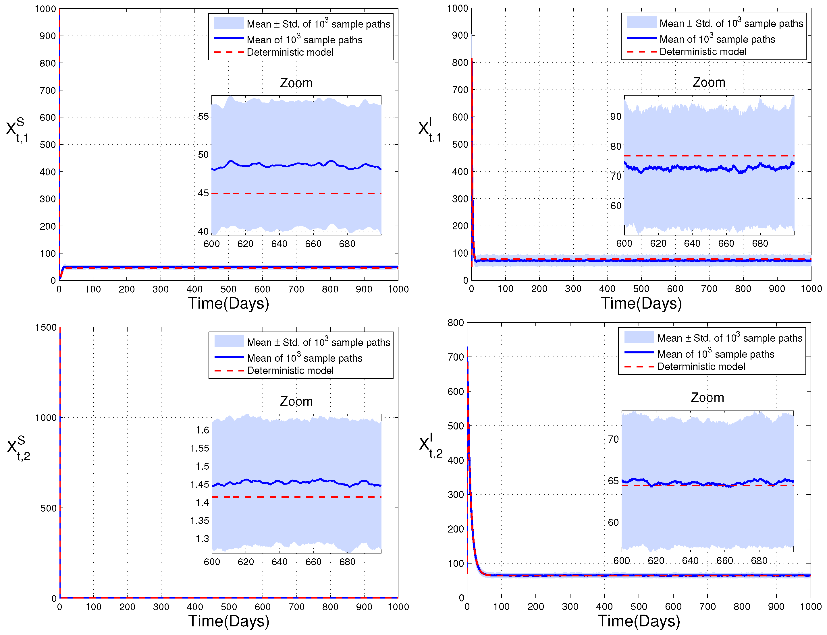
Therefore, all conditions of Theorem 3 are satisfied. To illustrate the theoretical findings of Theorem 3 and compare the deterministic and stochastic dynamics of system (2), we performed numerical simulations using the Milstein scheme (51). For the stochastic model, 1000 independent sample paths were generated. In the first experiment (Figure 1), the final time was set to $T=1000$ with time step $\Delta =0.01$. For each of the six state variables, we plotted (i) the deterministic trajectory, (ii) the sample mean of the 1000 stochastic paths, and (iii) the mean ± one standard deviation. These results show that the stochastic trajectories remain concentrated around their deterministic counterparts and follow the qualitative behavior predicted by the theory. In the second experiment (Figure 2), we examined the long-term time-averaged behavior of ${\mathfrak{X}}_{t,1}^{\mathbb{S}}$ and ${\mathfrak{X}}_{t,2}^{\mathbb{S}}$ up to $T=\mathrm{10,000}$ with the same time step. For each sample path, the time-average quantity

$$\underset{t\to +\infty }{\text{lim}}{\displaystyle \frac{1}{t}}{\int }_0^t{\mathfrak{X}}_{\tau ,i}^{\mathbb{S}}d\tau ,i=1,2,$$

was computed using the trapezoidal rule, and the $5\%-95\%$ quantile bands were plotted. The analytical bounds from Theorem 3 were superimposed for comparison. As the zoomed-in insets show, the empirical time-averaged trajectories converge to their theoretical limits and stay within the analytical bounds, confirming the accuracy and sharpness of Theorem 3.

Figure 1. Stochastic solutions of system (2) and the corresponding deterministic model, computed using the parameter values of Example 1.

Figure 2. Comparison of the processes $⟨{\mathfrak{X}}_{t,i}^{\mathbb{S}}⟩$, $i=1,2$, with their analytical bounds under the parameter set of Example 1.

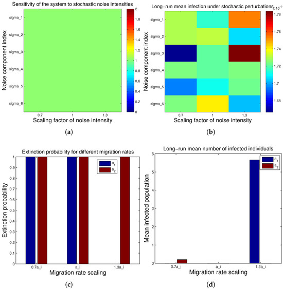
To investigate the effects of noise intensity and migration parameters on the long-term dynamics, additional numerical simulations were performed (Figure 3). The stochastic system was solved using the Milstein scheme, and the results were obtained from 1000 sample paths with time step $\Delta =0.01$ over $[0, 1000]$.

Figure 3. Effects of noise intensities and migration rates on the extinction probability and the long-run mean infection level in system (2) using the parameter values of Example 1. (a) Effect of noise intensities on the extinction probability; (b) effect of noise intensities on the long-run mean infection level; (c) effect of migration rates on the extinction probability; (d) effect of migration rates on the long-run mean infection level.

Figure 3a,b show heatmaps illustrating the sensitivity of the model to variations in noise intensity. The horizontal axis corresponds to the scaling factors $0.7$, $1.0$, $1.3$, and the vertical axis represents the components ${\sigma }_i$, $i=1,\dots ,6$. The color scale indicates the change in the selected model outcome. The nearly uniform patterns suggest that moderate variations in noise intensities do not substantially alter system behavior. Figure 3c shows the extinction probability of the disease for scaled migration parameters $0.7a_i$, $a_i$, and $1.3a_i$, $i=1,2$. The extinction probability remains close to one for all cases, indicating that the disease tends to disappear with high probability under these parameter choices. Figure 3d presents the long-run mean infection level under the same migration scalings. For $0.7a_i$ and $a_i$, the average infection level stays close to zero, while increasing $a_1$ to $1.3a_1$ causes a noticeable rise. In contrast, increasing $a_2$ leads to only a minor change.

Example 2.

We set ${\sigma }_1=0.01$, ${\sigma }_2=0.2$, ${\sigma }_3=0.01$, ${\sigma }_4=0.05$ ${\sigma }_5=0.01$, ${\sigma }_6=0.05$ and parameter values Table 2 with ${\lambda }_1=0.01$, ${\lambda }_2=0.07$. Then, we can calculate that

$$\begin{array}{cc}\hfill R_0^{\left(1\right)}& ={\displaystyle \frac{{\mathcal{A}}_1\left({\lambda }_1{\epsilon }_1+{\beta }_1\left({\epsilon }_1+\frac{{\sigma }_5^2}{2}\right)\right)}{\left(\frac{a_1{\mathcal{A}}_1\left(a_1{\mu }_2+a_2{\mu }_1+{\mu }_1{\mu }_2\right)+\frac{{\sigma }_3^2}{2}({\mu }_1+a_1)({\mathcal{A}}_2({\mu }_1+a_1)+{\mathcal{A}}_1{a}_1)}{a_1({\mathcal{A}}_1({\mu }_2+a_2)+a_2{\mathcal{A}}_2)+\frac{{\sigma }_3^2}{2}({\mathcal{A}}_2({\mu }_1+a_1)+{\mathcal{A}}_1{a}_1)}+\frac{{\sigma }_1^2}{2}\right)\left({\epsilon }_1+\frac{{\sigma }_5^2}{2}\right)\left({\mu }_1+{\delta }_1+{\gamma }_1+\frac{{\sigma }_2^2}{2}\right)}}\hfill \\ \hfill & =1.113419367028875>1,\hfill \\ \hfill R_0^{\left(2\right)}& ={\displaystyle \frac{{\mathcal{A}}_2\left({\lambda }_2{\epsilon }_2+{\beta }_2\left({\epsilon }_2+\frac{{\sigma }_6^2}{2}\right)\right)}{\left(\frac{a_2{\mathcal{A}}_2\left(a_1{\mu }_2+a_2{\mu }_1+{\mu }_1{\mu }_2\right)+\frac{{\sigma }_1^2}{2}({\mu }_2+a_2)({\mathcal{A}}_1({\mu }_2+a_2)+{\mathcal{A}}_2{a}_2)}{a_2({\mathcal{A}}_2({\mu }_1+a_1)+a_1{\mathcal{A}}_1)+\frac{{\sigma }_1^2}{2}({\mathcal{A}}_1({\mu }_2+a_2)+{\mathcal{A}}_2{a}_2)}+\frac{{\sigma }_3^2}{2}\right)\left({\epsilon }_2+\frac{{\sigma }_6^2}{2}\right)\left({\mu }_2+{\delta }_2+{\gamma }_2+\frac{{\sigma }_4^2}{2}\right)}}\hfill \\ \hfill & =1.331802044365130>1,\hfill \end{array}$$

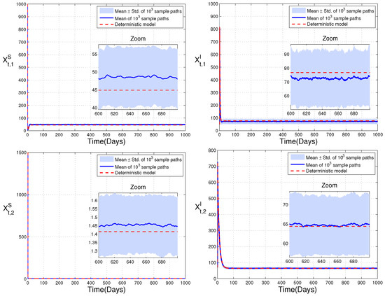
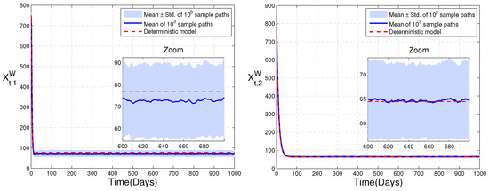
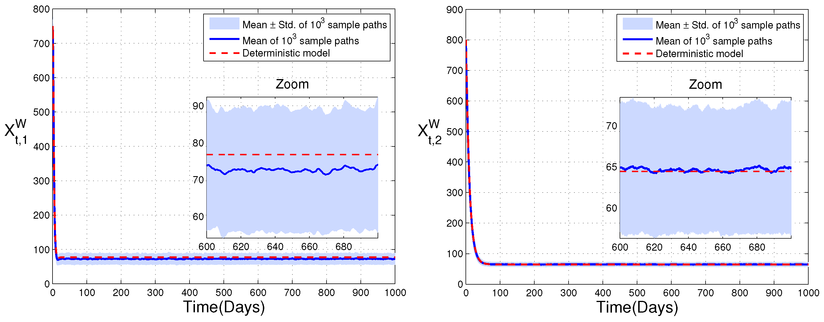
which implies that the condition of Theorem 4 holds. Thus, model (2) has a unique ergodic stationary distribution $\varpi (·)$. Furthermore, we investigate the dynamical behavior of system (2) through numerical simulations. The deterministic counterpart of the model was first solved with a step-size $\Delta =0.01$ and a final time of $T=1000$. In parallel, the stochastic system was simulated using the same time step for 1000 independent sample paths. The results for the six state variables are presented in Figure 4, where the deterministic trajectory, the empirical mean of the 1000 stochastic realizations, and the curves representing the mean together with one standard deviation $(\mathit{mean}\pm \mathit{std.})$ are shown simultaneously. These plots illustrate that the empirical mean of the stochastic system remains close to the deterministic solution and that stochastic fluctuations induced by Gaussian noise do not alter the overall trend of the dynamics, a finding that is consistent with Theorem 4.

Figure 4. Stochastic solutions of system (2) and the corresponding deterministic model, computed using the parameter values of Example 2.

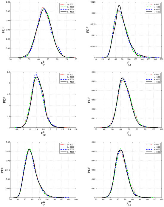
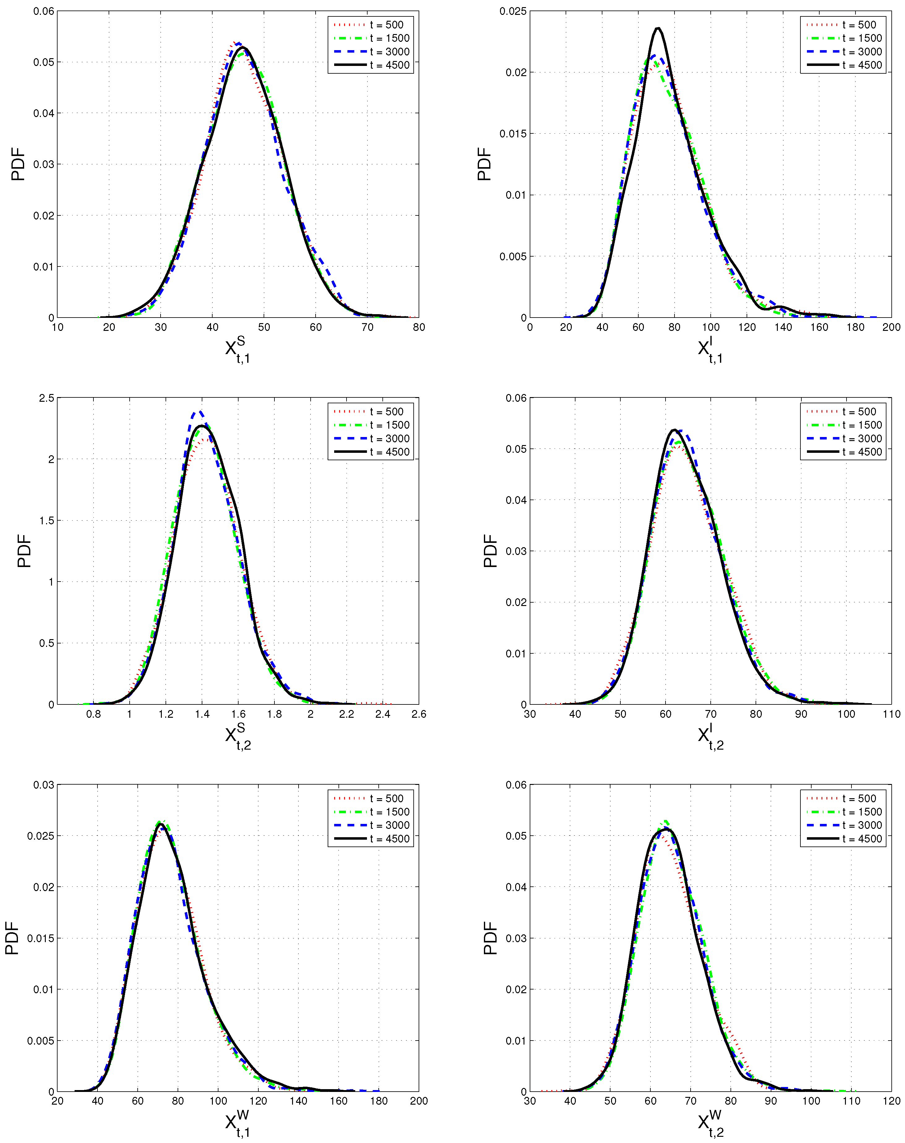
To further examine the probabilistic structure and long-term behavior of the system, we computed the marginal probability density functions (PDFs) of the six state variables at $t=500,1500,3000,4500$ using kernel density estimation applied to the 1000 stochastic trajectories. These results are shown in Figure 5, where the gradual smoothing and stabilization of the probability distributions over time are evident. The empirical convergence of the PDFs in Figure 5, together with the behavior of the sample mean and standard deviation in Figure 4, provides strong numerical support for the theoretical conclusions.

Figure 5. The marginal probability density functions (PDFs) of system (2) at times t = 500, 1500, 300, 4500 using the parameter values of Example 2.

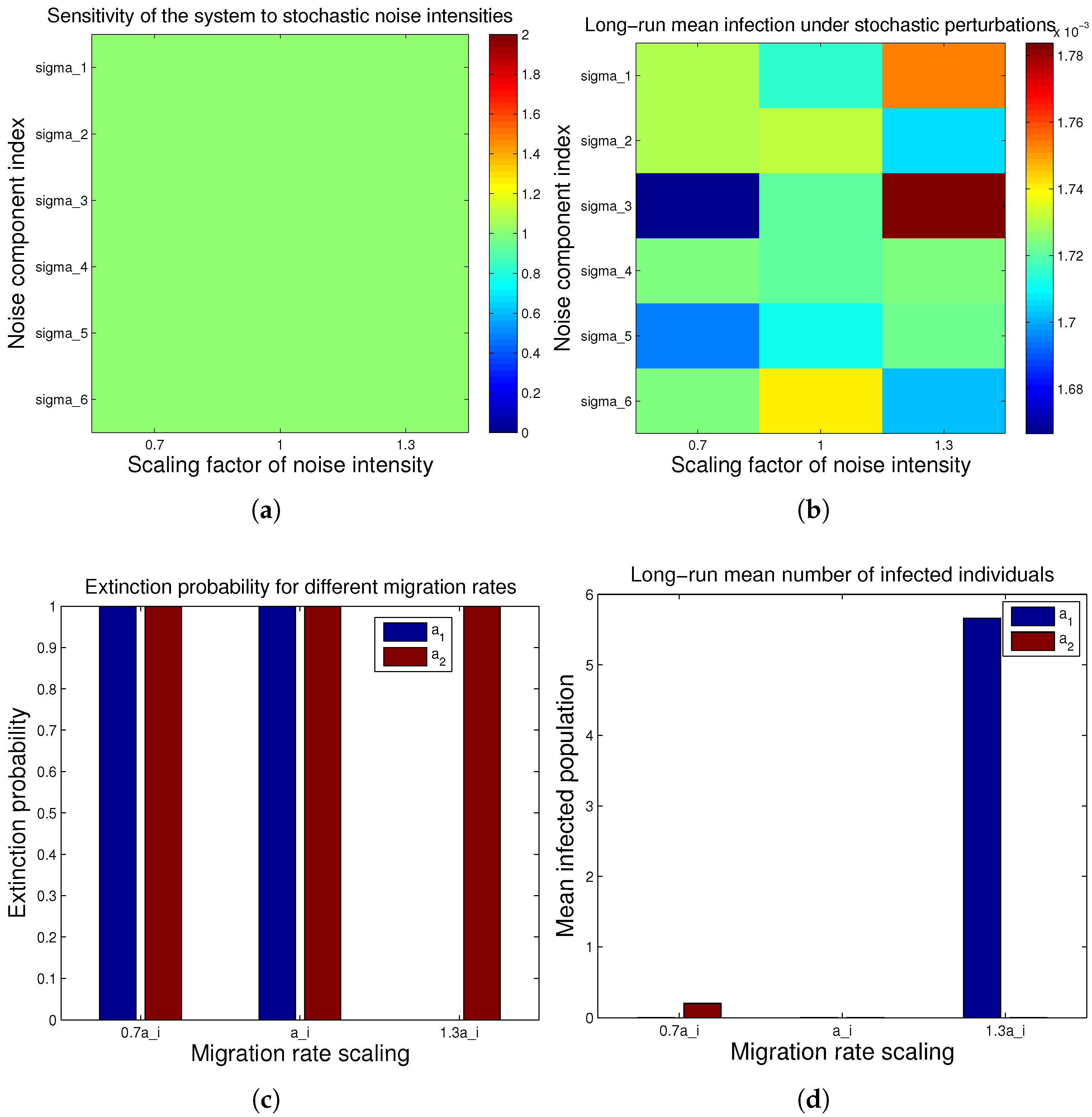
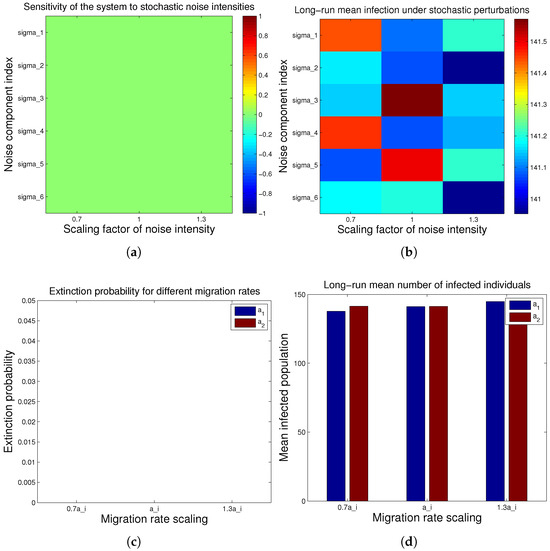
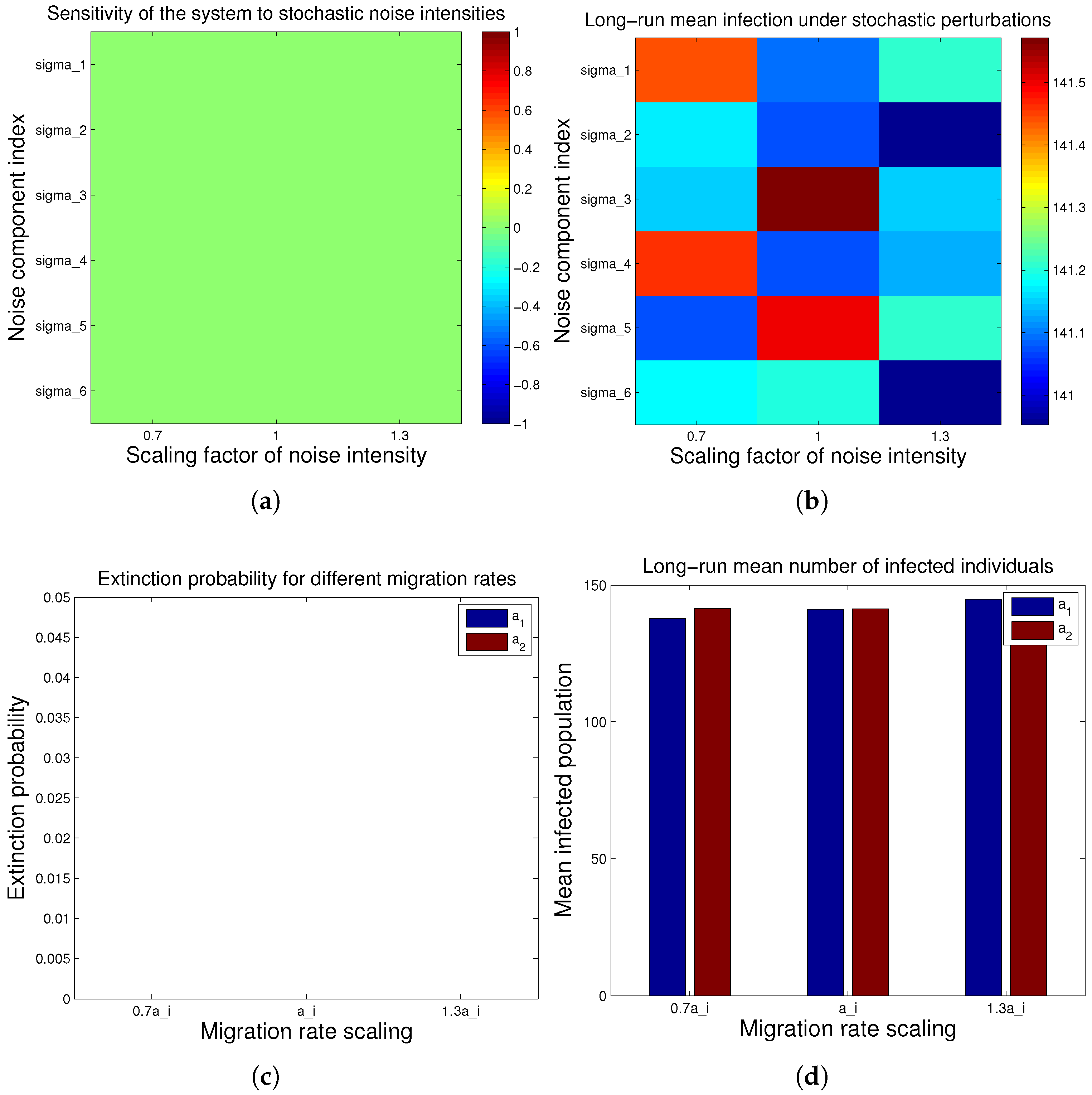
To study the effects of stochastic noise and migration parameters on the long-term behavior, numerical simulations were performed, and the results are presented in Figure 6a–d. Figure 6a presents a sensitivity analysis of the model with respect to the noise intensities. In this figure, the effect of varying each noise component ${\sigma }_i$, $i=1,2,\dots ,6$ is examined using the scaling factors $0.7$, $1.0$, and $1.3$. The relatively uniform color distribution in the heatmap indicates that moderate variations in the noise intensities do not significantly affect the qualitative behavior of the system. Figure 6b illustrates the long-run mean number of infected individuals under different noise intensity scalings. The results show that the average infection level remains approximately constant across the considered range, with only minor quantitative variations.

Figure 6. Effects of noise intensities and migration rates on the extinction probability and the long-run mean infection level in system (2) using the parameter values of Example 2. (a) Effect of noise intensities on the extinction probability; (b) effect of noise intensities on the long-run mean infection level; (c) effect of migration rates on the extinction probability; (d) effect of migration rates on the long-run mean infection level.

The effects of migration parameters on the disease dynamics are investigated in Figure 6c,d. Figure 6c shows the probability of disease extinction for different migration rate scalings. It can be observed that the extinction probability remains close to zero for all considered cases. Finally, Figure 6d presents the long-run mean number of infected individuals for different migration rate scalings. The results indicate that increasing migration rates may lead to a slight increase in the endemic infection level, suggesting that movement between patches can contribute to the persistence of disease transmission in the spatially structured population.

7. Discussion and Conclusions

We develop a stochastic two-patch cholera model with fast-slow transmissions to make the epidemiological effect of environmental stochasticity transparent. In this framework, fast transmission represents the rapid human-to-human infection pathway, while slow transmission captures the indirect environmental route mediated by the pathogen concentration in water. We establish the global existence and uniqueness of the solutions, providing a rigorous mathematical foundation for studying the long-term dynamics of the system. The dependence of $R_0^{\left(1\right)}$ and $R_0^{\left(2\right)}$ on the noise intensities has significant implications for epidemiology. In environments with high variability, such as areas with unstable water quality, irregular sanitation provision, or large variability in human mobility, the reproduction number could be considerably lower than the deterministic value. This finding implies that stochastic noise may influence cholera dynamics such that it increase the probability of disease elimination, depending on the system parameters and noise intensity. Therefore, policies targeting the reduction of environmental variability, such as water infrastructure development, promotion of regular hygiene practices, or reduction of human mobility variability, could have a secondary effect of reducing the risk of disease persistence. In contrast, in more stable environments with lower noise levels, the deterministic value can be used as a safe estimate, and control policies should target established approaches such as vaccination, treatment, and water quality improvement.

The stochastic threshold $R_0=\text{max}\{R_0^{\left(1\right)},R_0^{\left(2\right)}\}$ obtained in Section 5 provides deeper insight into the long-term behavior of the system. If $R_0<1$, the disease goes extinct with probability one independently of the initial conditions. If $R_0>1$, the stochastic process admits a unique stationary distribution, which indicates stochastic persistence. This threshold incorporates the combined effects of demographic stochasticity, environmental variability, and spatial heterogeneity, showing that deterministic predictions may be misleading in finite populations. In particular, in patches with small population size or large variability in contact rates, an outbreak predicted by the deterministic ${\mathcal{R}}_0$ may still fade out due to stochastic effects.

Theorem 4 proves that when $R_0>1$, the stochastic model possesses a unique ergodic stationary distribution. This result implies that the stochastic process converges to a unique invariant probability measure independent of the initial condition, suggesting long-term persistence of the disease in the population. Unlike deterministic models, where $R_0>1$ typically leads to a fixed endemic equilibrium, the stochastic framework captures the natural variability of transmission dynamics. Therefore, the stationary distribution provides information not only about the average endemic level but also about the variability around it, offering a more realistic description of disease dynamics in finite populations. From an epidemiological perspective, this distribution can be used to estimate quantities such as expected prevalence and the probability of extreme outbreaks.

The theoretical results described above are complemented by numerical simulations that illustrate the influence of stochasticity on the system dynamics. In particular, we analyzed the long-term behavior of the stochastic version of system (2) and derived explicit bounds for the time-averaged values of the stochastic components ${\mathfrak{X}}_{t,i}^{\mathbb{S}}$, $i=1,2$. These bounds indicate that although the trajectories may experience noticeable short-term fluctuations, the long-run averaged behavior remains confined within a well-defined region. Such explicit analytical bounds are rarely available for nonlinear stochastic epidemic systems. Figure 1 illustrates the influence of noise on the trajectories of the six state variables. The comparison between the deterministic solution, the sample mean, and the one-standard-deviation band provides intuition about the magnitude of stochastic variability during finite time intervals. The theoretical bounds are further verified in Figure 2, where the time-averaged values of ${\mathfrak{X}}_{t,i}^{\mathbb{S}}$ remain entirely within the predicted analytical limits. This agreement between theory and simulation suggests that the derived bounds accurately describe the system’s long-term time-averaged behavior.

Additional numerical experiments further clarify the influence of parameter variations on disease dynamics. In the parameter regime considered in Example 1, the stochastic reproduction number satisfies $R_0^{*}<1$, and therefore the theoretical results predict disease extinction. This prediction is consistent with the simulation results shown in Figure 3c. The sensitivity analysis with respect to the noise intensities (Figure 3a,b) shows that the system remains relatively robust under moderate stochastic perturbations. Even when migration rates vary, the extinction probability remains very high. However, the long-run mean infection levels displayed in Figure 3d reveal a noticeable sensitivity to directional migration. Increasing the migration parameter $a_1$ leads to a clear rise in the average infection level, whereas variations in $a_2$ produce only minor effects.

A different dynamical behavior is observed in Example 2, where the condition $R_0^{\left(i\right)}>1$, $i=1,2$, holds. According to Theorem 4, the stochastic system admits a unique ergodic stationary distribution in this regime. The simulation results in Figure 4 show that the mean of the 1000 stochastic trajectories closely follows the deterministic solution, while the standard deviations indicate fluctuations around this trend. Additional confirmation is provided in Figure 5, where the marginal probability density functions gradually stabilize and approach a stationary profile over time. These results demonstrate the convergence of the system to its stationary distribution and confirm the theoretical predictions.

The sensitivity analysis presented in Figure 6a,b indicates that moderate changes in the noise intensities ${\sigma }_i$ do not substantially alter the qualitative dynamics of the model. Instead, stochastic perturbations mainly introduce fluctuations around the endemic equilibrium. In contrast, migration parameters have a more pronounced effect on the infection level. As shown in Figure 6c, the extinction probability remains close to zero for all considered migration scalings, confirming that elimination is unlikely when $R_0^{\left(i\right)}>1$. Moreover, Figure 6d shows that increasing migration rates slightly raises the long-run mean number of infected individuals, suggesting that population mobility contributes to maintaining disease persistence in spatially structured populations.

The results obtained in this study, both theoretical and numerical, consistently demonstrate the essential role of stochastic fluctuations in shaping the long-term dynamics of the system, including extinction and persistence behavior.

It is important to note that environmental stochasticity in the present model is incorporated directly into the system equations through multiplicative noise rather than through parameter fluctuations such as transmission or shedding rates. While this approach provides a tractable representation of uncertainty across all state variables, further biological insights could be obtained by introducing parameter-specific stochasticity. For example, environmental variability may affect contact rates, recovery rates, or pathogen decay rates in different ways. Exploring such mechanisms represents a promising direction for future research.

Another modeling assumption concerns pathogen dispersal between patches. Following the framework of Berge et al. [18], pathogen movement occurs only through human migration and not through water transport. Although this assumption allows a clear analysis of human-mediated transmission, it may not be appropriate in regions where hydrological connectivity plays a major role. Previous studies have shown that river systems or irrigation networks can significantly influence cholera spread. Therefore, incorporating hydrodynamic transport into the model represents an important extension for future work.

Finally, it should be emphasized that the parameter values used in the numerical simulations are not estimated from real epidemiological data. The simulations are intended primarily to illustrate the theoretical results, including the extinction threshold and the ergodic stationary distribution. The deterministic parameters were selected within biologically plausible ranges commonly used in the cholera modeling literature, while the noise intensities were varied to examine the effects of environmental heterogeneity. Future work could extend the present framework by estimating both deterministic parameters and stochastic intensities from observational data.

The results of the proposed stochastic two-patch cholera model have practical implications for regions characterized by strong environmental variability. In many endemic settings, environmental fluctuations influence the concentration of Vibrio cholerae in water sources and can amplify or suppress transmission dynamics. Our analysis suggests that when transmission potential differs between connected patches, targeted interventions focused on high-transmission locations may be more effective than uniform strategies. Such interventions may include intensified water treatment, sanitation improvements, or enhanced surveillance during periods of elevated environmental risk. Empirical studies have similarly shown that spatially targeted water and sanitation interventions can substantially reduce cholera incidence in heterogeneous environments [40,41].

Several simplifying assumptions should also be acknowledged. The model does not explicitly include seasonal forcing, despite evidence that cholera transmission is often strongly seasonal [42,43]. In addition, asymptomatic infections are not considered, although they may contribute to environmental contamination [44,45]. Finally, the environmental component of the model represents bacterial dynamics in a simplified form and does not capture complex hydrological processes. Addressing these limitations by incorporating seasonal drivers, additional epidemiological compartments, and data-driven parameter estimation would further enhance the model’s predictive capacity.

References

- Zhou, X. Dynamical Analysis of a Stochastic Cholera Epidemic Model. Mathematics 2022, 10, 2830. [Google Scholar] [CrossRef] [Scilit]
- Calatayud, J.; Cortés, J.C.; Dorini, F.A.; Jornet, M. Dealing with variability in ecological modelling: An analysis of a random non-autonomous logistic population model. Math. Methods Appl. Sci. 2022, 45, 3318–3333. [Google Scholar]
- Brhane, K.W.; Ahmad, A.G.; Hina, H.; Emadifar, H. Mathematical modeling of cholera dynamics with intrinsic growth considering constant interventions. Sci. Rep. 2024, 14, 4616. [Google Scholar] [CrossRef] [Scilit] [PubMed]
- Torkzadeh, L.; Fahimi, M.; Ranjbar, H.; Nouri, K. Analysis of a stochastic model for a prey–predator system with an indirect effect. Int. J. Comput. Math. 2025, 102, 60–73. [Google Scholar]
- World Health Organization, Cholera. 2023. Available online: http://www.who.int/news-room/fact-sheets/detail/cholera (accessed on 24 May 2026).
- Capasso, V.; Paveri-Fontana, S. A mathematical model for the 1973 cholera epidemic in the European Mediterranean region. Rev. Epidemiol. Sante Publique 1979, 27, 121–132. [Google Scholar] [PubMed]
- Codeço, C.T. Endemic and epidemic dynamics of cholera: The role of the aquatic reservoir. BMC Infect. Dis. 2001, 1, 1–14. [Google Scholar] [CrossRef] [Scilit] [PubMed]
- Hartley, D.M.; Morris, J.J.G.; Smith, D.L. Hyperinfectivity: A criticalelement in the ability of v.cholerae to cause epidemics? PLoS Med. 2006, 3, e7. [Google Scholar] [PubMed]
- Sharma, S.; Singh, F. Bifurcation and stability analysis of a cholera model with Vaccination and saturated treatment. Chaos Solitons Fractals 2021, 146, 110912. [Google Scholar] [CrossRef] [Scilit]
- Misra, A.K.; Gupta, A.; Venturino, E. Cholera dynamics with bacteriophage infection: A mathematical Study. Chaos Solitons Fractals 2016, 91, 610–621. [Google Scholar] [CrossRef] [Scilit]
- Cai, L.; Li, Z.; Yang, C.; Wang, J. Global analysis of an environmental disease transmission model linking within-host and between-host dynamics. Appl. Math. Model. 2020, 86, 404–423. [Google Scholar] [PubMed]
- Tian, X.; Xu, R.; Lin, J. Mathematical analysis of a cholera infection model with vaccination strategy. Appl. Math. Comput. 2019, 361, 517–535. [Google Scholar] [CrossRef] [Scilit]
- Medda, R.; Tiwari, P.K.; Pal, S. Impacts of planktonic components on the dynamics of cholera epidemic: Implications from a mathematical model. Math. Comput. Simul. 2024, 219, 505–526. [Google Scholar]
- Eisenberg, M.C.; Shuai, Z.; Tien, J.H.; van den Driessche, P. A cholera model in a patchy environment with water and human movement. Math. Biosci. 2013, 246, 105–112. [Google Scholar] [CrossRef] [Scilit] [PubMed]
- Bertuzzo, E.; Azaele, S.; Maritan, A.; Gatto, M.; Rodriguez-Iturbe, I.; Rinaldo, A. On the space-time evolution of a cholera epidemic. Water Resour. Res. 2008, 44, W01424. [Google Scholar] [CrossRef] [Scilit]
- Zhou, X.Y.; Cui, J.A. Threshold dynamics for a cholera epidemic model with periodic transmission rate. Appl. Math. Model. 2013, 37, 3093–3101. [Google Scholar] [CrossRef] [Scilit]
- Njagarah, J.B.H.; Nyabadza, F. A metapopulation model for cholera transmission dynamics between communities linked by migration. Appl. Math. Comput. 2014, 241, 317–331. [Google Scholar] [CrossRef] [Scilit]
- Berge, T.; Bowong, S.; Lubuma, J.M.S. Global stability of a two-patch cholera model with fast and slow transmissions. Math. Comput. Simul. 2017, 133, 142–164. [Google Scholar] [CrossRef] [Scilit]
- Cheng, X.; Wang, Y.; Huang, G. Dynamics of cholera transmission model with imperfect vaccination and demographics on complex networks. J. Frankl. Inst. 2023, 360, 1077–1105. [Google Scholar]
- Anteneh, L.M.; Lokonon, B.E.; Glèlè Kakaï, R. Modelling techniques in cholera epidemiology: A systematic and critical review. Math. Biosci. 2024, 373, 109210. [Google Scholar] [CrossRef] [Scilit] [PubMed]
- Liu, Q.; Jiang, D.; Hayat, T.; Alsaedi, A. Dynamical behavior of a stochastic epidemic model for cholera. J. Frankl. Inst. 2019, 356, 7486–7514. [Google Scholar] [CrossRef] [Scilit]
- Tilahun, G.T.; Woldegerima, W.A.; Wondifraw, A. Stochastic and deterministic mathematical model of cholera disease dynamics with direct transmission. Adv. Differ. Equ. 2020, 2020, 670. [Google Scholar] [CrossRef] [Scilit]
- Allen, L.J.S.; Wang, X. Stochastic models of infectious diseases in a periodic environment with application to cholera epidemics. J. Math. Biol. 2021, 82, 48. [Google Scholar] [CrossRef] [Scilit] [PubMed]
- Witbooi, P.J.; Muller, G.E.; Ongansie, M.B.; Ahmed, I.H.I.; Okosun, K.O. A stochastic population model of cholera disease. Discret. Contin. Dyn. Syst. Ser. S 2022, 15, 441–456. [Google Scholar] [CrossRef] [Scilit]
- Song, Y.; Liu, P.; Din, A. Analysis of a stochastic epidemic model for cholera disease based on probability density function with standard incidence rate. AIMS Math. 2023, 8, 18251–18277. [Google Scholar] [CrossRef] [Scilit]
- Liu, Q.; Jiang, D. Stationary distribution of a stochastic cholera model with imperfect vaccination. Physical A 2020, 550, 124031. [Google Scholar] [CrossRef] [Scilit]
- Liu, Q.; Jiang, D.; Hayat, T.; Alsaedi, A.; Ahmad, B. Stationary distribution of a stochastic cholera model between communities linked by migration. Appl. Math. Comput. 2020, 373, 125021. [Google Scholar] [CrossRef] [Scilit]
- Song, M.; Zuo, W.; Jiang, D.; Hayat, T. Stationary distribution and ergodicity of a stochastic cholera model with multiple pathways of transmission. J. Frankl. Inst. 2020, 357, 10773–10798. [Google Scholar] [CrossRef] [Scilit]
- Zhou, X.; Shi, X.; Wei, M. Dynamical behavior and optimal control of a stochastic Mathematical model for cholera. Chaos Solitons Fractals 2022, 156, 111854. [Google Scholar] [CrossRef] [Scilit]
- Zhu, Y.; Wang, L.; Qiu, Z. Dynamics of a stochastic cholera epidemic model with Lévy process. Physical A 2022, 595, 127069. [Google Scholar] [CrossRef] [Scilit]
- Vezzulli, L.; Grande, C.; Reid, P.C.; Hélaouët, P.; Edwards, M.; Höfle, M.G.; Brettar, I.; Colwell, R.R.; Pruzzo, C. Climate influence on Vibrio and associated human diseases during the past half-century in the coastal North Atlantic. Proc. Natl. Acad. Sci. USA 2016, 113, 5062–5071. [Google Scholar] [CrossRef] [Scilit]
- Escobar, L.E.; Ryan, S.J.; Stewart-Ibarra, A.M.; Finkelstein, J.L.; King, C.A.; Qiao, H.; Polhemus, M.E. A global map of suitability for coastal Vibrio cholerae under current and future climate conditions. Acta Trop. 2015, 149, 202–211. [Google Scholar] [CrossRef] [Scilit] [PubMed]
- Lessler, J.; Moore, S.M.; Luquero, F.J.; McKay, H.S.; Grais, R.; Henkens, M.; Mengel, M.; Dunoyer, J.; M’bangombe, M.; Lee, E.C.; et al. Mapping the burden of cholera in sub-Saharan Africa and implications for control: An analysis of data across geographical scales. Lancet 2018, 391, 1908–1915. [Google Scholar] [CrossRef] [Scilit] [PubMed]
- Ali, M.; Nelson, A.R.; Lopez, A.L.; Sack, D.A. Updated global burden of cholera in endemic countries. PLoS Neglected Trop. Dis. 2015, 9, e0003832. [Google Scholar] [CrossRef] [Scilit]
- Wesolowski, A.; Buckee, C.O.; Engø-Monsen, K.; Metcalf, C.J.E. Connecting mobility to infectious diseases: The promise and limits of mobile phone data. J. Infect. Dis. 2016, 214, 414–420. [Google Scholar] [CrossRef] [Scilit]
- Kraemer, M.U.; Yang, C.H.; Gutierrez, B.; Wu, C.H.; Klein, B.; Pigott, D.M.; Group†, O.C.D.W.; Du Plessis, L.; Faria, N.R.; Li, R.; et al. The effect of human mobility and control measures on the COVID-19 epidemic in China. Science 2020, 368, 493–497. [Google Scholar] [CrossRef] [Scilit] [PubMed]
- Mao, X. Stochastic Differential Equations and Applications, 2nd ed.; Horwood Publishing Limited: Chichester, UK, 2008; p. xviii+422. [Google Scholar]
- Khasminskii, R. Stochastic Stability of Differential Equations, 2nd ed.; Stochastic Modelling and Applied Probability; Springer: Berlin/Heidelberg, Germany, 2012; Volume 66, p. xviii+339. [Google Scholar]
- Milstein, G.N.; Tretyakov, M.V. Stochastic Numerics for Mathematical Physics; Scientific Computation; Springer: Berlin/Heidelberg, Germany, 2004; p. xx+594. [Google Scholar]
- D’Mello-Guyett, L.; Gallandat, K.; Van den Bergh, R.; Taylor, D.; Bulit, G.; Legros, D.; Maes, P.; Checchi, F.; Cumming, O. Prevention and control of cholera with household and community water, sanitation and hygiene (WASH) interventions: A scoping review of current international guidelines. PLoS ONE 2020, 15, e0226549. [Google Scholar] [CrossRef] [Scilit] [PubMed]
- Bwire, G.; Kisakye, A.; Amulen, E.; Bwanika, J.B.; Badebye, J.; Aanyu, C.; Nakirya, B.D.; Okello, A.; Okello, S.A.; Bukenya, J.N.; et al. Cholera and COVID-19 pandemic prevention in multiple hotspot districts of Uganda: Vaccine coverage, adverse events following immunization and WASH conditions survey. BMC Infect. Dis. 2023, 23, 487. [Google Scholar] [CrossRef] [Scilit] [PubMed]
- Asadgol, Z.; Badirzadeh, A.; Niazi, S.; Mokhayeri, Y.; Kermani, M.; Mohammadi, H.; Gholami, M. How climate change can affect cholera incidence and prevalence? A systematic review. Environ. Sci. Pollut. Res. 2020, 27, 34906–34926. [Google Scholar] [CrossRef] [Scilit]
- Moore, S.M.; Azman, A.S.; Zaitchik, B.F.; Mintz, E.D.; Brunkard, J.; Legros, D.; Hill, A.; McKay, H.; Luquero, F.J.; Olson, D.; et al. El Niño and the shifting geography of cholera in Africa. Proc. Natl. Acad. Sci. USA 2017, 114, 4436–4441. [Google Scholar] [CrossRef] [Scilit] [PubMed]
- Richterman, A.; Sainvilien, D.R.; Eberly, L.; Ivers, L.C. Individual and household risk factors for symptomatic cholera infection: A systematic review and meta-analysis. J. Infect. Dis. 2018, 218, S154–S164. [Google Scholar] [CrossRef] [Scilit] [PubMed]
- King, A.A.; Ionides, E.L.; Pascual, M.; Bouma, M.J. Inapparent infections and cholera dynamics. Nature 2008, 454, 877–880. [Google Scholar] [CrossRef] [Scilit] [PubMed]
Disclaimer/Publisher’s Note: The statements, opinions and data contained in all publications are solely those of the individual author(s) and contributor(s) and not of MDPI and/or the editor(s). MDPI and/or the editor(s) disclaim responsibility for any injury to people or property resulting from any ideas, methods, instructions or products referred to in the content. |
© 2026 by the authors. Licensee MDPI, Basel, Switzerland. This article is an open access article distributed under the terms and conditions of the Creative Commons Attribution (CC BY) license.