


Abstract
Source-Seeking in unknown scalar fields is a fundamental problem in robotics with applications in environmental monitoring and disaster response. In this work, we present a source-seeking approach with non-reversing forward velocity regulation by fusing measurement data from multiple sensors within the Stochastic Extremum Seeking (SES) framework. Specifically, a device model with multiple sensors is first constructed, and then a velocity regulation scheme is designed by leveraging the boundedness of the hyperbolic tangent function and the non-negativity of the exponential function to guarantee strictly positive forward velocity. We then evaluate the algorithm both in simulation environments and on the real-world Two-Wheeled Differential Drive Robot platform. The experiments show that our approach not only ensures the forward velocity remains non-negative, aligning with the design expectation, but also accurately locates the source. This work provides new insights into the design of velocity regulation strategies within the SES framework.
MSC:
93E35; 93C85
1. Introduction
A key research area in source localization involves the use of mobile robots to identify and analyze environmental signals, like radio waves or chemical gases, to determine the location of an unknown emission source or leak point [1,2,3]. The significance lies in its ability to achieve automated, efficient source detection in hazardous, complex, or satellite-denied environments [4].
To locate the source, the onboard algorithm should extract gradient information from scalar field measurements and translate this information into effective control commands for the source-seeking platform’s motors [5,6]. Among the various approaches developed to meet these stringent requirements, Extremum Seeking (ES) control has emerged as one of the most popular and powerful techniques, yet its core implementation remains remarkably simple. This method involves adding a small periodic perturbation to the vehicle’s motion and correlating it with the resulting changes in the measured signal [7,8,9,10]. Based on ES and stochastic process theory, Liu and Krstic introduced the Stochastic Extremum Seeking (SES) control method in 2010 [11]. This approach uses colored noise as the excitation signal, in contrast to the sinusoidal excitation signal employed in ES.
In this work, we focus on strategies for regulating forward velocity within the ES and SES frameworks. One approach involves maintaining the forward velocity of a source-seeking device at a constant value. This results in the vehicle continuously orbiting the source once it is located, as demonstrated by algorithms [11,12,13,14]. The other approach couples the velocity with real-time sensor measurements [15,16,17,18,19,20]. This strategy gradually reduces the forward velocity as the device approaches the source, allowing it to move either at a very low speed near the source or come to a complete stop exactly at the source location. While some methods maintain a constant angular velocity regulation [15,17,18], others vary it based on sensor readings [16,19,20].
In reviewing the aforementioned sensor-based velocity regulation approaches, we observe a subtle but noteworthy phenomenon: the forward velocity of the device may become negative under the action of the control law. In terms of actual kinematic behavior, this implies that the vehicle gradually decelerates from forward motion to a complete stop, and subsequently begins to move in reverse. While this phenomenon is kinematically admissible and does not compromise the fundamental objective of source-seeking, the resulting forward-reverse switching inevitably introduces unnecessary trajectory tortuosity and temporal overhead. This observation prompts us to explore whether the properties of fundamental mathematical functions can provide a simple solution to this issue.
Using multi-sensor fusion to enhance the performance of control algorithms is a common technique in engineering practice [21,22]. In the case of source-seeking devices, integrating multiple sensors provides richer environmental information, which has facilitated the development of various multi-agent source localization techniques [23,24]. However, compared to controlling a single device, employing swarm techniques to manage source-seeking devices introduces significantly greater complexity. This motivates us to investigate how multiple sensors can be mounted on a single vehicle to capture essential spatial information while preserving the simplicity of single-device control.
In this study, we propose a straightforward yet effective approach for source-seeking using a single vehicle. The vehicle is equipped with two sensors mounted in tandem along its forward direction. This configuration captures essential spatial information while avoiding the coordination challenges typical of multi-agent systems. For forward velocity control, we use multi-sensor fusion combined with the continuous and bounded nature of the hyperbolic tangent function, as well as the non-negative property of exponential functions. For angular velocity regulation, we build on the beneficial attributes of the SES method. We validate our approach both in simulation and on a physical robotic platform. Experimental results show that our algorithm successfully achieves the source-seeking objective.
2. Related Works
2.1. Source-Seeking Problem
A source-seeking problem refers to the task of locating an unknown source using an autonomous device that operates without prior knowledge of the environment or its own position, relying only on real-time sensor measurements to guide its motion. The problem assumes that the signal field f generated by a source at decreases monotonically with distance, with peak intensity . Sensors can measure signal strength at any location and time, satisfying , where represents the sensor position. The objective is to guide the device to the source location as quickly as possible.
In this study, we mainly adopt an anisotropic signal field:
where control the spatial decay rates along the x and y directions, respectively.
2.2. Two-Wheeled Differential Drive Robot Platform
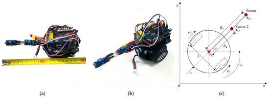
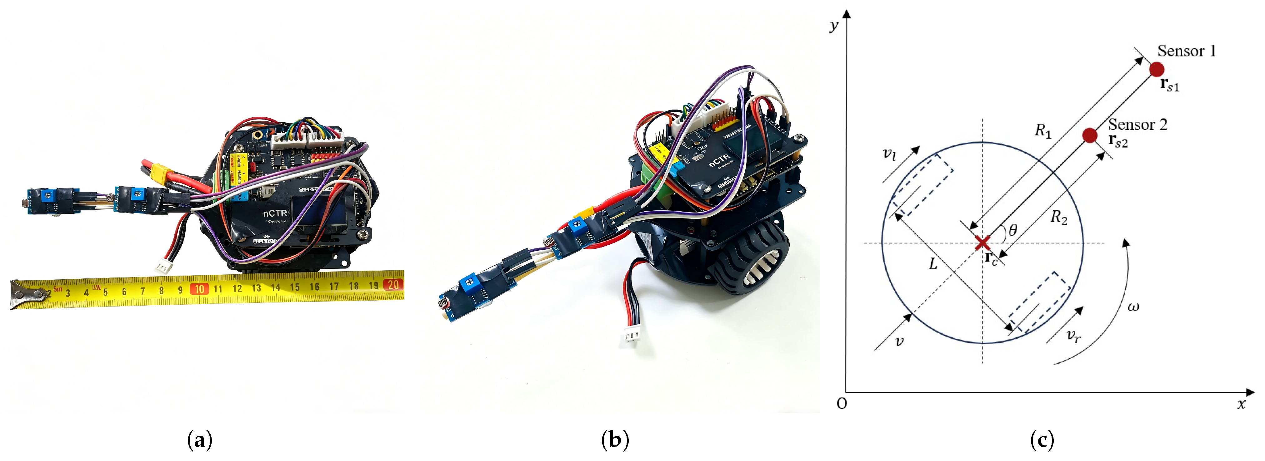
We employ a Two-Wheeled Differential Drive Robot (TWDDR) platform, depicted in Figure 1a,b, as our source-seeking platform. And its geometric interpretation of the kinematic model is shown in Figure 1c.
Figure 1.
TWDDR platform and its simplified model: (a) Overlook view. (b) Strabismus view. (c) Geometric interpretation of the kinematic model for the TWDDR.
The TWDDR is defined by its Cartesian coordinates and heading angle . The distance between the two wheels is cm, and the robot’s motion is controlled by linear and angular velocities at the center point, with the left and right wheel velocities denoted by and , respectively. The kinematic equations for velocity conversion and pose update are provided in Appendix A. Additional hardware details can be found in Appendix B.
Two sensors are mounted along the robot’s longitudinal axis at distances cm and cm from the center point . Their Cartesian coordinates and are related to the robot’s center by:
2.3. Perspectives from Causal Inference and Machine Learning
Beyond traditional source-seeking control, recent advances in causal inference and out-of-distribution generalization offer potential insights for handling environmental uncertainties [25,26,27]. Additionally, sequence modeling techniques such as Transformers with in-context learning [28] could inspire future work on online adaptation of source-seeking parameters. While these perspectives are not integrated into the current stochastic extremum seeking framework, they point to possible directions for more robust and data-efficient source localization.
3. Algorithm Design
3.1. Forward Velocity Control Scheme
Let be the output of the washout filter applied to the sensor reading for . To dynamically adjust the forward speed, we employ the following velocity control law:
where represents the initial speed, and denotes the actual speed of the device at time t after dynamic adjustment based on sensor feedback, k is a positive constant that regulates the sensitivity of speed variation.
The design of Equation (5) follows a multiplicative modulation philosophy: the baseline speed is scaled by a positive factor determined by the sensor feedback, rather than being additively corrected by a term proportional to the sensor difference as in many conventional approaches. The mechanism of this dynamic adjustment is primarily governed by the function, which offers critical advantages for ensuring both smooth velocity modulation and the prevention of reverse motion:
- Smooth saturation. As the sensor difference varies, continuously maps the input to the range , preventing extreme sensor readings from causing uncontrolled velocity fluctuations. Moreover, near equilibrium, responds approximately linearly with a slope near unity, allowing sensitive adjustments when the difference between the two sensor measurements is small.
- Non-negativity guarantee. In the extreme case where the Sensor 2’s signal far exceeds the Sensor 1’s signal (), approaches but never goes below it. Consequently, the exponent is always greater than . Substituting into the exponential function:This guarantees that remains strictly positive for all possible sensor readings. The device can slow down significantly when moving away from the source, but it will never come to a complete stop or reverse direction in the worst situation.
Defining at time t, the velocity response satisfies the following properties:
- When , it indicates that the vehicle’s heading points toward the source direction to some extent. In this case, , so the velocity increases, accelerating the vehicle toward the source.
- When , it indicates that the vehicle’s heading deviates from the source direction to some extent. In this case, , so the velocity decreases, slowing down the vehicle to allow for steering adjustment toward the source.
- When , it indicates that the vehicle may be located in a region with no gradient variation (i.e., the sensor readings from both sides are equal). In this case, , so the velocity remains at the initial speed , and the vehicle continues cruising at its current speed.
3.2. Angular Velocity Control Scheme
The vehicle’s angular velocity control law is defined by Equation (7):
where is the amplitude gain of the colored noise , which is used to persistently excite the system for gradient estimation; is the gain of the demodulated signal , which determines the sensitivity of the angular velocity to the estimated gradient of the unknown field; is a colored noise generated by passing a white noise (W is a standard Brownian motion defined in a probability space with the sample space , the -field and the probability measure ) through a high-pass filter, satisfying Equation (8):
The procedure for generating colored noise from white noise is described as follows:
In the design of the angular velocity control law, only a single sensor is utilized. From a physical structure perspective, the rotational motion of the device exhibits axial symmetry, so measurements from one sensor suffice to provide the instantaneous orientation increment needed for angular velocity regulation. However, a mathematical justification exists for preferentially using Sensor 1 over Sensor 2.
Consider the unknown scalar field generated by the source. Sensor i () ’s measurement is therefore
For sufficiently small relative to the spatial variation of the field, a first-order Taylor expansion around gives
where denotes the directional derivative of the field along the vehicle’s heading.
In our angular velocity control law, the demodulated signal is derived exclusively from Sensor 1. According to the stochastic extremum seeking framework, the expected value of is proportional to the product of the sensor offset and the directional derivative:
Thus, the effective gradient estimate available to the controller scales linearly with . Meanwhile, the signal-to-noise ratio (SNR) for gradient estimation, assuming independent and identically distributed measurement noise with variance , satisfies
Because in our hardware configuration, we obtain . Hence, Sensor 1 provides strictly higher sensitivity to the local gradient than Sensor 2.
3.3. Summary of Algorithm
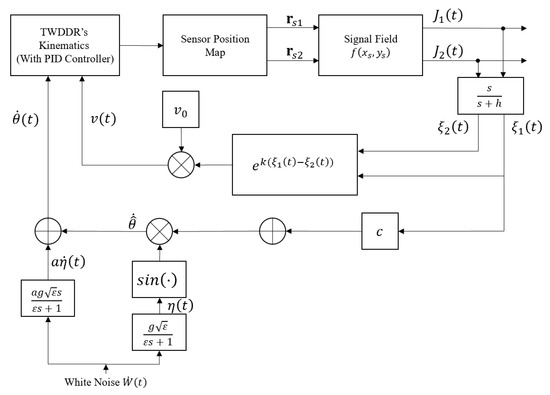
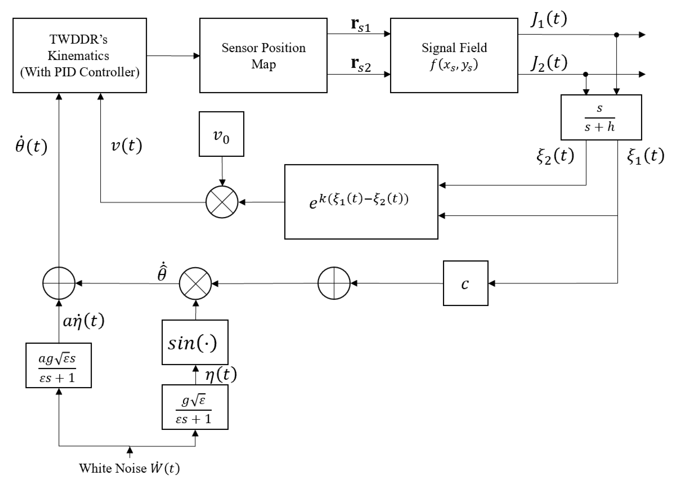
By combining the forward velocity control law and the angular velocity control law, the block diagram of the proposed algorithm is presented in Figure 2. The key parameters are , , k, and , which directly affect convergence speed and localization accuracy. The remaining parameters a, c, g, , h are secondary; their selection can follow the guidelines in [11], and they have relatively minor impact within typical ranges.
Figure 2.
Block diagram of the control algorithm.
Incorporating the kinematic update equations, the algorithm can be expressed as follows:
where is the initial heading angle of vehicle, and denotes the dummy time variable ranging over the integration interval .
4. Simulation Experiment
4.1. Simulation Experiment 1: Baseline Performance
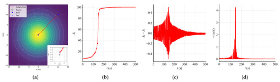
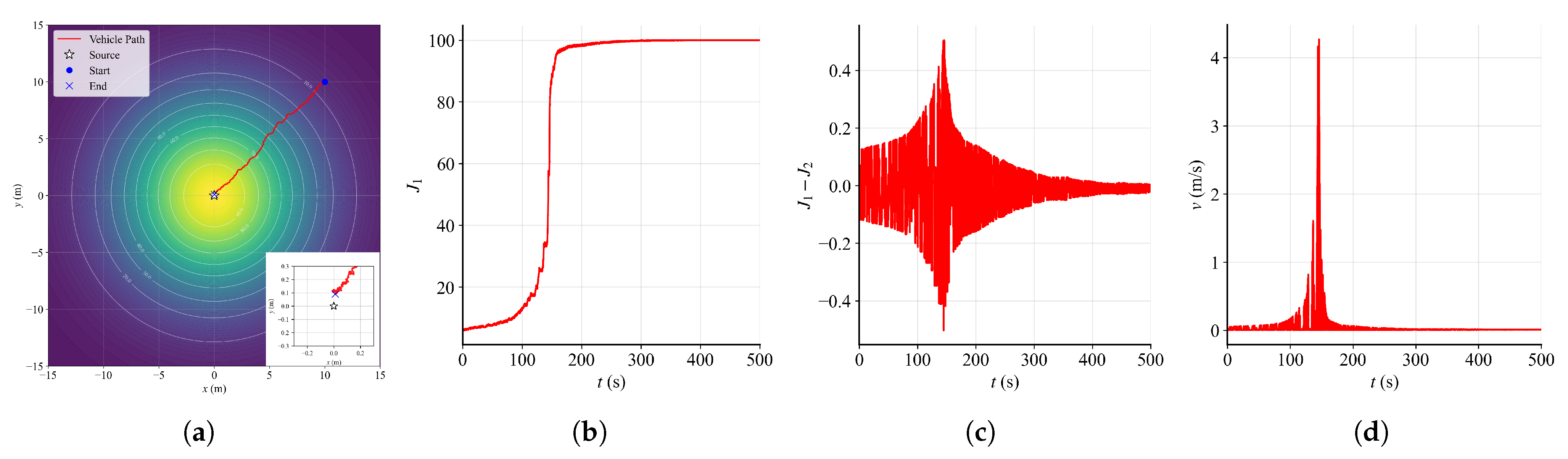
Set , , and total simulation time s, and initialize the vehicle at with m/s, m and m. The other parameters are , , , , . The simulation result is shown in Figure 3.
Figure 3.
Simulation Experiment 1 result: (a) Panoramic view of the device movement trajectory and a close-up view of the trajectory near the source. (b) as a function of time. (c) Sensors reading difference as a function of time. (d) v as a function of time.
Figure 3 shows that after activation, the vehicle moves rapidly toward the source along the radial direction. At approximately s, the vehicle approaches the source and gradually reduces its speed. Consequently, as governed by the velocity control law Equation (5), the forward velocity converges to the initial value (see Figure 3d). Given the small magnitude of , the vehicle moves at a very low speed near the source, which creates the visual illusion of stopping near the source.
4.2. Simulation Experiment 2: Impact of Key Parameters and Sensitivity Analysis
In this section, we perform a series of controlled experiments to thoroughly examine the impact of key parameters and sensitivity analysis on the source-seeking process. We define the convergence curve as the first hitting time of the sensor measurement to a given percentage p of the true source intensity :
Based on the convergence curve, the average convergence rate over is defined as:
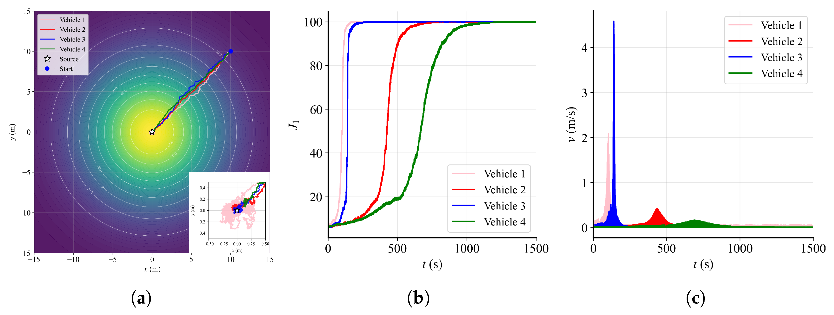
Different vehicles’ configurations and corresponding performance metrics are presented in Table 1 and Figure 4. All simulations were conducted in the same signal field as Simulation Experiment 1 with duration s.
Table 1.
Vehicle configurations and performance metrics.
Figure 4.
Simulation Experiment 2 result: (a) Trajectories of multiple vehicles. (b) as a function of time for each vehicle. (c) v as a function of time for each vehicle.
Figure 4 illustrates that all vehicles successfully accomplish source-seeking. Vehicle 1, with higher , achieves faster convergence ( s, ) but lower localization accuracy (final distance m) compared to Vehicle 2 ( m). Increasing k (Vehicle 2 vs. Vehicle 4) significantly accelerates convergence ( s vs. s; vs. ), while increasing (Vehicle 2 vs. Vehicle 3) similarly improves performance ( s → s; →).
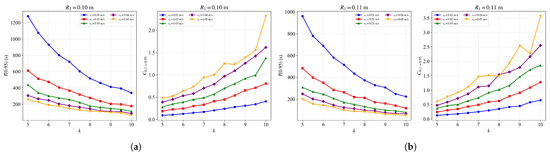
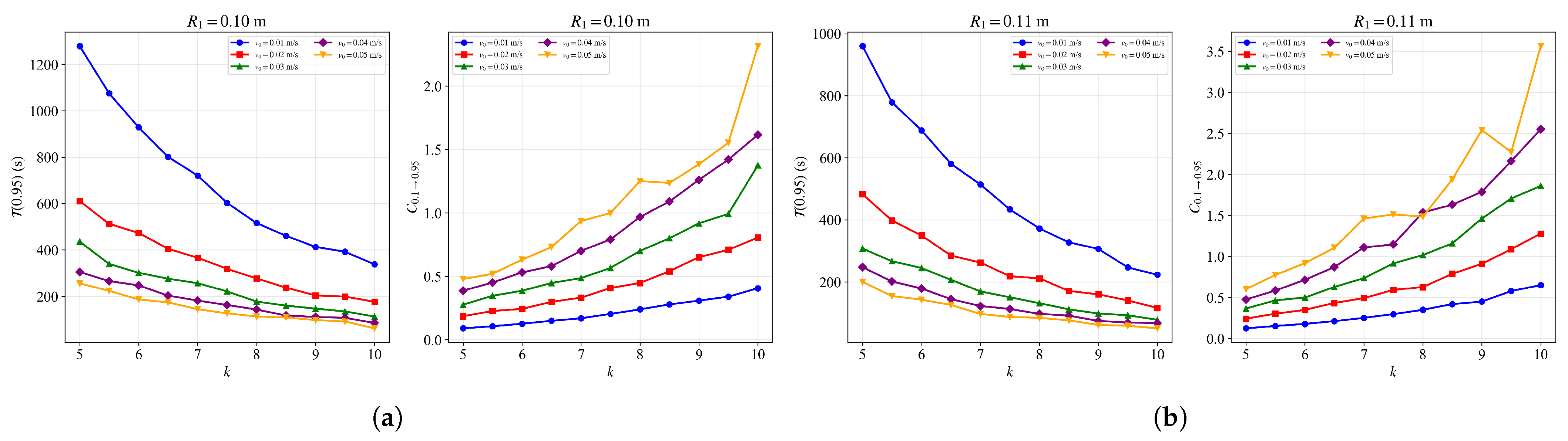
To further investigate the effects of these parameters, we performed a series of controlled experiments by varying k, (with held constant), and within the ranges specified in Table 2. The corresponding results are presented in Figure 5 and Figure A1 (see Appendix C).
Table 2.
Parameter scan ranges for sensitivity analysis.
Figure 5.
(a) and as functions of k for different , with m. (b) and as functions of k for different , with m.
Results illustrate that, with respect to , increasing the gain parameter k significantly reduces the time required for source localization when the initial velocity is small (approximately m/s). However, from the perspective of , the improvement achieved by increasing k is less pronounced for vehicles with a small initial velocity (approximately m/s) than for those with a larger initial velocity (approximately m/s). This is attributable to the fact that a small (e.g., m/s) creates a mobility bottleneck in the early stage. Increasing k amplifies weak gradient signals, enabling the vehicle to overcome this bottleneck and significantly reduce . However, since the vehicle’s speed remains fundamentally constrained by the low , the improvement in is limited.
In contrast, enlarging the sensor spacing leads to a steady improvement in both and . However, the magnitude of this improvement is less pronounced compared to the effects of varying k or . This is because a larger sensor spacing provides a stronger directional signal by amplifying the gradient measurement, which consistently enhances the vehicle’s ability to orient toward the source. Nevertheless, unlike k which directly amplifies the control response, or which fundamentally determines the baseline mobility, increasing only improves the quality of the sensory information without altering the vehicle’s inherent speed or control gain. Consequently, its impact on convergence performance is more gradual and less dramatic.
Based on the above analysis, we recommend the following parameter selection guidelines:
- For applications prioritizing convergence speed, a larger gain parameter k is recommended, particularly when the initial velocity is low.
- For applications prioritizing average convergence rate, a larger initial velocity combined with a moderate k yields the best improvement.
- Increasing the sensor spacing provides steady but gradual improvements in both metrics, serving as a complementary tuning parameter when finer adjustments are needed.
- A balanced configuration offers a good trade-off between convergence speed, average rate, and localization accuracy.
4.3. Simulation Experiment 3: Comparison with Other Algorithms
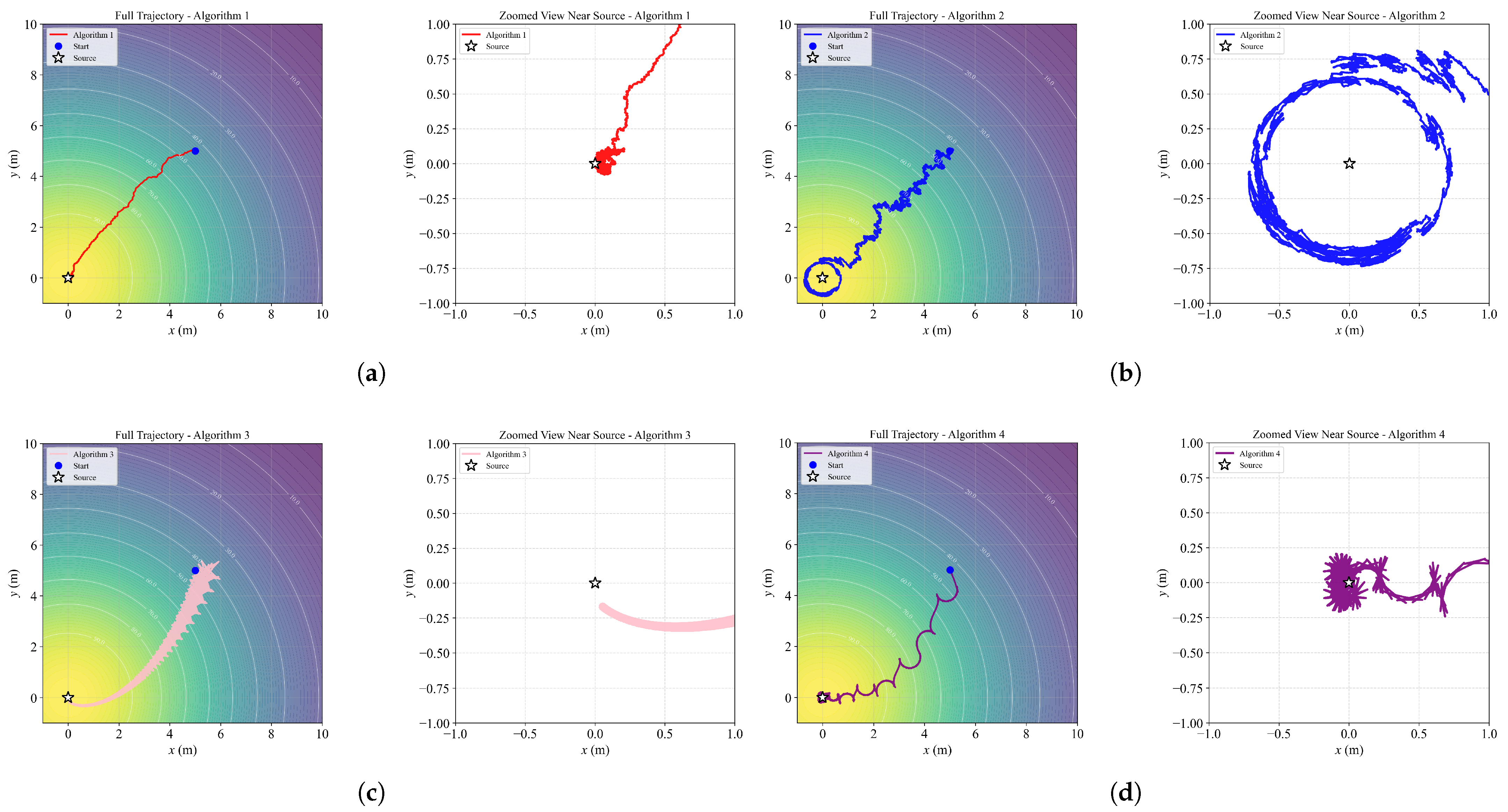
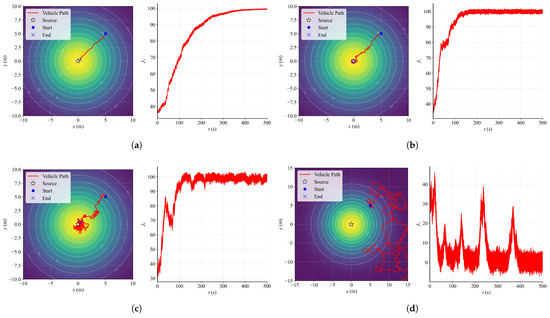
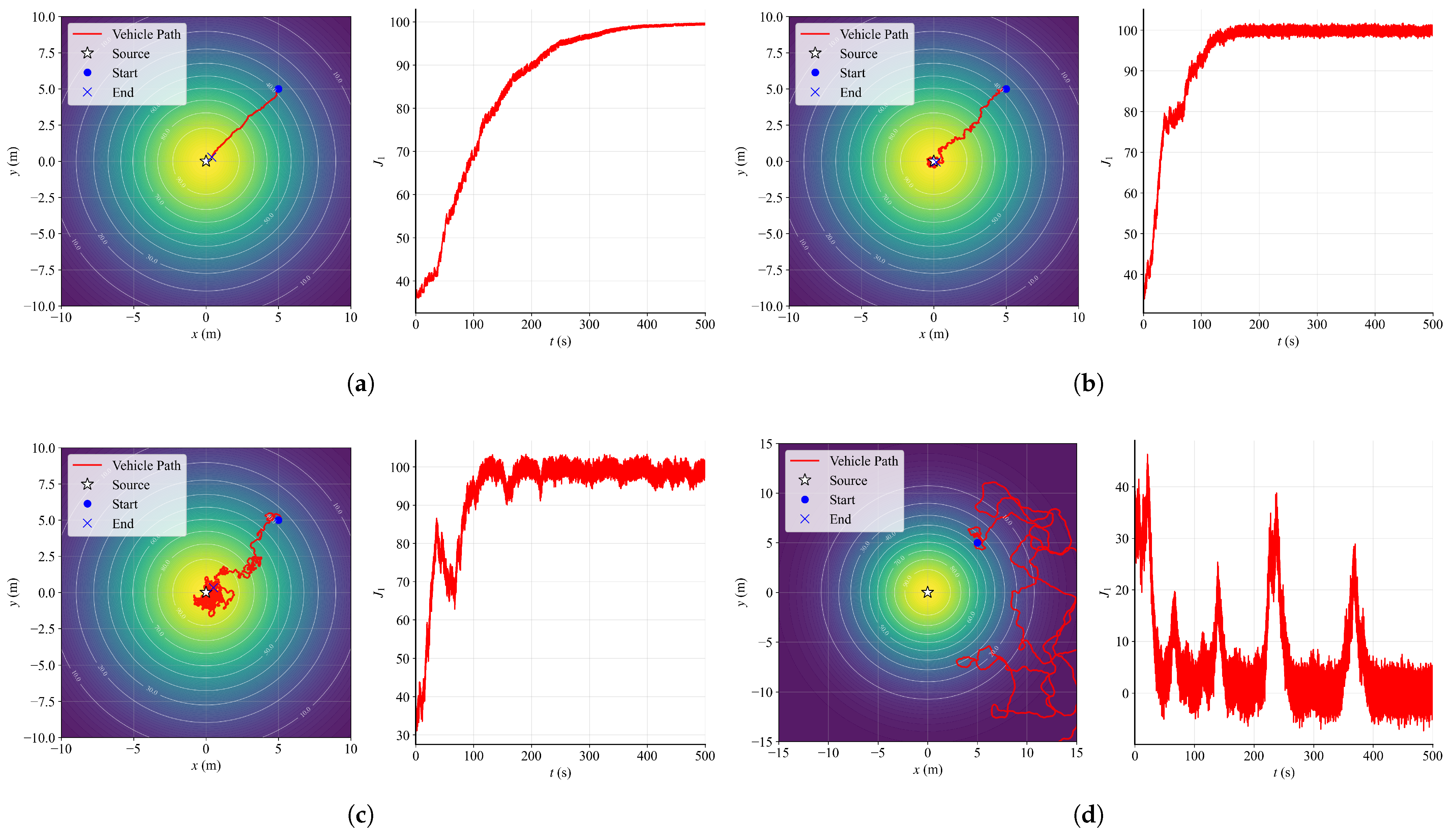
In this part, we focus on the differences in source-seeking behavior between our algorithm and other representative algorithms. We first set , , in Equation (1) and total simulation time s, then place all vehicles’ initial positions at . The parameter settings for each algorithm are shown in Table 3, and the simulation results are shown in Figure 6. This section offers a qualitative comparison of trajectory characteristics, focusing on observable differences in trajectory shapes and convergence behavior, as cross-algorithm performance is inherently sensitive to parameter tuning.
Table 3.
Parameter settings of each algorithm.
Figure 6.
Simulation Experiment 3 result: (a) Trajectory of our algorithm. (b) Trajectory of Algorithm 2 [16]. (c) Trajectory of Algorithm 3 [18]. (d) Trajectory of Algorithm 4 [29].
From Figure 6, qualitative differences in trajectory shape and characteristics can be observed among the algorithms. Our algorithm generates a trajectory with relatively direct and steady movement toward the source. Algorithm 2 produces a winding trajectory with an orbit-like path near the source. Algorithm 3 exhibits a pentagram-like trajectory pattern. Algorithm 4 follows a wave-like path. Additionally, periodic velocity reversals are observed during operation in Algorithms 3 and 4, while Algorithm 2 shows both positive and negative velocity variations at certain stages. These observed differences in trajectory patterns and velocity profiles highlight the distinct behavioral characteristics of each algorithm under the same experimental conditions.
4.4. Simulation Experiment 4: Performance in Complex Scenarios
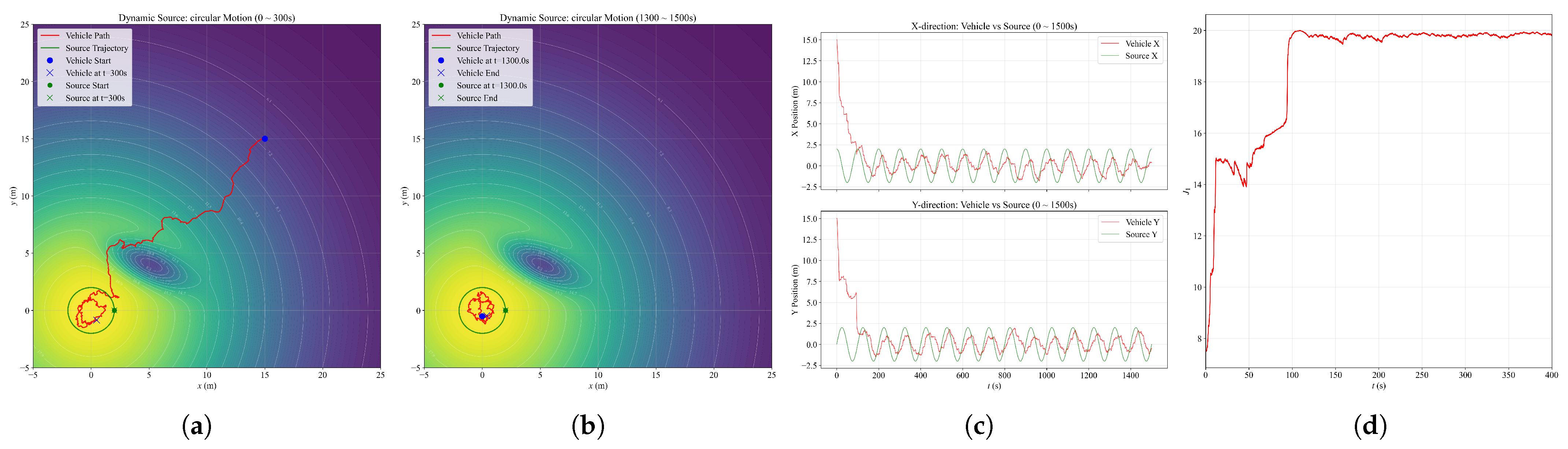
We constructed a signal field featuring a global maximum at the source location () and a local minimum in the surrounding region, forming a complex multi-modal landscape. The source moves according to a circular trajectory:
In this challenging environment, the vehicle must not only track the continuously moving source but also navigate carefully to avoid being trapped or repelled by the adjacent negative valley.
We initialize the vehicle at with m/s, m and m. The other parameters are , , , , . The total simulation duration is set to s. The simulation result is shown in Figure 7.
Figure 7.
Simulation Experiment 4 result: (a) Vehicle and source trajectories (first 300 s). (b) Vehicle and source trajectories (last 200 s). (c) Comparison of vehicle and source positions in X and Y directions over the full duration. (d) as a function of time (first 400 s).
As shown in Figure 7a, upon activation, the device initially moves rapidly toward the source along the radial direction. As it approaches a field trough, it turns rightward, gradually advancing along the gradient ascent direction while circumventing the trough. At approximately s, the device arrives in the vicinity of the source. Subsequently, as illustrated in Figure 7b,c, the source moves in a circular trajectory while the device follows, also tracing an approximately circular path around the source, maintaining stable motion in close proximity. These results demonstrate that the algorithm not only performs well in complex fields but also exhibits dynamic response characteristics when tracking a moving source.
4.5. Simulation Experiment 5: Robustness to Sensor Noise
To evaluate the robustness of the proposed algorithm against sensor imperfections, we inject additive Gaussian white noise into the sensor readings:
where denotes the standard deviation of the noise.
The signal field is configured with , , and . The vehicle parameters are set as , , , , , m/s, m, and m, with the initial position . Three sensor noise levels are considered: , 1, and 2, corresponding to approximately , , and of the source intensity , respectively, while serves as the noise-free baseline. Simulation results are shown in Figure 8 and Figure A2.
Figure 8.
Simulation Experiment 5 result: (a) . (b) . (c) . (d) .
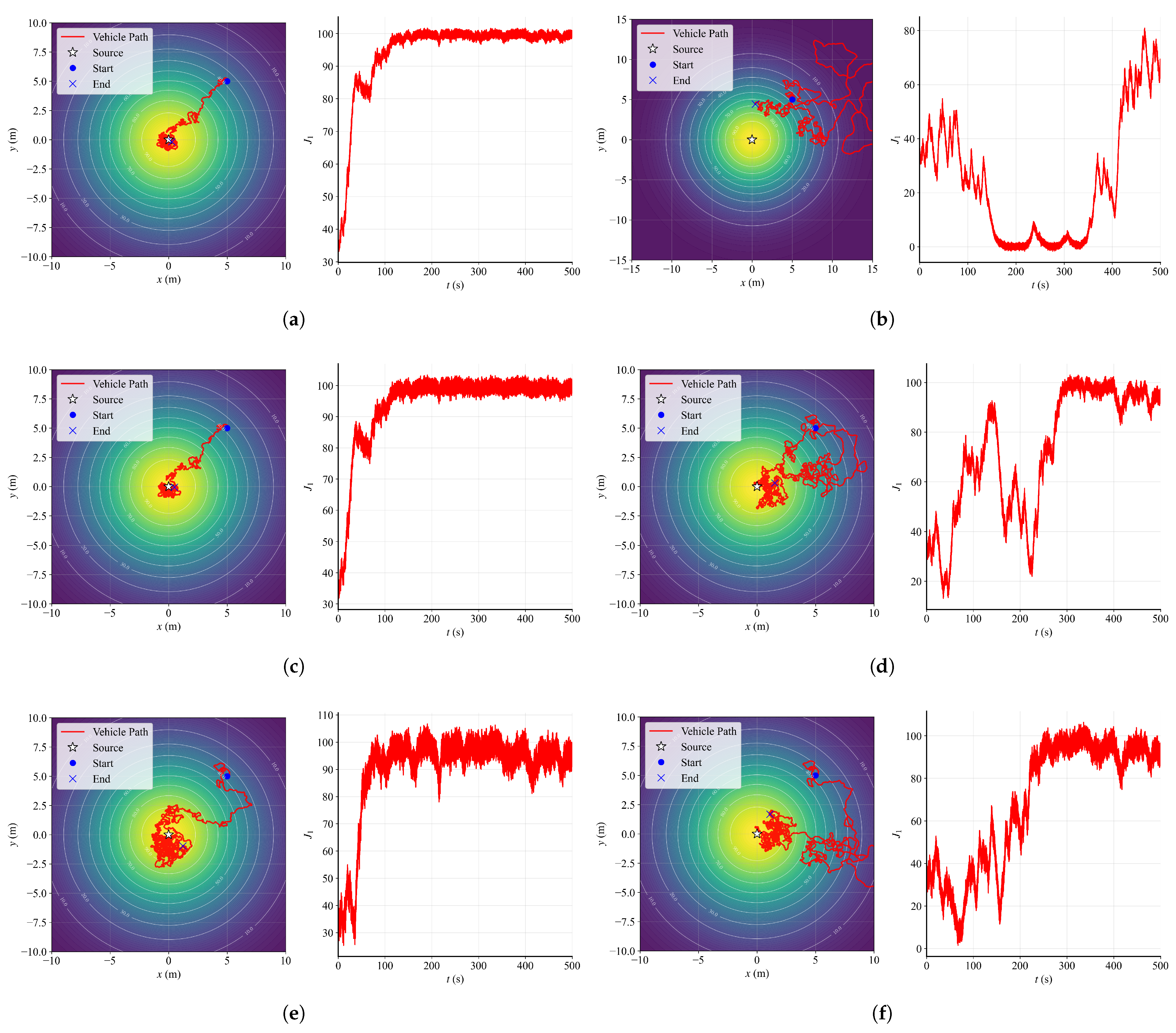
The experimental results reveal an asymmetry in the robustness of the two sensors: Sensor 2 exhibits significantly lower tolerance to noise compared to Sensor 1. Specifically, when , regardless of the noise level on Sensor 1 (illustrated by Figure 8d and Figure A2b,d), the vehicle either fails to locate the source entirely or exhibits severely degraded source-seeking performance. In contrast, increasing the noise on Sensor 1 only leads to a moderate degradation in localization accuracy and stability near the source, without causing complete mission failure. This asymmetry can be attributed to the fact that Sensor 1 is used in both the forward velocity regulation (together with Sensor 2) and the angular velocity control, whereas Sensor 2 is used exclusively for forward velocity regulation. Consequently, the control system is more sensitive to noise on Sensor 2, as it directly affects the velocity modulation that governs the vehicle’s approach to the source.
In addition, by comparing the trajectories in Figure 8a,b, we observe that an appropriate level of noise can, to some extent, reduce the convergence time from s to s. This counterintuitive phenomenon suggests that a moderate amount of sensor noise may introduce beneficial perturbations that help the vehicle escape local gradient traps or accelerate the exploration of the signal field, thereby improving convergence efficiency.
5. Physical Experiment
In the real-world experimental setup, a lamp was placed above the ground to serve as the signal emitter. A camera mounted directly above the emitter captured the real-time motion trajectory of the vehicle. No additional equipment was used to assist the vehicle in localization at any time.
5.1. Physical Experiment 1: Static Light Source
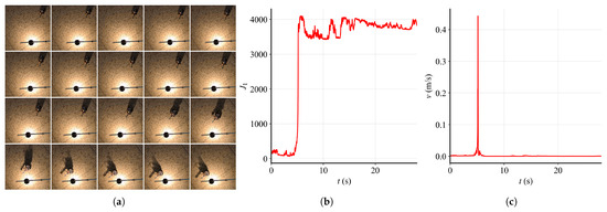
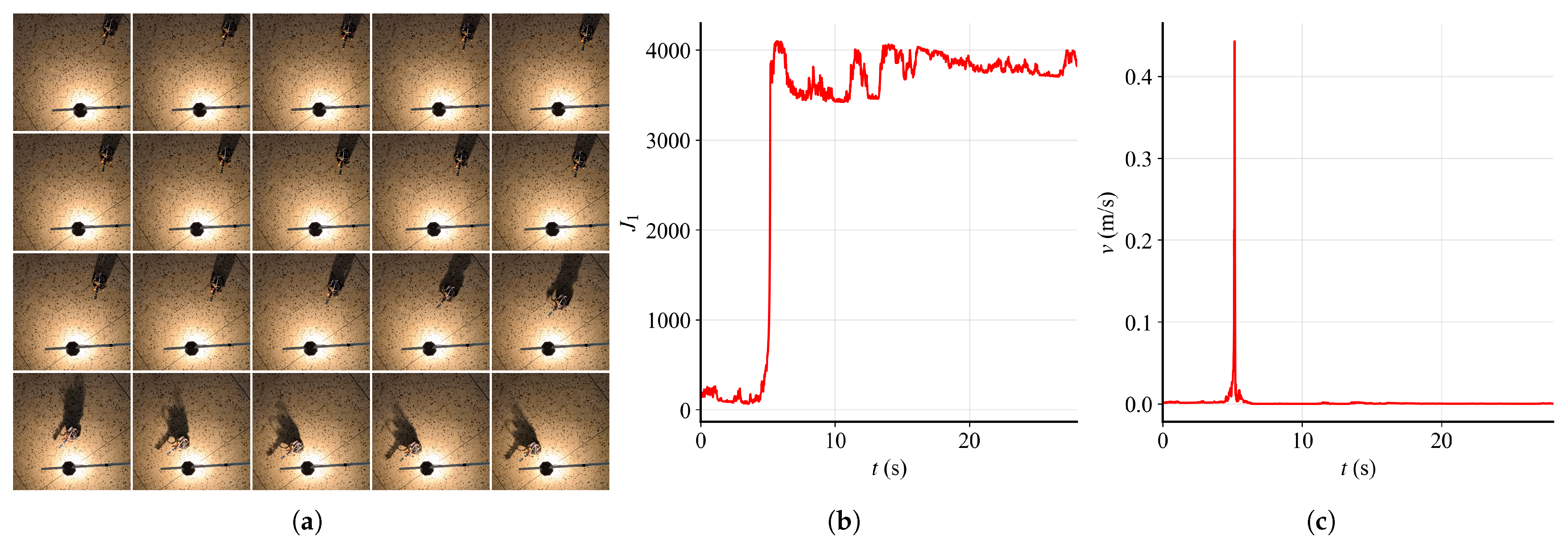
We placed the vehicle approximately 0.5 m away from the source, and the relevant parameters are configured as follows: m/s, , , , , . The trajectory of the vehicle with timestamp is shown in Figure 9 (pictures are extracted from Physical Experiment 1 (Overlook).mp4 in Supplementary Materials).
Figure 9.
Physical Experiment 1 result: (a) Physical experiment result with timestamp (time interval: 0.2 s). The center of the vehicle does not stop perfectly beneath the light source because the computing unit relies on analog signals when collecting measurements from the light-sensitive sensor. At the vehicle’s stationary position, the sensor reading reaches saturation (its maximum value), so the vehicle interprets that spot as the light source. (b) as a function of time. (c) v as a function of time.
As observed in Figure 9, the vehicle’s forward velocity evolves in several distinct phases after engagement. In the initial phase (0–2.4 s), the vehicle moves toward the source with a slowly increasing forward velocity. Subsequently, between 2.4 s and 3.0 s, the velocity increases sharply, allowing the vehicle to rapidly close in on the source. During the interval of 3.0–3.2 s, the velocity decreases. Beyond 3.2 s, the vehicle maintains stable motion in the vicinity of the source. After 3.8 s, although the forward velocity becomes extremely low, the angular velocity of the device remains actively driven by the algorithm, resulting in small-amplitude left-and-right oscillations. This phenomenon can be observed more clearly in Detailed Motion under Light Source.mp4 in Supplementary Materials.
Notably, the chosen is significantly smaller than its simulation counterpart (e.g., in Section 4.1). This difference arises because the physical sensors output raw ADC values (0–4095) with magnitudes far exceeding the normalized sensor readings in simulation. The lower gain is therefore necessary to prevent control saturation and maintain system stability in the presence of real-world sensor noise and hardware nonlinearities.
5.2. Physical Experiment 2: Flickering Light Source
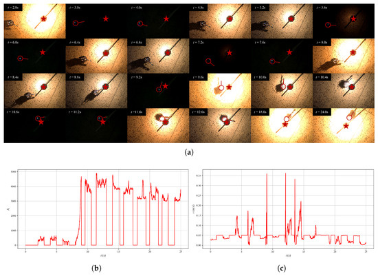
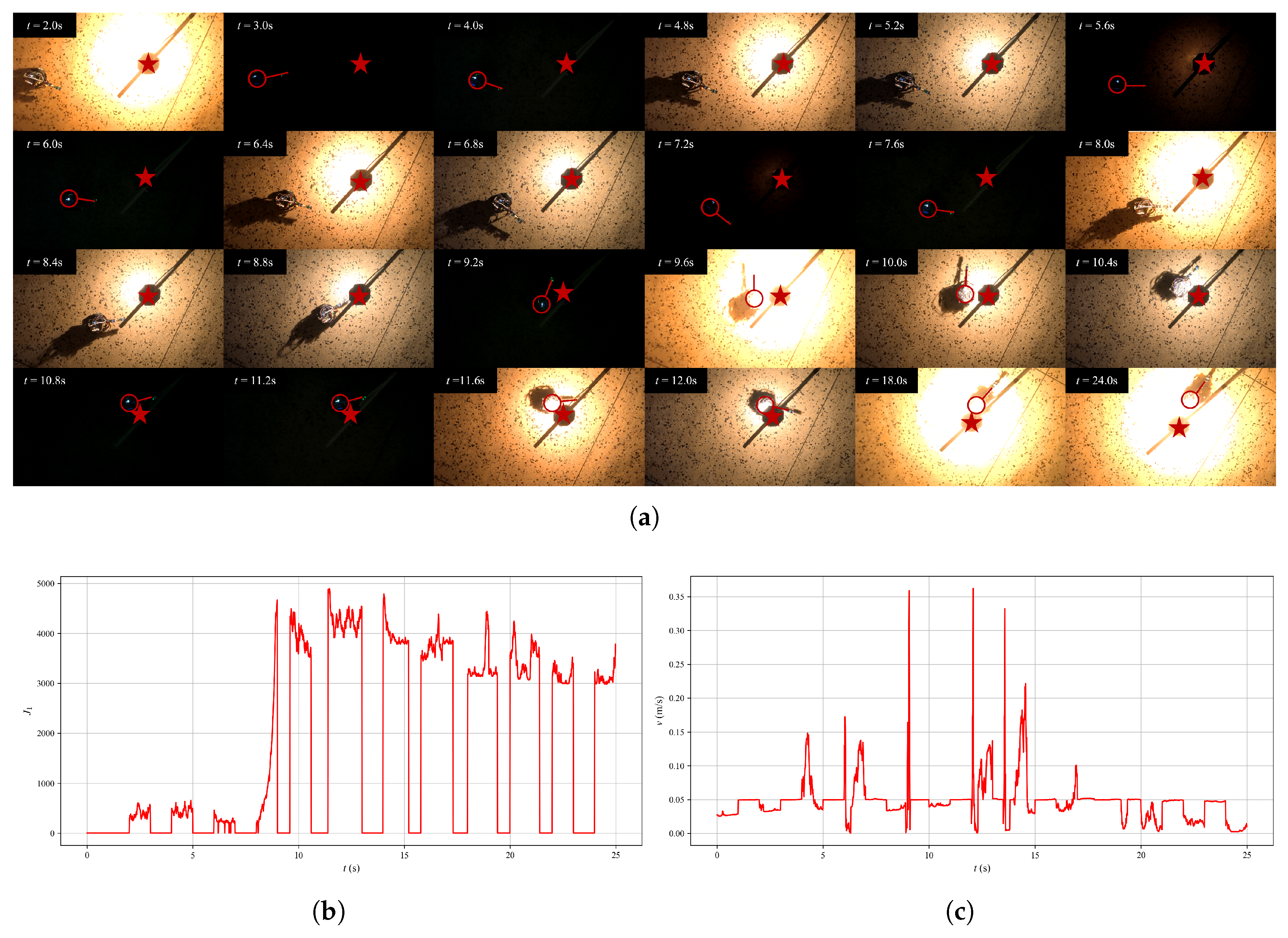
In this experiment, the light source intensity alternates between bright and dim states at a frequency of approximately 1 Hz, creating a flickering effect. We placed the vehicle approximately 0.5 m away from the source, and the relevant parameters are configured as follows: m/s, , , , , . The trajectory of the vehicle with timestamp is shown in Figure 10 (pictures are extracted from Physical Experiment 2 (Overlook).mp4 in Supplementary Materials).
Figure 10.
Physical Experiment 2 result: (a) Physical experiment result with timestamp.  denotes the source, while
 denotes the vehicle outline. (b) as a function of time. (c) v as a function of time.
denotes the source, while denotes the vehicle outline. (b) as a function of time. (c) v as a function of time.
As shown in Figure 10a, when the vehicle is in a dark environment, it swings while maintaining to explore the surrounding environment; when the vehicle is in a light environment, it adjusts its forward speed according to the sensor measurements and moves toward the light source. These two phenomena are particularly significant during the period of 8.0–12.0 s. At approximately 12.0 s, the vehicle moves to a position directly below the light source and remains near the source.
The behavior observed in both static and flickering scenarios aligns well with our simulation results, underscoring the practical engineering applicability of our algorithm.
6. Result
The results verify the proposed algorithm’s efficacy through simulations and real-world experiments. In simulations, the algorithm achieved fast convergence, consistently steering the agent to the source. Physical experiments under realistic conditions, including a static and a flickering light source, confirmed this performance, maintaining high localization accuracy. The strong quantitative agreement between the simulated and experimental outcomes underscores the algorithm’s robustness and its suitability for practical applications where environmental uncertainties are prevalent.
7. Discussion
While the simulation and physical experiments demonstrate the effectiveness of the proposed source-seeking approach, several limitations and open questions warrant further discussion.
- Partial sensor occlusion. In practical deployments, sensors may be partially occluded by obstacles, dust, water, or other parts of the robot. Because our angular velocity control exclusively relies on Sensor 1, occlusion of this sensor would cause complete failure of the source-seeking task. The current method lacks occlusion detection and sensor-switching fault tolerance. Systematic fault-tolerance tests and recovery mechanisms are deferred to future work.
- Multiple source interference. Real-world scenarios may contain multiple signal sources (e.g., multiple heat sources, chemical leak points, or electromagnetic emitters). Although our algorithm is designed to locate the strongest source, the vehicle may become trapped at a local maximum rather than the global peak, or oscillate between different sources in a multi-source environment (see more in Appendix E).
- Limitation to Three-Dimensional Environments. The current algorithm defines vehicle motion in the two-dimensional plane, with sensors mounted only along the vehicle’s longitudinal axis. This implicitly assumes that the signal field has no variation in the vertical direction (the z-axis) or that the vehicle is constrained to planar motion. However, in real three-dimensional scenarios such as cave systems, underwater canyons, multi-story buildings, or urban canyons, the source may be located at a different altitude, requiring the vehicle to adjust its pitch angle or depth to search for vertical gradients. Our current algorithm cannot extract such vertical gradient information, which may cause the vehicle to wander at an incorrect altitude without ever reaching the source.
- Empirical nature of convergence analysis. It should be emphasized that the convergence behavior reported in this paper is characterized based on experimental observations rather than rigorous mathematical proofs. While the simulation and physical results consistently demonstrate that the vehicle successfully converges to the vicinity of the light source under the proposed control strategy, a formal theoretical analysis—such as Lyapunov stability proof or asymptotic convergence guarantee—has not been established in the current study.
8. Conclusions
In this work, we proposed a source-seeking approach with angular and non-reversing forward velocity by using multi-sensor feedback. We not only examined our algorithm in simulation but also in physical experiments. The main contributions of this work are summarized as follows:
- In the model construction of the source-seeking device, we incorporate multiple sensors and design their layout structure to make the device capable of extracting spatial gradient information from the environmental field.
- We propose a novel forward velocity regulation method that distinguishes itself through the synergistic combination of multi-sensor fusion and nonlinear functions. Specifically, our approach leverages the inherent properties of two key functions: the hyperbolic tangent for its bounded output to cap the maximum speed, and the exponential function for its continuous and non-negative nature to guarantee smooth and strictly positive velocity commands. This combination allows for a more nuanced and physically realizable control compared to conventional techniques.
- Based on those mentioned above, we conducted systematic simulation experiments to observe the impact of different parameter values on the experimental results. This will facilitate future researchers adopting the same concept to further consider establishing a theoretical model for the relationship between sensor spacing, convergence speed, and localization accuracy, thereby contributing to the development of more efficient and higher-precision source-seeking algorithms.
- Finally, the successful validation of our algorithm on the real-world TWDDR platform strongly supports our core claim that the proposed method is both efficient and robust for this type of task.
While the current work primarily focuses on sensor configuration optimization for a single source-seeking device, we will extend this concept to multi-agent systems in future work. We plan to investigate how to further improve the information collection efficiency and localization accuracy of the swarm by optimizing the relative positions and sensor configurations among multiple agents during cooperative source-seeking. In addition, for single-device scenarios, we will explore alternative sensor arrangements beyond collinear placement (e.g., non-collinear or multi-directional configurations) to enhance spatial gradient estimation.
Supplementary Materials
The following supporting information can be downloaded at: https://www.mdpi.com/article/10.3390/math14132260/s1, Detailed Motion under Light Source.mp4; Physical Experiment 1 (Overlook).mp4; Physical Experiment 2 (Overlook).mp4.
Author Contributions
Conceptualization, Q.S. and J.S.; methodology, Q.S. and G.L.; software, Q.S. and G.L.; validation, Q.S., G.L., J.S. and R.W.; writing—original draft preparation, Q.S. and J.S.; writing—review and editing, W.Z. and M.G. All authors have read and agreed to the published version of the manuscript.
Funding
This research received no external funding.
Data Availability Statement
The original contributions presented in this study are included in the article. The materials, photographs, and experimental videos of TWDDR and Physical Experiment are publicly available at: https://github.com/Autonomous-Source-Seeking-Team-ASST/Source-Seeking-Approach-with-Non-Reversing-Forward-Velocity-Regulation-via-Multi-Sensor-Feedback (accessed on 20 June 2026). In the event that the link is no longer accessible (e.g., due to force majeure), the corresponding author may be contacted to provide these materials upon reasonable request.
Acknowledgments
The authors would like to express their sincere gratitude to the Open Hardware Association Club of Sichuan University (https://bbs.scumaker.org (accessed on 20 June 2026)) for providing hardware materials and venue resources in support of this work. During the preparation of this work, the authors used DeepSeek (web version, DeepSeek-V3; available at https://www.deepseek.com/, accessed on 20 June 2026) for language polishing and Doubao (web version, Doubao-Seed-2.0; available at https://www.doubao.com/chat/, accessed on 20 June 2026) for minor image processing of Figure 1a,b (brightness adjustment and background removal only). The authors have reviewed and take full responsibility for all content.
Conflicts of Interest
The authors declare no conflicts of interest.
Appendix A. Robot Kinematic Equations
Let the left and right wheel linear velocities be and , and the wheelbase (distance between the two wheels) be L. Then the linear velocity v and angular velocity at the robot’s center point are given by:
And the pose update differential kinematic equations are:
Appendix B. Details About Vehicle’s Hardware
This appendix presents the hardware components of the TWDDR used in our experiments.
Table A1.
List of components used in the TWDDR platform.
Appendix C. Sensitivity Analysis of Key Parameters
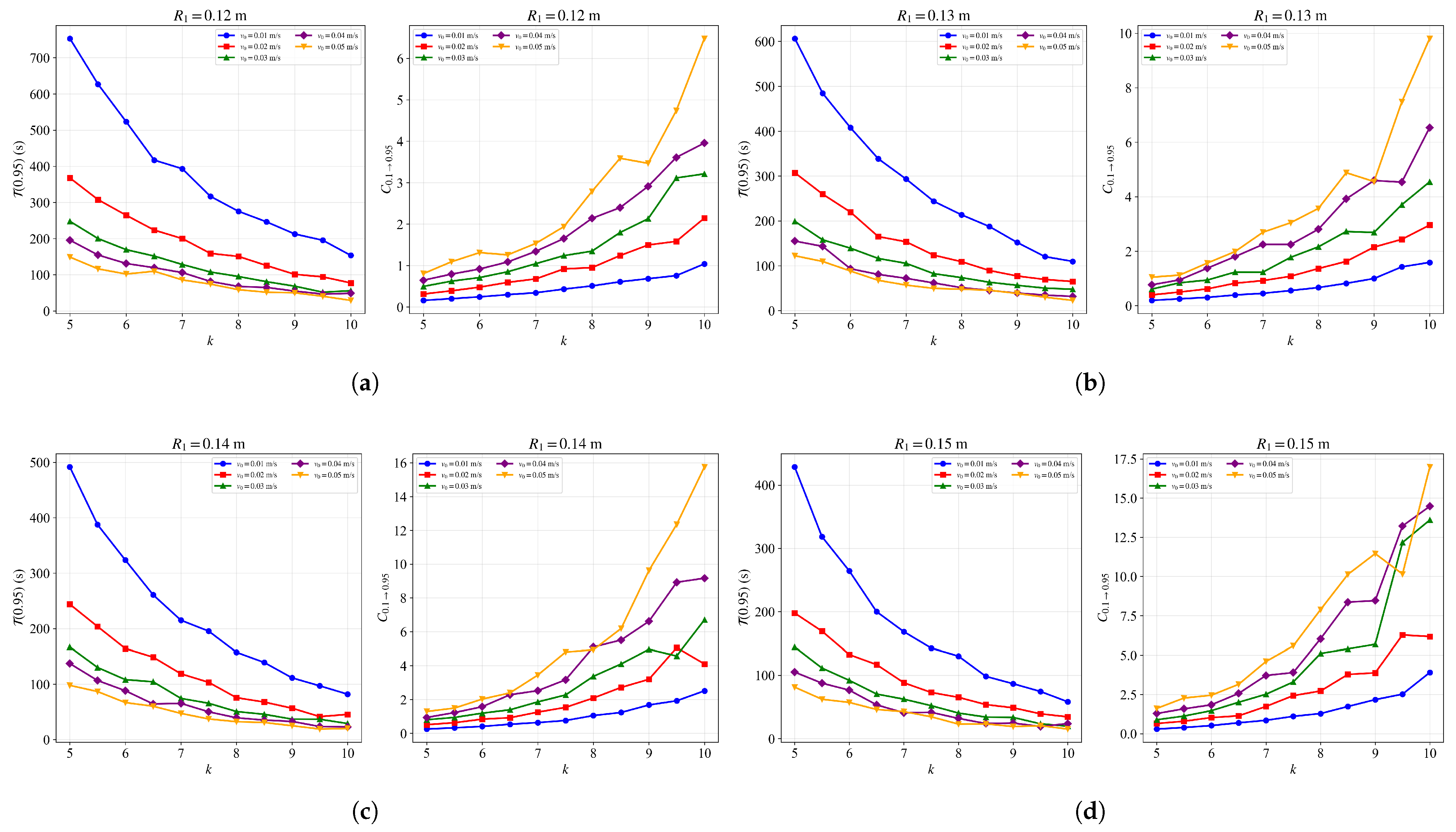
This appendix provides additional simulation results examining the sensitivity of the source-seeking algorithm to three key parameters: k, , and .
Figure A1.
(a) and as functions of k for different , with m. (b) and as functions of k for different , with m. (c) and as functions of k for different , with m. (d) and as functions of k for different , with m.
Appendix D. Supplementary Figures of Sensor Noise Robustness
This section presents supplementary figures for the sensor noise robustness experiments.
Figure A2.
Simulation Experiment 5 results under different sensor noise combinations: (a) , . (b) , . (c) , . (d) , . (e) , . (f) , .
Appendix E. Performance in Multiple Source Environment
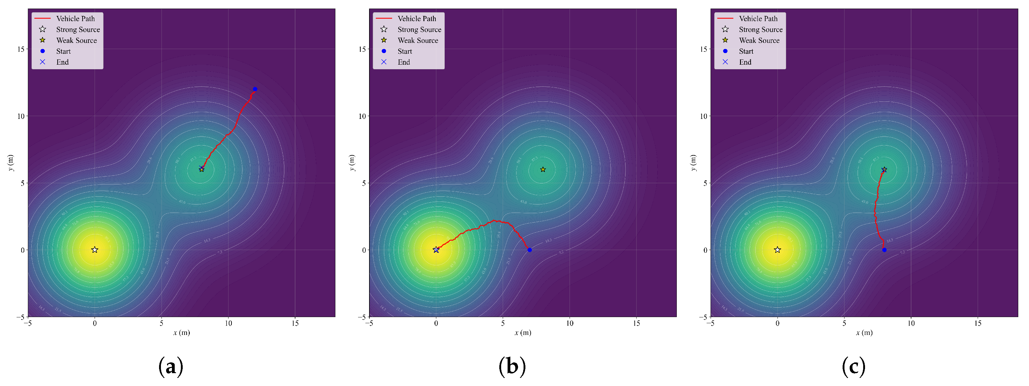
This appendix presents the results of the multi-source experiment mentioned in Section 7. The experimental setup includes two signal sources with different intensities, simulating an environment where multiple peaks coexist.
Figure A3 indicates that the proposed algorithm does not guarantee global convergence in multi-source environments, and the outcome depends on the initial position. Addressing such scenarios would require the introduction of multi-peak search or source separation mechanisms in future work.
Figure A3.
Vehicle trajectories in a multi-source environment. (a) Starting from . (b) Starting from . (c) Starting from .
References
- Talwar, D.; Lu, T.; Sobti, D.; Wu, W. Multi-Robot Source Seeking and Field Reconstruction of Spatial-Temporal Varying Fields. In Proceedings of the 2024 9th International Conference on Automation, Control and Robotics Engineering (CACRE); IEEE: Jeju Island, Republic of Korea, 2024; pp. 101–105. [Google Scholar]
- Xu, S.; Wang, Y.; Xu, D.; Zhu, X.; Chen, H. A Review on Source Seeking Control and Its Application to Wheeled Mobile Robots. In Proceedings of the 2019 3rd Conference on Vehicle Control and Intelligence (CVCI); IEEE: Hefei, China, 2019; pp. 1–5. [Google Scholar]
- Du, B.; Qian, K.; Claudel, C.; Sun, D. Multi-Agent Online Source Seeking Against Non-Stochastic Disturbances. IEEE Trans. Autom. Control 2026, 71, 4097–4104. [Google Scholar] [CrossRef] [Scilit]
- Fabbiano, R.; Garin, F.; Canudas-de Wit, C. Distributed Source Seeking Without Global Position Information. IEEE Trans. Control Netw. Syst. 2018, 5, 228–238. [Google Scholar]
- Li, Z.; You, K.; Song, S. AUV Based Source Seeking with Estimated Gradients. J. Syst. Sci. Complex. 2018, 31, 262–275. [Google Scholar] [CrossRef] [Scilit]
- Zhang, T.; Qin, V.; Tang, Y.; Li, N. Distributed Information-Based Source Seeking. IEEE Trans. Robot. 2023, 39, 4749–4767. [Google Scholar] [CrossRef] [Scilit]
- Fu, L.; Ozguner, U. Extremum-Seeking Control in Constrained Source Tracing With Nonholonomic Vehicles. IEEE Trans. Ind. Electron. 2009, 56, 3602–3608. [Google Scholar] [CrossRef] [Scilit]
- Ghadiri-Modarres, M.; Mojiri, M.; Fattahi, E. Multi-Agent Deployment Around a Source in the Plane Using Biased Extremum Seeking. In Proceedings of the 2021 29th Iranian Conference on Electrical Engineering (ICEE); IEEE: Tehran, Iran, 2021; pp. 649–653. [Google Scholar]
- Ghadiri-Modarres, M.; Mojiri, M. Normalized Extremum Seeking and Its Application to Nonholonomic Source Localization. IEEE Trans. Autom. Control 2021, 66, 2281–2288. [Google Scholar] [CrossRef] [Scilit]
- Jabeen, M.; Meng, Q.H.; Jin, L.C.; Jin, S.; Deng, Z.Y. Adaptive-extremum seeking control algorithm to seek the odor source using a multi-agent system. In Proceedings of the 2022 41st Chinese Control Conference (CCC); IEEE: Hefei, China, 2022; pp. 4678–4683. [Google Scholar]
- Liu, S.J.; Krstic, M. Stochastic source seeking for nonholonomic unicycle. Automatica 2010, 46, 1443–1453. [Google Scholar] [CrossRef] [Scilit]
- Cochran, J.; Siranosian, A.; Ghods, N.; Arnold, D.; Krstic, M. GPS-denied source seeking for a nonholonomic unicycle via heading control. IFAC Proc. Vol. 2007, 40, 952–957. [Google Scholar] [CrossRef] [Scilit]
- Eqab, H.; Salamah, Y.B.; Ahmad, I.; Morsy, M.A. Development of source seeking algorithm for mobile robots. Intell. Serv. Robot. 2023, 16, 393–401. [Google Scholar] [CrossRef] [Scilit]
- Sun, Q.; Shen, J.; Li, G. Adaptive-Excitation Stochastic Source Seeking for Two-Wheeled Differential Drive Robot. In Proceedings of the 2026 12th International Conference on Control, Automation and Robotics (ICCAR); IEEE: Nagoya, Japan, 2026; pp. 17–25. [Google Scholar]
- Zhuo, S.; Li, C.; Chen, S. Source seeking of UAV via adaptive extremum seeking without steady-state oscillation. In Proceedings of the 2017 IEEE International Conference on Unmanned Systems (ICUS); IEEE: Beijing, China, 2017; pp. 61–65. [Google Scholar]
- Lin, J.; Song, S.; You, K.; Krstic, M. Stochastic source seeking with forward and angular velocity regulation. Automatica 2017, 83, 378–386. [Google Scholar] [CrossRef] [Scilit]
- Xu, T.; Chen, G.; Zhou, G.; Liu, Z.; Zhang, Z.; Yuan, S. Fast Source Seeking with Obstacle Avoidance via Extremum Seeking Control. In Proceedings of the 2022 13th Asian Control Conference (ASCC); IEEE: Jeju Island, Korea, 2022; pp. 2097–2102. [Google Scholar]
- Elgohary, A.A.; Eisa, S.A.; Bajpai, S. Model-Free and Real-Time Unicycle-Based Source Seeking with Differential Wheeled Robotic Experiments. IFAC-PapersOnLine 2025, 59, 25–30. [Google Scholar] [CrossRef] [Scilit]
- Palanikumar, R.; Elgohary, A.A.; Grushkovskaya, V.; Eisa, S.A. Model-free source seeking of exponentially convergent unicycle: Theoretical and robotic experimental results. IFAC J. Syst. Control 2026, 35, 100378. [Google Scholar] [CrossRef] [Scilit]
- Lin, J.; You, K.; Song, S. Velocity regulation in 3D nonholonomic source seeking. In Proceedings of the 11th World Congress on Intelligent Control and Automation; IEEE: Shengyang, China, 2014; pp. 1112–1117. [Google Scholar]
- Qian, H.; Wang, M.; Zhu, M.; Wang, H. A Review of Multi-Sensor Fusion in Autonomous Driving. Sensors 2025, 25, 6033. [Google Scholar] [CrossRef] [Scilit] [PubMed]
- Osman, A.; Shamsfakhr, F.; Vecchio, M.; Antonelli, F. Adaptive GNSS–UWB sensor fusion for reliable localization in precision agriculture. Smart Agric. Technol. 2026, 13, 101846. [Google Scholar] [CrossRef] [Scilit]
- Zhang, P.; Yang, L.; Liu, S.J. Distributed stochastic source seeking and formation control based on delayed measurements. Sci. China Inf. Sci. 2025, 68, 132208. [Google Scholar] [CrossRef] [Scilit]
- Sorge, M.; Cigarini, N.; Lorigiola, R.; Michieletto, G.; Masiero, A.; Cenedese, A.; Guarnieri, A. Multi Agent Switching Mode Controller for Sound Source Localization. IFAC-PapersOnLine 2025, 59, 167–172. [Google Scholar] [CrossRef] [Scilit]
- Wang, H.; Li, H.; Zou, H.; Chi, H.; Lan, L.; Huang, W.; Yang, W. Effective and efficient time-varying counterfactual prediction with state-space models. In Proceedings of the Thirteenth International Conference on Learning Representations, Singapore, 24–28 April 2025. [Google Scholar]
- Wang, H.; Yang, W.; Yang, L.; Wu, A.; Xu, L.; Ren, J.; Wu, F.; Kuang, K. Estimating individualized causal effect with confounded instruments. In Proceedings of the 28th ACM SIGKDD Conference on Knowledge Discovery and Data Mining; ACM: New York, NY, USA, 2022; pp. 1857–1867. [Google Scholar]
- Wang, H.; Kuang, K.; Lan, L.; Wang, Z.; Huang, W.; Wu, F.; Yang, W. Out-of-distribution generalization with causal feature separation. IEEE Trans. Knowl. Data Eng. 2023, 36, 1758–1772. [Google Scholar] [CrossRef] [Scilit]
- Wang, H.; Zou, H.; Li, H.; Chi, H.; Shi, Y.; Zhang, Y.; Yang, W.; Liu, X.; Lin, Z. Transformers with Endogenous In-Context Learning: Bias Characterization and Mitigation. In Proceedings of the Fourteenth International Conference on Learning Representations, Rio de Janeiro, Brazil, 23–27 April 2026. [Google Scholar]
- Suttner, R.; Krstić, M. Acceleration-Actuated Source Seeking Without Position and Velocity Sensing. IFAC-PapersOnLine 2020, 53, 5348–5355. [Google Scholar] [CrossRef] [Scilit]

Disclaimer/Publisher’s Note: The statements, opinions and data contained in all publications are solely those of the individual author(s) and contributor(s) and not of MDPI and/or the editor(s). MDPI and/or the editor(s) disclaim responsibility for any injury to people or property resulting from any ideas, methods, instructions or products referred to in the content. |
© 2026 by the authors. Licensee MDPI, Basel, Switzerland. This article is an open access article distributed under the terms and conditions of the Creative Commons Attribution (CC BY) license.