


Abstract
Heat transport in heterogeneous materials can deviate markedly from classical Fourier behavior when microstructural disorder, trapping effects, nonlinear mobility, and long-range temporal correlations interact across multiple spatial and temporal scales. These mechanisms may produce delayed relaxation, persistent thermal footprints, front deformation, and non-classical spreading patterns that are not adequately represented by conventional integer-order diffusion models. In this study, a modeling and simulation framework is developed for anomalous heat transport in heterogeneous media using a two-dimensional time-fractional porous medium equation. The model combines a Caputo fractional time derivative, which represents thermal memory, with nonlinear degenerate porous-medium diffusion, spatially heterogeneous conductivity, localized volumetric heating, and Robin-type convective boundary exchange. A conservative fully discrete numerical scheme is constructed using flux-based finite differences for the heterogeneous nonlinear diffusion operator and an approximation for the Caputo derivative. The nonlinear algebraic system at each time level is solved using an under-relaxed Picard frozen-coefficient iteration with non-negativity enforcement and sparse direct solution of the resulting linear systems. The numerical implementation is verified through a manufactured-solution convergence study, and additional analyses are performed to examine computational cost, Picard iteration behavior, coefficient-regularization sensitivity, strong-source effects, heterogeneous conductivity structures, and long-time thermal-footprint persistence. The results show that heterogeneous conductivity mainly redirects heat through preferential pathways and enlarges the spatial footprint while producing negligible changes in global heat content. Stronger fractional memory, represented by smaller fractional order, increases the persistence and spatial reach of moderate heating, whereas larger porous-medium exponents confine heat near the source and preserve higher local peaks. Source amplitude increases the thermal burden and footprint monotonically over the tested range, including strong forcing, without producing an abrupt localization-spreading transition. Boundary exchange remains secondary in the short-time interior-heating regime considered. These findings demonstrate that the proposed two-dimensional time-fractional porous medium framework provides a verified and physically interpretable model for non-Fourier heat transport in heterogeneous materials, where local intensity, global heat retention, and spatial thermal exposure must be assessed jointly.
Keywords:
anomalous heat transport; thermal memory effects; porous and composite materials; time-fractional MSC:
74A15; 34A08; 34K37; 65L80
1. Introduction
Heat transport is a fundamental process in condensed matter physics, materials science, geophysics, energy engineering, and thermal management systems [1,2]. In classical theory, heat conduction is commonly described by Fourier’s law, which leads to a parabolic diffusion equation characterized by instantaneous propagation of thermal disturbances and exponential relaxation [3]. Although this framework is effective for homogeneous and well-ordered materials, many porous solids, composites, granular media, layered structures, microstructured materials, and nanostructured systems exhibit delayed propagation, non-Gaussian spreading, and persistent thermal localization that cannot be fully represented by conventional Fourier-based models [1,2,4]. In this context, non-Fourier transport should be understood as a broad deviation from classical heat conduction, arising from mechanisms such as memory-dependent relaxation, anomalous temporal scaling, nonlinear mobility, and spatially heterogeneous conduction pathways.
These nonclassical transport responses are often induced by microstructural disorder, trapping and release processes, tortuous conduction routes, heterogeneous interfaces, and sustained temporal correlations [4,5,6]. Such effects may generate delayed thermal fronts, long-lived hot regions, and power-law-type relaxation instead of the exponential decay expected from classical diffusion [1,2,6]. Fractional calculus provides a natural way to incorporate these memory effects into transport models, since time-fractional derivatives allow the present thermal state to depend on the accumulated history of the system [7,8,9]. At the same time, porous-medium and nonlinear diffusion models describe state-dependent mobility, degenerate diffusion, localization, and finite-speed-type spreading, which are relevant when heat transport depends on the local thermal state or becomes suppressed near ambient conditions [3,7,9]. Thus, fractional memory and porous-medium degeneracy represent distinct but complementary mechanisms: the former modifies temporal relaxation through a history kernel, whereas the latter modifies spatial transport through nonlinear mobility.
Combining these mechanisms within a two-dimensional time-fractional porous medium equation provides a physically interpretable route for modeling anomalous heat transport in heterogeneous materials. In this framework, the Caputo fractional derivative represents thermal memory, the porous-medium diffusion term captures nonlinear mobility and localization, and the spatially varying conductivity field represents heterogeneous heat pathways. When localized volumetric heating and convective boundary exchange are also included, the model can describe situations in which heat propagation is governed simultaneously by memory, nonlinearity, material heterogeneity, source intensity, and environmental exchange. This integrated structure is important because these mechanisms do not necessarily affect the same observable quantity: memory may increase persistence, nonlinear mobility may confine or sharpen thermal fronts, and heterogeneity may redistribute heat spatially without strongly changing the total heat content.
Despite its modeling relevance, the numerical simulation of the two-dimensional time-fractional porous medium equation remains challenging. The Caputo derivative introduces nonlocal temporal coupling, which increases memory requirements and computational cost [8,10,11]. The nonlinear porous-medium term can become degenerate near low-temperature regions, which complicates stability, convergence, and positivity preservation [9,12]. These difficulties are amplified in heterogeneous two-dimensional domains, where the spatial discretization must preserve the conservative flux structure while accounting for variable conductivity, nonlinear mobility, localized forcing, and Robin-type boundary exchange. Existing studies often address linear fractional diffusion, one-dimensional problems, simplified coefficients, or idealized boundary conditions [8,10,13], whereas many physically motivated heat-transport models emphasize anomalous behavior without connecting the model, numerical implementation, verification, and diagnostic interpretation in a unified framework [3,6,14,15].
Furthermore, previous modeling and numerical studies have examined important components of fractional heat transport, including time-fractional porous-medium dynamics, anomalous diffusion, self-similar behavior, compactly supported solutions, and convergent numerical schemes [12,16,17]. Other works have considered fractional heat conduction in porous or fractured media, often with benchmark as well as fractional diffusion and reaction-diffusion problems with Robin boundary conditions to clarify memory effects, boundary exchange, comparison principles, and finite-difference accuracy [18,19,20,21]. However, these contributions generally address isolated aspects of the problem, such as one-dimensional porous-medium flow, linear fractional conduction, homogeneous media, idealized boundary conditions, or mainly analytical properties. The present study advances this literature by integrating Caputo thermal memory, nonlinear degenerate porous-medium diffusion, spatially heterogeneous conductivity, localized heat generation, and Robin-type convective exchange within a verified two-dimensional numerical framework. This formulation enables the coupled roles of memory, nonlinear mobility, heterogeneity, source intensity, and boundary exchange to be assessed through physically interpretable diagnostics, including peak temperature, total heat content, and thermal footprint.
Motivated by these gaps, this study develops a modeling and simulation framework for memory-driven anomalous heat transport governed by a two-dimensional time-fractional porous medium equation. The model incorporates a Caputo fractional time derivative, nonlinear porous-medium diffusion, spatially heterogeneous conductivity, localized volumetric heating, and convective boundary exchange. The numerical scheme combines a conservative flux-based finite difference discretization, an L1 approximation of the Caputo derivative, semi-implicit Picard linearization, under-relaxation, non-negativity enforcement, and sparse direct solution of the resulting algebraic systems. The numerical framework is further assessed through manufactured-solution verification, grid-refinement analysis, coefficient-regularization sensitivity, computational-cost evaluation, and parameter studies that separate the effects of fractional memory, nonlinear mobility, heterogeneity, source amplitude, and boundary exchange.
The main contribution of this study is therefore threefold. First, it formulates a physically interpretable two-dimensional heat-transport model that combines Caputo memory, porous-medium mobility, heterogeneous conductivity, localized heating, and Robin boundary exchange within a single continuum framework. Second, it provides an implementation-faithful numerical strategy that preserves the conservative flux structure while addressing nonlinearity, memory, positivity, and reproducibility. Third, it interprets anomalous heat transport through complementary diagnostics, including peak temperature, total heat content, and thermal footprint, thereby distinguishing local hot-spot intensity, global heat retention, and spatial thermal exposure. The novelty does not lie in the isolated use of an L1 approximation or Picard iteration, since these are established numerical tools. Rather, it lies in their integration with heterogeneous nonlinear heat transport, positivity-aware implementation, verification, and mechanism-oriented diagnostics within a single two-dimensional framework. This enables the study to clarify how memory, nonlinear mobility, and heterogeneity interact to produce delayed relaxation, preferential heat redistribution, persistent thermal footprints, and localization-spreading transitions.
2. Mathematical Model Formulation for Anomalous Heat Transport
2.1. Physical Context and Modeling Rationale
Heat transport in heterogeneous solids can depart significantly from the predictions of classical Fourier theory. In porous ceramics, composites, rocks, and engineered microstructured materials, thermal energy does not move through a uniform continuum. Instead, heat carriers undergo repeated trapping and delayed release, and they migrate through tortuous conduction networks shaped by pores, grain boundaries, inclusions, and multiscale disorder. When these microscopic mechanisms accumulate across length scales, the macroscopic response often exhibits delayed thermal fronts, persistent hot regions, non-Gaussian spreading, and relaxation behaviors that are not well described by a single exponential timescale [22,23,24].
A significant implication of these observations is that the instantaneous heat flux cannot be determined solely by the local temperature gradient at that moment. Rather, the observed evolution reflects the cumulative thermal history of the material, which is naturally captured by fractional time operators. Time-fractional derivatives introduce a power-law memory kernel that provides a compact and physically consistent description of long-range temporal correlations induced by trapping, heterogeneous microstructure, and delayed energy exchange [25,26,27]. Importantly, this memory mechanism can be incorporated without introducing auxiliary internal variables whose calibration may be ambiguous.
Memory, however, is only one part of a realistic model. In many heterogeneous solids the effective conductivity varies in space, and it can also depend on temperature because conduction pathways become activated as the thermal state changes. In addition, experiments frequently involve Localized volumetric heating (for example laser irradiation, Joule heating, or exothermic reactions) together with heat exchange with the surrounding environment. A useful continuum description should therefore combine thermal storage with memory, nonlinear and heterogeneous conduction, internal heat generation, and boundary exchange. These ingredients are naturally unified within a time-fractional porous medium framework [3,14].
2.2. Dimensional Energy Balance and Constitutive Assumptions
Let be the dimensional temperature (K) in a bounded domain , and let denote the ambient reference temperature. A macroscopic energy balance incorporating memory in the thermal storage mechanism is written as
where is the Caputo order, is density, is specific heat, is an effective conductivity, and Q is a volumetric heat source (W m−3). The Caputo derivative is adopted because it preserves causality and allows physically meaningful initial data expressed in terms of the classical temperature field [25]. In this setting, the factor retains its interpretation as a storage coefficient, while the fractional operator introduces memory in the relaxation of the temperature field [26,27].
To represent nonlinear conduction in porous or composite media, we assume a porous medium-type conductivity law
where is a baseline conductivity field encoding spatial heterogeneity, and is a dimensionless activation factor. A convenient choice is
with a characteristic temperature scale. This structure expresses that conduction becomes progressively more effective away from ambient conditions, while transport is suppressed near , which is consistent with degenerate diffusion and finite-speed front propagation observed in porous medium-type transport [3,14]. The spatial dependence of provides a direct and interpretable route for representing microstructural variability such as inclusions, layered regions, or porosity gradients within a continuum model.
2.3. Non-Dimensionalization and Governing Equation
We introduce the dimensionless temperature rise
and dimensionless space and time variables
where L is a characteristic length and is a characteristic time. The Caputo derivative rescales according to
so memory affects not only the temporal operator but also the natural dimensionless grouping of source terms. Substituting these scalings into (1) and (2), and dropping hats for readability, yields the dimensionless model
Here
and the dimensionless source amplitude is
The small parameter is a physically harmless regularization introduced to avoid degeneracy of the mobility at and to ensure numerical robustness when the temperature rise is very close to ambient. In practice, u represents a temperature rise and is non-negative in the intended physical scenarios; the regularization simply prevents loss of ellipticity at exactly without changing the qualitative porous medium behavior for .
Model (3) embeds the mechanisms relevant to anomalous thermal transport: the fractional order controls the strength of memory [26,27], the exponent m controls nonlinear conduction and front sharpening [3,14], represents heterogeneous baseline conductivity, and represents volumetric heating.
2.4. Initial and Boundary Conditions
The initial state is prescribed as
representing a localized excitation (for example a short pulse) or a nonuniform temperature field inherited from processing [22].
Heat exchange with the surrounding environment is modeled through a convective (Robin) condition
where denotes the outward normal derivative and
is a Biot-type number comparing boundary exchange (through the convective coefficient h) to internal conduction. This condition is more realistic than imposing everywhere on the boundary because it allows finite-rate heat loss to the environment. In the strong-exchange limit , the boundary is driven close to ambient and the Dirichlet constraint is recovered as an idealized case [22,28].
2.5. Model Parameters and Physical Interpretation
The dimensionless model (3)–(6) contains a small set of parameters with direct physical interpretation. These parameters describe the strength of thermal memory, the degree of nonlinear mobility, the spatial variability of the material, the intensity and structure of the heat source, and the rate of boundary heat exchange. Table 1 summarizes the values and ranges used in the simulations. The selected ranges are not intended to represent a single material calibration. Rather, they define physically plausible regimes that are consistent with modeling studies of anomalous heat transport in heterogeneous, porous, and composite media, while also allowing the dominant mechanisms of the model to be separated through sensitivity analysis [18,19].
Table 1.
Model parameters, values used in the simulations, physical interpretation, and supporting references.
The fractional order governs the strength of thermal memory introduced by the Caputo derivative. Values close to correspond to weak memory and a response approaching classical local-in-time heat diffusion, whereas smaller values of represent stronger long-range temporal dependence and more pronounced delayed relaxation. Experimental and theoretical studies of anomalous transport in porous ceramics, geological materials, and composite media commonly report effective fractional orders within a broad interval, often ranging from approximately to , depending on pore connectivity, material disorder, thermal trapping, and the temperature range considered [23,26,27]. The present simulations therefore use , and to span strong-memory, intermediate-memory, and weak-memory regimes. This range is particularly useful for distinguishing delayed relaxation from the spatial effects produced by nonlinear mobility and heterogeneous conductivity.
The porous-medium exponent controls the degree of nonlinear temperature-dependent mobility in the flux . When m is close to unity, the mobility remains relatively smooth and the response approaches nonlinear diffusion with weak degeneracy. As m increases, the mobility becomes strongly suppressed in regions where the temperature rise is small, producing sharper thermal fronts and stronger localization near heated regions. Values in the interval are commonly used in porous-medium-type heat and mass transport models to represent nonlinear conduction and degenerate spreading in heterogeneous media [3,14]. In addition to this standard range, the present sensitivity analysis includes to test whether stronger degeneracy produces a qualitatively different localization pattern. This extended value is used as a numerical stress test of the nonlinear mobility mechanism rather than as a material-specific calibration.
Spatial heterogeneity is represented through the dimensionless conductivity field . This coefficient describes variations in baseline conductivity caused by microstructural features such as inclusions, layered regions, porosity gradients, or spatially distributed material disorder. Experimental and modeling studies of porous and composite materials frequently report conductivity contrasts of order two to five between distinct phases or regions [22,23]. The present work uses values ranging from 1 to 3, which provides a moderate but physically meaningful contrast. The reference case uses a circular high-conductivity inclusion, while additional simulations consider smooth, layered, and random smooth conductivity fields. These alternatives are included to ensure that the observed footprint expansion and preferential heat redistribution are not artifacts of a single idealized inclusion geometry.
The dimensionless source-strength parameter measures the intensity of volumetric heat generation relative to the storage and transport scales introduced during nondimensionalization. It should therefore be interpreted as a scaled heating strength rather than as a dimensional heat rate. Values represent weak-to-moderate heating, where the source interacts with memory and nonlinear diffusion without overwhelming the transport mechanism. To examine whether stronger forcing can induce a change in the localization-spreading behavior, the simulations also include and . This extended range provides a controlled way to test whether source amplitude simply increases the thermal burden or whether it can modify the qualitative transport regime.
The source profile specifies the spatial and temporal structure of the imposed heat input. A Gaussian pulse is used because it provides a smooth localized excitation and is commonly adopted in thermal modeling to represent localized laser heating, transient Joule heating, or spatially concentrated heat release [22,24]. This choice avoids discontinuities in the imposed forcing and allows the resulting spreading, localization, and memory effects to be interpreted clearly. The initial condition is also taken as a non-negative Gaussian profile, representing a localized initial temperature rise.
Boundary heat exchange is governed by the Biot-type number , which compares boundary heat loss with the reference conductive scale used in the nondimensionalization. Values in the range are commonly used to represent regimes ranging from weak boundary exchange to stronger convective coupling with the surrounding environment [22,28]. The present analysis also includes as an extended sensitivity case to test whether stronger boundary exchange alters the short-time interior-heating response. This distinction is important because the physical impact of depends on source location, time horizon, and the distance between the heated region and the boundary. In the present configuration, where heating is applied in the interior over a finite time interval, boundary effects are expected to be weaker than memory, nonlinear mobility, and internal heterogeneity during the early-to-intermediate evolution.
The parameter is not a physical parameter of the continuum model. It is a numerical coefficient-level regularization used only during the assembly of the frozen face mobilities in the fully discrete scheme. Its role is to prevent the coefficient from becoming exactly zero in floating-point arithmetic when the local temperature rise is close to ambient. The governing model remains the degenerate porous-medium equation with mobility . To verify that the conclusions are not controlled by this numerical safeguard, simulations are conducted with , and . The sensitivity results show that the peak temperature, total heat content, and thermal footprint are unchanged to the reported precision across these values, confirming that the regularization does not affect the physical interpretation of the model.
2.6. Limiting Cases and Modeling Consistency
Model (3) recovers standard heat-transport descriptions in appropriate limits. When the memory effect vanishes and the model reduces to a classical porous medium heat equation. When the diffusion becomes linear and the equation approaches time-fractional diffusion. If , the medium is homogeneous, whereas spatially varying captures layered or inclusion-type microstructures. Removing internal heating by setting yields a pure relaxation problem. Finally, the strong boundary-exchange limit approaches the idealized ambient-boundary case on [28].
2.7. Relation to Existing Models and Benchmark Studies
The formulation in (3)–(6) is closely related to several established classes of fractional and nonlinear transport models, but it differs in the way these mechanisms are combined within a single two-dimensional heat-transport framework. Time-fractional porous-medium equations have been studied in relation to anomalous diffusion, compactly supported solutions, and numerical convergence [12,16,17]. These studies provide important mathematical foundations for fractional porous-medium dynamics, but they are commonly formulated in one-dimensional or self-similar settings and do not address heterogeneous two-dimensional heat transport with localized forcing and convective boundary exchange. Fractional heat-conduction models in porous and fractured media have also been compared with experimental or benchmark observations [18,19], but they usually focus on linear fractional heat diffusion rather than nonlinear degenerate mobility. Similarly, time-fractional diffusion and reaction-diffusion equations with Robin boundary conditions have been analyzed from numerical and theoretical perspectives [20,21], although without the coupled influence of porous-medium nonlinearity and heterogeneous conductivity considered here. The present model therefore complements these works by integrating Caputo memory, nonlinear mobility, spatially varying conductivity, internal heating, and Robin-type exchange in a verified two-dimensional setting. In this sense, the manufactured-solution test and limiting cases discussed above provide benchmark consistency, while the upcoming simulations quantify how each mechanism modifies peak temperature, total heat content, and thermal footprint.
3. Numerical Method
This section presents the fully discrete numerical framework used to approximate the two-dimensional time-fractional porous medium heat model
subject to the initial condition
and the Robin-type convective boundary condition
Here, denotes the order of the Caputo fractional derivative, is the porous-medium exponent, is the dimensionless heterogeneous conductivity field, represents the dimensionless volumetric heat source, is the Biot-type boundary exchange number, and n denotes the outward unit normal vector on . The conservative flux form in (7) is retained throughout the discretization because it distinguishes heat redistribution caused by material heterogeneity from heat generation caused by the source term. This distinction is essential for interpreting the numerical results, since spatial variations in should alter the geometry of heat transport without acting as artificial sources or sinks.
The main numerical difficulty is that these mechanisms act on different parts of the discretization: the Caputo derivative couples all previous time levels, the degenerate mobility may reduce ellipticity near ambient states, the heterogeneous coefficient changes the local flux balance, and the Robin condition couples boundary and interior unknowns. The discretization was designed to preserve the conservative structure of the heat flux while treating the memory and nonlinear terms in a stable manner. Spatial derivatives are approximated by a flux-form finite difference scheme, so that variations in modify intercell heat transfer without introducing artificial sources. The Caputo derivative is approximated by the L1 formula, and the nonlinear diffusion term is advanced using a time-weighted semi-implicit treatment. At each time level, the resulting nonlinear system is solved by an under-relaxed Picard iteration in which the mobility coefficients are frozen from the current iterate. The corresponding sparse linear systems are then solved directly.
A coefficient-level regularization is introduced only during numerical assembly. The continuum model remains the degenerate porous-medium equation in (7), with mobility . During matrix construction, however, the face mobility is evaluated in the form
where prevents loss of ellipticity in floating-point arithmetic when u is very close to zero. This parameter is not a physical regularization of the heat-transport model and does not modify the governing continuum equation. The value is used only for coefficient evaluation and is obtained from a non-negative projection of the Picard face average. In the computations, the sensitivity of the main diagnostics to is explicitly examined using , , and .
3.1. Spatial Grid, Temporal Mesh, and Discrete Unknowns
Let the computational domain be the rectangle
A uniform Cartesian mesh is introduced with grid spacings
where and are the numbers of spatial intervals in the x- and y-directions, respectively. The grid nodes are defined as
and
The time interval is partitioned uniformly according to
The numerical approximation to is denoted by
and the complete grid function at time level is written as
The total number of spatial unknowns is
which is the dimension of the vectorized solution used in the sparse matrix formulation.
3.2. Conservative Flux-Form Discretization of the Heterogeneous Nonlinear Diffusion
The diffusion operator in (7) has the conservative form
This form is particularly suitable for heterogeneous media because heat transfer is represented through numerical fluxes across cell faces. Therefore, local changes in modify the face fluxes directly, which preserves the local balance interpretation of the model.
For an interior node , where and , the conductivity values at the cell faces are approximated by arithmetic averaging:
and
At Picard iteration s, the corresponding face values of the solution are approximated by
and
The coefficient-evaluation value at a generic face is then defined by
If coefficient capping is used in strongly nonlinear tests, (24) is replaced by
where is used only inside the coefficient evaluation. It does not alter the unknown solved for in the linear system.
The frozen face mobility coefficients are therefore
and
Since , , and , all frozen face coefficients are non-negative. This sign property is central to the stability and positivity discussion given below.
For a grid function , the frozen-coefficient conservative diffusion operator is defined at interior nodes by
for and . The coefficients are frozen from the current Picard iterate, while v denotes the unknown next approximation to . Thus, each Picard step solves a linear variable-coefficient conservative diffusion problem.
3.3. L1 Approximation of the Caputo Derivative
For , the Caputo derivative is defined by
The weakly singular kernel introduces long-range temporal memory, meaning that the current thermal state depends on all previously computed time levels. The memory term is approximated using the classical L1 formula in increment-convolution form.
The L1 weights are defined by
and the fractional scaling factor is
At time level , the discrete Caputo derivative used in the implementation is
Equivalently, at the grid node ,
This representation is useful because the unknown appears linearly after coefficient freezing, whereas the memory sum contains only previously accepted solution increments.
3.4. Source Approximation and Time-Weighted Diffusion Treatment
The prescribed source term is evaluated at the temporal midpoint:
Since the source profile is explicitly known, this midpoint approximation provides a consistent and simple quadrature for the forcing contribution. After multiplication by the fractional scaling factor, the source contribution becomes
To remain consistent with the computational implementation, the diffusion term is treated using a time-weighted semi-implicit form. Let denote the diffusion weighting parameter. The diffusion contribution is approximated by
The choice gives a fully implicit diffusion treatment, whereas gives a Crank–Nicolson-type weighting of the diffusion contribution. In the simulations conducted in this study, is used unless otherwise stated. The nonlinear component at is still solved implicitly through Picard frozen-coefficient iterations, while the contribution at is evaluated from the accepted solution at the previous time level.
3.5. Fully Discrete Time-Stepping Equation
Substituting (33), (34) and (36) into (7) gives
After rearrangement, the nonlinear fully discrete equation becomes
where the known right-hand side is
For , the memory sum is empty, and hence
The right-hand side in (39) contains only quantities known from the previous time levels and the prescribed source term. The unknown appears through the nonlinear diffusion operator and is treated by the Picard iteration described below.
3.6. Discrete Robin Boundary Condition and Row Replacement
The Robin boundary condition (9) is imposed by replacing the evolution equation at boundary nodes with an algebraic flux-balance row. This avoids ghost nodes and keeps the boundary values as unknowns in the global sparse system. The boundary values therefore remain coupled to adjacent interior nodes through the same conservative flux structure used in the interior.
At the left boundary , the outward unit normal is , so
Using the one-sided approximation
the boundary flux becomes
Thus, the discrete Robin balance at is
The corresponding matrix row is
This expression explicitly shows that the sign of the continuous outward flux is carried consistently into the discrete algebraic form.
At the right boundary , the outward unit normal is , and
The Robin condition becomes
or equivalently
Similarly, at the bottom boundary ,
and at the top boundary ,
The local heterogeneous conductivity enters the boundary condition through the boundary-face mobility . The Biot number is defined using the reference conductivity employed in the non-dimensionalisation, whereas local variations in the material remain active through in the numerical boundary flux. Therefore, the reference scaling of and the use of the local heterogeneous coefficient in the flux are consistent.
For nodes adjacent to a boundary, the interior conservative stencil is not replaced. For example, at the node adjacent to the left boundary, the west-face contribution involves the boundary unknown :
The value is not prescribed externally. It is solved simultaneously from the Robin row (45). Hence, the boundary condition is coupled to the interior through the conservative flux stencil rather than through a separate extrapolation rule.
At corner nodes, two boundary faces meet, but only one algebraic row can be imposed for each corner unknown. In the implementation, a single consistent boundary-row convention is used at each corner to avoid over-constraining the system. This convention preserves the outward-flux sign structure and is included in the manufactured-solution verification. Since the corner set has zero measure in the continuous boundary and contains only four grid nodes, its influence on integral diagnostics such as total heat content and thermal footprint is negligible under refinement.
3.7. Picard Linearization and Sparse Direct Solution
At each time step, the fully discrete system remains nonlinear because the face mobilities depend on the unknown solution . Rather than assembling a full nonlinear Jacobian, the method uses a Picard frozen-coefficient iteration. This approach preserves the conservative flux structure, avoids the additional complexity of Jacobian assembly for the nonlinear fractional problem, and is robust for the parameter regimes examined in the simulations.
At the beginning of the time step , the nonlinear iteration is initialized by
Given the current iterate , all face coefficients are evaluated using (26) and (27). This defines the frozen-coefficient operator . The next Picard approximation is obtained by solving
with boundary rows imposed according to (45)–(50). In vector form, this system is written as
where is the vectorized solution and
Here, is the matrix representation of , including the boundary-row replacements. Interior rows have nearest-neighbor coupling, while boundary rows contain one-sided Robin flux balances. In the computational implementation used for the numerical results, the sparse linear systems are solved using scipy.sparse.linalg.spsolve.
After each linear solve, the computed iterate is projected onto the non-negative cone:
where the maximum is applied componentwise. This projection removes small negative undershoots produced by linearization or floating-point round-off and is consistent with the physical interpretation of u as a dimensionless temperature rise.
To improve nonlinear robustness, especially for small , large m, or strong source amplitudes, an under-relaxed update is applied:
In the physical simulations conducted in this study, is used unless otherwise stated. This value damps oscillatory fixed-point behavior and improves convergence in strongly nonlinear regimes.
The nonlinear iteration is terminated when the relative change between two successive iterates satisfies
where prevents division by zero. In the conducted physical simulations, , , and the maximum number of Picard iterations is fixed at 100. A stricter tolerance and a larger maximum iteration count are used in the manufactured-solution verification to ensure that the measured error is dominated by discretization error rather than nonlinear iteration error. Once (58) is satisfied, the accepted solution is
3.8. Consistency, Stability, Positivity, and Convergence Considerations
This subsection provides the numerical-analysis considerations associated with the fully discrete scheme. The purpose is not to establish a complete global theory for the nonlinear time-fractional porous-medium problem, which would require additional regularity assumptions and a separate analytical treatment. Rather, the aim is to clarify the formal consistency of the discretization, the stability and solvability of the frozen-coefficient linear systems, the positivity-compatible structure of the implementation, and the convergence interpretation of the under-relaxed Picard iteration used in the computations.
Let denote the vectorized numerical solution at time level . For a fixed Picard iterate s, the nonlinear mobility is frozen and the discrete problem at time level is written in the matrix form
where
Here, denotes the conservative flux-discretization matrix assembled from the Picard-frozen face coefficients, G is the fractional time-step factor associated with the L1 approximation, and is the time-weighting parameter used in the semi-implicit treatment of the diffusion term. The vector contains the accepted solution at the previous time level, the L1 history contribution, the explicit part of the time-weighted diffusion operator, and the midpoint approximation of the source term. Hence, for each fixed Picard iterate, (60) is a linear sparse system.
The temporal consistency follows from the classical L1 approximation of the Caputo derivative. For a sufficiently smooth function , the local temporal truncation error satisfies
provided that the required temporal regularity is available. The conservative centred flux approximation gives second-order spatial consistency for smooth u and smooth , away from discontinuities, sharp material interfaces, and boundary-row modifications:
The midpoint source approximation contributes for smooth prescribed sources. Therefore, under the usual smoothness assumptions, the formal local truncation error of the fully discrete scheme satisfies
In practice, the observed order may be reduced by weak initial singularities induced by the fractional derivative, low regularity across heterogeneous interfaces, nonlinear coefficient-freezing effects, or boundary-row approximations. This is why the numerical convergence behavior is assessed directly through the manufactured-solution verification reported in the Section 4.
The stability and solvability of each Picard-frozen system follow from the sign structure of the assembled matrix. Since
the face coefficients used in the frozen mobility satisfy
For an interior row associated with the grid point , and with vector index p, the diagonal entry of is
whereas the neighboring off-diagonal entries are
and
Thus, each interior row has a positive diagonal entry and non-positive off-diagonal entries. Moreover,
The Robin boundary rows preserve the same algebraic sign pattern after incorporation of the boundary flux contribution, with positive diagonal entries and non-positive neighbor entries. Therefore, the frozen matrix has an M-matrix-type structure. This structure implies nonsingularity of , stability of the frozen implicit solve, and monotone dependence of the linear update on the right-hand side.
The same matrix structure is also consistent with positivity preservation at the frozen linear level. If componentwise, then
because the inverse of an M-matrix is non-negative. In the fully nonlinear computation, however, small negative values may still arise from round-off, nonlinear iteration error, or the explicit component of the time-weighted diffusion term. The projection step in (56) is therefore used only as a numerical safeguard to keep the iterates in the physically admissible state space
This projection does not change the interpretation of the governing model; it prevents nonphysical negative temperature rises caused by numerical artefacts.
The existence and uniqueness of each Picard update follow directly from the nonsingularity of the frozen matrix. For every fixed iterate , the linear system
has a unique solution. Hence, the Picard map
is well-defined at each nonlinear iteration. The uniqueness asserted here concerns the Picard-frozen linear update. It is not a claim of global uniqueness for the full nonlinear fractional porous-medium equation.
The convergence of the nonlinear iteration is interpreted in a local fixed-point sense. Suppose that the iterates remain in a bounded non-negative set,
for some . On this interval, the regularized coefficient function
is Lipschitz continuous, and satisfies
with the admissible bound
Therefore, the frozen-coefficient map varies continuously with the Picard iterate. For sufficiently small effective time-step factor , or under sufficiently strong under-relaxation , the relaxed Picard map can be made locally contractive:
Under this local contraction condition, the Banach fixed-point theorem gives convergence of the nonlinear iteration to a unique local fixed point at the current time level. The numerical iteration statistics reported in the Section 4 support this interpretation, showing stable convergence of the under-relaxed Picard process across the tested regimes of fractional memory, nonlinear degeneracy, heterogeneous conductivity, boundary exchange, and source amplitude.
Combining the formal consistency of the discretization, the M-matrix-type stability of the frozen implicit solve, and the local convergence of the nonlinear iteration gives the standard convergence interpretation for the numerical method. When the exact solution is sufficiently regular, the time step and mesh sizes are refined consistently, and the Picard tolerance is chosen below the discretization error, the numerical solution is expected to converge according to the formal accuracy order, modified by fractional-memory regularity, interface regularity, boundary effects, and nonlinear iteration errors. This interpretation is verified quantitatively through the manufactured-solution convergence study, which demonstrates systematic error reduction under grid refinement.
3.9. Implementation Details and Computational Complexity
The implementation was performed in Python using NumPy and SciPy. Sparse matrices were assembled in SciPy sparse format, and the sparse linear systems were solved using scipy.sparse.linalg.spsolve. Unless otherwise stated, the physical simulations used , , , , and . The main physical parameter sweeps were performed using and , while the manufactured-solution verification and computational-cost tests used the grid sizes stated in the corresponding results tables.
The L1 history term is evaluated by storing the full solution history. Therefore, the memory requirement for storing the solution is
The direct evaluation of the L1 history sum over all previous increments has a total history cost of
over the full simulation. This direct treatment is computationally acceptable for the grid sizes used in this study and has the advantage of being transparent and reproducible. For substantially longer time horizons or finer grids, this cost could be reduced using fast convolution, sum-of-exponentials compression, short-memory approximations, or parallel sparse solvers. These accelerations are not used here because the purpose of the present implementation is to provide a directly verifiable numerical framework.
The sparse matrix at each Picard step contains nearest-neighbour interior couplings and one-sided Robin boundary rows. Hence, the number of non-zero entries scales linearly with the number of spatial unknowns . The actual CPU time depends on the sparse direct solver, hardware, grid size, number of time steps, and number of Picard iterations. To make the computational performance reproducible, the results conduct computational-cost scaling and Picard iteration statistics across grid refinements and physical parameter sweeps.
3.10. Manufactured-Solution Verification Protocol
To verify the implementation, a manufactured-solution test is introduced in the numerical study. A smooth positive exact solution is prescribed, and the corresponding forcing term is constructed so that satisfies the fractional nonlinear diffusion equation with heterogeneous conductivity and a compatible non-homogeneous Robin boundary condition. This verification test assesses the combined implementation of the L1 memory term, nonlinear conservative flux assembly, Robin row replacement, sparse linear solution, and Picard iteration.
The discrete error at the final time is measured using the mesh-dependent norm
and the maximum norm
The observed convergence rate between two successive mesh levels and is computed as
where denotes either or . The resulting convergence table is used to verify that the fully discrete implementation converges under coupled space-time refinement.
3.11. Numerical Diagnostics
Several scalar diagnostics are computed at each time level to interpret the simulated thermal evolution. The peak temperature is defined by
and measures the intensity of the dominant local hot spot. The total heat content is approximated by
which quantifies the amount of dimensionless heat retained in the computational domain.
The thermal footprint is defined as
where denotes the number of grid nodes satisfying the threshold condition. This threshold-based diagnostic measures the spatial extent of the region that remains thermally elevated. Because is computed from a discrete threshold, it may exhibit step-like changes when many grid points cross the threshold over a short time interval. This feature is considered when interpreting long-time footprint plots.
In addition, the squared -type quantity
is recorded, together with a spatial spread measure based on the temperature-weighted centroid. These diagnostics are used jointly because anomalous heat transport cannot be characterized by a single scalar quantity. The peak measures local intensity, the total heat measures global retention, the footprint measures spatial exposure, and provides an additional measure of concentration. The results illustrate quantitative comparisons of these diagnostics to distinguish the effects of fractional memory, nonlinear mobility, material heterogeneity, source amplitude, coefficient regularization, and boundary exchange.
4. Results and Discussion
The purpose of this section is to evaluate the numerical reliability and physical interpretability of the proposed two-dimensional time-fractional porous medium framework for anomalous heat transport in heterogeneous media. The analysis is organized in a progressive manner. First, the numerical implementation is verified using a manufactured-solution test and grid refinement. Second, the computational cost and nonlinear Picard iteration behavior are examined to assess reproducibility and solver robustness. Third, the physical mechanisms are separated through sensitivity studies in which the conductivity structure, fractional order, porous-medium exponent, Biot number, source amplitude, and coefficient regularization are varied independently. Finally, the results are interpreted mechanistically in terms of thermal intensity, heat retention, spatial exposure, and long-time persistence.
Unless otherwise stated, the reference physical simulation is performed on the unit square , with
The reference heterogeneous medium contains a circular high-conductivity inclusion with embedded in a background medium with . The numerical parameters used for the main physical simulations are , , , , , and . The sparse linear systems generated during the Picard iteration are solved using scipy.sparse.linalg.spsolve. The physical interpretation is based on four complementary diagnostics: the peak temperature , the total heat content , the thermal footprint , and the squared -type quantity . These quantities are used jointly because anomalous heat transport cannot be assessed reliably from the maximum temperature alone.
4.1. Manufactured-Solution Verification and Convergence Assessment
Before analysing the physical simulations, the numerical implementation is verified using a manufactured-solution test. A smooth positive exact solution is prescribed, and the corresponding forcing term and non-homogeneous Robin boundary contribution are constructed so that satisfies the nonlinear fractional diffusion problem with heterogeneous conductivity. This test verifies the combined implementation of the L1 Caputo history term, conservative nonlinear flux discretization, heterogeneous coefficient assembly, Robin boundary-row replacement, sparse linear solver, and Picard iteration.
The final-time errors are measured using the discrete norms
and
The observed convergence rate between two successive mesh levels is computed by
where denotes either the discrete error or the discrete error.
Table 2 and Figure 1 and Figure 2 show systematic error reduction as the grid is refined. The observed rates decrease from to , while the observed rates decrease from to . These rates are not claimed to be exactly second order because the fully discrete problem combines a fractional history operator, nonlinear frozen coefficients, boundary-row replacement, and coupled space-time refinement. Moreover, fractional diffusion problems may exhibit weak temporal regularity near the initial time. The essential result is that both error norms decay consistently, which verifies the implementation and supports the reliability of the physical simulations.
Table 2.
Manufactured-solution verification under coupled space-time refinement. The errors are measured at the final time.
Figure 1.
Manufactured-solution verification. The final-time and errors decrease under coupled mesh and time-step refinement, confirming the convergence of the implemented fractional-memory, nonlinear-flux, and Robin-boundary discretization.
Figure 2.
Observed convergence rates for the manufactured-solution verification. The rates remain positive over all refinements and reflect the combined effects of L1 fractional memory, nonlinear coefficient freezing, Robin boundary-row replacement, and heterogeneous flux discretization.
4.2. Computational Cost and Nonlinear Iteration Behavior
The computational cost of the method is governed by the full storage of the L1 history, the repeated assembly of sparse frozen-coefficient matrices, and the solution of one sparse linear system at each Picard iteration. The full solution history requires memory proportional to , while the direct evaluation of the L1 history sum produces a cumulative cost proportional to over the complete simulation. Although fast convolution or memory compression may be adopted for very long simulations, the direct implementation used here is transparent and reproducible for the grid sizes considered.
Table 3 and Figure 3 and Figure 4 show that CPU time increases with problem size, as expected for a two-dimensional fractional-memory problem solved using full history storage. However, the nonlinear iteration behavior remains stable. The mean Picard count decreases slightly from at to at , and the maximum count decreases from 50 to 46. This indicates that grid refinement does not degrade the nonlinear solver. The final peak and footprint also remain close across the refined meshes, which supports the numerical accuracy of the physical trends.
Table 3.
Computational cost and Picard iteration behavior under grid refinement for the reference physical configuration.
Figure 3.
Computational cost scaling for . The increase in CPU time reflects the larger sparse systems, longer fractional histories, and repeated Picard solves.
Figure 4.
Picard iteration behavior under grid refinement. The mean and maximum Picard iteration counts remain bounded as the grid is refined, indicating stable nonlinear iteration behavior.
The broader nonlinear iteration summary in Figure 5 confirms that the under-relaxed Picard iteration remains robust across the full set of physical simulations. The largest mean iteration count occurs for the strong-memory case , with a mean of and a maximum of 100, while the strong-forcing case has a mean of and a maximum of 47. These values indicate that stronger memory and larger forcing increase nonlinear effort, but the iteration remains practically stable.
Figure 5.
Mean Picard iteration effort across the physical simulations. Strong memory and strong forcing require slightly larger nonlinear effort, but no solver breakdown is observed.
4.3. Heterogeneous Conductivity and Preferential Heat Redistribution
The first physical question concerns how spatial heterogeneity modifies heat transport. Figure 6 shows the reference conductivity field, where a circular inclusion with is embedded in a background medium with . The inclusion is not a source term. Its role is to alter the conservative flux
and therefore redirect the motion of heat through a locally more conductive pathway.
Figure 6.
Reference heterogeneous conductivity field . The background medium has , while the circular inclusion has . The inclusion modifies the diffusive flux without acting as an additional heat source.
Figure 7 and Figure 8 shows that the homogeneous medium preserves a nearly symmetric thermal profile, whereas the heterogeneous medium produces a distorted front that is redirected towards the high-conductivity inclusion. This behavior is consistent with the conservative structure of the model. The conductivity field changes the spatial organization of the heat flux, rather than adding heat to the domain.
Figure 7.
Temperature snapshots comparing homogeneous and circular heterogeneous media at , , , and . The homogeneous case remains nearly symmetric, whereas the heterogeneous case develops front deformation and preferential redistribution towards the more conductive region.
Figure 8.
Effect of material heterogeneity on peak temperature, total heat content, and thermal footprint. Heterogeneity modifies the footprint more strongly than the total heat content, indicating that its primary role is spatial redistribution.
The quantitative results in Table 4 show that the homogeneous case has a final footprint of , whereas the circular heterogeneous baseline gives . Thus, introducing the circular inclusion increases the footprint by approximately relative to the homogeneous case, while the final heat content remains essentially unchanged at . The random smooth heterogeneous field produces the largest footprint, , which is larger than the circular baseline and approximately larger than the homogeneous case. At the same time, its final heat content differs from the baseline by only . This separation between footprint and total heat provides a conservation-based interpretation: conductivity heterogeneity mainly redistributes heat spatially rather than changing the global heat budget.
Table 4.
Sensitivity to conductivity structure. Percentage changes are computed relative to the circular heterogeneous baseline.
Figure 9 further confirms that the increase in footprint is not an artefact of the circular inclusion. Smooth, layered, and random heterogeneous fields all produce larger spatial exposure than the homogeneous medium. The random smooth field produces the broadest footprint, suggesting that distributed conductivity variations may enhance spatial exposure more strongly than a single compact inclusion. This result strengthens the physical relevance of the model because it shows that the redistribution mechanism persists across more realistic heterogeneous structures.
Figure 9.
Effect of conductivity structure on the final thermal footprint. Homogeneous, circular heterogeneous, smooth heterogeneous, layered, and random smooth fields are compared under the same physical parameters.
4.4. Fractional Memory and Thermal Persistence
The fractional order determines the strength of memory in the Caputo derivative. Smaller values increase the influence of the accumulated thermal history, while values closer to unity approach the classical local-in-time diffusion limit. To isolate the memory effect, the simulations are repeated for , and , with the remaining parameters fixed.
Table 5 and Figure 10, Figure 11 and Figure 12 show that reducing from to increases the final footprint from to , corresponding to a increase, while the final heat content changes by only . Conversely, increasing to reduces the final footprint by . These results indicate that fractional memory primarily controls spatial persistence rather than simply increasing local intensity. The physical mechanism is the history-dependent storage encoded in the Caputo kernel. When is small, earlier heating continues to influence the present state more strongly, allowing regions of moderate temperature rise to remain above the footprint threshold for longer periods.
Table 5.
Sensitivity to fractional order . Percentage changes are computed relative to the baseline .
Figure 10.
Temperature snapshots across fractional order at fixed , , and . Smaller fractional orders generate broader and more persistent thermal regions.
Figure 11.
Memory effect obtained by varying . The fractional order affects peak temperature, total heat content, and footprint in different ways, indicating that memory changes persistence rather than merely rescaling diffusion speed.
Figure 12.
Final diagnostic values across fractional order . Smaller produces a larger thermal footprint, while the final peak and heat content vary more moderately.
The distinction between memory and classical diffusion is therefore not limited to a slower or faster spreading rate. In this model, memory changes the temporal weighting of past heat transport and modifies the spatial exposure of the medium. This is why the thermal footprint provides information that cannot be inferred from the peak temperature alone.
4.5. Nonlinear Mobility and Localization-Spreading Balance
The porous-medium exponent m controls the temperature dependence of the mobility . Larger m values suppress transport in cooler regions more strongly, because becomes small near the edge of the heated region. The simulations therefore examine , and , while keeping the other baseline parameters fixed, as illustrated in Figure 13.
Figure 13.
Temperature snapshots across nonlinear exponent m at fixed , , and . Smaller m promotes spreading, whereas larger m confines heat near the source.
The results in Table 6 and Figure 14 and Figure 15 show a clear localization-spreading transition. When , the final footprint is , which is larger than the baseline, while the final peak is lower. When , the final peak increases by , whereas the final footprint decreases by . The final heat content remains essentially unchanged across , and . This means that m does not primarily control how much heat is retained globally. Instead, it controls how that heat is distributed between a concentrated hot core and a broader region of moderate heating.
Table 6.
Sensitivity to porous-medium exponent m. Percentage changes are computed relative to the baseline .
Figure 14.
Nonlinear-mobility effect obtained by varying m. Larger m increases peak temperature and reduces the footprint, indicating stronger localization.
Figure 15.
Final diagnostic values across porous-medium exponent m. Increasing m raises the final peak and reduces the final footprint, while the final heat content remains almost unchanged.
This result also distinguishes nonlinear degeneracy from fractional memory. Stronger memory expands the footprint by preserving past thermal exposure, whereas larger m reduces the footprint by suppressing mobility in cooler regions. These mechanisms therefore act in opposite spatial directions, even though both are part of the same anomalous heat-transport framework.
4.6. Boundary Exchange in the Short-Time Interior-Heating Regime
The Biot-type number controls the strength of convective exchange at the boundary. Since the heat source is located inside the domain and the primary simulation window is short, boundary exchange is expected to be secondary unless the thermal field reaches the boundary strongly within the simulated time. To examine this effect, is varied over , and 50, with the corresponding temperature fields and diagnostic responses shown in Figure 16 and Figure 17.
Figure 16.
Temperature snapshots across boundary exchange parameter at fixed , , and . The thermal fields remain nearly indistinguishable over the simulated interval.
Figure 17.
Boundary-exchange effect obtained by varying . The near-overlap of the diagnostic curves indicates that boundary exchange is weak relative to memory, nonlinear mobility, and heterogeneity over the present time window.
The results in Table 7 and Figure 17 and Figure 18 show that has a negligible effect on the final diagnostics in the present configuration. This does not mean that boundary exchange is unimportant in general. Rather, it reflects the specific regime investigated here: the heating is interior, the time interval is short, and the dominant thermal evolution occurs before boundary exchange becomes influential. Boundary effects are expected to become more visible in longer simulations, domains with larger surface-to-volume influence, or problems with boundary-proximal heat sources.
Table 7.
Sensitivity to boundary exchange. Percentage changes are computed relative to the baseline .
Figure 18.
Final diagnostic values across . The final peak, heat content, and footprint remain unchanged to the displayed precision.
4.7. Source Amplitude and Strong-Forcing Response
The source amplitude controls the strength of the imposed heat input relative to the storage and transport scales. In a nonlinear system, strong forcing may potentially alter the balance between localization and spreading. Therefore, the source-amplitude test is extended beyond the moderate range and includes , and , with the corresponding moderate-source snapshots and diagnostic trends shown in Figure 19 and Figure 20.
Figure 19.
Temperature snapshots across moderate source amplitudes at fixed , , and . Increasing raises the thermal response while preserving the underlying spatial organization.
Figure 20.
Heating-intensity effect obtained by varying . Larger source amplitude increases heat content and footprint, but the transport pattern remains controlled by the memory, nonlinearity, and heterogeneity.
Table 8 and Figure 21 show that increasing from to increases the final heat content by , the final footprint by , and the final peak by . This confirms that source amplitude strongly affects the thermal burden and spatial exposure under strong forcing. However, the response remains monotone across the tested range, and no abrupt change in localization-spreading behavior is observed. Therefore, the appropriate interpretation is not that source amplitude affects only intensity, but that, within , it scales the thermal load and expands the footprint without overturning the dominant organization imposed by memory, nonlinear mobility, and heterogeneous conductivity. Stronger forcing beyond this range may still produce different regimes and should be investigated separately.
Table 8.
Sensitivity to source amplitude, including strong forcing. Percentage changes are computed relative to the baseline .
Figure 21.
Source-amplitude sensitivity including strong forcing. The final peak, heat content, and footprint increase monotonically with , but no abrupt localization-spreading transition is observed over the tested range.
4.8. Sensitivity to Coefficient Regularization
The coefficient regularization is introduced only to prevent numerical degeneracy in coefficient evaluation when u is close to zero. To verify this, simulations are repeated using , , and , while all physical parameters are fixed at the baseline values.
Table 9 shows that the final peak and footprint are unchanged to the displayed precision for all tested values of , while the final heat content differs only at the level of or less. This confirms that is a numerical coefficient-level safeguard and not a physical parameter. The continuum interpretation of the model therefore remains governed by the degenerate mobility .
Table 9.
Sensitivity to coefficient-level regularization. Percentage changes are computed relative to the baseline .
4.9. Long-Time Persistence of the Thermal Footprint
The preceding physical simulations focus on the interval . To examine whether the memory-driven footprint effect persists over a longer horizon, additional simulations are conducted up to . The comparison focuses on the baseline , a strong-memory case , and a weak-memory case .
Table 10 and Figure 22 show that the strong-memory case maintains the largest footprint at , with a final footprint of , compared with for and for . The differences at the final time are more modest than the short-time differences, but the time history shows that produces faster early footprint expansion. The step-like behavior in the footprint curve is a consequence of the threshold-based definition of . When many grid points cross the threshold over a short interval, the footprint can increase abruptly even though the underlying temperature field evolves continuously.
Table 10.
Long-time comparison of selected fractional orders at . Percentage changes are computed relative to the long-time baseline .
Figure 22.
Long-time persistence of the thermal footprint. The strong-memory case exhibits rapid early footprint expansion and remains spatially persistent over the longer interval, while the baseline and weak-memory cases evolve more gradually.
These results indicate that fractional memory can influence spatial exposure over longer times, but the magnitude of the final-time difference may diminish as the footprint approaches a broader saturated region. Therefore, the long-time behavior should not be described as a simple indefinite amplification of memory effects. Instead, memory modifies the temporal path by which the footprint develops and can accelerate the formation of a persistent heated region.
4.10. Mechanistic Synthesis
The results separate the contributions of the three dominant mechanisms in the proposed model. Fractional memory, controlled by , determines how strongly past heating continues to influence the present state. Nonlinear mobility, controlled by m, determines whether heat spreads into cooler regions or remains localized near the hot core. Heterogeneous conductivity, controlled by , determines the direction and geometry of the heat flux. These mechanisms affect the diagnostics in distinct ways.
The most important finding is that total heat content and spatial footprint are not equivalent. In the heterogeneity studies, the final heat content remains essentially unchanged while the final footprint increases substantially. This follows from the conservative form of the diffusion operator. The conductivity structure redirects heat through the flux, but it does not create heat. Therefore, two media may have nearly identical global heat content while exhibiting different spatial exposure patterns. This is particularly relevant in heterogeneous materials, where moderate but spatially extended heating may be more important than the highest local temperature.
The distinction between anomalous diffusion, delayed relaxation, and nonlinear degeneracy is also clarified by the sensitivity studies. The fractional Caputo term represents delayed relaxation through a history-dependent storage mechanism. The porous-medium term represents nonlinear degeneracy through a temperature-dependent mobility that suppresses transport in cooler regions. The heterogeneous conductivity field represents spatially structured transport pathways. The term non-Fourier is therefore used here in a specific modeling sense: the heat response is not governed solely by an instantaneous linear Fourier flux in a homogeneous medium, but by a coupled framework involving memory, nonlinear mobility, and heterogeneous conservative transport.
The source-amplitude and boundary-exchange results complete the hierarchy of mechanisms for the regime studied here. Increasing increases the thermal burden and expands the footprint, especially under strong forcing, but no abrupt regime transition is observed up to . Boundary exchange remains negligible over the short-time interior-source regime, although it may become important for longer times, boundary-proximal heating, or geometries with stronger surface-area effects. The numerical evidence therefore supports a regime-specific interpretation: in the present setting, the dominant controls are fractional memory, nonlinear mobility, and conductivity heterogeneity, while source amplitude scales the thermal load and boundary exchange remains secondary over the investigated time window.
Overall, the verified simulations support the proposed two-dimensional time-fractional porous medium framework as a physically interpretable model for anomalous heat transport in heterogeneous media. The model captures delayed thermal relaxation, persistent spatial exposure, preferential conduction pathways, and localization-spreading transitions within a single conservative formulation. The results also show why peak temperature alone is insufficient: a parameter change may reduce the peak while increasing the footprint, or increase the peak while reducing spatial exposure. The joint use of , , , and therefore provides a more complete description of memory-driven heat transport in heterogeneous materials.
5. Conclusions and Implications
This study developed and applied a two-dimensional time-fractional porous medium model for investigating anomalous heat transport in heterogeneous media under localized internal heating and convective boundary exchange. The proposed formulation combines three essential mechanisms within a single modeling framework: fractional temporal memory through the Caputo derivative, nonlinear degenerate diffusion through the porous medium mobility, and spatially heterogeneous conductivity through the coefficient . In this way, the model provides a physically interpretable extension of classical heat conduction theory for materials in which transport is influenced by microstructural disorder, delayed relaxation, and non-uniform conduction pathways.
A fully discrete numerical framework was constructed to solve the resulting nonlinear fractional system. The Caputo derivative was approximated using the L1 time discretization in an increment-convolution form, while the heterogeneous nonlinear diffusion operator was discretized using a conservative flux-based finite difference scheme. The nonlinear algebraic system at each time level was treated by Picard coefficient freezing, combined with under-relaxation, non-negativity enforcement, and sparse direct linear solution. This implementation was designed to preserve the balance structure of the flux, accommodate heterogeneous conductivity, and maintain robustness in the presence of nonlinear mobility and fractional memory. The numerical results confirm that the method can resolve delayed relaxation, front deformation, preferential heat redistribution, and localization-spreading transitions in a stable and interpretable manner.
The findings demonstrate that the proposed model does more than reproduce generic diffusion patterns. It separates the roles of the main physical mechanisms governing anomalous heat transport. Material heterogeneity primarily reorganizes the spatial distribution of heat by redirecting thermal flux through high-conductivity pathways. As a result, the heterogeneous medium can exhibit a broader thermal footprint even when the total heat content remains close to that of the homogeneous case. This shows that spatial heterogeneity may increase the region of moderate thermal exposure without necessarily increasing the global heat budget. Such a result is important for porous and composite materials, where local conductivity contrasts can determine thermal pathways and front deformation.
The fractional order was found to control the persistence and spatial reach of heating. Smaller values of , corresponding to stronger memory, produced larger transient heat retention and broader thermal footprints. In contrast, larger values of generated a more immediate response with higher early-time peaks but weaker long-range persistence. This finding highlights a central feature of fractional heat transport: memory does not merely slow diffusion uniformly. Instead, it redistributes the effect of past heating over time, thereby changing the balance between local intensity, global heat retention, and spatial exposure. Therefore, the fractional order should be interpreted as a modeling parameter that controls thermal persistence, not only as a numerical modifier of diffusion speed.
The nonlinear porous medium exponent m was shown to regulate the transition between spreading and localization. Smaller values of m permitted broader heat propagation, whereas larger values confined the temperature field near the heated region and sustained higher peak values. This behavior follows from the degeneracy of the mobility , which suppresses outward transport in cooler regions while allowing diffusion to remain active inside the hot core. Thus, m acts as a localization parameter that determines whether heat spreads across a wider region or remains concentrated around the source. This mechanism is particularly relevant for materials whose effective conductivity depends strongly on the local thermal state.
The analysis also clarifies the secondary roles of source intensity and boundary exchange. Increasing the source amplitude mainly raises the overall thermal burden and slightly enlarges the thermal footprint, without changing the dominant transport mechanism. By contrast, the Biot-type boundary parameter had only a weak influence over the simulated time interval. This weak sensitivity reflects the interior location of the heat source and the relatively short time horizon, rather than an inherent irrelevance of boundary exchange. Boundary effects are expected to become more significant in longer simulations, in boundary-proximal heating, or in regimes where the thermal footprint reaches the boundary more strongly.
An important implication of the study is that anomalous heat transport cannot be characterized adequately by peak temperature alone. The simulations show that peak temperature, total heat content, and thermal footprint may respond differently to changes in memory strength, nonlinear diffusion, and heterogeneity. A regime with a lower peak temperature may still produce a larger region of persistent moderate heating, while a regime with stronger localization may preserve a hot core without greatly increasing total heat content. Therefore, physically meaningful assessment of anomalous heat transport requires simultaneous interpretation of local intensity, global retention, and spatial exposure.
The modeling implications extend to several areas in which non-Fourier thermal behavior is relevant. In composite materials and thermal barrier coatings, heterogeneous conductivity may enlarge the region of thermal exposure even when the maximum temperature is reduced. In porous scaffolds, biological tissues, and microstructured materials, the combined influence of nonlinear diffusion and fractional memory suggests that persistent moderate heating may be as important as short-lived hot spots. In engineered heating processes such as laser irradiation, Joule heating, and localized thermal activation, the results indicate that controlling source intensity alone may be insufficient unless memory effects, nonlinear transport, and material heterogeneity are also considered.
In conclusion, this work demonstrates that the 2DTFPME provides a powerful and physically interpretable framework for modeling anomalous heat transport in heterogeneous media. By coupling fractional memory, nonlinear degenerate diffusion, heterogeneous conductivity, internal heating, and convective boundary exchange, the model captures transport behaviors that are not accessible through classical integer-order diffusion alone. The results show that memory controls persistence, nonlinear mobility controls localization, and heterogeneity controls heat pathways. These findings provide a strong foundation for future theoretical, numerical, and application-driven studies of anomalous thermal transport in complex materials.
Author Contributions
Conceptualization, M.B.A. and N.A.A.R.; Methodology, M.B.A., N.A.A.R. and A.H.A.; Validation, N.A.A.R. and A.H.A.; Formal analysis, M.B.A. and A.H.A.; Investigation, M.B.A.; Writing—original draft, M.B.A.; Writing—review and editing, N.A.A.R. and A.H.A.; Visualization, M.B.A.; Supervision, N.A.A.R.; Project administration, N.A.A.R. All authors have read and agreed to the published version of the manuscript.
Funding
This research was funded by Northern Border University, Arar, KSA through the project number “NBU-SAFIR-2025”.
Data Availability Statement
No new data were created or analyzed in this study.
Acknowledgments
The authors extend their appreciation to the Deanship of Scientific Research at Northern Border University, Arar, KSA for funding this research work through the project number “NBU-SAFIR-2025”.
Conflicts of Interest
The authors declare no conflicts of interest.
References
- Benenti, G.; Lepri, S.; Livi, R. Anomalous heat transport in classical many-body systems: Overview and perspectives. Front. Phys. 2020, 8, 292. [Google Scholar] [CrossRef]
- Dhar, A.; Kundu, A.; Kundu, A. Anomalous heat transport in one dimensional systems: A description using non-local fractional-type diffusion equation. Front. Phys. 2019, 7, 159. [Google Scholar] [CrossRef]
- Modeling anomalous heat diffusion: Comparing fractional derivative and non-linear diffusivity treatments. Int. J. Therm. Sci. 2019, 137, 584–588. [CrossRef]
- Sierociuk, D.; Dzieliński, A.; Sarwas, G.; Petras, I.; Podlubny, I.; Skovranek, T. Modelling heat transfer in heterogeneous media using fractional calculus. Philos. Trans. R. Soc. A Math. Phys. Eng. Sci. 2013, 371, 20120146. [Google Scholar] [CrossRef]
- Liu, S.; Jiang, L.; Wang, C.; Sun, C. Lagrangian dynamics and heat transfer in porous-media convection. J. Fluid Mech. 2021, 917, A32. [Google Scholar] [CrossRef]
- Pan, M.; Zheng, L.; Liu, F.; Liu, C.; Chen, X. A spatial-fractional thermal transport model for nanofluid in porous media. Appl. Math. Model. 2018, 53, 622–634. [Google Scholar] [CrossRef]
- Dos Santos, M.A. Analytic approaches of the anomalous diffusion: A review. Chaos Solitons Fractals 2019, 124, 86–96. [Google Scholar] [CrossRef]
- Nikan, O.; Avazzadeh, Z.; Machado, J.T. A local stabilized approach for approximating the modified time-fractional diffusion problem arising in heat and mass transfer. J. Adv. Res. 2021, 32, 45–60. [Google Scholar] [CrossRef] [PubMed]
- Li, B.; Wang, H.; Wang, J. Well-posedness and numerical approximation of a fractional diffusion equation with a nonlinear variable order. ESAIM Math. Model. Numer. Anal. 2021, 55, 171–207. [Google Scholar] [CrossRef]
- Zhao, L.; Liu, F.; Anh, V.V. Numerical methods for the two-dimensional multi-term time-fractional diffusion equations. Comput. Math. Appl. 2017, 74, 2253–2268. [Google Scholar] [CrossRef]
- Fu, H.; Zhu, C.; Liang, X.; Zhang, B. Efficient spatial second-/fourth-order finite difference ADI methods for multi-dimensional variable-order time-fractional diffusion equations. Adv. Comput. Math. 2021, 47, 58. [Google Scholar] [CrossRef]
- Lopez, B.; Okrasińska-Płociniczak, H.; Płociniczak, Ł.; Rocha, J. Time-fractional porous medium equation: Erdélyi–Kober integral equations, compactly supported solutions, and numerical methods. Commun. Nonlinear Sci. Numer. Simul. 2024, 128, 107692. [Google Scholar]
- Roul, P.; Goura, V.P. A high order numerical scheme for solving a class of non-homogeneous time-fractional reaction diffusion equation. Numer. Methods Partial Differ. Equ. 2021, 37, 1506–1534. [Google Scholar]
- Feng, L.; Turner, I.; Perré, P.; Burrage, K. An investigation of nonlinear time-fractional anomalous diffusion models for simulating transport processes in heterogeneous binary media. Commun. Nonlinear Sci. Numer. Simul. 2021, 92, 105454. [Google Scholar] [CrossRef]
- Barrera, O. A unified modelling and simulation for coupled anomalous transport in porous media and its finite element implementation. Comput. Mech. 2021, 68, 1267–1282. [Google Scholar] [CrossRef]
- Płociniczak, Ł. Analytical studies of a time-fractional porous medium equation. Derivation, approximation and applications. Commun. Nonlinear Sci. Numer. Simul. 2015, 24, 169–183. [Google Scholar] [CrossRef]
- Płociniczak, Ł. Numerical method for the time-fractional porous medium equation. SIAM J. Numer. Anal. 2019, 57, 638–656. [Google Scholar] [CrossRef]
- Brociek, R.; Słota, D.; Król, M.; Matula, G.; Kwaśny, W. Modeling of heat distribution in porous aluminum using fractional differential equation. Fractal Fract. 2017, 1, 17. [Google Scholar] [CrossRef]
- Suzuki, A.; Fomin, S.A.; Chugunov, V.A.; Niibori, Y.; Hashida, T. Fractional diffusion modeling of heat transfer in porous and fractured media. Int. J. Heat Mass Transf. 2016, 103, 611–618. [Google Scholar] [CrossRef]
- Hou, J.; Meng, X.; Wang, J.; Han, Y.; Yu, Y. Local Error Estimate of an L1-Finite Difference Scheme for the Multiterm Two-Dimensional Time-Fractional Reaction–Diffusion Equation with Robin Boundary Conditions. Fractal Fract. 2023, 7, 453. [Google Scholar] [CrossRef]
- Luchko, Y.; Yamamoto, M. Comparison principles for the time-fractional diffusion equations with the Robin boundary conditions. Part II: Semilinear equations: Yu. Luchko and M. Yamamoto. Fract. Calc. Appl. Anal. 2025, 28, 2198–2240. [Google Scholar] [CrossRef]
- Mozafarifard, M.; Toghraie, D.; Sobhani, H. Numerical study of fast transient non-diffusive heat conduction in a porous medium composed of solid-glass spheres and air using fractional Cattaneo subdiffusion model. Int. Commun. Heat Mass Transf. 2021, 122, 105192. [Google Scholar] [CrossRef]
- Sobhani, H.; Azimi, A.; Noghrehabadi, A.; Mozafarifard, M. Numerical study and parameters estimation of anomalous diffusion process in porous media based on variable-order time fractional dual-phase-lag model. Numer. Heat Transf. Part A Appl. 2023, 83, 679–710. [Google Scholar] [CrossRef]
- Feng, L.; Turner, I.; Perré, P.; Burrage, K. The use of a time-fractional transport model for performing computational homogenisation of 2D heterogeneous media exhibiting memory effects. J. Comput. Phys. 2023, 480, 112020. [Google Scholar] [CrossRef]
- Podlubny, I. Fractional Differential Equations: An Introduction to Fractional Derivatives, Fractional Differential Equations, to Methods of Their Solution and Some of Their Applications; Elsevier: Amsterdam, The Netherlands, 1998; Volume 198. [Google Scholar]
- Tateishi, A.A.; Ribeiro, H.V.; Lenzi, E.K. The role of fractional time-derivative operators on anomalous diffusion. Front. Phys. 2017, 5, 52. [Google Scholar] [CrossRef]
- Bonforte, M.; Gualdani, M.; Ibarrondo, P. Time-fractional porous medium type equations. sharp time decay and regularization: M. Bonforte et al. Calc. Var. Partial Differ. Equ. 2026, 65, 30. [Google Scholar]
- Chen, S.; Liu, F.; Turner, I.; Hu, X. Numerical inversion of the fractional derivative index and surface thermal flux for an anomalous heat conduction model in a multi-layer medium. Appl. Math. Model. 2018, 59, 514–526. [Google Scholar] [CrossRef]
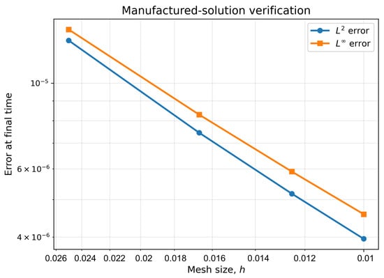
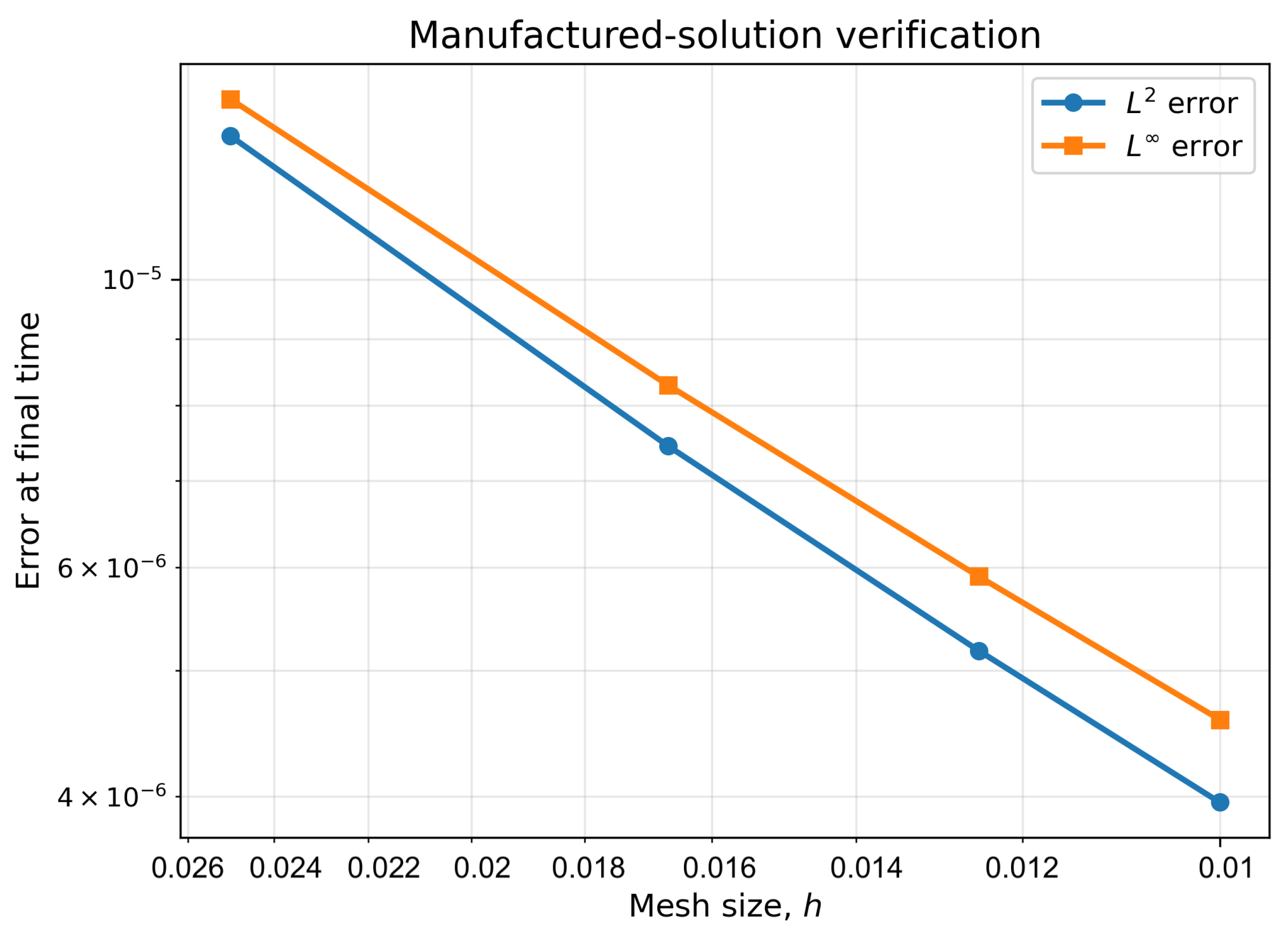
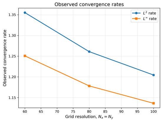
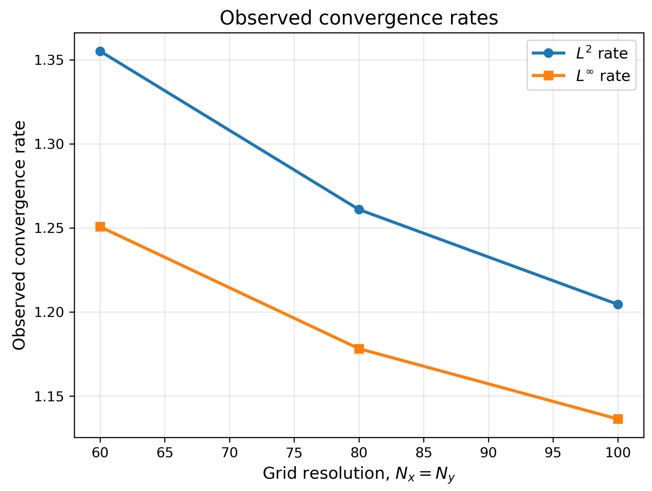
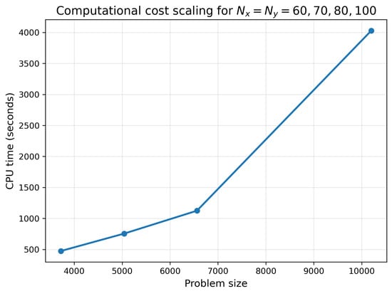
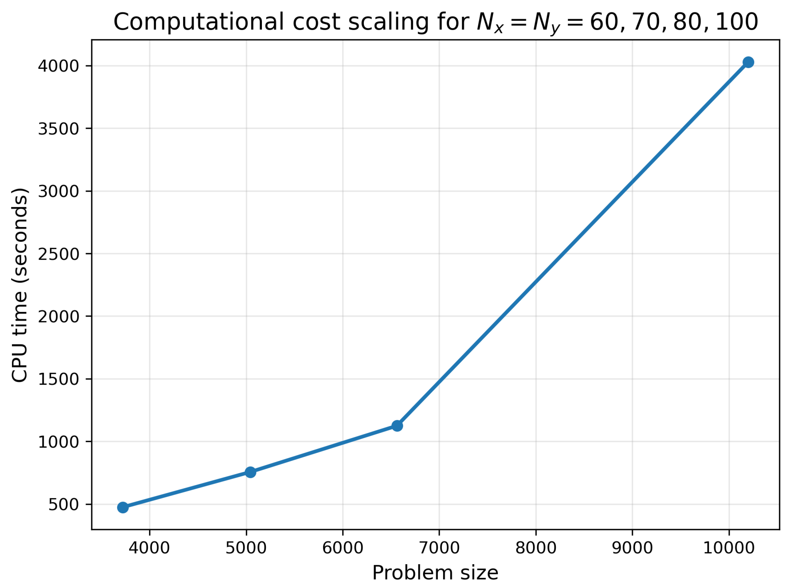
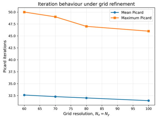
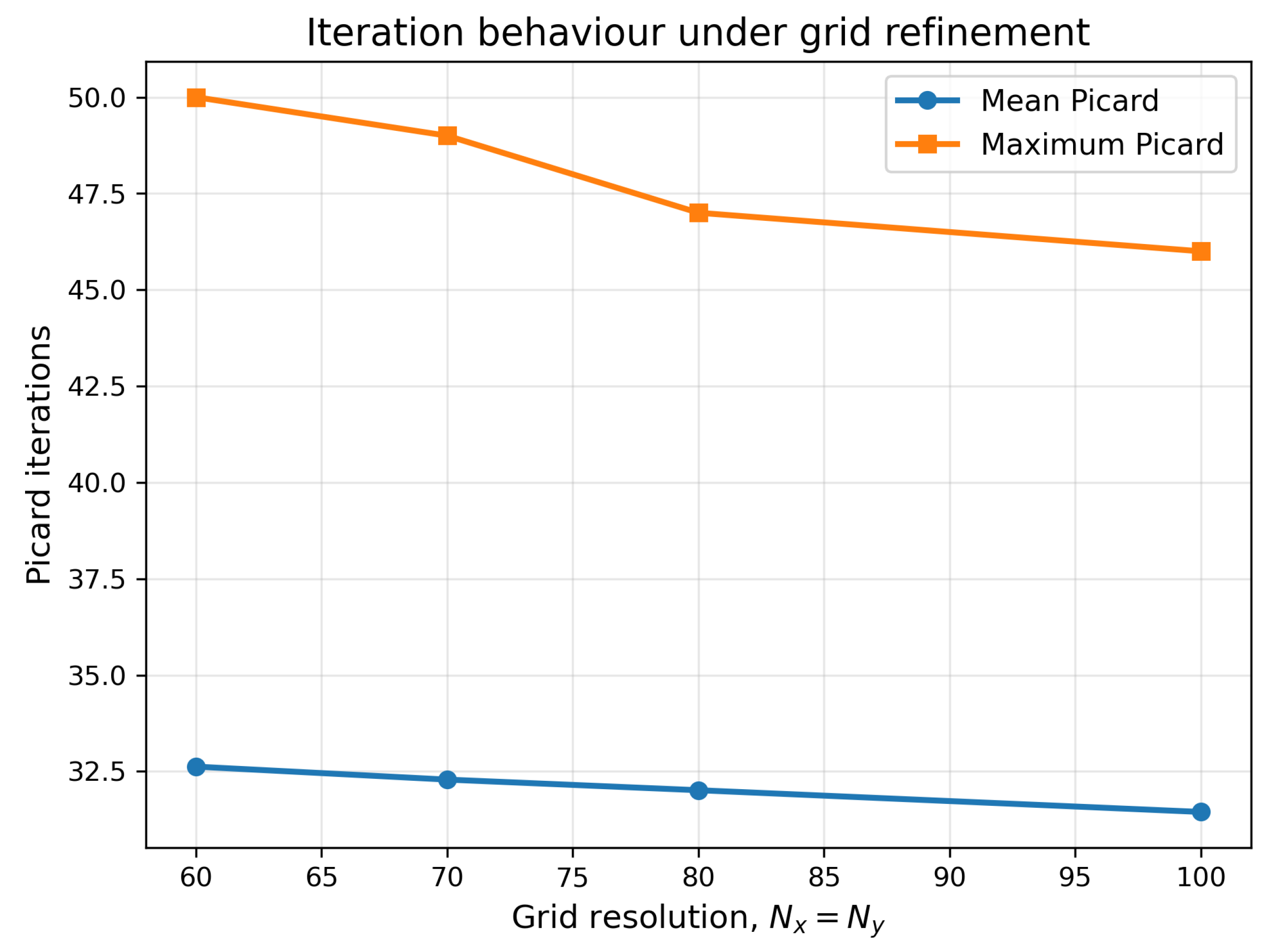
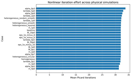
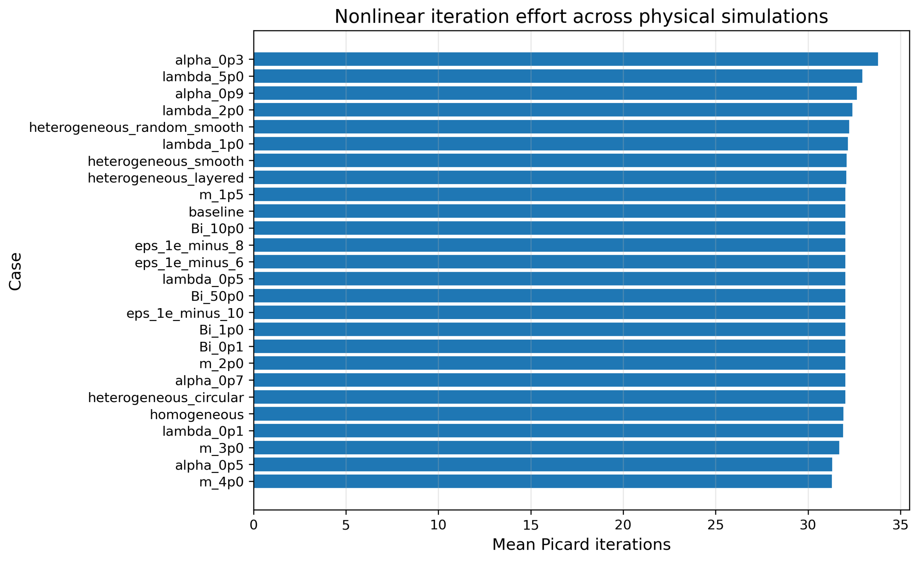
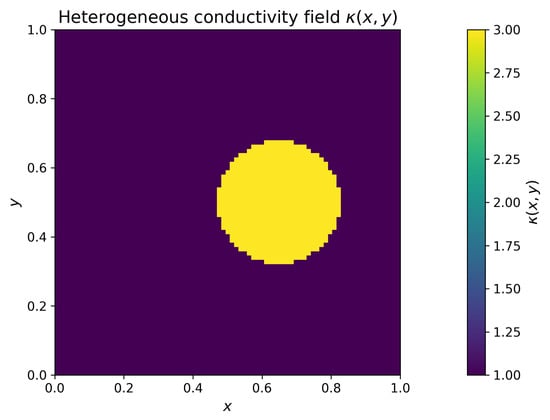
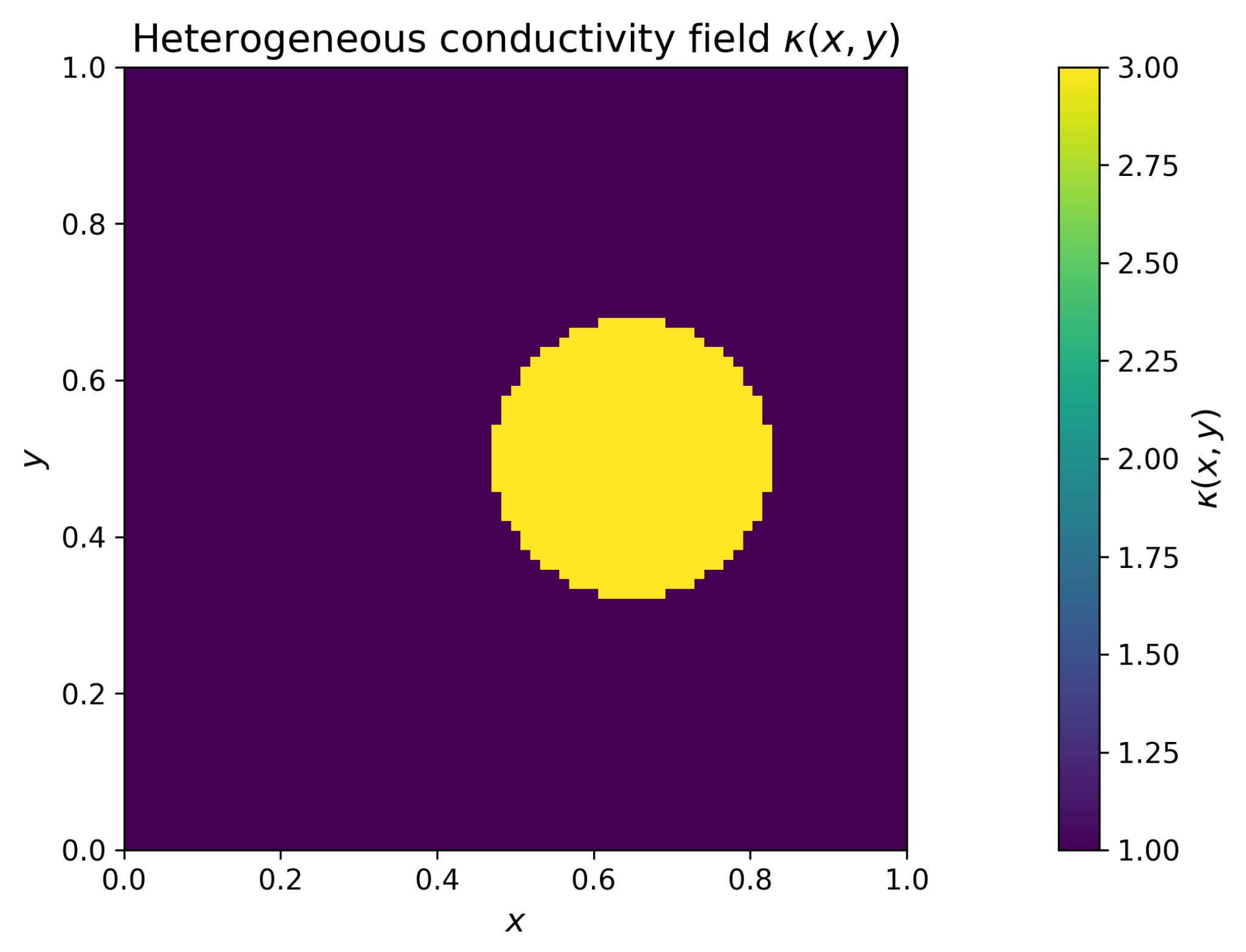
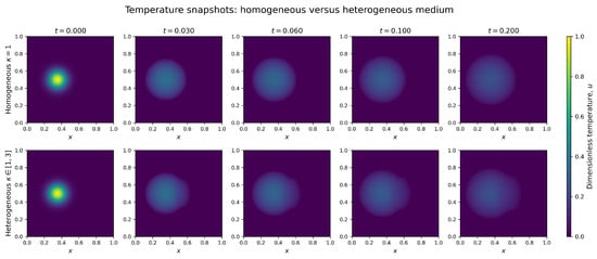
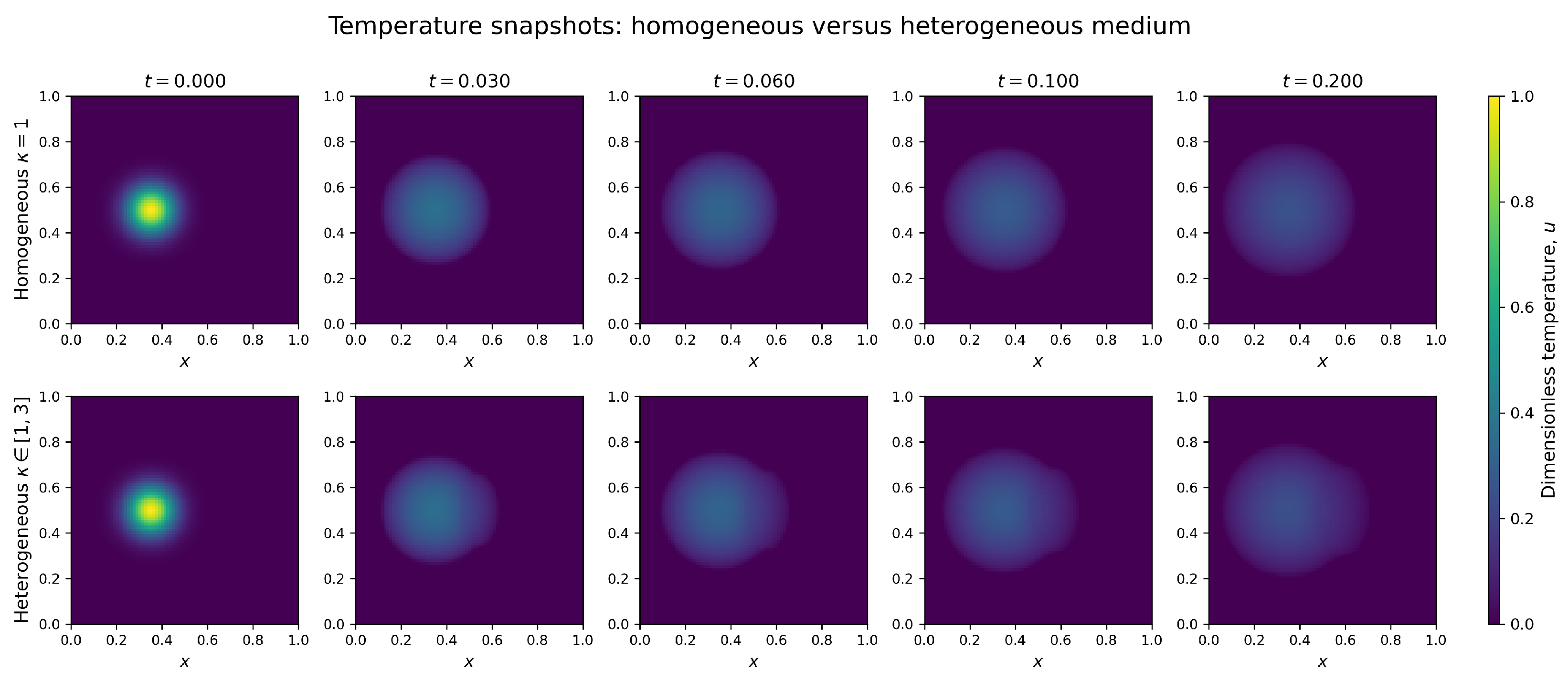
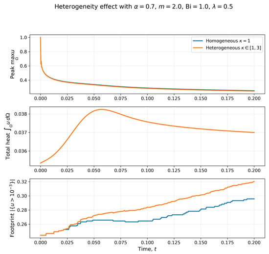
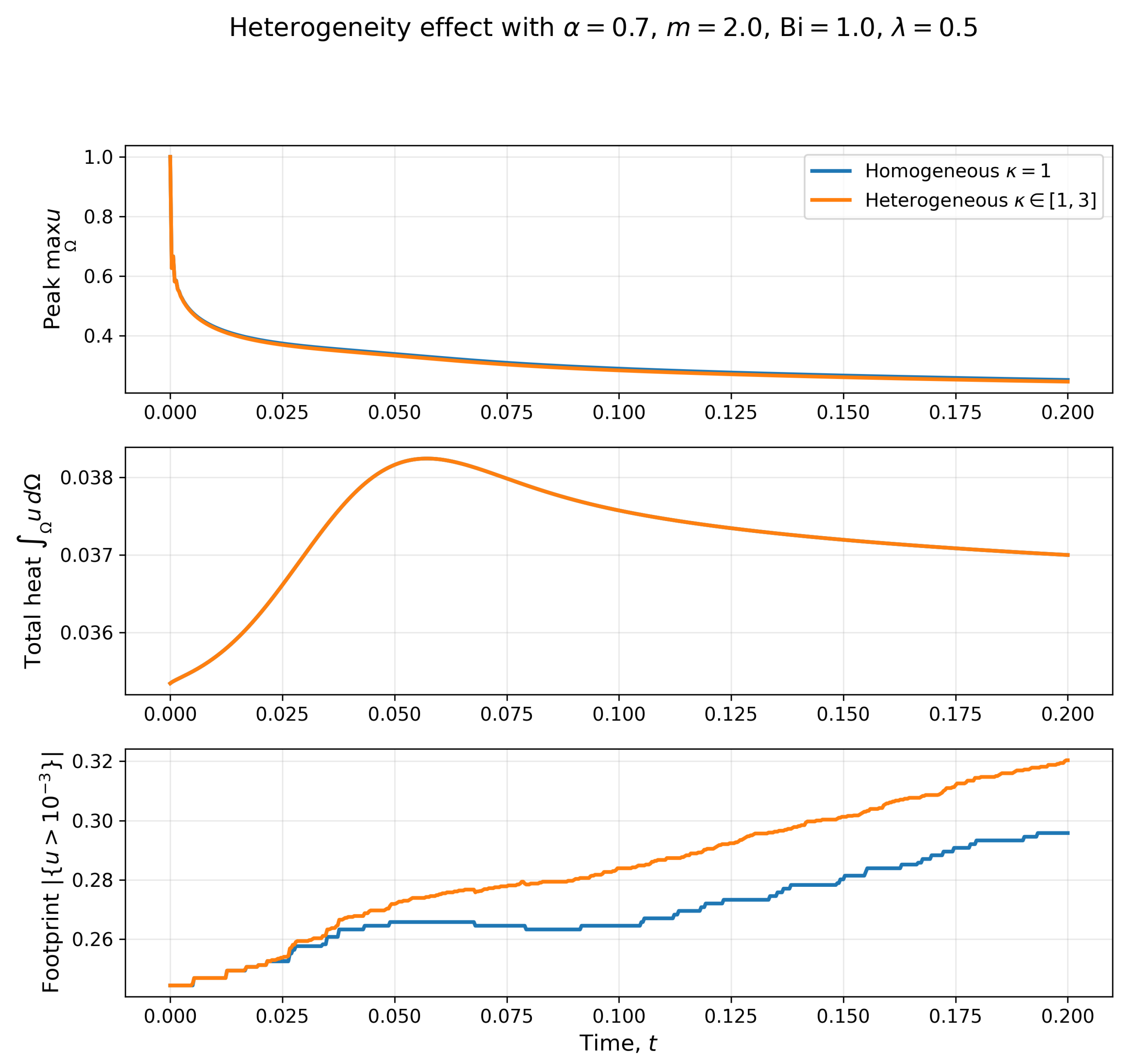
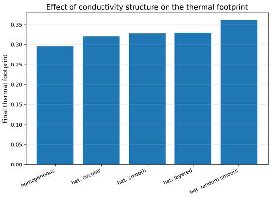
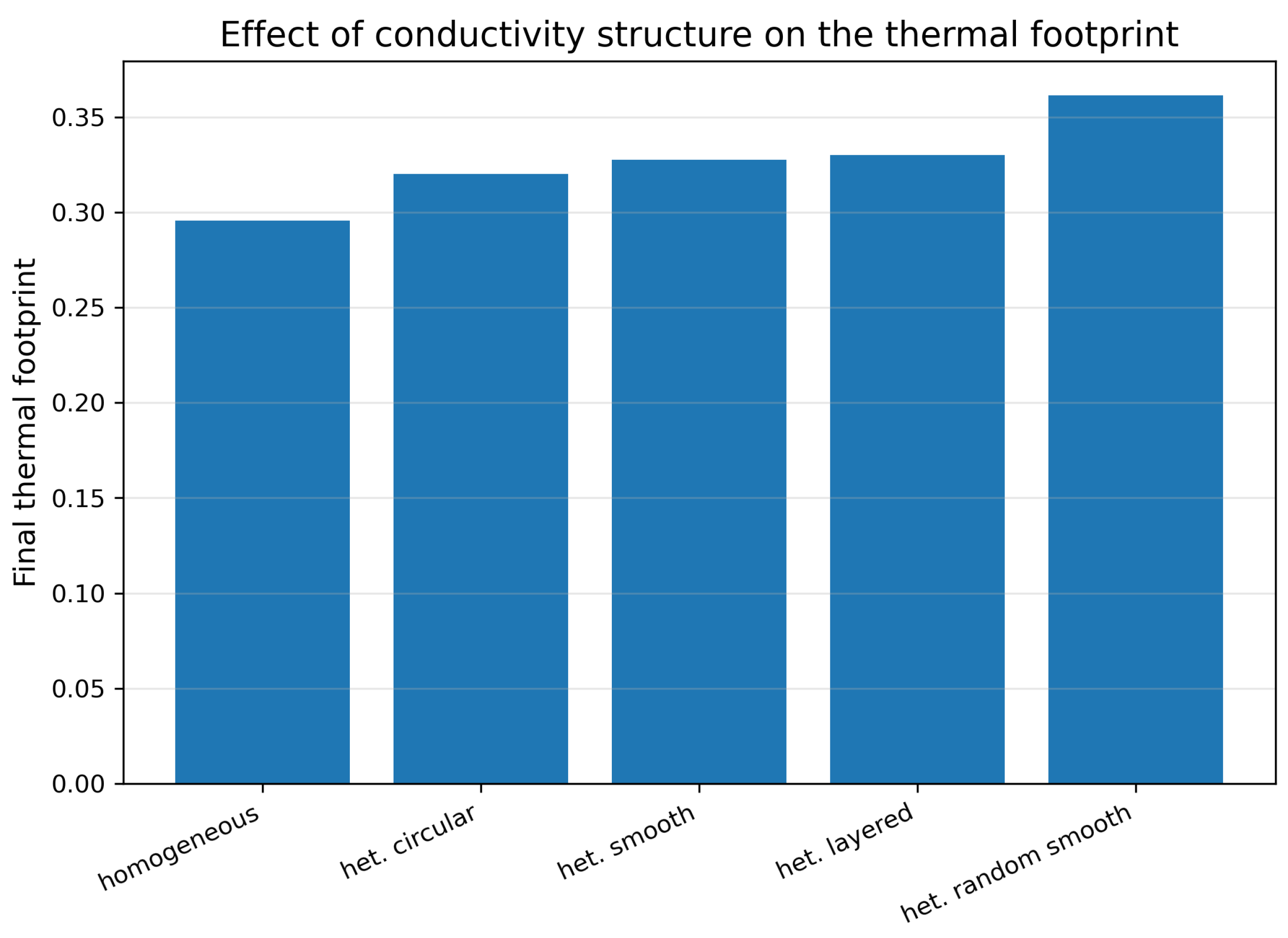
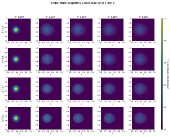
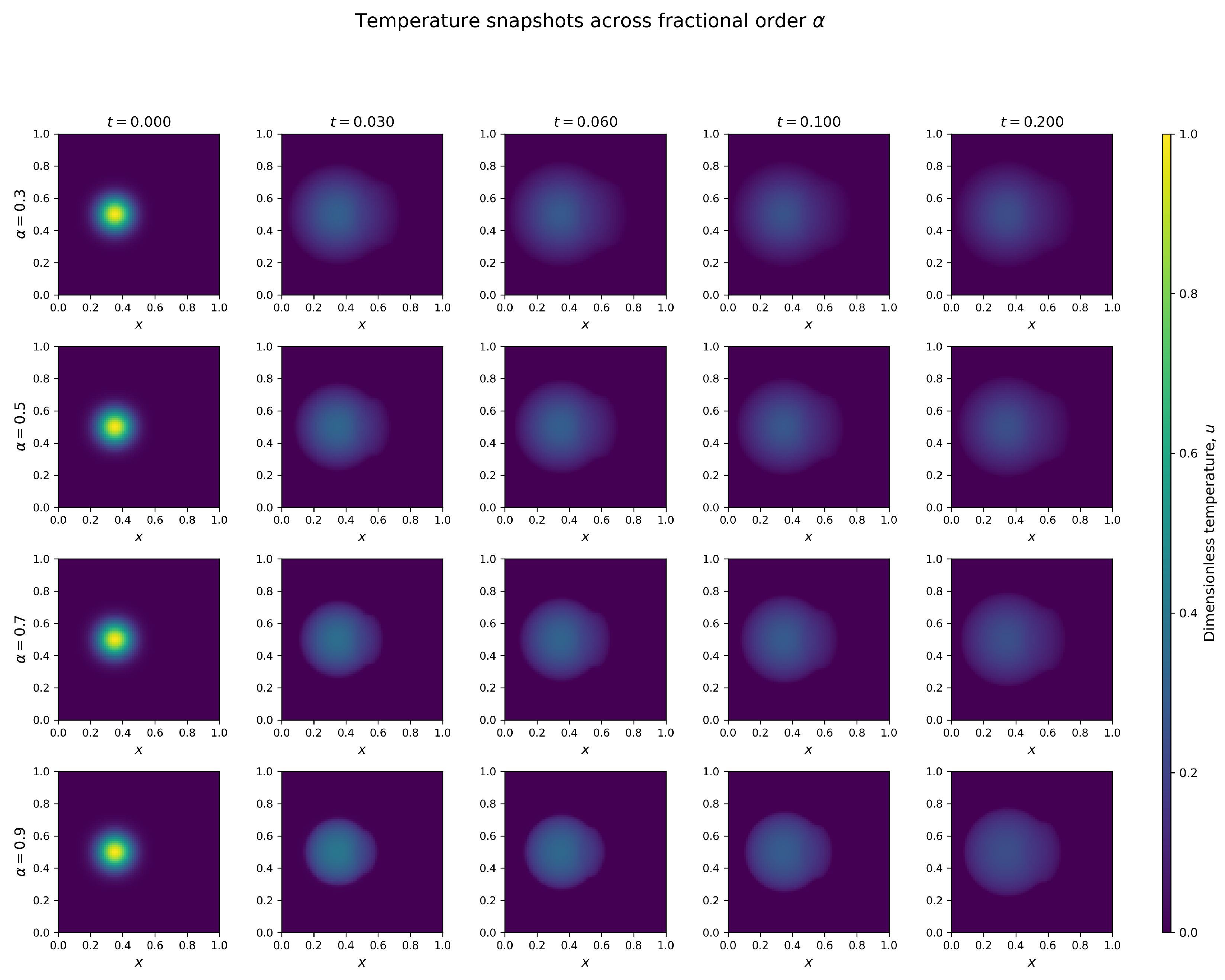
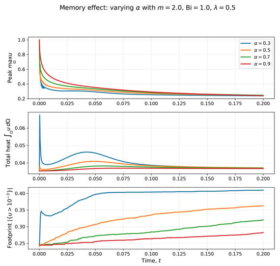
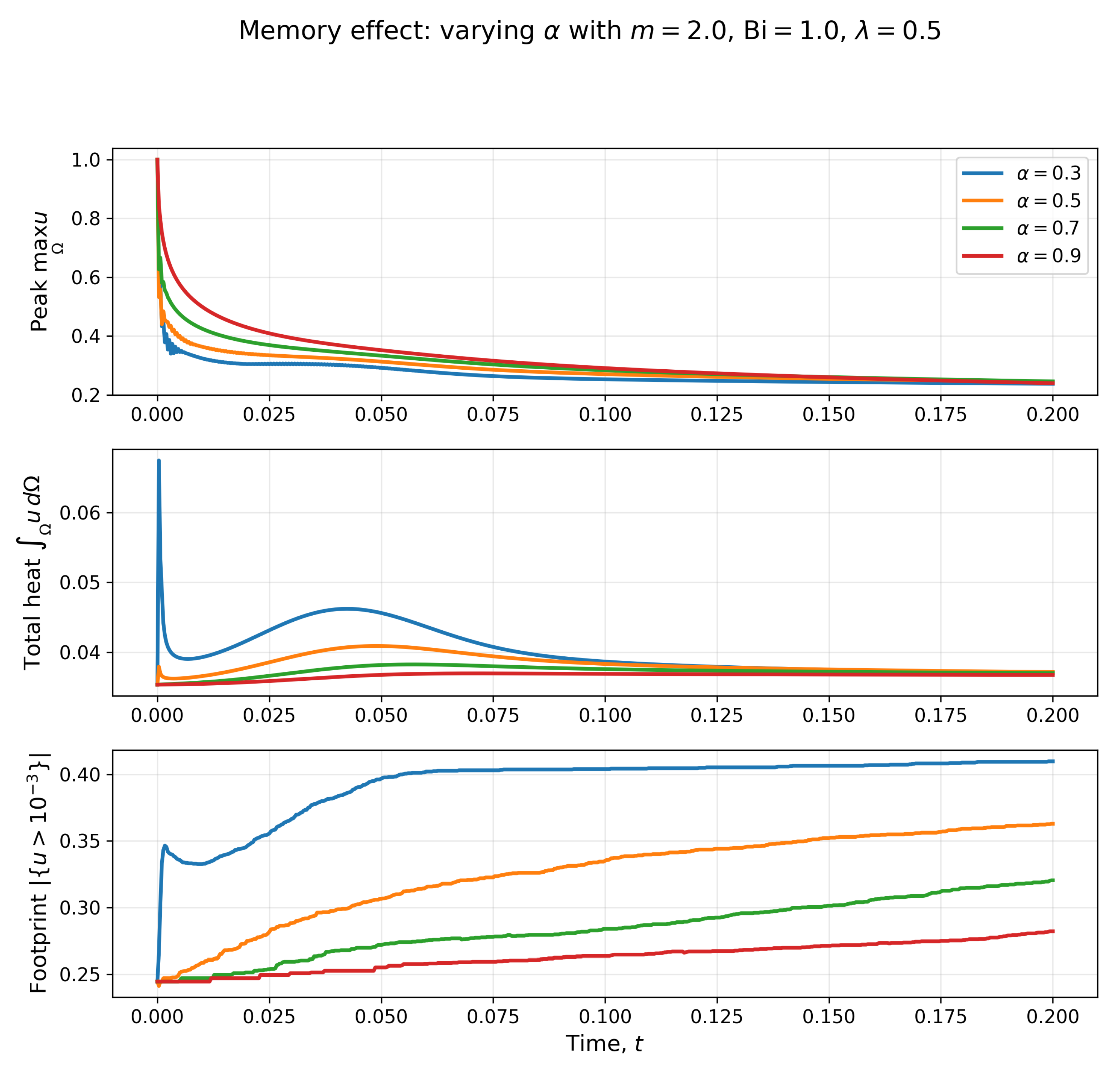
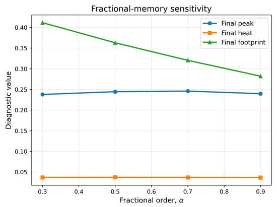
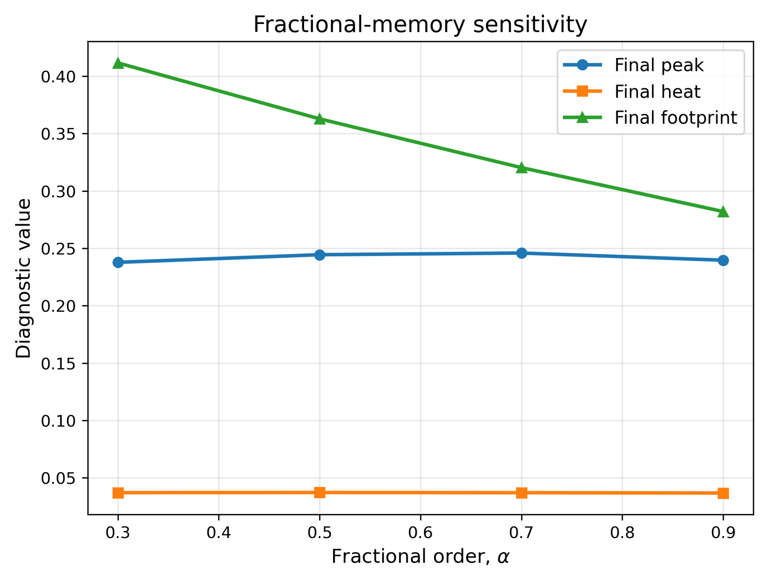
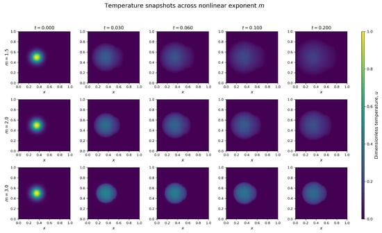
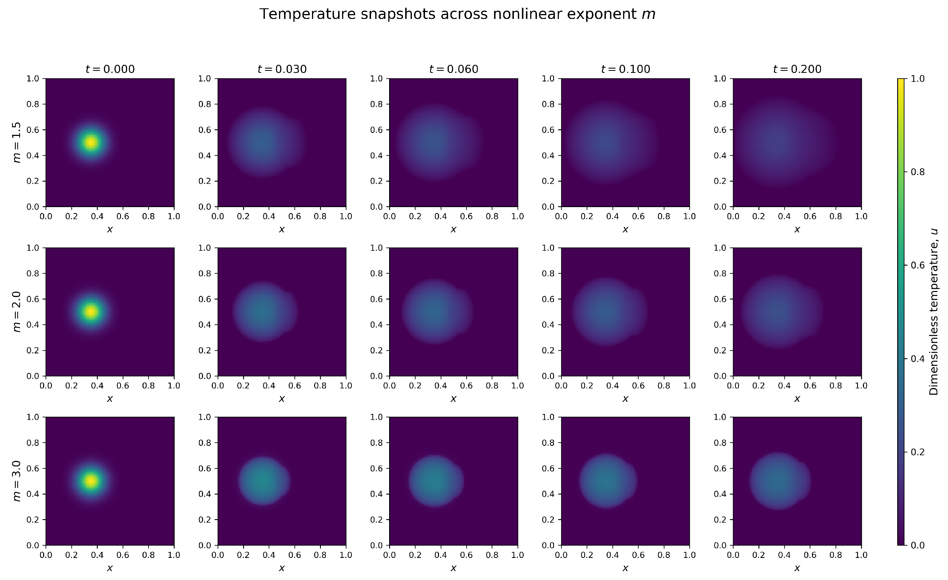
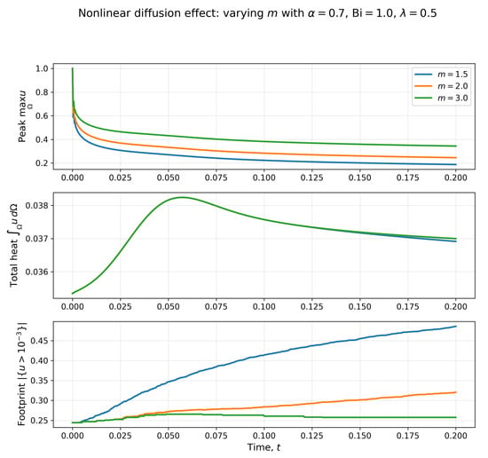
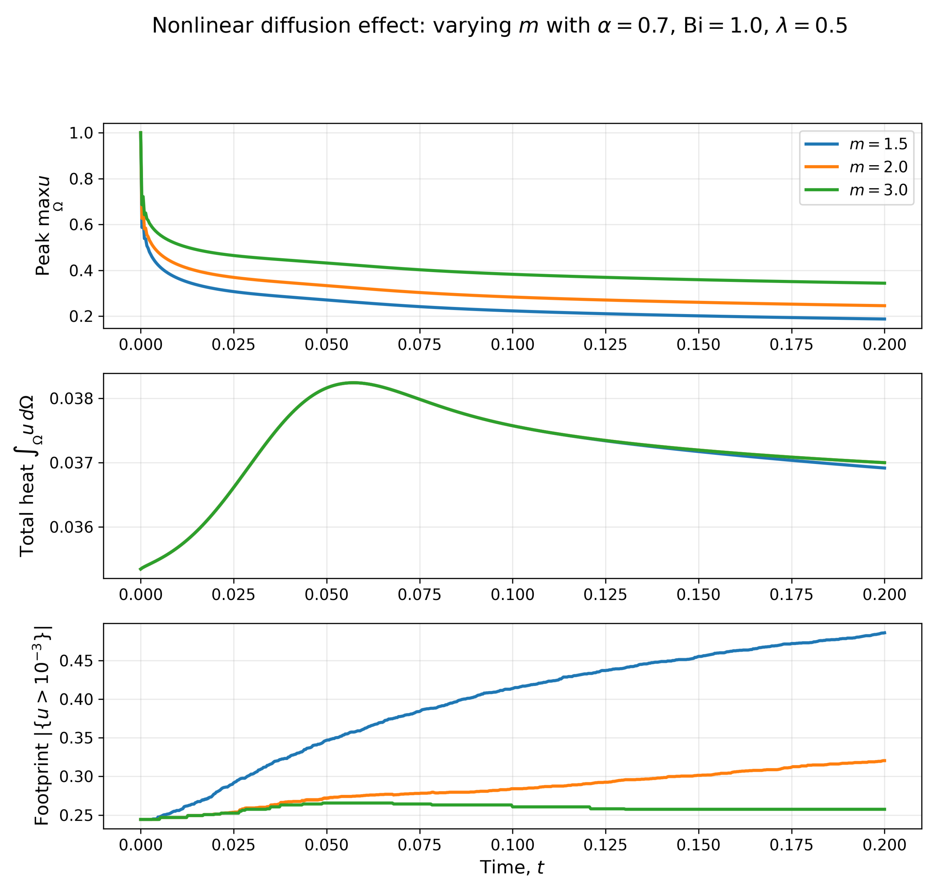
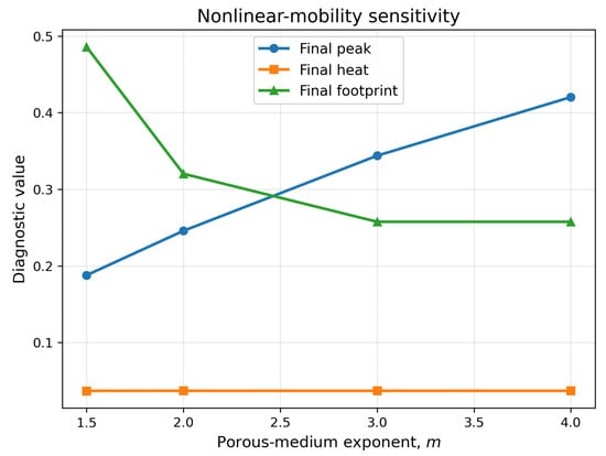
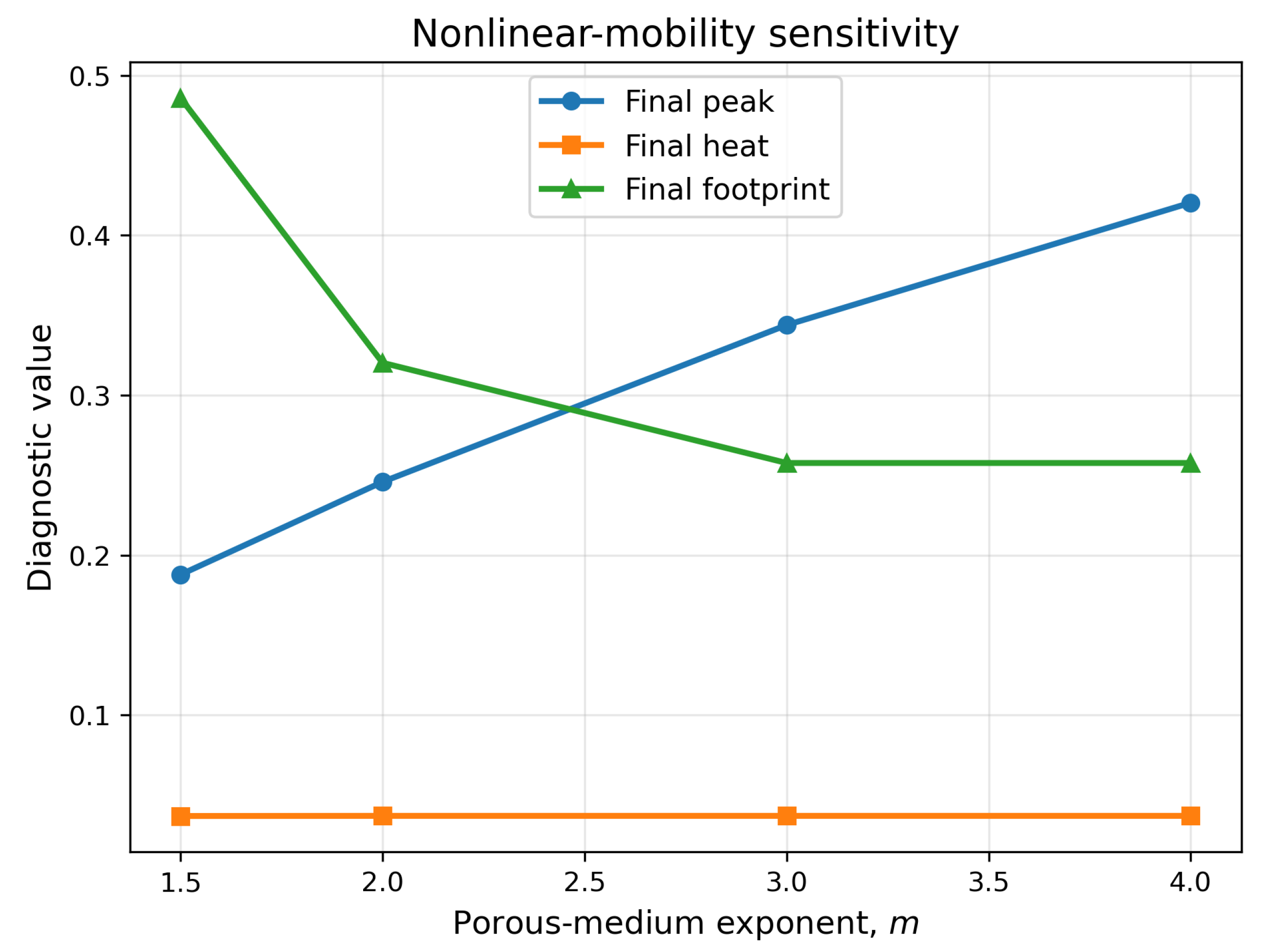
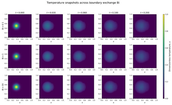
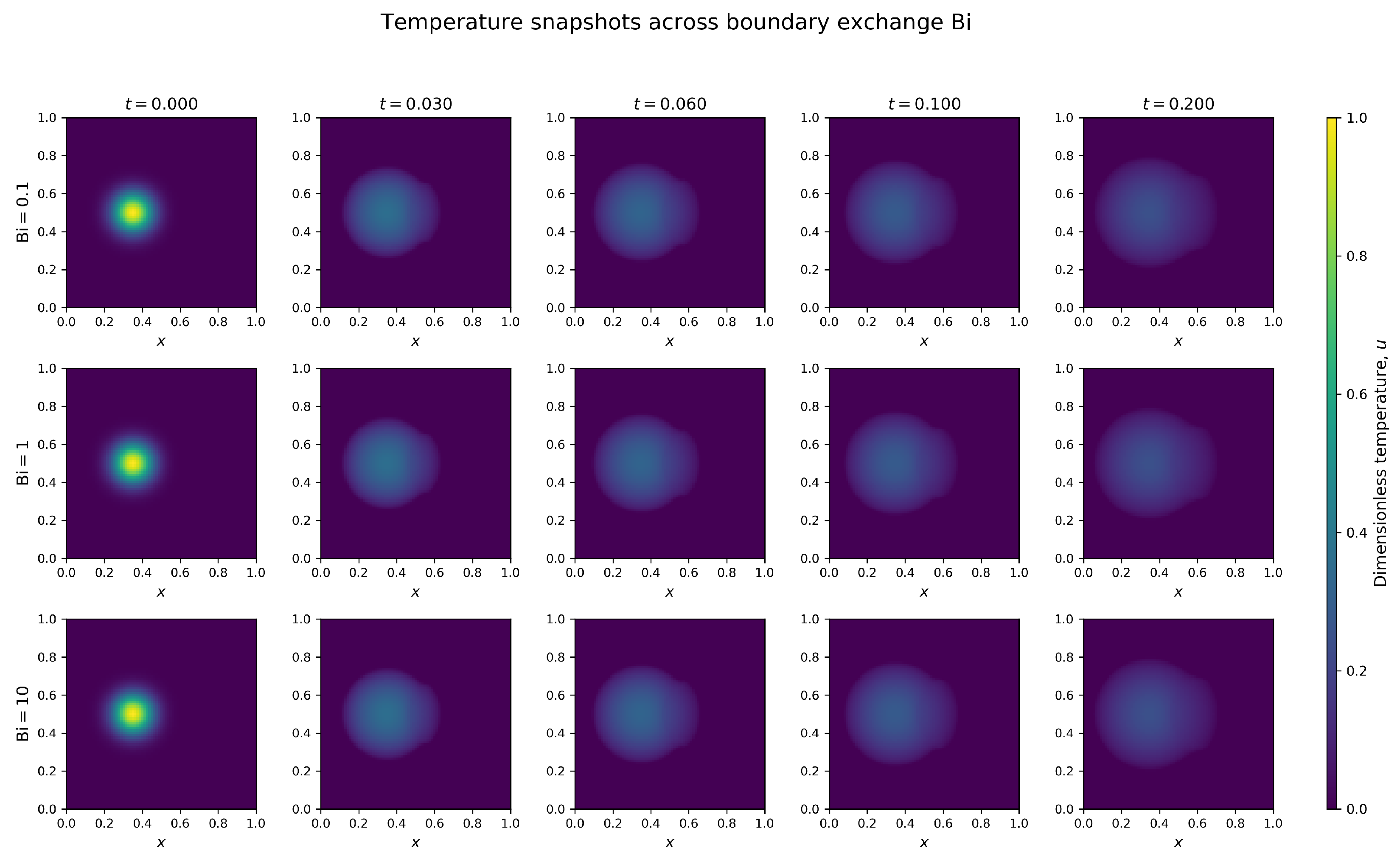
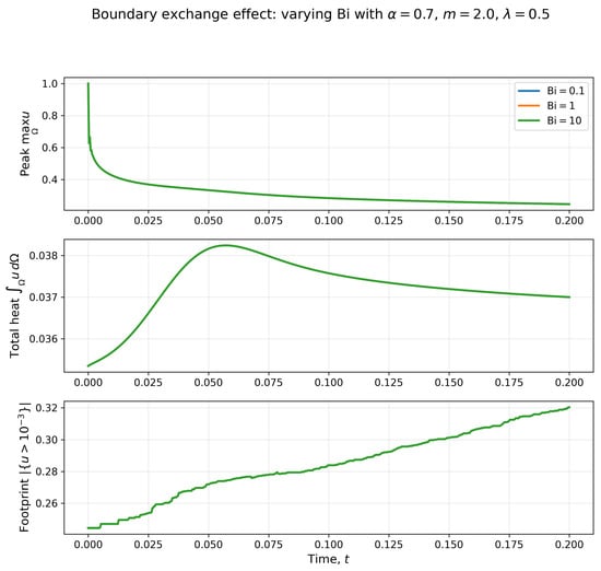
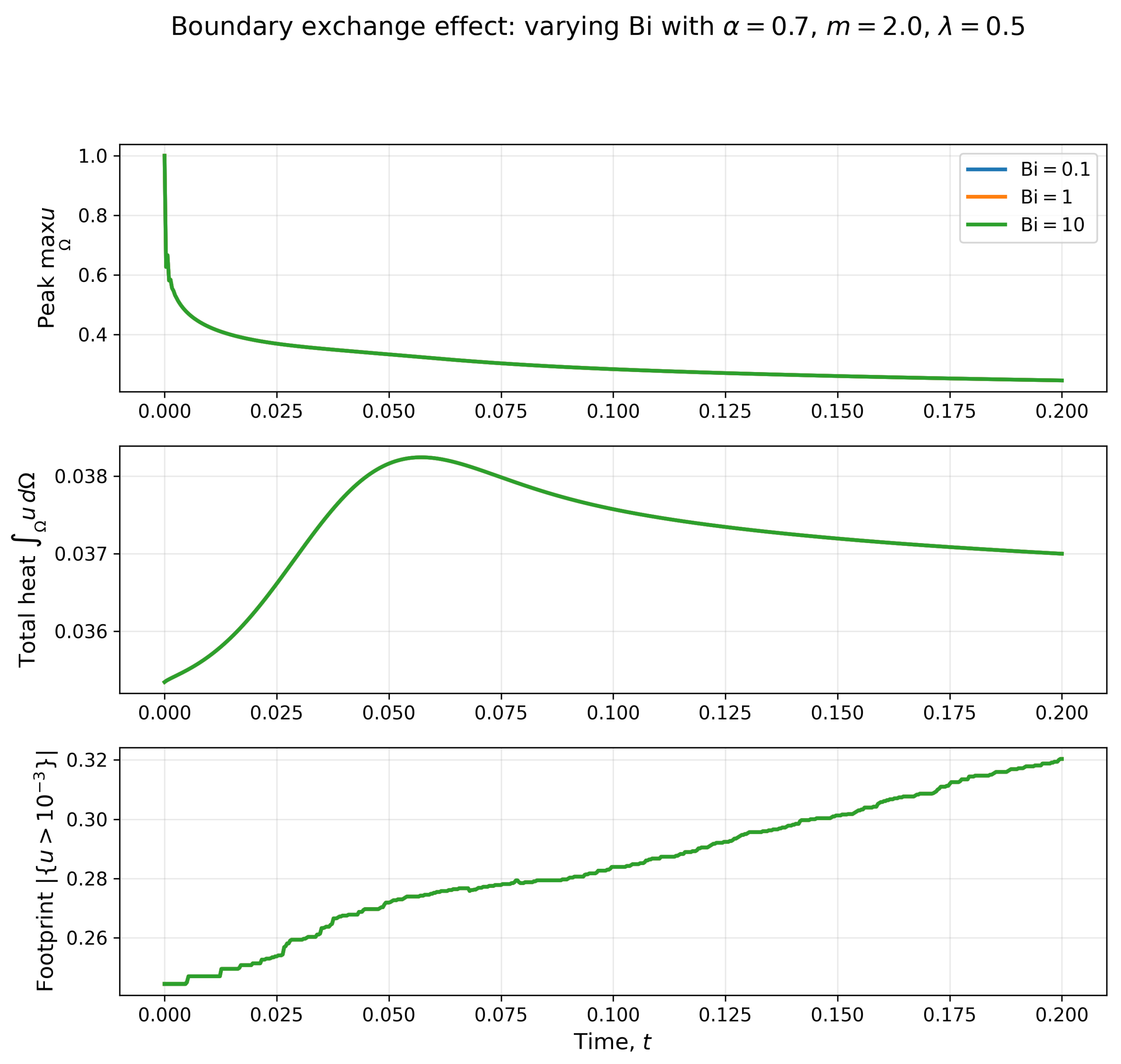
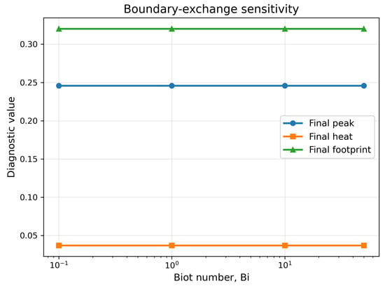
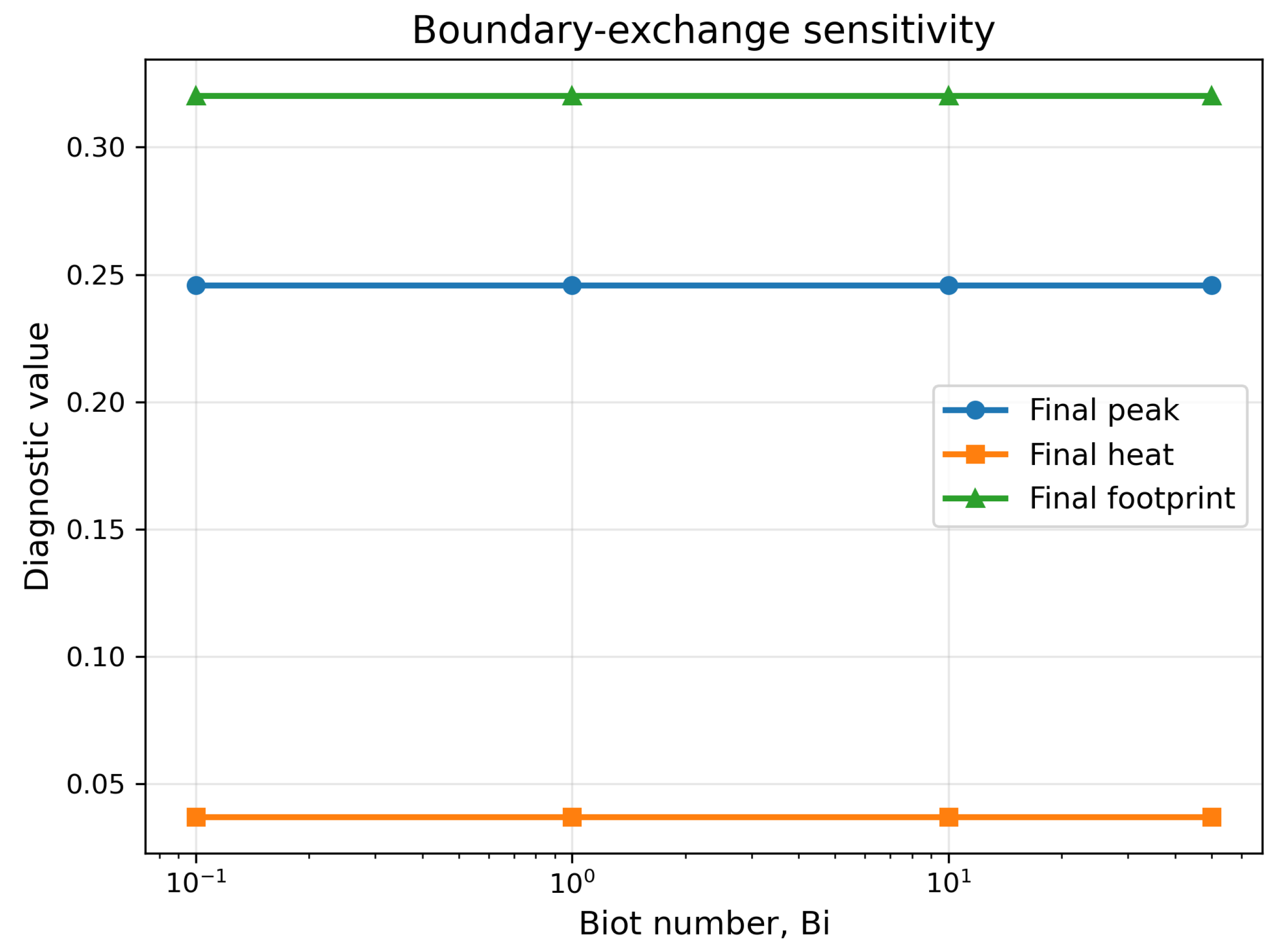
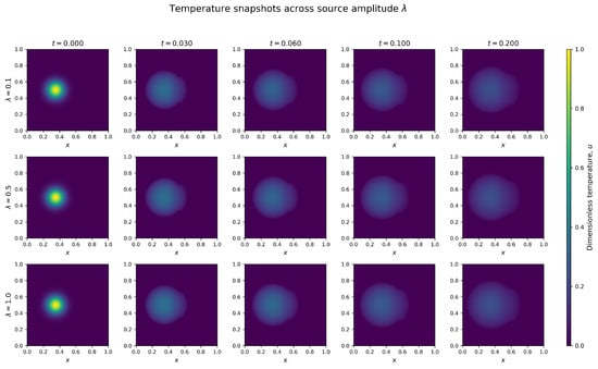
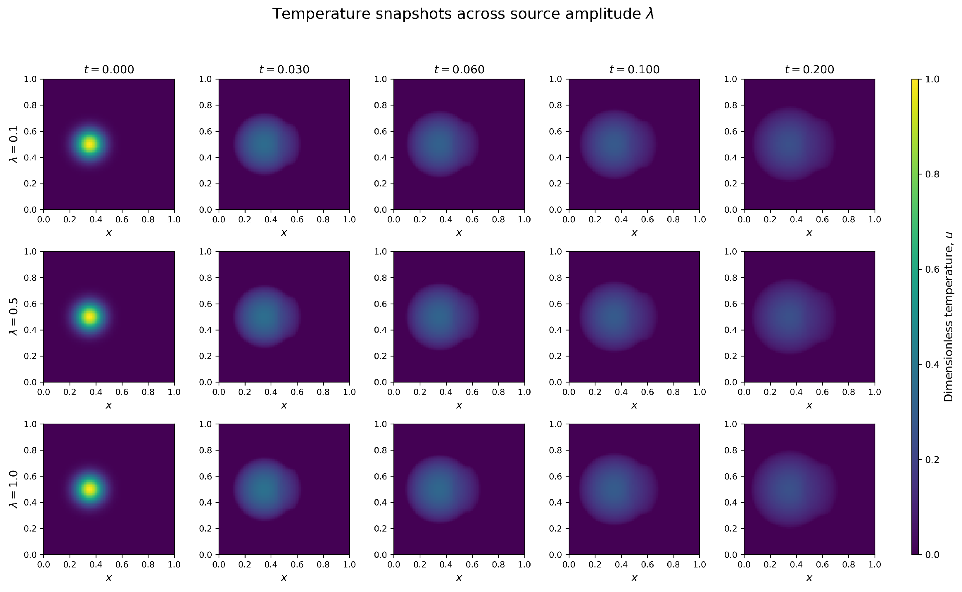
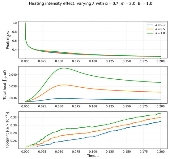
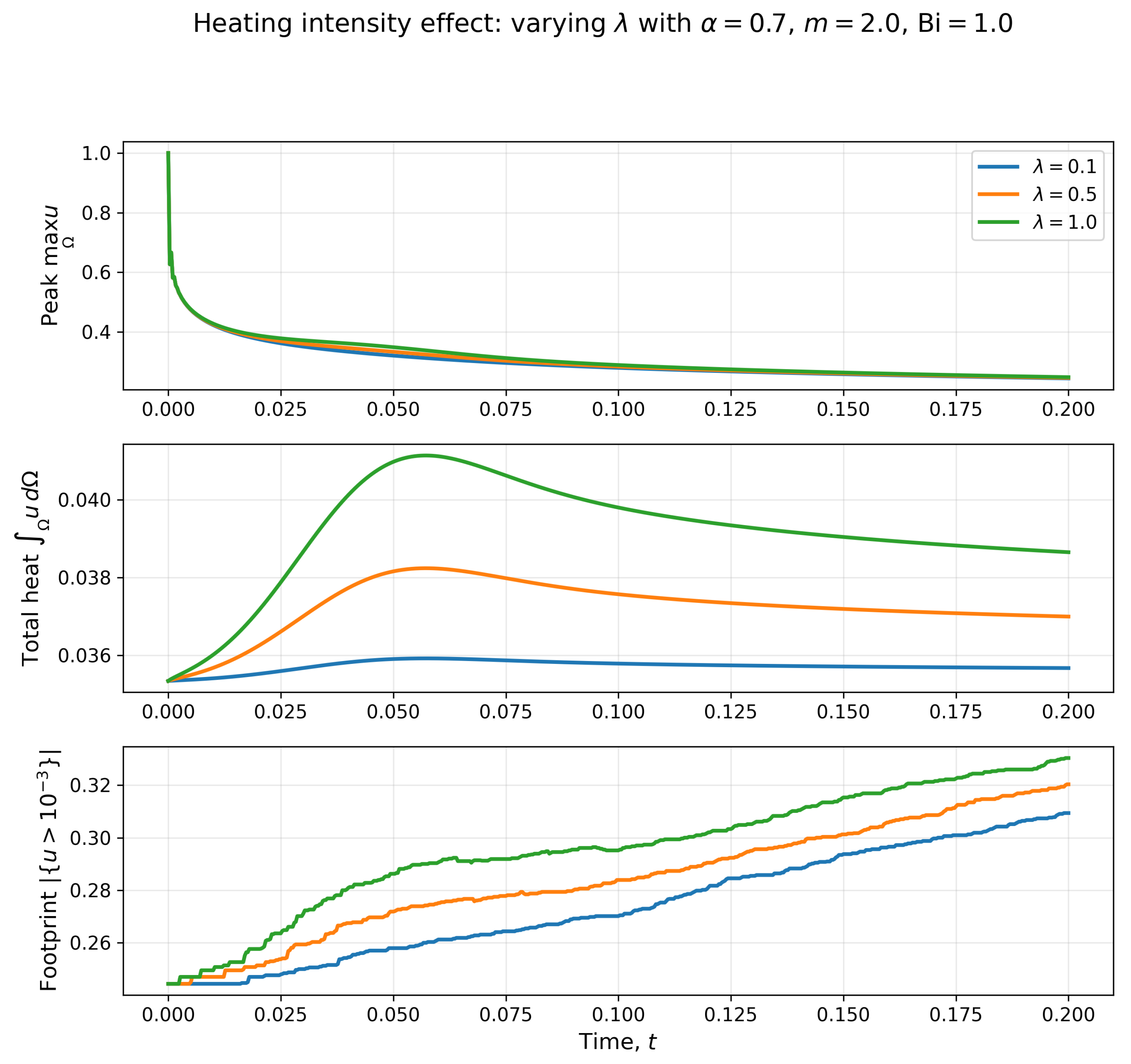
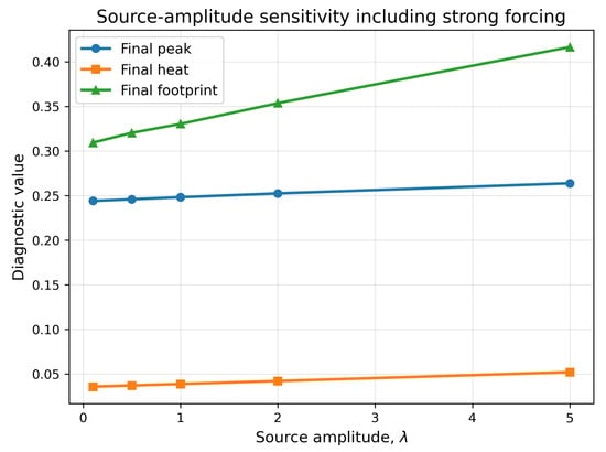
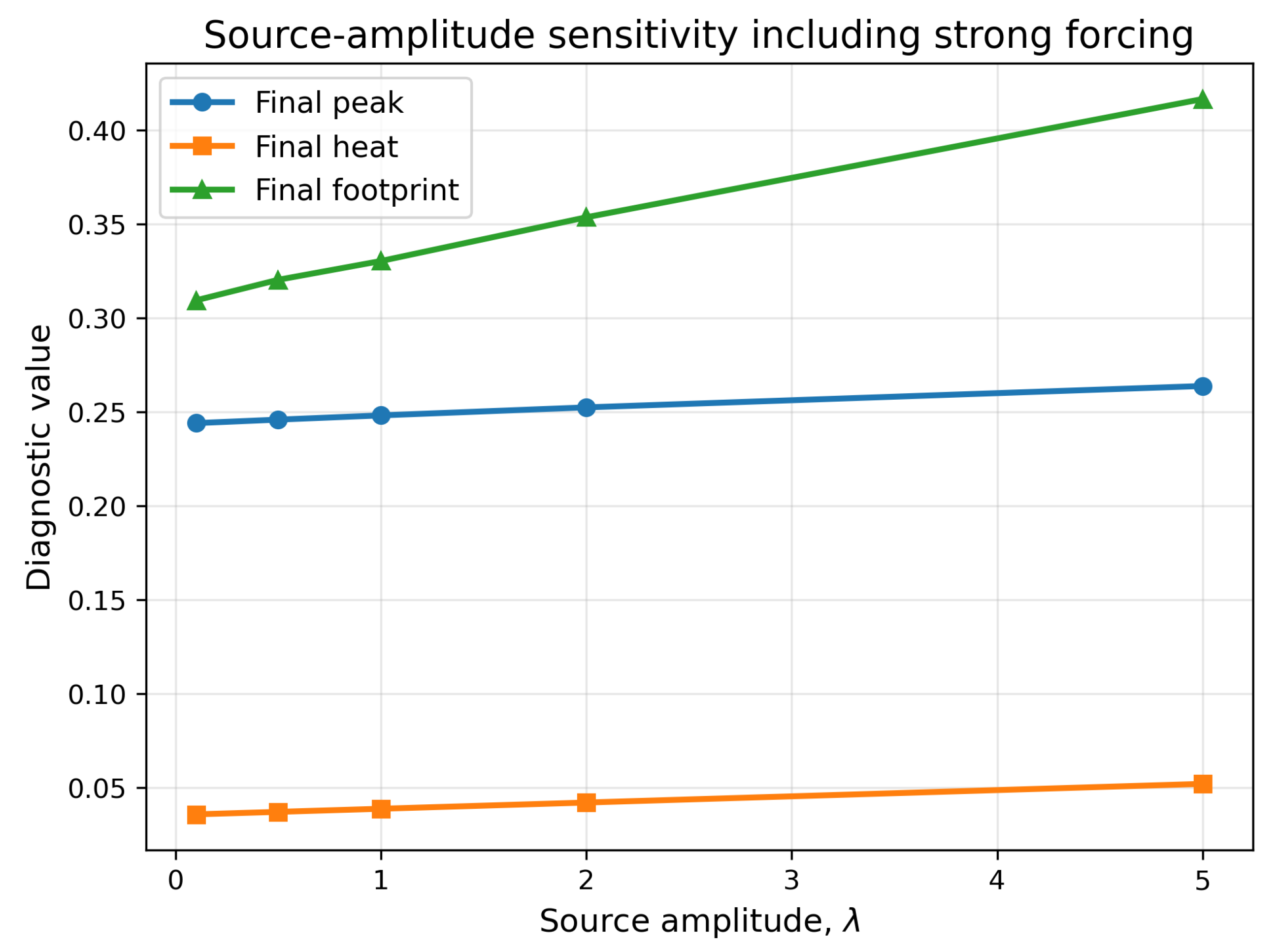
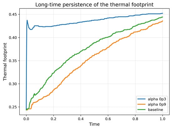
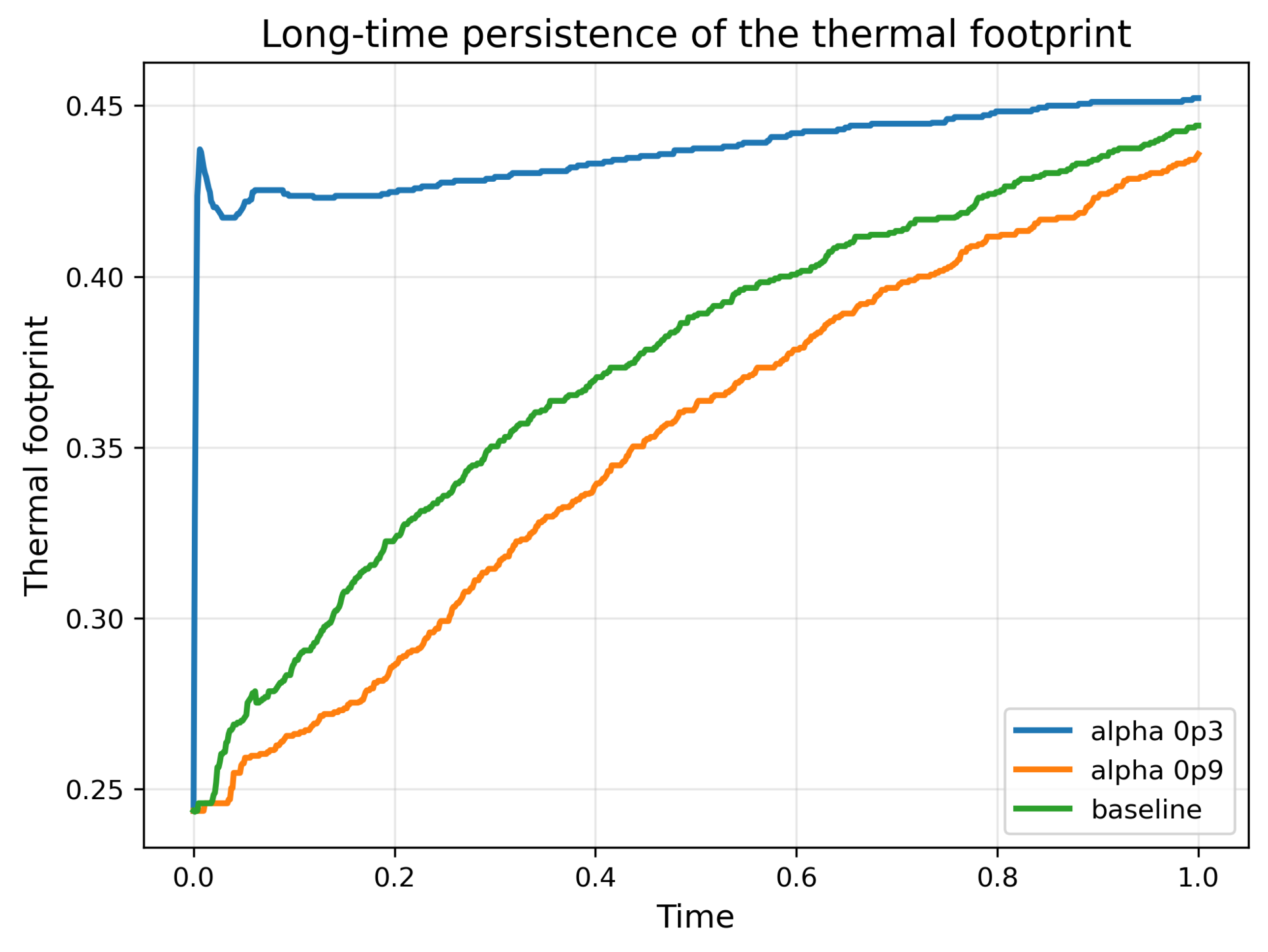

Disclaimer/Publisher’s Note: The statements, opinions and data contained in all publications are solely those of the individual author(s) and contributor(s) and not of MDPI and/or the editor(s). MDPI and/or the editor(s) disclaim responsibility for any injury to people or property resulting from any ideas, methods, instructions or products referred to in the content. |
© 2026 by the authors. Licensee MDPI, Basel, Switzerland. This article is an open access article distributed under the terms and conditions of the Creative Commons Attribution (CC BY) license.