Coexistence States for a Non-Cooperative Model Arising in Reactor Dynamics with Heat Exchange

Abstract

The existence of coexistence states of a non-cooperative nuclear reactor model is investigated in this paper. Differently from the existing literature, we allow the nonlinearities to not necessarily be linearizable at zero and infinity, and the boundary condition in the model implies that the nuclear reactor has heat exchange with the external environment, which much more closely reflects the situation in reality. Several novel existence theorems distinct from existing results in the literature are established by means of bifurcation theory. Our main findings will not only be helpful to enrich the related theories of nuclear reactor models but also have certain guiding significance for the safe operation of reactors.

1. Introduction

This paper concerns the existence of coexistence states of the following non-cooperative mathematical model:

$$\left\{\begin{array}{c}-\Delta u=\lambda f(x,u)-b\left(x\right)uv,x\in \mathrm{\Omega },\hfill \\ -\Delta v=c\left(x\right)u-d\left(x\right)uv-e\left(x\right)v,x\in \mathrm{\Omega },\hfill \\ u=0,{\displaystyle \frac{\partial v}{\partial \mathbf{n}}}+\alpha \left(x\right)v=0,x\in \partial \mathrm{\Omega },\hfill \end{array}\right.$$

(1)

which arises in nuclear reactor dynamics. Here, a pair $(\lambda ,(u,v\left)\right)$ is called a coexistence state of (1) if $u\gg 0,v\gg 0$, that is, $(u,v)\in C^2\left(\overline{\mathrm{\Omega }}\right)\times C^2\left(\overline{\mathrm{\Omega }}\right)$ with $u>0$ in $\mathrm{\Omega }$ and $u=0$ on $\partial \mathrm{\Omega }$ [1]; meanwhile, $v>0$ on $\overline{\mathrm{\Omega }}$. We assume that $\mathrm{\Omega }\subset {\mathbb{R}}^N(N\ge 1)$ is a bounded connected domain with the boundary $\partial \mathrm{\Omega }$ of class $C^2$ and indicates the closed container, $\mathbf{n}$ is the unit outward normal vector on $\partial \mathrm{\Omega }$, the coefficient functions $b,c,d,e\in C\left(\overline{\mathrm{\Omega }}\right)$ are positive and $\lambda >0$ is a parameter, $f:\overline{\mathrm{\Omega }}\times [0,\infty )\to [0,\infty )$ is continuous; and $\alpha \in C^{1+\theta }(\partial \mathrm{\Omega })(0<\theta <1)$ is the heat exchange coefficient taking positive values. It is worth pointing out that the boundary condition in (1) implies that there are no fast neutrons on the boundary of the closed container $\mathrm{\Omega }$, and the nuclear reactor exchanges heat energy with the outside environment, which much more closely reflects the situation in reality [2].

As is well known, model (1) is closely related to the parabolic system

$$\left\{\begin{array}{c}{u}_t-\Delta u=au-buv,x\in \mathrm{\Omega },t>0,\hfill \\ v_t-\Delta v=cu-duv-ev,x\in \mathrm{\Omega },t>0,\hfill \end{array}\right.$$

(2)

which refines the model proposed by Kastenberg et al. [3] by adding the diffusion and the nonlinear feedback to the temperature [4], where $\Delta v$ is the diffusion of the temperature, $a,b,c,d$ and e are positive constants, b denotes the negative feedback of the temperature, and $duv+ev$ denotes the nonlinear feedback to the temperature. In real-world applications, the unknown functions u and v stand for the density of fast neutrons and the temperature in the reactor, respectively.

Over the past few decades, system (2), subject to different boundary conditions such as Dirichlet and Neumann types, has been of great interest to many authors; see [1,4,5,6,7,8,9,10] and references therein. Several researchers have also paid attention to one-dimensional analogs of the model; see for instance [5,11,12,13,14,15] for more details.

It is worth remarking that in most of the papers mentioned above, the models were studied under homogeneous Dirichlet boundary condition, and a was frequently viewed as a bifurcation parameter. For example, Arioli [5] studied the existence of nontrivial periodic solutions and the global attractor of (2), and López-Gómez [5] mainly discussed the corresponding steady state problem. Some researchers [1,6,7,8,9,10] completed and sharpened the corresponding ones established in [4,5], and especially in [10], the authors obtained a new necessary and sufficient condition to guarantee the existence of coexistence states of model (2) subject to the Neumann boundary condition.

For some earlier research works on this topic, one can be referred to [2,16,17,18,19] and the references therein. Additionally, for results related to model (1) under the resonant case, as well as recently developed nonconforming finite element methods for it, we further refer the reader to [20,21,22].

As far as we know, however, the study on the existence of coexistence states for spatially heterogeneous models is progressing much more slowly, and the existing results related to model (1), where the boundary condition means the nuclear reactor has heat exchange with the external environment, remain relatively scarce. Since the heat exchange boundary condition reflects the situation much more closely to reality, the research results on model (1) shall be practically more useful for the efficient and safe operation of the reactor. In view of this, we are interested in this work to determine the values of $\lambda >0$, for which there are coexistence states for a more general non-cooperative model (1).

To this end, we assume the following throughout the paper:

• (A1) $f:\overline{\mathrm{\Omega }}\times [0,\infty )\to [0,\infty )$ is continuous, $f(x,s)>0$ for any $x\in \overline{\mathrm{\Omega }}$ and $s>0$.
• (A2) There are positive constants $f^0,f_0,f^{\infty }$ and $f_{\infty }$, such that

  $$f_{0}s-{\zeta }_1(x,s)\le f(x,s)\le f^{0}s+{\zeta }_2(x,s)$$

  for some ${\zeta }_i\in C(\overline{\mathrm{\Omega }}\times [0,\infty ))$ with ${\zeta }_i(x,s)=\circ \left(s\right)$ as $s\to 0$ uniformly for $x\in \overline{\mathrm{\Omega }}$, and

  $$f_{\infty }s-{\xi }_1(x,s)\le f(x,s)\le f^{\infty }s+{\xi }_2(x,s)$$

  for some ${\xi }_i\in C(\overline{\mathrm{\Omega }}\times [0,\infty ))$ with ${\xi }_i(x,s)=\circ \left(s\right)$ as $s\to \infty$ uniformly for $x\in \overline{\mathrm{\Omega }}$, $i=1,2$.

Obviously, (A2) implies the nonlinear term f is not necessarily linearizable at 0 and $+\infty$. Moreover, we replace $au$ with the nonlinear term $\lambda f(x,u)$, which shall be helpful to restore the actual physical process of the reactor and improve the accuracy of transient predictions. For convenience, we denote by $\lambda (-\Delta +\chi )$ the principal eigenvalue of

$$\left\{\begin{array}{c}-\Delta u+\chi \left(x\right)u=\lambda u,x\in \mathrm{\Omega },\hfill \\ u=0,x\in \partial \mathrm{\Omega }\hfill \end{array}\right.$$

for some measurable function $\chi$ on $\mathrm{\Omega }$, and let ${\lambda }_1=\lambda (-\Delta )$, which corresponds to the principal eigenfunction ${\phi }_1\gg 0$ satisfying $\parallel {\phi }_1{\parallel }_{\infty }=\underset{x\in \overline{\mathrm{\Omega }}}{\max }\left|{\phi }_1\left(x\right)\right|=1$. Setting

$$I_0=\left[{\displaystyle \frac{{\lambda }_1}{f^0}},{\displaystyle \frac{{\lambda }_1}{f_0}}\right],$$

$$I_{\infty }=\left[{\displaystyle \frac{\lambda (-\Delta +bc/d)}{f^{\infty }}},{\displaystyle \frac{\lambda (-\Delta +bc/d)}{f_{\infty }}}\right].$$

Our main results can be stated as follows.

Theorem 1.

Assume (A1) and (A2). Then (1) admits a coexistence state if either

$${\displaystyle \frac{{\lambda }_1}{f_0}}<\lambda <{\displaystyle \frac{\lambda (-\Delta +bc/d)}{f^{\infty }}},$$

or

$${\displaystyle \frac{\lambda (-\Delta +bc/d)}{f_{\infty }}}<\lambda <{\displaystyle \frac{{\lambda }_1}{f^0}}.$$

Remark 1.

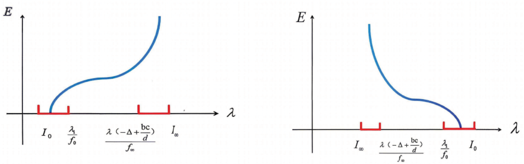
The following bifurcation diagrams in Figure 1 demonstrate the bifurcation phenomena of nuclear reactor model (1).

The rest of the paper is arranged as below. In Section 2, we give some preliminaries that are required to prove Theorem 1. We shall prove our main result Theorem 1 in Section 3, and some related results will also be presented to demonstrate the feasibility of our main findings in Section 4.

2. Preliminaries

The proof of Theorem 1 follows from some preliminary lemmas to be established in this section.

Lemma 1.

Assume (A1) and (A2). If $(\lambda ,(u,v\left)\right)$ is a nonnegative nontrivial solution of (1), then $u\gg 0,v\equiv 0$ and $v\left(x\right)\le {\parallel c/d\parallel }_{\infty }$ for all $x\in \overline{\mathrm{\Omega }}$. Moreover, $\lambda \in \Lambda$ for some bounded interval $\Lambda \subset [0,\infty )$.

Proof. 

We first show that if $(\lambda ,(u,v\left)\right)$ is a nonnegative nontrivial solution of (1), then $u\ge 0,\not\equiv 0$ and $v\ge 0,\not\equiv 0$. Indeed, if $u=0$, then from the v equation of (1) it follows that

$$\left\{\begin{array}{c}-\Delta v+e\left(x\right)v=0,x\in \mathrm{\Omega },\hfill \\ v=0,x\in \partial \mathrm{\Omega },\hfill \end{array}\right.$$

and so $v=0$. On the other hand, if $v=0$, then the v equation of (1) gives $c\left(x\right)u=0$ again, and thus $u=0$. Consequently, $u\ge 0,\not\equiv 0$ and $v\ge 0,\not\equiv 0.$

Next we define, for $x\in \overline{\mathrm{\Omega }}$,

$$\omega \left(x\right)=\left\{\begin{array}{c}{\displaystyle \frac{f(x,u(x\left)\right)}{u\left(x\right)}},u\left(x\right)>0,\hfill \\ f_0,u\left(x\right)=0,\hfill \end{array}\right.$$

so it is not difficult to see that $\omega$ is positive on $\overline{\mathrm{\Omega }}$, since $u\ge 0,\not\equiv 0$, and by (A2) and the u equation of (1) we can obtain

$$\left\{\begin{array}{c}(-\Delta +b(x\left)v\right)u\ge \lambda \omega \left(x\right)u,x\in \mathrm{\Omega },\hfill \\ u=0,x\in \partial \mathrm{\Omega },\hfill \end{array}\right.$$

and the strong maximum principle yields $u\gg 0$. We claim that ${\parallel v\parallel }_{\infty }\le {\parallel c/d\parallel }_{\infty }.$ Indeed, if v achieves its maximum at some $x_0\in \mathrm{\Omega }$, then $v\left(x_0\right)={\parallel v\parallel }_{\infty }>0$, and it follows easily $-\Delta v\left(x_0\right)\ge 0$, and the v equation of (1) gives

$$\left(c\left(x_0\right)-d\left(x_0\right)v\left(x_0\right)\right)u\left(x_0\right)\ge e\left(x_0\right)v\left(x_0\right)>0,$$

which yields ${\parallel v\parallel }_{\infty }<{\parallel c/d\parallel }_{\infty }$. On the other hand, if there is $x_0\in \partial \mathrm{\Omega }$ so that $v\left(x_0\right)={\parallel v\parallel }_{\infty }>0$, then we can obtain $v\left(x_0\right)\le {\parallel c/d\parallel }_{\infty }$. Suppose on the contrary that $v\left(x_0\right)>{\parallel c/d\parallel }_{\infty }$; then there is an open ball $B\subset \mathrm{\Omega }$ with a sufficiently small radius, such that B is tangent to the boundary $\partial \mathrm{\Omega }$ at $x_0$ and ${v\left(x\right)>\parallel c/d\parallel }_{\infty }$ for any $x\in B$, and subsequently,

$$-\Delta v+e\left(x\right)v=\left(c\left(x\right)-d\left(x\right)v\right)u<0,x\in B,$$

this, together with the Hopf’s lemma [23], yields ${\displaystyle \frac{\partial v}{\partial \mathbf{n}}}\left(x_0\right)>0$, which contradicts the boundary condition satisfied by v. Therefore,

$${\parallel v\parallel }_{\infty }\le {\parallel c/d\parallel }_{\infty }.$$

It follows from (A1) and (A2) that there are positive constants $f_{\ast },f^{\ast }$ such that

$$0<f_{\ast }\le {\displaystyle \frac{f(x,s)}{s}}\le f^{\ast },x\in \overline{\mathrm{\Omega }},s\in [0,\infty ),$$

hence ${\mu }_{\ast }<\lambda <{\mu }^{\ast }$, where ${\mu }^{\ast }={\displaystyle \frac{\lambda (-\Delta +b\left(x\right)\parallel c/d{\parallel }_{\infty })}{f_{\ast }}}$ and ${\mu }_{\ast }={\displaystyle \frac{{\lambda }_1}{f^{\ast }}}$ stand for, respectively, the principal eigenvalue of

$$\left\{\begin{array}{c}{-\Delta u+b\left(x\right)\parallel c/d\parallel }_{\infty }u=\mu f_{\ast }u,x\in \mathrm{\Omega },\hfill \\ u=0,x\in \partial \mathrm{\Omega }\hfill \end{array}\right.$$

and

$$\left\{\begin{array}{c}-\Delta u=\mu f^{\ast }u,x\in \mathrm{\Omega },\hfill \\ u=0,x\in \partial \mathrm{\Omega }.\hfill \end{array}\right.$$

Consequently, $\lambda \in \Lambda =({\mu }_{\ast },{\mu }^{\ast })\subset [0,\infty )$.

Finally, let us show $v\gg 0$. We first prove $v\left(x\right)>0$ for $x\in \mathrm{\Omega }$. Otherwise, if there is $x_1\in \mathrm{\Omega }$ such that $v\left(x_1\right)=0$, then $\nabla v\left(x_1\right)=0$ and $\Delta v\left(x_1\right)\ge 0$. However, by the v equation of (1) we get $-\Delta v\left(x_1\right)=c\left(x_1\right)u\left(x_1\right)>0$, which leads to a contradiction. Since $u\gg 0$, we can deduce from the v equation of (1) that

$$\left\{\begin{array}{c}-\Delta v+\left(d\left(x\right)u+e\left(x\right)\right)v=c\left(x\right)u>0,x\in \mathrm{\Omega },\hfill \\ {\displaystyle \frac{\partial v}{\partial \mathbf{n}}}+\alpha \left(x\right)v=0,x\in \partial \mathrm{\Omega },\hfill \end{array}\right.$$

and the strong maximum principle gives $v\gg 0$. □

In the following, set

$$r_0={\displaystyle \frac{f^0+f_0}{2}},d_0={\displaystyle \frac{f^0-f_0}{2}}$$

and

$$g(x,s)=f(x,s)-r_{0}s$$

for $x\in \overline{\mathrm{\Omega }}$ and $s\in [0,\infty )$. Then from (A2) it follows

$$-d_{0}s-{\zeta }_1(x,s)\le g(x,s)\le d_{0}s+{\zeta }_2(x,s)$$

(3)

as $s\to 0$, and (1) can be equivalently written as

$$\left\{\begin{array}{c}-\Delta u=\lambda r_{0}u+\lambda g(x,u)-b\left(x\right)uv,x\in \mathrm{\Omega },\hfill \\ -\Delta v=c\left(x\right)u-d\left(x\right)uv-e\left(x\right)v,x\in \mathrm{\Omega },\hfill \\ u=0,{\displaystyle \frac{\partial v}{\partial \mathbf{n}}}+\alpha \left(x\right)v=0,x\in \partial \mathrm{\Omega }.\hfill \end{array}\right.$$

(4)

To prove Theorem 1, let us consider the auxiliary problem

$$\left\{\begin{array}{c}-\Delta u=\lambda r_{0}u+{\lambda g(x,|u|}^{\epsilon }u)-b\left(x\right)uv,x\in \mathrm{\Omega },\hfill \\ -\Delta v=c\left(x\right)u-d\left(x\right)uv-e\left(x\right)v,x\in \mathrm{\Omega },\hfill \\ u=0,{\displaystyle \frac{\partial v}{\partial \mathbf{n}}}+\alpha \left(x\right)v=0,x\in \partial \mathrm{\Omega },\hfill \end{array}\right.$$

(5)

where $\epsilon \in [0,1]$ is a parameter.

Lemma 2.

Assume that $\left\{{\epsilon }_n\right\}\subset [0,1]$ with ${\epsilon }_n\to 0$ as $n\to \infty$. If there is a sequence $\{{\lambda }_n,(u_n,v_n)\}\subset (0,\infty )\times E$ such that $({\lambda }_n,(u_n,v_n))$ is a coexistence state of (5) corresponding to $\epsilon ={\epsilon }_n$, and

$$({\lambda }_n,(u_n,v_n))\to (\lambda ,(0,0))$$

in $(0,\infty )\times E$ as $n\to \infty$, then $\lambda \in I_0$. Here E is the usual Banach space $C_0^1\left(\overline{\mathrm{\Omega }}\right)\times C^1\left(\overline{\mathrm{\Omega }}\right)$.

Proof. 

For $n\ge 1$, let

$${\check{u}}_n={\displaystyle \frac{u_n}{\parallel u_n{\parallel }_{\infty }}},{\check{v}}_n={\displaystyle \frac{v_n}{\parallel u_n{\parallel }_{\infty }}},$$

then ${\check{u}}_n$ and ${\check{v}}_n$ satisfy

$$\left\{\begin{array}{c}-\Delta {\check{u}}_n={\lambda }_n{r}_0{\check{u}}_n+{\lambda }_n{\displaystyle \frac{g(x,|u_n{|}^{{\epsilon }_n}{u}_n)}{\parallel u_n{\parallel }_{\infty }}}-b\left(x\right)v_n{\check{u}}_n,x\in \mathrm{\Omega },\hfill \\ -\Delta {\check{v}}_n=c\left(x\right){\check{u}}_n-d\left(x\right)v_n{\check{u}}_n-e\left(x\right){\check{v}}_n,x\in \mathrm{\Omega },\hfill \\ {\check{u}}_n=0,{\displaystyle \frac{\partial {\check{v}}_n}{\partial \mathbf{n}}}+\alpha \left(x\right){\check{v}}_n=0,x\in \partial \mathrm{\Omega }.\hfill \end{array}\right.$$

(6)

Since $({\lambda }_n,(u_n,v_n))$ is a coexistence state of (5) corresponding to $\epsilon ={\epsilon }_n$, similar to the proof of Lemma 1, we can get for each $n\ge 1$ that

$$\parallel v_n{\parallel }_{\infty }\le {\parallel c/d\parallel }_{\infty }.$$

Moreover, it follows from (A2) and (3) that for sufficiently large n,

$${\displaystyle \frac{g(x,|u_n{|}^{{\epsilon }_n}{u}_n)}{\parallel u_n{\parallel }_{\infty }}}={\displaystyle \frac{g(x,u_n^{1+{\epsilon }_n})}{u_n^{1+{\epsilon }_n}}}{\check{u}}_n{u}_n^{{\epsilon }_n}\le C,$$

where C is some constant related to $d_0$. Clearly, ${\lambda }_n$ is bounded since ${\lambda }_n\to \lambda$ as $n\to \infty$. Thus, the right-hand side of the first equation in (6) is bounded in $L^{\infty }\left(\mathrm{\Omega }\right)$. By the compactness of the operator ${(-\Delta )}^{-1}$ under the homogeneous Dirichlet boundary condition, there is a subsequence of $\left\{{\check{u}}_n\right\}$, re-labeled by n, such that $\left\{{\check{u}}_n\right\}$ converges strongly to some $\check{u}\in C_0^1\left(\overline{\mathrm{\Omega }}\right)$ in $C_0^1\left(\overline{\mathrm{\Omega }}\right)$, and it is clear that $\check{u}$ is nonnegative and $\parallel \check{u}{\parallel }_{\infty }=1$.

Recall that ${\phi }_1\gg 0$ is the principal eigenfunction associated to ${\lambda }_1=\lambda (-\Delta )$ satisfying $\parallel {\phi }_1{\parallel }_{\infty }=\underset{x\in \overline{\mathrm{\Omega }}}{\max }\left|{\phi }_1\left(x\right)\right|=1$, that is,

$$\left\{\begin{array}{c}-\Delta {\phi }_1={\lambda }_1{\phi }_1,x\in \mathrm{\Omega },\hfill \\ {\phi }_1=0,x\in \partial \mathrm{\Omega }.\hfill \end{array}\right.$$

(7)

Multiplying the first equation of (6) by ${\phi }_1$ and integrating over $\mathrm{\Omega }$, we have

$${\int }_{\mathrm{\Omega }}\nabla {\check{u}}_n\nabla {\phi }_{1}dx={\int }_{\mathrm{\Omega }}\left({\lambda }_n{r}_0+{\lambda }_n{\displaystyle \frac{g(x,u_n^{1+{\epsilon }_n})}{{\check{u}}_n{\parallel u_n\parallel }_{\infty }}}-b\left(x\right)v_n\right){\check{u}}_n{\phi }_{1}dx,$$

and then multiplying the equation of (7) by ${\check{u}}_n$ and integrating over $\mathrm{\Omega }$ again, we can obtain

$${\int }_{\mathrm{\Omega }}\nabla {\check{u}}_n\nabla {\phi }_{1}dx={\lambda }_1{\int }_{\mathrm{\Omega }}{\check{u}}_n{\phi }_{1}dx,$$

and thus

$${\int }_{\mathrm{\Omega }}({\lambda }_1-{\lambda }_n{r}_0){\check{u}}_n{\phi }_{1}dx={\int }_{\mathrm{\Omega }}\left({\lambda }_n{\displaystyle \frac{g(x,u_n^{1+{\epsilon }_n})}{{\check{u}}_n{\parallel u_n\parallel }_{\infty }}}-b\left(x\right)v_n\right){\check{u}}_n{\phi }_{1}dx.$$

Let $n\to \infty$; then, we can deduce from (3) that

$$\begin{array}{cc}\hfill {\int }_{\mathrm{\Omega }}({\lambda }_1-\lambda r_0)\check{u}{\phi }_{1}dx& \le \underset{n\to \infty }{\lim }{\int }_{\mathrm{\Omega }}{\lambda }_n{\displaystyle \frac{g(x,u_n^{1+{\epsilon }_n})}{{\check{u}}_n{\parallel u_n\parallel }_{\infty }}}{\check{u}}_n{\phi }_{1}dx\hfill \\ & =\underset{n\to \infty }{\lim }{\int }_{\mathrm{\Omega }}{\lambda }_n{\displaystyle \frac{g(x,u_n^{1+{\epsilon }_n})}{u_n^{1+{\epsilon }_n}}}{u}_n^{{\epsilon }_n}{\check{u}}_n{\phi }_{1}dx\hfill \\ & \le {\int }_{\mathrm{\Omega }}\lambda d_0\check{u}{\phi }_{1}dx,\hfill \end{array}$$

and so

$${\int }_{\mathrm{\Omega }}({\lambda }_1-\lambda r_0-\lambda d_0)\check{u}{\phi }_{1}dx\le 0,$$

which implies $\lambda \ge {\displaystyle \frac{{\lambda }_1}{f^0}}$. On the other hand, because

$$({\lambda }_n,(u_n,v_n))\to (\lambda ,(0,0))$$

in $(0,\infty )\times E$ as $n\to \infty$, by (3) again we can easily get

$$\begin{array}{cc}\hfill {\int }_{\mathrm{\Omega }}({\lambda }_1-\lambda r_0)\check{u}{\phi }_{1}dx& =\underset{n\to \infty }{\lim }{\int }_{\mathrm{\Omega }}\left({\lambda }_n{\displaystyle \frac{g(x,u_n^{1+{\epsilon }_n})}{u_n^{1+{\epsilon }_n}}}{u}_n^{{\epsilon }_n}-b\left(x\right)v_n\right){\check{u}}_n{\phi }_{1}dx\hfill \\ \hfill & \ge {\int }_{\mathrm{\Omega }}-\lambda d_0\check{u}{\phi }_{1}dx,\hfill \end{array}$$

and subsequently, $\lambda \le {\displaystyle \frac{{\lambda }_1}{f_0}}$. Consequently, $\lambda \in I_0$. □

3. Proof of the Main Results

Proof of Theorem 1. 

Applying Lemma 2, and by an argument similar to that in the proof of [24] (Theorem 1) —see also the proof of [25] (Theorem 1)—we can obtain an unbounded component $C_{+}\subset (0,\infty )\times E$, which emanates from $I_0\times \left\{(0,0)\right\}$, of the set of coexistence states of (1). Indeed, let $S^{+}$ be the set of functions $(u,v)\in E$ that are positive on $\mathrm{\Omega }$; then $S^{+}$ is a open set in E. Moreover, we denote by $\mathcal{D}$ the closure in $(0,\infty )\times E$ of the set of nontrivial solutions of (1), and ${\mathcal{D}}^{+}$ the closure in $(0,\infty )\times E$ of the set of all solutions $(\lambda ,(u,v\left)\right)$ of (1) with $(u,v)\in S^{+}$; then we can show that $C_{+}$ is the connected component of ${\mathcal{D}}^{+}\cup (I_0\times \left\{0\right\})$ and $C_{+}\subset ((0,\infty )\times S^{+})\cup (I_0\times \left\{0\right\})$. And then we can prove $C_{+}$ is unbounded in $(0,\infty )\times E$ via proof by contradiction. Because Lemma 1 implies $\lambda$ is bounded when (1) admits a coexistence state, to complete the proof of the theorem, we need only to show that $I_{\infty }$ is the unique interval where $C_{+}$ bifurcates from infinity.

Since $C_{+}$ is unbounded, it follows from Lemma 1 that there is a sequence

$$\left\{({\lambda }_n,(u_n,v_n))\right\}\subset C_{+}$$

such that $\underset{n\to \infty }{\lim }{\parallel u_n\parallel }_{\infty }=\infty .$ Furthermore, there are a constant ${\lambda }_{\infty }$ and a subsequence of $\left\{{\lambda }_n\right\}$, re-labeled by n, such that

$$\underset{n\to \infty }{\lim }{\lambda }_n={\lambda }_{\infty }.$$

Setting

$${\overline{u}}_n={\displaystyle \frac{u_n}{\parallel u_n{\parallel }_{\infty }}},{\overline{v}}_n={\displaystyle \frac{v_n}{\parallel u_n{\parallel }_{\infty }}},n\ge 1,$$

then

$$\left\{\begin{array}{c}-\Delta {\overline{u}}_n={\lambda }_n{\displaystyle \frac{f(x,u_n)}{\parallel u_n{\parallel }_{\infty }}}-b\left(x\right)v_n{\overline{u}}_n,x\in \mathrm{\Omega },\hfill \\ -\Delta {\overline{v}}_n=c\left(x\right){\overline{u}}_n-d\left(x\right)v_n{\overline{u}}_n-e\left(x\right){\overline{v}}_n,x\in \mathrm{\Omega },\hfill \\ {\overline{u}}_n=0,{\displaystyle \frac{\partial {\overline{v}}_n}{\partial \mathbf{n}}}+\alpha \left(x\right){\overline{v}}_n=0,x\in \partial \mathrm{\Omega }.\hfill \end{array}\right.$$

(8)

By (A2) and an argument similar to the proof of Lemma 2, we can get a subsequence of $\left\{{\overline{u}}_n\right\}$, re-labeled by n, such that $\left\{{\overline{u}}_n\right\}$ converges strongly in $C_0^1\left(\overline{\mathrm{\Omega }}\right)$ to $\overline{u}\in C_0^1\left(\overline{\mathrm{\Omega }}\right)$. Clearly, $\overline{u}$ is nonnegative and $\parallel \overline{u}{\parallel }_{\infty }=1$. Furthermore, Lemma 1 implies that $\left\{v_n\right\}$ is bounded in $L^{\infty }\left(\mathrm{\Omega }\right)$, and therefore, for each given $p>1$, we can extract a subsequence of $\left\{v_n\right\}$, re-labeled by n again, such that

$$\underset{n\to \infty }{\lim }{v}_n=v$$

Weakly in $L^p\left(\mathrm{\Omega }\right)$, some $v\in L^p\left(\mathrm{\Omega }\right)$. For any test function $\psi \in C^{\infty }\left(\mathrm{\Omega }\right)$, which satisfies the same boundary condition as $v_n$, multiplying the second equation of (8) by $\psi$ and integrating over $\mathrm{\Omega }$, we can obtain

$$\begin{array}{cc}\hfill -{\int }_{\mathrm{\Omega }}{\overline{v}}_n\Delta \psi & ={\int }_{\mathrm{\Omega }}c\left(x\right){\overline{u}}_n\psi -{\int }_{\mathrm{\Omega }}d\left(x\right)v_n{\overline{u}}_n\psi -{\int }_{\mathrm{\Omega }}e\left(x\right){\overline{v}}_n\psi \hfill \\ & ={\int }_{\mathrm{\Omega }}c\left(x\right){\overline{u}}_n\psi -{\int }_{\mathrm{\Omega }}d\left(x\right)v_n\overline{u}\psi -{\int }_{\mathrm{\Omega }}d\left(x\right)v_n({\overline{u}}_n-\overline{u})\psi -{\int }_{\mathrm{\Omega }}e\left(x\right){\overline{v}}_n\psi ,\hfill \end{array}$$

this together, with Lemma 1 and $\underset{n\to \infty }{\lim }{\overline{v}}_n=0$ uniformly on $\mathrm{\Omega }$, yields

$${\int }_{\mathrm{\Omega }}\overline{u}\psi \left(c\left(x\right)-d\left(x\right)v\right)=0,$$

which yields

$$v=c\left(x\right)/d\left(x\right),\mathrm{a}.\mathrm{e}.\mathrm{in}\mathrm{\Omega }.$$

(9)

Let us denote by $\varphi \gg 0$ the principal eigenfunction associated with $\lambda (-\Delta +bc/d)$ and ${\parallel \varphi \parallel }_{\infty }=\underset{x\in \overline{\mathrm{\Omega }}}{\max }\left|\varphi \left(x\right)\right|=1$, namely,

$$\left\{\begin{array}{c}-\Delta \varphi +(bc/d)\varphi =\lambda (-\Delta +bc/d)\varphi ,x\in \mathrm{\Omega },\hfill \\ \varphi =0,x\in \partial \mathrm{\Omega }.\hfill \end{array}\right.$$

(10)

Multiplying the first equation of (8) by $\varphi$, and then integrating on $\mathrm{\Omega }$, we have

$${\int }_{\mathrm{\Omega }}\nabla {\overline{u}}_n\nabla \varphi dx={\int }_{\mathrm{\Omega }}\left({\lambda }_n{\displaystyle \frac{f(x,u_n)}{\parallel u_n{\parallel }_{\infty }}}-b\left(x\right)v_n{\overline{u}}_n\right)\varphi dx.$$

Similarly, multiplying the equation of (10) by ${\overline{u}}_n$ and integrating on $\mathrm{\Omega }$ again, we can get

$${\int }_{\mathrm{\Omega }}\nabla \varphi \nabla {\overline{u}}_{n}dx={\int }_{\mathrm{\Omega }}\left(\lambda (-\Delta +bc/d)-bc/d\right)\varphi {\overline{u}}_{n}dx.$$

Thus,

$${\int }_{\mathrm{\Omega }}\left(\lambda (-\Delta +bc/d)-bc/d\right)\varphi {\overline{u}}_{n}dx={\int }_{\mathrm{\Omega }}\left({\lambda }_n{\displaystyle \frac{f(x,u_n)}{u_n}}-b\left(x\right)v_n\right)\varphi {\overline{u}}_{n}dx.$$

(11)

Now let $n\to \infty$; then, by (A2) and (9), we have

$$\begin{array}{cc}\hfill & {\int }_{\mathrm{\Omega }}\lambda (-\Delta +bc/d)\varphi \overline{u}dx-{\int }_{\mathrm{\Omega }}bc/d·\varphi \overline{u}dx\hfill \\ \hfill =& \underset{n\to \infty }{\lim }{\int }_{\mathrm{\Omega }}\left({\lambda }_n{\displaystyle \frac{f(x,u_n)}{u_n}}-b\left(x\right)v_n\right)\varphi {\overline{u}}_{n}dx\hfill \\ \hfill \le & {\lambda }_{\infty }{f}^{\infty }{\int }_{\mathrm{\Omega }}\varphi \overline{u}dx-{\int }_{\mathrm{\Omega }}bc/d·\varphi \overline{u}dx,\hfill \end{array}$$

which gives ${\lambda }_{\infty }\ge {\displaystyle \frac{\lambda (-\Delta +bc/d)}{f^{\infty }}}.$ On the other hand, we can deduce from (A2) and (9) again that

$$\begin{array}{cc}\hfill & {\int }_{\mathrm{\Omega }}\lambda (-\Delta +bc/d)\varphi \overline{u}dx-{\int }_{\mathrm{\Omega }}bc/d·\varphi \overline{u}dx\hfill \\ \hfill =& \underset{n\to \infty }{\lim }{\int }_{\mathrm{\Omega }}\left({\lambda }_n{\displaystyle \frac{f(x,u_n)}{u_n}}-b\left(x\right)v_n\right)\varphi {\overline{u}}_{n}dx\hfill \\ \hfill \ge & {\lambda }_{\infty }{f}_{\infty }{\int }_{\mathrm{\Omega }}\varphi \overline{u}dx-{\int }_{\mathrm{\Omega }}bc/d·\varphi \overline{u}dx,\hfill \end{array}$$

and hence

$${\lambda }_{\infty }\le {\displaystyle \frac{\lambda (-\Delta +bc/d)}{f_{\infty }}}.$$

Consequently, ${\lambda }_{\infty }\in I_{\infty }$. □

4. Related Results

If we consider the case that there are no fast neutrons on the boundary of the closed container, and the temperature on the boundary of the closed container is constant, then the appropriate boundary condition to describe the behavior of a nuclear reactor is a homogeneous Dirichlet boundary condition $u=0,v=0,x\in \partial \mathrm{\Omega }$, and accordingly, the model becomes

$$\left\{\begin{array}{c}-\Delta u=\lambda f(x,u)-b\left(x\right)uv,x\in \mathrm{\Omega },\hfill \\ -\Delta v=c\left(x\right)u-d\left(x\right)uv-e\left(x\right)v,x\in \mathrm{\Omega },\hfill \\ u=0,v=0,x\in \partial \mathrm{\Omega }.\hfill \end{array}\right.$$

(12)

By an inspection of the arguments in Section 2 and Section 3, it is not hard to establish the following theorem for model (12).

Theorem 2.

Assume (A1) and (A2). Then (12) admits a coexistence state if either

$${\displaystyle \frac{{\lambda }_1}{f_0}}<\lambda <{\displaystyle \frac{\lambda (-\Delta +bc/d)}{f^{\infty }}},$$

or

$${\displaystyle \frac{\lambda (-\Delta +bc/d)}{f_{\infty }}}<\lambda <{\displaystyle \frac{{\lambda }_1}{f^0}}.$$

Especially if

$$f(x,u)=a\left(x\right)h\left(u\right)$$

with a is positive on $\overline{\mathrm{\Omega }}$, let us denote by $\mu (-\Delta +\omega )$ the principal eigenvalue of the linear eigenvalue problem

$$\left\{\begin{array}{c}-\Delta u+\omega u=\mu a\left(x\right)u,x\in \mathrm{\Omega },\hfill \\ u=0,x\in \partial \mathrm{\Omega }\hfill \end{array}\right.$$

for some measurable function $\omega$ on $\mathrm{\Omega }$, and ${\mu }_1=\mu (-\Delta )$. Suppose

• (A3) $h:[0,\infty )\to [0,\infty )$ is continuous with $h\left(s\right)>0$ for $s>0$.
• (A4) There are positive constants $h^0,h_0,h^{\infty }$ and $h_{\infty }$, such that

  $$h_{0}s-{\zeta }_1\left(s\right)\le h\left(s\right)\le h^{0}s+{\zeta }_2\left(s\right)$$

  for some ${\zeta }_i\in C[0,\infty )$ satisfying ${\zeta }_i\left(s\right)=\circ \left(s\right)$ as $s\to 0$, and moreover,

  $$h_{\infty }s-{\xi }_1\left(s\right)\le h\left(s\right)\le h^{\infty }s+{\xi }_2\left(s\right)$$

  for some ${\xi }_i\in C[0,\infty )$ with ${\xi }_i\left(s\right)=\circ \left(s\right)$ as $s\to \infty$, $i=1,2$.

Letting

$$J_0=\left[{\displaystyle \frac{{\mu }_1}{h^0}},{\displaystyle \frac{{\mu }_1}{h_0}}\right],$$

$$J_{\infty }=\left[{\displaystyle \frac{\mu (-\Delta +bc/d)}{h^{\infty }}},{\displaystyle \frac{\mu (-\Delta +bc/d)}{h_{\infty }}}\right].$$

Then by an argument similar to those of Section 2 and Section 3, we can establish the following existence result.

Theorem 3.

Assume (A3) and (A4). If either

$${\displaystyle \frac{{\mu }_1}{h_0}}<\mu <{\displaystyle \frac{\mu (-\Delta +bc/d)}{h^{\infty }}},$$

or

$${\displaystyle \frac{\mu (-\Delta +bc/d)}{h_{\infty }}}<\mu <{\displaystyle \frac{{\mu }_1}{h^0}},$$

then the model

$$\left\{\begin{array}{c}-\Delta u=\mu a\left(x\right)h\left(u\right)-b\left(x\right)uv,x\in \mathrm{\Omega },\hfill \\ -\Delta v=c\left(x\right)u-d\left(x\right)uv-e\left(x\right)v,x\in \mathrm{\Omega },\hfill \\ u=0,v=0,x\in \partial \mathrm{\Omega }\hfill \end{array}\right.$$

(13)

admits a coexistence state.

Remark 2.

Clearly, the results of Theorem 3 are still valid for model (13) subject to the homogeneous Dirichlet boundary condition, even for the case that $a\in C\left(\overline{\mathrm{\Omega }}\right)$ is nonnegative and $a\not\equiv 0$ on any subdomain of Ω. One can also be referred to [26,27,28,29,30] for other applications of the bifurcation theory.

5. Conclusions

In this paper, we investigated the existence of coexistence states of a non-cooperative nuclear reactor model. We mainly discussed the situation much more closely to reality, that is, where there are no fast neutrons on the boundary of the closed container and the nuclear reactor exchanges heat energy with the outside environment. Under some natural assumptions, a novel existence theorem is established for the model when nonlinearities are not necessarily linearizable at zero and infinity, via the bifurcation theory. Meanwhile, we pointed out that the results of the above theorem are still valid for a model subject to the homogeneous Dirichlet boundary condition. Our main findings enrich and complement those available in the literature.

6. Future Directions

In future research, we aim to investigate the nuclear reactor model (1) with nonlinear heat exchange laws, delayed reactor feedback, fractional diffusion effects, and nonlinear boundary conditions. Moreover, we will be interested in considering the uniqueness and stability of the coexistence states of (1).

References

1. Peng, R.; Wei, D.; Yang, G. Asymptotic behavior, uniqueness and stability of coexistence states of a non-cooperative reaction diffusion model of nuclear reactors. Proc. R. Soc. Edinb. 2010, 140, 189–201. [Google Scholar] [CrossRef]
2. Gu, Y.; Wang, M. A semilinear parabolic system arising in the nuclear reactors. Chin. Sci. Bull. 1994, 39, 1588–1592. [Google Scholar] [CrossRef]
3. Kastenberg, W.E.; Chambré, P.L. On the stability of nonlinear space-dependent reactor kinetics. Nucl. Sci. Eng. 1968, 31, 67–79. [Google Scholar] [CrossRef]
4. Arioli, G. Long term dynamics of a reaction-diffusion system. J. Differ. Equ. 2007, 235, 298–307. [Google Scholar] [CrossRef][Green Version]
5. López-Gómez, J. The steady states of a non-cooperative model of nuclear reactors. J. Differ. Equ. 2009, 246, 358–372. [Google Scholar] [CrossRef]
6. Zhou, W. Uniqueness and asymptotic behavior of coexistence states for a non-cooperative model of nuclear reactors. Nonlinear Anal. 2010, 72, 2816–2820. [Google Scholar]
7. Bie, Q. Global stability of the positive equilibrium for a non-cooperative model of nuclear reactors. Electron. J. Qual. Theory Differ. Equ. 2012, 16, 1–10. [Google Scholar] [CrossRef]
8. Antón, I.; López-Gómez, J. Steady states of a non-cooperative model arising in nuclear engineering. Nonlinear Anal. 2013, 14, 1340–1360. [Google Scholar] [CrossRef]
9. Zhou, J.; Shi, J. Uniqueness of the positive solution for a non-cooperative model of nuclear reactors. Appl. Math. Lett. 2013, 26, 1005–1007. [Google Scholar] [CrossRef]
10. Chen, R.; Li, X. The steady states of a non-cooperative model arising in reactor dynamics. Comput. Math. Appl. 2016, 72, 594–602. [Google Scholar] [CrossRef]
11. Li, Y.; Li, F. Nontrivial solutions to a class of systems of second-order differential equations. J. Math. Anal. Appl. 2012, 388, 410–419. [Google Scholar]
12. Chen, R.; Ma, R. Positive solutions of the second-order differential systems in reactor dynamics. Appl. Math. Comput. 2012, 219, 3882–3892. [Google Scholar] [CrossRef]
13. Wang, F.; An, Y. Positive solutions for a second-order differential system. J. Math. Anal. Appl. 2011, 373, 370–375. [Google Scholar] [CrossRef][Green Version]
14. Wang, F.; An, Y. On positive solutions for a second order differential system with indefinite weight. Appl. Math. Comput. 2015, 259, 753–761. [Google Scholar] [CrossRef]
15. Wang, F.; Wang, Y. Existence of positive stationary solutions for a reaction-diffusion system. Bound. Value Probl. 2016, 2016, 11. [Google Scholar] [CrossRef][Green Version]
16. Stacey, W.M., Jr. Space-Time Nuclear Reactor Kinetics; Academic Press: New York, NY, USA, 1969. [Google Scholar]
17. Pao, C.V. The energy-dependent diffusion system in nuclear reactor dynamics. SIAM J. Appl. Math. 1975, 29, 40–59. [Google Scholar] [CrossRef]
18. de Mottoni, P.; Tesei, A. Asymptotic stability for a system of quasilinear parabolic equations. Appl. Anal. 1979, 9, 7–21. [Google Scholar] [CrossRef]
19. Gu, Y.; Wang, M. Existence of positive stationary solutions and threshold results for a reaction-diffusion system. J. Differ. Equ. 1996, 130, 277–291. [Google Scholar]
20. Li, C.; Shi, D. Low order nonconforming finite element methods for nuclear reactor model. Commun. Nonlinear Sci. Numer. Simul. 2024, 133, 107900. [Google Scholar] [CrossRef]
21. Li, J.; Chen, C.; Shi, D. Unconditional superconvergent error estimates of second-order linearized nonconforming quadrilateral FEMs for nonlinear nuclear reactor model. Comput. Math. Appl. 2025, 200, 260–275. [Google Scholar] [CrossRef]
22. Chen, R.; Liu, J.; Zhang, G.; Kong, X. Positive radial solutions for a noncooperative resonant nuclear reactor model with sign-changing nonlinearities. J. Inequal. Appl. 2021, 2021, 74. [Google Scholar] [CrossRef]
23. Evans, L.C. Partial Differential Equations; American Mathematical Society: Providence, RI, USA, 1998. [Google Scholar]
24. Ma, R.; Thompson, B. A note on bifurcation from an interval. Nonlinear Anal. 2005, 62, 743–749. [Google Scholar] [CrossRef]
25. Berestycki, H. On some nonlinear Sturm-Liouville problems. J. Diff. Equs. 1977, 26, 375–390. [Google Scholar] [CrossRef]
26. Ma, R.; Chen, T.; Wang, H. Nonconstant radial positive solutions of elliptic systems with Neumann boundary conditions. J. Math. Anal. Appl. 2016, 443, 542–565. [Google Scholar] [CrossRef]
27. Ma, R.; Yan, M.; Zhang, T. Nodal solutions for a nonlocal fourth order equation of Kirchhoff type. Appl. Math. Lett. 2025, 160, 109292. [Google Scholar] [CrossRef]
28. Dai, G.; Ma, R. Global bifurcation, Berestycki’s conjecture and one-sign solutions for p-Laplacian. Nonlinear Anal. 2013, 91, 51–59. [Google Scholar]
29. Dai, G.; Li, F.; Zhang, Y. Bifurcation structure and stability of steady gravity water waves with constant vorticity. J. Differ. Equ. 2022, 332, 306–332. [Google Scholar] [CrossRef]
30. Dai, G.; Xu, F.; Zhang, Y. The global bifurcation and geometric properties of steady periodic equatorial internal waves with fixed-depth. J. Differ. Equ. 2023, 359, 393–413. [Google Scholar] [CrossRef]
Figure 1. Bifurcation diagrams for nuclear reactor model (1).
Mathematics 14 02252 g001
Disclaimer/Publisher’s Note: The statements, opinions and data contained in all publications are solely those of the individual author(s) and contributor(s) and not of MDPI and/or the editor(s). MDPI and/or the editor(s) disclaim responsibility for any injury to people or property resulting from any ideas, methods, instructions or products referred to in the content.