Teaching-Learning-Based Optimization Improved Based on Collaborative Search Strategy for Global Optimization Problems and Real Problems

Abstract

With the deep integration of artificial intelligence and big data, intelligent optimization algorithms have become key tools for solving many complex problems. However, as problem scale and complexity grow rapidly, the performance of traditional algorithms often faces significant challenges. The Teaching Learning Based Optimization algorithm has attracted widespread attention for its simple structure, few parameters, and high solution efficiency, and has been successfully applied across various engineering and scientific fields. Nevertheless, when dealing with high-dimensional, multimodal global optimization problems and real-world applications, the standard Teaching Learning Based Optimization still exhibits certain limitations, such as reduced accuracy of the optimal solution due to insufficient initial population diversity, and difficulty in escaping local optima caused by premature convergence. To address these issues, this paper proposes an Improved Teaching Learning Based Optimization algorithm. The improved ITLBO upgrades original TLBO from three perspectives: first, a population interaction strategy combining chaotic disturbance and Gaussian mutation is designed to enrich initial population diversity; second, bipolar cooperative search utilizing dynamic weighting of optimal and worst individuals balances global exploration and local exploitation to avoid premature convergence; third, oscillatory random mapping learning with sinusoidal oscillation factor periodically perturbs individuals to continuously replenish population diversity in iterations. Numerical results show that the proposed method exhibits superior convergence performance and stability on classical global optimization benchmarks. Furthermore, the algorithm is applied to practical cloud resource scheduling problems, and experimental outcomes verify that ITLBO improves solution accuracy by approximately one order of magnitude over original TLBO and reduces small-scale cloud scheduling cost by 12% while achieving preferable robustness.

1. Introduction

Fueled by the deep convergence of artificial intelligence and computing power networks, machine-learning methodologies have been tightly woven into mission-critical domains, such as cryptographic privacy preservation [1], genome-wide association studies [2], IoT task offloading [3], multi-objective optimization [4], and fault diagnosis [5], continuously spawning new interdisciplinary research paradigms. Nevertheless, the efficacy of solving these real-world problems hinges not merely on the algorithmic convergence and generalization capacity per se, but fundamentally on the exponential surge in problem scale and the spatiotemporal heterogeneity of computing resources. Specifically, disparities in raw compute capability, bandwidth jitter inherent to edge–cloud collaboration, and resource preemption within virtualized environments collectively amplify the uncertainty surrounding algorithmic performance.

Fueled by the rapid advancement of artificial intelligence, intelligent optimization algorithms (IOAs)—characterized by their formidable global search capability, self-adaptive tuning, and high efficacy in handling nonlinear constraints—have become the cornerstone for improving both the efficiency and accuracy of complex optimization tasks across diverse domains. To establish a rigorous taxonomy, we taxonomize state-of-the-art IOAs into three paradigms according to their core inspirational source and logical skeleton: (1) mathematics- and physics-based methods, (2) animal-behavior-inspired methods, and (3) human-behavior-inspired methods.

Paradigm (1) grounds algorithmic design in classical mathematical theory, physical laws, or statistical models, yielding iterative update rules whose convergence properties are analytically tractable. Representative algorithms include the Exponential Distribution Optimizer (EDO) [6], Sine Cosine Algorithm (SCA) [7], Practical Bayesian Optimization (PBO) [8], Adaptive Moment Estimation (AME) [9], and Gravitational Search Algorithm (GSA) [10]. Owing to their explicit mathematical derivations, these methods exhibit superior numerical performance on problems endowed with well-defined analytical structures. Paradigm (2) abstracts the collective or individual behaviors observed in natural fauna—such as foraging, migration, hunting, and swarm cooperation—into stochastic search operators that balance exploration and exploitation. Prominent instances encompass the Whale Optimization Algorithm (WOA) [11], Ant Colony Optimization (ACO) [12], Grey Wolf Optimizer (GWO) [13], Artificial Bee Colony Algorithm (ABC) [14], Krill Herd Algorithm (KHA) [15], Cuckoo Search Algorithm (CSA) [16], Monarch Butterfly Optimization (MBO) [17], and Sparrow Search Algorithm (SSA) [18]. By simulating distributed, self-organizing behaviors, these algorithms demonstrate a strong ability to escape local optima and maintain robust performance on high-dimensional, multimodal landscapes. Paradigm (3) emulates high-level human cognitive activities—learning, memory, social interaction, and decision-making—to construct optimizers endowed with knowledge inheritance and dynamic adaptability. Typical examples include the Hiking Optimization Algorithm (HOA) [19], Fast Traveling Salesman Algorithm (FTTA) [20], Human Learning Optimization (HLO) [21], Human Evolutionary Optimization Algorithm (HEOA) [22], Human Conception Optimizer (HCO) [23], Catch Fish Optimization Algorithm (CFOA) [24], Cultural Algorithm (CA) [25], and Gaining–Sharing Knowledge-based Algorithm (GSKA) [26]. Leveraging human-like problem-solving logic, these approaches excel in scenarios where experiential knowledge must be integrated with real-time strategy adjustment. However, the No-Free-Lunch (NFL) theorems articulated by Wolpert and Macready rigorously demonstrate—from an information-theoretic standpoint—that any elevated optimization performance an algorithm exhibits on a given problem class must be counterbalanced by commensurate degradation across another class [27]; consequently, a universal “silver-bullet” optimizer that sustains superiority across heterogeneous problem domains cannot exist. It is therefore imperative to devise a problem-aware, self-adaptive algorithmic framework that dynamically reconfigures its search strategy in response to the instantaneous topological and statistical signatures of the optimization landscape, thereby maximizing the algorithm–problem match within the fundamental confines imposed by NFL.

Owing to its parameter-free framework, algorithmic simplicity, and rapid convergence, the Teaching–Learning-Based Optimization (TLBO) has been successfully deployed in structural design [28], power dispatch [29], and a variety of other engineering domains [30]. Nevertheless, when TLBO is scaled to high-dimensional, strongly coupled, and dynamically evolving global-optimization or cloud-resource-scheduling problems, two critical limitations emerge: (1) population diversity decays exponentially after the first few generations, inevitably entrapping the search in sub-optimal basins, and (2) the exploitative update rules provide insufficient exploration, yielding low-quality, non-Pareto scheduling decisions. Existing improved TLBO variants mostly adopt single enhancement means, such as only introducing chaotic initialization or Gaussian mutation to optimize initial population distribution, or merely using best–worst individual guidance to adjust the search direction. These isolated improvement strategies fail to form a coupled optimization mechanism covering the whole iterative process from initialization to late iteration. Meanwhile, conventional metaheuristic enhancement strategies including chaotic mapping, Gaussian mutation, best–worst dual guidance and sinusoidal perturbation are widely applied in various swarm intelligence algorithms, but most studies apply these strategies independently or in simple combination, without designing targeted linkage mechanisms for the inherent teacher–learner two-stage framework of TLBO. Different from the above research, this paper constructs a three-layer progressive improvement system oriented to the structural characteristics of TLBO:

(1) This paper proposes an ITLBO specifically tailored for large-scale global optimization and cloud resource scheduling tasks.

(2) A hybrid population interaction strategy integrating chaotic disturbance and Gaussian mutation is proposed, which is not a simple superposition of two mutation methods, but realizes information fusion and elite screening among the original population, chaotic population and Gaussian mutated population, so as to fundamentally improve the quality and diversity of the initial population, rather than only relying on single chaotic or Gaussian initialization in existing studies.

(3) A bipolar cooperative search module based on dynamic weighting is designed for the teacher phase of TLBO. Unlike the static best–worst guidance used in common metaheuristic algorithms, this strategy adopts adaptive increasing and decreasing step factors to dynamically adjust the attraction of the optimal individual and the repulsion of the worst individual, which matches the knowledge transfer rule of the teacher stage and effectively balances global exploration and local exploitation.

(4) An oscillatory random mapping learning mechanism embedded with sinusoidal oscillation factor is added to the learner phase. Different from the traditional single sinusoidal perturbation or random mapping strategy, this mechanism extracts extreme feature information from paired individuals in the learning stage, and combines periodic oscillation disturbance to continuously supplement population diversity in the middle and late iterations, solving the premature convergence problem caused by the gradual aggregation of individuals in standard TLBO.

(5) Statistical results on both CEC2021 benchmarks and real-world cloud-workflow datasets demonstrate that ITLBO significantly outperforms the original TLBO and six state-of-the-art baselines in convergence speed, solution accuracy, and stability, corroborating its strong robustness in global optimization and engineering practice.

2. Related Work

Ali Kaveh et al. proposed an Improved Hybrid Growth Optimizer (IHGO) by integrating the exploration phase of an Improved Arithmetic Optimization Algorithm (IAOA) into the learning stage of the original Growth Optimizer (GO) [31], while also refining the replacement strategy, hierarchical structure, and reflection phase. This enhancement improves both the accuracy and robustness in solving discrete structural optimization problems and reduces the likelihood of becoming trapped in local optima. However, this study did not consider applying IHGO to practical optimization problems with continuous design variables, nor did it investigate the performance of IHGO in ultra-high-dimensional discrete structural optimization. Therefore, there remains room for improvement in terms of extending the applicability and generality of the algorithm.

Mingjun Ye et al. proposed a Multi-strategy Enhanced Dung Beetle Optimizer (MDBO) [32]. The algorithm integrates Latin hypercube sampling to improve the initial population distribution, incorporates mean-based differential variation to enhance global exploration, employs lens-imaging opposition-based learning to balance exploration and exploitation during the search process, and adopts a dimension-by-dimension optimization strategy to refine local search accuracy. These enhancements collectively improve the algorithm’s global optimization capability, convergence speed, and stability, while effectively reducing the probability of becoming trapped in local optima. However, this study primarily focuses on low- to medium-dimensional benchmark problems and does not investigate the performance and scalability of MDBO in ultra-high-dimensional optimization scenarios. Consequently, its adaptability and robustness in extremely complex, ultra-high-dimensional search spaces remain to be further explored and validated.

Santuan Qin et al. proposed a multi-strategy enhanced gazelle optimization algorithm that integrates chaotic piecewise mapping [33], population-wide disturbance, and particle swarm optimization. By introducing chaotic mapping to diversify the initial population, employing a global disturbance mechanism to enhance the ability to escape local optima, and adopting the velocity-position update framework of PSO to balance exploration and exploitation, the algorithm significantly improves the convergence accuracy, stability, and local escape capability of the original gazelle optimization algorithm, while effectively reducing the fluctuation of optimization results and the risk of premature convergence. The study validates it using 35 benchmark functions, including those from CEC2014/2017, as well as several classical engineering optimization problems such as welded beam design, compression spring design, and pressure vessel design, confirming its practical utility and reliability. However, the research does not investigate the scalability and performance of MPSOGOA in ultra-high-dimensional optimization problems, nor does it systematically analyze the coupling effects of parameters among the multiple strategies. Therefore, there remains room for improvement in terms of its adaptability to extremely complex search spaces and the efficiency of parameter optimization. Furthermore, the previously mentioned MDBO algorithm has not conducted multi-scenario sensitivity analysis on its key parameters, nor has it been extended to more challenging scenarios such as multi-objective optimization or dynamic optimization. Thus, further exploration is warranted regarding theoretical guidance for parameter tuning and the expansion of its practical application scope.

Zhang Qi et al. proposed a multi-strategy enhanced coati optimization algorithm that integrates chaotic sequence initialization, adaptive t-distribution mutation [34], and a vigilance update strategy. The algorithm improves the diversity of the initial population through chaotic sequences, dynamically balances global exploration and local exploitation using a nonlinear inertia weight, enhances the ability to escape local optima by introducing adaptive t-distribution mutation, and adjusts the search direction in a timely manner via the vigilance update strategy. Consequently, it significantly improves the convergence speed, optimization accuracy, and robustness of the original coati optimization algorithm, while effectively reducing the risk of premature loss of population diversity and entrapment in local optima. The study systematically validates TNTWCOA using the IEEE CEC2017 benchmark set and four classical engineering optimization problems, including the three-bar truss design and welded beam design, confirming its effectiveness and practical engineering value. However, the research does not thoroughly investigate the coupling effects among the parameters of the various strategies. Therefore, there remains room for further research and improvement regarding its adaptability to extremely complex search spaces and the efficiency of multi-parameter optimization.

Although numerous improved TLBO and other metaheuristic variants have been developed by adopting chaotic initialization, Gaussian mutation, best–worst guidance and sinusoidal perturbation, most of these studies apply such strategies independently or in superficial combinations, without targeted optimization for TLBO’s unique teacher–learner two-stage structure. Moreover, static parameter settings and decoupled disturbance operators commonly used in existing works result in insufficient population diversity, weak capability to escape local optima and poor adaptability to high-dimensional and complex optimization tasks.

3. The Standard Teaching Learning Based Optimization

TLBO conceptualizes the population as a classroom in which the search for the global optimum is cast as a knowledge-transfer process. The algorithm alternates between a teacher phase, where the fittest individual disseminates global information, and a learner phase, wherein pairwise student interactions refine local regions of the fitness landscape.

3.1. Algorithm Solving Process

The initial population of the TLBO algorithm is generated via random sampling within the problem’s defined domain, which can be mathematically expressed as follows:

$$I{d}_i=lb+\mathsf{\alpha }\cdot \left(ub-lb\right)$$

(1)

where $I{d}_i$ represents the $i\text{-}th$ individual in the initial population, $lb$ and $ub$ denote the lower and upper bounds of the problem to be solved, respectively, and $\mathsf{\alpha }$ is a uniformly distributed random number within the interval [0, 1].

Subsequently, the algorithm proceeds to the teacher phase. In this phase, the teacher transfers knowledge based on their own experience to the students, thereby enhancing the capability of each student and improving the overall performance of the population. The specific formula for updating students is given as follows:

$$I{d}_i^{new}=I{d}_i+\mathsf{\beta }\cdot \left(I{d}_{tea}-Te\cdot I{d}_{mean}\right)$$

(2)

where $I{d}_i^{new}$ denotes a Dim-dimensional decision variable vector representing the spatial position of the i-th individual within the feasible search domain, where each element of the vector stands for one independent optimization dimension. $\mathsf{\beta }$ is a uniformly distributed random number in [0, 1], $I{d}_{tea}$ represents the teacher (i.e., the current best individual). In the Dim-dimensional optimization problem, each individual Id_i is a Dim-dimensional vector, that is, Id_i = {Id₁, Id₂, Id₃…Id_Dim}. All the updated equations as well as the subsequent equations proposed in Section 4 are dependent of each decision variable dimension. That is to say, during the update process, each individual’s update utilizes the relevant dimension values. $Te$ is the teaching factor that controls the intensity of the teaching process, whose value is calculated by the following equation.

$$Te=randi(1,2)$$

(3)

where $randi\left(\cdot \right)$ is a function that randomly generates a positive integer. $I{d}_{mean}$ represents the mean position of the population, which is calculated by the following equation.

$$I{d}_{mean}={\displaystyle \frac{{\displaystyle {\sum }_{i=1}^{Num}I{d}_i}}{Num}}$$

(4)

where $Num$ is a total number of individuals in the TLBO algorithm’s population.

Subsequently, the algorithm enters the mutual learning phase. In this phase, students engage in knowledge exchange through random grouping or pairwise pairing. A student may be paired with multiple partners. Within each learning pair, the better-performing student acts as a guide to instruct the other, thereby promoting synergistic improvement of the entire population. The guiding process is given below.

$$I{d}_i^{new}=\left\{\begin{array}{ll}I{d}_i+\delta \cdot \left(I{d}_{r1}-I{d}_{r2}\right)& iffit\left(I{d}_{r1}\right)>fit\left(I{d}_{r2}\right)\\ I{d}_i+\delta \cdot \left(I{d}_{r2}-I{d}_{r1}\right)& otherwise\end{array}\right.$$

(5)

where $\delta$ is a uniformly distributed random number within the interval [0, 1]; $I{d}_{r1}$ and $I{d}_{r2}$ are two distinct random individuals. $fit\left(I{d}_{r1}\right)$ denotes the fitness value of individual $I{d}_{r1}$, and $fit\left(I{d}_{r2}\right)$ denotes the fitness value of individual $I{d}_{r2}$.

3.2. The Concrete Realization of TLBO

The pseudocode of TLBO is presented in Algorithm 1, and its implementation proceeds through the following steps:

• Step 1: Initialize the algorithm parameters, including population size $Num$, problem dimension $Dim$, search space boundaries $[lb,ub]$, and maximum iterations $Maxit$.
• Step 2: Generate the initial population randomly according to the parameters.
• Step 3: Calculate the teaching factor.
• Step 4: Enter the teacher phase to update individual information.
• Step 5: Enter the learner phase to update individual information.
• Step 6: Update the best individual.
• Step 7: If the iteration terminates, return the best individual; otherwise, return to Step 3.

Algorithm 1: Pseudocode of the TLBO algorithm

Input: Objective function: $F$, Search space: $\left[lb,ub\right]$, Population size: $Num,$ Dimension: $Dim$, Iterations: $Maxit$, and set $it=0$ Output: Global minimum: $I{d}_{tea}$

1: Input: $Num,Dim,lb,ub,Maxit$;

2: Use Equation (1) to initialize the population with Dim independent dimensions.

3: while $it<Maxit$ do

4:    %% Teacher stage

5:    Calculate the teaching factor by Equation (3).

6:    Calculate the Idmean for each dimension d using Equation (4).

7:    for i = 1:Num

8:       for j = 1:Dim

9:            $I{d}_i^{new}=I{d}_i+\mathsf{\beta }\cdot \left(I{d}_{tea}-Te\cdot I{d}_{mean}\right)$.

10:       end for

11:     end for

12:     Update the best individual.

13:     %% Learning stage

14:     Calculate the average position by Equation (4).

15:     The position of that individual is updated by Equation (5).

16:     Update the best individual.

17: end while

18: Output: $I{d}_{tea}$

In Algorithm 1, the best individual is updated twice per iteration: once immediately after the teacher phase and once after the learner phase. This double update is necessary because both phases generate new candidate solutions. After the teacher phase, the population is modified; therefore, the current global best may have changed and should be identified before entering the learner phase, as the learner phase uses the updated population for pairwise comparisons. Failing to update the best solution after the teacher phase would mean that the learner phase operates with an outdated best value, which may degrade the algorithm‘s convergence. Similarly, after the learner phase, the population is again modified, so another update is required to keep the best solution correct for the next iteration. Thus, both updates are functionally necessary and are not redundant.

4. The Improved Standard Teaching Learning Based Optimization

In this section, to address the limitations of TLBO in solving optimization problems, the paper first introduces the Population Interaction Strategy to enhance the diversity of the initial population, thereby improving the final convergence accuracy of the algorithm. Then, a Bipolar Cooperative Search module is incorporated to accelerate convergence speed and further strengthen the algorithm’s ability to escape local optima. Finally, the Oscillatory Random Mapping Learning mechanism is introduced to enrich the population during the iterative process, effectively preventing premature convergence.

The proposed ITLBO is formulated exclusively for minimization problems, that is, the goal is to find the solution with the smallest possible fitness value. All experiments in this paper, including the CEC2021 benchmark functions and the cloud resource scheduling problem, are minimization tasks. Consequently, the selection and replacement procedures follow a consistent rule: an individual with a lower fitness value is always considered superior and is retained. For instance, in the greedy selection step, the individual having the smaller fitness value survives to the next generation. If a maximization problem is encountered, it can be transformed into a minimization problem by simply minimizing the negative of the original objective function or its reciprocal (provided the original fitness values are positive). After such transformation, all algorithmic operations (teacher phase, learner phase, and oscillatory random mapping learning) remain unchanged, and the same “lower is better” selection rule directly applies. This convention is consistently followed throughout the pseudo-code and the experimental analysis.

4.1. Population Interaction Strategy

To address the issue of low accuracy in the global optimum caused by insufficient diversity in the initial population of standard TLBO, this section introduces the Population Interaction Strategy. Specifically, a chaotic population is first generated via chaotic perturbation, followed by a mutated population obtained through Gaussian mutation. Subsequently, the original population, chaotic population, and mutated population undergo interactive fusion, ultimately yielding a high-quality initial population. The initialization process of ITLBO is described as follows.

First, chaotic perturbation is applied to the initial individuals of standard TLBO using Equation (6) to generate the corresponding chaotic initial population $\mathbf{C}\mathbf{i}\mathbf{P}$.

$$CI{d}_i=mod\left(I{d}_i+parb-{\displaystyle \frac{para}{2\cdot \pi }}\cdot sin\left(2\cdot \pi \cdot I{d}_i\right),1\right)$$

(6)

where $CI{d}_i$ represents the $i\text{-}th$ individual after chaotic disturbance, $mod\left(\cdot \right)$ denotes the modulo function. $parb$ and $para$ are parameters associated with the chaotic mapping, with $parb=0.2$ and $para=0.5$, and $sin\left(\cdot \right)$ represents the sine function.

Subsequently, Gaussian mutation perturbation is applied to obtain the Gaussian mutated population $\mathbf{G}\mathbf{m}\mathbf{P}$, which is computed by the following Equation.

$$GmI{d}_i=I{d}_i+Gav\left(sigma\right)$$

(7)

where $GmI{d}_i$ denotes the $i\text{-}th$ individual after Gaussian mutation, $Gav\left(\cdot \right)$ represents the Gaussian mutation function, and $sigma$ is a parameter associated with the Gaussian mutation, $sigma=3$.

Finally, the initial population of standard TLBO, the chaotic population $\mathbf{C}\mathbf{i}\mathbf{P}$, and the Gaussian mutated population $\mathbf{G}\mathbf{m}\mathbf{P}$ are merged, and the superior individuals are selected to form the initial population $\mathbf{I}\mathbf{i}\mathbf{d}$ of ITLBO.

4.2. Bipolar Cooperative Search Module

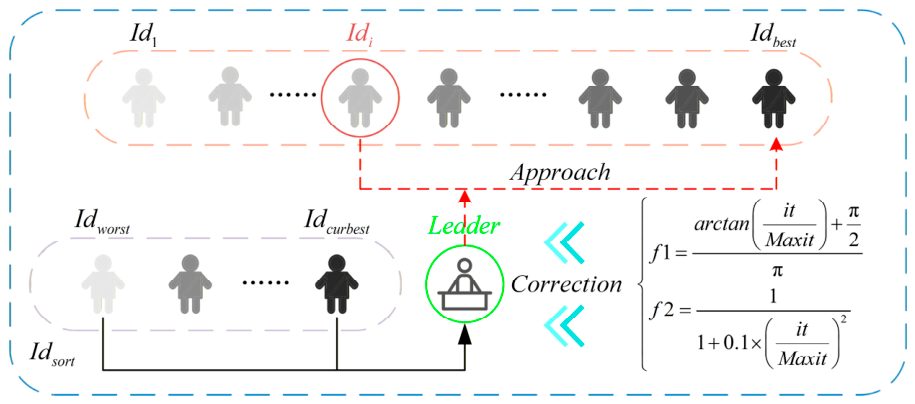
Since TLBO relies exclusively on the current best individual to guide the population update during iteration, it is prone to becoming trapped in local optima. To address this limitation, this section introduces the Bipolar Cooperative Search (BCS) module to enhance the algorithm’s ability to escape local optima. Specifically, the BCS module first identifies the best and worst individuals and calculates a dynamic step-size factor. Under the regulation of this factor, the best and worst individuals engage in cooperative learning to produce a balanced individual. This balanced individual then guides the update of the remaining individuals in the population, thereby improving the overall performance of the algorithm. The detailed guiding procedure is illustrated in Figure 1.

First, the best and worst individuals are identified using Equation (8).

$$\left\{\begin{array}{l}Ii{d}_{best}=min\left(\mathbf{I}\mathbf{i}{\mathbf{d}}_{sort}\right)\\ Ii{d}_{worst}=max\left(\mathbf{I}\mathbf{i}{\mathbf{d}}_{sort}\right)\end{array}\right.$$

(8)

where $min\left(\cdot \right)$ and $max\left(\cdot \right)$ denote the functions for taking the minimum and maximum values, respectively, and $\mathbf{I}\mathbf{i}{\mathbf{d}}_{sort}$ represents the population obtained by sorting population $\mathbf{I}\mathbf{i}\mathbf{d}$ in ascending order of fitness value.

If the position update relies solely on moving away from the worst individual or solely on approaching the best individual, the algorithm tends to converge prematurely to local optima. To balance these two update mechanisms, this section introduces an increasing step-size factor $Inpa$ and a decreasing step-size factor $Depa$, which respectively regulate the movement toward the best individual and away from the worst individual. By dynamically adjusting these two factors, the guiding process achieves a better trade-off between exploration and exploitation, thereby enhancing the algorithm’s ability to escape local optima. The increasing step-size factor and the decreasing step-size factor are calculated by the following equations.

$$\left\{\begin{array}{l}Inpa={\displaystyle \frac{arctan\left(\frac{it}{Maxit}\right)+\frac{\pi }{2}}{\pi }}\\ Depa={\displaystyle \frac{1}{1+0.1\cdot {\left(\frac{it}{Maxit}\right)}^2}}\end{array}\right.$$

(9)

Here, $it$ denotes the current iteration number, $Maxit$ represents the predefined maximum iteration number, and $arctan\left(\cdot \right)$ is the arctangent function.

Finally, by integrating the best and worst individuals obtained from Equation (8) and the step-size factors calculated via Equation (9), the guiding individual is derived using Equation (10). This guiding individual then replaces the sole best individual in the original Equation (2) to direct the update of the remaining individuals in the population. This mechanism allows individuals to more suitably absorb information from both poles of the population during iteration, thereby enhancing the diversity and adaptability of the search direction and effectively improving the algorithm’s ability to escape local optima.

$$Ii{d}_{guide}=Inpa\cdot Ii{d}_{best}-Depa\cdot Ii{d}_{worst}$$

(10)

The bipolar cooperative search and the oscillatory random mapping learning are also executed dimension-wise. For instance, the guiding individual $Ii{d}_{guide}$ is a Dim-dimensional vector, and its components are computed independently for each dimension using the corresponding components of the best and worst individuals.

After completing the position update via the Bipolar Cooperative Search module, all newly updated individuals are subjected to boundary constraint processing to confine each variable within the predefined search scope. The adopted clipping-based boundary repair is formulated as:

$$Ii{d}_i^{new}=max\left(lb,min\left(Ii{d}_i^{new},ub\right)\right)$$

(11)

here, $Ii{d}_i^{new}$ represents the i-th individual after the ITLBO update.

4.3. Oscillatory Random Mapping Learning

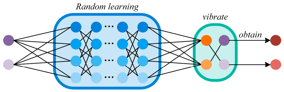
When addressing complex optimization problems, TLBO often exhibits premature convergence. The underlying cause of this issue lies in the tendency of all individuals within the population to gradually converge toward the current best individual during the iterative process, thereby rapidly diminishing population diversity. To mitigate this problem, this section introduces Oscillatory Random Mapping Learning to enhance the algorithm’s ability to maintain population diversity throughout the iterations. Specifically, the mechanism begins by randomly selecting two distinct individuals from the current population and computing the maximum and minimum values of their information across each dimension. Subsequently, the arithmetic mean of these respective maxima and minima is calculated, yielding the balanced extreme values. Following this, a designed oscillation factor, combined with the balanced extreme values, perturbs the individual positions. This introduces controlled dispersion into the newly generated population, effectively enhancing its richness and exploratory potential during the iterative process. The detailed procedure is illustrated in Figure 2.

First, two distinct individuals are randomly selected from the current population. Then, the maximum and minimum values of these two individuals across each dimension are calculated using Equation (11).

$$\left\{\begin{array}{l}{R}_{max1}=max\left(Ii{d}_{r1}\right)\\ R_{min1}=min\left(Ii{d}_{r1}\right)\\ R_{max2}=max\left(Ii{d}_{r2}\right)\\ R_{min2}=min\left(Ii{d}_{r2}\right)\end{array}\right.$$

(12)

Here, $Ii{d}_{r1}$ and $Ii{d}_{r2}$ denote two distinct individuals randomly selected from the current population. $R_{max1}$ and $R_{min1}$ represent the maximum and minimum values of individual $Ii{d}_{r1}$ across all dimensions, respectively, while $R_{max2}$ and $R_{min2}$ correspond to the maximum and minimum values of individual $Ii{d}_{r2}$, respectively. Subsequently, the balanced extreme values are calculated by fusing the maximum and minimum values of the aforementioned two random individuals using Equation (12). These balanced extreme values serve as a dynamic guiding benchmark, enabling the generation of new individuals within a reasonable range and thereby introducing more controlled random perturbations to enhance population diversity.

$$\left\{\begin{array}{l}ba{n}_{max}={\displaystyle \frac{R_{max1}+R_{max2}}{2}}\\ ba{n}_{min}={\displaystyle \frac{R_{min1}+R_{min2}}{2}}\end{array}\right.$$

(13)

Next, the oscillation factor is calculated using Equation (13). This factor is incorporated into the individual update process to introduce directed random perturbations. Specifically, the oscillation factor enables newly generated individuals to produce controlled deviations within the search space, thereby purposefully amplifying the discrepancy between them and the current best individual. This mechanism is designed to disrupt the potential clustering of individuals around the current optimum, effectively enhancing the algorithm’s global exploration capability.

$$OF=0.6+{\displaystyle \frac{1}{2}}\cdot \left(sin\left({\displaystyle \frac{it}{Maxit}}\cdot \pi -{\displaystyle \frac{\pi }{2}}\right)\right)$$

(14)

Then, by jointly utilizing the reasonable bounds defined by the balanced extreme values and the directed perturbations generated by the $OF$, a combined modulation is applied to the newly generated individual. This process systematically enhances its randomness within a controlled range, resulting in the oscillated individual $BIid$, which is specifically calculated by Equation (15).

$$BIid=OF\cdot \left(ba{n}_{min}+ba{n}_{max}-Ii{d}_i^{new}\right)$$

(15)

where $Ii{d}_i^{new}$ represents the individual after being updated by Equation (5).

Finally, to preserve the optimization trend during iterations, a greedy selection strategy is performed between individual $Ii{d}_i^{new}$ and individual $BIid$. This strategy directly compares their fitness values and retains the superior one as the individual for the new generation, thereby ensuring the algorithm consistently progresses toward improved performance throughout the search process. The specific mathematical formulation of this selection mechanism is presented in the following equation.

$$Ii{d}_i^{new}=BIidiffit\left(BIid\right)<fit\left(Ii{d}_i^{new}\right)$$

(16)

where $fit\left(BIid\right)$ and $fit\left(Ii{d}_i^{new}\right)$ denote the fitness values of individual $BIid$ and individual $Ii{d}_i^{new}$, respectively. Subsequently, the updated individual will also undergo boundary checks through Equation (11).

4.4. The Concrete Realization of ITLBO

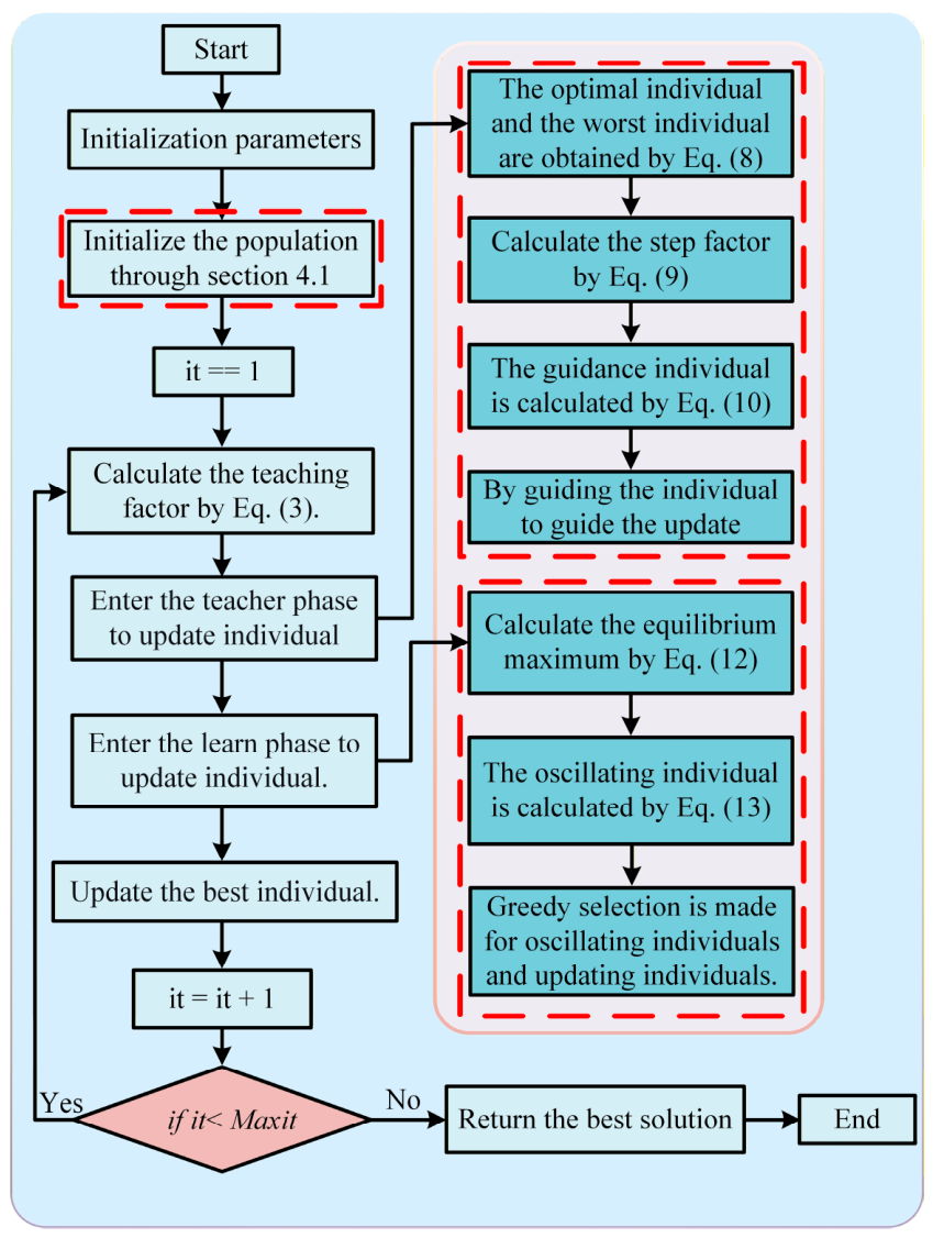
The pseudocode of ITLBO is presented in Algorithm 2, and its overall flowchart is illustrated in Figure 3. The detailed implementation proceeds as follows:

• Step 1: Initialize the algorithm parameters, including population size $Num$, problem dimension $Dim$, search space boundaries $\left[lb,ub\right]$, maximum iteration number $Maxit$, chaotic mapping parameters $para$ and $parb$, and Gaussian parameters $sigma$.
• Step 2: Generate a high-quality initial population according to the population interaction strategy.
• Step 3: Calculate the teaching factor, which adjusts the intensity of knowledge transfer in the teacher phase.
• Step 4: Compute the guiding individual using Equation (10).
• Step 5: Enter the teacher phase and update the positions of all individuals based on the guiding individual.
• Step 6: Calculate the oscillated individual via Equation (14).
• Step 7: Enter the learner phase and further update individual positions through mutual learning among individuals.
• Step 8: Perform greedy selection between the individuals updated in the teacher and learner phases and the oscillated individual, retaining the one with better fitness for the next generation.
• Step 9: Update the current global best individual.
• Step 10: If the iteration termination condition is satisfied, return the best individual; otherwise, return to Step 3.

Algorithm 2: Pseudo-code of the ITLBO algorithm

Input: Objective function: $F$, Search space: $\left[lb,ub\right]$, Population size: $Num,$ Dimension: $Dim$, chaotic mapping parameters $para$ and $parb$, and Gaussian mutation parameters $mu$ and $sigma$. Iterations: $Maxit$, and set $it=0$ Output: Global minimum: $Ii{d}_{tea}$

1: Input: $Num,Dim,lb,ub,Maxit$;

2: Use the population interaction strategy to initialize the population.

3: while $it<Maxit$ do

4:     %% Teacher stage

5:     Calculate the teaching factor by Equation (3).

6:     The guidance individual is calculated by Equation (10).

7:     Guide and update the rest of the individuals through Guide individual.

8:     Update the best individual.

9:     %% Learning stage

10:    Calculate the average position by Equation (4).

11:    The position of that individual is updated by Equation (5).

12:    The oscillating individual is calculated by Equation (14).

13:    Greedy selection of updated individuals and oscillating individuals.

14:    Update the best individual.

15: end while

16: Output: $Ii{d}_{tea}$

Most existing improved TLBO variants adopt classic metaheuristic techniques including chaotic initialization, Gaussian mutation, static best–worst guidance and separate sinusoidal perturbation in isolation or simple combination; they either use single chaotic sequences or pure Gaussian mutation without multi-population fusion and screening, employ fixed-weight or fixed-step best–worst guidance that easily leads to local optima in later iterations, or apply sinusoidal and random perturbation as independent operators unconnected with TLBO’s pairwise learning characteristics. Differing from these conventional methods, the proposed ITLBO customizes three coupled mechanisms for TLBO’s inherent two-stage framework: it integrates chaos and Gaussian mutation via population interaction for high-quality initialization, adopts dynamic adaptive best–worst guidance in bipolar cooperative search to fit the teacher phase, and embeds sinusoidal oscillation factors into TLBO’s pairwise learning rules for oscillatory random mapping learning in the learner phase.

4.5. Analysis of the Time Complexity of ITLBO

The time complexity of standard TLBO is $\mathrm{O}\left(Num\cdot Dim\cdot Maxit\right)$. The proposed ITLBO reserves the fundamental teacher-phase and learner-phase architecture of the original TLBO, and the newly added bipolar cooperative search module and oscillatory random mapping learning only increase the number of individual evaluations rather than changing the nested loop logic of the whole algorithm. Therefore, ITLBO keeps the identical time complexity of $\mathrm{O}\left(Num\cdot Dim\cdot Maxit\right)$ as conventional TLBO.

In terms of function evaluation, ITLBO requires triple function evaluations of TLBO at initialization for three-population fitness calculation. In the subsequent optimization iteration, extra search operations from two improved modules double the function evaluation quantity compared with original TLBO in each search cycle.

For memory cost and scalability, ITLBO occupies around three times the memory of original TLBO to maintain three initialized populations. Since the introduced strategies merely enrich search patterns on the original framework without altering the algorithm’s core operating logic, ITLBO maintains the same scalability as standard TLBO.

5. Experimental Analysis

In this section, we first analyze the effectiveness of the three proposed improvement strategies. Subsequently, to verify the ability of the proposed algorithm to solve complex global optimization problems, ITLBO is applied to several benchmark problems from the CEC2021 test suite for performance evaluation. Finally, a practical cloud resource scheduling problem is selected to further examine the applicability of ITLBO in real-world constrained optimization tasks. In both types of experiments, we not only compare the convergence speed and solution accuracy but also analyze the statistical stability and robustness of the results through multiple independent runs, thereby providing a comprehensive assessment of the effectiveness and practicality of the proposed strategies.

All convergence curves are derived from a single independent experimental run for each algorithm. Each data point on the curves records the best objective value found at the corresponding iteration within this standalone trial, which intuitively exhibits the real-time convergence evolution feature of each algorithm in one typical optimization process.

5.1. Effectiveness Analysis of the Proposed Strategies

In this section, the effectiveness of the Population Interaction Strategy in enhancing population diversity is first validated and analyzed. Subsequently, the role of the Bipolar Cooperative Search module and the Oscillatory Random Mapping Learning mechanism in the optimization process is examined, thereby systematically evaluating the contribution of each proposed component to the overall algorithmic performance.

5.1.1. Mechanism of Diversity Enhancement in the Population Interaction Strategy

To validate the effectiveness of the Population Interaction Strategy in improving the quality of the initial population, this paper introduces dispersion as a quantitative measure of population diversity. A higher dispersion indicates that individuals are more widely distributed across the solution space, reflecting greater exploratory potential and diversity within the population. The definition is given by the following equation.

$$Dispersion(i)=\sqrt{{\displaystyle \sum _{i=1}^{Num}{\displaystyle \sum _{j=1}^{Dim}{\left(Ii{d}_i^j-CM\left(i\right)\right)}^2}}}$$

(17)

where $Dispersion(i)$ denotes the population dispersion at the $i\text{-}th$ iteration, $Ii{d}_i^j$ represents the value of the $j\text{-}th$ dimension of the $i\text{-}th$ individual, and $CM\left(i\right)$ is the centroid at the $i\text{-}th$ iteration, which is calculated by the following equation.

$$CM\left(i\right)={\displaystyle \frac{1}{Num}}\cdot {\displaystyle \sum _{i=1}^{Num}Ii{d}_i^j}$$

(18)

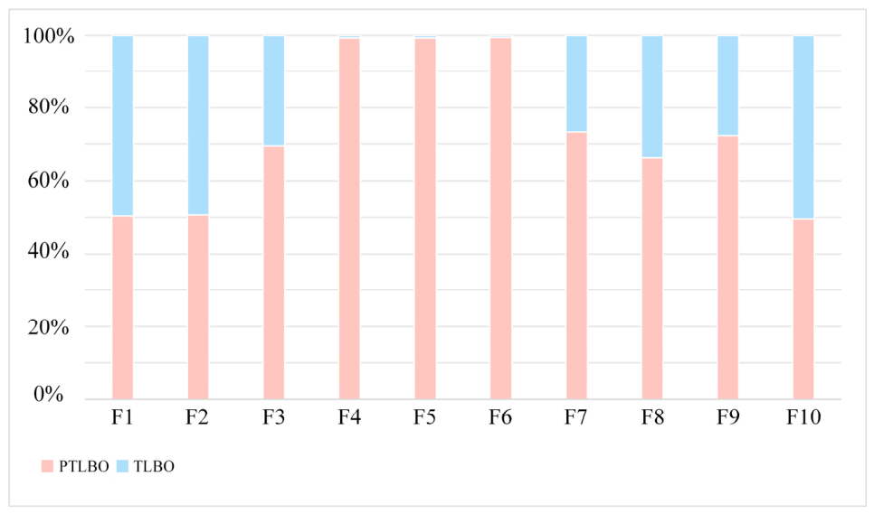
To validate the impact of the Population Interaction Strategy on the fundamental performance of the algorithm, this study conducts a comparative evaluation between a TLBO variant that incorporates only this strategy (denoted as PTLBO) and the standard TLBO using the CEC2021 benchmark set. The experimental settings are as follows: the population size is 40, the problem dimension is 20, and the maximum number of iterations is 500. All other parameters of TLBO and PTLBO are kept identical to ensure a fair comparison. The detailed specifications of the CEC2021 test suite, including function definitions and search ranges, are provided in

Table 1. Details of the CEC2021 test questions.

Index	Types	Name	Value
F1	Unimodal function	Shifted and Rotated Bent Cigar Function (CEC 2017 F1)	100
F2	Basic functions	Shifted and Rotated Schwefel’s Function (CEC 2014 F11)	1100
F3		Shifted and Rotated Lunacek bi-Rastrigin Function (CEC 2017 F7)	700
F4		Expanded Rosenbrock’s plus Griewangk’s Function (CEC 2017 f19)	1900
F5	Hybrid functions	Hybrid Function 1 ($N=3$) (CEC 2014 F17)	1700
F6		Hybrid Function 2 ($N=4$) (CEC 2017 F16)	1600
F7		Hybrid Function 3 ($N=5$) (CEC 2014 F21)	2100
F8	Composition functions	Composition Function 1 ($N=3$) (CEC 2017 F22)	2200
F9		Composition Function 2 ($N=4$) (CEC 2017 F24)	2400
F10		Composition Function 3 ($N=5$) (CEC 2017 F25)	2500
Search range: [−100, 100]

, while the convergence performance comparison of the two algorithms on each test problem is illustrated in Figure 4.

To demonstrate the effectiveness of the proposed Population Interaction Strategy, this experiment sums the population diversity values of PTLBO and TLBO for each test problem and presents the results as stacked percentage bar charts (Figure 4). The pink bars represent the percentage contributed by PTLBO’s population diversity to the total sum, while the light blue bars denote the percentage contributed by TLBO. It is evident from Figure 4 that the proportion of PTLBO exceeds that of TLBO in most test problems, directly proving that the proposed strategy effectively enhances the diversity of the initial population. On test problems F4, F5, and F6, the proportion of PTLBO’s population diversity approaches 100%, indicating its outstanding capability in maintaining diversity when solving basic and hybrid problems. On the more challenging test problems F3, F7, F8, and F9, the average proportion of PTLBO remains around 70%, further demonstrating the robust and consistent ability of the proposed strategy in enhancing population richness.

5.1.2. Search Strategy Analysis

To validate the individual and synergistic effects of the proposed strategies, this section designs the following ablation experiments. First, to examine the ability of the Bipolar Cooperative Search module to escape local optima, an algorithmic variant incorporating only this module is constructed, denoted as BSTLBO. Second, to verify the capability of Oscillatory Random Mapping Learning in mitigating premature convergence, a variant that introduces this learning mechanism is developed, labeled ORTLBO. Furthermore, to investigate the cooperative effect of the two strategies, the fully enhanced algorithm containing both is constructed, namely ITLBO. For a comprehensive evaluation, the proposed BSTLBO, ORTLBO, and ITLBO are compared with the Differential Evolution (DE) [35], Particle Swarm Optimization (PSO) [36], HOA, GWO, Whale Migration Algorithm (WMA) [37], and Artificial Lemming Algorithm (ALA) [38] on the CEC2021 benchmark set. All experiments share the following unified settings: a population size of 30, a problem dimension of 20, and a maximum iteration count of 500. Each algorithm is executed for 30 independent repeated runs to eliminate randomness of stochastic optimization. Parameters for the comparative algorithms are strictly set according to their original references to ensure fairness. The detailed comparative experimental results are presented in

Table 2. Performance comparison of different algorithms on the CEC2021 benchmark problems.

Fun	Index	DE	PSO	HOA	GWO	WMA	ALA	TLBO	BSTLBO	ORTLBO	ITLBO
F1	Mean	8.46 × 105	8.21 × 105	7.35 × 105	7.49 × 105	8.85 × 105	9.72 × 105	4.46 × 106	7.13 × 104	6.59 × 104	5.46 × 103
	Std	3.17 × 104	5.96 × 103	8.71 × 103	9.25 × 102	4.13 × 103	6.21 × 103	4.78 × 103	5.79 × 102	4.13 × 103	4.56 × 102
F2	Mean	5.21 × 104	4.68 × 104	2.89 × 104	2.89 × 104	2.89 × 104	2.89 × 104	2.89 × 104	4.31 × 103	6.84 × 103	2.57 × 103
	Std	4.25 × 103	7.13 × 103	6.92 × 102	7.86 × 104	5.27 × 102	7.32 × 103	6.15 × 102	3.82 × 102	3.95 × 103	4.25 × 102
F3	Mean	7.22 × 102	7.15 × 102	7.08 × 102	7.08 × 102	6.99 × 102	6.99 × 102	6.99 × 102	5.29 × 102	6.28 × 102	4.23 × 102
	Std	2.89 × 103	4.87 × 103	9.35 × 104	6.73 × 102	3.68 × 104	5.19 × 103	5.32 × 102	3.26 × 102	3.71 × 103	2.89 × 102
F4	Mean	9.37 × 102	9.57 × 102	9.43 × 102	9.37 × 102	9.56 × 102	9.13 × 102	9.89 × 102	8.12 × 102	8.65 × 102	7.79 × 102
	Std	5.16 × 105	8.24 × 103	5.83 × 103	8.91 × 104	6.39 × 102	8.15 × 105	7.28 × 103	4.17 × 102	4.26 × 103	5.16 × 103
F5	Mean	7.46 × 103	9.51 × 103	7.85 × 103	5.99 × 103	7.24 × 103	6.53 × 103	8.18 × 103	6.61 × 103	5.46 × 103	6.75 × 103
	Std	3.52 × 105	6.38 × 104	7.49 × 104	5.94 × 105	4.82 × 103	6.78 × 103	4.93 × 102	3.51 × 104	3.84 × 104	3.52 × 103
F6	Mean	7.33 × 109	4.35 × 108	3.86 × 109	3.33 × 109	3.86 × 109	3.78 × 109	3.79 × 109	7.51 × 109	5.33 × 109	6.72 × 109
	Std	6.37 × 105	9.15 × 104	8.26 × 103	9.72 × 104	5.74 × 105	9.03 × 102	8.16 × 103	4.53 × 104	4.39 × 103	6.37 × 104
F7	Mean	2.46 × 103	2.53 × 103	2.56 × 103	2.48 × 103	2.89 × 103	2.14 × 103	2.34 × 103	2.19 × 103	2.21 × 103	1.21 × 103
	Std	2.38 × 105	5.29 × 103	9.73 × 102	7.25 × 104	3.25 × 103	5.74 × 104	5.87 × 102	3.09 × 105	3.52 × 103	2.38 × 104
F8	Mean	7.96 × 105	1.53 × 105	1.53 × 105	8.07 × 104	1.53 × 105	8.07 × 104	8.07 × 104	8.07 × 104	4.89 × 104	4.72 × 104
	Std	4.71 × 104	7.82 × 103	6.37 × 103	8.36 × 104	5.91 × 105	7.69 × 102	6.84 × 103	3.98 × 102	4.07 × 104	4.71 × 104
F9	Mean	4.46 × 103	4.04 × 103	4.35 × 103	4.09 × 103	4.46 × 103	4.35 × 103	4.35 × 103	4.35 × 103	4.35 × 103	4.21 × 103
	Std	3.06 × 105	5.73 × 104	8.94 × 103	6.41 × 103	4.36 × 104	6.12 × 103	5.17 × 102	3.37 × 102	3.63 × 104	2.88 × 102
F10	Mean	8.46 × 103	8.02 × 103	7.68 × 103	7.76 × 103	7.76 × 103	7.76 × 103	7.76 × 103	7.76 × 103	5.46 × 103	4.51 × 103
	Std	5.82 × 104	8.67 × 102	7.68 × 103	9.38 × 102	6.18 × 102	8.54 × 104	7.73 × 104	4.31 × 102	4.19 × 103	3.54 × 103
Ave rank		8.2	6.8	5.7	4.1	6.4	3.9	5.7	4	3.1	2.3

.

In Table 2, the Mean values denote the average fitness calculated from 30 independent repeated runs for each algorithm, which intuitively reflects the overall optimization accuracy; the Std values represent the corresponding standard deviation derived from these 30 groups of results, used to quantify the stability and result fluctuation of each algorithm. All tabulated data are expressed in scientific notation with two decimal places retained after rounding the original experimental values. The last row of Table 2 lists the overall average ranking of all comparative algorithms on the entire CEC2021 test set. It can be clearly observed from the aggregated ranking results that ITLBO obtains the optimal comprehensive ranking value of 2.3 and achieves the best overall performance against all compared peer algorithms. In this table, all optimal Mean results for each test function are marked in bold for intuitive comparison. Specifically, ITLBO acquires the minimum average error and ranks first on seven out of ten CEC2021 benchmark functions, namely F1, F2, F3, F4, F7, F8, and F10, which fully verifies that the organic combination of the bipolar cooperative search module and oscillatory random mapping learning effectively upgrades the global searching capacity of the original TLBO.

Furthermore, two improved single-strategy variants, BSTLBO and ORTLBO, gain average rankings of 4.0 and 3.1, respectively, both obviously superior to the original TLBO with an average ranking of 5.7. Such statistical outcomes prove that each independent improvement strategy can effectively boost the optimization performance of basic TLBO. Notably, ORTLBO obtains the optimal average precision on F5, which is the sole test case where ITLBO fails to secure the leading position. This phenomenon demonstrates that the Oscillatory Random Mapping Learning module has unique advantages when solving hybrid optimization problems like F5 and makes irreplaceable contributions to the final performance promotion of ITLBO. From the Std, ITLBO has relatively small standard deviation values on most test functions compared with other competitors, revealing that the proposed algorithm possesses outstanding robustness and stable convergence performance across repeated optimization experiments. By contrast, conventional TLBO and several classical comparison algorithms show larger Std data on multiple benchmark problems, meaning their optimization results fluctuate violently across independent runs and lack reliable stability.

5.2. Performance Evaluation on the CEC2021

To comprehensively evaluate the capability of the proposed ITLBO algorithm in solving complex global optimization problems, this section introduces the CEC2021 standard benchmark function set, which encompasses diverse function characteristics, to systematically verify its overall optimization performance. First, the experimental environment configuration and algorithm parameter settings are described in detail. Then, the convergence accuracy and speed of ITLBO in solving various test problems are analyzed through convergence curves and statistical metrics. Finally, the robustness and stability of its optimization results are verified and further analyzed via multiple independent runs.

5.2.1. Experimental Environment and Parameter Configuration

All experiments in this paper were conducted under the Windows 11 operating system, with MATLAB R2024b serving as the computational and simulation platform. Parameters of the compared algorithms were strictly set according to their original publications. The detailed experimental configurations are as follows: in Section 5.2.2, the initial population size was set to 30, the problem dimension was 10 or 20, and the maximum number of iterations was 300.

5.2.2. Comparative Analysis of Convergence Performance

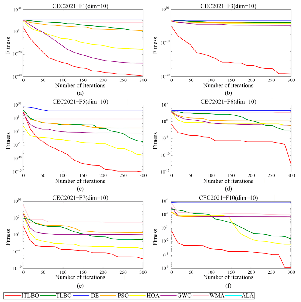
Figure 5 presents the convergence curves of the compared algorithms on six 10-dimensional CEC2021 benchmark problems (F1, F3, F5, F6, F7, and F10) in subfigures (a) through (f), respectively. The curves are distinguished by color as follows: the red line corresponds to the proposed ITLBO, the green line to TLBO, the blue line to DE, the brown line to PSO, the yellow line to HOA, the purple line to GWO, the pink line to WMA, and the cyan line to ALA.

As shown in Figure 5a, from the start to the end of the iteration, the convergence curve of ITLBO consistently remains at the bottom and is never surpassed by any other algorithm, indicating its notable superiority and stability in handling unimodal optimization problems. Furthermore, on test problem F3 corresponding to Figure 5b, ITLBO demonstrates a “substantial lead” over all compared algorithms, fully confirming its excellent convergence accuracy and efficiency in solving basic global optimization problems. In addition, the results in Figure 5c–e again show that ITLBO maintains outstanding search performance even on complex global optimization problems such as multimodal and hybrid functions; by the end of the iterations, it consistently achieves the best results, especially on problems F6 and F7, where ITLBO holds the leading position throughout the entire process. Figure 5f further highlights ITLBO’s powerful global exploration and local escape capability: around the 250th iteration, most other algorithms become trapped in local optima and stagnate, whereas ITLBO continues to improve and escape the stagnation region, ultimately obtaining a superior solution.

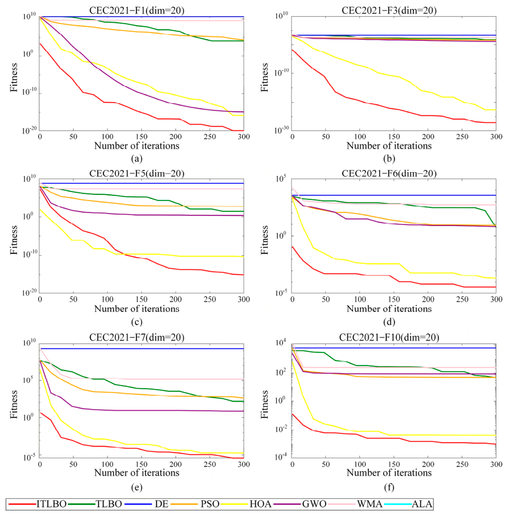
Subsequently, we scaled up the CEC2021 test problems to 20 dimensions and revalidated all compared algorithms under the same experimental settings. The results are presented in Figure 6. As shown in Figure 6a, when the dimension is increased to 20, ITLBO still maintains excellent optimization performance. Similar to the 10-Dim case, ITLBO consistently ranks first throughout the iterations. It is noteworthy that on test problems F3 and F6, TLBO, like most other algorithms, falls into local optima; in contrast, ITLBO exhibits a strong ability to escape local optima. This sufficiently demonstrates that even as the problem dimension increases, ITLBO’s capability to solve global optimization problems remains undiminished. Furthermore, on test problem F5, although HOA maintains the leading position within the first 100 iterations, ITLBO’s optimization performance surges thereafter and overtakes HOA. This indicates that as the iteration proceeds, ITLBO can effectively preserve population diversity, laying a solid foundation for the algorithm to escape local optima. In summary, the proposed ITLBO exhibits strong and robust optimization performance in solving global optimization problems.

To further quantitatively verify the optimization performance of the proposed ITLBO algorithm, comparative experiments based on the CEC2021 benchmark suite under 20-dimensional search space are carried out. The statistical indicators including the best value, mean value, worst value and standard deviation obtained by ITLBO and seven baseline metaheuristic algorithms (TLBO, DE, PSO, HOA, GWO, WMA, ALA) are summarized in

Table 3. Statistical results of various algorithms on CEC2021 benchmark functions (Dim = 20).

Fun	Index	TLBO	DE	PSO	HOA	GWO	WMA	ALA	ITLBO
F1	Best	3.72 × 105	8.91 × 1010	5.18 × 105	6.25 × 10−15	4.39 × 10−16	7.82 × 108	9.65 × 1010	2.96 × 10−20
	Mean	2.15 × 108	9.27 × 1010	3.69 × 108	5.81 × 10−4	4.92 × 10−7	8.91 × 109	9.83 × 1010	8.37 × 10−13
	Worst	6.83 × 1010	9.92 × 1010	7.91 × 1010	9.36 × 1010	9.58 × 1010	9.91 × 1010	9.99 × 1010	3.25 × 104
	Std	1.57 × 102	4.28 × 101	2.16 × 102	9.35 × 105	2.74 × 106	9.63 × 101	7.35 × 101	2.51 × 107
	p	3.25 × 10−6	7.18 × 10−7	2.69 × 10−8	5.31 × 10−6	8.27 × 10−7	4.72 × 10−6	9.13 × 10−8	\
F2	Best	8.15 × 10−6	7.21 × 10−7	3.28 × 10−5	8.15 × 10−6	2.73 × 10−6	5.92 × 10−7	4.16 × 10−5	3.15 × 10−9
	Mean	2.86 × 10−3	6.35 × 10−4	2.71 × 10−2	1.19 × 10−3	8.36 × 10−3	4.27 × 10−3	5.92 × 10−3	7.28 × 10−8
	Worst	7.92 × 10−2	5.18 × 10−3	9.35 × 10−2	6.28 × 10−3	4.15 × 10−2	2.83 × 10−2	3.76 × 10−2	2.59 × 10−2
	Std	4.17 × 102	1.29 × 103	3.82 × 102	2.15 × 104	1.53 × 103	8.16 × 103	1.09 × 102	2.16 × 104
	p	5.13 × 10−7	8.36 × 10−6	3.17 × 10−8	9.25 × 10−7	4.28 × 10−6	6.39 × 10−7	1.85 × 10−8	\
F3	Best	6.38 × 108	7.92 × 108	3.57 × 107	4.19 × 107	5.83 × 108	7.26 × 108	3.28 × 107	3.85 × 10−28
	Mean	7.19 × 108	8.35 × 108	6.92 × 107	7.38 × 10−2	7.91 × 108	8.12 × 108	6.57 × 107	8.72 × 10−20
	Worst	9.92 × 108	9.87 × 108	9.95 × 108	9.91 × 108	9.93 × 108	9.96 × 108	9.94 × 108	3.57 × 10−5
	Std	5.38 × 102	3.26 × 102	9.27 × 102	6.19 × 103	4.81 × 102	3.92 × 102	5.92 × 102	2.63 × 106
	p	2.18 × 10−6	9.27 × 10−7	4.26 × 10−9	3.52 × 10−6	8.73 × 10−7	7.15 × 10−6	5.29 × 10−8	\
F4	Best	5.36 × 108	1.83 × 105	7.29 × 109	3.75 × 106	2.81 × 107	1.27 × 105	5.82 × 108	4.82 × 104
	Mean	2.71 × 109	7.32 × 108	3.58 × 1010	1.36 × 109	2.15 × 109	5.19 × 108	3.16 × 109	1.39 × 106
	Worst	8.25 × 109	2.86 × 109	9.72 × 1010	3.27 × 109	5.39 × 109	1.83 × 109	7.92 × 109	8.25 × 107
	Std	4.83 × 102	1.25 × 103	6.18 × 102	2.71 × 102	3.82 × 102	9.36 × 103	5.27 × 102	4.12 × 103
	p	7.29 × 10−8	9.73 × 10−7	3.18 × 10−9	8.36 × 10−8	4.71 × 10−7	9.82 × 10−7	7.35 × 10−9	\
F5	Best	4.28 × 102	6.35 × 109	3.19 × 102	5.93 × 10−10	2.36 × 101	4.73 × 108	5.19 × 108	5.93 × 10−15
	Mean	2.15 × 105	7.82 × 109	6.92 × 106	1.15 × 10−6	1.82 × 103	7.13 × 108	8.16 × 108	1.72 × 10−9
	Worst	6.93 × 1010	9.92 × 109	9.36 × 108	3.16 × 102	4.71 × 108	9.92 × 108	9.95 × 108	7.36 × 108
	Std	4.17 × 103	1.27 × 102	6.15 × 103	2.35 × 105	3.58 × 102	8.26 × 102	5.83 × 102	4.96 × 107
	p	3.19 × 10−7	6.28 × 10−6	2.37 × 10−8	5.18 × 10−7	8.32 × 10−6	4.27 × 10−7	9.71 × 10−9	\
F6	Best	3.72 × 102	5.18 × 104	4.19 × 102	6.25 × 10−4	3.39 × 102	7.82 × 103	9.65 × 103	2.87 × 10−5
	Mean	2.15 × 103	7.91 × 104	9.69 × 102	5.81 × 10−1	4.92 × 103	8.91 × 104	9.83 × 104	8.53 × 10−3
	Worst	6.83 × 104	9.92 × 104	7.91 × 103	9.36 × 104	9.58 × 104	9.91 × 105	9.99 × 105	3.92 × 10−1
	Std	1.57 × 102	4.28 × 102	2.16 × 102	9.35 × 103	2.74 × 102	9.63 × 102	7.35 × 102	2.41 × 105
	p	4.72 × 10−6	8.31 × 10−7	2.92 × 10−8	6.83 × 10−6	9.17 × 10−7	5.81 × 10−6	2.36 × 10−8	\
F7	Best	4.28 × 103	6.35 × 109	3.19 × 103	5.93 × 10−4	2.36 × 101	4.73 × 105	5.19 × 105	3.72 × 10−5
	Mean	2.15 × 105	7.82 × 109	6.92 × 104	1.15 × 10−3	1.82 × 104	8.93 × 105	9.26 × 105	9.26 × 10−4
	Worst	6.93 × 108	9.92 × 109	9.36 × 108	3.16 × 108	4.71 × 108	9.92 × 105	9.95 × 105	4.15 × 101
	Std	4.17 × 102	1.27 × 102	6.15 × 102	2.35 × 104	3.58 × 105	8.26 × 102	5.83 × 102	2.73 × 103
	p	6.38 × 10−7	9.82 × 10−6	3.92 × 10−9	3.71 × 10−7	7.29 × 10−6	9.26 × 10−7	5.18 × 10−9	\
F8	Best	2.03 × 10−2	1.36 × 10−2	2.57 × 10−2	1.72 × 10−2	1.91 × 10−2	1.28 × 10−2	2.35 × 10−2	2.59 × 10−3
	Mean	2.59 × 10−2	2.15 × 10−2	3.08 × 10−2	2.43 × 10−2	2.57 × 10−2	2.01 × 10−2	2.91 × 10−2	5.92 × 10−3
	Worst	3.72 × 10−2	2.93 × 10−2	4.31 × 10−2	3.35 × 10−2	3.52 × 10−2	2.76 × 10−2	4.13 × 10−2	9.17 × 10−3
	Std	4.51 × 10−1	3.72 × 10−1	5.29 × 10−1	4.16 × 10−1	4.73 × 10−1	3.38 × 10−1	5.15 × 10−1	1.72 × 101
	p	3.72 × 10−6	7.93 × 10−7	2.51 × 10−8	8.26 × 10−6	5.39 × 10−7	9.81 × 10−6	6.37 × 10−8	\
F9	Best	7.25 × 102	3.16 × 100	1.17 × 102	6.38 × 101	5.18 × 101	2.72 × 100	8.36 × 102	3.28 × 10−1
	Mean	1.27 × 102	6.25 × 101	1.83 × 102	8.15 × 101	1.03 × 102	4.83 × 101	1.52 × 102	7.91 × 101
	Worst	2.15 × 103	1.19 × 102	2.92 × 103	1.37 × 102	1.72 × 103	8.92 × 101	2.47 × 103	2.96 × 102
	Std	2.18 × 102	9.73 × 101	3.15 × 102	1.32 × 102	1.83 × 102	8.15 × 101	2.73 × 102	2.35 × 102
	p	2.51 × 10−7	6.38 × 10−6	3.27 × 10−9	4.72 × 10−7	8.92 × 10−6	5.39 × 10−7	9.28 × 10−9	\
F10	Best	3.72 × 102	5.18 × 104	4.19 × 102	6.25 × 10−2	3.39 × 102	1.58 × 102	9.65 × 102	4.31 × 10−3
	Mean	2.15 × 103	7.91 × 104	7.69 × 102	9.81 × 10−2	4.92 × 102	8.91 × 102	9.83 × 103	9.67 × 10−2
	Worst	6.83 × 104	9.92 × 104	7.91 × 104	9.36 × 103	9.58 × 104	9.91 × 104	9.99 × 104	3.18 × 10−1
	Std	1.57 × 102	4.28 × 102	2.16 × 102	9.35 × 101	2.74 × 102	9.63 × 102	7.35 × 102	2.79 × 103
	p	9.26 × 10−8	4.18 × 10−6	2.17 × 10−9	7.15 × 10−8	3.52 × 10−6	8.29 × 10−8	5.28 × 10−9	\

. Meanwhile, the Wilcoxon rank-sum test at the significance level of 0.05 is adopted to quantify the statistical difference between ITLBO and these baseline competitors, and corresponding p-values are listed in Table 3.

As observed from the numerical data in Table 3, the designed ITLBO obtains the optimal best objective values on all ten CEC2021 test functions and exhibits obvious advantages over all selected baseline algorithms. For unimodal, multimodal and composite functions contained in CEC2021, most baseline algorithms suffer from severe premature convergence and are prone to trapping into local optima with high optimization errors, whereas ITLBO steadily decreases the fitness error and converges toward much lower objective magnitudes. In terms of mean and worst metrics, ITLBO also achieves far superior results across nearly all benchmark cases, verifying its prominent capability in global exploration and local exploitation. Moreover, ITLBO produces distinctly smaller standard deviation values relative to the baseline algorithms, which reflects its favorable robustness and stable optimization results over multiple independent runs. In accordance with Wilcoxon test outcomes, all calculated p-values are smaller than the threshold of 0.05, which statistically confirms that ITLBO achieves significant performance improvement compared with each baseline algorithm. These numerical comparisons and statistical analyses fully verify the effectiveness of the improved strategies embedded in ITLBO for balancing exploration and exploitation.

5.3. Parameter Sensitivity Analysis

To investigate the influence of core parameters on the optimization performance of the proposed ITLBO algorithm, this section performs sensitivity analysis on the chaos control parameter and Gaussian mutation factor. By setting different parameter combinations and comparing experimental outcomes, the variation law of algorithm accuracy and robustness under diverse parameter values is explored.

Table 4. Chaos parameter sensitivity analysis.

	para	0.1	0.2	0.3	0.4	0.5	0.6	0.7	0.8	0.9
parb
0.1		5.2 × 10−3	7.3 × 10−3	1.8 × 10−2	9.5 × 10−4	3.6 × 10−3	6.1 × 10−2	2.7 × 10−3	8.2 × 10−1	4.5 × 10−2
0.2		3.7 × 10−2	8.1 × 10−3	5.5 × 10−1	2.9 × 10−2	1.2 × 10−4	7.4 × 10−3	3.3 × 10−2	9.1 × 10−3	5.8 × 10−2
0.3		2.6 × 10−3	4.9 × 10−1	6.7 × 10−2	3.8 × 10−1	7.2 × 10−3	2.3 × 10−2	5.1 × 10−1	3.6 × 10−3	8.8 × 10−2
0.4		7.5 × 10−2	3.2 × 10−3	9.2 × 10−1	4.6 × 10−2	2.8 × 10−2	5.3 × 10−1	7.7 × 10−3	2.1 × 10−1	6.4 × 10−3
0.5		4.3 × 10−1	6.8 × 10−2	2.5 × 10−1	7.1 × 10−3	5.9 × 10−2	3.7 × 10−1	1.9 × 10−3	5.2 × 10−1	7.6 × 10−2
0.6		8.3 × 10−3	2.7 × 10−1	5.4 × 10−2	6.2 × 10−1	3.9 × 10−2	7.5 × 10−3	4.8 × 10−2	9.3 × 10−1	2.2 × 10−2
0.7		5.7 × 10−2	7.2 × 10−3	3.1 × 10−1	8.5 × 10−2	4.2 × 10−3	6.6 × 10−2	2.8 × 10−1	7.9 × 10−2	5.3 × 10−3
0.8		3.5 × 10−1	5.1 × 10−2	7.8 × 10−3	2.4 × 10−1	6.3 × 10−2	8.6 × 10−3	3.2 × 10−2	4.7 × 10−1	9.4 × 10−2
0.9		6.9 × 10−2	3.8 × 10−1	5.6 × 10−3	7.3 × 10−2	2.9 × 10−1	5.8 × 10−2	8.1 × 10−3	3.4 × 10−2	6.5 × 10−1

lists the optimal objective values obtained on 20-dimensional CEC2021 function F10 under different combinations of para and parb, with population size fixed as 30 and the maximum iteration set to 300. The calculated results distribute across multiple orders of magnitude ranging from 10⁻⁴ to 10⁻¹, showing irregular fluctuation with varying parameter configurations. Some adjacent parameter pairs deliver close optimization accuracy, while the combination of para = 0.2 and parb = 0.5 yields the minimal value of 1.2 × 10⁻⁴, which is obviously superior to other schemes. When para or parb is assigned an excessively small value, the algorithm lacks sufficient search perturbation and fails to escape local optima effectively. In contrast, overly large parameter values introduce excessive random disturbance and disrupt stable local exploitation, leading to noticeable accuracy degradation. After comprehensive comparison of all tested combinations, para = 0.2 and parb = 0.5 are selected as the default parameter values for subsequent numerical experiments.

After determining the optimal values of para and parb based on the sensitivity analysis results in Table 4, we further carry out the sensitivity test for the Gaussian mutation parameter following the identical experimental configurations. Differing from the previous single-function test on F10, the parametric investigation of Gaussian mutation is conducted across all ten benchmark problems from the CEC2021 test suite to comprehensively inspect its influence on algorithm performance under diverse optimization landscapes, and the corresponding experimental results are listed in

Table 5. Gaussian parameter sensitivity analysis.

	sigma	1	2	3	4	5	6	7
Fun
F1		6.52 × 10−15	8.91 × 10−18	1.72 × 10−20	3.55 × 10−17	7.38 × 10−16	2.69 × 10−15	9.43 × 10−14
F2		4.36 × 10−20	7.25 × 10−23	2.81 × 10−25	5.94 × 10−21	3.28 × 10−19	8.75 × 10−18	6.32 × 10−17
F3		7.83 × 10−22	5.27 × 10−25	3.64 × 10−28	9.12 × 10−23	4.77 × 10−21	2.86 × 10−20	7.51 × 10−19
F4		5.19 × 10−23	8.34 × 10−25	2.53 × 10−27	6.71 × 10−22	9.25 × 10−21	4.38 × 10−20	7.16 × 10−19
F5		3.75 × 10−10	6.82 × 10−13	2.96 × 10−15	7.41 × 10−12	5.39 × 10−9	8.27 × 10−8	3.61 × 10−7
F6		5.82 × 10−3	3.74 × 10−4	2.18 × 10−5	6.93 × 10−5	2.57 × 10−3	8.19 × 10−3	4.63 × 10−2
F7		7.29 × 10−3	4.51 × 10−4	2.73 × 10−5	5.86 × 10−4	3.15 × 10−3	7.52 × 10−3	5.91 × 10−3
F8		4.27 × 10−2	6.83 × 10−3	2.15 × 10−3	5.92 × 10−3	3.76 × 10−2	8.41 × 10−2	2.39 × 10−2
F9		5.93 × 10−2	7.26 × 10−3	2.68 × 10−3	6.37 × 10−3	4.29 × 10−2	9.15 × 10−2	3.82 × 10−1
F10		3.68 × 10−2	5.71 × 10−3	1.84 × 10−3	4.95 × 10−3	3.26 × 10−2	7.83 × 10−2	2.95 × 10−1

.

Table 5 records the optimal objective values of the proposed algorithm on ten CEC2021 benchmark functions when the Gaussian mutation parameter sigma varies from 1 to 7. By comparing the numerical results column by column, it can be found that each test function achieves its smallest objective value at sigma = 3. When sigma is less than 3 or greater than 3, the obtained optimal values increase obviously with irregular changes in numerical magnitude, indicating degraded optimization accuracy. Small sigma values lead to insufficient mutation disturbance and weaken the global exploration capability of the algorithm, while excessively large sigma causes excessive random variation and destroys local exploitation performance. After comprehensive comparison of all groups of experimental data, sigma = 3 is confirmed as the most appropriate parameter setting for Gaussian mutation and adopted in the following experiments.

5.4. Verification of Cloud Computing Task Scheduling Performance

To validate the capability of the proposed ITLBO algorithm in solving real-world engineering problems, this section introduces the cloud resource scheduling problem—characterized by complex constraints and multi-objective trade-offs—as an application scenario. First, the cloud computing task scheduling model is systematically presented, clarifying its optimization objectives and constraints. Then, the optimization performance and scalability of ITLBO are comprehensively evaluated by designing scheduling scenarios with different task scales. Finally, through multiple independent runs combined with statistical metrics, the fluctuation of the algorithmic results is analyzed to verify the stability and robustness of ITLBO in addressing cloud resource scheduling problems.

5.4.1. Cloud Resource Scheduling Problem Model

Suppose there are $M$ resources (tasks) to be scheduled and $N$ available virtual machine resources. The relationship between them can be represented by an $M\cdot N$ two-dimensional matrix $\mathbf{U}$, defined as follows.

$$\mathbf{U}=\left[\begin{array}{l}{u}_1^1\dots u_1^j\dots u_1^N\\ ⋮⋮⋮\\ u_i^1\dots u_i^j\dots u_i^N\\ ⋮⋮⋮\\ u_M^1\dots u_M^j\dots u_M^N\end{array}\right]$$

(19)

Here, $u_i^j$ is a binary variable (taking the value 0 or 1). When $u_i^j=1$, it indicates that the $i\text{-}th$ cloud resource (task) is assigned to the $j\text{-}th$ virtual machine; otherwise, it is not assigned. This paper assumes that each task can be allocated to only one virtual machine at any given time, and the sum of elements in each row of matrix $\mathbf{U}$ must equal 1.

To map the continuous real-number optimization results generated by ITLBO into practical cloud resource allocation schemes, a row-wise maximum-value decoding strategy is adopted to transform continuous solutions into binary assignment matrix. For each row corresponding to one independent cloud task, the position with the maximum element value is marked as 1, and all remaining entries of this row are set to 0, which ensures each task can only be assigned to one exclusive virtual machine and naturally satisfies the basic assignment constraint of scheduling problem.

Such a decoding scheme exerts dual-sided impacts on solution feasibility and algorithm search performance. On the one hand, this deterministic decoding rule fundamentally avoids illegal multi-VM occupation for single tasks and guarantees all decoded scheduling configurations are feasible. On the other hand, the fixed mapping mode restricts the effective feasible space derived from continuous search space, which subtly guides the searching preference of ITLBO and changes the practical convergence tendency during iterative optimization.

To systematically evaluate the comprehensive performance of cloud resource scheduling strategies, this paper selects time cost, load cost, monetary cost, and total cost as the core evaluation metrics. Since the total cost is the sum of the first three costs, and each sub-cost has different units and value ranges, the max–min normalization method is applied to standardize the data of each cost in order to eliminate scale effects and enable a fairer comparison of algorithmic performance. Based on the normalized data, the cost is calculated by the following equation.

$$\left\{\begin{array}{l}time={\displaystyle \frac{1}{M}}\cdot {\displaystyle \sum _{i=1}^M{\displaystyle \sum _{j=1}^N{u}_i^j\cdot \frac{C_{ti}/C_{vj}}{\underset{\forall i,j}{max}\left\{C_{ti}/C_{vj}\right\}}}}\\ load={\displaystyle \frac{1}{M}}\cdot {\displaystyle \sum _{i=1}^M{\displaystyle \sum _{j=1}^N{u}_i^j\cdot \frac{L_{ti}/L_{vj}}{\underset{\forall i,j}{max}\left\{L_{ti}/L_{vj}\right\}}}}\\ price={\displaystyle \frac{1}{M}}\cdot {\displaystyle \sum _{i=1}^M{\displaystyle \sum _{j=1}^N{u}_i^j\cdot \frac{\left(un\cdot C_{ti}\cdot R{B}_{ti}\right)/\left(C_{vj}\cdot R{B}_{vj}\right)}{\underset{\forall i,j}{max}\left\{\left(un\cdot C_{ti}\cdot R{B}_{ti}\right)/\left(C_{vj}\cdot R{B}_{vj}\right)\right\}}}}\end{array}\right.$$

(20)

where $C_{ti}$ denotes the computational resource vector required by the $i\text{-}th$ task, $C_{vj}$ represents the computational resource vector possessed by the $j\text{-}th$ virtual machine. $L_{ti}$ indicates the load demand vector of the $i\text{-}th$ task, $L_{vj}$ is the load capacity vector of the $j\text{-}th$ virtual machine. $R{B}_{ti}$ denotes the resource bandwidth demand vector of the $i\text{-}th$ task, $R{B}_{vj}$ denotes the bandwidth resource vector available on the $j\text{-}th$ virtual machine, and $un$ is a price constant set to $un=4$.

Therefore, the final optimization objective function is as follows.

$$Fi{t}_{opt}=\mathsf{\omega }1\cdot time+\mathsf{\omega }2\cdot load+\mathsf{\omega }3\cdot price$$

(21)

Here, $\mathsf{\omega }1$, $\mathsf{\omega }2$, and $\mathsf{\omega }3$ are weighting coefficients introduced to adjust the relative importance of the time cost, load cost, and monetary cost in the overall objective function. Since this study focuses primarily on verifying the comprehensive optimization performance of the algorithm rather than prioritizing any specific cost dimension, all weights are set to be equal, i.e., $\mathsf{\omega }1=\mathsf{\omega }2=\mathsf{\omega }3=1/3$.

In this cloud scheduling experiment, the time cost, load cost and price cost were integrated into a single objective function with equal weights. Since the core of this paper lies in verifying the optimization ability of the proposed ITLBO algorithm, rather than prioritizing any specific sub-objective in actual production, an equal-weight allocation method was adopted to unify multiple evaluation indicators.

5.4.2. Small-Scale Resource Scheduling Test

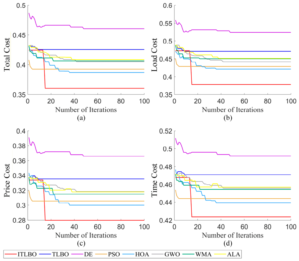
To verify the performance of ITLBO in solving cloud resource scheduling problems, this section first conducts small-scale scheduling tests. The experimental parameters are uniformly set as follows: for all compared algorithms, the population size is 30 and the maximum number of iterations is 100; the number of cloud resources (tasks) is 100, and the number of virtual machine resources is 30. The value ranges for each resource vector are: the computational resource vector of virtual machines is randomly generated within [200, 500], the load resource vector of virtual machines ranges in [100, 500], and the bandwidth resource vector of virtual machines ranges in [100, 250]; the computational resource vector of cloud tasks ranges in [10, 50], the load resource vector of cloud tasks ranges in [50, 100], and the bandwidth resource vector of cloud tasks ranges in [20, 50]. Based on the above configuration, small-scale scheduling performance tests are performed for all algorithms, and the results are shown in Figure 7.

Figure 7 illustrates the iterative processes of different algorithms in optimizing various costs for cloud resource scheduling. The curves are color-coded as follows: the red curve corresponds to ITLBO, the blue curve to TLBO, the purple curve to DE, the brown curve to PSO, the light blue curve to HOA, the gray curve to GWO, and the yellow curve to WMA. As clearly observed from Figure 7a, among all baseline algorithms, ITLBO achieves the lowest total cost for cloud resource scheduling upon the completion of iterations. Furthermore, when the iteration count reaches approximately 18, ITLBO’s optimization performance takes the lead and remains unbeaten by any other algorithm until the end of the iterations, which sufficiently demonstrates the strong capability of ITLBO in optimizing cloud resource scheduling. Moreover, in terms of load cost optimization, monetary cost optimization, and time cost optimization, ITLBO exhibits superior performance across all individual cost dimensions. Specifically, compared to the traditional TLBO, ITLBO reduces the total cost by approximately 12% in the small-scale cloud resource scheduling scenario. This finding further solidly confirms the effectiveness and superiority of the proposed ITLBO algorithm in solving real-world scheduling problems.

5.4.3. Large-Scale Resource Scheduling Test

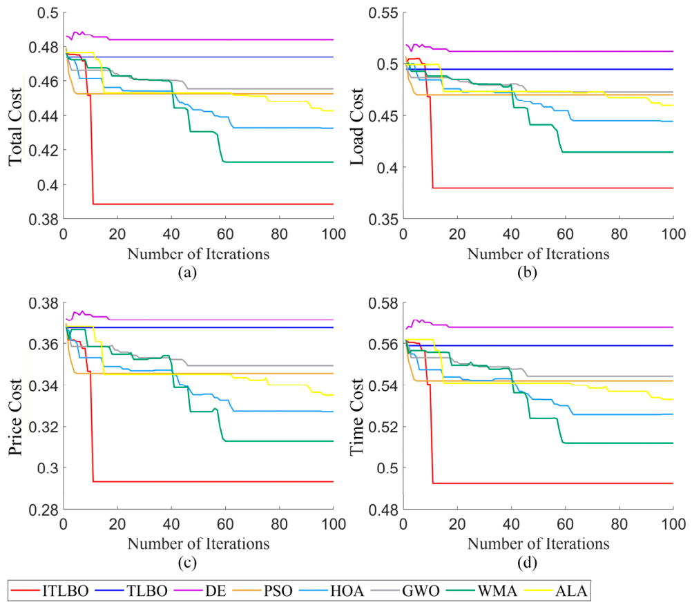
Subsequently, to verify its capability in solving large-scale cloud resource scheduling problems, this section increases the task number to 500 and adjusts the key experimental parameters accordingly: the population size is set to 40, the maximum number of iterations is 100, and the number of virtual machines is increased to 70. The value ranges for the task-related vectors are set as follows: computational resource vector [400, 1000], load vector [50, 100], and resource bandwidth vector [20, 50]; the value ranges for the virtual-machine-related vectors are set as follows: computational resource vector [1860, 2660], load vector [2048, 4096], and resource bandwidth vector [400, 500]. Under this configuration, large-scale cloud resource scheduling tests are conducted for all algorithms, and the results are presented in Figure 8.

As clearly observed from Figure 8a, ITLBO achieves the best total-cost optimization outcome among all baseline algorithms. Specifically, the total cost obtained by ITLBO is significantly lower than that of TLBO, which fully demonstrates the superior performance of the proposed strategy in optimizing large-scale cloud resource scheduling. Furthermore, from Figure 8b, it is evident that during the load-cost optimization process, TLBO remains almost entirely trapped in local optima, thereby consistently failing to obtain an efficient scheduling strategy. In contrast, ITLBO successfully escapes the local optimum after approximately 15 iterations and consistently maintains the lead thereafter. In addition, Figure 8c shows that in terms of monetary-cost optimization, ITLBO is likewise not significantly hindered by local optima and can effectively break free from stagnation early in the iterative process. In summary, for large-scale cloud resource scheduling problems, ITLBO exhibits comprehensive, efficient, and robust optimization capabilities, making it a highly competitive method for cloud resource scheduling.

5.4.4. Verification of Stability of the Scheduling Strategy

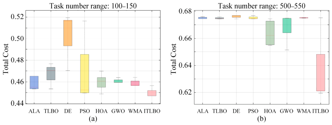
To further verify the stability of the proposed ITLBO in solving cloud resource scheduling problems, this section designs comparative experiments with different task scales. The specific parameter settings are as follows: the task number is set to the ranges [100, 150] (small scale) and [500, 550] (large scale), the population size is 30, the maximum number of iterations is 100, and the number of virtual machines is 30. The value ranges for the task-related vectors are: computational resource vector [400, 1000], load vector [50, 100], and resource bandwidth vector [20, 50]; the value ranges for the virtual-machine-related vectors are: computational resource vector [1860, 2660], load vector [2048, 4096], and resource bandwidth vector [400, 500]. Under the above settings, 100 independent runs are conducted for each compared algorithm, including ITLBO, and the total cost value of each run is recorded. Finally, box plots are drawn based on the distribution of the results from these 100 runs, as shown in Figure 9.

Figure 9a and Figure 9b present the distributions of the total cost obtained by all algorithms when the task numbers are in the ranges [100, 150] and [500, 550], respectively. From Figure 9a, it can be observed that although the height of ITLBO’s box is not the smallest, its overall range ranks the third smallest among all algorithms. This indicates that even with small-scale variations in task numbers, ITLBO maintains good optimization stability. More importantly, the upper edge of ITLBO’s box lies almost entirely below the lower edges of all other algorithms’ boxes, demonstrating that, regardless of fluctuations in task quantity, ITLBO consistently delivers superior and stable performance, which once again confirms the effectiveness of the proposed strategy. As clearly seen from Figure 9b, although the increased task scale enlarges the range of ITLBO’s box, its entire box (including the upper edge) remains positioned below the boxes of all baseline algorithms. This shows that even when the task number varies on a large scale, although the performance of ITLBO is affected to some extent, it still outperforms all baseline algorithms, sufficiently proving that ITLBO possesses strong optimization capability and robustness in solving cloud resource scheduling problems.

As summarized in

Table 6. Different algorithms have different cloud task scheduling results for different indicators.

Task Count	Index	TLBO	DE	PSO	HOA	GWO	WMA	ALA	ITLBO
100–150	Best	0.462	0.492	0.450	0.455	0.459	0.457	0.452	0.448
	Mean	0.467	0.501	0.466	0.459	0.460	0.459	0.458	0.449
	Std	1.21 × 10−3	2.75 × 10−3	3.12 × 10−3	1.03 × 10−3	0.32 × 10−3	0.89 × 10−3	1.15 × 10−3	0.97 × 10−3
	Worst	0.473	0.518	0.485	0.464	0.461	0.461	0.465	0.451
500–550	Best	0.674	0.675	0.674	0.655	0.664	0.675	0.674	0.621
	Mean	0.674	0.675	0.664	0.662	0.669	0.675	0.674	0.632
	Std	0.42 × 10−3	0.46 × 10−3	0.51 × 10−3	2.18 × 10−3	1.08 × 10−3	0.33 × 10−3	0.37 × 10−3	2.95 × 10−3
	Worst	0.675	0.676	0.675	0.672	0.675	0.675	0.675	0.649

, ITLBO achieves the most competitive best and mean results across both light and heavy task scheduling environments compared with all baseline competitors. In the low-load task scenario with fewer tasks, most baseline algorithms yield notably higher optimization values, which implies that these peer methods are easily trapped in a local optimum and fail to explore high-quality resource allocation schemes. From the standard deviation, which reflects algorithm stability, ITLBO presents mild numerical fluctuation and preferable robustness under small-scale scheduling conditions.

With the expansion of task quantity to the high-load range, the overall optimization cost of all tested algorithms rises naturally as scheduling constraints and resource matching difficulty increase sharply. Even in such complex scheduling circumstances, ITLBO still maintains dominant advantages on core statistical indicators over contrasted methods. Several baseline algorithms suffer obvious performance deterioration accompanied by sharp increases in worst objective values and large result volatility, revealing their weak adaptability when coping with complicated heavy-load scheduling problems.

Consistent with the distribution characteristics shown in the corresponding boxplots, the statistical data in Table 6 fully demonstrates that the improved strategies inside ITLBO effectively balance global exploration and local exploitation. The proposed optimizer possesses strong environmental adaptability and can steadily generate high-quality scheduling solutions under varying cloud task loads.

5.4.5. Cost Weight Sensitivity Analysis

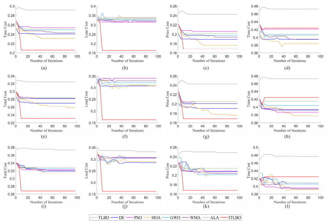
As illustrated in Figure 10, subfigures a–d present the optimization results under configuration W₁ = [0.75, 0.15, 0.15], where time cost is assigned the dominant weight, simulating delay-sensitive cloud scheduling scenarios that attach great importance to task completion efficiency. Subfigures e–h correspond to W₂ = [0.5, 0.25, 0.25], implementing a moderate balanced weight allocation for three evaluation terms and representing conventional general-purpose cloud batch scheduling tasks. Subfigures i–l show the outcomes under W₃ = [0.2, 0.4, 0.4], with load cost and price cost set as dominant optimization targets, fitting resource-conservation-oriented scheduling scenes focusing on server load balance and economic overhead control. Identical experimental parameters are adopted across all test cases: the total number of scheduling tasks is fixed at 100, the available virtual resource node quantity is set as 40, the maximum iteration number is 100, and the population size of all optimization algorithms is uniformly set to 30. In terms of initialization ranges, virtual machine-related parameters are restricted within specified intervals, where computing resource varies from 200 to 500, load parameter ranges from 100 to 500 and bandwidth is limited between 100 and 150. Meanwhile, relevant property parameters of scheduling tasks are initialized with computing demand from 10 to 50, task load from 50 to 100 and required bandwidth from 20 to 50. The color coding for all algorithms remains consistent across the whole figure: gray curves denote TLBO, light green curves represent ALA, dark blue curves stand for DE, purple curves indicate PSO, tan curves correspond to HOA, light blue curves signify GWO, indigo curves refer to WMA, and red curves illustrate the proposed ITLBO.

Across all three weight scenarios, ITLBO consistently outperforms the compared baseline algorithms in both convergence speed and final optimization performance. Specifically, ITLBO exhibits the steepest decline in total cost during the early iterations, typically converging to favorable near-optimal solutions within 20–40 iterations, whereas baseline algorithms such as TLBO and PSO demonstrate considerably slower convergence trajectories and frequently plateau at obvious suboptimal levels. In the time-cost-prioritized scenario defined by W₁, ITLBO yields the optimal load cost and economic cost compared with all peer algorithms. Such results guarantee acceptable task latency and bring outstanding optimization on the remaining core indicators for efficiency-oriented cloud tasks. Under the moderate balanced-weight configuration of W₂, ITLBO achieves prominent overall reduction on total scheduling cost without triggering severe deterioration in any single sub-objective, underscoring its capacity to find well-balanced resource allocation schemes. When load and price costs are prioritized under W₃, ITLBO attains the lowest load and price cost values while preserving reasonable control over time expenditure, thereby realizing excellent resource economy and load balancing performance. A particularly noteworthy characteristic of ITLBO is its adaptive optimization behavior in response to weight variations. When the weight of a specific objective is increased, ITLBO exhibits a stronger optimization tendency toward that target via its embedded improved search strategies, yet it successfully avoids causing severe degradation in other evaluation metrics. The algorithm’s enhanced global exploration and refined local exploitation mechanisms enable it to handle the complex trade-off relationship among conflicting scheduling objectives without falling into local optima prematurely. In contrast, several baseline algorithms demonstrate unstable or even poor performance under certain weight configurations. For instance, TLBO frequently exhibits obvious premature convergence across three weight groups, failing to continuously search for high-quality scheduling solutions. PSO shows severe oscillatory behavior on load and price cost optimization under multiple weight settings, indicating its insufficient adaptability toward changing objective preference. GWO and DE occasionally achieve competitive results on individual single indicators but struggle to maintain steady and superior comprehensive performance across all objectives simultaneously. ALA and WMA deliver moderate optimization results in partial cases but lack the multi-strategy enhancement to adapt flexibly to diversified weighted scheduling requirements.

6. Conclusions

This paper proposes an ITLBO designed to effectively tackle complex problems such as global optimization and cloud resource scheduling. Specifically, by incorporating the Population Interaction Strategy, the diversity of the initial population is enhanced, thereby improving the accuracy of the final solution. The introduction of the Bipolar Cooperative Search module strengthens the algorithm’s ability to escape local optima, consequently accelerating convergence speed. Furthermore, the integration of Oscillatory Random Mapping Learning dynamically maintains population diversity during the iterative process, effectively mitigating premature convergence. Experimental results on the CEC2021 benchmark functions and cloud resource scheduling scenarios demonstrate that ITLBO exhibits notable advantages in both optimization performance and robustness.