


Abstract
Objective diagnosis in psychiatry remains challenging due to the lack of reliable biological markers and the presence of confounding variables in observational data. While EEG-based machine learning models have shown promising classification performance, their validity remains unclear when confounding factors such as age are not explicitly controlled. In this work, we propose a confound-aware mathematical framework for supervised learning, where classification is formulated as a mapping under the presence of a confounding variable A. Within this formulation, model performance is interpreted as a function of both predictive structure and confound dependence. The proposed framework integrates classification, regression, and feature selection into a unified evaluation pipeline. A central contribution is the Cross-Task Explanation Concordance (CTEC) index, a rank-based metric that quantifies the stability of feature importance across models and predictive tasks. Experimental results on a large-scale EEG dataset (N = 670) demonstrate that deep learning models outperform handcrafted approaches under standard evaluation. However, under confound-controlled settings, handcrafted models show a dual response to confound control: age residualization improves classification by removing feature-level noise (+20.3%), while age-matching collapses performance to chance (balanced accuracy, BA = 0.238) by eliminating demographic separability. Deep learning models retain partial robustness under both conditions. These findings highlight that conventional performance metrics may overestimate model validity in the presence of structured bias. The proposed framework provides a general mathematical approach for evaluating supervised learning models under confounding effects and is applicable to a wide range of data-driven systems beyond EEG.
Keywords:
EEG; explainable AI; psychiatric classification; brain-age; SHAP; EEGConformer; cross-task concordance; age confound; TDBRAIN MSC:
68T07
1. Introduction
Mental health disorders represent a leading cause of global disability, affecting approximately one billion people worldwide [1]. Clinical diagnosis currently relies on subjective interviews and self-report instruments guided by the Diagnostic and Statistical Manual of Mental Disorders (DSM-5) [2], a process that is time-consuming, prone to inter-rater variability, and lacks objective biological grounding [3]. The development of computational tools that can assist clinicians with objective, brain-based diagnostic support remains a critical unmet need in psychiatry. However, despite increasing use of EEG-based machine learning approaches, it remains unclear whether reported classification performance reflects disorder-specific neural signatures or is driven by confounding factors such as age.
Despite rapid progress in EEG-based machine learning, a critical gap remains between reported model performance and clinical validity. Many studies achieve high accuracy under experimental conditions but fail to account for confounding variables, particularly age, which strongly influences EEG characteristics. As a result, it remains unclear whether these models capture disorder-specific neural signatures or merely reflect demographic structure.
Electroencephalography (EEG) is uniquely positioned to address this need due to its non-invasive nature, low cost, high temporal resolution (millisecond scale), and widespread clinical availability [4]. Unlike functional MRI, EEG equipment is portable, relatively inexpensive, and can be administered in routine clinical settings. Resting-state EEG, in which participants sit quietly with eyes open or closed for several minutes, is particularly attractive for clinical deployment because it requires no task compliance and is feasible across age groups, cognitive abilities, and severity levels [5]. However, EEG spectral and temporal characteristics are strongly influenced by demographic factors, particularly age, raising concerns that learned models may capture population structure rather than diagnosis-specific neural information.
This limitation raises critical concerns regarding the interpretability and clinical reliability of EEG-based biomarkers, especially when models are evaluated without explicit control of demographic confounds.
Recent advances in machine learning and deep learning have demonstrated that EEG signals contain information relevant to psychiatric diagnosis [6,7]. However, the existing literature suffers from several critical limitations that impede clinical translation. First, the vast majority of studies employ binary classification (one disorder versus healthy controls), which does not reflect the clinical reality where clinicians must differentiate among multiple disorders with overlapping symptom profiles [8]. Second, many studies report inflated accuracies from small samples (N < 100) using within-subject or within-session evaluation paradigms that overestimate generalization performance [9]. Third, most studies lack systematic explainability analysis; when explanations are provided, they are limited to a single model and a single task, making it difficult to assess whether identified biomarkers are robust across analytical perspectives [10]. More critically, existing studies do not evaluate whether identified biomarkers remain consistent across different models and predictive tasks, making it unclear whether reported findings reflect stable neurophysiological signatures or model-specific artifacts.
From a methodological perspective, these limitations indicate that model evaluation is often treated as a purely predictive problem, without formally accounting for the influence of confounding variables on the learned mapping. Collectively, these limitations highlight a broader methodological issue: current EEG-based psychiatric models are predominantly evaluated under performance-driven criteria, with insufficient emphasis on robustness, interpretability, and cross-context validation.
A particularly underappreciated challenge is the role of demographic confounds, especially age. Psychiatric disorders exhibit characteristic age-of-onset distributions (e.g., ADHD in childhood, depression in midlife, cognitive complaints in aging), and EEG spectral characteristics change substantially with age [11]. Without explicit age-controlled analysis, a classifier may achieve above-chance accuracy by exploiting age-related spectral differences rather than genuine diagnosis-specific biomarkers, a critical limitation that few studies address [11]. This raises a fundamental validity question: can EEG-based classifiers distinguish psychiatric conditions independently of age, or do they primarily capture age-related spectral differences?
In this context, the observed classification performance may reflect not only the relationship between EEG signals and diagnostic labels but also the influence of confounding variables such as age. Addressing this question is essential for establishing EEG-based models as clinically meaningful tools rather than statistical predictors driven by dataset biases.
To address these gaps, this study introduces a three-pillar explainable AI framework that simultaneously tackles three complementary clinical questions: (1) Can resting-state EEG distinguish between five psychiatric conditions? (2) Can EEG predict brain age, and does the brain-age gap differ across diagnoses? (3) Can a minimal set of features support clinical screening? Critically, we propose the Cross-Task Explanation Concordance (CTEC) index, a novel metric that quantifies the consistency of feature importance across models and predictive tasks. Unlike existing approaches, the framework explicitly incorporates confound-aware evaluation. This enables model performance to be interpreted in the context of confound sensitivity rather than as a standalone metric.
We evaluate three model families representing different analytical paradigms: XGBoost [12] on handcrafted spectral, connectivity, and nonlinear EEG features; EEGNet [13], a compact convolutional neural network designed for EEG; and EEGConformer [14], a hybrid CNN–Transformer architecture that captures both local and global temporal dependencies. All models are compared under controlled conditions using the TDBRAIN dataset [15], a large single-site resting-state EEG database spanning two decades of clinical recordings. The overall study framework is illustrated in Figure 1. Importantly, all models are evaluated under participant-level cross-validation and multiple confound-controlled settings to ensure a fair and clinically meaningful comparison.
Figure 1.
Study framework overview. The proposed three-pillar explainable AI framework comprises multi-class psychiatric classification (Pillar 1), brain-age regression (Pillar 2), and minimal-feature screening (Pillar 3), applied to the TDBRAIN dataset (N = 670, 26-channel resting-state EEG). Three model families are evaluated: XGBoost on 2397 handcrafted features, EEGNet (compact CNN), and EEGConformer (CNN–Transformer hybrid) on raw EEG signals. The explainable AI layer applies TreeSHAP to XGBoost and Integrated Gradients (IG) to deep learning models. The Cross-Task Explanation Concordance (CTEC) index quantifies agreement across tasks and models (composite = 0.563). Age confound validation demonstrates that deep learning retains diagnostic signal (EEGNet: BA = 0.336, 1.34× chance) while handcrafted features drop to chance under age-matching. EO: eyes open; EC: eyes closed; BAG: brain-age gap; WTS: within-task stability; CMA: cross-model agreement.
The contributions of this work are 4-fold. First, we present a systematic participant-level evaluation of multi-class EEG classification under explicit demographic confound analysis using the TDBRAIN dataset. Second, we introduce the Cross-Task Explanation Concordance (CTEC) framework to quantify the stability and agreement of feature attribution patterns across predictive tasks and model families. Third, we compare handcrafted-feature learning and end-to-end deep learning under multiple confound-controlled settings, including feature residualization, age-matched evaluation, and restricted age-range analysis. Finally, we demonstrate that although deep learning models consistently outperform handcrafted approaches, classification performance remains strongly influenced by demographic structure. These findings highlight the importance of confound-aware validation for clinically meaningful EEG biomarkers. Rather than focusing solely on predictive accuracy, the proposed framework emphasizes robustness, interpretability, and validity-driven evaluation. The primary novelty of this work is not the individual predictive tasks themselves, but the integration of classification, regression, confound analysis, and explanation concordance within a unified confound-aware evaluation framework.
2. Related Work
2.1. EEG-Based Psychiatric Classification
The application of machine learning to EEG-based psychiatric diagnosis has grown rapidly over the past decade, with studies spanning depression [16], ADHD [17,18,19], schizophrenia [5,20], and other conditions. A recent systematic review by Craik et al. [6] identified depression, epilepsy, and Alzheimer’s disease as the most studied conditions, with reported accuracies ranging from 70% to above 99%. However, these high accuracies are predominantly from binary classification with small samples (often N < 50 per class), raising serious concerns about generalizability and clinical relevance [9]. Importantly, many of these reported performances are derived from experimental settings that do not reflect real-world clinical scenarios, where multiple disorders must be distinguished simultaneously and data distributions are highly heterogeneous.
Multi-class psychiatric classification from EEG remains underexplored. Park et al. [8] classified six psychiatric categories from resting-state quantitative EEG (QEEG) in 945 participants, achieving per-disorder accuracies of 74–94% in binary settings but substantially lower multi-class performance. On the TDBRAIN dataset specifically, Greiner and Zhang [21] used a Transformer architecture to classify five disorders from raw EEG, achieving window-level accuracies of 63–66%. Recently, foundation models like LaBraM [22] and BIOT [23] have shown promise for cross-dataset EEG transfer learning, though psychiatric classification remains challenging. However, a key limitation of existing studies on TDBRAIN is the reliance on window-level evaluation, which can artificially inflate performance due to multiple correlated samples per participant, thereby overestimating generalization capability.
Deep learning architectures have evolved from EEGNet [13] to increasingly sophisticated attention-based models including EEGConformer [14], ATCNet [24], and SPaRCNet [25]. Despite these architectural advances, the question of whether these models learn genuine diagnostic patterns or exploit demographic confounds remains largely unaddressed in the literature. Thus, while architectural innovation has been a primary focus of prior work, methodological rigor in validation, particularly with respect to confound control and participant-level evaluation, remains insufficient.
2.2. Brain-Age Prediction from EEG
Brain-age prediction estimates a person’s age from neuroimaging data; the difference between predicted and chronological age (the brain-age gap, BAG) serves as a biomarker for accelerated or decelerated brain aging [26]. While most brain-age research uses structural MRI [27], EEG-based approaches have gained traction. Duan et al. [28] established a reusable benchmark for M/EEG brain-age prediction, reporting MAE values of 7–10 years depending on the recording setup. Kounios et al. [29] further demonstrated that competitive brain-age estimation is achievable using consumer-grade, low-cost EEG hardware, substantially broadening the practical accessibility of EEG-based aging biomarkers beyond clinical-grade systems. Han et al. [30] reported brain-age associations with depression severity using MRI.
Despite these advances, EEG-based brain-age studies have largely been conducted in isolation from diagnostic classification tasks, limiting understanding of whether age-related representations overlap with disease-related biomarkers. Moreover, few studies explicitly investigate whether brain-age prediction introduces or reinforces confounding effects in downstream classification models, an issue particularly relevant in psychiatric datasets with skewed age distributions.
2.3. Explainable AI for EEG
Explainability in EEG classification has primarily relied on feature importance from tree-based models (via SHAP [31] or permutation importance) or saliency maps from neural networks. For deep learning, Integrated Gradients [32], Grad-CAM [33], and attention weight visualization are commonly used. Sturm et al. [34] applied layer-wise relevance propagation (LRP) to EEG deep learning, while Borra et al. [35] compared multiple XAI methods for EEG decoding. Tjoa and Guan [36] provided a comprehensive survey of medical XAI. Existing explainability approaches are typically applied to a single model or predictive task [37], limiting assessment of explanation stability across analytical contexts. Moreover, no prior study has systematically evaluated whether explanations remain consistent across different model architectures and predictive objectives (e.g., classification versus regression). This limits assessment of the robustness of identified biomarkers. This gap motivates our CTEC index. The present work addresses this limitation by introducing a unified evaluation framework that explicitly quantifies explanation consistency across tasks, models, and validation conditions, thereby advancing the methodological rigor of XAI in EEG research.
3. Materials and Methods
3.1. Problem Formulation
We consider a supervised learning problem defined over a dataset of samples:
where represents the EEG signal, is the class label, and denotes a confounding variable (e.g., age). The goal is to learn a mapping:
such that
We assume a joint data distribution:
Which explicitly models the dependence between the input signal, the target label, and the confounding variable, thereby extending standard supervised learning formulations to a confound-aware setting. In the presence of confounding,
This inequality indicates that the predictive relationship between EEG signals and labels is not independent of the confound, implying that a model may exploit confounding structure to achieve artificially inflated performance. We define the expected predictive performance as
where denotes a bounded per-sample performance score for which higher values indicate better predictions (for example, the indicator of correct classification, whose expectation under class-balanced evaluation is the balanced accuracy). Accordingly, Perf is an expected performance rather than an expected loss. To assess the influence of confounding, we consider a confound-controlled distribution, , in which the dependence between and is reduced while preserving the structure of . The corresponding performance is defined as
We then define the confound sensitivity as
This quantity measures the extent to which model performance depends on confounding information. Because Perf is a performance score, can be positive or negative depending on whether confound control removes an exploitable shortcut or removes nuisance variance. A positive value indicates performance decreases after confound control, whereas a negative value indicates that performance improves after removing confound-related noise.
3.2. Dataset
We use the Two Decades Brainclinics Research Archive for Insights in Neurophysiology (TDBRAIN) [15], a clinical resting-state EEG database collected between 2001 and 2021 at a single EEG laboratory in The Netherlands. The full database contains 1274 participants aged 5–89 years with various psychiatric and neurological conditions. After applying inclusion criteria (session 1, DISCOVERY subset, single primary indication), our analysis cohort comprises N = 670 participants across five diagnostic classes: major depressive disorder (MDD, N = 308), attention-deficit/hyperactivity disorder (ADHD, N = 192), subjective memory complaints (SMC, N = 86), healthy controls (HC, N = 47), and obsessive–compulsive disorder (OCD, N = 37).
To ensure reproducibility and reduce selection bias, all inclusion and exclusion criteria were predefined prior to model development, and no post hoc filtering based on model performance was applied.
EEG was recorded using 26 Ag/AgCl electrodes in the international 10–10 system at 500 Hz with DC recording. Additional channels included EOG (4 channels), ECG (1 channel), and EMG (2 channels). Each participant completed a 2 min eyes-open (EO) resting-state recording followed by a 2 min eyes-closed (EC) recording. The cohort demographics are shown in Figure 2. Importantly, all analyses were conducted at the participant level, ensuring that no data from the same participant appeared in both training and testing sets, thereby preventing data leakage.
Figure 2.
Cohort demographics and class distribution. (a) Number of participants per diagnostic class; dashed line indicates equal class size (the expected count per class under a balanced design, N/5 ≈ 134). (b) Age distribution by diagnosis (violin plots); white stars show group means. Note the age confound: ADHD mean = 23 yr, SMC mean = 65 yr. (c) Gender distribution. MDD: major depressive disorder; ADHD: attention-deficit/hyperactivity disorder; SMC: subjective memory complaints; HC: healthy controls; OCD: obsessive–compulsive disorder.
3.3. EEG Preprocessing
Preprocessing was performed using MNE-Python 1.7.1 [38] with the following automated pipeline: (1) 50 Hz notch filtering to remove power line noise; (2) bandpass filtering (0.5–45 Hz for the main signal, 1–100 Hz for the ICA copy); (3) automated bad channel detection based on variance (z > 5), kurtosis (z > 3), and inter-channel correlation (r < 0.4) with spherical spline interpolation; (4) common average re-referencing; (5) ICA decomposition (extended Infomax, 20 components) with ICLabel [39] automated artifact classification (rejection threshold 0.60 for eye, muscle, heart, line noise, and channel noise components); (6) segmentation into 2 s non-overlapping epochs; and (7) peak-to-peak amplitude rejection (200 μV threshold) and variance-based outlier removal (z > 4). A minimum of 30 clean epochs was required per recording. Preprocessing quality-control metrics across all retained recordings are summarized in Figure 3.
Figure 3.
Preprocessing quality control metrics across 1340 successfully processed EEG recordings. (a) Epoch retention rate (mean = 98.6%), indicating minimal data loss during artifact rejection. (b) Number of ICA components removed per recording by ICLabel (mean = 3.5). (c) Individual alpha frequency distribution (mean = 9.5 Hz), validating preservation of the expected neurophysiological alpha peak. Dashed red lines indicate means; the solid black line in (c) marks the expected 10 Hz reference.
All preprocessing steps were applied uniformly across the dataset using a fully automated pipeline to eliminate manual intervention and ensure consistency across participants. No class-specific preprocessing or filtering was performed, preventing the introduction of implicit label-dependent bias.
3.4. Feature Extraction
From preprocessed epochs, we extracted 2397 features organized into five complementary views (Figure 4). The multi-view feature design was intentionally constructed to capture complementary aspects of EEG dynamics, including spectral, spatial, and nonlinear properties, thereby reducing the risk of relying on a single feature domain.
Figure 4.
Feature extraction views and inter-view relationships. (a) Number of features per view, totaling 2397 features after quality filtering. (b) Pairwise Pearson correlation between view-averaged feature values, showing low inter-view correlations (|r| ≤ 0.30), supporting the complementarity of the multi-view design. EO: eyes open; EC: eyes closed; dwPLI: debiased weighted phase lag index.
- View 1, Spectral Power (N = 754): Absolute and relative power spectral density in six frequency bands (delta: 1–4 Hz, theta: 4–8 Hz, alpha: 8–13 Hz, low beta: 13–20 Hz, high beta: 20–30 Hz, gamma: 30–45 Hz) [40] computed per channel and per brain region using Welch’s method with 2 s Hanning windows (50% overlap). The relative power in frequency band b for channel c was computed aswhere is the absolute band power and denotes the number of frequency bands.
- View 2, Spectral Shape (N = 258): Individual alpha frequency (IAF), aperiodic spectral slope and offset via the FOOOF algorithm [41], theta/beta ratio, and alpha asymmetry indices. Alpha asymmetry between electrode pairs was computed aswhere and denote right- and left-hemisphere alpha (8–13 Hz) power, respectively.
- View 3, Connectivity (N = 36): Functional connectivity was quantified using the debiased weighted phase lag index (dwPLI) [42] averaged across 15 region pairs in six frequency bands:where denotes the cross-spectral density between channels and .
- View 4, Nonlinear Dynamics (N = 248): Sample entropy, Lempel–Ziv complexity, Higuchi fractal dimension, and detrended fluctuation analysis per channel and per region. Sample entropy was computed aswhere is the count of template matches of length within tolerance , and is the count of matches of length , using and .
- View 5, EO-EC Reactivity (N = 1101): Differences and ratios between eyes-open and eyes-closed conditions for all features in Views 1–4.
All features were computed independently for each participant and then aggregated across epochs to ensure that the resulting feature representation reflects stable subject-level characteristics.
3.5. Classification Models
Each preprocessed EEG recording was represented as a tensor:
where is the number of epochs, is the number of EEG channels, and is the number of time samples per epoch (2 s at 500 Hz). Channel-wise z-score normalization was applied:
where and are the per-channel mean and standard deviation across time, and . Normalization parameters were computed exclusively on the training set within each fold and applied to the corresponding test set to prevent information leakage.
We evaluated three model families in a systematic ablation design:
- XGBoost served as the interpretable baseline, operating on the full 2397-dimensional feature vector with class-weighted sampling to address imbalance [12].
- EEGNet is a compact CNN designed for EEG with approximately 2500 parameters, comprising temporal convolution (kernel size 64), depthwise spatial convolution, and separable convolution blocks with batch normalization and ELU activation [13].
- EEGConformer (inspired by Song et al. [14]) extends the CNN approach with a two-layer Transformer encoder that applies multi-head self-attention (four heads) to temporal patch embeddings extracted by the convolutional front-end, enabling capture of long-range dependencies that local convolutions miss.
The selected model families represent three distinct learning paradigms: handcrafted feature-based learning, compact convolutional neural networks, and hybrid attention-based architectures. This design enables a direct comparison between explicit feature engineering and end-to-end representation learning, providing insight into their ability to capture discriminative EEG patterns.
Deep learning models were trained using a set of stochastic data augmentation techniques to improve generalization and robustness. Specifically, for an input signal , augmented samples were generated via
- Additive Gaussian noise with ,
- Temporal shifts within a window of ,
- Random channel dropout with probability ,
- Amplitude scaling , where .
These transformations are label-preserving and are intended to approximate realistic variability in EEG acquisition, thereby reducing overfitting to subject-specific or recording-specific artifacts.
Model optimization was performed using a class-weighted cross-entropy loss defined as
where denotes the one-hot encoded ground-truth label, is the predicted class probability, and is the inverse class-frequency weight for class , with denoting the number of samples in class . This weighting scheme compensates for class imbalance and ensures that minority classes contribute proportionally to the optimization objective. As an alternative objective, focal loss was evaluated to further address class imbalance and hard-example learning [43]:
where is the focusing parameter. The multiplicative term dynamically downweights well-classified samples and emphasizes difficult examples, thereby modifying the effective loss landscape. Training was performed using the AdamW optimizer with decoupled weight decay [44], combined with cosine annealing learning rate scheduling, gradient clipping with maximum norm equal to 1.0, and early stopping based on validation performance (patience = 20 epochs). These optimization strategies were selected to stabilize training and improve convergence in high-dimensional non-convex settings typical of deep neural networks. To obtain subject-level predictions, epoch-level outputs were aggregated using mean probability pooling. For a participant with epochs, the aggregated prediction vector is defined as
and the final predicted label is
This aggregation scheme ensures that predictions reflect subject-level characteristics rather than individual epoch fluctuations, thereby aligning the evaluation protocol with the clinical decision-making setting. A systematic ablation study was conducted to isolate the contribution of key design choices, including (i) eyes-open (EO) input versus combined eyes-open and eyes-closed (EO + EC) input, (ii) training with and without data augmentation, (iii) cross-entropy versus focal loss, and (iv) ensemble modeling via probability averaging of EEGNet and EEGConformer outputs. This controlled experimental design enables attribution of performance gains to specific architectural and training components rather than confounded interactions. All hyperparameters were selected a priori based on the established literature and fixed prior to cross-validation. Importantly, no hyperparameter tuning was performed on the test folds, and no external validation dataset was used, ensuring that the reported results represent unbiased estimates of generalization performance.
3.6. Brain-Age Regression
Brain-age estimation was formulated as a supervised regression problem using the same feature space described in Section 3.4. Let denote the chronological age of participant and denote the predicted age obtained from a regression model . The brain-age gap (BAG) is defined as
This quantity captures deviations from normative aging trajectories and is commonly interpreted as an indicator of accelerated or delayed neurophysiological aging. The regression model was implemented using XGBoost with 5-fold age-stratified cross-validation. Age stratification ensures that each fold preserves the marginal distribution of age, thereby reducing variance in performance estimates and preventing bias toward specific age ranges. Statistical comparison of BAG across diagnostic groups was performed using the Kruskal–Wallis test, followed by pairwise Mann–Whitney U tests with multiple-comparison correction. This non-parametric framework was selected due to the non-Gaussian distribution of BAG values and the presence of heteroscedasticity across groups.
3.7. Minimal-Feature Screening
To evaluate the feasibility of simplified clinical deployment, we considered a reduced feature selection framework based on model-derived importance scores. Let denote the full feature set and denote the subset of top- features selected according to
where is the mean absolute SHAP value for feature . This ranking strategy ensures that selected features reflect global model importance rather than fold-specific artifacts. Classification models (logistic regression and XGBoost) were then trained on , with . Feature selection was performed strictly within training folds to avoid information leakage, preserving the validity of the evaluation protocol.
3.8. Explainable AI Framework and CTEC Index
To enable consistent comparison across heterogeneous models, all explanation methods were applied post hoc to trained models without modifying their internal structure. This unified post hoc framework allows attribution scores to be computed independently of the underlying model architecture, ensuring comparability between tree-based and neural network models. We introduce a common notation to formalize the explanation framework. The following equations define this framework in sequence so that the symbols introduced below can be read as a single pipeline rather than in isolation: Equation (21) specifies the model-agnostic feature attribution (the Shapley value), Equation (22) aggregates it into a global importance score, Equations (23) and (24) define the Integrated Gradients attribution and its discrete approximation used for the deep models, and Equation (26) combines the resulting per-task importance rankings into the Cross-Task Explanation Concordance (CTEC) index. Let denote the set of input features and let represent an input sample. The trained model is denoted as , where is the number of classes, and denotes the output score corresponding to class . Let denote the number of test samples and let denote Spearman rank correlation. This notation establishes a common mathematical structure for defining feature attribution across different model families. For tree-based models, feature importance is computed using Shapley values via TreeSHAP [31]. The contribution of feature for a given input is defined as
where denotes a subset of features, and represents the input restricted to the subset . This formulation evaluates the marginal contribution of each feature across all possible subsets, ensuring fairness and consistency of attribution. To obtain global feature importance, the absolute Shapley values are averaged across the test set:
This aggregation removes sign ambiguity and reflects the overall magnitude of each feature’s contribution to model predictions. For deep learning models, feature attribution is computed using Integrated Gradients (IG) [32]. Let denote a baseline input and let denote the scalar output of the model (e.g., class logit). The attribution for feature (or channel) is defined as
This formulation computes the cumulative gradient along a continuous path from the baseline to the input, capturing the total contribution of each feature. In practice, the integral is approximated numerically using a finite number of steps:
where denotes the number of integration steps. This approximation enables efficient computation while preserving the theoretical properties of the method. To obtain channel-level importance, attribution scores are aggregated across samples, classes, and temporal dimensions:
This normalization ensures that importance scores are comparable across different channels and model outputs. From a theoretical perspective, Integrated Gradients satisfies key axioms including sensitivity, implementation invariance, and completeness, which ensures that the sum of attributions equals the difference between the model output and the baseline. These properties make it particularly suitable for reliable interpretation in medical applications.
CTEC Validation
To assess whether the observed CTEC value reflects genuine cross-task concordance rather than statistical artifact, a permutation test was conducted. Specifically, 1000 random permutations of feature labels were generated, and the cross-task concordance (CTC) component was recomputed for each permutation. The resulting null distribution had mean , compared to the observed CTC = 0.468. The permutation p-value was p = 0.001, indicating that the observed concordance significantly exceeds chance expectations by 23.0 standard deviations (Figure S7a). For the full composite CTEC, the permutation null was 0.446 ± 0.005, with the observed CTEC = 0.563 also yielding p = 0.001.
To evaluate robustness to the choice of rank correlation measure, CTEC components were recomputed using Kendall’s τ in addition to Spearman’s ρ. The cross-task concordance yielded τ = 0.331 (compared to ρ = 0.468), and the cross-model agreement yielded τ = 0.735 (compared to ρ = 0.904). While Kendall’s τ produces numerically smaller values (as expected due to its stricter pairwise concordance criterion), the ordinal ranking of CTEC components is preserved, confirming that the metric is not sensitive to the specific rank correlation measure employed.
An important observation emerging from the top-k sensitivity analysis is that concordance behavior differs substantially between globally distributed features and highly ranked features. When CTC is computed over increasingly selective subsets of the highest-ranked features, the concordance becomes negative, indicating that the dominant features associated with diagnostic classification differ from those associated with normative age prediction. In contrast, positive concordance emerges only when the full feature space is considered, suggesting that agreement primarily exists among lower- and mid-ranked feature structures shared across tasks. These findings indicate that EEG-based classification and brain-age prediction rely on partially overlapping but fundamentally distinct neurophysiological representations. Consequently, the overall positive CTEC value should not be interpreted as evidence of identical biomarkers across tasks, but rather as moderate global consistency in distributed feature organization.
The four CTEC components are defined as follows. Let R denote a feature-importance ranking vector, let F be the number of cross-validation folds, and let ρ(·,·) denote Spearman’s rank correlation. Within-task stability (WTS) for a task t ∈ {cls, age} is the mean pairwise rank correlation of the fold-wise importance rankings:
Cross-task concordance (CTC) compares the fold-averaged importance rankings of the classification () and brain-age () tasks, and cross-model agreement (CMA) compares the channel-importance rankings of the two deep models:
The composite CTEC index is the unweighted mean of the four components:
Evaluated on the present data, the four components take the values (, , , ). This choice of equal weighting reflects the absence of a priori grounds for preferring one component over another. To assess sensitivity, we evaluated alternative weighting schemes: excluding CMA yielded CTEC = 0.449, reliability-weighted aggregation yielded CTEC = 0.614, and the geometric mean yielded CTEC = 0.531. Across these schemes, the composite varies over the range 0.449–0.614 (a spread of Δ = 0.165); although this spread is not negligible, every weighting scheme leaves the composite within the moderate-concordance band (0.3–0.7) defined below, so the qualitative interpretation is unchanged by the weighting convention (Figure S7b).
Since CTEC is constructed from Spearman rank correlations, its components inherit the standard interpretation of ρ: values near 0 indicate independence of feature rankings across tasks, while values near 1 indicate identical rankings. In the context of biomarker evaluation, CTEC > 0.7 suggests strong concordance, CTEC between 0.3 and 0.7 indicates moderate concordance, and CTEC < 0.3 suggests largely task-specific feature structures. These bands are not clinical cut-offs; they follow the conventional interpretation of rank-correlation magnitudes (with |ρ| ≈ 0.1, 0.3, and 0.5 commonly taken as small, moderate, and large effects) and are offered as heuristic guides for the relative degree of cross-task agreement rather than as validated decision thresholds. Their role here is descriptive: to place an observed CTEC value on an interpretable scale, while the accompanying permutation test (Section CTEC Validation) provides the formal test of whether concordance exceeds chance. The observed CTEC = 0.563 falls in the moderate concordance range, driven primarily by high within-task stability (= 0.508, = 0.370) and cross-model agreement (CMA = 0.904). However, the top-k analysis reveals that this overall concordance masks a critical task-specific divergence among the most informative features.
3.9. Age Confound Sensitivity Analysis
To explicitly quantify the effect of age as a confounding variable, a residualization approach was employed. Let denote the feature matrix and the vector of ages. A linear regression model is fitted to estimate the dependence of features on age:
where denotes regression coefficients. The residualized features are defined as
This transformation removes first-order linear dependence between features and the confound. To prevent data leakage, residualization parameters were computed exclusively on training data within each cross-validation fold and applied to the corresponding test set, mirroring the normalization protocol described in Equation (14).
To verify that the residualization procedure achieves its intended effect, we computed the Pearson correlation between each feature and age before and after residualization. Prior to residualization, the mean absolute feature–age correlation across all 2397 features was |̄r| = 0.200 ± 0.173, with 622 features (26.0%) exceeding |r| > 0.3 and 204 features (8.5%) exceeding |r| > 0.5. After linear residualization, all feature–age correlations were reduced to effectively zero (|̄r| = 0.000), confirming complete removal of first-order linear age dependence (Figure S6a). This represents a 100% reduction in mean feature–age correlation.
The residualization in Equation (28) removes only first-order linear dependence. Since EEG spectral features exhibit known nonlinear trajectories across the lifespan (e.g., the U-shaped evolution of alpha power), we additionally evaluated a quadratic residualization variant using polynomial age features [A, A²]. The quadratic variant achieved a balanced accuracy (BA) of 0.412 ± 0.034, essentially equal to the linear variant (BA = 0.418 ± 0.031; Δ = 0.006), indicating that most of the age-related feature variance exploitable by the classifier is captured by the first-order term. Importantly, both residualized models performed above the unadjusted baseline (BA = 0.348) and well above the 5-class chance level of 0.200. Removing the feature–age dependence therefore did not reduce performance; if anything, it slightly improved it, indicating that age contributed within-class variance (noise) that partially masked age-independent feature structure (Figure S6c). Residualization alone does not establish that this structure is diagnosis-specific, because the differing age distributions across diagnostic groups (the class–age coupling) are left intact; that question is addressed by the age-matched analysis below.
In addition to residualization, controlled experimental settings were evaluated. The age-matching procedure was implemented as follows. Because the diagnostic groups differ markedly in their age distributions (e.g., ADHD mean ≈ 23 years, SMC mean ≈ 65 years), exact one-to-one matching across all five groups is infeasible; instead, evaluation was restricted to the 25–55-year window over which the remaining groups overlap, and within this window the retained groups were balanced in age (the between-group age differences were no longer statistically significant, Kruskal–Wallis p > 0.05). The subjective-memory-complaints (SMC) group was excluded from this analysis because its age distribution lies almost entirely above the matching window and therefore does not overlap the other groups, leaving four classes (MDD, ADHD, HC, OCD). This procedure simultaneously reduces the sample size (from N = 670 to N = 314), narrows the age range, and reduces the number of classes from five to four (chance level changing from 0.200 to 0.250). We emphasize these concurrent changes explicitly because the resulting performance drop cannot, by itself, be attributed solely to the removal of age confounding; the equal-sample-size control described below was therefore added to isolate the contribution of age-matching from that of the reduced sample size and altered class structure. As a separate, less restrictive strategy, performance was also evaluated on a restricted age range (18–70 years) that retains all five classes. These complementary strategies disentangle distinct sources of age dependence. Residualization removes the feature–age relationship while preserving all participants and the class–age relationship, and, as shown above, does not reduce performance. Age-matching instead removes the class–age relationship by equalizing demographic distributions across groups, at the cost of reduced sample size, and drives balanced accuracy down to BA = 0.238, near the four-class chance level of 0.250. The contrast between these two interventions—residualization leaving performance above baseline while age-matching collapses it to chance—provides the key evidence that the apparent class separability of the handcrafted-feature model is carried substantially by between-group age differences rather than by age-independent diagnostic structure.
To isolate the effect of age-matching from the concurrent reduction in sample size and number of classes, an equal-sample-size control was performed. From the same four diagnostic groups used in the age-matched analysis (MDD, ADHD, HC, OCD), a random subsample of N = 314 participants was drawn without applying any age restriction, preserving the original (unmatched) between-group age differences and the original class proportions. The XGBoost classifier was then retrained and evaluated on this subsample under the identical participant-level 5-fold cross-validation protocol, and the procedure was repeated over 100 random subsamples to obtain a stable estimate. Because this control matches the age-matched analysis in sample size and class count while retaining the demographic separability between groups, any performance above the four-class chance level (0.250) that it preserves can be attributed to the between-group age differences rather than to the reduced sample size. The equal-sample-size control yielded BA = 0.369 ± 0.020, which remains clearly above the four-class chance level. This confirms that the collapse to chance observed under age-matching (BA = 0.238) is driven by the removal of between-group age differences and not merely by the smaller sample or the reduced number of classes, since an equally small, equally four-class but demographically unbalanced subsample retains above-chance performance.
3.10. Validation Protocol
All model evaluation was conducted using stratified cross-validation at the participant level to prevent data leakage between training and testing sets. Performance was quantified using balanced accuracy, defined as
This metric accounts for class imbalance by assigning equal importance to each class, making it suitable for multi-class clinical datasets. To assess statistical significance, permutation testing was employed. The p-value is computed as
This non-parametric approach provides a robust estimate of significance without relying on distributional assumptions. Additionally, model comparisons were performed using corrected resampling tests to account for dependencies introduced by cross-validation. This adjustment prevents underestimation of variance and reduces the risk of false-positive conclusions.
3.11. Reproducibility and Implementation Details
To support full reproducibility, all stochastic operations were controlled with a fixed global random seed (seed = 42) applied to Python, NumPy, and PyTorch, as well as to the cross-validation splitter; deterministic GPU kernels were enabled where supported. EEG preprocessing and feature extraction were performed with MNE-Python 1.7.1. Gradient-boosted classification used XGBoost 1.7.6; the deep models (EEGNet and EEGConformer) were implemented in PyTorch 2.11.0 (CUDA 12.8); feature-attribution analyses used SHAP 0.52.0 (TreeSHAP) for the handcrafted-feature model and Captum 0.9.0 (Integrated Gradients) for the deep models; and classical baselines and evaluation metrics used scikit-learn 1.6.1, with NumPy 2.0.2, pandas 2.2.2, and SciPy 1.16.3, under Python 3.12.13. The complete software environment and all hyperparameter settings are summarized in Supplementary Table S1.
Deep models were trained for up to 100 epochs with the AdamW optimizer (initial learning rate 0.0005, weight decay 0.001), cosine-annealing learning-rate scheduling, gradient clipping at a maximum norm of 1.0, a batch size of 64, a class-weighted cross-entropy loss, and early stopping (patience of 20, evaluated every five epochs) based on validation balanced accuracy. The gradient-boosted model used 300 estimators, a maximum tree depth of 6, a learning rate of 0.05, and subsample and column-subsample ratios of 0.8, with inverse class-frequency sample weighting. EEGNet used F1 = 8, D = 2, F2 = 16, a temporal kernel length of 64, and dropout 0.25; the EEG-Conformer used F1 = 16, D = 2, four attention heads, two Transformer layers, temporal patch pooling of 8, and dropout 0.3. All model families were trained and evaluated under identical participant-level 5-fold stratified cross-validation splits, ensuring that recordings from a given participant never appeared in both training and test folds.
Experiments were executed on a single NVIDIA L4 GPU (CUDA 12.8) running under Linux. The complete analysis code—covering feature extraction, the residualization and age-matching confound-control experiments, brain-age regression, and the Cross-Task Explanation Concordance (CTEC) computation—is provided as part of the submission files and is available from the corresponding author upon reasonable request, enabling independent reproduction, as detailed in the Data Availability Statement.
4. Results
4.1. Multi-Class Classification
Table 1 summarizes the classification performance across all evaluated model configurations. The EEGConformer model, trained on combined eyes-open (EO) and eyes-closed (EC) data with augmentation, achieved the highest performance with balanced accuracy and area under the curve . This corresponds to an improvement of approximately over the chance level of for a five-class problem. In comparison, the handcrafted feature-based XGBoost model achieved , while EEGNet trained on EO-only data achieved . The integration of EO and EC conditions consistently improved performance across deep learning models. For EEGNet, balanced accuracy increased from to , while the EEGConformer achieved the highest performance under the combined setting. This improvement can be interpreted as an increase in the effective information content of the input distribution, where EO and EC recordings capture complementary physiological states rather than redundant observations.
Table 1.
Classification results across model configurations (5-fold CV, participant-level).
The use of focal loss did not yield improvements over class-weighted cross-entropy, with the EEGConformer achieving under focal loss compared to under cross-entropy. This result indicates that the dominant source of classification error is not class imbalance alone, but rather intrinsic overlap between class-conditional distributions , which cannot be mitigated solely through reweighting strategies. The ensemble model combining EEGNet and EEGConformer achieved , which is comparable to the best individual model but does not provide a statistically significant improvement. Overall, these results demonstrate that models operating directly on raw EEG signals significantly outperform those based on handcrafted features under participant-level evaluation. From a functional perspective, this suggests that deep architectures are better able to approximate the underlying mapping by capturing temporal dependencies and nonlinear interactions that are not explicitly encoded in engineered features.
Per-class analysis of the EEGConformer (Figure 5) reveals substantial heterogeneity in classification performance across diagnostic categories. The SMC group achieved the highest sensitivity (92%), followed by MDD (66%), OCD (57%), ADHD (54%), and HC (51%). Importantly, the strongest classification performance was observed for groups exhibiting the largest demographic separation, particularly with respect to age distribution. This observation suggests that the learned decision boundary is influenced not only by diagnosis-related EEG structure but also by demographic variability embedded within the dataset. The results therefore indicate that aggregate performance metrics should be interpreted cautiously in psychiatric EEG classification. Although deep learning models operating on raw EEG signals substantially outperform handcrafted feature approaches under participant-level validation, the subsequent confound-control experiments demonstrate that demographic structure remains a significant contributor to classification performance. Consequently, the reported accuracies likely reflect a mixture of diagnosis-related neural information and age-associated physiological variation rather than purely disorder-specific biomarkers. These findings motivate the need for confound-sensitive evaluation frameworks in future EEG-based clinical AI systems.
Figure 5.
Multi-class classification results. (a) Balanced accuracy across model configurations with standard deviation from 5-fold cross-validation; the dotted line indicates chance level (20%). (b) Normalized confusion matrix for EEGConformer (best model); values represent row-normalized proportions with raw counts in parentheses. Classes ordered: ADHD, HC, MDD, OCD, SMC. (c) Per-class recall (sensitivity). Aug: data augmentation.
Binary Classification Baselines
To contextualize the multi-class results and enable direct comparison with the prior literature, binary classification experiments were conducted for all pairwise combinations of the five diagnostic classes. Two categories of binary comparisons were evaluated: (i) disease versus healthy controls (HC), comprising four comparisons, and (ii) inter-disorder discrimination (disease versus disease), comprising six comparisons. All binary experiments employed the same evaluation protocol as the multi-class analysis: 5-fold stratified cross-validation at the participant level, with models retrained from scratch for each binary pair. Table 2 summarizes the binary classification results across all pairwise comparisons.
Table 2.
Binary classification results (5-fold stratified CV, participant-level).
The binary classification experiments reveal a strong relationship between demographic separability and classification performance. Comparisons involving SMC, which exhibited the largest age differences relative to other groups, achieved near-ceiling balanced accuracy values across both deep learning models. In contrast, comparisons between diagnostically distinct but age-proximate groups yielded substantially lower performance. Across the ten pairwise comparisons, inter-group age gap and EEGConformer balanced accuracy were positively associated (Pearson r = 0.801). Because the ten comparisons are not statistically independent, each of the five diagnostic groups participates in four different pairs, so the dyadic observations share group-level structure—the naive correlation test (which assumes independent observations, p = 0.004) overstates the available evidence. We therefore assessed significance using a dependence-aware permutation procedure (a Mantel/QAP-type test) in which the diagnostic-group labels of the age-gap and balanced-accuracy dyadic matrices were jointly permuted, preserving the pairwise dependence structure. Under this exact permutation test, the association was only marginally significant (p ≈ 0.05–0.08, depending on whether Pearson or Spearman concordance was used), rather than strongly significant. The positive association between demographic separability and binary classification performance is thus a descriptive trend across diagnostic pairs that should be interpreted with caution given the limited number of independent groups, rather than as a formally confirmed effect. The full set of binary classification results, including disease-versus-HC comparisons, inter-disorder comparisons, and the association between age gap and classification accuracy, is summarized in Figure 6.
Figure 6.
Binary classification results across all pairwise comparisons. (a) Disease-versus-healthy-controls (HC) balanced accuracy for XGBoost (orange), EEGNet (blue), and EEGConformer (red) across four diagnostic categories; dotted line indicates chance level (0.50). (b) Inter-disorder balanced accuracy for all six pairwise disease-versus-disease comparisons; XGBoost performs near or below chance on several pairs. (c) Scatter plot of EEGConformer balanced accuracy versus age gap between diagnostic groups across all ten binary comparisons (Pearson r = 0.801; dependence-aware Mantel/QAP permutation test p ≈ 0.05–0.08); the positive association indicates that binary classification performance is associated with demographic separability.
These findings have important implications for the interpretation of high classification accuracies commonly reported in psychiatric EEG literature. In particular, the results suggest that binary diagnostic performance may partially reflect demographic stratification rather than exclusively diagnosis-specific neural signatures. While deep learning models retained superior performance compared to handcrafted approaches across all comparisons, the persistence of strong age-associated trends indicates that confound effects remain embedded within the learned representations. Therefore, binary EEG classification results should be interpreted within the broader context of demographic separability and dataset composition.
4.2. Brain-Age Prediction
XGBoost regression on the full feature set achieved a mean absolute error of years, with coefficient of determination and Pearson correlation (Figure 7). These results indicate that the learned mapping captures a substantial proportion of age-related variance in the EEG feature space. The brain-age gap, defined as , was analyzed across diagnostic groups. No statistically significant differences were observed (Kruskal–Wallis test, ), with group-wise estimates given by ADHD ( years), MDD ( years), SMC ( years), HC ( years), and OCD ( years). From a distributional perspective, this result implies that the conditional distributions are statistically indistinguishable across diagnostic categories. Consequently, although the model successfully captures the marginal relationship between EEG features and age, this relationship does not translate into diagnostic separability. This finding indicates that the dominant component of the learned representation corresponds to general age-related structure in , rather than diagnosis-specific variation in . In other words, the EEG-derived age signal appears to reflect global maturation and aging processes that are largely independent of the diagnostic label. Importantly, this negative result provides a critical constraint on the interpretability of brain-age modeling in this context. Rather than supporting the existence of diagnosis-specific aging effects, the results suggest that brain-age estimates should be interpreted as capturing shared physiological variance across the population. This distinction is essential to avoid attributing clinical meaning to patterns that are primarily driven by demographic structure.
Figure 7.
Brain-age prediction results. (a) Predicted brain age versus chronological age for all participants (N = 658 with available age data), colored by diagnostic class; the dashed line represents perfect prediction (MAE = 8.6 years, r = 0.807). (b) Brain-age gap by diagnosis; white stars indicate group means. No significant differences were observed (Kruskal–Wallis p > 0.05). BAG: brain-age gap; MAE: mean absolute error.
4.3. Minimal-Feature Screening Results
Using the subset of top 20 features selected based on global SHAP importance, logistic regression achieved a balanced accuracy of , corresponding to approximately the chance level (Figure 8). This result demonstrates that a reduced feature representation retains a non-trivial portion of the discriminative signal present in the full feature space. However, a substantial performance gap remains when compared to deep learning models operating on raw EEG data, which achieve . From a functional perspective, this gap reflects the difference between learning a mapping over a reduced feature space and learning directly from high-dimensional structured inputs , where temporal dependencies and cross-channel interactions are preserved.
Figure 8.
Minimal-feature screening performance. Balanced accuracy as a function of the number of SHAP-selected features for logistic regression (blue circles) and XGBoost (red squares), with error bars from 5-fold cross-validation. Horizontal lines show EEGConformer on raw EEG (dashed purple, 0.636), EEGNet EO baseline (dotted blue, 0.545), and chance level (dotted gray, 0.200).
This result suggests that handcrafted feature selection captures primarily marginal or low-order statistics of the signal, whereas deep architectures are able to approximate higher-order dependencies and temporal dynamics that are not explicitly represented in . Consequently, the discriminative structure exploited by deep models cannot be fully recovered from a compact subset of predefined features. At the same time, the retained performance indicates that a minimal feature subset may still provide a useful approximation of the classification task. In particular, such reduced representations may be relevant in settings where computational efficiency, interpretability, or deployment constraints are prioritized over maximal predictive performance. Nevertheless, the observed performance gap implies that aggressive feature reduction induces an information loss that limits the separability of class-conditional distributions . Therefore, while minimal-feature screening may serve as a lightweight auxiliary tool, it does not match the representational capacity of end-to-end models in the full multi-class setting.
4.4. Feature-Level Explanations
TreeSHAP analysis of the XGBoost classifier (Figure 9) identifies central low-beta relative power features, including and , as the most influential contributors to model predictions. These are followed by parietal alpha asymmetry and frontal Lempel–Ziv complexity . The global importance of each feature is quantified as , where denotes the Shapley value of feature for sample .
Figure 9.
XGBoost SHAP feature importance analysis. (a) Top 25 features ranked by mean |SHAP| value across 5-fold cross-validation, colored by feature view. (b) View-level aggregated importance. SHAP: SHapley Additive exPlanations.
At the level of feature groups (or views), EO–EC reactivity and spectral power account for the largest cumulative importance, while connectivity-based features contribute the least. This distribution indicates that diagnostic information is primarily encoded in state-dependent changes between recording conditions, rather than in static inter-channel relationships. From a signal representation perspective, spectral and reactivity features capture variations in oscillatory dynamics, which correspond to changes in the underlying temporal structure of the EEG signal. In contrast, connectivity features approximate relationships between channels and may therefore capture more global but less discriminative patterns in this setting. The concentration of importance within oscillatory and reactivity-related features suggests that the dominant variation exploited by the classifier lies in low-frequency temporal dynamics and condition-dependent modulation. However, these same feature families are known to exhibit systematic dependence on demographic variables, particularly age.
Consequently, the observed importance ranking should be interpreted as reflecting contributions to the predictive mapping , rather than as direct evidence of causal or diagnosis-specific relevance. In particular, high importance may arise from features that correlate with both the target and the confounding variable , i.e., through joint dependence in . This observation reinforces the necessity of confound-aware evaluation, as introduced in the previous sections. Accordingly, while the SHAP analysis provides valuable insight into model behavior, it must be interpreted within the broader validity framework of the study rather than as standalone evidence of diagnostic biomarkers.
4.5. Channel-Level Attribution Consistency
Integrated Gradients analysis (Figure 10) reveals a high degree of consistency between EEGNet and EEGConformer in terms of channel-level importance. Let denote the ranking vector of channel importances for model , derived from aggregated attribution scores. Both models independently identify parietal–midline channels as dominant contributors, with channel ranked first across all cross-validation folds. The agreement between models is quantified using Spearman rank correlation: , with statistical significance . The top-ranked channels for both models are , all located in the parietal–occipital region, while temporal and frontal channels such as are consistently assigned low importance. This high degree of concordance across architecturally distinct models suggests that the learned representations converge toward a shared spatial structure in the input space. In particular, the mapping appears to rely on a consistent subset of channels that carry the most discriminative signal. From a representation perspective, this convergence indicates that different function classes and induce similar importance orderings over the channel domain, implying stability of the learned feature attribution under model variation. This reduces the likelihood that the observed importance pattern arises from model-specific biases or optimization artifacts. However, it is important to distinguish between stability and causality. While high agreement in the ranking vectors increases confidence that the identified channels reflect robust structure in the data distribution , it does not establish that these regions correspond to causal or diagnosis-specific neurophysiological mechanisms. Accordingly, the observed convergence should be interpreted as evidence of stable discriminative structure within the dataset, rather than definitive identification of clinically meaningful biomarkers.
Figure 10.
Channel-level importance from Integrated Gradients and cross-model comparison. (a,b) Topographic head maps showing mean absolute channel attribution for EEGNet (a) and EEGConformer (b), averaged across all classes, folds, and test epochs. Darker colors indicate higher importance. (c) Channel rank comparison demonstrating near-perfect agreement (Spearman ρ = 0.904, p < 10−10); points near the diagonal indicate channels ranked similarly by both architectures. IG: Integrated Gradients.
4.6. Cross-Task Explanation Concordance
The Cross-Task Explanation Concordance (CTEC) analysis quantifies the consistency of feature importance across tasks and models using rank-based correlations. Within-task stability, defined as the average pairwise Spearman correlation of ranking vectors across folds, yielded for classification and for brain-age prediction. The high value indicates that XGBoost classification identifies a highly stable set of important features across cross-validation folds, while the slightly lower reflects greater variability in brain-age feature rankings. Cross-task concordance was computed as , and cross-model agreement was . The overall CTEC score, defined as the average of these four components, yields CTEC = 0.563. The CTEC component scores and cross-task feature-rank concordance are summarized in Figure 11.
Figure 11.
Cross-Task Explanation Concordance (CTEC) analysis. (a) Feature rank concordance between classification and brain-age prediction tasks. Each point represents one of 2397 features; larger colored points indicate features ranked in the top 200 for either task. The green-shaded region marks feature highly ranked for both tasks (concordant zone). Spearman ρ = 0.468. (b) CTEC component scores: WTS = within-task stability; CTC = cross-task concordance; CMA = cross-model agreement.
The moderate CTEC value indicates appreciable but only partial consistency in feature importance across tasks and models. However, a more nuanced picture emerges from the top-k feature analysis. When CTC is restricted to the highest-ranked features, the concordance reverses sign: the top 50 most important features exhibit ρ = −0.402 between classification and brain-age tasks, the top 100 yield ρ = −0.319, and the top 200 yield ρ = −0.273. This striking reversal indicates a dissociation between the features that drive classification and those that drive brain-age prediction. The most diagnostically relevant EEG features are among the least important for age prediction, and the features most informative of age are among the least relevant for diagnosis.
This finding has important implications for the interpretation of EEG-based biomarkers. The overall positive CTC (ρ = 0.468) arises from agreement among the large number of lower-ranked features that contribute modestly to both tasks. Among the features that matter most, classification and regression rely on fundamentally different aspects of the EEG signal. This suggests that the diagnostic information captured by the classification models is at least partially distinct from age-related spectral structure—a conclusion that complements the confound analysis of Section 4.7 from an explanatory rather than predictive perspective.
The high cross-model agreement (CMA = 0.904) further indicates that this structure is stable across different model architectures, reinforcing that the observed patterns are driven by properties of the data distribution rather than model-specific effects. Permutation testing confirmed that all CTEC components significantly exceed chance expectations (p = 0.001; Figure S7a; see Section CTEC Validation). Sensitivity analysis demonstrated that, although the CTEC composite varies with the weighting scheme (scores from 0.449 to 0.614; spread Δ = 0.165), every tested configuration remains within the moderate-concordance band (Figure S7b), so the qualitative interpretation is independent of the equal-weighting convention.
4.7. Statistical Validation and Age Confound Sensitivity
The statistical significance of the classification results was evaluated using permutation testing with 1000 random label permutations. The resulting null distribution of balanced accuracy had mean , consistent with chance-level performance for a five-class problem. The observed XGBoost performance exceeded the null distribution by approximately 12.3 standard deviations, yielding a permutation p-value of . This result confirms that the learned mapping captures non-random structure in the data distribution .
However, statistical significance alone does not imply that the model captures diagnosis-specific signal, as it does not distinguish between contributions arising from the target variable and those induced by the confounding variable . Consequently, further analysis is required to determine whether the observed performance reflects clinically meaningful patterns or confound-driven correlations. Given the substantial variation in age across diagnostic groups (e.g., ADHD: mean age , MDD: , SMC: ), a series of confound-sensitivity experiments were conducted to evaluate the dependence of model performance on demographic structure. For the handcrafted-feature model, age effects were removed via fold-level residualization, where residualization parameters were computed exclusively on training data within each fold to prevent information leakage (see Section 3.9). Re-training XGBoost on residualized features X̃ yielded BA = 0.418 ± 0.031, representing an increase of 20.3% relative to the original performance (BA = 0.348 ± 0.033). This increase indicates that age-correlated variance introduces noise into the feature space. Removing this variance reveals cleaner diagnostic signal and improves classification performance (+20.3%), suggesting that age partially masks diagnosis-related structure in the handcrafted feature space.
Quadratic residualization (removing both linear and quadratic age effects) yielded BA = 0.412 ± 0.034, essentially equal to the linear variant (BA = 0.418) and, like it, above the unadjusted baseline of 0.348 and well above the 5-class chance level of 0.200. Both residualization variants significantly exceed this chance level (permutation test with 1000 label permutations: linear BA = 0.418, 95% CI [0.391, 0.448]; quadratic BA = 0.412, 95% CI [0.383, 0.444]; both p = 0.001). Residualization thus does not drive performance toward chance; rather, removing age-correlated within-class variance reveals age-independent feature structure. The decisive collapse occurs only under age-matching, which removes the between-group age differences (the class–age coupling) that XGBoost exploits, reducing BA to 0.238 near the four-class chance level (Figure S6c). The two interventions are therefore complementary rather than convergent.
Consistent with these findings, when the evaluation was restricted to an age-matched subset (ages 25–55, excluding SMC), the performance dropped to BA = 0.238, effectively at chance level for a four-class problem (0.250). Similarly, restricting to ages 18–70 yielded BA = 0.247, also near chance.
From a distributional perspective, these results indicate that the apparent discriminative structure learned by the handcrafted-feature model is largely driven by correlations between features and the confounding variable, i.e., dependence in , rather than intrinsic class-dependent structure in . The two confound-control strategies provide complementary evidence: residualization shows that age-independent feature structure exists and is even slightly enhanced once feature–age noise is removed, while age-matching shows that this age-independent structure alone supports only near-chance discrimination once between-group age differences are equalized. An equal-sample-size control (a random N = 314 four-class subsample without age restriction; Section 3.9, Table 3) retained above-chance performance, confirming that the collapse under age-matching reflects the removal of between-group age differences rather than the reduced sample size or class count alone. Classification performance across the age-control conditions is summarized in Figure 12.
Table 3.
Age confound sensitivity analysis across all model families.
Figure 12.
Age confound sensitivity analysis. (a) Classification performance across age-controlled conditions for XGBoost (orange), EEGNet (blue), and EEGConformer (red); dotted lines indicate chance level per condition. XGBoost drops to chance under age-matching (BA = 0.238 vs. 0.250 chance); deep learning retains above-chance accuracy (EEGNet: 0.336, EEGConformer: 0.312 vs. 0.250 chance). (b) Percentage of above-chance signal retained after age control.
4.8. Raw-EEG Deep Learning Analysis
To assess whether deep learning models exhibit similar sensitivity to age, EEGNet and EEGConformer were re-trained under the same age-controlled conditions. On the age-matched four-class subset (25–55 years), EEGNet achieved and EEGConformer achieved , both exceeding the chance level of . This corresponds to approximately and chance performance, respectively. To support these comparisons with full statistical detail, the deep-model results under each age-controlled condition are reported in Supplementary Table S2, which lists the mean balanced accuracy with its standard deviation across folds, bootstrap 95% confidence intervals, permutation-test p-values against the per-condition chance level, and per-class recall.
On the broader five-class age-restricted subset (18–70 years, ), performance was largely preserved, with EEGNet achieving and EEGConformer achieving . These results indicate that deep models retain a substantial portion of discriminative signal even when demographic variability is reduced. In contrast to handcrafted features, deep learning models operate on structured inputs , allowing them to capture temporal dependencies and higher-order interactions that are not explicitly encoded in static feature representations. This suggests that the learned mapping relies, at least partially, on signal components that are less correlated with the confounding variable .
Nevertheless, performance decreases relative to the full-cohort setting remain substantial, indicating that confounding effects are not fully eliminated. This implies that both and contribute to the learned decision function, even in end-to-end models. Taken together, these results reveal a fundamental distinction between model families. Handcrafted-feature models exhibit strong dependence on confounding structure and collapse to chance performance under age-controlled conditions, whereas deep learning models retain measurable above-chance performance. This indicates that deep models capture a mixture of confound-related and signal-related components but with reduced sensitivity to confounding compared to feature-engineered approaches. Importantly, this finding reframes model evaluation from a purely predictive objective to a validity-oriented framework. Rather than interpreting performance metrics such as balanced accuracy in isolation, the results demonstrate that performance must be evaluated relative to confound sensitivity. In this context, confound-aware evaluation provides a more reliable indicator of model validity and potential biomarker relevance than headline accuracy alone.
5. Discussion
5.1. Classification Performance in Context
The classification performance achieved by the EEGConformer demonstrates that deep learning models operating on raw EEG can effectively capture discriminative structure in multi-class psychiatric classification. In particular, the participant-level balanced accuracy of provides a competitive result under a conservative evaluation protocol. Unlike window-level evaluation strategies, which implicitly increase the effective sample size by generating multiple correlated observations per subject, participant-level evaluation provides a more faithful estimate of the generalization performance of the learned mapping . This distinction is important when compared with prior work. Greiner and Zhang [21] reported comparable performance using Transformer-based models evaluated at the window level, which may lead to optimistic estimates due to within-subject correlation. In contrast, the participant-level evaluation adopted here avoids such inflation and provides a more clinically relevant estimate of performance. The substantial performance gap between handcrafted-feature models (XGBoost) and deep learning architectures indicates that temporal representations learned directly from raw EEG encode information that is not recoverable from predefined feature spaces. This suggests that the discriminative structure of the data depends on higher-order temporal dependencies and nonlinear interactions that are not preserved under static feature extraction.
Binary vs. Multi-Class Performance
The binary classification results provide important context for interpreting both the multi-class performance and the existing literature. Disease-versus-HC comparisons achieved EEGConformer balanced accuracies of 0.746–0.900 (Figure 6a), substantially exceeding the multi-class performance of BA = 0.636. This pattern is expected: binary classification reduces the hypothesis space from five classes to two, and disease-versus-HC contrasts typically involve more distinct neural signatures than inter-disorder comparisons.
Inter-disorder comparisons yielded highly heterogeneous results (Figure 6b). Pairs involving SMC achieved near-perfect classification (BA = 0.963–0.975), while age-proximate pairs such as MDD vs. OCD (BA = 0.683) and ADHD vs. OCD (BA = 0.753) yielded more moderate performance. The positive association between age gap and classification accuracy (Pearson r = 0.801; Figure 6c) is consistent with a contribution of the confounding variable to binary performance; however, once the non-independence of the ten diagnostic pairs is accounted for using a dependence-aware permutation test [45,46], this association is only marginally significant (p ≈ 0.05–0.08; Section Binary Classification Baselines) and should therefore be read as a descriptive trend rather than as direct evidence of mediation. This pattern extends the confound analysis of Section 4.7 to the binary setting and indicates that the age confound is not unique to the multi-class formulation. The stark binary-to-multi-class performance gap (binary BA: 0.683–0.975 vs. 5-class BA: 0.636) is illustrated in Figure 13.
Figure 13.
Binary versus multi-class classification performance (EEGConformer). Green bars represent disease-versus-HC comparisons; blue bars represent inter-disorder comparisons; and the purple bar shows the full 5-class model. Dotted line: binary chance (0.50); dashed line: 5-class chance (0.20). Binary balanced accuracies range from 0.683 to 0.975, compared with 0.636 for the simultaneous 5-class problem, illustrating the substantial increase in task difficulty when multiple disorders must be distinguished concurrently. Pairs involving SMC achieve near-perfect binary accuracy (0.900–0.975), driven in part by the large age gap of the SMC group.
Two comparisons merit particular attention. First, OCD vs. HC has the smallest age gap (0.7 years), yet achieves BA = 0.746 with AUC = 0.778, suggesting that the EEGConformer captures genuine disorder-specific neural signatures that are not attributable to age differences. Second, MDD vs. OCD achieves only BA = 0.683 despite a 14.0-year age gap, indicating that these two conditions share substantial neural overlap that limit EEG-based discriminability even when age provides a potential shortcut.
These findings have important implications for comparison with the prior literature. Many published studies report binary classification accuracies exceeding 90% for specific disorder-versus-HC comparisons. However, such results are frequently obtained under favorable evaluation conditions, including small samples, window-level evaluation, and disorder-versus-HC contrasts that may be inflated by demographic confounds. The present binary results, obtained under participant-level evaluation with clinically realistic samples, provide a more conservative and comparable baseline.
Importantly, the progression from high binary performance to more moderate multi-class performance does not indicate model failure; rather, it reflects the fundamental difficulty of the multi-class psychiatric classification problem, where overlapping symptom profiles and shared neural substrates limit the separability of class-conditional distributions. The multi-class framework more closely approximates the clinical decision scenario, where a clinician must distinguish among multiple differential diagnoses rather than simply identifying whether a patient belongs to a single diagnostic category versus a healthy population.
5.2. Architecture-Independent Spatial Patterns
One of the most notable findings is the high degree of agreement between EEGNet and EEGConformer in channel-level importance, with Spearman correlation . This convergence indicates that different function classes and , despite architectural differences, induce similar importance orderings over the input space. The consistent identification of parietal–midline regions suggests that these areas contain stable discriminative information within the dataset. This observation aligns with prior neurophysiological studies linking parietal regions to attention, memory, and large-scale network integration processes that are often altered in psychiatric conditions [47]. However, from a statistical perspective, agreement across models reflects stability with respect to the data distribution , rather than evidence of causal or diagnosis-specific neurophysiological mechanisms. Therefore, while cross-model consistency increases confidence in the robustness of the learned representations, it does not by itself establish clinical specificity.
5.3. Age Confounding as a Central Limitation
A central contribution of this study is the explicit quantification of age as a confounding variable. The results demonstrate that classification performance alone is insufficient to assess model validity, as it does not distinguish between contributions arising from and those induced by . The collapse of handcrafted-feature model performance under age-controlled conditions indicates that these models rely heavily on age-correlated variance. This suggests that the learned decision function primarily exploits structure in , rather than robust class-dependent structure in . In contrast, deep learning models retain measurable performance after controlling for age, indicating that they capture additional signal components beyond static spectral features. However, the observed reduction in performance under strict age matching demonstrates that confounding effects are not eliminated, but rather attenuated. This implies that model performance should be interpreted as a composite of signal-driven and confound-driven contributions and that confounding should be treated as a continuous property rather than a binary condition.
5.4. Brain-Age Modeling: Interpretation of a Null Result
The absence of statistically significant differences in brain-age gap across diagnostic groups provides an important constraint on the interpretation of EEG-based biomarkers. While the regression model captures substantial variance in chronological age, this signal does not translate into diagnosis-specific separation. From a probabilistic perspective, this indicates that the conditional distributions are largely overlapping across groups. Consequently, EEG-derived brain age appears to reflect global physiological aging processes rather than disorder-specific alterations. This finding contrasts with MRI-based studies that report accelerated brain aging in psychiatric conditions [30], suggesting that resting-state EEG may capture different aspects of neurophysiology. Importantly, this negative result prevents overinterpretation and helps refine the scope of EEG-based biomarkers.
5.5. CTEC as a Framework for Explanation Consistency
The proposed Cross-Task Explanation Concordance (CTEC) framework addresses a limitation in existing explainable AI studies, which typically evaluate explanations within a single model and task. By decomposing explanation consistency into within-task stability, cross-task concordance, and cross-model agreement, the framework provides a structured approach for assessing robustness and generalizability. The observed CTEC = 0.563 indicates moderate overall concordance, driven primarily by high within-task stability () and cross-model agreement (CMA = 0.904). However, the most important methodological insight arises from the top-k feature analysis, which reveals that the aggregate CTC (ρ = 0.468) masks a critical divergence: the features ranked highest for classification and brain-age prediction are negatively correlated (ρ = −0.402 for top 50). This means that the neural features most relevant for distinguishing psychiatric conditions are not the same features that track normative aging and tend to be inversely related.
This finding has two important consequences. First, it provides evidence that the deep learning models capture diagnostic signal that is at least partially independent of age-related spectral structure, complementing the confound analysis of Section 4.7 from an explanatory rather than predictive perspective. Second, it demonstrates that aggregate concordance metrics can obscure critical task-level differences, highlighting the importance of examining concordance across different levels of the feature importance hierarchy.
The validation of CTEC through permutation testing (p = 0.001, 23.0 SDs above null), metric sensitivity analysis (Kendall τ vs. Spearman ρ), and component weighting analysis (composite range 0.449–0.614 across schemes, all within the moderate-concordance band) confirms that the observed concordance reflects genuine structure in the data rather than statistical artifact. These findings collectively challenge simplified interpretations of EEG biomarkers and support a more nuanced, task-dependent view of neurophysiological relevance.
5.6. Comparison with Existing Work
The proposed framework is evaluated in the context of prior studies, with particular attention to differences in evaluation protocol, dataset size, and classification setting. Table 4 summarizes the comparison. Several key distinctions emerge from Table 4. First, this study employs participant-level evaluation, whereas the majority of prior work on TDBRAIN uses window-level evaluation, which may inflate performance due to within-subject correlation across overlapping time windows. Second, binary comparisons in the existing literature frequently involve small, homogeneous samples (N < 100), which limits generalizability. Third, many prior binary classification studies do not report balanced accuracy, making direct comparison challenging when class distributions are imbalanced.
Table 4.
Comparison with prior literature on EEG-based psychiatric classification.
The binary results obtained in this study provide a more conservative benchmark than existing reports. Disease-versus-HC comparisons achieved competitive performance (BA = 0.746–0.900), but these results were obtained under strict participant-level cross-validation without hyperparameter tuning on test data. The moderate MDD-versus-HC performance (BA = 0.797) contrasts with the 94.6% accuracy reported by Sharma et al. [16] on a private dataset with N = 60, highlighting the impact of sample size, evaluation protocol, and dataset characteristics on reported performance.
A critical methodological distinction of this study is the inclusion of confound sensitivity analysis. None of the prior studies listed in Table 4 evaluate whether their classification performance is influenced by demographic confounds. The present results show that age gap and classification performance are positively associated (Pearson r = 0.801; marginal under a dependence-aware permutation test that accounts for the non-independence of diagnostic pairs, p ≈ 0.05–0.08), suggesting that prior reports of high binary accuracy may be partially attributable to demographic structure rather than disorder-specific neural signatures.
To our knowledge, this is one of the first studies to systematically evaluate both binary and multi-class classification on a large-scale EEG dataset under uniform, confound-controlled conditions, enabling direct assessment of the performance reduction associated with increasing diagnostic complexity.
5.7. Limitations and Future Directions
Several limitations should be acknowledged when interpreting the findings of this study. Substantial demographic differences, particularly in age distributions across diagnostic groups, remain an important source of confounding despite participant-level validation and confound-control experiments. Although residualization, age-restricted analysis, and age-matched subsets were employed, demographic structure continued to influence classification performance, suggesting that a portion of the learned discriminative signal may reflect age-related physiological variability rather than exclusively diagnosis-specific neurophysiological patterns. Furthermore, the reduced sample size associated with age-matched subsets limits statistical power and may affect the stability of performance estimates. The present framework evaluates confound sensitivity primarily through post hoc statistical control strategies rather than explicitly invariant or adversarial representation learning approaches. Future work should investigate integrated confound-aware optimization methods capable of suppressing demographic information during feature learning while preserving clinically relevant diagnostic information. Finally, all analyses were conducted on a single dataset (TDBRAIN) collected at one EEG laboratory; the framework has not yet been validated on independent, multi-site cohorts. Future work should therefore evaluate the proposed framework on independent multi-site EEG cohorts to determine whether the observed classification performance, confound-sensitivity patterns, and CTEC-based explanation consistency generalize across different acquisition protocols, demographic compositions, and site-specific characteristics. Accordingly, the present results should be interpreted as methodological evidence for confound-aware evaluation rather than clinical validation. External replication on independent datasets and acquisition systems is required before any of the examined models can be considered for diagnostic or screening use. In addition, two diagnostic groups are represented by relatively few participants (OCD, n = 37; HC, n = 47), so the per-class performance estimates and feature-attribution patterns for these classes carry wider uncertainty and greater sensitivity to individual participants than those of the larger groups; results involving these classes, including the binary comparisons that include them, should therefore be regarded as preliminary and interpreted with corresponding caution.
Although TDBRAIN represents one of the largest clinically standardized resting-state EEG datasets currently available, the data originates from a single acquisition site, which may limit generalizability across recording environments, hardware configurations, and clinical populations. In addition, several diagnostic groups remain relatively imbalanced, which may influence class-specific generalization performance despite the use of weighting strategies during optimization. Diagnostic labels are derived from clinical indications rather than fully standardized structured psychiatric interviews, introducing the possibility of label uncertainty and inter-clinician variability. This reflects a broader challenge in real-world psychiatric EEG research, where diagnostic categories may themselves exhibit substantial heterogeneity and overlap. The explainability analyses also remain post hoc approximations of model behavior and should not be interpreted as direct evidence of causal neurophysiological mechanisms. In addition, the comparison between explanation methods is performed at different levels of granularity, with feature-level attribution for XGBoost and channel-level attribution for deep learning models, limiting strict one-to-one comparability across model families. Future work should therefore focus on external multi-site validation, longitudinal analysis, unified multi-scale explanation frameworks, domain-invariant representation learning, and causal modeling strategies for clinically robust EEG biomarker discovery.
6. Conclusions
This study presents a confound-aware and explainable framework for multi-class psychiatric classification using resting-state EEG. While deep learning models achieved competitive performance, the central contribution lies in demonstrating that predictive accuracy must be interpreted in the presence of confounding variables within the joint distribution P(X, Y, A). The results reveal a dual confound mechanism: handcrafted features contain genuine diagnostic signal masked by age-correlated noise (residualization improves performance), but their classification accuracy under standard conditions is inflated by demographic separability (age-matching collapses to chance), whereas deep learning models retain partial discriminative signal, indicating reduced but not eliminated confound sensitivity. This highlights that model performance reflects a combination of signal-driven and confound-driven components rather than purely diagnosis-specific structure. The proposed Cross-Task Explanation Concordance (CTEC) index provides a principled framework for evaluating the consistency of model explanations across tasks and architectures. The observed moderate concordance (CTEC = 0.563) indicates that classification and brain-age prediction rely on overlapping but distinct feature representations. The findings shift the evaluation paradigm from accuracy-centric reporting to validity-driven analysis, demonstrating that high classification performance alone is insufficient evidence of clinically meaningful biomarkers without explicit confound control. This work establishes confound-aware evaluation and multi-scale explanation concordance as necessary components for reliable and interpretable EEG-based diagnostic modeling. Consistent with this conclusion, binary classification performance was positively associated with the between-group age gap (Pearson r = 0.801; although this association was only marginal under a dependence-aware permutation test that accounts for the non-independence of diagnostic pairs (p ≈ 0.05–0.08)); in parallel, the most influential features for classification and brain-age prediction were inversely related (ρ = −0.402 for the top-50 features), underscoring that high accuracy alone does not establish disorder-specific validity.
Supplementary Materials
The following supporting information can be downloaded at: https://www.mdpi.com/article/10.3390/math14132239/s1, Figure S1: Normalized confusion matrices for all three model families; Figure S2: Per-fold classification stability across 5-fold cross-validation; Figure S3: Ablation study evaluating the effect of input conditions and loss function on classification; Figure S4: Permutation test null distribution; Figure S5: View ablation study for XGBoost classification; Figure S6: Age confound validation: feature-level residualization results; Figure S7: CTEC permutation validation and weighting sensitivity; Table S1: Software environment and hyperparameter settings; Table S2: Deep-model performance under age-controlled conditions
Author Contributions
Conceptualization, A.A. (Ahmed Alqurashi) and A.A. (Abdullah Alharthi); methodology, A.A. (Ahmed Alqurashi) and A.A. (Abdullah Alharthi); software, A.A. (Ahmed Alqurashi); validation, A.A. (Ahmed Alqurashi) and A.A. (Abdullah Alharthi); formal analysis, A.A. (Ahmed Alqurashi); investigation, A.A. (Ahmed Alqurashi); data curation, A.A. (Ahmed Alqurashi); writing—original draft preparation, A.A. (Ahmed Alqurashi); writing—review and editing, A.A. (Abdullah Alharthi); visualization, A.A. (Ahmed Alqurashi); supervision, A.A. (Abdullah Alharthi). All authors have read and agreed to the published version of the manuscript.
Funding
The authors extend their appreciation to the Deanship of Research and Graduate Studies at King Khalid University for funding this study through Large Research Project under grant number RGP2/176/46.
Institutional Review Board Statement
This work is a secondary analysis of the publicly available, fully de-identified TDBRAIN dataset; no new data were collected, and no identifiable personal information was accessed. The original EEG recordings were obtained during routine clinical care (treatment as usual) at the Research Institute Brainclinics (Brainclinics Foundation, Nijmegen, The Netherlands), and the creation and public release of the dataset were conducted in accordance with the applicable ethical and legal requirements, as described by van Dijk et al. [15]. In accordance with institutional policy, secondary analysis of de-identified, publicly released data does not require additional Institutional Review Board approval.
Informed Consent Statement
Informed consent was obtained from all subjects involved in the original data collection. As reported by van Dijk et al. [15], all participants provided informed consent for the use of their de-identified data for scientific, educational, and clinical purposes, and the dataset is distributed in fully anonymized form under the Brainclinics Foundation data-use terms.
Data Availability Statement
The TDBRAIN dataset analyzed in this study is publicly available from the Brainclinics Foundation upon acceptance of the associated data-use agreement and is described in the original TDBRAIN data descriptor [15]. The analysis code supporting the findings—including the feature-extraction, confound-control (residualization and age-matching), brain-age regression, and Cross-Task Explanation Concordance (CTEC) pipelines—is provided as part of the submission files and is available from the corresponding author upon reasonable request.
Acknowledgments
The authors thank the Brainclinics Foundation for curating and publicly releasing the TDBRAIN dataset.
Conflicts of Interest
The authors declare no conflicts of interest.
References
- GBD 2019 Mental Disorders Collaborators. Global, Regional, and National Burden of 12 Mental Disorders in 204 Countries and Territories, 1990–2019: A Systematic Analysis for the Global Burden of Disease Study 2019. Lancet Psychiatry 2022, 9, 137–150. [Google Scholar] [CrossRef] [Scilit] [PubMed]
- American Psychiatric Association. Diagnostic and Statistical Manual of Mental Disorders, 5th ed.; Text Revision (DSM-5-TR); American Psychiatric Association Publishing: Washington, DC, USA, 2022. [Google Scholar] [CrossRef] [Scilit]
- Ahmed, Z.; Wali, A.; Shahid, S.; Zikria, S.; Rasheed, J.; Aşuroğlu, T. Psychiatric Disorders from EEG Signals Through Deep Learning Models. IBRO Neurosci. Rep. 2024, 17, 300–310. [Google Scholar] [CrossRef] [Scilit] [PubMed]
- Pei, Z.; Wang, H.; Bezerianos, A.; Li, J. EEG-Based Multiclass Workload Identification Using Feature Fusion and Selection. IEEE Trans. Instrum. Meas. 2021, 70, 4001108. [Google Scholar] [CrossRef] [Scilit]
- Rahul, J.; Sharma, D.; Sharma, L.D.; Nanda, U.; Sarkar, A.K. A Systematic Review of EEG Based Automated Schizophrenia Classification through Machine Learning and Deep Learning. Front. Hum. Neurosci. 2024, 18, 1347082. [Google Scholar] [CrossRef] [Scilit] [PubMed]
- Craik, A.; He, Y.; Contreras-Vidal, J.L. Deep Learning for Electroencephalogram (EEG) Classification Tasks: A Review. J. Neural Eng. 2019, 16, 031001. [Google Scholar] [CrossRef] [Scilit] [PubMed]
- Loh, H.W.; Ooi, C.P.; Barua, P.D.; Palmer, E.; Molinari, F.; Acharya, U.R. Automated Detection of ADHD: Current Trends and Future Perspective. Comput. Biol. Med. 2022, 146, 105525. [Google Scholar] [CrossRef] [Scilit] [PubMed]
- Park, S.M.; Jeong, B.; Oh, D.Y.; Choi, C.H.; Jung, H.Y.; Jung, H.Y.; Lee, J.-Y.; Lee, D.; Choi, J.S. Identification of Major Psychiatric Disorders From Resting-State Electroencephalography Using a Machine Learning Approach. Front. Psychiatry 2021, 12, 707581. [Google Scholar] [CrossRef] [Scilit] [PubMed]
- Varoquaux, G.; Raamana, P.R.; Engemann, D.A.; Hoyos-Idrobo, A.; Schwartz, Y.; Thirion, B. Assessing and Tuning Brain Decoders: Cross-Validation, Caveats, and Guidelines. NeuroImage 2017, 145, 166–179. [Google Scholar] [CrossRef] [Scilit] [PubMed]
- Naderi, M.; Jahanian-Najafabadi, A. A Systematic Review of EEG-Based Machine Learning Classifications for Obsessive-Compulsive Disorder: Current Status and Future Directions. BMC Psychiatry 2025, 25, 854. [Google Scholar] [CrossRef] [Scilit]
- Khayretdinova, M.; Shovkun, A.; Degtyarev, V.K.; Kiryasov, A.; Pshonkovskaya, P.; Zakharov, I. Predicting Age from Resting-State Scalp EEG Signals with Deep Convolutional Neural Networks on TD-Brain Dataset. Front. Aging Neurosci. 2022, 14, 1019869. [Google Scholar] [CrossRef] [Scilit] [PubMed]
- Chen, T.; Guestrin, C. XGBoost: A Scalable Tree Boosting System. In Proceedings of the 22nd ACM SIGKDD International Conference on Knowledge Discovery and Data Mining; ACM: New York, NY, USA, 2016; pp. 785–794. [Google Scholar] [CrossRef] [Scilit]
- Lawhern, V.J.; Solon, A.J.; Waytowich, N.R.; Gordon, S.M.; Hung, C.P.; Lance, B.J. EEGNet: A Compact Convolutional Neural Network for EEG-Based Brain–Computer Interfaces. J. Neural Eng. 2018, 15, 056013. [Google Scholar] [CrossRef] [Scilit] [PubMed]
- Song, Y.; Zheng, Q.; Liu, B.; Gao, X. EEG Conformer: Convolutional Transformer for EEG Decoding and Visualization. IEEE Trans. Neural Syst. Rehabil. Eng. 2022, 31, 710–719. [Google Scholar] [CrossRef] [Scilit] [PubMed]
- van Dijk, H.; van Wingen, G.; Denys, D.; Olbrich, S.; van Ruth, R.; Arns, M. The Two Decades Brainclinics Research Archive for Insights in Neurophysiology (TDBRAIN) Database. Sci. Data 2022, 9, 333. [Google Scholar] [CrossRef] [Scilit] [PubMed]
- Sharma, G.; Parashar, A.; Joshi, A. DepHNN: A Novel Hybrid Neural Network for Electroencephalogram (EEG)-Based Screening of Depression. Biomed. Signal Process. Control 2021, 66, 102393. [Google Scholar] [CrossRef] [Scilit]
- Alsharif, N.; Al-Adhaileh, M.H.; Al-Yaari, M. Diagnosis of Attention Deficit Hyperactivity Disorder: A Deep Learning Approach. AIMS Math. 2024, 9, 10580–10608. [Google Scholar] [CrossRef] [Scilit]
- Chugh, N.; Aggarwal, S.; Balyan, A. The Hybrid Deep Learning Model for Identification of Attention-Deficit/Hyperactivity Disorder Using EEG. Clin. Eeg Neurosci. 2023, 55, 22–33. [Google Scholar] [CrossRef] [Scilit] [PubMed]
- Mao, Y.; Qi, X.; He, L.; Wang, S.; Wang, Z.; Wang, F. Advanced Machine Learning Techniques Reveal Multidimensional EEG Abnormalities in Children with ADHD: A Framework for Automatic Diagnosis. Front. Psychiatry 2025, 16, 1475936. [Google Scholar] [CrossRef] [Scilit] [PubMed]
- Gour, N.; Hassan, T.; Owais, M.; Ganapathi, I.I.; Khanna, P.; Seghier, M.L.; Werghi, N. Transformers for Autonomous Recognition of Psychiatric Dysfunction via Raw and Imbalanced EEG Signals. Brain Inform. 2023, 10, 25. [Google Scholar] [CrossRef] [Scilit] [PubMed]
- Greiner, G.; Zhang, Y. Multi-Modal EEG NEO-FFI with Trained Attention Layer (MENTAL) for Mental Disorder Prediction. Brain Inform. 2024, 11, 26. [Google Scholar] [CrossRef] [Scilit] [PubMed]
- Jiang, W.; Zhao, L.; Lu, B. Large Brain Model for Learning Generic Representations with Tremendous EEG Data in BCI. In Proceedings of the Twelfth International Conference on Learning Representations (ICLR 2024), Vienna, Austria, 7–11 May 2024. [Google Scholar]
- Yang, C.; Westover, M.; Sun, J. BIOT: Biosignal Transformer for Cross-Data Learning in the Wild. In Proceedings of the NeurIPS 2023—The Thirty-Seventh Annual Conference on Neural Information Processing Systems, New Orleans, LA, USA, 10–16 December 2023. [Google Scholar]
- Altaheri, H.; Muhammad, G.; Alsulaiman, M.M. Physics-Informed Attention Temporal Convolutional Network for EEG-Based Motor Imagery Classification. IEEE Trans. Ind. Inform. 2023, 19, 2249–2258. [Google Scholar] [CrossRef] [Scilit]
- Jing, J.; Ge, W.; Hong, S.; Fernandes, M.; Lin, Z.; Yang, C.; An, S.S.; Struck, A.F.; Herlopian, A.; Karakis, I.; et al. Development of Expert-Level Classification of Seizures and Rhythmic and Periodic Patterns During EEG Interpretation. Neurology 2023, 100, e1750–e1762. [Google Scholar] [CrossRef] [Scilit] [PubMed]
- Ju, Y.; Zhao, T.; Gao, Z.; Hu, W.; Luo, J.; Cheng, N.; Liu, C.; Jiang, Y.; Hong, B.; Ji, T.; et al. Brain Age Prediction Model Based on Electroencephalogram Signal and Its Application in Children with Autism Spectrum Disorders. Front. Neurol. 2025, 16. [Google Scholar] [CrossRef] [Scilit] [PubMed]
- Tveitstøl, T.; Tveter, M.; Hatlestad-Hall, C.; Hammer, H.L.; Engemann, D.A.; Haraldsen, I.R.J.H. Assessing the Robustness of Deep Learning Based Brain Age Prediction Models across Multiple EEG Datasets. IEEE Trans. Biomed. Eng. 2025, in press. [Google Scholar] [CrossRef] [Scilit] [PubMed]
- Duan, K. A Reusable Benchmark of Brain-Age Prediction from M/EEG Resting-State Signals. NeuroImage 2022, 262, 119521. [Google Scholar] [CrossRef] [Scilit] [PubMed]
- Kounios, J.; Fleck, J.; Zhang, F.; Oh, Y. Brain-Age Estimation with a Low-Cost EEG-Headset: Effectiveness and Implications for Large-Scale Screening and Brain Optimization. Front. Neuroergonomics 2024, 5, 1340732. [Google Scholar] [CrossRef] [Scilit] [PubMed]
- Han, L.K.M.; Dinga, R.; Hahn, T.; Ching, C.R.K.; Eyler, L.T.; Aftanas, L.I.; Aghajani, M.; Aleman, A.; Baune, B.T.; Berger, K.; et al. Brain Aging in Major Depressive Disorder: Results from the ENIGMA Major Depressive Disorder Working Group. Mol. Psychiatry 2021, 26, 5124–5139. [Google Scholar] [CrossRef] [Scilit] [PubMed]
- Lundberg, S.M.; Erion, G.G.; Chen, H.; DeGrave, A.J.; Prutkin, J.M.; Nair, B.G.; Katz, R.; Himmelfarb, J.; Bansal, N.; Lee, S.I. From Local Explanations to Global Understanding with Explainable AI for Trees. Nat. Mach. Intell. 2020, 2, 56–67. [Google Scholar] [CrossRef] [Scilit] [PubMed]
- Sundararajan, M.; Taly, A.; Yan, Q. Axiomatic Attribution for Deep Networks. In Proceedings of the 34th International Conference on Machine Learning (ICML 2017), Sydney, Australia, 6–11 August 2017; PMLR: Cambridge, MA, USA, 2017; Volume 70, pp. 3319–3328. [Google Scholar]
- Selvaraju, R.R.; Cogswell, M.; Das, A.; Vedantam, R.; Parikh, D.; Batra, D. Grad-CAM: Visual Explanations from Deep Networks via Gradient-Based Localization. In Proceedings of the 2017 IEEE International Conference on Computer Vision (ICCV); IEEE: New York, NY, USA, 2017; pp. 618–626. [Google Scholar] [CrossRef] [Scilit]
- Sturm, I.; Lapuschkin, S.; Samek, W.; Müller, K.-R. Interpretable Deep Neural Networks for Single-Trial EEG Classification. J. Neurosci. Methods 2016, 274, 141–145. [Google Scholar] [CrossRef] [Scilit] [PubMed]
- Borra, D.; Magosso, E. Deep Learning-Based EEG Analysis: Investigating P3 ERP Components. J. Integr. Neurosci. 2021, 20, 791–811. [Google Scholar] [CrossRef] [Scilit] [PubMed]
- Tjoa, E.; Guan, C. A Survey on Explainable Artificial Intelligence (XAI): Toward Medical XAI. IEEE Trans. Neural Netw. 2021, 32, 4793–4813. [Google Scholar] [CrossRef] [Scilit] [PubMed]
- Alharthi, A. Explainable Gait Multi-Anchor Space-Aware Temporal Convolutional Networks for Gait Recognition in Neurological, Orthopedic, and Healthy Cohorts. Mathematics 2026, 14, 230. [Google Scholar] [CrossRef] [Scilit]
- Gramfort, A.; Luessi, M.; Larson, E.B.; Engemann, D.A.; Strohmeier, D.; Brodbeck, C.; Parkkonen, L.; Hämäläinen, M. MNE Software for Processing MEG and EEG Data. NeuroImage 2014, 86, 446–460. [Google Scholar] [CrossRef] [Scilit] [PubMed]
- Pion-Tonachini, L.; Kreutz-Delgado, K.; Makeig, S. ICLabel: An Automated Electroencephalographic Independent Component Classifier, Dataset, and Website. NeuroImage 2019, 198, 181–197. [Google Scholar] [CrossRef] [Scilit] [PubMed]
- Newson, J.J.; Thiagarajan, T.C. EEG Frequency Bands in Psychiatric Disorders: A Review of Resting State Studies. Front. Hum. Neurosci. 2019, 12, 521. [Google Scholar] [CrossRef] [Scilit] [PubMed]
- Donoghue, T.; Haller, M.; Peterson, E.J.; Varma, P.; Sebastian, P.; Gao, R.; Noto, T.; Lara, A.H.; Wallis, J.D.; Knight, R.T.; et al. Parameterizing Neural Power Spectra into Periodic and Aperiodic Components. Nat. Neurosci. 2020, 23, 1655–1665. [Google Scholar] [CrossRef] [Scilit] [PubMed]
- Vinck, M.; Oostenveld, R.; van Wingerden, M.; Battaglia, F.; Pennartz, C.M.A. An Improved Index of Phase-Synchronization for Electrophysiological Data in the Presence of Volume-Conduction, Noise and Sample-Size Bias. NeuroImage 2011, 55, 1548–1565. [Google Scholar] [CrossRef] [Scilit] [PubMed]
- Lin, T.-Y.; Goyal, P.; Girshick, R.; He, K.; Dollár, P. Focal Loss for Dense Object Detection. IEEE Trans. Pattern Anal. Mach. Intell. 2020, 42, 318–327. [Google Scholar] [CrossRef] [Scilit] [PubMed]
- Loshchilov, I.; Hutter, F. Decoupled Weight Decay Regularization. In Proceedings of the ICLR 2019—The Seventh International Conference on Learning Representations, New Orleans, LA, USA, 6–9 May 2019. [Google Scholar]
- Nadeau, C.; Bengio, Y. Inference for the Generalization Error. Mach. Learn. 2003, 52, 239–281. [Google Scholar] [CrossRef] [Scilit]
- Mantel, N. The Detection of Disease Clustering and a Generalized Regression Approach. Cancer Res. 1967, 27, 209–220. [Google Scholar] [PubMed]
- Corbetta, M.; Shulman, G.L. Control of Goal-Directed and Stimulus-Driven Attention in the Brain. Nat. Rev. Neurosci. 2002, 3, 201–215. [Google Scholar] [CrossRef] [Scilit] [PubMed]
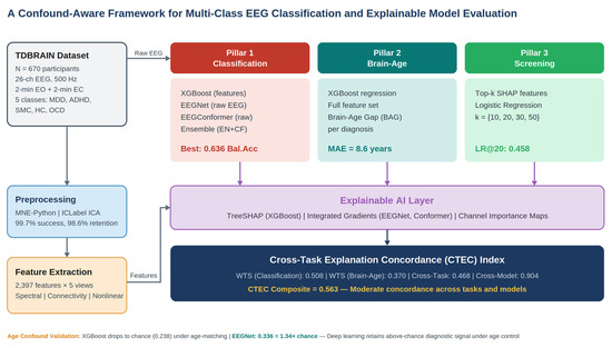
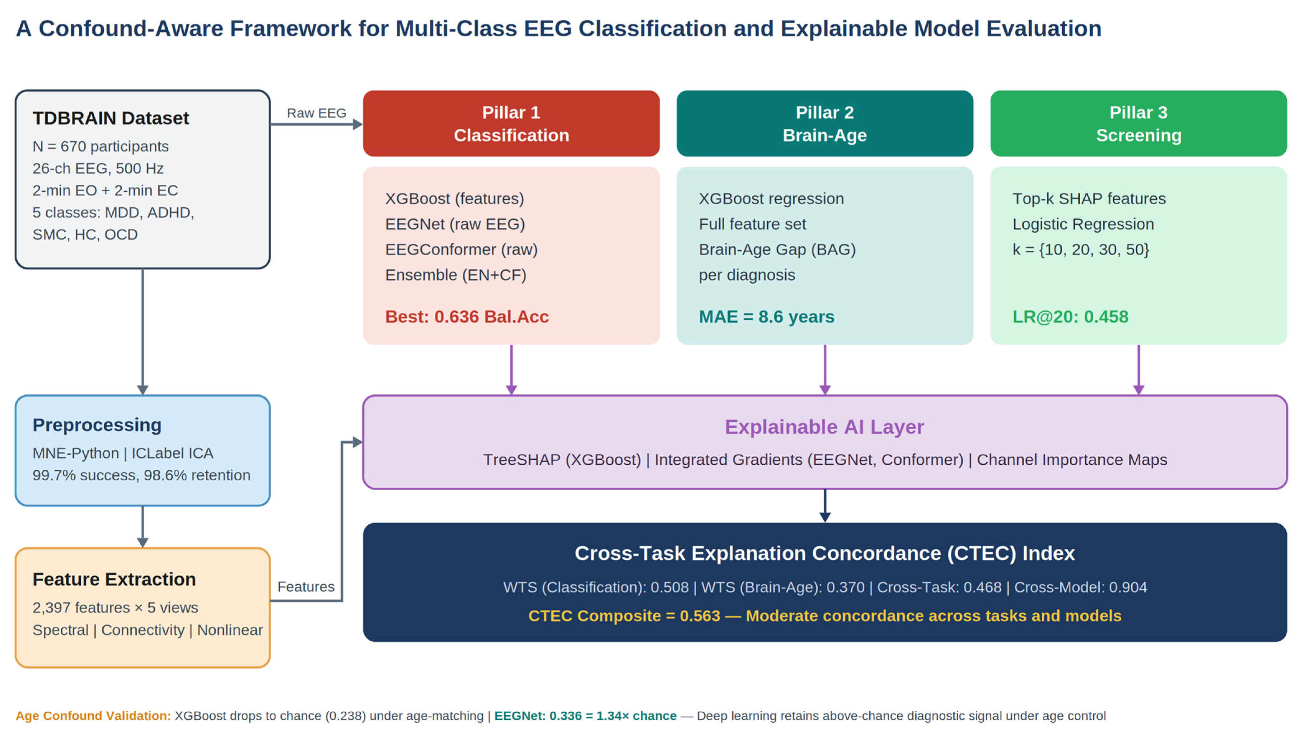
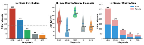
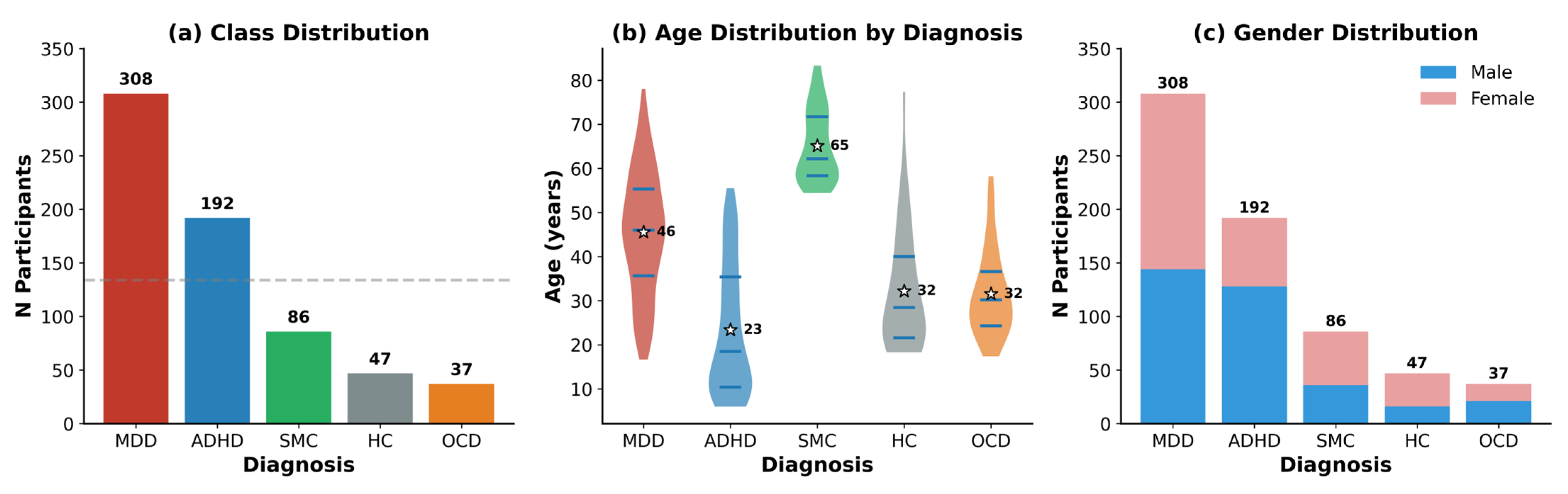
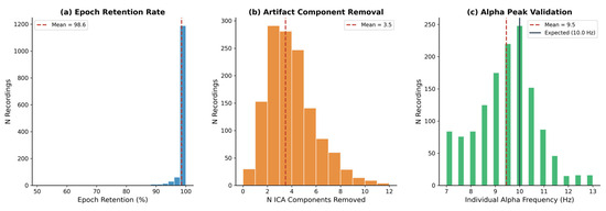
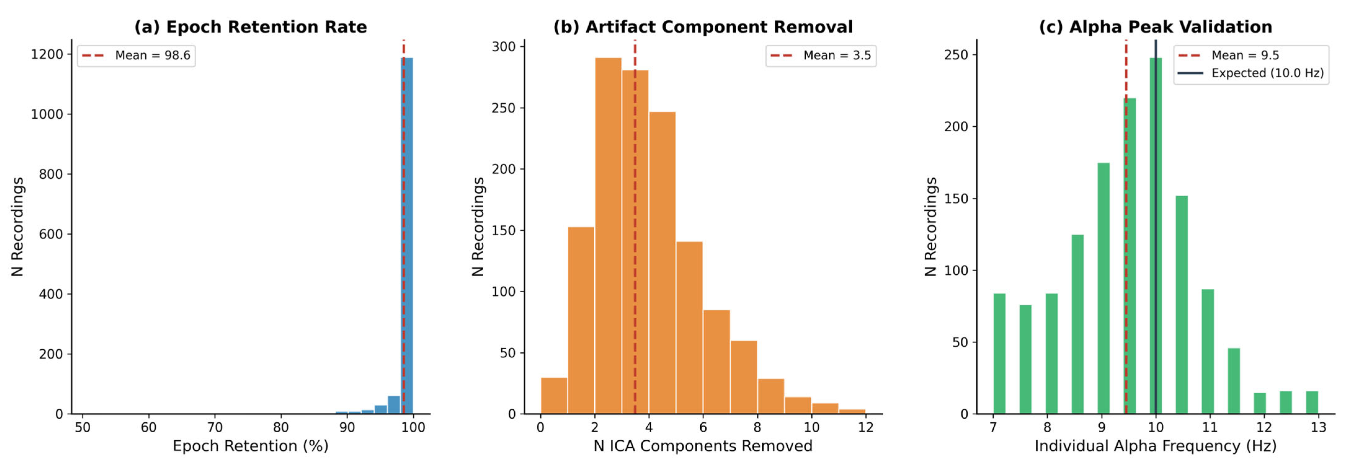
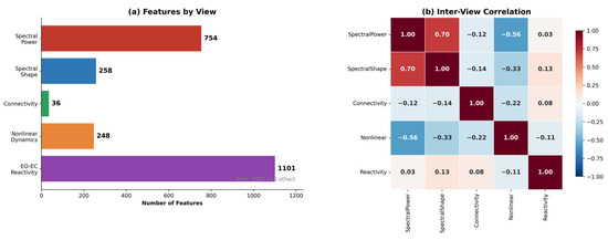
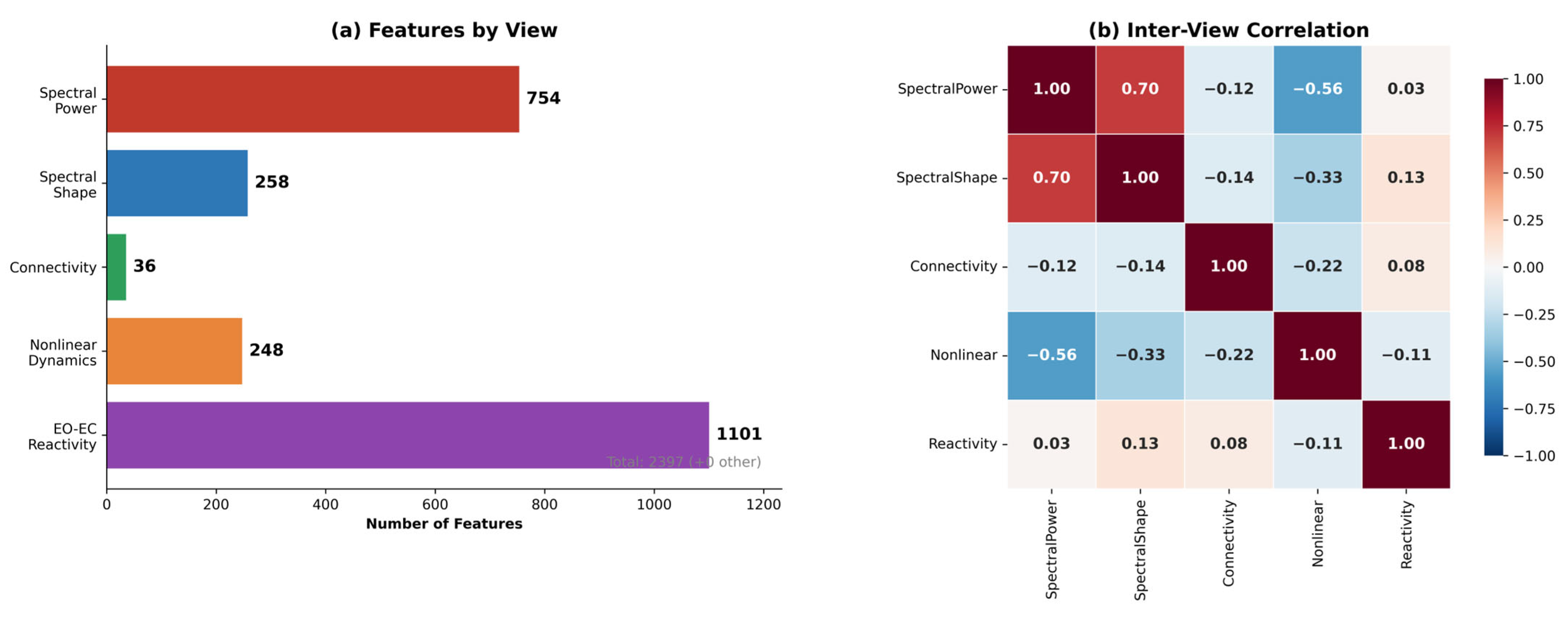

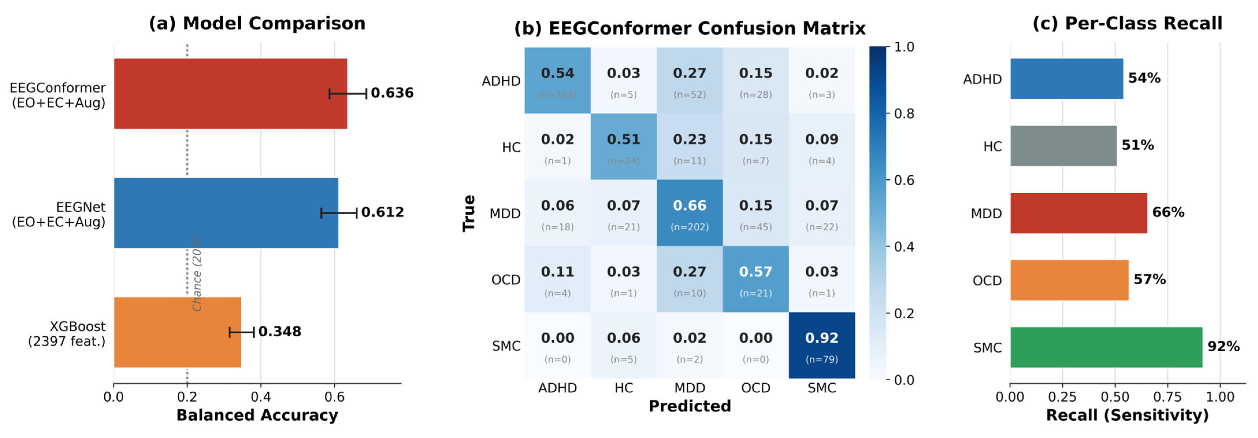
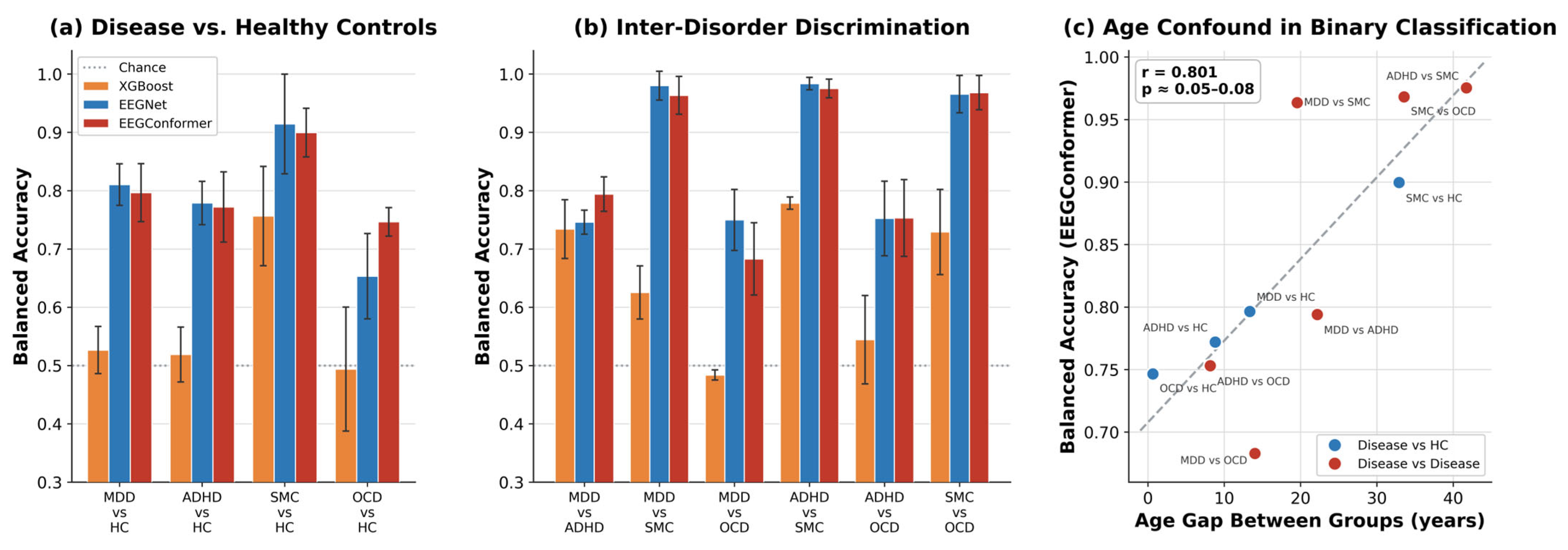
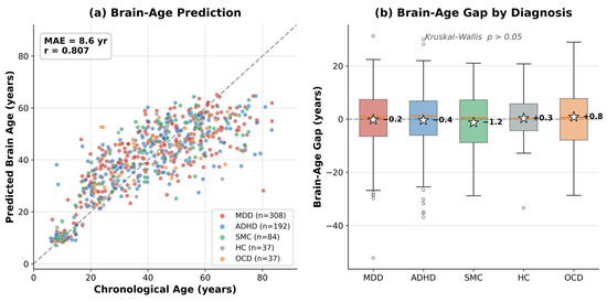
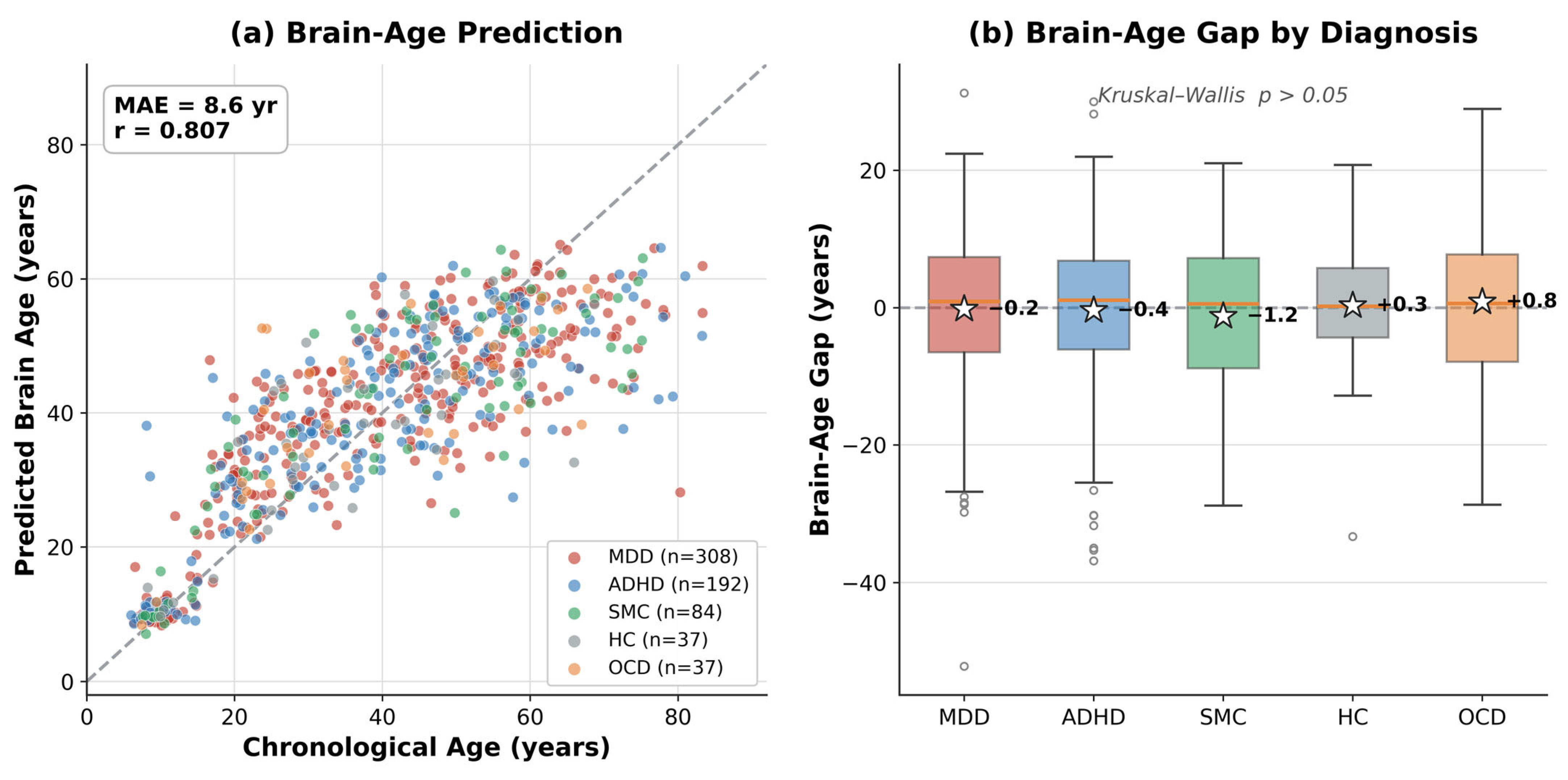
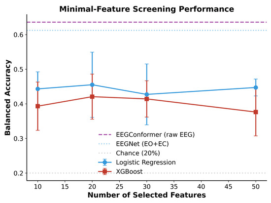
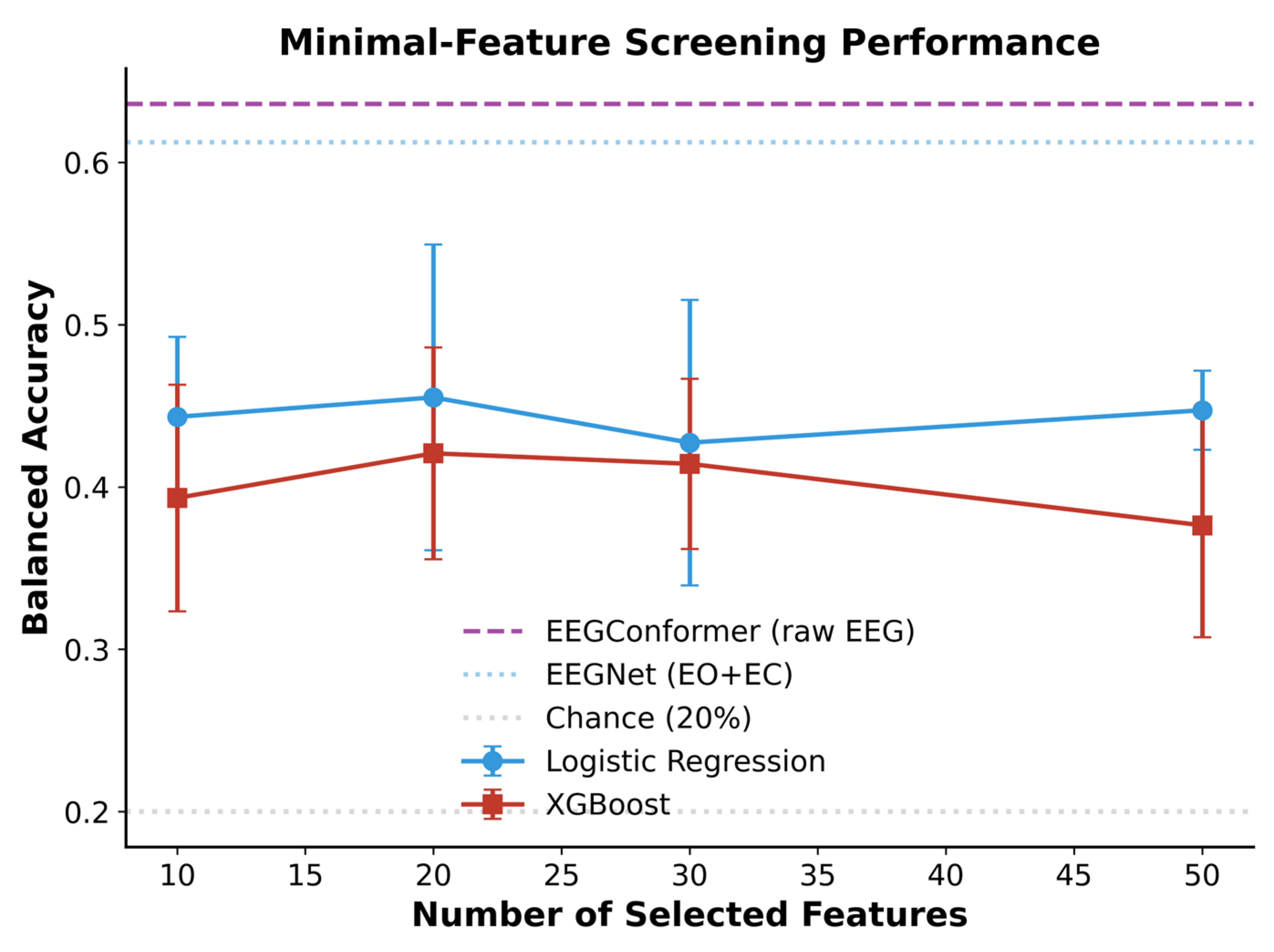
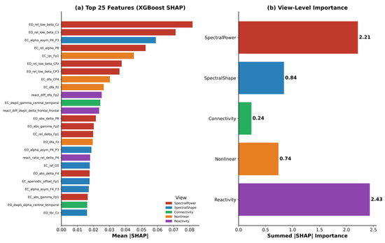
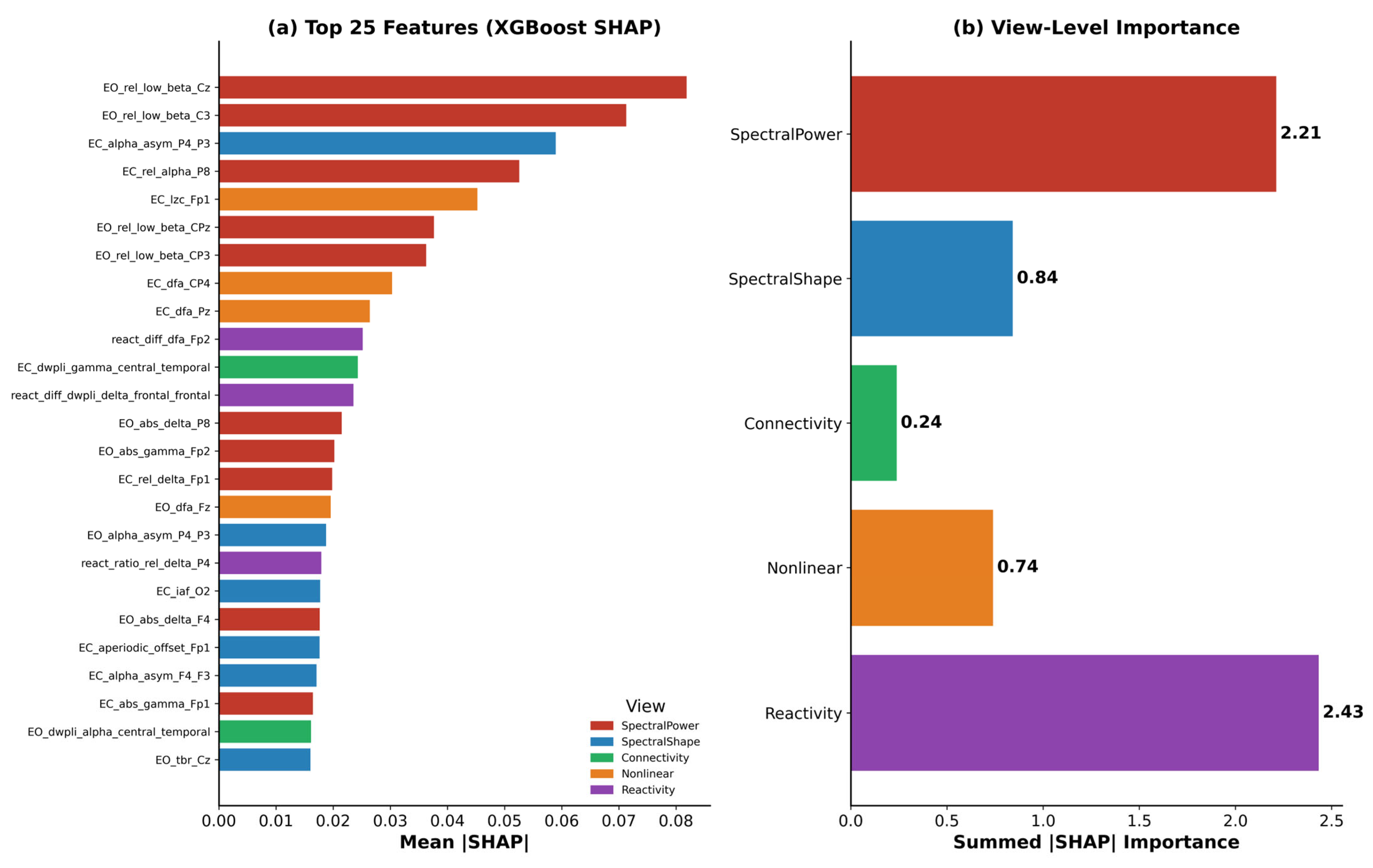
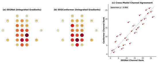
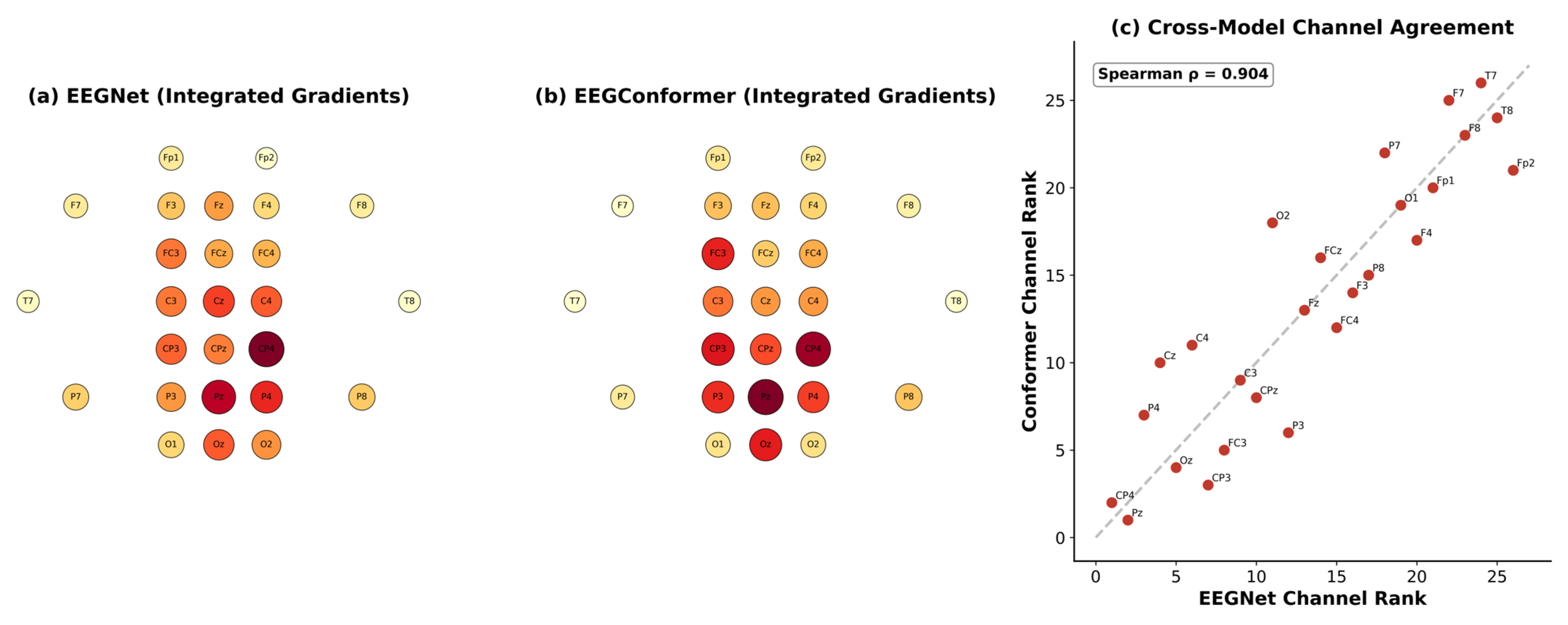
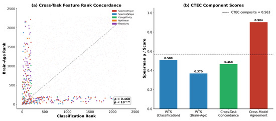
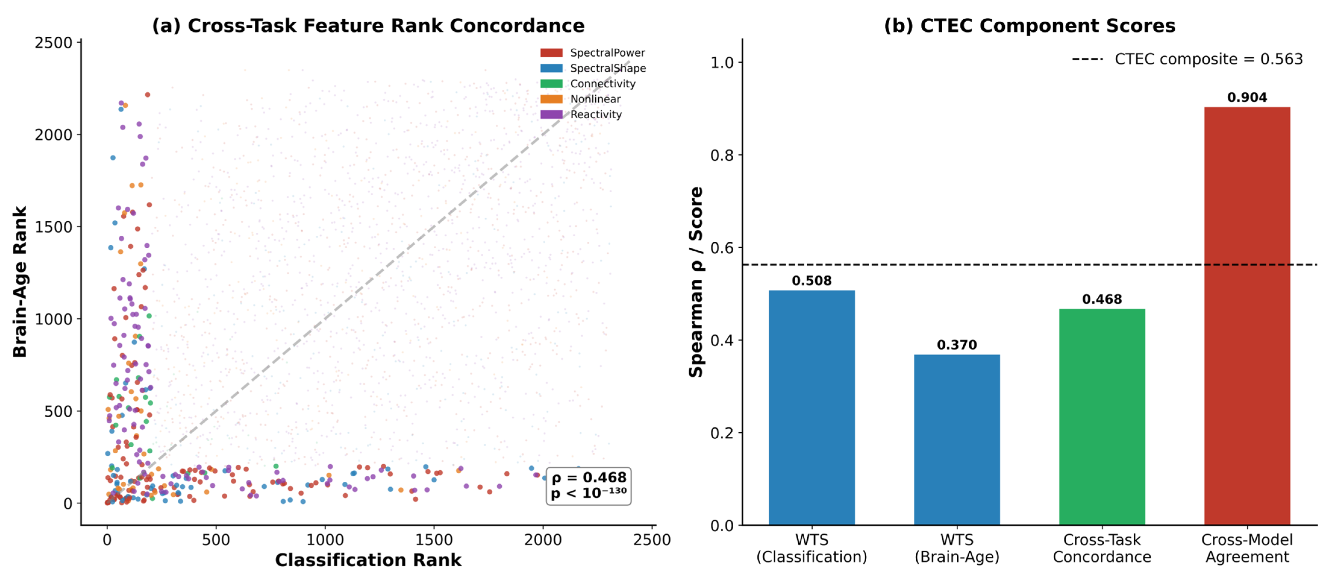
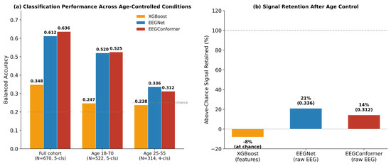
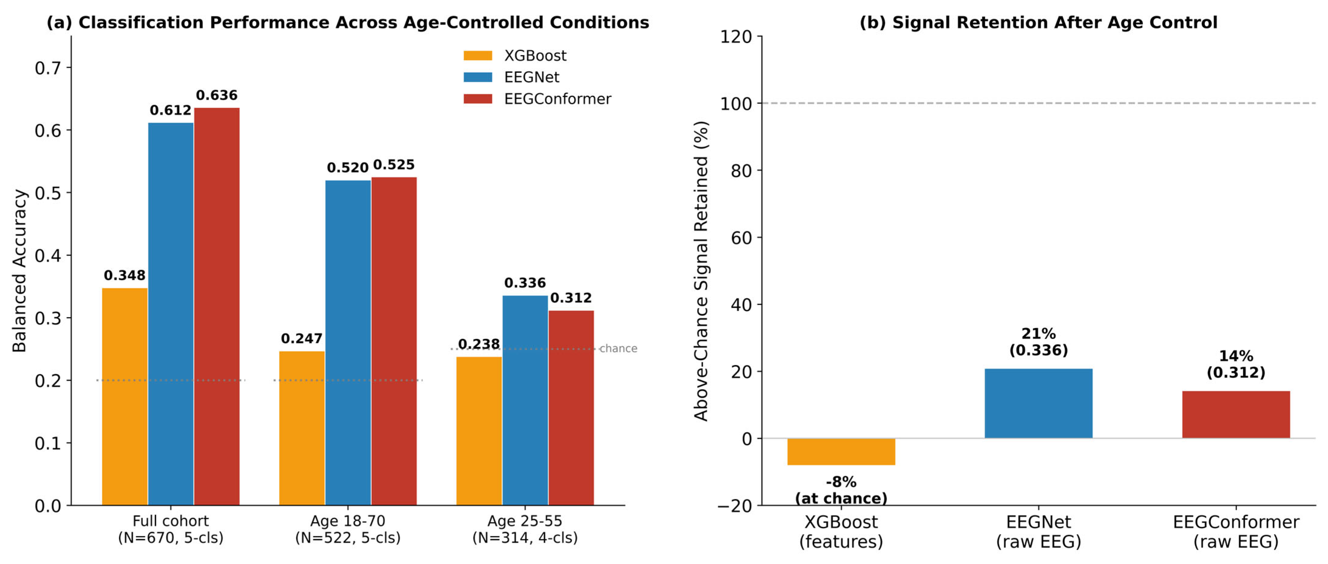
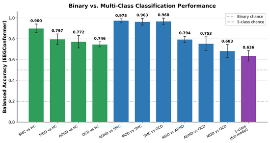
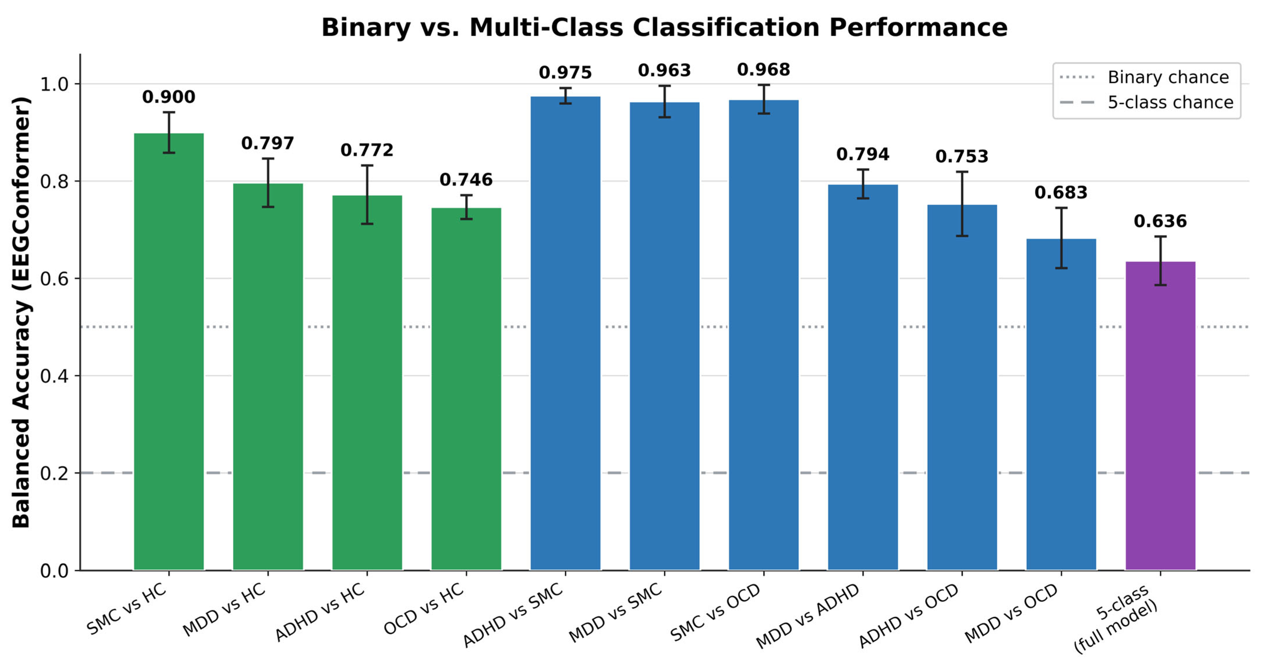

Disclaimer/Publisher’s Note: The statements, opinions and data contained in all publications are solely those of the individual author(s) and contributor(s) and not of MDPI and/or the editor(s). MDPI and/or the editor(s) disclaim responsibility for any injury to people or property resulting from any ideas, methods, instructions or products referred to in the content. |
© 2026 by the authors. Licensee MDPI, Basel, Switzerland. This article is an open access article distributed under the terms and conditions of the Creative Commons Attribution (CC BY) license.