Tricomi Problem for a Second-Kind Mixed-Type Equation in a Domain Whose Elliptic Part Is a Vertical Half-Strip

Abstract

In this paper, the Tricomi problem for a second-kind mixed-type equation with a lower-order term is studied in an unbounded domain. The elliptic part of the domain is a vertical half-strip, while the hyperbolic part is bounded by characteristics. Homogeneous Dirichlet conditions are imposed on the walls of the half-strip, gluing conditions are given on the parabolic degeneracy line, and the trace of the desired solution is prescribed on one of the characteristics. The uniqueness of the solution is proved using the extremum principle and the Zaremba–Giraud principle. The existence of the solution is established by Green’s function method: in the elliptic part, Green’s function of the mixed problem is constructed in the form of a rapidly convergent series; in the hyperbolic part, a generalized solution of the Cauchy problem of a special class is used. The functional relations on the degeneracy line lead to a singular integral equation, which is regularized by the Carleman–Vekua method into a Fredholm integral equation of the second kind with a weak singularity. Explicit formulas for the trace of the solution and its normal derivative are obtained. For a specific set of parameters, a numerical visualization of the solution is performed, the gluing conditions are verified, and a physical interpretation of the obtained graphs is given in the context of transonic gas dynamics. The results can be useful for mathematical modeling of flows in Laval nozzles and other problems of mechanics.

1. Introduction

A new stage in the development of the theory of boundary value problems for mixed-type equations is marked by the works of M.A. Lavrentiev [1], L. Bers [2], F.I. Frankl [3], and Chen Gui-Qiang G. [4], where the importance of the Tricomi problem and its generalizations is indicated in connection with transonic gas dynamics, magnetohydrodynamic flows with transition through the speed of sound and the Alfvén speed, the theory of infinitesimal bendings of surfaces, and many other issues of mechanics.

Most studies on mixed-type equations concern equations of the first kind with power degeneracy, for which the tangent to the parabolic line does not coincide with the characteristic direction. For the model equation of the first kind

$${\mathrm{sign}y\left|y\right|}^m{u}_{xx}+u_{yy}=0,m>0,$$

the Tricomi problem in a domain whose elliptic part is a vertical half-strip was studied for $m=1$ in [5] and for $m>0$ in [6]. In [7], this problem was investigated for the generalized Tricomi equation

$${\mathrm{sign}y\left|y\right|}^m{u}_{xx}+u_{yy}-{\lambda }^2{\left|y\right|}^{m}u=0,m>0,\lambda \in \mathbb{R}.$$

A physical justification of the Tricomi problem in domains where the elliptic part is a vertical half-strip was given in [8,9]. L.V. Ovsyannikov [8] used the velocity hodograph plane in the framework of transonic gas dynamics, where nonlinear equations become linear and near the speed of sound are approximated by the Tricomi equation. The approximate solution he constructed describes a transonic flow with a detached shock wave and a subsonic zone behind it in the form of a vertical half-strip; the sonic line corresponds to the parabolic degeneracy line $y=0$.

The Tricomi problem for the second-kind mixed-type equation

$$u_{xx}+\mathrm{sign}y{\left|y\right|}^m{u}_{yy}=0,0<m<1,$$

in a bounded domain was first considered by I.L. Karol [10]. The elliptic part was bounded by the normal curve $y={\left[{\displaystyle \frac{2-m}{4}}x(1-x)\right]}^{\frac{1}{2-m}}$, the hyperbolic part by characteristics, and the degeneracy line $y=0$ itself is a characteristic. Following the idea of F.D. Tricomi, the N problem (Holmgren) in the elliptic part and the Cauchy problem in the hyperbolic part were solved using Green’s function method, and then the solutions were glued together. The existence of the solution was reduced to an integral equation for $\nu \left(x\right)$, solvable due to the uniqueness theorem. Subsequent works (e.g., [11]) also considered bounded domains and used the representation of the N problem from [10]. It should be noted that the study of the N problem has not lost its relevance over time. For example, the article [12] examined the N problem for the Euler–Darboux equation with two degeneracy lines and its application to the problem of filtering contaminants in inhomogeneous media.

In the case where the elliptic part is a vertical half-strip, the shift problem on a characteristic of one family was studied in [13], where the N problem was solved by Green’s function method. A nonlocal problem for the generalized Tricomi equation with a spectral parameter in an unbounded domain, the elliptic part of which is the upper half-plane, is considered in the article [14]. If the elliptic part is a horizontal half-strip, a nonlocal problem of Bitsadze–Samarskii type was investigated in our recent work [15]. For a mixed-type equation of the first kind with a singular coefficient, a nonlocal problem in an unbounded domain was studied in [16]. For the Tricomi problem for a second-kind mixed-type equation in an unbounded domain whose elliptic part is the first quadrant of the plane, see [17].

To further motivate the present work, we recall several recent contributions that address related questions for mixed-type and degenerate elliptic equations with advanced analytical techniques. Zarubin and Chaplygina [18] investigated the Tricomi problem for a difference-differential equation of mixed type with a lumped delay in an unbounded domain. By combining the method of general solution with the Laplace integral transform, they proved unique solvability of the problem and obtained explicit functional relations on the type change line. Although their equation involves a delay term, the overall scheme—reducing the problem to integral and integro-difference equations—shares conceptual similarities with the approach used in the present work.

In the context of degenerate elliptic equations with singular coefficients, Ruziev and Kazakbaeva [19] studied a nonlocal boundary value problem in a vertical half-strip for the equation $y^m{u}_{xx}+u_{yy}+\frac{{\beta }_0}{y}{u}_y-{\lambda }^2{y}^{m}u=0$. Using the Hankel transform and the separation of variables, they constructed an explicit series solution, proved uniqueness via the maximum principle, and established existence under natural smoothness and decay conditions. Their work demonstrates how Green’s function method and series representations can be effectively applied in a vertical half-strip domain, which is precisely the shape of the elliptic part in our problem $T^{\infty }$.

The same authors [20] later considered a nonlocal boundary value problem for the Holmgren equation $y^m{u}_{xx}+u_{yy}+\frac{{\alpha }_0}{y^{1-m/2}}{u}_x+\frac{{\beta }_0}{y}{u}_y=0$ in the upper half-plane. Uniqueness was proved by the energy integral method, while existence was reduced either to a Fredholm integral equation of the second kind or to a singular integral equation with a Cauchy kernel, depending on the order of the Riemann–Liouville fractional derivative in the boundary condition. The singular equation was solved by the Carleman–Vekua method. These results are particularly relevant because our derivation of the functional relation from the hyperbolic part and the subsequent regularization of the singular integral equation follow a similar philosophy, albeit in a different geometry and with a different type of degeneracy.

Additionally, Mirsaburov and Turaev [21] studied a problem in an unbounded domain with combined Tricomi and Frankl conditions on one boundary characteristic for a class of mixed-type equations. They considered an equation of the first kind with a singular coefficient and, using the method of integral equations and the extremum principle, proved the unique solvability of the problem. Although their work deals with a different canonical form and a different type of boundary condition, their approach to constructing functional relations on the degeneracy line and to regularizing the resulting singular integral equations is methodologically close to the one employed in the present paper. The combination of Tricomi and Frankl conditions on a single characteristic provides additional insight into how mixed boundary conditions can be handled in unbounded domains.

The article is organized as follows. Section 2 recalls necessary facts from the theory of Riemann–Liouville fractional integro-differentiation and the main properties of the operators used. Section 3 states the problem $T^{\infty }$: the mixed domain, the class of generalized solutions ${\mathbb{R}}_2$ in the hyperbolic part, and the main functional relations on the degeneracy line. Section 4 is devoted to proving the uniqueness of the solution using the extremum principle and the Zaremba–Giraud principle. Section 5 presents the proof of existence: Green’s function method constructs a representation of the solution in the elliptic half-strip, a singular integral equation for the normal derivative is derived, its Carleman–Vekua regularization reduces it to a Fredholm integral equation of the second kind; then, explicit formulas for $\tau \left(x\right)$ and $\nu \left(x\right)$ are given. Section 6 contains a concrete example with $m=1$, $\alpha =0.25$ and $\psi \left(x\right)=x^{6/5}{(1/2-x)}^{6/5}$, as well as a visualization of the solution, consistency checks, and physical interpretation. Section 7 formulates the main conclusions of the work.

2. Preliminaries

In this section, we recall the definitions of Riemann–Liouville fractional integrals and derivatives, as well as their main properties that will be used in the paper (for more details, see [22,23,24]).

Let the function $f\left(x\right)$ be defined on the interval $[0,1]$ and let $\mu >0$. The left-sided and right-sided fractional integrals of order $\mu$ are defined respectively by

$$I_{0+}^{\mu }f\left(x\right)=\frac{1}{\mathsf{\Gamma }\left(\mu \right)}{\int }_0^x{(x-t)}^{\mu -1}f\left(t\right)dt,I_{1-}^{\mu }f\left(x\right)=\frac{1}{\mathsf{\Gamma }\left(\mu \right)}{\int }_x^1{(t-x)}^{\mu -1}f\left(t\right)dt.$$

The Riemann–Liouville fractional derivatives of order $\mu >0$ are introduced by integer-order differentiation of the fractional integral. If $n=\left[\mu \right]+1$, then

$$D_{0+}^{\mu }f\left(x\right)={\displaystyle \frac{d^n}{d{x}^n}}{I}_{0+}^{n-\mu }f\left(x\right),D_{1-}^{\mu }f\left(x\right)={(-1)}^n{\displaystyle \frac{d^n}{d{x}^n}}{I}_{1-}^{n-\mu }f\left(x\right).$$

For $\mu =0$, we set $I_{0+}^{0}f=f$, $D_{0+}^{0}f=f$. For negative order, the fractional derivative coincides with the integral $D_{0+}^{-\mu }=I_{0+}^{\mu }$ ($\mu >0$), and similarly for the right endpoint.

We now introduce the modified operators $D_{0x}^a$ and $D_{x1}^a$ (see Formulas (1) and (2) below), which are directly used in the problem statement and in the subsequent derivations. They retain the main properties of fractional integro-differentiation listed in items (i)–(iv).

$$D_{0x}^{a}f\left(x\right)=\left\{\begin{array}{cc}{\displaystyle \frac{1}{\mathsf{\Gamma }(-a)}{\int }_0^x{(x-t)}^{-(a+1)}f\left(t\right)dt,}\hfill & a<0,\hfill \\ {\displaystyle \frac{d^{n+1}}{d{x}^{n+1}}{D}_{0x}^{a-(n+1)}f\left(x\right),}\hfill & a>0,\hfill \end{array}\right.$$

(1)

$$D_{x1}^{a}f\left(x\right)=\left\{\begin{array}{cc}{\displaystyle \frac{1}{\mathsf{\Gamma }(-a)}{\int }_x^1{(t-x)}^{-(a+1)}f\left(t\right)dt,}\hfill & a<0,\hfill \\ {\displaystyle -\frac{d^{n+1}}{d{x}^{n+1}}{D}_{x1}^{a-(n+1)}f\left(x\right),}\hfill & a>0,\hfill \end{array}\right.$$

(2)

where a is any real number and n is the integer part of a when $a\ge n$.

Properties of the operators ${\mathit{D}}_{\mathbf{0}\mathit{x}}^{\mathit{a}}$ and ${\mathit{D}}_{\mathit{x}\mathbf{1}}^{\mathit{a}}$. For sufficiently smooth functions (with the regularity conditions indicated below), the following relations hold.

(i)

Semigroup property. For any $p>0$, $q>0$ and a function f,

$$D_{0x}^{-p}{D}_{0x}^{-q}f=D_{0x}^{-(p+q)}f,D_{x1}^{-p}{D}_{x1}^{-q}f=D_{x1}^{-(p+q)}f,$$

where a negative order means the fractional integral (see (1), (2) for $a<0$).

(ii)

Relation with the derivative. If $r>0$, then $D_{0x}^r{D}_{0x}^{-r}f=f$. If f is such that the fractional derivative $D_{0x}^{r}f$ exists and is summable, and, in addition, $D_{0x}^{r-n}f\in A{C}^n$ (i.e., $D_{0x}^{r-n}f$ and its derivatives up to order $n-1$ are absolutely continuous), where $n=\lceil r\rceil$ (the smallest integer greater than or equal to r), then the following analog of Taylor’s formula holds:

$$D_{0x}^{-r}{D}_{0x}^{r}f\left(x\right)=f\left(x\right)-{\displaystyle \sum _{k=1}^n}{c}_k{x}^{r-k},$$

with constants $c_k$. For integer r, this reduces to the classical Taylor expansion. Similar formulas hold for the right operator $D_{x1}^r$.

(iii)

Action on power functions. For $q>0$ and real p such that $q-p\notin \{0,-1,-2,\dots \}$,

$$D_{0x}^p{x}^{q-1}={\displaystyle \frac{\mathsf{\Gamma }\left(q\right)}{\mathsf{\Gamma }(q-p)}}{x}^{q-p-1},D_{x1}^p{(1-x)}^{q-1}={\displaystyle \frac{\mathsf{\Gamma }\left(q\right)}{\mathsf{\Gamma }(q-p)}}{(1-x)}^{q-p-1}.$$

(iv)

Composition of oppositely directed operators. For any $p,q$ with $0<p<q$,

$$D_{0x}^{p-q}\left[x^{q-1}\right]={\displaystyle \frac{\mathsf{\Gamma }\left(q\right)}{\mathsf{\Gamma }(q-p)}}{x}^{q-p-1}.$$

This property is used in the regularization of the singular integral equation. An analogous relation holds for $D_{x1}^{p-q}$ with x replaced by $1-x$.

All the properties (i)–(iv) for the operators $D_{0x}^a$ and $D_{x1}^a$ follow from the corresponding properties of the classical Riemann–Liouville operators, taking into account the sign conventions in definitions (1) and (2). Only these modified operators are used in the remainder of the paper.

3. Problem Statement

Consider the equation

$$u_{xx}+{\mathrm{sign}y\left|y\right|}^m{u}_{yy}+\alpha {\left|y\right|}^{m-1}{u}_y=0,1\le m<2,m-1<\alpha <1,$$

(3)

in the unbounded mixed domain $\mathsf{\Omega }={\mathsf{\Omega }}_1\cup l_0\cup {\mathsf{\Omega }}_2$, where

$${\mathsf{\Omega }}_1=\{(x,y):0<x<1,0<y<+\infty \},l_0=\{(x,y):0<x<1,y=0\},$$

and ${\mathsf{\Omega }}_2$ is the domain in the half-plane $y<0$ bounded by the segment $AB$ of the $Ox$ axis and by the two characteristics

$$AC:x-{\displaystyle \frac{2}{2-m}}{(-y)}^{(2-m)/2}=0,BC:x+{\displaystyle \frac{2}{2-m}}{(-y)}^{(2-m)/2}=1$$

of Equation (3) emanating from the point $C\left({\displaystyle \frac{1}{2}},-{\left({\displaystyle \frac{2-m}{4}}\right)}^{\frac{2}{2-m}}\right)$. We introduce the notation

$$l_1=\{(x,y):x=0,0\le y<+\infty \},l_2=\{(x,y):x=1,0\le y<+\infty \}.$$

In the half-plane $y<0$, Equation (3) takes the form

$$u_{xx}-{(-y)}^m{u}_{yy}+\alpha {(-y)}^{m-1}{u}_y=0.$$

(4)

In the characteristic coordinates

$$\xi =x-{\displaystyle \frac{2}{2-m}}{(-y)}^{(2-m)/2},\eta =x+{\displaystyle \frac{2}{2-m}}{(-y)}^{(2-m)/2},$$

(5)

Equation (4) transforms into the Euler–Darboux equation

$${\displaystyle \frac{{\partial }^{2}u}{\partial \xi \partial \eta }}-{\displaystyle \frac{\beta }{\eta -\xi }}\left({\displaystyle \frac{\partial u}{\partial \eta }}-{\displaystyle \frac{\partial u}{\partial \xi }}\right)=0,$$

(6)

with

$$\beta ={\displaystyle \frac{2\alpha -m}{2(2-m)}},-{\displaystyle \frac{1}{2}}<\beta <0,m-1<\alpha <{\displaystyle \frac{m}{2}}.$$

(7)

It is known that the solution of the Cauchy problem for Equation (6) with initial conditions

$$\underset{y\to 0}{\lim }u(x,y)=\tau \left(x\right),0\le x\le 1,$$

$$\underset{y\to -0}{\lim }{(-y)}^{\alpha }{u}_y(x,y)={\left[{\displaystyle \frac{2-m}{4}}\right]}^{2\beta }\underset{\eta -\xi \to 0}{\lim }{(\eta -\xi )}^{2\beta }(u_{\xi }-u_{\eta })=\nu \left(x\right),0<x<1,$$

(8)

has the form (see [5])

$$\begin{array}{cc}\hfill u(\xi ,\eta )& =k_1{\int }_0^1\tau \left(\xi +(\eta -\xi )t\right)t^{\beta }{(1-t)}^{\beta }dt\hfill \\ \hfill & +{\displaystyle \frac{k_1(\eta -\xi )}{2(1+2\beta )}}{\int }_0^1{\tau }^{\prime }\left(\xi +(\eta -\xi )t\right)t^{\beta }{(1-t)}^{\beta }(2t-1)dt\hfill \\ \hfill & -k_2{(\eta -\xi )}^{1-2\beta }{\int }_0^1\nu \left(\xi +(\eta -\xi )t\right)t^{-\beta }{(1-t)}^{-\beta }dt,\hfill \end{array}$$

(9)

where

$$k_1={\displaystyle \frac{\mathsf{\Gamma }(2+2\beta )}{{\mathsf{\Gamma }}^2(1+\beta )}},k_2={\left[{\displaystyle \frac{2-m}{4}}\right]}^{1-2\beta }{\displaystyle \frac{\mathsf{\Gamma }(2-2\beta )}{(1-\alpha ){\mathsf{\Gamma }}^2(1-\beta )}}.$$

Returning to the original variables x and y, we obtain

$$u(x,y)=k_1{\int }_0^1\tau \left(x+{\displaystyle \frac{2}{2-m}}{(-y)}^{{\displaystyle \frac{2-m}{2}}}(2t-1)\right)t^{\beta }{(1-t)}^{\beta }dt+$$

$$+{\displaystyle \frac{2k_1}{(1+2\beta )(2-m)}}{(-y)}^{{\displaystyle \frac{2-m}{2}}}{\int }_0^1{\tau }^{\prime }\left(x+{\displaystyle \frac{2}{2-m}}{(-y)}^{{\displaystyle \frac{2-m}{2}}}(2t-1)\right)t^{\beta }{(1-t)}^{\beta }(2t-1)dt-$$

(10)

$$-{\left[{\displaystyle \frac{2-m}{4}}\right]}^{2\beta -1}{k}_2{(-y)}^{1-\alpha }{\int }_0^1\nu \left(x+{\displaystyle \frac{2}{2-m}}{(-y)}^{{\displaystyle \frac{2-m}{2}}}(2t-1)\right)t^{-\beta }{(1-t)}^{-\beta }dt.$$

For any $\tau \left(x\right)\in C^3[0,1]$ and $\nu \left(x\right)\in C^2[0,1]$, the expression (10) is a twice continuously differentiable solution of the Cauchy problem for Equation (4) with initial data (8) in the domain ${\mathsf{\Omega }}_2$.

An expression of the form (9) or (10) will be called a generalized solution of Equation (4) in ${\mathsf{\Omega }}_2$ if $\tau \left(x\right)$ and $\nu \left(x\right)$ are continuous for $0<x<1$.

In ${\mathsf{\Omega }}_2$, we consider the following class ${\mathbb{R}}_2$ of generalized solutions of the Cauchy problem introduced in [5].

Definition 1. 

A generalized solution (9) or (10) of Equation (4) belongs to the class ${\mathbb{R}}_2$ if $\nu \left(x\right)$ is continuous and integrable for $0<x<1$, and $\tau \left(x\right)$ is a fractional integral of order $-(2\beta -1)$ of some function $T\left(x\right)$ continuous and integrable on $(0,1)$, i.e.,

$$\tau \left(x\right)=\tau \left(0\right)+{\int }_0^{x}T\left(t\right){(x-t)}^{-2\beta }dt.$$

(11)

Without loss of generality, we assume $\tau \left(0\right)=0$; from (11) it follows that $\tau \left(x\right)\in [0,1]$ and ${\tau }^{\prime }\left(x\right)$ exists on $(0,1)$. The following lemmas hold [5].

Lemma 1. 

A generalized solution $u(x,y)\in {\mathbb{R}}_2$ is continuous in the closed domain $\overline{{\mathsf{\Omega }}_2}$.

Lemma 2. 

If a generalized solution $u(x,y)\in {\mathbb{R}}_2$, then the derivatives $u_x$ and $u_y$ are continuous in ${\mathsf{\Omega }}_2$ and

$$\underset{y\to -0}{\lim }{(-y)}^{\alpha }{u}_y(x,y)=\nu \left(x\right),0<x<1.$$

Making the substitution $\zeta =\xi +(\eta -\xi )t$ in Formula (9), we represent $u(\xi ,\eta )$ in the form

$$u(\xi ,\eta )=k_1{(\eta -\xi )}^{-1-2\beta }{\displaystyle \underset{\xi }{\overset{\eta }{\int }}}\tau \left(\zeta \right){(\eta -\zeta )}^{\beta }{(\zeta -\xi )}^{\beta }d\zeta -$$

$$-{\displaystyle \frac{k_1{(\eta -\xi )}^{-1-2\beta }}{2(1+\beta )}}{\displaystyle \underset{\xi }{\overset{\eta }{\int }}}{\tau }^{\prime }\left(\zeta \right)\left[{(\eta -\zeta )}^{1+\beta }{(\zeta -\xi )}^{\beta }-{(\eta -\zeta )}^{\beta }{(\zeta -\xi )}^{1+\beta }\right]d\zeta -$$

(12)

$$-k_2{\displaystyle \underset{\xi }{\overset{\eta }{\int }}}\nu \left(\zeta \right){(\eta -\zeta )}^{-\beta }{(\zeta -\xi )}^{-\beta }d\zeta .$$

Now, substituting (11) into Formula (12), after some transformations we obtain

$$u(\xi ,\eta )={\displaystyle \underset{0}{\overset{\xi }{\int }}}T\left(t\right){(\eta -t)}^{-\beta }{(\xi -t)}^{-\beta }dt+$$

(13)

$$+{\displaystyle \frac{1}{2\cos \pi \beta }}{\displaystyle \underset{\xi }{\overset{\eta }{\int }}}T\left(t\right){(\eta -t)}^{-\beta }{(t-\xi )}^{-\beta }dt-k_2{\displaystyle \underset{\xi }{\overset{\eta }{\int }}}\nu \left(t\right){(\eta -t)}^{-\beta }{(t-\xi )}^{-\beta }dt$$

From (13), the main functional relation between $\tau \left(x\right)$ and $\nu \left(x\right)$ obtained from the hyperbolic region ${\mathsf{\Omega }}_2$ of Equation (3) is obtained in the following form [5]:

$$\tau \left(x\right)=k_3{\int }_0^x\nu \left(t\right){(x-t)}^{-2\beta }dt+F_1\left(x\right),0\le x\le 1,$$

(14)

where

$$F_1\left(x\right)={\displaystyle \frac{\mathsf{\Gamma }\left(\beta \right)}{\mathsf{\Gamma }\left(2\beta \right)}}{D}_{0x}^{2\beta -1}\left[x^{\beta }{D}_{0x}^{1-\beta }\psi \left(x\right)\right],k_3=2\cos \pi \beta k_2,$$

and $\psi \left(x\right)$ is a given function with $\psi \left(0\right)=0$, $\psi \left(x\right)\in C^1[0,1]\cap C^2(0,1)$.

Problem 1 

(Problem $T^{\infty }$). Find a function $u(x,y)$ with the following properties:

 (1) 

$u(x,y)\in C\left(\overline{\mathsf{\Omega }}\right)$ where $\overline{\mathsf{\Omega }}=\overline{{\mathsf{\Omega }}_2}\cup {\mathsf{\Omega }}_1\cup \overline{l_1}\cup \overline{l_2}$;

 (2) 

$u(x,y)\in C^2\left({\mathsf{\Omega }}_1\right)$ and satisfies Equation (3) in ${\mathsf{\Omega }}_1$;

 (3) 

$u(x,y)$ is a generalized solution of class ${\mathbb{R}}_2$ in ${\mathsf{\Omega }}_2$;

 (4) 

The partial derivative $u_y(x,y)$ satisfies the gluing condition

$$\underset{y\to +0}{\lim }{(-y)}^{\alpha }{u}_y(x,y)=-\underset{y\to -0}{\lim }{y}^{\alpha }{u}_y(x,y)=\nu \left(x\right),0<x<1,$$

which arises in solving the direct problem of Laval nozzle theory, and $u_y(x,0)$ may have a singularity of order less than one at the ends of the interval $(0,1)$;

 (5) 

$u(x,y)$ satisfies the boundary conditions

$$u(0,y)=0,u(1,y)=0,0\le y<+\infty ,$$

(15)

$$\underset{y\to +\infty }{\lim }u(x,y)=0uniformlyinx\in [0,1],$$

(16)

$$u(x,y){|}_{AC}=\psi \left(x\right),0\le x\le {\displaystyle \frac{1}{2}}.$$

(17)

4. Uniqueness of the Solution

Theorem 1. 

Problem $T^{\infty }$ has at most one solution.

Proof. 

Let $u(x,y)$ be a solution of the homogeneous problem $T^{\infty }$ ($\psi \left(x\right)\equiv 0$). Then relation (14) becomes

$$\tau \left(x\right)=k_3{\int }_0^x\nu \left(t\right){(x-t)}^{-2\beta }dt.$$

(18)

According to the definition of the operator $D_{0x}^a$ for $a<0$ (2), for $a=2\beta -1$ we have

$$D_{0x}^{2\beta -1}\nu \left(x\right)={\displaystyle \frac{1}{\mathsf{\Gamma }(1-2\beta )}}{\int }_0^x\nu \left(t\right){(x-t)}^{-2\beta }dt.$$

Consequently, (18) can be written as

$$\tau \left(x\right)=k_3\mathsf{\Gamma }(1-2\beta )D_{0x}^{2\beta -1}\nu \left(x\right).$$

Apply the operator $D_{0x}^{1-2\beta }$ (of order $1-2\beta \in (1,2)$) to both sides. By the semigroup property (ii), $D_{0x}^{1-2\beta }{D}_{0x}^{2\beta -1}\nu =\nu$, whence

$$D_{0x}^{1-2\beta }\tau \left(x\right)=k_3\mathsf{\Gamma }(1-2\beta )\nu \left(x\right).$$

(19)

For the fractional derivative of order $\alpha =1-2\beta \in (1,2)$ under the condition $\tau \left(0\right)=0$, the well-known Marchaud-type representation holds [22]:

$$D_{0x}^{1-2\beta }\tau \left(x\right)={\displaystyle \frac{\mathsf{\Gamma }(1-2\beta )\sin \pi \beta }{\pi }}\left[x^{2\beta -1}\tau \left(x\right)+(1-2\beta ){\int }_0^x{\displaystyle \frac{\tau \left(x\right)-\tau \left(t\right)}{{(x-t)}^{2-2\beta }}}dt\right].$$

Substituting this expression into (19) and canceling the common factor $\mathsf{\Gamma }(1-2\beta )$, we directly obtain

$$\nu \left(x\right)={\displaystyle \frac{\sin \pi \beta }{\pi }}\left[x^{2\beta -1}\tau \left(x\right)+(1-2\beta ){\int }_0^x{\displaystyle \frac{\tau \left(x\right)-\tau \left(t\right)}{{(x-t)}^{2-2\beta }}}dt\right].$$

(20)

First, we prove that $u(x,y)\equiv 0$ in $\mathsf{\Omega }\cup \overline{l_1}\cup \overline{l_2}\cup \overline{AB}$. Assume the contrary. Then there exists a domain ${\mathsf{\Omega }}_{1\rho }=\{(x,y):0<x<1,0<y<\rho \}$ in which $u(x,y)\not\equiv 0$. Consequently,

$$\underset{{\overline{\mathsf{\Omega }}}_{1\rho }}{\sup }\left|u(x,y)\right|>0$$

and this value is attained at some point $(x_0,y_0)\in {\overline{\mathsf{\Omega }}}_{1\rho }$.

Denote $\partial {\mathsf{\Omega }}_{1\rho }=AB\cup BD\cup DP\cup PA$, where

$$AB=\left\{\right(x,y):0<x<1,y=0\},BD=\left\{\right(x,y):x=1,0<y<\rho \},$$

$$DP=\left\{\right(x,y):0<x<1,y=\rho \},PA=\left\{\right(x,y):x=0,0<y<\rho \}.$$

By the extremum principle for elliptic equations [25], we have $(x_0,y_0)\notin {\mathsf{\Omega }}_{1\rho }$. In view of condition (15), $(x_0,y_0)\notin \overline{BD}\cup \overline{PA}$. Hence $(x_0,y_0)\in AB\cup \overline{DP}$.

Suppose $(x_0,y_0)\in AB$, i.e.,

$$\underset{{\overline{\mathsf{\Omega }}}_{1\rho }}{\sup }\left|u(x,y)\right|=\underset{\overline{AB}}{\sup }\left|u(x,y)\right|=|u(x_0,0)|>0,0<x_0<1.$$

If $u(x_0,0)>0$ (respectively $<0$), i.e., $(x_0,0)$ is a point of positive maximum (negative minimum) of $u(x,y)$, then from (20) it follows that $\nu \left(x_0\right)>0$ ($<0$). On the other hand, by the Zaremba–Giraud principle [25], $\nu \left(x_0\right)<0$ ($>0$). This contradiction shows that $(x_0,y_0)\notin AB$. Therefore, $(x_0,y_0)\in \overline{DP}$, i.e.,

$$\underset{{\overline{\mathsf{\Omega }}}_{1\rho }}{\sup }\left|u(x,y)\right|=\underset{0\le x\le 1}{\sup }\left|u(x,\rho )\right|>0.$$

Take an arbitrary number ${\rho }_1>\rho$. By the same argument, we obtain

$$\underset{{\overline{\mathsf{\Omega }}}_{1{\rho }_1}}{\sup }\left|u(x,y)\right|=\underset{0\le x\le 1}{\sup }\left|u(x,{\rho }_1)\right|>0.$$

Since ${\mathsf{\Omega }}_{1\rho }\subset {\mathsf{\Omega }}_{1{\rho }_1}$, we have

$$\underset{0\le x\le 1}{\sup }|u(x,{\rho }_1)|\ge \underset{0\le x\le 1}{\sup }\left|u(x,\rho )\right|>0,$$

which implies ${\lim }_{y\to +\infty }u(x,y)\not\equiv 0$, contradicting condition (16).

Hence $u(x,y)\equiv 0$ for $(x,y)\in {\mathsf{\Omega }}_1\cup l_1\cup l_2\cup \overline{AB}$. Since $u(x,0)=\tau \left(x\right)\equiv 0$, it follows from (18) that $\nu \left(x\right)\equiv 0$. Then, by formula (12), $u(x,y)\equiv 0$ in $\overline{{\mathsf{\Omega }}_2}$. Consequently, $u(x,y)\equiv 0$ in $\mathsf{\Omega }\cup l_1\cup l_2\cup \overline{AC}\cup \overline{BC}$, which proves the theorem. □

5. Existence of the Solution

We now proceed to prove the existence of a solution of problem $T^{\infty }$. In the half-plane $y>0$, Equation (3) takes the form

$$u_{xx}+y^m{u}_{yy}+\alpha y^{m-1}{u}_y=0.$$

(21)

Solving the $N^{\infty }$ problem by Green’s function method in the domain ${\mathsf{\Omega }}_1$, we obtain

$$u(x,y)=-{\int }_0^1\nu \left(t\right){\left[z^{m-\alpha }G(t,z;x,y)\right]}_{z=0}dt,$$

(22)

where $G(t,z;x,y)$ is Green’s function of the $N^{\infty }$ problem, given by

$$G(t,z;x,y)={\displaystyle \sum _{n=-\infty }^{+\infty }}\left[q_1(t+2n,z;x,y)-q_1(-t+2n,z;x,y)\right],$$

with

$$q_1(t,z;x,y)=k_4{z}^{\alpha -m}{r}_1^{-2\beta }F\left(\beta ,\beta ,2\beta ;{\displaystyle \frac{16{\left(zy\right)}^{(2-m)/2}}{{(2-m)}^2{r}_1^2}}\right)$$

being a fundamental solution of Equation (21). Here $F(a,b,c;z)$ is the Gauss hypergeometric function [26],

$$k_4={\displaystyle \frac{1}{4\pi }}{\left({\displaystyle \frac{4}{2-m}}\right)}^{2\beta }{\displaystyle \frac{{\mathsf{\Gamma }}^2\left(\beta \right)}{\mathsf{\Gamma }\left(2\beta \right)}},r_1^2={(t-x)}^2+{\displaystyle \frac{4}{{(2-m)}^2}}{\left(z^{(2-m)/2}+y^{(2-m)/2}\right)}^2.$$

Green’s function of the $N^{\infty }$ problem for Equation (3) is constructed by the reflection method [27,28], using the mean value theorem and estimates for the hypergeometric function

$$F(a,b,c;x)=\left\{\begin{array}{cc}{M}_1,\hfill & c-a-b>0,0\le x\le 1,\hfill \\ M_1{(1-x)}^{c-a-b},\hfill & c-a-b<0,0<x<1,\hfill \\ M_1[1+\ln (1-x)],\hfill & c-a-b=0,0<x<1,\hfill \end{array}\right.$$

where $M_1>0$ is a constant.

One can prove explicit estimates for Green’s function and its derivatives. Using the integral representation of the hypergeometric function

$$F(\beta ,\beta ,2\beta ;w)={\displaystyle \frac{\mathsf{\Gamma }\left(2\beta \right)}{{\mathsf{\Gamma }}^2\left(\beta \right)}}{\int }_0^1{s}^{\beta -1}{(1-s)}^{\beta -1}{(1-ws)}^{-\beta }ds,$$

we observe that for $0\le w\le 1/2$ and $\beta \in (-1/2,0)$,

$${|(1-ws)}^{-\beta }{|\le (1/2)}^{-\beta }=2^{\beta },$$

and therefore

$$\left|F(\beta ,\beta ,2\beta ;w)\right|\le 2^{\beta }{\displaystyle \frac{\mathsf{\Gamma }\left(2\beta \right)}{{\mathsf{\Gamma }}^2\left(\beta \right)}}B(\beta ,\beta )=2^{\beta }.$$

For any fixed compact subset of the half-strip (say, $0\le y\le Y$, $0\le z\le Z$), there exists an integer $n_0$ such that for all $\left|n\right|>n_0$ the argument $w={\displaystyle \frac{16{\left(zy\right)}^{(2-m)/2}}{{(2-m)}^2{r}_1^2}}$ does not exceed $1/2$. Consequently, for $\left|n\right|>n_0$,

$$|q_1({\xi }_n,z;x,y)|\le |k_4|z^{\alpha -m}{(|n|-1)}^{-2\beta }{2}^{\beta },$$

where ${\xi }_n$ runs over the shifted arguments $t+2n,-t+2n$. Summing over all n and collecting the finitely many terms with $\left|n\right|\le n_0$, we obtain the bound

$$\left|G(t,z;x,y)\right|\le {\displaystyle \frac{M_2}{{\left|n\right|}^{2-2\beta }}},M_2=2^{1+\beta }\left|k_4\right|\zeta (2-2\beta )+C_0,$$

with the Riemann zeta function $\zeta (2-2\beta )$ and a constant $C_0$ coming from the finite sum. Exactly the same reasoning applied to the derivatives yields

$$|G_x|\le {\displaystyle \frac{M_3}{{|n|}^{3-2\beta }}},|G_{xx}|\le {\displaystyle \frac{M_4}{{|n|}^{4-2\beta }}},|G_y|\le {\displaystyle \frac{M_5}{{|n|}^{3-2\beta }}},|G_{yy}|\le {\displaystyle \frac{M_6}{{|n|}^{4-2\beta }}},$$

where the constants $M_3,\dots ,M_6$ are expressed in closed form through $k_4,\beta ,m$ and the maxima of the corresponding derivatives of $F(\beta ,\beta ,2\beta ;w)$ for $0\le w\le 1/2$. Because $2-2\beta >1$ (recall $\beta \in (-1/2,0)$), the numerical series ${\sum \left|n\right|}^{-2+2\beta }$ converges, and the Weierstrass M-test guarantees absolute and uniform convergence of the series for G and its first two derivatives in the half-strip $0<x<1,y>0$.

As $y\to 0$, from (22) we obtain the functional relation between $\tau \left(x\right)$ and $\nu \left(x\right)$ on $AB$ coming from ${\mathsf{\Omega }}_1$

$$\tau \left(x\right)=-k_4{\int }_0^1\nu \left(t\right)H(x,t)dt,0\le x\le 1,$$

(23)

where

$$H(x,t)=\left[{|x-t|}^{-2\beta }-{(x+t)}^{-2\beta }\right]+$$

$$+{\displaystyle \sum _{n=1}^{+\infty }}\left[{(2n-x+t)}^{-2\beta }-{(2n-x-t)}^{-2\beta }+{(2n+x-t)}^{-2\beta }-{(2n+x+t)}^{-2\beta }\right].$$

Eliminating $\tau \left(x\right)$ from (14) and (23), we obtain a singular integral equation for the unknown function $\nu \left(x\right)$, equivalent (in terms of solvability) to problem $T^{\infty }$:

$$\nu \left(x\right)-k_5{\int }_0^1\nu \left(t\right)K(x,t)dt=F_2\left(x\right),0<x<1,$$

(24)

where

$$k_5={\displaystyle \frac{\cos \left(\pi \beta \right)}{\pi -\pi \sin \left(\pi \beta \right)}},$$

$$K(x,t)={\left({\displaystyle \frac{x}{t}}\right)}^{2\beta }\left\{{\displaystyle \frac{1}{t-x}}+{\displaystyle \frac{1}{t+x}}\right\}+$$

$$+{\displaystyle \sum _{n=1}^{\infty }}\left[{\left({\displaystyle \frac{x}{2n-t}}\right)}^{2\beta }\left({\displaystyle \frac{1}{2n-t+x}}+{\displaystyle \frac{1}{2n-t-x}}\right)+{\left({\displaystyle \frac{x}{2n+t}}\right)}^{2\beta }\left({\displaystyle \frac{1}{2n+t-x}}+{\displaystyle \frac{1}{2n+t+x}}\right)\right],$$

$$F_2\left(x\right)={\displaystyle \frac{k_5}{\beta k_4}}\left[{\psi }^{\prime }\left(0\right)x^{2\beta }+x^{\beta }{\int }_0^x{\psi }^{″}\left(t\right){(x-t)}^{\beta }dt\right].$$

The conditions imposed on $\psi \left(x\right)$ imply $F_2\left(x\right)\in C^{(0,1+2\beta )}(0,1]$ and $F_2\left(x\right)=O\left(x^{2\beta }\right)$. Applying the Carleman–Vekua regularization method [5,29,30], we obtain a Fredholm integral equation of the second kind with a weak singularity for $\nu \left(x\right)$, to which Fredholm theory applies. Its solvability follows from the uniqueness of the solution of the Tricomi problem, and the solution has the form

$$\nu \left(x\right)={\displaystyle \frac{x^{\beta }}{\beta \mathsf{\Gamma }\left(2\beta \right)}}{\psi }^{\prime }\left(x\right).$$

(25)

Now, from (14) we find

$$\tau \left(x\right)={\displaystyle \frac{1}{\mathsf{\Gamma }\left(2\beta \right)}}{D}_{0x}^{2\beta -1}\left[x^{\beta }\left({\displaystyle \frac{k_3\mathsf{\Gamma }(1-2\beta )}{\beta }}{\psi }^{\prime }\left(x\right)+\mathsf{\Gamma }\left(\beta \right)D_{0x}^{1-\beta }\psi \left(x\right)\right)\right].$$

(26)

Substituting (25) and (26) into Formulas (13) and (22) for the domains ${\mathsf{\Omega }}_2$ and ${\mathsf{\Omega }}_1$, respectively, we obtain the solution $u(x,y)$ of the Tricomi problem belonging to class ${\mathbb{R}}_2$.

6. Example of Solution of Problem ${\mathit{T}}^{\infty }$

Consider the following specific values of the parameters in problem $T^{\infty }$:

$$m=1,\alpha ={\displaystyle \frac{1}{4}},\psi \left(x\right)=x^{{\displaystyle \frac{6}{5}}}{\left({\displaystyle \frac{1}{2}}-x\right)}^{{\displaystyle \frac{6}{5}}},0\le x\le {\displaystyle \frac{1}{2}},$$

and $\psi \left(x\right)=0$ for $x>{\displaystyle \frac{1}{2}}$. The conditions $1\le m<2$ and $m-1<\alpha <1$ are satisfied; $\alpha <m/2$ guarantees $\beta \in (-1/2,0)$ (see (7)). The function $\psi$ belongs to $C^1[0,{\displaystyle \frac{1}{2}}]\cap C^2(0,{\displaystyle \frac{1}{2}})$ and satisfies $\psi \left(0\right)=\psi \left({\displaystyle \frac{1}{2}}\right)=0$. It is prescribed on the characteristic $AC$ ($0\le x\le {\displaystyle \frac{1}{2}}$); on the characteristic $BC$, the condition $u=0$ is automatically satisfied due to $u(1,y)=0$ and the structure of the general solution.

6.1. Parameter $\beta$ and Key Constants

From (7)

$$\beta ={\displaystyle \frac{2\alpha -m}{2(2-m)}}=-{\displaystyle \frac{1}{4}},2\beta =-{\displaystyle \frac{1}{2}}.$$

Values of gamma functions:

$$\mathsf{\Gamma }\left(2\beta \right)=\mathsf{\Gamma }(-1/2)=-2\sqrt{\pi },\mathsf{\Gamma }(1-2\beta )=\mathsf{\Gamma }(3/2)={\displaystyle \frac{\sqrt{\pi }}{2}},$$

$$\mathsf{\Gamma }\left(\beta \right)=\mathsf{\Gamma }(-1/4),\mathsf{\Gamma }(1-\beta )=\mathsf{\Gamma }(5/4)={\displaystyle \frac{1}{4}}\mathsf{\Gamma }(1/4).$$

Auxiliary constants from (9), (14):

$$k_2={\left({\displaystyle \frac{2-m}{4}}\right)}^{1-2\beta }{\displaystyle \frac{\mathsf{\Gamma }(2-2\beta )}{(1-\alpha ){\mathsf{\Gamma }}^2(1-\beta )}}={\displaystyle \frac{2\sqrt{\pi }}{{\mathsf{\Gamma }}^2(1/4)}},$$

$$k_3=2\cos \left(\pi \beta \right)k_2=\sqrt{2}{k}_2={\displaystyle \frac{2\sqrt{2\pi }}{{\mathsf{\Gamma }}^2(1/4)}}.$$

The fundamental constant $k_4$ (see Section 5) is

$$k_4={\displaystyle \frac{1}{4\pi }}{4}^{2\beta }{\displaystyle \frac{{\mathsf{\Gamma }}^2\left(\beta \right)}{\mathsf{\Gamma }\left(2\beta \right)}}=-{\displaystyle \frac{{\mathsf{\Gamma }}^2(-1/4)}{16{\pi }^{3/2}}}.$$

6.2. Normal Derivative $\nu \left(x\right)$ on the Degeneracy Line

By Formula (25)

$$\nu \left(x\right)={\displaystyle \frac{2}{\sqrt{\pi }}}{x}^{-1/4}{\psi }^{\prime }\left(x\right).$$

For $\psi \left(x\right)=x^{6/5}{(1/2-x)}^{6/5}$,

$${\psi }^{\prime }\left(x\right)={\displaystyle \frac{6}{5}}{x}^{1/5}{\left({\displaystyle \frac{1}{2}}-x\right)}^{1/5}\left({\displaystyle \frac{1}{2}}-2x\right),$$

hence

$$\nu \left(x\right)={\displaystyle \frac{12}{5\sqrt{\pi }}}{x}^{-1/20}{\left({\displaystyle \frac{1}{2}}-x\right)}^{1/5}\left({\displaystyle \frac{1}{2}}-2x\right).$$

The function $\nu \left(x\right)$ is continuous on $(0,1]$ and has an integrable singularity of order $x^{-1/20}$ at zero; it is bounded as $x\to 1$. Thus $\nu \left(x\right)$ belongs to class ${\mathbb{R}}_2$.

6.3. Trace $\tau \left(x\right)$ on the Degeneracy Line

According to (26) and the computations of fractional derivatives and integrals, the trace $\tau \left(x\right)$ is expressed in terms of hypergeometric functions. Substituting the found $\nu \left(x\right)$ into (14) or (23) leads to a closed analytic representation, which is not written explicitly here for brevity. Numerical calculations show that $\tau \left(0\right)=\tau \left(1\right)=0$, the function is continuous on $[0,1]$ and has a maximum near $x\approx 0.3$. The analytic properties of $\tau \left(x\right)$ are fully consistent with the conditions of problem $T^{\infty }$.

6.4. Solution in the Hyperbolic Domain ${\mathsf{\Omega }}_2$

Passing to the characteristic coordinates

$$\xi =x-2\sqrt{-y},\eta =x+2\sqrt{-y},\Delta =\eta -\xi =4\sqrt{-y},y<0,$$

and using the generalized solution (10) with $m=1$, $\beta =-1/4$, $1+2\beta =1/2$, we have

$$\begin{array}{cc}\hfill u(\xi ,\eta )& =k_1{\int }_0^1\tau \left((1-t)\xi +t\eta \right)t^{-1/4}{(1-t)}^{-1/4}dt\hfill \\ \hfill & +k_1(\eta -\xi ){\int }_0^1{\tau }^{\prime }\left((1-t)\xi +t\eta \right)t^{-1/4}{(1-t)}^{-1/4}(2t-1)dt\hfill \\ \hfill & -{\displaystyle \frac{k_2}{2\sqrt{\pi }}}{(\eta -\xi )}^{3/2}{\int }_0^1\nu \left((1-t)\xi +t\eta \right)t^{1/4}{(1-t)}^{1/4}dt,\hfill \end{array}$$

(27)

where $k_1={\displaystyle \frac{\sqrt{\pi }}{2{\mathsf{\Gamma }}^2(3/4)}}$. The integrals involving $\tau$ and $\nu$ are computed using quadrature formulas that account for the weight singularities. As $y\to 0-$, the initial conditions

$$u(x,0-)=\tau \left(x\right),\underset{y\to 0-}{\lim }{(-y)}^{1/4}{\displaystyle \frac{\partial u}{\partial y}}=\nu \left(x\right)$$

hold, ensuring the correctness of the construction.

6.5. Solution in the Elliptic Half-Strip ${\mathsf{\Omega }}_1$

In the elliptic part $y>0$, the equation becomes

$$u_{xx}+y{u}_{yy}+{\displaystyle \frac{1}{4}}{u}_y=0.$$

The fundamental solution $q_1$ for $m=1$, $\beta =-1/4$ is

$$q_1(t,z;x,y)=k_4{z}^{-3/4}{r}_1^{1/2}F\left(-{\displaystyle \frac{1}{4}},-{\displaystyle \frac{1}{4}};-{\displaystyle \frac{1}{2}};{\displaystyle \frac{16\sqrt{zy}}{r_1^2}}\right),$$

$$r_1^2={(t-x)}^2+4{(\sqrt{z}+\sqrt{y})}^2,$$

and the hypergeometric function can be expressed in elementary form:

$$F\left(-{\displaystyle \frac{1}{4}},-{\displaystyle \frac{1}{4}};-{\displaystyle \frac{1}{2}};w\right)={\displaystyle \frac{1}{2}}\left[{(1+\sqrt{w})}^{1/2}+{(1-\sqrt{w})}^{1/2}\right],0\le w<1.$$

Green’s function of the $N^{\infty }$ problem is given by the series

$$G(t,z;x,y)={\displaystyle \sum _{n=-\infty }^{\infty }}\left[q_1(t+2n,z;x,y)-q_1(-t+2n,z;x,y)\right].$$

Computing the limit as $z\to 0$ required for (22), we obtain

$$\underset{z\to 0}{\lim }{z}^{3/4}G(t,z;x,y)=k_4{\displaystyle \sum _{n=-\infty }^{\infty }}\left[{\left({(t+2n-x)}^2+4y\right)}^{1/4}-{\left({(-t+2n-x)}^2+4y\right)}^{1/4}\right].$$

Substituting $\nu \left(t\right)$ from Section 6.2 into (22) gives the solution in ${\mathsf{\Omega }}_1$ ($y>0$):

$$u(x,y)=-k_4{\int }_0^1\nu \left(t\right){\displaystyle \sum _{n=-\infty }^{\infty }}\left[{\left({(t+2n-x)}^2+4y\right)}^{1/4}-{\left({(-t+2n-x)}^2+4y\right)}^{1/4}\right]dt$$

(28)

The series converges absolutely and uniformly for $y>0$ (as $O\left(\right|n{|}^{-5/2})$). For $x=0$ and $x=1$, the terms with t and $-t$ cancel mutually, ensuring condition (15). As $y\to 0+$, the expression tends to $\tau \left(x\right)$, guaranteeing a continuous gluing with the hyperbolic part.

The calculation was performed on a $300\times 300$ grid in the elliptic domain with singularity extraction; in the hyperbolic domain, Gauss–Jacobi quadratures [31,32] were used.

To verify the accuracy of the numerical integration in the hyperbolic region, we performed a convergence test of the Gauss–Jacobi quadrature (${\alpha }_1={\beta }_1=-1/4$, ${\alpha }_2={\beta }_2=1/4$) at two characteristic points $(x,y)=(0.3,-0.04)$ and $(0.7,-0.04)$.

The number of nodes N was varied: $50,100,200,400,800$ or 1600. The computed values of the solution u at these points coincide to within machine precision (double, $\approx 2.2\times {10}^{-16}$) already for $N=50$. This demonstrates spectral convergence, which is natural for the smooth integrands (spline approximations of $\tau$, ${\tau }^{\prime }$ and $\nu$).

Hence the quadrature with $N=500$ used for the main computation introduces an error far below ${10}^{-15}$, which is negligible for the visualization of the solution and for all consistency checks.

The observed spectral convergence rate agrees with the theoretical expectation for Gauss–Jacobi quadrature applied to analytic integrands. As an additional verification, we substituted the computed $\tau \left(x\right)$ and $\nu \left(x\right)$ into the functional relation (14) and found that the residual $\parallel \tau \left(x\right)-k_3{\int }_0^x\nu \left(t\right){(x-t)}^{-2\beta }dt-F_1{\left(x\right)\parallel }_{L^2(0,1)}$ was below ${10}^{-14}$, confirming the internal consistency of the numerical scheme. Furthermore, the same high accuracy was achieved when the trace $\tau \left(x\right)$ obtained from the elliptic part via (23) was compared with that from the hyperbolic part, with a maximum pointwise discrepancy of order ${10}^{-14}$. These tests provide strong evidence that the numerical solution faithfully represents the exact solution of problem $T^{\infty }$.

6.6. Visualization and Interpretation of the Solution

The graphs were produced in Python 3.12 [33,34].

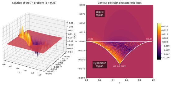
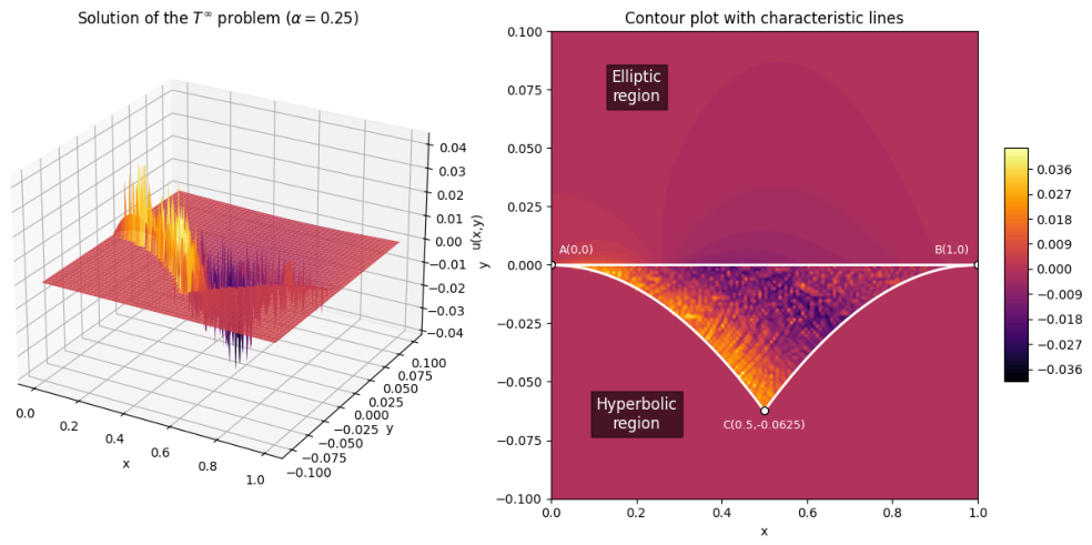
Figure 1 shows the numerical solution $u(x,y)$ of problem $T^{\infty }$ for the above parameters.

Figure 1. Surface and contour plot of the solution ($\alpha =0.25$).

The solution surface is smooth; in the hyperbolic region ($y<0$) the boundary condition $u=\psi$ on the characteristic $AC$ and $u=0$ on $BC$ are satisfied. In the elliptic part ($y>0$), the solution is positive in the central zone and decays monotonically to zero as $y\to \infty$ and on the vertical walls. Qualitatively, the picture corresponds to the perturbation potential in the subsonic region of a Laval nozzle with a continuous transition through the sonic line $y=0$.

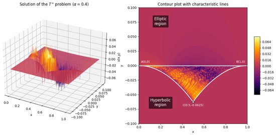
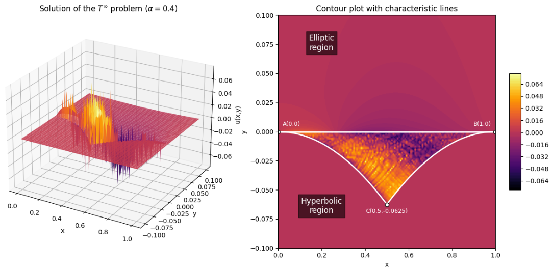
In Figure 2 the numerical solution of problem $T^{\infty }$ for $\alpha =0.4$ is shown. Compared with the case $\alpha =0.25$ (Figure 1), the larger value of $\alpha$ leads to several qualitative changes. In the elliptic part ($y>0$) the maximum of $u(x,y)$ is noticeably lower, the region where the solution is positive becomes narrower, and the decay to zero as $y\to \infty$ and on the vertical walls $x=0,1$ is steeper. This behavior is a consequence of the stronger dissipative effect of the term $\alpha u_y$ in the equation. In the hyperbolic part ($y<0$) the general shape of the solution remains similar, but the spatial distribution is modified: the maximum value of u becomes somewhat larger than for $\alpha =0.25$, while the solution on the characteristic $AC$ stays unchanged because it is fixed by the boundary condition $\psi \left(x\right)$. The overall picture remains physically consistent with the perturbation potential in the subsonic section of a Laval nozzle, showing more intense vertical damping for the larger $\alpha$.

Figure 2. Surface and contour plot of the solution ($\alpha =0.4$).

The observed influence of $\alpha$ admits a clear physical interpretation within the framework of transonic gas dynamics. The term ${\alpha \left|y\right|}^{m-1}{u}_y$ in the governing equation models an additional vertical dissipation mechanism, which can be associated with effects of viscosity, thermal conductivity, or the specific shape of the nozzle in the hodograph plane. As $\alpha$ grows, the damping of perturbations in the subsonic region ($y>0$) becomes stronger, leading to a lower maximum and a faster decay of the disturbance downstream. In the supersonic region ($y<0$), the same change in $\alpha$ modifies the parameter $\beta$ (7) and, consequently, the weight functions in the integral representation of the solution; for a fixed boundary value $\psi \left(x\right)$ on the characteristic $AC$, this results in a less singular behavior near the sonic line and, therefore, in a higher peak of the perturbation potential. Thus, the parameter $\alpha$ acts as a quantitative measure of the dissipative intensity in the flow and controls the balance between the subsonic and supersonic parts of the transonic field.

Thus, the constructed solution fully satisfies all conditions of problem $T^{\infty }$ and clearly demonstrates the effectiveness of the proposed method.

7. Conclusions

In this paper, the Tricomi problem $T^{\infty }$ for a second-kind mixed-type equation with a lower-order term in an unbounded domain whose elliptic part is a vertical half-strip and the hyperbolic part is bounded by characteristics was investigated. The main results are as follows.

(1) A uniqueness theorem for the solution of problem $T^{\infty }$ was proved using the extremum principle for elliptic equations and the Zaremba–Giraud principle.

(2) Using Green’s function method, an explicit representation of the solution in the elliptic half-strip was obtained in the form of a rapidly convergent series, while in the hyperbolic region a generalized solution of class ${\mathbb{R}}_2$ was employed. The matching of these representations on the degeneracy line led to a singular integral equation, which was regularized by the Carleman–Vekua method and reduced to a Fredholm integral equation of the second kind with a weak singularity. The solvability of the latter follows from the proven uniqueness.

(3) Explicit analytic formulas for the normal derivative $\nu \left(x\right)$ and the trace $\tau \left(x\right)$ on the degeneracy line were derived, expressed in terms of hypergeometric functions.

(4) For the specific parameter values $m=1$, $\alpha =0.25$ and $\alpha =0.4$ with the boundary function $\psi \left(x\right)=x^{6/5}{(1/2-x)}^{6/5}$, numerical calculations were carried out and three-dimensional surface and contour plots of the solution were constructed (Figure 1 and Figure 2). The comparison of the two cases clearly shows the influence of the parameter $\alpha$ on the solution: increasing $\alpha$ leads to a lower maximum in the elliptic part, a narrower region of positive values, and a steeper decay to zero as $y\to \infty$ and on the vertical walls, which is fully consistent with the enhanced dissipative effect of the term $\alpha u_y$ in the equation.

(5) A physical interpretation of the graphs was given in the context of transonic gas dynamics. It was shown that the solution is continuous and smoothly crosses the sonic line, corresponding to the picture of shockless transonic flow in Laval nozzles. The observed dependence on $\alpha$ mimics the influence of additional dissipation mechanisms in the subsonic zone.

The obtained results can be applied to the mathematical modeling of transonic flows, and the proposed method for constructing Green’s functions for degenerate elliptic equations in a half-strip and regularizing singular integral equations is of independent theoretical interest.

References

- Lavrentiev, M.A.; Bitsadze, A.V. On the problem of equations of mixed type. Dokl. Akad. Nauk SSSR 1950, 70, 485–488. (In Russian) [Google Scholar]
- Bers, L. Mathematical Aspects of Subsonic and Transonic Gas Dynamics; Courier Dover Publications: Mineola, NY, USA, 2016. [Google Scholar]
- Frankl, F.I. Selected Works on Gas Dynamics; Nauka: Moscow, Russia, 1973. (In Russian) [Google Scholar]
- Chen, G.-Q.G. Partial differential equations of mixed type—Analysis and applications. Not. Am. Math. Soc. 2023, 70, 8–23. [Google Scholar]
- Smirnov, M.M. Equations of Mixed Type; American Mathematical Society: Providence, RI, USA, 1978. [Google Scholar]
- Repin, O.A. The Tricomi problem for an equation of mixed type in a domain whose elliptic part is a half-strip. Differ. Equ. 1996, 32, 571–574. [Google Scholar]
- Zunnunov, R.T. Tricomi problem for a mixed-type equation in an unbounded domain. Uzb. Math. J. 2001, 2, 39–43. (In Russian) [Google Scholar]
- Ovsyannikov, L.V. On the motion of a wedge-shaped profile at the speed of sound. Proc. Leningr. Air Force Eng. Acad. Named A.F. Mozhaisky 1950, 33, 25–51. (In Russian) [Google Scholar]
- Falkovich, S.V. On one case of solving the Tricomi problem. Transonic Gas Flows 1964, 1, 3–8. (In Russian) [Google Scholar]
- Karol, I.L. On a certain boundary value problem for an equation of mixed elliptic-hyperbolic type. Dokl. Akad. Nauk SSSR 1953, 88, 197–200. (In Russian) [Google Scholar]
- Ivashkina, G.A. On problems of Bitsadze–Samarskii type for the equation uxx+sign y|y|muyy = 0, 0 < m < 1. Differ. Equ. 1981, 17, 1078–1089. (In Russian) [Google Scholar]
- Podkletnova, S.V. Problem N for the Euler-Darboux equation with two degeneration lines in characteristic coordinates and a trivial coefficient for the derivative of the desired function with respect to the ordinate. Vestn. Samara Univ. Nat. Sci. Ser. 2026, 32, 167–191. [Google Scholar]
- Zunnunov, R.T.; Ergashev, A.A. The problem with shift for an equation of mixed type of the second kind in an unbounded domain. Vestn. KRAUNC Fiz.-Mat. Nauk. 2016, 1, 26–31. [Google Scholar]
- Zunnunov, R.T. A nonlocal problem for a generalized Trikomi equation with a spectral parameter in the unbounded domain. Vestn. KRAUNC Fiz.-Mat. Nauk. 2021, 35, 17–26. [Google Scholar]
- Zunnunov, R.T.; Parovik, R.I.; Ergashev, A.A. A Bitsadze–Samarskii-type problem for a second-kind mixed-type equation in a domain with a horizontal half-strip as its elliptic part. Mathematics 2026, 14, 487. [Google Scholar]
- Ruziev, M.; Parovik, R.; Zunnunov, R.; Yuldasheva, N. Non-local problems for the fractional order diffusion equation and the degenerate hyperbolic equation. Fractal Fract. 2024, 8, 538. [Google Scholar] [CrossRef] [Scilit]
- Zunnunov, R.T.; Bektosheva, S.A.; Parovik, R.I. Tricomi problem for a mixed-type equation of the second kind in a domain the elliptic part of which is the first quadrant of the plane. Vestn. KRAUNC Fiz.-Mat. Nauk. 2026, 54, 93–103. [Google Scholar] [CrossRef] [Scilit]
- Zarubin, A.N.; Chaplygina, E.V. The Tricomi problem for a difference–differential equation of mixed type in an unbounded domain. Russ. Math. 2022, 66, 53–60. [Google Scholar] [CrossRef] [Scilit]
- Ruziev, M.K.; Kazakbaeva, K.B. A nonlocal problem for a degenerate equation of elliptic type with a singular coefficient. Lobachevskii J. Math. 2024, 45, 3371–3378. [Google Scholar] [CrossRef] [Scilit]
- Ruziev, M.K.; Kazakbaeva, K.B. On a boundary value problem for the Holmgren equation with singular coefficients in a half-plane. Lobachevskii J. Math. 2025, 46, 6003–6008. [Google Scholar] [CrossRef] [Scilit]
- Mirsaburov, M.; Turaev, R.N. A problem in an unbounded domain with combined Tricomi and Frankl conditions on one boundary characteristic for one class of mixed-type equations. Russ. Math. 2023, 67, 34–46. [Google Scholar] [CrossRef] [Scilit]
- Samko, S.G.; Kilbas, A.A.; Marichev, O.I. Fractional Integrals and Derivatives: Theory and Applications; Gordon and Breach Science Publishers: Lausanne, Switzerland, 1993. [Google Scholar]
- Nakhushev, A.M. Fractional Calculus and Its Applications; FIZMATLIT: Moscow, Russia, 2003. [Google Scholar]
- Kilbas, A.A.; Srivastava, H.M.; Trujillo, J.J. Theory and Applications of Fractional Differential Equations; Elsevier: Amsterdam, The Netherlands, 2006. [Google Scholar]
- Bitsadze, A.V. Boundary Value Problems for Second Order Elliptic Equations; Elsevier: Amsterdam, The Netherlands, 2012. [Google Scholar]
- Lebedev, N.N. Special Functions and Their Applications; Prentice-Hall: London, UK, 1965. [Google Scholar]
- Dolgova, I.M.; Mel’nikov, I.A. Construction of Green’s functions and matrices for equations and systems of the elliptic type. J. Appl. Math. Mech. 1978, 42, 740–746. [Google Scholar]
- Morse, P.M.; Feshbach, H. Methods of Theoretical Physics. Part I; McGraw-Hill: New York, NY, USA, 1953. [Google Scholar]
- Muskhelishvili, N.I.; Radok, J.R.M. Singular Integral Equations: Boundary Problems of Function Theory and Their Application to Mathematical Physics; Courier Corporation: North Chelmsford, MA, USA, 2008. [Google Scholar]
- Mirsaburov, M.; Makulbay, A.B.; Mirsaburova, G.M. A combined problem with local and nonlocal conditions for a class of mixed-type equations. Bull. Karaganda Univ. Math. Ser. 2025, 2, 163–176. [Google Scholar] [CrossRef] [Scilit]
- Gil, A.; Segura, J.; Temme, N.M. Noniterative computation of Gauss–Jacobi quadrature. SIAM J. Sci. Comput. 2019, 41, A668–A693. [Google Scholar]
- Gil, A.; Segura, J.; Temme, N.M. Fast and reliable high-accuracy computation of Gauss–Jacobi quadrature. Numer. Algorithms 2021, 87, 1391–1419. [Google Scholar]
- Van Horn, B.M.; Nguyen, Q. Hands-On Application Development with PyCharm: Build Applications Like a Pro with the Ultimate Python Development Tool; Packt Publishing Ltd.: Birmingham, UK, 2023. [Google Scholar]
- Shaw, Z.A. Learn Python the Hard Way; Addison-Wesley Professional: Carrollton, TX, USA, 2024. [Google Scholar]
Disclaimer/Publisher’s Note: The statements, opinions and data contained in all publications are solely those of the individual author(s) and contributor(s) and not of MDPI and/or the editor(s). MDPI and/or the editor(s) disclaim responsibility for any injury to people or property resulting from any ideas, methods, instructions or products referred to in the content. |
© 2026 by the authors. Licensee MDPI, Basel, Switzerland. This article is an open access article distributed under the terms and conditions of the Creative Commons Attribution (CC BY) license.