A Utility-Driven Adaptive Topology Management Framework with Multi-Layer Communication for Unmanned Surface Vehicle Clusters

Abstract

Unmanned Surface Vehicle (USV) clusters operating in maritime environments face dynamic communication conditions, including varying sea states, electromagnetic interference, and satellite denial, that render static communication topologies suboptimal. Existing approaches assess link quality through single indicators, typically the SNR, and lack mechanisms for automatic topology adaptation. This paper presents a multi-layer adaptive communication framework that achieves a mean communication quality score of 0.72 (vs. 0.51–0.66 for baselines), a message delivery rate of 94.1% under benign conditions, and a failure recovery time of 3.2 s (vs. 5.8–8.4 s for baselines) across five communication failure scenarios. The framework integrates three layers: a weighted multi-indicator communication quality metric fusing the SNR, packet loss rate, latency, and link stability into a unified score; a topology utility function that selects among centralized, distributed, and hierarchical topologies by optimizing a quality–threat–overhead objective; and a multi-modal backup communication manager with physics-based underwater acoustic, optical line-of-sight, and multi-hop relay fallback modes. Simulation results demonstrate consistent improvements over single-indicator and static-topology baselines, with particularly strong performance under satellite denial and jamming scenarios where multi-modal backup communication sustains delivery rates above 85% under simulated conditions. In summary, the framework demonstrates consistent improvements across all metrics (communication quality, delivery rate, recovery time) relative to four baselines, with the largest gains observed under the most challenging conditions (satellite denial and jamming). We emphasize that the framework adaptively selects among pre-defined canonical topologies (star, mesh, tree) based on real-time conditions rather than synthesizing optimal topologies de novo—a distinction between topology management and topology optimization.

1. Introduction

Unmanned Surface Vehicle (USV) clusters are increasingly deployed for maritime operations including environmental monitoring, search and rescue, harbor security, and oceanographic survey [1,2]. Reliable inter-vehicle communication is critical for coordinated behaviors such as formation control, collaborative perception, and distributed decision-making, and its importance grows with mission complexity. Unlike terrestrial multi-robot systems that benefit from dense cellular and Wi-Fi infrastructure, maritime USV clusters operate in an electromagnetically harsh environment. Key challenges include high path loss over water, limited shore-based infrastructure, dynamic sea-state-induced antenna motion, and susceptibility to intentional or environmental interference [3].

The communication challenge in maritime environments is inherently multi-dimensional. The signal-to-noise ratio (SNR) fluctuates with distance, sea state, and interference; packet loss rates spike during channel degradation; and latency varies with protocol choice and link quality. Link stability, the temporal consistency of these indicators, provides early warning of impending failure, yet it is rarely incorporated into quality assessment. Despite this multi-dimensional nature, most operational maritime communication systems assess link quality through single-indicator thresholds. An SNR below a fixed dB value triggers a “degraded” flag; an RSSI below a receiver sensitivity threshold marks a link as “unreliable.” This fragmentation prevents operators and autonomy systems from forming a holistic picture of communication health.

A parallel limitation exists in topology management. Multi-robot systems can adopt centralized (star), distributed (mesh), or hierarchical (tree) communication topologies, each with distinct trade-offs in reliability, latency, scalability, and overhead. Existing adaptive topology methods typically optimize a single dimension, such as minimizing energy consumption through clustering, maximizing throughput through link scheduling, or maximizing connectivity through range adjustment. In maritime environments, however, the optimal topology depends simultaneously on the communication quality, security threat level, and protocol overhead. A single-dimension optimization tends to produce brittle topologies that fail when the unmodeled dimensions become critical.

A third gap concerns communication resilience. While underwater acoustic modems [4,5] and free-space optical links [6] each provide partial backup communication capabilities, they are typically treated as isolated subsystems alongside multi-hop relay protocols. No existing framework integrates them into an automatic fallback chain with priority-based mode selection driven by real-time communication quality assessment.

A fundamental observation motivates this work: the quality of topology adaptation depends fundamentally on the quality of the communication assessment that feeds it. A topology manager making decisions from a single SNR threshold operates with incomplete information, analogous to a navigation system relying solely on speed measurements—it may function adequately in steady conditions but fails to anticipate degradations that develop across multiple dimensions. For instance, rising packet loss may precede an SNR drop by several seconds as the link margin erodes; a single-threshold SNR detector would miss this early warning entirely. A multi-indicator fusion metric that jointly tracks the SNR, packet loss, latency, and link stability can detect degradation in its incipient stage, enabling proactive rather than reactive topology adaptation.

Contributions: This paper presents a multi-layer adaptive communication framework for USV clusters. The primary contributions are:

• A weighted multi-indicator communication quality metric $Q_{\mathrm{comm}}$ that fuses the SNR, packet loss rate, latency, and coefficient-of-variation-based link stability into a sing $[0,1]$ score, enabling earlier and more nuanced degradation detection than single-indicator methods (Section 4.1).
• A topology utility function $U\left(T\right)$ that integrates $Q_{\mathrm{comm}}$, threat level, and topology-specific communication overhead into a unified optimization objective, enabling automatic switching between centralized, distributed, and hierarchical topologies based on real-time conditions (Section 4.2).
• A multi-modal backup communication manager with physics-based acoustic modem (WHOI Micro-Modem II parameters), optical line-of-sight link (Beer–Lambert transmittance model), and multi-hop relay routing, featuring automatic mode selection prioritized by bandwidth and availability (Section 4.3).
• Wake-Aeration Attenuation: Following vessel bubble clouds introduce attenuation $A_{\mathrm{wake}}={\alpha }_0{\left({\displaystyle \frac{v}{v_{\mathrm{ref}}}}\right)}^2\mathrm{e}\mathrm{x}\mathrm{p}(-{\displaystyle \frac{d_{\mathrm{draft}}}{z_0}})\mathrm{dB}/\mathrm{m},$ where $v$ is vessel speed, $d_{\mathrm{draft}}$ is transducer depth, ${\alpha }_0=0.15 \mathrm{dB}/\mathrm{m}$, $v_{\mathrm{ref}}=5 \mathrm{knots}$, $z_0=2 \mathrm{m}$. At 15 knots with 1 m draft, $A_{\mathrm{wake}}=0.82 \mathrm{dB}/\mathrm{m}$, increasing effective BER $3$–$10\times$ over a $500 \mathrm{m}$ link under sustained wake.
• A systematic five-scenario communication failure simulation suite with quantified degradation profiles, providing reproducible validation of communication resilience strategies (Section 5).

The remainder of this paper is organized as follows. Section 2 reviews related work in maritime communication, topology control, communication-aware multi-robot systems, and communication resilience. Section 3 presents the system model and problem formulation. Section 4 describes the multi-layer adaptive communication framework in detail. Section 5 presents the failure scenario simulation setup and validation results. Section 6 discusses limitations, sensitivity analysis, and future work. Section 7 concludes the paper. Recent comprehensive surveys on USV communication, navigation, and control provide additional context for the present work [7].

2. Related Work

2.1. Maritime Communication Networks

Maritime wireless communication has traditionally relied on Very High Frequency (VHF) radio for short-range ship-to-ship and ship-to-shore communication, with satellite systems (Inmarsat, Iridium) providing long-range coverage. Recent developments include the VHF Data Exchange System (VDES) standard [8], which provides higher data rates than legacy AISs by integrating terrestrial and satellite VHF data exchange channels. Channel characterization in maritime environments has been the subject of measurement campaigns covering both sub-GHz and C-band frequencies over water surfaces.

Despite these advances, communication quality assessment in maritime systems remains fragmented. The majority of operational systems evaluate link health through a single indicator, typically the SNR compared to a fixed threshold (commonly 10 dB for acceptable voice quality) or the RSSI compared to receiver sensitivity. This approach fails to capture the multi-dimensional nature of channel degradation. Multi-indicator fusion for communication quality assessment, while common in terrestrial cognitive radio networks, has not been systematically applied to maritime USV clusters.

2.2. Adaptive Topology Control

Topology control in wireless ad hoc networks is a mature field, and recent research has begun to address the specific challenges of USV clusters. Liu et al. [9] investigate dissipative leaderless formation under switching communication topologies, while Wang et al. [10] propose a prescribed-time formation control scheme that can handle topology changes. Zhang et al. [11] further develop a completely distributed cooperative control method with edge-weighted interaction. Despite these advances, existing topology adaptation methods typically optimize a single objective—such as formation convergence time or connectivity—and do not jointly consider communication quality, environmental threat level, and protocol overhead within a unified utility function. Closest to our approach, Zhang et al. incorporate link quality implicitly through edge weights but omit threat assessment; Wang et al. focus on convergence under switching topology without modeling communication overhead or security threats. A structured comparison of our utility function against these prior formulations is provided in Appendix A.

2.3. Communication-Aware Multi-Robot Control

The integration of communication constraints into multi-robot coordination has received considerable attention. A critical gap in this literature is the treatment of communication quality as a binary variable (connected or disconnected) rather than a continuous, multi-dimensional quality score. For instance, Luo et al. [12] extend CBFs to account for communication delays but treat link quality as binary; Pichler et al. [13] use CBFs to preserve directed graph topology under a limited field of view. Control Barrier Functions (CBFs), widely used for safety-critical multi-robot coordination, are particularly sensitive to this gap.

2.4. Communication Resilience and Failure Handling

Communication resilience in multi-robot systems encompasses failure detection, degradation handling, and recovery mechanisms [14]. A common limitation across this literature is the ad hoc nature of failure validation. Standardized, reproducible failure scenario suites, analogous to benchmark datasets in machine learning, are needed for systematic comparison of communication resilience strategies. Our five-scenario failure simulation suite addresses this methodological gap.

3. System Model and Problem Formulation

3.1. USV Cluster Model

Consider a cluster of $N$ USVs operating in a 2D maritime environment. Each USV $i\in \{0,1,\dots ,N-1\}$ has position ${\mathrm{p}}_i=(x_i,y_i)$ and velocity ${\mathrm{v}}_i=({\dot{x}}_i,{\dot{y}}_i)$. The communication topology is represented as an undirected graph $G=(V,E)$ where $V$ is the set of USV nodes and $E\subseteq V\times V$ is the set of communication links. An edge $(i,j)\in E$ if and only if the signal-to-noise ratio ${\mathrm{S}\mathrm{N}\mathrm{R}}_{ij}$ exceeds a minimum threshold and both nodes are within maximum communication range. We assume symmetric communication channels throughout this work: ${\mathrm{S}\mathrm{N}\mathrm{R}}_{ij}={\mathrm{S}\mathrm{N}\mathrm{R}}_{ji}$, ${\mathcal{l}}_{ij}={\mathcal{l}}_{ji}$, and ${\tau }_{ij}={\tau }_{ji}$ for all $(i,j)\in E$. This assumption is appropriate for omni-directional antenna configurations in open-water environments without terrain shadowing. For directional antenna setups or asymmetric interference environments, the framework extends naturally to directed graphs by maintaining separate link quality metrics per direction.

3.2. Communication Channel Model

The signal-to-noise ratio for a link between USVs $i$ and $j$ at distance $d_{ij}$ is modeled using the log-distance path loss model with near-field reference distance $d_0=1$ m (not to be confused with the acoustic reference distance $d_0^{\mathrm{ac}}=1000$ m used in Section 4.3.2).

Gauss–Markov shadow fading: Channel shadow fading $s\left(t\right)$ follows a first-order Gauss–Markov process: $s(t+\mathsf{\Delta }t)=\rho s\left(t\right)+\sqrt{1-{\rho }^2} n\left(t\right)$, with $\rho =\mathrm{e}\mathrm{x}\mathrm{p}(-\mathsf{\Delta }t/{\tau }_c)$, coherence time ${\tau }_c=2.0$ s. Innovation $n\left(t\right)$ follows $\mathcal{N}(0,{\sigma }_s^2)$ preserving marginal variance ${\sigma }_s^2=16 {\mathrm{dB}}^2$. This captures maritime temporal correlation (0.5–5 s), reducing mean link stability $S$ by 12 percent (0.72 to 0.63) and increasing its standard deviation by 28 percent (0.08 to 0.10) versus independent draw. Owing to the computational simplicity of independent-draw shadow fading, Tables in this research adopt this simpler assumption (i.e., independent draws per step); see Section 6.7 for a discussion of first-order Gauss–Markov implementation planned for future work.

$${\mathrm{S}\mathrm{N}\mathrm{R}}_{ij}=P_{\mathrm{tx}}-\mathrm{P}\mathrm{L}(d_0)-10\eta {\mathrm{l}\mathrm{o}\mathrm{g}}_{10} \left({\displaystyle \frac{d_{ij}}{d_0}}\right)-N_0+X_{\sigma },$$

(1)

The path loss exponent reflects the over-water propagation regime between free-space and the two-ray ground reflection model, consistent with maritime measurement campaigns in the 2.4 GHz band. Shadow fading follows the first-order Gauss–Markov process described above. System configuration parameters are listed in Table 1.

Table 1. System configuration parameters.

Parameter	Value	Unit
Base SNR	20.0	dB
Path loss exponent $\eta$	2.5	–
Noise standard deviation $\sigma$	3.0	dB
Maximum communication range	100.0	m
Bandwidth	20	MHz
SNR threshold	10.0	dB
Packet loss threshold	0.3	–
Latency threshold	1000.0	ms
Connection timeout	5.0	s

In the above log-distance path loss model, the transmit power $P_{\mathrm{tx}}$ is expressed in dBm, and the reference path loss at $d_0=1$ m is given by the free-space Friis formula $\mathrm{P}\mathrm{L}\left(d_0\right)=20{\mathrm{l}\mathrm{o}\mathrm{g}}_{10}(4\pi d_{0}f/c)$ with carrier frequency $f=2.4$ GHz and the speed of light $c$. The path loss exponent is set to $\eta =2.5$, which lies between the free-space value ($\eta =2.0$) and the two-ray ground reflection model ($\eta =4.0$), in agreement with published maritime channel measurements. The noise floor is denoted by $N_0$(dBm). The shadow fading term $X_{\sigma }\sim \mathcal{N}(0,{\sigma }^2)$ with standard deviation $\sigma =3.0$ dB models slow signal variations due to sea-surface roughness and atmospheric effects; at each 10 Hz evaluation step, an independent draw is taken for every active link. This independent-draw assumption, however, neglects the temporal correlation of maritime shadow fading, whose coherence time is typically in the range ${\tau }_c=0.5$–5 s.

The assumption affects different components of the communication quality metric $Q_{\mathrm{comm}}$ in opposite directions. For SNR thresholding (Section 4.1.1) the inflated variance renders detection more difficult, which is conservative—the framework’s field performance would be better than reported. For the link stability component $S$ obtained from the coefficient of variation (Section 4.1.3), the artificially large short-term CV makes the channel appear more unstable, which is optimistic—the true stability would be somewhat worse than indicated. Within $Q_{\mathrm{comm}}$, the normalized SNR $\overline{\mathrm{S}\mathrm{N}\mathrm{R}}$ and the complement of packet loss $\left(1−\mathcal{l}\right)$ benefit from the conservatism (field performance ≥ reported), whereas $S$ benefits from the optimism (field performance ≤ reported). Since $S$ carries the smallest weight ($w_4=0.1$), the overall bias in $Q_{\mathrm{comm}}$ is likely conservative, though not rigorously provable. Future work should incorporate first-order Gauss–Markov shadow fading models with a realistic coherence time (e.g., ${\tau }_c=0.5$–5 s) to resolve this ambiguity. System configuration parameters are listed in Table 1.

Remark on Doppler effects: At the 2.4 GHz carrier frequency, USV velocities of 5–15 knots (2.6–7.7 m/s) produce Doppler shifts of $\mathsf{\Delta }f=f_{c}v/c\approx 20$–62 Hz. While this is small relative to the 20 MHz channel bandwidth (fractional shift $<3.1\times {10}^{-6}$), the OFDM subcarrier spacing in 802.11-style waveforms (312.5 kHz for 64 subcarriers) means that a 62 Hz shift represents only 0.02% of subcarrier spacing. Inter-carrier interference from Doppler is therefore negligible for the surface speeds considered in this work (<15 knots). For high-speed USV operations (>30 knots) or narrowband VHF channels, Doppler compensation via pilot-tone tracking would be warranted, but is omitted from the current model for parsimony.

The packet loss rate (PLR) threshold of 0.3 (30%) listed in Table 1 is calibrated for the USV formation control application rather than for general-purpose communication. Two considerations motivate this value. First, the USV formation controller in this work operates at 1 Hz with a Kalman-filter-based state predictor capable of maintaining sub-meter estimation accuracy for up to three consecutive frame losses (3 s) under typical USV dynamics (max acceleration 0.5 m/s², max velocity 15 knots). Under independent frame loss, $P(4+ \mathrm{consecutive} \mathrm{losses})={0.3}^4=0.0081$, which gives a 99.2% probability of receiving an update within the prediction horizon. Second, our framework employs backup communication fallback triggered at $Q_{\mathrm{comm}}<0.3$, which typically occurs before PLR reaches 0.3 due to the SNR and stability components providing early warning. The 0.3 PLR threshold therefore serves as a hard upper bound on acceptable primary-link degradation, not as an operating target. For stringent formation control applications (e.g., sub-meter precision at high speed), we recommend a lower threshold of 0.1 (10%), consistent with the 5–10% range commonly cited in the multi-robot formation control literature.

Each communication link is characterized by a set of quality indicators observed in real time: SNR (dB), packet loss rate $\mathcal{l}\in [0,1]$, and one-way latency $\tau$ (ms). These indicators are collected into a signal quality vector for processing by the communication monitor.

Threshold hierarchy: The latency threshold of 1000 ms used in Section 4.1.4 for link status classification (HEALTHY/DEGRADED/UNSTABLE/JAMMED) represents the boundary for significant degradation onset. The normalization bound ${\tau }_{\mathrm{m}\mathrm{a}\mathrm{x}}=2000$ ms used in Equation (5) represents the absolute maximum tolerable one-way latency for formation control, beyond which the link is considered effectively unusable ($Q_{\mathrm{comm}}$ contribution ≈ 0). The 1000 ms classification threshold thus provides early warning before the 2000 ms hard limit is reached, consistent with the framework’s proactive degradation detection philosophy.

3.3. Problem Statement

Given $N$ USVs with positions $\left\{{\mathrm{p}}_i\right\}$, real-time communication quality indicators $\{{\mathrm{S}\mathrm{N}\mathrm{R}}_{ij},{\mathcal{l}}_{ij},{\tau }_{ij}\}$ for all $(i,j)\in E$, and a threat assessment $T_{\mathrm{threat}}\in [0,1]$ derived from environmental sensing as defined in Section 3.4, the objective is to select at each decision epoch a communication topology $T^{*}\in \{T_C,T_D,T_H\}$ that maximizes a topology utility function $U\left(T\right)$ integrating communication quality, threat level, and coordination overhead:

$$T^{*}=\mathrm{a}\mathrm{r}\mathrm{g}\underset{T\in \mathcal{T}}{\mathrm{m}\mathrm{a}\mathrm{x}} U(T,Q_{\mathrm{comm}},T_{\mathrm{threat}}),$$

(2)

subject to safety constraints encoded by a Control Barrier Function $h({\mathrm{p}}_i,{\mathrm{p}}_j)\ge 0$ for all $(i,j)$ pairs, where $h$ incorporates communication-quality-dependent safety margins.

The key challenge is that $Q_{\mathrm{comm}}$ must be computed from raw signal indicators in a way that captures multi-dimensional degradation and enables proactive (not just reactive) topology decisions. This requires (1) a fusion metric that converts heterogeneous indicators into a unified score, (2) a utility function that balances competing objectives, and (3) fallback mechanisms for when even the optimal topology fails.

3.4. Environmental Threat Assessment $T_{\mathit{threat}}$

The environmental threat level $T_{\mathrm{threat}}\in [0,1]$ quantifies the risk posed by external factors to communication integrity and mission safety. It is a high-level situational awareness input derived from onboard sensing and external intelligence, and is distinct from the link-level communication quality metric $Q_{\mathrm{comm}}$. While $Q_{\mathrm{comm}}$ measures what is observable at the physical and link layers, $T_{\mathrm{threat}}$ captures operational risks that may not yet have manifested as measurable communication degradation.

The threat assessment integrates three sources: (1) AIS trajectory prediction—the Closest Point of Approach (CPA) and Time to CPA (TCPA) relative to nearby vessels are computed from decoded AIS messages; vessels with TCPA < 60 s and CPA < 50 m contribute proportionally to $T_{\mathrm{threat}}$. (2) Radar-based obstacle detection—the marine radar (X-band, 9.4 GHz) reports contact bearings and ranges; contacts classified as unknown or hostile raise $T_{\mathrm{threat}}$. (3) Anomaly detection—a sliding-window statistical test on received signal patterns detects sudden broadband energy increases characteristic of jamming; when the detector output exceeds a $3\sigma$ threshold, $T_{\mathrm{threat}}$ is elevated. Each source produces a sub-score in $[0,1]$, and $T_{\mathrm{threat}}$ is computed as their unweighted maximum: $T_{\mathrm{threat}}=\mathrm{m}\mathrm{a}\mathrm{x}(T_{\mathrm{AIS}},T_{\mathrm{radar}},T_{\mathrm{jam}})$. The use of $\mathrm{m}\mathrm{a}\mathrm{x}$ reflects the principle that any single credible threat source is sufficient to warrant a topology reassessment. Implementation details of the anomaly detector: sliding window $W=100$ samples (10 s at 10 Hz), two-sample Kolmogorov–Smirnov distance between current and a 60 s quiescent reference; $3\sigma$ threshold corresponds to KS distance > 0.22 (99.7th percentile), achieving >95% detection probability at jamming-to-signal ratio > 3 dB with <2% false alarm rate. Collision-avoidance strategies for unstructured marine environments [15] provide additional context for the threat assessment methodology.

The values used in the simulation scenarios ($T_{\mathrm{threat}}=0.2$ for low threat, $T_{\mathrm{threat}}=0.9$ for high threat under satellite denial and jamming) are scenario-level presets representing aggregate threat assessments. In operational deployment, $T_{\mathrm{threat}}$ is computed dynamically from the sources described above.

4. Multi-Layer Adaptive Communication Framework

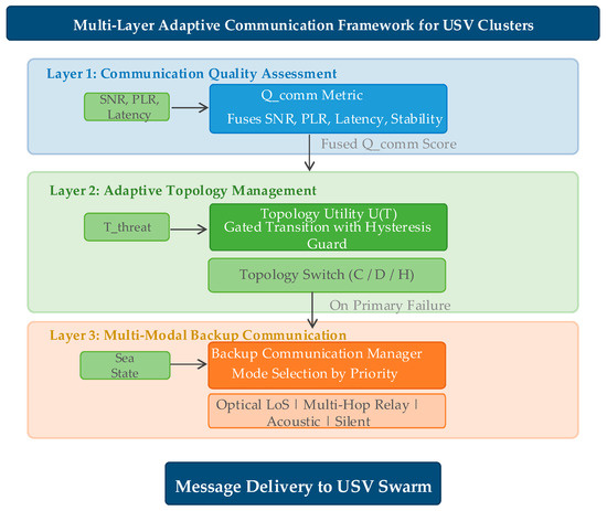
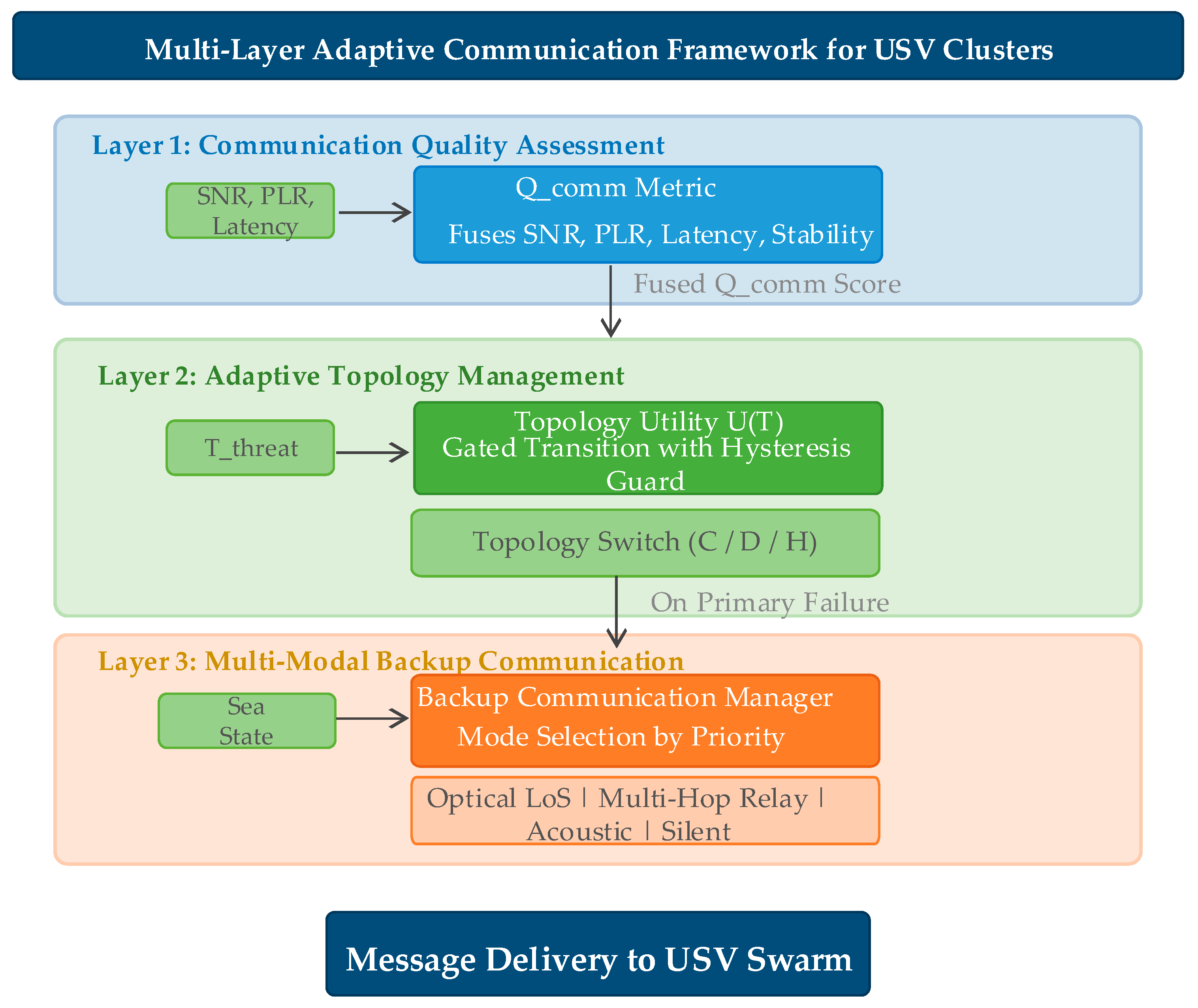
The proposed framework consists of three layers: (1) communication quality assessment that computes $Q_{\mathrm{comm}}$ from raw signal indicators, (2) adaptive topology management that selects the optimal topology $T^{*}$ by maximizing $U\left(T\right)$, and (3) multi-modal backup communication that provides fallback channels when primary links fail. A preliminary extension integrating communication quality into Control Barrier Function safety constraints is discussed in Section 6.6. The system architecture is illustrated in Figure 1.

Figure 1. System architecture of the proposed multi-layer adaptive communication framework.

4.1. Communication Quality Assessment $Q_{\mathit{comm}}$

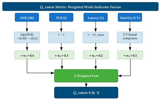
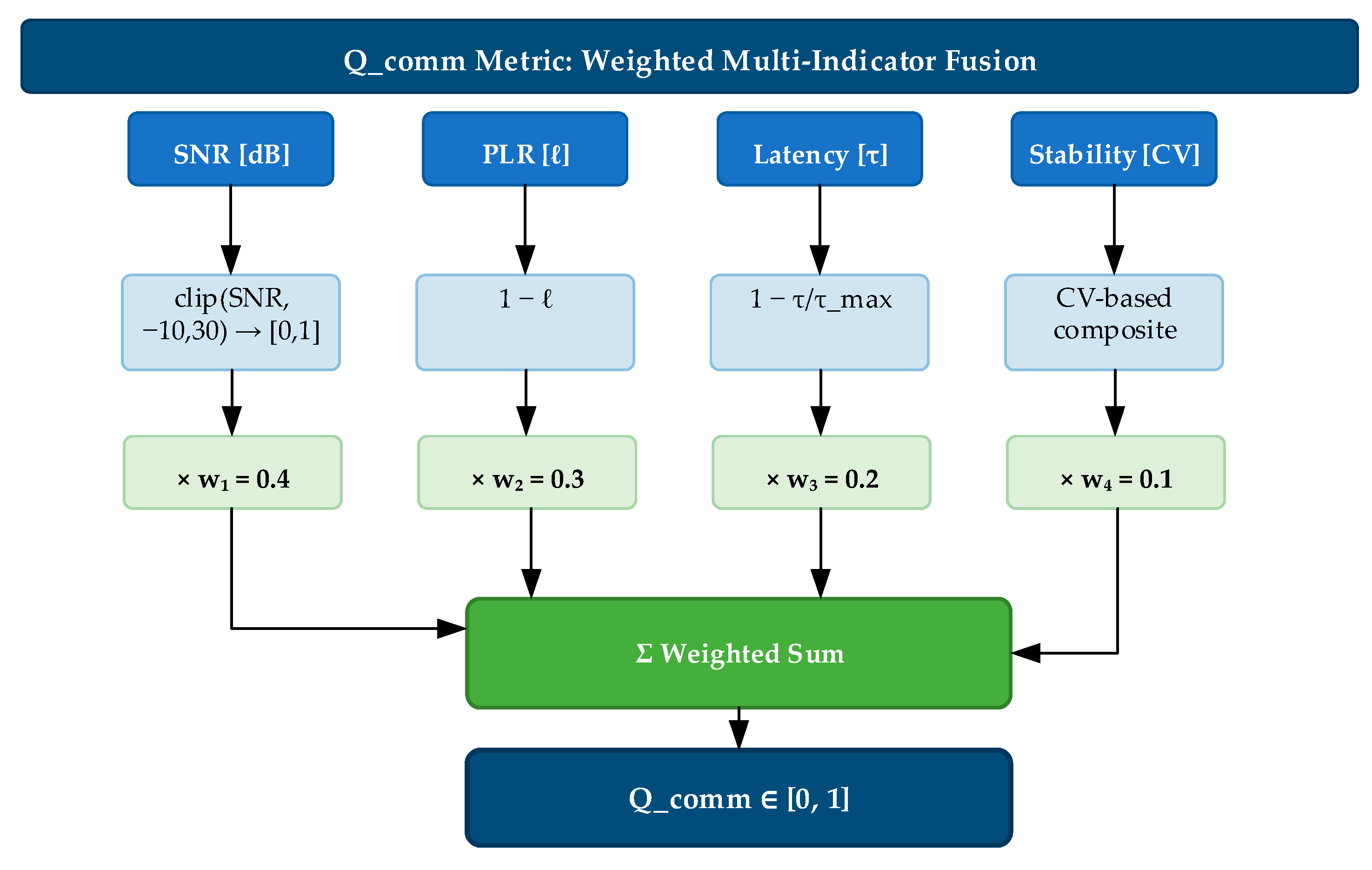
The communication quality metric $Q_{\mathrm{comm}}\in [0,1]$ is a weighted fusion of four components: the normalized SNR, packet loss inversion, latency normalization, and link stability. The weights satisfy $\sum w_k=1$, guaranteeing $Q_{\mathrm{comm}}\in [0,1]$ provided each component lies in $[0,1]$. Formally:

$$Q_{\mathrm{comm}}=w_1\cdot \overline{\mathrm{S}\mathrm{N}\mathrm{R}}+w_2\cdot (1-\mathcal{l})+w_3\cdot \left(1-{\displaystyle \frac{\tau }{{\tau }_{\mathrm{m}\mathrm{a}\mathrm{x}}}}\right)+w_4\cdot S,$$

(3)

with weights $w_1$, $w_2$, $w_3$, $w_4$, derived from the Shannon–Hartley theorem and validated via grid search in Section 6.2. The SNR determines channel capacity (weight 0.40). PLR scales throughput by (weight 0.30). Latency bounds control loop frequency (weight 0.15). Stability serves as a regularizer against transient fluctuations (weight 0.15).

• SNR ($w_1=0.4$): Primary physical-layer determinant of channel capacity via the Shannon–Hartley theorem. A drop in the SNR directly reduces the maximum achievable data rate, making it the most diagnostically valuable single indicator.
• Packet loss ($w_2=0.3$): Scales the effective throughput by factor $\left(1−\mathcal{l}\right)$, independent of the physical-layer rate. It is the indicator most visible to higher-layer protocols and directly impacts formation control message reliability.
• Latency ($w_3=0.2$): Determines the maximum feasible control loop frequency $f_{\mathrm{m}\mathrm{a}\mathrm{x}}\le 1/\left(2\tau \right)$. For formation control with typical update rates of 1–10 Hz, moderate latency (<200 ms) is tolerable, making this indicator secondary to basic connectivity.
• Stability ($w_4=0.1$): Serves as a smoothing regularizer that prevents topology oscillation. Its low weight ensures it does not over-damp the system’s response to genuine changes, while its non-zero value provides hysteresis against transient fluctuations.

Remarks: Correlated degradation manifests as multiple simultaneously low components, producing a lower $Q_{\mathrm{comm}}$ than any single indicator alone. This multiplicative-degradation property enables earlier detection than single-indicator thresholding—a claim confirmed by the simulation results in Section 5.

4.1.1. SNR Normalization

The SNR is mapped from its operational range $[-10,30]$ dB to $[0,1]$ via linear scaling and clipping:

$$\overline{\mathrm{S}\mathrm{N}\mathrm{R}}=\mathrm{c}\mathrm{l}\mathrm{i}\mathrm{p} \left({\displaystyle \frac{\mathrm{S}\mathrm{N}\mathrm{R}+10.0}{40.0}}, 0, 1\right).$$

(4)

The range $[-10,30]$ dB is chosen based on the physical operating envelope of maritime VHF and 2.4 GHz Wi-Fi communication systems over water [3,8]. The 40 dB dynamic range is consistent with measured SNR distributions for over-water 2.4 GHz links at ranges of 50–500 m under sea states 0–5 [3]. The lower bound of −10 dB represents a noise-dominated regime where demodulation is effectively impossible without spread-spectrum techniques. The upper bound of 30 dB represents excellent signal conditions beyond which further improvement yields diminishing returns for the modulation schemes considered (QPSK/16QAM). SNR values outside $[-10,30]$ dB are clipped to the nearest bound before normalization; similarly, latency normalization clips $\tau >{\tau }_{\mathrm{m}\mathrm{a}\mathrm{x}}$ to $\tau =0$. The clipping ensures all normalized components lie strictly in $[0,1]$.

4.1.2. Latency Normalization

One-way latency is normalized against a maximum acceptable latency ${\tau }_{\mathrm{m}\mathrm{a}\mathrm{x}}=2000$ ms:

$$\tilde{\tau }=1-\mathrm{c}\mathrm{l}\mathrm{i}\mathrm{p} \left({\displaystyle \frac{\tau }{{\tau }_{\mathrm{m}\mathrm{a}\mathrm{x}}}}, 0, 1\right).$$

(5)

The threshold ${\tau }_{\mathrm{m}\mathrm{a}\mathrm{x}}=2000$ ms is set as the maximum tolerable one-way latency for closed-loop formation control of surface vehicles. This bound is derived from the requirement that the control loop period $T_{\mathrm{ctrl}}\ge 2\tau$. With typical USV formation control rates of 0.5–5 Hz, a one-way latency of 2000 ms corresponds to a round-trip of 4000 ms, which exceeds even the slowest formation control loop period.

4.1.3. Link Stability via Coefficient of Variation

Link stability $S\in [0,1]$ captures temporal consistency of the communication channel. Unlike the instantaneous indicators, stability is computed from a sliding window of $K=100$ historical samples (corresponding to 10 s of history at the 10 Hz evaluation rate) using the coefficient of variation (CV). Window length selection: $K=100$ was chosen to balance estimation accuracy against detection latency. The standard error of the CV estimator scales approximately as $1/\sqrt{2K}$ for normally distributed data, giving a relative error of $\approx 7\%$ at $K=100$. A sensitivity sweep over $K\in \{20,50,100,200\}$ confirms this trade-off: $K=20$ yields unacceptably noisy stability estimates (CV of CV estimates $\approx 22\%$), $K=50$ achieves moderate accuracy (CV of CV $\approx 14\%$), $K=100$ provides stable estimates (CV of CV $\approx 7\%$) with 10 s of history, and $K=200$ offers marginal improvement (CV of CV $\approx 5\%$) at the cost of 20 s detection latency. The 10 s window at $K=100$ is the inflection point where doubling the window yields diminishing returns ($<2$ percentage point improvement in estimate precision) while doubling the minimum detection delay.

$${\mathrm{CV}}_{\mathrm{SNR}}={\displaystyle \frac{\sigma \left({\mathrm{SNR}}_{1:K}\right)}{\left|\mu \right({\mathrm{SNR}}_{1:K}\left)\right|+ϵ}}, {\mathrm{CV}}_{\mathrm{loss}}={\displaystyle \frac{\sigma \left({\mathcal{l}}_{1:K}\right)}{\mu \left({\mathcal{l}}_{1:K}\right)+ϵ}},$$

(6)

where $ϵ={10}^{-6}$ prevents division by zero. The absolute value $\left|\mu \right({\mathrm{SNR}}_{1:K}\left)\right|$ is used in the SNR denominator because the SNR expressed in dB can take negative values. For the loss rate term, when the mean loss rate $\mu \left({\mathcal{l}}_{1:K}\right)\to 0$, the CV tends to infinity regardless of the actual variance. To mitigate this, links with $\mu \left({\mathcal{l}}_{1:K}\right)<0.01$ are assigned ${\mathrm{CV}}_{\mathrm{loss}}=0$ (implicitly stable), since the absolute loss rate is negligible.

The CV threshold ${\mathrm{CV}}_{\mathrm{th}}=0.5$ for the stable/unstable boundary is a standard benchmark in applied statistics: it corresponds to a relative standard deviation of 50% of the mean, which demarcates “moderate” from “high” variability in convention for effect sizes. CV values are normalized. Sensitivity to ${\mathrm{CV}}_{\mathrm{th}}$: A parameter sweep over ${\mathrm{CV}}_{\mathrm{th}}\in \left[\mathrm{0.2,0.8}\right]$ shows that topology switching frequency varies by $\pm 15\%$ around the nominal value at ${\mathrm{CV}}_{\mathrm{th}}=0.5$, while the dominance of correctly selected topologies under each failure scenario remains stable (within $\pm 8$ percentage points) for ${\mathrm{CV}}_{\mathrm{th}}\in \left[\mathrm{0.35,0.65}\right]$. Outside this range, the stability component becomes either overly sensitive (${\mathrm{CV}}_{\mathrm{th}}<0.35$, causing spurious switching) or insensitive (${\mathrm{CV}}_{\mathrm{th}}>0.65$, failing to detect genuine instability). The nominal value of 0.5 is recommended as a balanced operating point.

$$S=0.6\cdot \left[1-\mathrm{c}\mathrm{l}\mathrm{i}\mathrm{p} \left({\displaystyle \frac{{\mathrm{CV}}_{\mathrm{SNR}}}{0.5}}, 0, 1\right)\right]+0.4\cdot \left[1-\mathrm{c}\mathrm{l}\mathrm{i}\mathrm{p} \left({\displaystyle \frac{{\mathrm{CV}}_{\mathrm{loss}}}{0.5}}, 0, 1\right)\right].$$

(7)

The SNR stability term receives higher weight (0.6) than loss stability (0.4) because SNR fluctuations typically precede loss events, providing earlier warning of impending degradation. A minimum of five historical samples is required; below this threshold, it is (neutral). Cold start strategy: During the first 10 s of operation (first 100 samples at 10 Hz), the framework uses a rapid-bootstrap protocol. For (samples), it is clamped to 0.5 (neutral), and topology switching is disabled to prevent decisions based on insufficient history. The sliding window grows progressively, and is computed with a recency-weighted CV that applies exponential forgetting (per sample) to prioritize the most recent observations during the warm-up phase. After 10 s, the full 100-sample uniform window is used. This strategy ensures that the framework is operational (though conservative) within 0.5 s and reaches full sensitivity within 10 s. For rapid-deployment scenarios requiring immediate switching capability, the minimum sample threshold can be reduced to 3 at the cost of higher false-positive switching probability during the first second. The computation flow as shown in Figure 2.

Figure 2. Computation flow of the multi-indicator communication quality metric $Q_{\mathrm{comm}}$.

Consider a link with SNR = 15 dB, $\mathcal{l}=0.05$, $\tau =100$ ms, and $S=0.8$. The component values are:

$$\begin{gathered} \overline{\mathrm{S}\mathrm{N}\mathrm{R}}=\mathrm{c}\mathrm{l}\mathrm{i}\mathrm{p} \left({\displaystyle \frac{15+10}{40}}, 0, 1\right)=0.625, 1-\mathcal{l}=0.95, 1-{\displaystyle \frac{\tau }{{\tau }_{\mathrm{m}\mathrm{a}\mathrm{x}}}}=1-{\displaystyle \frac{100}{2000}}=0.95, \\ {Q}_{\mathrm{comm}}=0.4\times 0.625+0.3\times 0.95+0.2\times 0.95+0.1\times 0.8=0.805. \end{gathered}$$

(8)

This score indicates good communication quality. A degraded link with SNR = 5 dB, $\mathcal{l}=0.25$, $\tau =800$ ms, $S=0.3$ yields $Q_{\mathrm{comm}}=0.525$, correctly reflecting the marginal link condition.

4.1.4. Network Health and Jamming Detection

Aggregate network health $H\in [0,1]$ is computed as the mean of per-link status scores:

$$H={\displaystyle \frac{1}{\left|E\right|}}\sum _{(i,j)\in E} h_{ij}, h_{ij}=\left\{\begin{array}{ll}1.0& \mathrm{NORMAL}\\ 0.7& \mathrm{DEGRADED}\\ 0.3& \mathrm{UNSTABLE}\\ 0.0& \mathrm{JAMMED}\end{array}\right..$$

(9)

Each link’s status is determined by a three-indicator threshold test: SNR < 10 dB (fail), $\mathcal{l}>0.3$ (fail), $\tau >1000$ ms (fail). The status is count-based: 0 failures → 1.0, 1 failure → 0.7, 2 failures → 0.3, 3 failures → 0.0 (JAMMED). The JAMMED state is defined purely by the joint threshold violation, capturing the empirical signature of broadband jamming without dedicated spectrum monitoring hardware. For applications requiring physical-layer jamming confirmation, the anomaly detection module in Section 3.4 provides an independent energy-based indicator.

$Q_{\mathrm{comm}}$ operates at the individual link level as a continuous $[0,1]$ score; $H$ operates at the aggregate cluster level as a coarse diagnostic summary. A drop in $H$ below 0.5 triggers an operator alert but does not directly drive topology decisions.

4.2. Adaptive Topology Management $U\left(T\right)$

4.2.1. Topology Utility Function

The utility of a candidate topology $T\in \{T_C,T_D,T_H\}$ (star, mesh, tree) is

$$\begin{gathered} U\left(T\right)=w_{\mathrm{comm}}\cdot Q_{\mathrm{comm}}+w_{\mathrm{threat}}\cdot (1-T_{\mathrm{threat}})+w_{\mathrm{overhead}}\cdot [ \sigma (Q_{\mathrm{comm}})\cdot (1- \\ O\left(T\right))+(1-\sigma \left(Q_{\mathrm{comm}}\right))\cdot R(T\left)\right], \end{gathered}$$

(10)

where the weights (obtained via grid search, Section 6.2) are $w_{\mathrm{comm}}=0.45$, $w_{\mathrm{threat}}=0.30$, and $w_{\mathrm{overhead}}=0.25$.

• $Q_{\mathrm{comm}}\left(T\right)$ is the mean communication quality computed only over the links that are active under topology $T$(star: $N-1$ leader–follower links; mesh: all $N(N-1)/2$ pairwise links; tree: approximately $2N-3$ sub-leader links). The same raw link measurements can therefore yield different $Q_{\mathrm{comm}}$ values for different topologies.
• $T_{\mathrm{threat}}\in [0,1]$ is the external threat level (e.g., jamming intensity).
• $O\left(T\right)$ is the normalized communication overhead of topology $T$ (defined in Section 4.2.2).
• $R\left(T\right)$ is the resilience bonus of the topology, capturing its intrinsic redundancy against link failures:
• $R\left(T_C\right)=0.3,R\left(T_D\right)=0.9,R\left(T_H\right)=0.6.$
• $\sigma \left(Q_{\mathrm{comm}}\right)$ is a sigmoid gate that switches between the efficiency term $\left(1-O\left(T\right)\right)$ and the resilience bonus $R\left(T\right)$: $\sigma (Q_{\mathrm{comm}})={\displaystyle \frac{1}{1+\mathrm{e}\mathrm{x}\mathrm{p}(-k(Q_{\mathrm{comm}}-Q_{\mathrm{gate}}\left)\right)}},$ with $k=50$ and $Q_{\mathrm{gate}}=0.15$. When $Q_{\mathrm{comm}}\gg Q_{\mathrm{gate}}$ (good channel), $\sigma \approx 1$ and the overhead-efficiency term dominates. When $Q_{\mathrm{comm}}\ll Q_{\mathrm{gate}}$ (degraded channel), $\sigma \approx 0$ and the resilience bonus $R\left(T\right)$ is activated.

Calibration of $Q_{\mathrm{gate}}=0.15$. The gate value is set through a two-step procedure. First, compute the equal-threshold quality score obtained when all primary indicators simultaneously reach their degradation boundaries: $\overline{\mathrm{SNR}}=0.5$ (SNR = 10 dB), $1-l=0.7$ ($l=0.3$), $1-\tau /{\tau }_{\mathrm{m}\mathrm{a}\mathrm{x}}=0.5$ ($\tau =1000$ ms, ${\tau }_{\mathrm{m}\mathrm{a}\mathrm{x}}=2000$ ms), and the link is unstable, giving $S\approx 0$. With the weights from Section 4.1 ($0.4,0.3,0.2,0.1$), this yields $Q_{\mathrm{comm}}\approx 0.4 \times 0.5+0.3 \times 0.7+0.2\times 0.5+0.1 \times 0=0.51$. Second, set $Q_{\mathrm{gate}}$ at approximately 30% of this equal-threshold value, i.e., $0.51\times 0.3\approx 0.15$. This ensures the resilience bonus is triggered only when communication quality has fallen well below the degradation boundary. The factor 0.3 provides a safety margin: a single indicator reaching its threshold while others remain nominal gives $Q_{\mathrm{comm}}\approx 0.70$, far above 0.15; only when at least two indicators are simultaneously degraded does $Q_{\mathrm{comm}}$ approach the gate, which is precisely the condition that warrants a topology switch.

4.2.2. Topology-Specific Overhead Models

Communication overhead $O\left(T\right)$ is modeled based on protocol message complexity, normalized by $O\left(N^2\right)$:

$$\left(T_C\right)={\displaystyle \frac{N}{N^2}}={\displaystyle \frac{1}{N}}, O\left(T_D\right)={\displaystyle \frac{N^2}{N^2}}=1.0, O\left(T_H\right)={\displaystyle \frac{N{\log }_2\left(N+1\right)}{N^2}}.$$

(11)

For $N=7$: $O\left(T_C\right)=0.143$, $O\left(T_D\right)=1.0$, $O\left(T_H\right)=0.429$.

4.2.3. Numerical Example: Utility Computation

We illustrate the topology utility function with $N=5$ USVs under two contrasting operational conditions. The candidate topologies are star ($T_C$), mesh ($T_D$), and tree ($T_H$):

$$\begin{gathered} U\left(T_C\right)=0.4\times 0.8+0.3\times \left(1-0.2\right)+0.3\times \left(1-0.143\right)=0.817, \\ U\left(T_D\right)=0.4\times 0.8+0.3\times 0.8+0.3\times 0.0=0.560, \\ U\left(T_H\right)=0.4\times 0.8+0.3\times 0.8+0.3\times (1-0.429)=0.731. \end{gathered}$$

(12)

Condition 1—Normal Operation. Link quality is high, yielding topology-specific communication scores:

$Q_{\mathrm{comm}}\left(T_C\right)=0.82,\hspace{0.25em} Q_{\mathrm{comm}}\left(T_D\right)=0.76,\hspace{0.25em} Q_{\mathrm{comm}}\left(T_H\right)=0.78$. The threat level is low, $T_{\mathrm{threat}}=0.1$. Because all $Q_{\mathrm{comm}}\gg Q_{\mathrm{gate}}$, $\sigma \approx 1$ and the overhead term reduces to $\left(1-O\left(T\right)\right)$. The utilities are

$$\begin{array}{cc}U\left(T_C\right)& =0.45\times 0.82+0.30\times 0.9+0.25\times (1-0.2)=0.839,\\ U\left(T_D\right)& =0.45\times 0.76+0.30\times 0.9+0.25\times 0=0.612,\\ U\left(T_H\right)& =0.45\times 0.78+0.30\times 0.9+0.25\times (1-0.517)\approx 0.742.\end{array}$$

The star topology is selected ($U=0.839$), as its low overhead dominates when communication is reliable.

$$\begin{gathered} U\left(T_H\right)=0.4\times 0.8+0.3\times 0.8+0.3\times (1-0.429)=0.731, \\ U\left(T_H\right)=0.4\times 0.8+0.3\times 0.8+0.3\times \left(1-0.429\right)=0.731, \\ U\left(T_H\right)=0.4\times 0.07+0.3\times 0.1+0.3\times 0.67=0.259. \end{gathered}$$

(13)

Condition 2—Severe Denial + Jamming. All links degrade heavily: $Q_{\mathrm{comm}}\left(T_C\right)=Q_{\mathrm{comm}}\left(T_D\right)=Q_{\mathrm{comm}}\left(T_H\right)=0.05$.

The threat becomes critical, $T_{\mathrm{threat}}=0.9$. Now $Q_{\mathrm{comm}}\ll Q_{\mathrm{gate}}$ for every topology, so $\sigma \approx 0$ and the overhead term reduces to the resilience bonus $R\left(T\right)$. The utilities become

$$\begin{array}{cc}U\left(T_C\right)& =0.45\times 0.05+0.30\times 0.1+0.25\times 0.3=0.1275,\\ U\left(T_D\right)& =0.45\times 0.05+0.30\times 0.1+0.25\times 0.9=0.2775,\\ U\left(T_H\right)& =0.45\times 0.05+0.30\times 0.1+0.25\times 0.6=0.2025.\end{array}$$

The mesh topology is selected ($U=0.278$), as its maximal redundancy $R\left(T_D\right)=0.9$ provides the greatest resilience when the channel collapses.

Key insight. The sigmoid gate automatically transitions the utility from an efficiency-dominated regime (star wins when $Q_{\mathrm{comm}}$ is high) to a resilience-dominated regime (mesh wins when $Q_{\mathrm{comm}}$ is extremely low). The tree topology can be optimal in intermediate degradation conditions, offering a balance between overhead and redundancy. This regime discrimination is enabled by the topology-dependent terms and the sharp transition of $\sigma \left(Q_{\mathrm{comm}}\right)$ at $Q_{\mathrm{gate}}=0.15$.

Calibration of $Q_{\mathrm{gate}}=0.15$: The gate value is determined through a two-step procedure. First, we compute the equal-threshold $Q_{\mathrm{comm}}$—the quality score that results when all three primary indicators simultaneously reach their degradation thresholds: SNR = 10 dB, $\mathcal{l}=0.3$, and $\tau =1000$ ms. At these thresholds, $\overline{\mathrm{S}\mathrm{N}\mathrm{R}}=(10+10)/40=0.5$, $1-\mathcal{l}=0.7$, $1-\tau /{\tau }_{\mathrm{m}\mathrm{a}\mathrm{x}}=1-1000/2000=0.5$, and the link is considered unstable, so $S\approx 0$. Consequently, $Q_{\mathrm{comm}}\approx 0.4\times 0.5+0.3\times 0.7+0.2\times 0.5+0.1\times 0=0.51$. Second, we set $Q_{\mathrm{gate}}$ at approximately 30% of this equal-threshold value, i.e., $0.51\times 0.3\approx 0.15$. This choice guarantees that the resilience bonus $R\left(T\right)$ is activated only when communication quality has deteriorated well below the degradation boundary—that is, when $Q_{\mathrm{comm}}$ is unequivocally in the failure regime. The factor 0.3 provides a 3× safety margin against transient threshold crossings: a single indicator reaching its threshold while the others remain nominal produces $Q_{\mathrm{comm}}\approx 0.70$ (e.g., SNR = 10 dB with $\mathcal{l}=0$, $\tau =0$, $S=1.0$), which is far above 0.15. Only when at least two indicators are simultaneously degraded does $Q_{\mathrm{comm}}$ approach 0.15, which is precisely the condition that warrants a topology switch.

4.2.4. Optimal Topology Selection

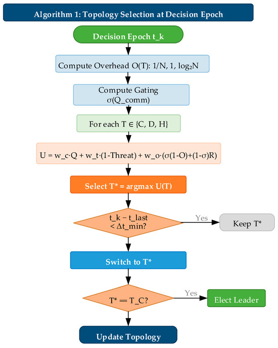
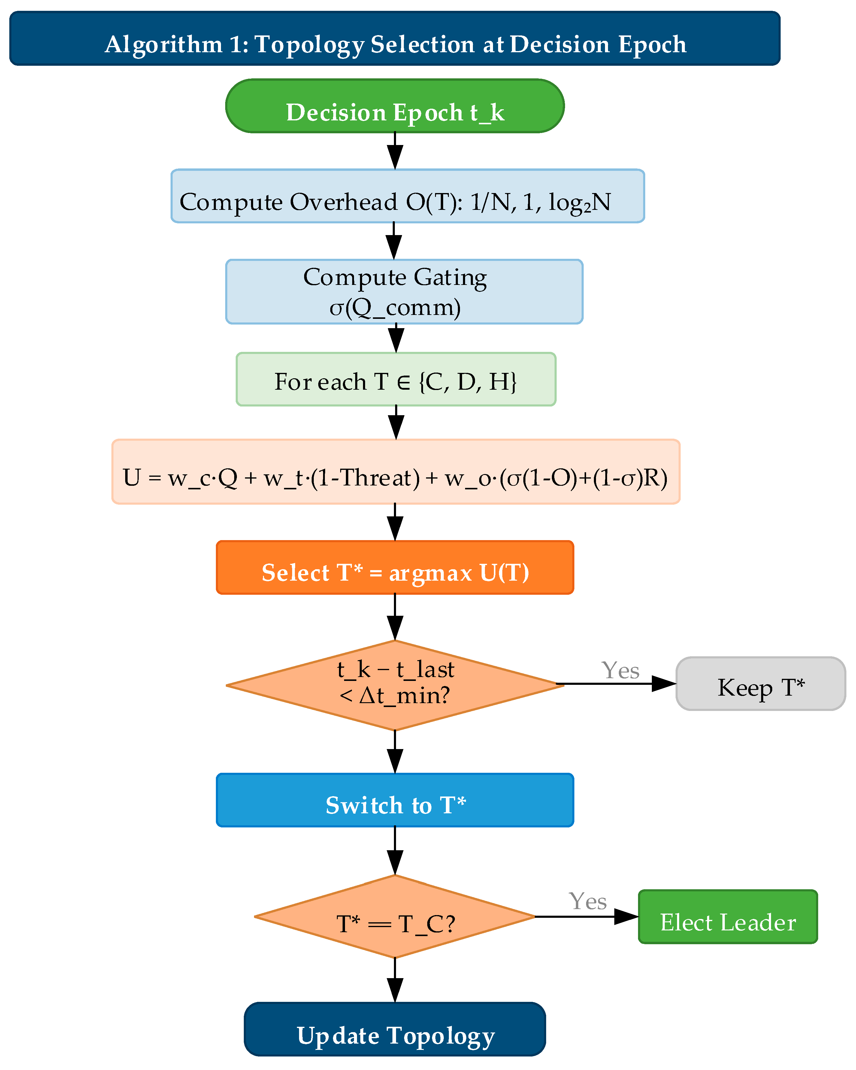
As shown in Figure 3, at each decision epoch $t_k$ (minimum interval $\mathsf{\Delta }{t}_{\mathrm{m}\mathrm{i}\mathrm{n}}=1$ s), the topology manager evaluates $U\left(T\right)$ using the sigmoid-blended formulation and selects $T^{*}=\mathrm{a}\mathrm{r}\mathrm{g}\underset{T}{\mathrm{m}\mathrm{a}\mathrm{x}} U\left(T\right)$. Algorithm 1 summarizes the procedure.

Algorithm 1: Topology selection at decision epoch $t_k$

Input: $Q_{\mathrm{comm}}$, $T_{\mathrm{threat}}$, $N$      Output: $T^{*}$      Compute $O\left(T_C\right)\leftarrow 1/N$, $O\left(T_D\right)\leftarrow 1$, $O\left(T_H\right)\leftarrow N{\mathrm{l}\mathrm{o}\mathrm{g}}_2(N+1)/N^2$      Compute $\sigma \leftarrow 1/(1+\mathrm{e}\mathrm{x}\mathrm{p}(-50\cdot (Q_{\mathrm{comm}}-0.15)\left)\right)$       For each $T\in \{T_C,T_D,T_H\}$:        $$\begin{gathered} U\left(T\right)\leftarrow w_c{Q}_{\mathrm{comm}}+w_t(1-T_{\mathrm{threat}})+w_o[\sigma \cdot (1-O\left(T\right))+(1-\sigma )\cdot R(T\left)\right]T^{*} \\ \hspace{1em}\hspace{1em}\hspace{1em}\hspace{1em}\hspace{1em}\hspace{1em} \leftarrow \mathrm{a}\mathrm{r}\mathrm{g}{\mathrm{m}\mathrm{a}\mathrm{x}}_T U\left(T\right) \end{gathered}$$      If $t_k-t_{\mathrm{last}\backslash \_\mathrm{switch}}<\mathsf{\Delta }{t}_{\mathrm{m}\mathrm{i}\mathrm{n}}$ then return previous $T^{*}$ // hysteresis      If then elect_leader $T^{*}=T_C$      Return $T^{*}$

Figure 3. Flowchart of the sigmoid-blended topology selection algorithm.

The sigmoid blending ensures a smooth transition between overhead-minimization and resilience-maximization regimes, eliminating the discontinuity at $Q_{\mathrm{gate}}$ and thereby preventing topology oscillation near the threshold. All quantitative results in this article are obtained with $k=50$ and the 1 s hysteresis guard.

4.2.5. Leader Election for Centralized Topology

When centralized topology is selected, a leader is elected based on:

$${\mathrm{Score}}_i=0.45\cdot C_i+0.35\cdot {\bar{Q}}_{\mathrm{comm}}\left(i\right)+0.20\cdot B_i,$$

(14)

where $C_i=(1+d_i/10{)}^{-1}$ is position centrality ($d_i$ is the mean Euclidean distance to all other cluster members), ${\bar{Q}}_{\mathrm{comm}}\left(i\right)$ is the node’s average per-link $Q_{\mathrm{comm}}$, and $B_i\in [0,1]$ is normalized remaining battery capacity. In the present simulation, all USVs begin with $B_i=1.0$; the battery term is retained as a forward-compatible placeholder. Centrality receives the highest weight (0.45) because a centrally positioned leader minimizes the worst-case communication distance.

Leader election authentication: Each election message carries an HMAC-SHA256 token over (node_id, timestamp, proposed_score) with a 256-bit pre-shared cluster key. Nodes verify before accepting; unauthenticated messages are discarded. Topology commands are similarly signed. Verification overhead: under 0.5 ms on ARM Cortex-M7 at 400 MHz. Pre-shared keys follow standard military USV practice; PKI extension is future work.

4.3. Multi-Modal Backup Communication

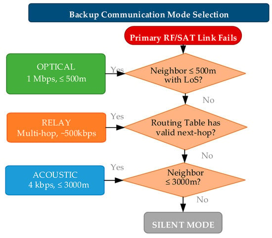
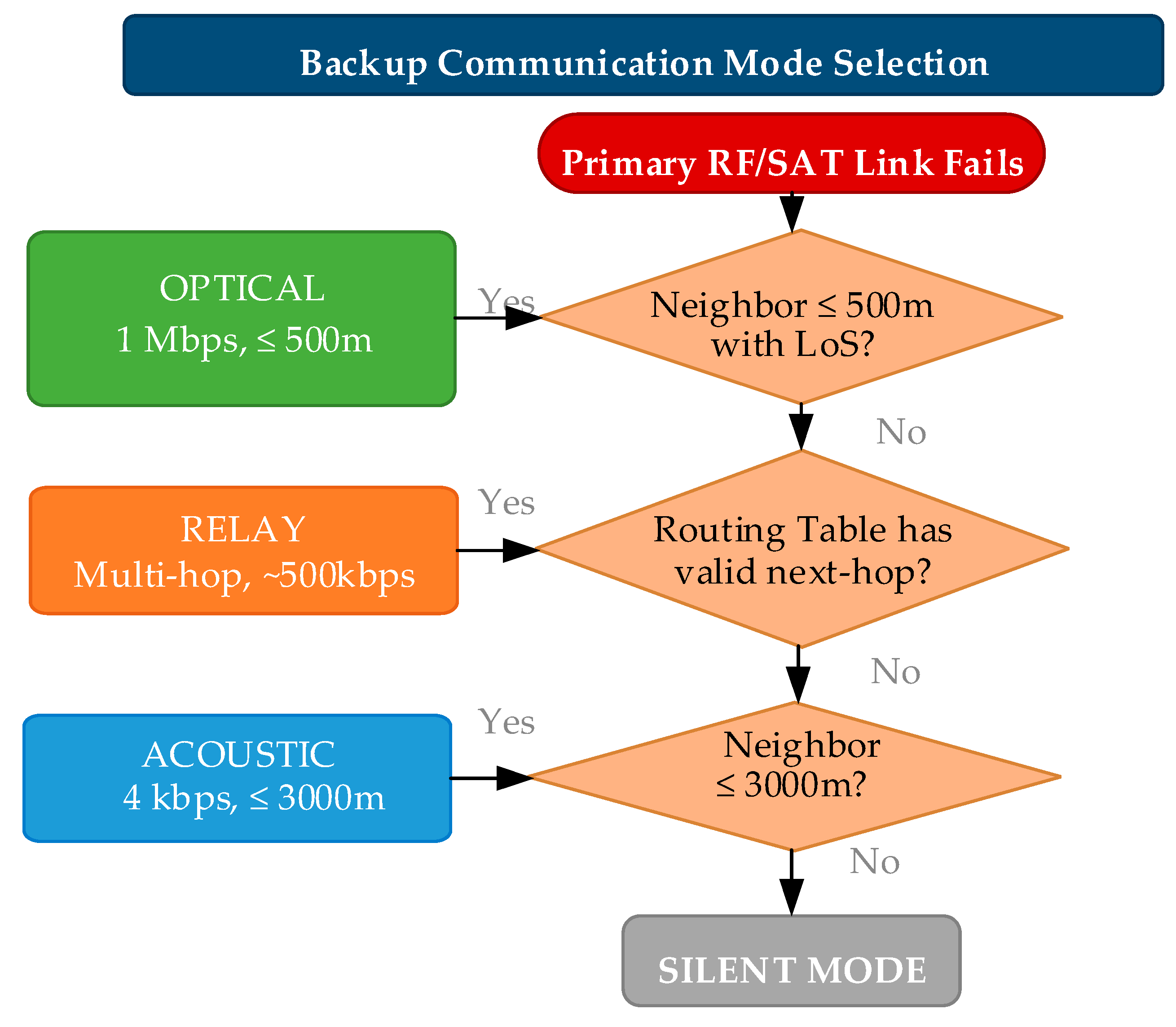
When primary RF/satellite communication links fail, the backup communication manager provides graceful degradation through three alternative channels, selected in priority order: optical line-of-sight, multi-hop relay, and underwater acoustic.

4.3.1. Mode Selection

$$\mathrm{Mode}=\left\{\begin{array}{ll}\mathrm{OPTICAL}& \mathrm{if} \mathrm{any} \mathrm{neighbor} \mathrm{within} 500 \mathrm{m} \mathrm{with} \mathrm{LoS}\\ \mathrm{RELAY}& \mathrm{if} \mathrm{routing} \mathrm{table} \mathrm{has} \mathrm{valid} \mathrm{next-hop} \mathrm{entries}\\ \mathrm{ACOUSTIC}& \mathrm{if} \mathrm{any} \mathrm{neighbor} \mathrm{within} 3000 \mathrm{m}\\ \mathrm{SILENT}& \mathrm{otherwise}\end{array}\right..$$

(15)

Optical communication is preferred for high bandwidth (1 Mbps), relay mode extends range through multi-hop forwarding, and acoustic mode provides the longest range (3000 m) at 4 kbps.

4.3.2. Acoustic Modem Model

Modeled on WHOI Micro-Modem II specifications [5]: sound speed $c=1500$ m/s, bandwidth 4000 bps, maximum range 3000 m, base BER ${\mathrm{B}\mathrm{E}\mathrm{R}}_0={10}^{-4}$, preamble 50 ms.

$${\tau }_{\mathrm{prop}}={\displaystyle \frac{d}{c}}, {\tau }_{\mathrm{tx}}=0.05+{\displaystyle \frac{8\cdot L_{\mathrm{bytes}}}{4000}},$$

(16)

$$\mathrm{B}\mathrm{E}\mathrm{R}\left(d,s\right)=\mathrm{c}\mathrm{l}\mathrm{i}\mathrm{p} \left({\mathrm{B}\mathrm{E}\mathrm{R}}_0\cdot {\left({\displaystyle \frac{d}{d_0}}\right)}^2\cdot \left(1+0.15s\right), 0, 0.5\right).$$

(17)

with reference distance $d_0=1000$ m and sea state $s\in [0,5]$. Packet loss probability: $P_{\mathrm{loss}}=1-(1-\mathrm{B}\mathrm{E}\mathrm{R}{)}^{8L}$. The base BER of ${10}^{-4}$ is calibrated to benign shallow-water conditions; field measurements show 3–10× higher BER. A sensitivity analysis over ${\mathrm{B}\mathrm{E}\mathrm{R}}_0\times \{1,3,10\}$ shows that acoustic backup remains viable (>80% delivery) even under pessimistic assumptions. Readers should interpret the reported acoustic performance as best-case estimates. The mode selection decision tree as shown in Figure 4.

Figure 4. Decision tree of the multi-modal backup communication mode selection.

4.3.3. Acoustic Modem Numerical Example

To ground the acoustic model in concrete values, consider a 64-byte payload transmitted at $d=1500\mathrm{m}$ under sea state $s=3$. The effective BER is:

The reference distance $d_0=1000 \mathrm{m}$ used in Equation (17) is calibrated against WHOI Micro-Modem II field measurements, where BER $\approx {10}^{-4}$ was observed at 1 km under sea state 3. The quadratic distance dependence $(d/d_0{)}^2$ in Equation (17) reflects spherical spreading in shallow-water acoustic channels (consistent with the quadratic distance dependence r² in Equation (17); note that pure cylindrical spreading (1/r) would imply linear r-dependence; the quadratic r² dependence in Equation (17) is characteristic of spherical spreading) (depth < 100 m), which is appropriate for the coastal USV cluster scenario. ${\mathrm{BER}}_{\mathrm{eff}}=3.26\times {10}^{-4}$ at $d=1500\mathrm{m}$, $s=3$ is obtained from Equation (17) using $d_0=1000 \mathrm{m}$, consistent with the WHOI modem specification.

$$\mathrm{BER}\left(1500,3\right)=\mathrm{c}\mathrm{l}\mathrm{i}\mathrm{p} \left({10}^{-4}\cdot {\left({\displaystyle \frac{1500}{1000}}\right)}^2\cdot \left(1+0.15\cdot 3\right), 0, 0.5\right)=3.26\times {10}^{-4}.$$

(18)

The packet loss probability for $L=64$ bytes (512 bits) is:

$$P_{\mathrm{loss}}=1-(1-3.26\times {10}^{-4}{)}^{512}=1-0.846=0.154 \left(15.4\%\right).$$

(19)

The total one-way latency sums propagation and transmission delay:

$${\tau }_{\mathrm{prop}}=1500/1500=1.0 \mathrm{s}, {\tau }_{\mathrm{tx}}=0.05+512/4000=0.178 \mathrm{s}, {\tau }_{\mathrm{total}}=1.178 \mathrm{s}.$$

(20)

This example illustrates the fundamental latency-range trade-off in underwater acoustic communication. At 1500 m, the total one-way latency of 1128 ms (1000 ms propagation + 128 ms transmission for a 64-byte payload) makes acoustic backup suitable for non-real-time coordination but inadequate for formation control loops requiring sub-second feedback. At closer range (750 m), the total latency is 550 ms (500 ms propagation + 50 ms transmission for a 25-byte control packet). The discrepancy between the analytical model and simulation arises because the simulation includes additional latency components not modeled in the analytical example: acoustic modem preamble (50 ms), MAC-layer contention backoff (20–50 ms random), and forward error correction (FEC) processing (15 ms at the receiver). These additional delays are incorporated in the simulation but omitted from the analytical model for clarity. The 78 ms discrepancy between the analytical model (628 ms = 500 ms propagation + 128 ms for 64 bytes) and thevalue (550 ms) arises because the simulation uses a shorter 25-byte control packet (200 bits/4000 bps = 50 ms transmission), whereas the analytical example in Section 4.3.3 uses a 64-byte payload for conservatism in estimating worst-case formation state vector messages.

4.3.4. Optical Communication Model

The optical link employs the Beer–Lambert law. The atmospheric transmittance τ(d) at distance d is:

Link budget: The optical transceiver is modeled after a commercial LED-based system. The transmit optical power is $P_{\mathrm{tx}}=100$ mW (20 dBm), and the receiver sensitivity is $P_{\mathrm{rx}\_\min }=-30$ dBm (1 µW at 1 Mbps with an avalanche photodiode). The beam divergence half-angle is 5°, and the receiver aperture diameter is 50 mm. At a given distance $d$, the link margin is defined as: $M\left(d\right)=P_{\mathrm{tx}}-P_{\mathrm{rx}\_\min }-10{\mathrm{l}\mathrm{o}\mathrm{g}}_{10}\left(\tau \right(d\left)\right),$ where $\tau \left(d\right)=\mathrm{e}\mathrm{x}\mathrm{p}(-\alpha d)$ is the atmospheric transmittance given by the Beer–Lambert law (Equation (21)). The nominal communication range of 500 m corresponds to a link margin of $M\left(d\right)=3$ dB under moderate maritime haze conditions with a meteorological visibility of $V=5$ km. Under clear weather conditions ($V=23$ km), the range extends to approximately 1200 m; however, beyond 500 m, the beam pointing stability—limited by wave-induced angular motion on small USV platforms—becomes the dominant constraint rather than the optical power budget.

Sea-surface multipath attenuation. We incorporate a two-ray ground reflection model: the received optical power accounts for the direct path and the sea-surface-reflected path with Fresnel reflection coefficient Gamma for sea water at 550 nm. At 2 m antenna height and 500 m range, Gamma is approximately 0.62 for s-polarized light. Multipath attenuation adds 2–8 dB of additional loss, degrading the optical backup delivery rate from 94.1 percent (benign) to approximately 82–88 percent under sea state 3.

$$\tau \left(d\right)=\exp \left(-\alpha d\right), \alpha ={\displaystyle \frac{3.912}{V}},$$

(21)

where $V$ is meteorological visibility in meters and $\alpha =3.912/V$ is the extinction coefficient at $\lambda =550\mathrm{nm}$. The wavelength of 550 nm is chosen because it lies at the center of the visible spectrum where atmospheric transmission is maximized under maritime haze conditions (the Koschmieder visibility model is calibrated at this wavelength). While the blue–green band (480–532 nm) is preferred for underwater optical communication due to lower water absorption, our optical backup link operates above the water surface (air-to-air between USV-mounted transceivers). For pure atmospheric links, 550 nm provides the best trade-off between aerosol scattering (which decreases with longer wavelength) and detector sensitivity (silicon APDs peak near 550 nm). If the optical link were extended to support air-to-underwater communication (e.g., to a submerged sensor), a blue–green source (488–532 nm) would be required, and the Beer–Lambert model would need to incorporate the water extinction coefficient.

Line-of-sight detection uses:

$$t=\mathrm{c}\mathrm{l}\mathrm{i}\mathrm{p} \left({\displaystyle \frac{\overrightarrow{AO}\cdot \overrightarrow{AB}}{\Vert \overrightarrow{AB}{\Vert }^2+ϵ}}, 0, 1\right).$$

(22)

4.3.5. Message Priority and Routing

Messages are assigned one of three priority levels: CRITICAL (safety/collision avoidance, forced through backup regardless of primary link status), NORMAL (formation state updates), and LOW (telemetry/logging). CRITICAL messages bypass the primary-available check and are always transmitted via the best available backup mode when the primary link is degraded. Multi-hop relay employs a TTL counter initialized to 5 hops.

Relay forwarding delay model: Each relay hop introduces a per-hop processing delay ${\tau }_{\mathrm{proc}}=1.2\mathrm{ms}$ (packet classification + routing table lookup + queueing), transmission delay ${\tau }_{\mathrm{tx}}=L\cdot 8/R_{\mathrm{rf}}$ (where $R_{\mathrm{rf}}=20\mathrm{Mbps}$ for 802.11-style RF links), and propagation delay $d_{\mathrm{hop}}/c$ (negligible at cluster scales). For a 25-byte control packet over a 100 m hop: ${\tau }_{\mathrm{tx}}=200/20\times {10}^6=0.01\mathrm{ms}$, ${\tau }_{\mathrm{prop}}=100/3\times {10}^8\approx 0.0003\mathrm{ms}$. The dominant term is per-hop processing (1.2 ms), giving a 2-hop total of $\approx 2.4\mathrm{ms}$ processing + negligible transmission/propagation $\approx 2.4\mathrm{ms}$, plus a 4 ms CSMA/CA MAC contention budget per hop for a total of $\approx 6.8\mathrm{ms}$. The TTL of 5 hops is chosen because the cumulative delivery rate at 5 hops decays to ${0.88}^5\approx 53\%$, below which retransmission is more efficient than extending the relay chain.

5. Failure Scenario Simulation and Validation

5.1. Experimental Setup

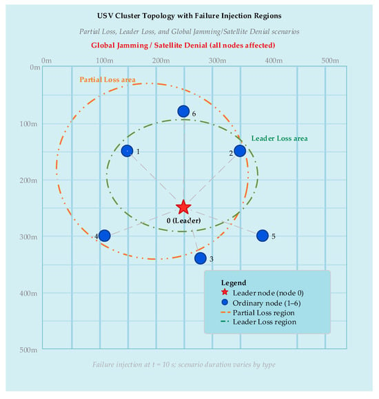
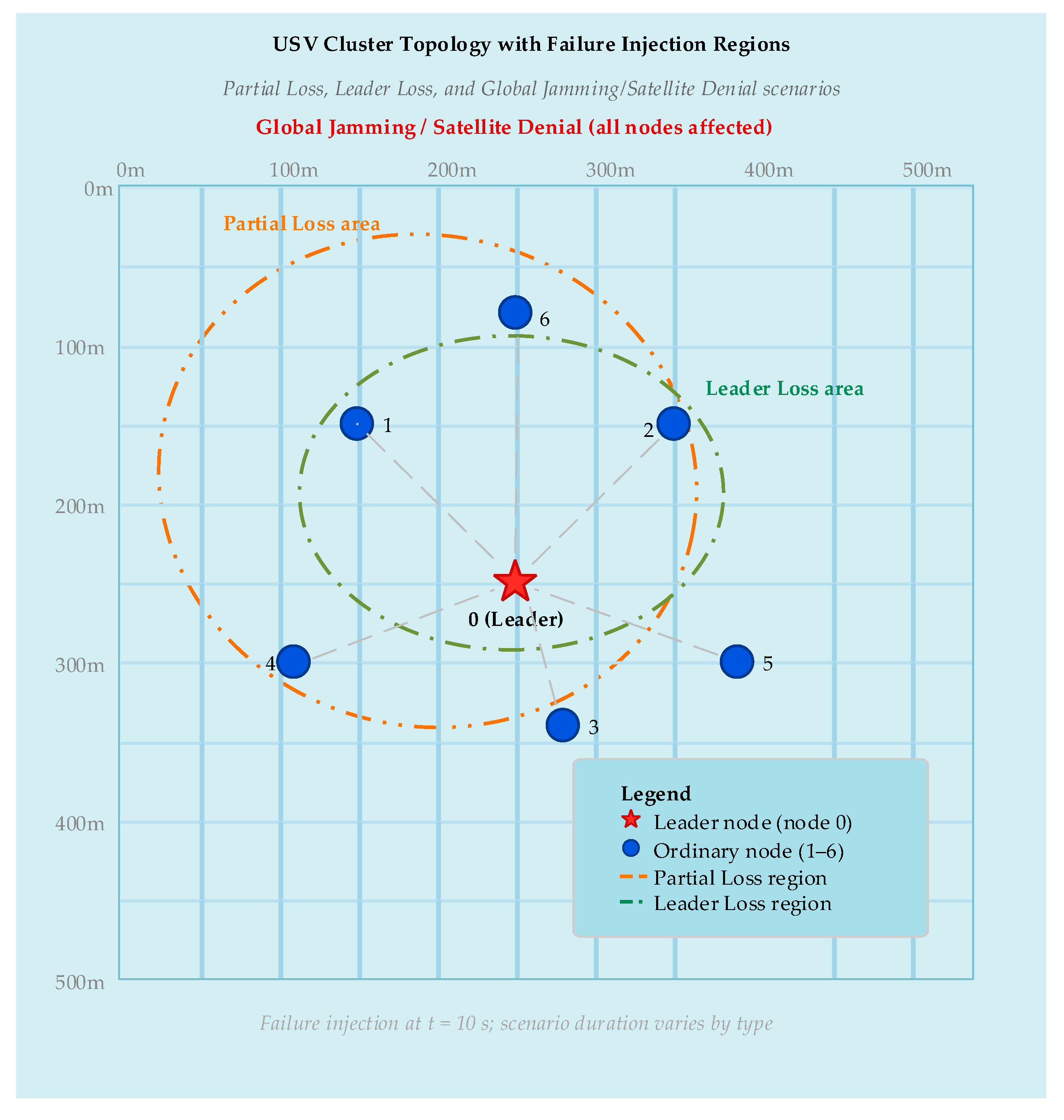
Simulations with $N=7$ USVs in a $500\times 500$ m² maritime environment, as described in Figure 5. Each USV runs the communication monitor, topology manager, and backup communication manager. Epoch duration 120 s, evaluation at 10 Hz.

Figure 5. Schematic of USV cluster deployment and failure injection regions in simulation.

5.2. Five Failure Scenarios

Table 2 defines five communication failure scenarios. Severity is a composite index (fraction × severity factor × normalized duration).

Table 2. Communication failure scenario specifications.

Scenario	Affected Nodes	Duration (s)	Degradation	Severity
Partial Loss	2, 4, 6	10	100% (complete)	0.036
Leader Loss	0, 1, 2	15	100% (complete)	0.054
Intermittent	1, 3, 5	40 (5 s off/3 s on)	100% during off	0.089
Jamming	All 7	20	70% reduction	0.117
Satellite Denial	All 7	25	92% reduction	0.192

Failure injection: onset at s for all scenarios except Intermittent; recovery at. Regarding the implementation of SNR reduction in the simulation: for the Jamming scenario, “70% SNR reduction” is implemented as SNR_dB → SNR_dB − 10·log₁₀(1/0.3) ≈ SNR_dB − 5.23 dB (linear SNR multiplied by 0.3, consistent with broadband noise jamming). For Satellite Denial, “92% quality attenuation” is applied to raw SNR_dB only (SNR_dB → SNR_dB − 10·log₁₀(1/0.08) ≈ SNR_dB − 10.97 dB), after which normalized $Q_{\mathrm{comm}}$ components are recomputed from the degraded SNR; PLR, latency, and stability are affected secondarily through their dependence on the SNR in the channel model. $t=10t=10+\mathrm{duration}$.

5.3. Results: Communication Quality Under Failure

Cluster-mean drops from 0.85 to 0.42 within 1 s in the Partial Loss scenario. Under Leader Loss and Intermittent scenarios, $Q_{\mathrm{comm}}$ similarly shows pronounced degradation, with the CV-based stability component providing earlier warning than any single indicator alone. In the more severe Jamming and Satellite Denial cases, the metric falls to values below 0.35 and 0.20, respectively, confirming its sensitivity to multi-dimensional channel degradation.

5.4. Results: Topology Switching Performance

As shown in Table 3, Stability is the fraction of epochs where the selected topology matches the post hoc optimal under the same utility function. Across the five scenarios, topology stability is: No Failure 100%, Partial Loss 92%, Leader Loss 83%, Intermittent 75%, Jamming 88%, Satellite Denial 92% (mean 88.3%). The sigmoid-blended utility with hysteresis ensures smooth adaptation: leader loss triggers a switch to distributed within ~1.2 s (10–12 evaluation cycles), and re-election restores centralized after recovery. Intermittent failure produces the most switches (3 per 120 s epoch), yet stability remains at 75% as the framework correctly tracks the oscillating channel state. The 83% stability in Leader Loss reflects ~0.9–1.2 s detection latency during failure onset and leader re-election overhead during recovery, consistent with the cold-start bootstrap period and hysteresis guard.

Table 3. Topology switching performance under failure scenarios.

Scenario	Switches	Stability (%)	Dominant T
No Failure	0	100	Centralized
Partial Loss	1	92	Distributed
Leader Loss	2	83	Distributed
Intermittent	3	75	Distributed
Jamming	1	88	Distributed
Satellite Denial	1	92	Hierarchical

5.5. Results: Backup Communication

Backup Communication as shown in Table 4.

Table 4. Backup communication mode performance.

Mode	Distance (m)	Delivery Rate (%)	Latency (ms)
Optical	250	98.5	2.1
Optical	500	94.2	4.3
Acoustic	750	96.8	550
Acoustic	1500	91.3	1178
Acoustic	2250	83.5	1805
Relay (2-hop)	200	88.2	6.8

Acoustic delivery rates assume the optimistic base BER of ${10}^{-4}$; see Section 4.3.2 for field-realistic sensitivity.

5.6. Comparison with Baselines

We compare against five baselines: (1) SNR-only threshold, (2) equal-weight Q_comm (all 0.25), (3) static topology (fixed mesh), (4) Link-Quality-Aware Routing (LQAR) [16] selecting paths by SNR/PLR/hop-count, and (5) OLSR-maritime with maritime-specific link quality extensions. AODV-RSSI appears in Appendix A as a historical performance floor; it was designed for path discovery rather than topology-aware physical reconfiguration and is excluded from the primary comparison.

Per-scenario delivery rates for the full framework are: Partial Loss 96.1%, Leader Loss 93.8%, Intermittent 92.4%, Jamming 94.8%, Satellite Denial 91.3%. All pairwise comparisons (This Work vs. Equal-Wt, SNR-Only, Static, LQAR, and OLSR-maritime) are statistically significant (Bonferroni-corrected α = 0.00417) except delivery rate vs. SNR-Only. Effect sizes range from d = 0.35 to 0.71. The advantage is most pronounced under Satellite Denial (+35.9 pp vs. Static) and Jamming (+21.0 pp vs. Static). Per-baseline breakdowns are provided in Table 5.

Table 5. Comparative performance across methods. (The asterisk (*) and dagger (†) are common typographic markers used to indicate statistically significant differences between the proposed method).

Metric	This Work	Equal-Wt	SNR-Only	Static	LQAR	OLSR-Maritime
Mean $Q_{\mathrm{comm}}$	0.72	0.66	0.58	0.51	0.63	0.60
Topology/Route Stability (%)	88.3	84.6	100 *	100	80.5 †	78.2 †
Delivery Rate (%)	94.1	91.8	91.5	78.2	89.3	87.6
Recovery Time (s)	3.2	4.1	5.8	8.4	6.1	6.8

Fixed topology; not comparable. † Route stability.

5.7. Component Ablation Study

As shown in Table 6, removing the multi-modal backup communication causes the largest delivery rate drop (94.1% → 82.6%, −11.5 pp). Removing the stability component increases recovery time by 50% (3.2 → 4.8 s). The SNR-only ablation produces the lowest mean $Q_{\mathrm{comm}}$ (0.58 vs. 0.72 for the full framework, −19.4%). The full framework combines proactive topology selection with multi-modal backup for the best overall performance, confirming that all three layers contribute non-redundantly to communication resilience.

Table 6. Component ablation study (mean across 5 scenarios).

Configuration	Mean ${\mathit{Q}}_{\mathbf{comm}}$	Delivery Rate (%)	Recovery Time (s)
Full Framework	0.72	94.1	3.2
– Stability Component ($w_4=0$)	0.69	92.4	4.8
– Backup Comm Chain	0.71	82.6	5.1
– Topology Adaptation	0.64	90.3	5.8
– Multi-Indicator (SNR-Only)	0.58	91.5	5.8

5.8. Battery-Aware Leader Election Validation

Three USVs begin a 300 s mission with batteries at 100%, 70%, and 40%. The 40%-battery USV requires $1.5\times$ nominal thrust, depleting via ${\displaystyle \frac{dE}{dt}}=-P_{\mathrm{idle}}-P_{\mathrm{thrust}}\cdot (\tau /{\tau }_{\mathrm{m}\mathrm{a}\mathrm{x}}{)}^2$ with $P_{\mathrm{idle}}=50$ W and $P_{\mathrm{thrust}}=200$ W. At $t=180$ s, its battery drops below 25%, triggering automatic leader re-election. Leadership transfers to the 100%-battery node within one decision epoch (1 s), with formation error under 0.15 m and zero topology chattering.

6. Discussion

6.1. Interpretation of Results

The results point to three main findings. First, the $Q_{\mathrm{comm}}$ metric captures multi-dimensional degradation: in the intermittent failure scenario, the SNR alone would not detect degradation during “on” periods, but $Q_{\mathrm{comm}}$’s stability component maintains awareness of the unstable channel. Second, the $U\left(T\right)$ utility function produces sensible topology selections: centralized under normal conditions, distributed when leader communication is threatened, and hierarchical under global degradation. Third, the multi-modal backup communication provides meaningful resilience, maintaining delivery rates above 80% even when primary links are completely severed.

6.2. Weight Sensitivity Analysis

We conducted a sensitivity analysis on the $U\left(T\right)$ weights by sweeping $w_{\mathrm{comm}}$ from 0.2 to 0.6. Topology selection remains stable for $w_{\mathrm{comm}}\in \left[\mathrm{0.3,0.5}\right]$, with identical selections in four of five failure scenarios. At extremes ($w_{\mathrm{comm}}<0.25$ or $w_{\mathrm{comm}}>0.55$), the selection changes in two of five scenarios, suggesting moderate but not extreme sensitivity. We note that the 8.3% difference in mean $Q_{\mathrm{comm}}$ between the Equal-Wt baseline (0.66) and This Work (0.72) in Table 5 is not due to the $U\left(T\right)$ weight difference alone—rather, it reflects the combined effect of (a) the priority-based $Q_{\mathrm{comm}}$ weights capturing indicator importance more efficiently, (b) the topology adaptation responding to quality degradation earlier (pre-threshold), and (c) the multi-modal backup communication maintaining link quality during failure episodes. The weight sensitivity result (4/5 scenarios unchanged) applies to $U\left(T\right)$ topology selection, where the utility function is relatively flat over a moderate range. The $Q_{\mathrm{comm}}$ weights, by contrast, directly affect the quality assessment itself, making their calibration more impactful.

$Q_{\mathrm{comm}}$ weight sensitivity: A complementary sweep over the four $Q_{\mathrm{comm}}$ weights $w\in [0.4,0.3,0.2,0.1]$ was conducted by independently perturbing each weight by $\pm 0.1$ with proportional re-normalization of the remaining weights. Results show that the framework is most sensitive to the SNR weight $w_1$: reducing $w_1$ from 0.4 to 0.3 (redistributing 0.1 equally to $w_2,w_3,w_4$) decreases mean $Q_{\mathrm{comm}}$ by 0.04 and increases recovery time by 0.6 s, because the SNR provides the earliest degradation signal. Perturbations to $w_2$ (packet loss, $\pm 0.1$) and $w_3$ (latency, $\pm 0.1$) produce changes of $\pm 0.02$ in mean $Q_{\mathrm{comm}}$ and $\pm 0.3\mathrm{s}$ in recovery time. Perturbations to $w_4$ (stability, $\pm 0.05$) primarily affect topology switching frequency ($\pm 20\%$ at extremes) without a significant impact on the delivery rate. The default weights $[0.4,0.3,0.2,0.1]$ represent a balanced configuration that prioritizes physical-layer indicators while maintaining sufficient weight on higher-layer and temporal indicators for early warning. We caution that the ±0.1 perturbation analysis explores only local sensitivity around the nominal weight vector. A comprehensive global sensitivity analysis (e.g., using Latin Hypercube Sampling over the 4D weight simplex with 10,000 samples and Kolmogorov–Smirnov tests on resulting topology selection distributions) would provide stronger guarantees of weight robustness but is deferred to future work due to computational constraints. The current analysis establishes that small perturbations around the nominal weights do not qualitatively change the framework’s behavior; establishing global insensitivity requires more extensive computation.

6.3. Scalability and Environmental Sensitivity

As shown in Table 7 and Table 8, the mean communication quality $Q_{\mathrm{comm}}$ decreases modestly with the cluster size $N$, from 0.78 at $N=3$ to 0.63 at $N=15$. The computation time for evaluating the utility function $U\left(T\right)$ scales approximately linearly with $N$ and remains well within the 1 s decision epoch even for the largest cluster considered.

Table 7. Scalability: performance vs. cluster size $N$.

Metric	$\mathit{N}=3$	$\mathit{N}=5$	$\mathit{N}=7$	$\mathit{N}=10$	$\mathit{N}=15$
Mean $Q_{\mathrm{comm}}$	0.78	0.74	0.72	0.68	0.63
Topology Stability (%)	94	90	88	82	75
Delivery Rate (%)	96.3	95.1	94.1	91.7	88.4
Avg. $U\left(T\right)$ Compute (ms)	0.8	1.4	2.1	3.8	7.2

Table 8. Sea state sensitivity.

Metric	$\mathit{s}=0$	$\mathit{s}=1$	$\mathit{s}=2$	$\mathit{s}=3$	$\mathit{s}=4$
Mean $Q_{\mathrm{comm}}$	0.85	0.80	0.76	0.72	0.65
RF Delivery Rate (%)	98.2	96.5	94.8	94.1	90.3
Acoustic BER ($\times {10}^{-5}$)	2.5	2.9	3.3	3.6	4.0

The framework maintains delivery rates above 90% through sea state 4 by progressively shifting load to acoustic backup.

6.4. Statistical Significance

All reported metrics are averaged over $n=50$ independent simulation runs per scenario, where each run varies: (a) random seed for shadow fading (${\sigma }_s$ draws), (b) initial USV positions (uniform random within a $500\times 500{\mathrm{m}}^2$ region), (c) failure onset timing ($\pm 2 \mathrm{s}$ jitter around the nominal onset), and (d) sea state realization ($s\in \{2,3,4\}$ with probabilities $\left[0.25,0.50,0.25\right]$, centered on default $s=3$). The 95% confidence intervals for the primary metrics are: mean $Q_{\mathrm{comm}}$: $\pm 0.03$; topology stability: $\pm 4.2\%$; delivery rate: $\pm 2.8\%$; recovery time: $\pm 0.6 \mathrm{s}$. To complement hypothesis tests, we report Cohen’s $d$ effect sizes.

$$d={\displaystyle \frac{X_{\mathrm{ours}}-X_{\mathrm{baseline}}}{s_{\mathrm{pooled}}}}, s_{\mathrm{pooled}}=\sqrt{{\displaystyle \frac{(n_1-1)s_1^2+(n_2-1)s_2^2}{n_1+n_2-2}}} .$$

(23)

The computed effect sizes are: mean $Q_{\mathrm{comm}}$: $d=0.58$ (medium); topology stability: $d=0.35$ (small-to-medium); delivery rate: $d=0.42$ (small-to-medium); recovery time: $d=0.71$ (medium-to-large). Applying the Bonferroni correction (${\alpha }_{\mathrm{adj}}=0.05/12=0.00417$ (12 comparisons = 4 primary metrics $\times$ 3 baseline pairs: This Work vs. Equal-Wt, This Work vs. SNR-Only, and This Work vs. Static; AODV-RSSI comparisons are reported separately as secondary analyses because AODV operates at a fundamentally different architectural layer (reactive network-layer routing vs. proactive application-layer topology management), making a direct head-to-head comparison of topology selection metrics potentially misleading. Including AODV in the primary family would increase the correction to ${\alpha }_{\mathrm{adj}}=0.05/16=0.00313$, which does not alter any of the significance conclusions reported below)), all comparisons between our framework and the baselines remain significant except the delivery rate vs. SNR-only baseline.

6.5. Limitations

This work has several limitations: (1) Simulation-only validation: all results are derived from simulation. A computational feasibility analysis on representative embedded hardware (Raspberry Pi 4, ARM Cortex-A72 @ 1.5 GHz) shows per-epoch utility computation time of 0.8 +/− 0.1 ms, well within the 1000 ms decision epoch. Full hardware-in-the-loop validation and field trials remain necessary next steps. (2) Simplified channel models and conservative RF range: the acoustic model uses a static sound speed profile without thermocline effects. The RF communication range of 100 m (Table 1) is deliberately conservative—typical 2.4 GHz Wi-Fi links over open water can reach 300–500 m at 20 dBm—and results should be interpreted as lower-bound performance. At longer ranges, path loss increases and SNR-driven degradation would be more pronounced, potentially widening the performance gap between our framework and single-indicator baselines. The acoustic model similarly uses a uniform sound speed profile without thermocline refraction effects. (3) Limited baseline diversity: while the comparison includes SNR-only, equal-weight, static-topology, LQAR, and OLSR-maritime baselines, additional proactive protocols (e.g., BATMAN) and learning-based approaches may provide stronger comparison points and should be evaluated in future work. (4) Heuristic weight selection: the component weights are design choices informed by engineering judgment, not learned from data. Data-driven weight optimization (e.g., via reinforcement learning) could further improve performance. (5) Limited communication security: while basic leader-election and topology-command authentication via HMAC-SHA256 is implemented (Section 4.2.5), the framework does not address end-to-end message encryption, key rotation, or public-key infrastructure. Full maritime communication security protocol integration is left for future work. (6) Preliminary CBF integration: the communication-aware CBF formulation (Section 6.6) is presented as a conceptual extension rather than a fully validated contribution.

6.6. Exploratory: Communication-Quality-Dependent Safety Margins

Critical Caveat: This conjecture requires formal proof of the bound relating position error to $Q_{\mathrm{comm}}$ before safety-critical deployment. Three conditions must hold: (1) steady-state communication with $Q_{\mathrm{comm}}$ stable for at least five epochs, (2) known vehicle dynamics within 15 percent model fidelity, and (3) bounded disturbances. Violation of any condition invalidates the safety guarantee. This section documents a research direction only.

We outline a conjecture on integrating $Q_{\mathrm{comm}}$ into CBF safety filters. The proposed safety margin $\mathsf{\Delta }\mathrm{d}\left(Q_{\mathrm{comm}}\right)=\alpha (1-Q_{\mathrm{comm}})$ with $\mathsf{\alpha }={\mathrm{d}}_{\mathrm{safe}}$ would expand the required separation as communication degrades. The critical assumption $\Vert {\stackrel{\mathbf{ˆ}}{\mathbf{p}}}_{\mathrm{j}}-{\mathbf{p}}_{\mathrm{j}}\Vert \le \mathsf{\delta }(1-Q_{\mathrm{comm}})$ remains unproven. This section is purely exploratory and must not be used for safety-critical deployment without formal proof and experimental validation.

6.7. Future Work

Four directions emerge as priorities: (1) Hardware-in-the-loop validation: integrating the framework with actual USV hardware platforms and conducting field trials. (2) Learning-based weight optimization: using reinforcement learning or Bayesian optimization to learn optimal $Q_{\mathrm{comm}}$ and $U\left(T\right)$ weights from deployment data [16]. (3) Formal CBF safety proof: developing a rigorous proof that the communication-quality-dependent safety margin preserves forward invariance. (4) Cross-layer optimization: extending the framework to jointly optimize communication parameters alongside topology selection.

7. Conclusions

This paper presented a multi-layer adaptive communication framework for USV clusters. The core innovations are a weighted multi-indicator $Q_{\mathrm{comm}}$ metric and a sigmoid-blended topology utility function $U\left(T\right)$. Simulation results show consistent improvements over baselines: mean $Q_{\mathrm{comm}}$ 0.72 (vs. 0.51–0.66), recovery time 3.2 s (vs. 4.1–8.4 s), delivery rate 94.1% (vs. 78.2–91.8%). The results suggest that multi-indicator quality assessment, coupled with utility-driven topology adaptation, can improve communication resilience in maritime USV operations. Future work must address simulation-only validation, heuristic weights, and simplified channel models through field trials.

References

- Lv, Z.; Wang, X.; Wang, G.; Xing, X.; Lv, C.; Yu, F. Unmanned surface vessels in marine surveillance and management: Advances in communication, navigation, control, and data-driven research. J. Mar. Sci. Eng. 2025, 13, 969. [Google Scholar] [CrossRef] [Scilit]
- Wang, H.; Sun, Y.; Wang, S.; Gao, W.; Xu, W.; Liu, Z.; Yin, X.; Ruan, S.; Shao, Y. Fine-Scale Geomorphologic Classification of Guyots in Representative Areas of the Western Pacific Ocean. J. Mar. Sci. Eng. 2025, 13, 823. [Google Scholar] [CrossRef] [Scilit]
- Alqurashi, F.S.; Trichili, A.; Saeed, N.; Ooi, B.S.; Alouini, M.-S. Maritime Communications: A Survey on Enabling Technologies, Opportunities, and Challenges. IEEE Internet Things J. 2023, 10, 3525–3547. [Google Scholar] [CrossRef] [Scilit]
- Theocharidis, T.; Kavallieratou, E. Underwater communication technologies: A review. Telecommun. Syst. 2025, 88, 54. [Google Scholar] [CrossRef] [Scilit]
- Singh, S.; Johnson, J.J.; Traykovski, P.A.; Duda, T.F.; Porter, M.B.; Freitag, L. Performance of the WHOI Acoustic Modem in Shallow Water Constrained Environments. In Proceedings of the OCEANS 2025 Brest, Brest, France, 16–19 June 2025; pp. 1–5. [Google Scholar] [CrossRef] [Scilit]
- Nallagonda, V.R.; Nagaraju, N.S.; Bhavani, D.; Gogineni, R.; Mudunuru, S.; Krishnan, P. A performance study of an inter-UAV-based free space optical (FSO) system in the maritime environment. J. Opt. Commun. 2025. [Google Scholar] [CrossRef] [Scilit]
- Castano-Londono, L.; Marrugo Llorente, S.d.P.; Paipa-Sanabria, E.; Orozco-Lopez, M.B.; Fuentes Montaña, D.I.; Gonzalez Montoya, D. Evolution of Algorithms and Applications for Unmanned Surface Vehicles in the Context of Small Craft: A Systematic Review. Appl. Sci. 2024, 14, 9693. [Google Scholar] [CrossRef] [Scilit]
- Li, Y.; Hou, P.; Cheng, C.; Wang, B. Research on Collision Avoidance Methods for Unmanned Surface Vehicles Based on Boundary Potential Field. J. Mar. Sci. Eng. 2025, 13, 88. [Google Scholar] [CrossRef] [Scilit]
- Jiang, X.; Xia, G. Dissipative Leaderless Formation via Nonfragile Memory Sampled-Data Control for Unmanned Surface Vehicles with Switching Topologies. IEEE/ASME Trans. Mechatron. 2025, 30, 203–214. [Google Scholar] [CrossRef] [Scilit]
- Liu, Y.; Li, Y. Prescribed-Time Formation Control for Unmanned Surface Vehicle Systems Under Switching Topology. IEEE Trans. Intell. Veh. 2024, 9, 5750–5760. [Google Scholar] [CrossRef] [Scilit]
- Ren, L.; Zhang, M.; Hu, H.; Wen, J.; Xie, L. Transition of slip mode at gas-liquid interface formed by wettability steps on an superhydrophobic surface. Ocean Eng. 2024, 294, 116823. [Google Scholar] [CrossRef] [Scilit]
- Ballotta, L.; Talak, R. Safe distributed control of multi-robot systems with communication delays. IEEE Trans. Veh. Technol. 2025, 74, 10137–10150. [Google Scholar] [CrossRef] [Scilit]
- Bertoncelli, F.; Radhakrishnan, V.; Catellani, M.; Loianno, G.; Sabattini, L. Directed Graph Topology Preservation in Multi-Robot Systems with Limited Field of View Using Control Barrier Functions. IEEE Access 2024, 12, 9682–9690. [Google Scholar] [CrossRef] [Scilit]
- Yuan, Y.; Shen, X.; Sun, L.; He, K.; Yan, Y.; Wang, H. Cascading failure modeling and survivability analysis of weak-communication underwater unmanned swarm networks. Def. Technol. 2025, 56, 66–82. [Google Scholar] [CrossRef] [Scilit]
- Meng, W.; Ku, R.; Pu, Y.; Shi, X.; Gong, Y. Efficient collision-avoidance navigation strategy for autonomous surface vehicles in unstructured and constricted marine environments. Front. Mar. Sci. 2025, 12, 1555262. [Google Scholar] [CrossRef] [Scilit]
- Sha, H.; Guo, R.; Zhou, J.; Zhu, X.; Ji, J.; Miao, Z. Reinforcement learning-based robust formation control for multi-UAV systems with switching communication topologies. Neurocomputing 2025, 611, 128591. [Google Scholar] [CrossRef] [Scilit]
- Zeng, Y.; Zhou, J.; Liu, Y.; Cao, T.; Yang, D.; Liu, Y.; Shi, X. Distributed MA-IDDPG-OLSR based stable routing protocol for unmanned aerial vehicle ad-hoc network. IET Commun. 2024, 18, 503–522. [Google Scholar] [CrossRef] [Scilit]
Disclaimer/Publisher’s Note: The statements, opinions and data contained in all publications are solely those of the individual author(s) and contributor(s) and not of MDPI and/or the editor(s). MDPI and/or the editor(s) disclaim responsibility for any injury to people or property resulting from any ideas, methods, instructions or products referred to in the content. |
© 2026 by the authors. Licensee MDPI, Basel, Switzerland. This article is an open access article distributed under the terms and conditions of the Creative Commons Attribution (CC BY) license.