Existence of Crossing Periodic Solutions of a Duffing Equation with Discontinuity

Abstract

Classical periodic solution theories of undamped Duffing equations are mostly restricted to continuous nonlinearities, while discontinuous models from mechanical impact and switching circuits lack systematic existence criteria for crossing periodic orbits. This work addresses a second-order undamped Duffing system with jump discontinuity of $g\left(x\right)$ on $x=0$, where $g\left(x\right)$ is piecewise continuously differentiable on two half real axes. With the separation condition ruling out sliding trajectories on the discontinuity line, the continuity of the Poincaré map is proved by Filippov theory for discontinuous ODEs. Using the Poincaré–Bohl fixed-point theorem, we derive multiple sufficient conditions ensuring the existence of $2\pi$ crossing periodic solutions via successive relaxation of growth hypotheses, and a numerical test example confirms the practicability of our theoretical findings, extending classical continuous Duffing results to discontinuous dynamical systems.

1. Introduction

The periodic solution problem for the undamped second-order Duffing equation

$$\ddot{x}+g\left(x\right)=p\left(t\right)$$

(1)

serves as a cornerstone in the fields of nonlinear oscillation theory and qualitative analysis of differential equations. This is primarily because, despite its seemingly simple form, the research approaches and core ideas developed for this equation provide crucial theoretical references and methodological guidance for investigating more complex nonlinear differential equations, which are widely encountered in physics, engineering, and other applied disciplines.

It is well-documented that extensive and in-depth research has been conducted on the periodic solutions of Equation (1) over the past decades. Specifically, when $g:\mathbb{R}\to \mathbb{R}$ is a continuous function and $p:\mathbb{R}\to \mathbb{R}$ is continuous and T-periodic, a series of classical existence, nonexistence, and multiplicity results have been established. These conclusions are typically derived under the assumption that the nonlinear term g satisfies certain growth conditions, such as superlinearity, sublinearity, and semilinearity. In [1], Ding et al. investigated the periodic solution problem of Equation (1) under the semilinear growth condition

$$0<g_{*}:=\underset{\left|x\right|\to +\infty }{lim\; inf}{\displaystyle \frac{g\left(x\right)}{x}}\le \underset{\left|x\right|\to +\infty }{lim\; sup}{\displaystyle \frac{g\left(x\right)}{x}}:=g^{*}<+\infty$$

and obtained comprehensive results concerning the existence, nonexistence, and multiplicity of harmonic and subharmonic solutions. Additionally, in [2], Ding and Zanolin studied the periodic solutions of Equation (1) where the nonlinearity g satisfies the sublinear condition

$$\underset{\left|x\right|\to \infty }{lim}{\displaystyle \frac{g\left(x\right)}{x}}=0.$$

For periodic solutions of Equation (1) under superlinear growth conditions, interested readers may refer to [3] for detailed results. In [4], Wang further extended the research by considering the existence of periodic solutions for Equation (1) where the nonlinear term g satisfies an asymmetric growth condition

$$q_1\le {\displaystyle \frac{g\left(x\right)}{x}}\le p_1,x\le -A_1;q_2\le {\displaystyle \frac{g\left(x\right)}{x}},x\ge A_1,$$

where $q_1,q_2,p_1,A_1$ are positive constants. Meanwhile, the applications of planar analysis, time-map methods, and degree theory in solving such periodic solution problems have been fully demonstrated in [5,6,7], laying a solid methodological foundation for subsequent research.

In recent years, with the rapid development of research on discontinuous differential equations [8,9,10,11], exploring the qualitative properties and periodic solutions of discontinuous Duffing equations has become an inevitable and promising research trend. This is due to the fact that discontinuous nonlinearities are frequently observed in practical engineering systems, such as mechanical oscillators with impact, electrical circuits with switching, and elastic structures with piecewise stiffness. From the perspective of engineering realization, Chawla et al. constructed an analog electronic circuit to verify the dynamic characteristics of Filippov-type discontinuous impact oscillators and proposed a high-precision higher-order discontinuity mapping method for discontinuous boundary dynamics analysis [12], while Wang et al. uncovered complicated bursting oscillation mechanisms induced by multiple crossing bifurcations inherent to piecewise-smooth nonlinear systems [13], both of which provide typical engineering prototypes for the mathematical modeling of discontinuous Duffing-type models.

In [14], Chen and Xie studied an oscillating model of elastic beams described by

$$x^{″}+x\left(1-{\displaystyle \frac{1}{\sqrt{a^2+x^2}}}\right)=e\left(t\right),$$

where discontinuous dynamic behavior arises when $a=0$. In [15], Chen et al. further investigated the existence and multiplicity of harmonic and subharmonic solutions for a class of damped second-order Duffing equations with $g\left(x\right)=x+sgn\left(x\right)$, which exhibits discontinuous characteristics. In [16], Jiang et al. investigated discontinuous damped Duffing equations with a discontinuous restoring force, established the geometric properties of solutions, and applied the Poincaré–Bohl theorem to prove the existence and uniqueness of crossing harmonic and subharmonic periodic solutions. In [17], Jiang further considered undamped discontinuous Duffing systems with vector-field discontinuity at the origin, and employed the generalized Poincaré–Birkhoff theorem to verify the existence of infinitely many large-amplitude periodic solutions. In [18], Jiang extended the research scope to discontinuous mixed-type Duffing equations with asymmetric nonlinear growth conditions, and presented multiple existence criteria together with a uniqueness conclusion for crossing periodic solutions. Notably, all three studies treated the nonlinear term g as an abstract general function rather than a specific expression, which significantly improves the universality and applicability of the theoretical results.

Notably, classical fixed point theorems and Filippov theory [19] play an irreplaceable role in solving periodic solution problems of discontinuous Duffing equations, providing effective tools for handling discontinuities. Guo and Luo systematically analyzed the generation mechanism and classification of periodic motion bifurcations governed by Filippov discontinuous dynamical systems [20], and Lai and Chen clarified the numerical computation pitfalls of Floquet multipliers caused by system piecewise-smooth boundaries, correcting the miscalculation of stability indicators near discontinuity interfaces [21]. In addition, Niu and Li considered the existence of periodic solutions for semilinear Duffing equations with impulsive effects in [22], expanding the research scope to impulsive–discontinuous hybrid systems. Moreover, Jiang studied the existence and uniqueness of discontinuous periodic orbits in second order differential equations with state-dependent impulses [23], which further enriches the research on discontinuous periodic solutions. In parallel theoretical progress, Nieto and Uzal discussed subharmonic periodic solutions of state-dependent discontinuous differential equations under superlinear and sublinear growth restrictions [10], and Wen et al. gave rigorous existence and uniqueness judgments for periodic solutions of second-order impulsive discontinuous differential systems [11]. In [24], Freire et al. established a canonical form for planar discontinuous piecewise linear Filippov systems and systematically analyzed limit cycle bifurcations around the sliding set. In [25], Zhou et al. investigated harmonic solutions of non-autonomous piecewise linear oscillators by distinguishing resonant and non-resonant cases and presented corresponding existence and uniqueness criteria. Furthermore, Jia et al. addressed the global phase portraits and bifurcation behaviors of three-zone continuous piecewise linear systems in [26], revealing complex dynamical phenomena such as homoclinic loops and multiple limit cycles. These theoretical results on piecewise smooth dynamical systems also offer valuable insights into the local dynamic behavior of Equation (1) near discontinuity points.

Despite the aforementioned progress, there remain unresolved issues in the study of periodic solutions for discontinuous undamped Duffing equations, particularly regarding the influence of discontinuity lines on the existence and multiplicity of periodic solutions. Motivated by these research gaps, this paper focuses on the periodic solution problem of Equation (1) with a discontinuity line, aiming to establish new existence criteria and enrich the existing theoretical system.

This paper is organized as follows: In Section 2, we present some necessary preliminaries related to the undamped second-order Duffing equation with a discontinuity line, including basic definitions, lemmas, and relevant theoretical tools. In Section 3, we prove several key lemmas and establish the main existence results of $2\pi$ crossing periodic solutions by virtue of the Poincaré–Bohl theorem (Theorem 1) and gradually relax the restrictive assumptions to generalize the obtained conclusions for wider applicability. In Section 4, a concrete numerical example with phase-plane simulation is presented to verify the feasibility, computability and effectiveness of the derived theoretical criteria. In Section 5, we discuss the core innovations, theoretical extensions, research limitations and academic contributions of this work, and elaborate the differences and connections between the proposed results and classical continuous Duffing theories. Finally, we summarize the full research content of the paper and propose detailed future research directions in Section 6.

2. Preliminaries

In this paper, we assume that ${\Sigma }_0=\{(x,y)\in {\mathbb{R}}^2:x=0\}$ divides the function $g\left(x\right)$ into the following form:

$$g\left(x\right)=\left\{\begin{array}{cc}{g}_{+}\left(x\right),\hfill & x>0,\hfill \\ g_{-}\left(x\right),\hfill & x<0.\hfill \end{array}\right.$$

And we consider the discontinuous second-order undamped Duffing equation of the form

$$\ddot{x}+g_{\pm }\left(x\right)=p\left(t\right),x\ne 0,$$

(2)

where $g_{+}\left(x\right)\in C^1([0,+\infty ),\mathbb{R})$, $g_{-}\left(x\right)\in C^1((-\infty ,0],\mathbb{R})$, and $p:\mathbb{R}\to \mathbb{R}$ is continuous and $2\pi$-periodic. We define

$$\underline{\beta }=\underset{t\in [0,2\pi ]}{min}p\left(t\right),\overline{\beta }=\underset{t\in [0,2\pi ]}{max}p\left(t\right),\beta =\underset{t\in [0,2\pi ]}{max}\left|p\left(t\right)\right|.$$

(3)

Here ${\Sigma }_0$ is called a discontinuity line on the plane, which partitions the plane into the left-hand and right-hand half-planes, and we denote as

$$\begin{array}{c}\hfill {\Sigma }_0^{-}=\{(x,y)\in {\mathbb{R}}^2:x<0\},{\Sigma }_0^{+}=\{(x,y)\in {\mathbb{R}}^2:x>0\},\end{array}$$

then ${\mathbb{R}}^2={\Sigma }_0^{-}\cup {\Sigma }_0\cup {\Sigma }_0^{+}$, and the unit normal vector to ${\Sigma }_0$ is $\mathit{n}={(1,0)}^T$.

The Duffing Equation (2) can also be rewritten in the following equivalent form:

$$\left\{\begin{array}{c}\dot{x}=y,\hfill \\ \dot{y}=-g_{\pm }\left(x\right)+p\left(t\right),x\ne 0.\hfill \end{array}\right.$$

(4)

We first impose the following condition on Equation (2).

($G_1$)

The behavior of $g_{\pm }$ at $x=0$ satisfies that the left and right limits exist,

$$\underset{x\to 0^{-}}{lim}{g}_{-}\left(x\right)=g_{-}\left(0\right),\underset{x\to 0^{+}}{lim}{g}_{+}\left(x\right)=g_{+}\left(0\right)$$

and $g_{-}\left(0\right)\ne g_{+}\left(0\right).$

Definition 1.

[Transverse Intersection] Let $\mathit{n}$ be the unit normal vector to the discontinuity line ${\Sigma }_0$. A trajectory of the discontinuous system intersects ${\Sigma }_0$ transversely at a point $(0,y)\in {\Sigma }_0$ if the normal components of the vector fields ${\mathit{f}}_{-}$ and ${\mathit{f}}_{+}$ satisfy

$$\left({\mathit{n}}^{\top }{\mathit{f}}_{-}\right)\left({\mathit{n}}^{\top }{\mathit{f}}_{+}\right)>0.$$

Then the point $(0,y)$ is called as a crossing point. Otherwise, sliding motion may occur. The set of all sliding points is called as a sliding set.

By $\left(G_1\right)$, the solutions of the equation on ${\Sigma }_0$ admit only the origin $O(0,0)$ as a possible sliding point, with transverse intersections occurring everywhere else. In fact, for any $(0,y)\in {\Sigma }_0$ we denote by

$${\mathit{f}}_{-}(0,y)={\left(y,-g_{-}\left(0\right)+p\left(t\right)\right)}^T,{\mathit{f}}_{+}(0,y)={\left(y,-g_{+}\left(0\right)+p\left(t\right)\right)}^T,$$

it follows that

$$\left({\mathit{n}}^{\top }{\mathit{f}}_{-}\right)\left({\mathit{n}}^{\top }{\mathit{f}}_{+}\right)=y^2\ge 0.$$

This means that the origin $O(0,0)$ is the unique possible sliding point on ${\Sigma }_0$. Therefore, in the paper we study the existence of crossing periodic solutions. Here a crossing periodic solution is defined as a periodic solution which does not share points with a sliding set.

Now we recall an existence result of periodic solutions from the Poincaré–Bohl theorem. Here $B_{r_0}$ denotes the closed disk centered at the origin with radius $r_0>0$,

$$B_{r_0}=\left\{(x,y)\in {\mathbb{R}}^2|\sqrt{x^2+y^2}\le r_0\right\}$$

and $S_{r_0}$ denotes the circle bounding $B_{r_0}$, namely the boundary of $B_{r_0}$,

$$S_{r_0}=\partial B_{r_0}=\left\{(x,y)\in {\mathbb{R}}^2|\sqrt{x^2+y^2}=r_0\right\}.$$

Theorem 1.

If a continuous mapping $f:B_{r_0}\to {\mathbb{R}}^2:(\xi ,\eta )\mapsto (u,v)$ satisfies the boundary condition

$$(u,v)\ne \lambda (\xi ,\eta )$$

for any $\lambda \ge 1$ and $(\xi ,\eta )\in S_{r_0}$, then f has at least one fixed point in $B_{r_0}$.

To apply Theorem 1 to establish the existence of $2\pi$ crossing periodic solutions of (2), we first need to ensure that the Poincaré map is well-defined and continuous. Hence we introduce the following condition.

(G₂)

When $g_{-}\left(0\right)<g_{+}\left(0\right)$, there holds

$$[g_{-}\left(0\right),g_{+}\left(0\right)]\cap [\underline{\beta },\overline{\beta }]=\varnothing ;$$

while for $g_{-}\left(0\right)>g_{+}\left(0\right)$ then

$$[g_{+}\left(0\right),g_{-}\left(0\right)]\cap [\underline{\beta },\overline{\beta }]=\varnothing ,$$

where $\underline{\beta }$ and $\overline{\beta }$ come from (3).

Up to now, the existence and uniqueness of solutions to the initial value problem associated with (2) are guaranteed only for initial points located in ${\Sigma }_0^{-}$ or ${\Sigma }_0^{+}$, before the solution trajectories intersect the discontinuity line. This conclusion follows directly from the Picard–Lindelöf theorem [27]. Specifically, $g_{+}\in C^1([0,+\infty ),\mathbb{R})$ and $g_{-}\in C^1((-\infty ,0],\mathbb{R})$, and the mapping $p:\mathbb{R}\to \mathbb{R}$ is continuous. Nevertheless, the global existence and uniqueness of solutions over the entire plane will be rigorously verified after establishing Lemma 1.

For subsequent analysis, let $x\left(t\right)=x(t;x_0,y_0)$ and $y\left(t\right)=y(t;x_0,y_0)$ denote the solution to system (4) with the given initial value $x\left(0\right)=x_0$ and $y\left(0\right)=y_0$. We further use $P(x_0,y_0;0,2\pi )$ to represent the orbit of the solution $(x(t;x_0,y_0),y(t;x_0,y_0))$ for $t\in [0,2\pi ]$. In the sequel, we proceed to prove the continuity of the Poincaré map for system (4).

Lemma 1.

Let $\left(G_1\right)$–$\left(G_2\right)$ hold, then the Poincaré map of the system (4)

$$f:{\mathbb{R}}^2\to {\mathbb{R}}^2,(x_0,y_0)\mapsto (u,v)$$

exists and is continuous, where $u=x(2\pi ;x_0,y_0)$ and $v=y(2\pi ;x_0,y_0)$.

Proof. 

By $\left(G_2\right)$, the situations to be considered are listed below:

$$\left(C_1\right):g_{-}\left(0\right)<g_{+}\left(0\right)<\underline{\beta }<\overline{\beta },\left(C_2\right):g_{+}\left(0\right)<g_{-}\left(0\right)<\underline{\beta }<\overline{\beta },$$

$$\left(C_3\right):\underline{\beta }<\overline{\beta }<g_{-}\left(0\right)<g_{+}\left(0\right),\left(C_4\right):\underline{\beta }<\overline{\beta }<g_{+}\left(0\right)<g_{-}\left(0\right).$$

Here, we take the situation

$$\left(C_1\right):g_{-}\left(0\right)<g_{+}\left(0\right)<\underline{\beta }<\overline{\beta }$$

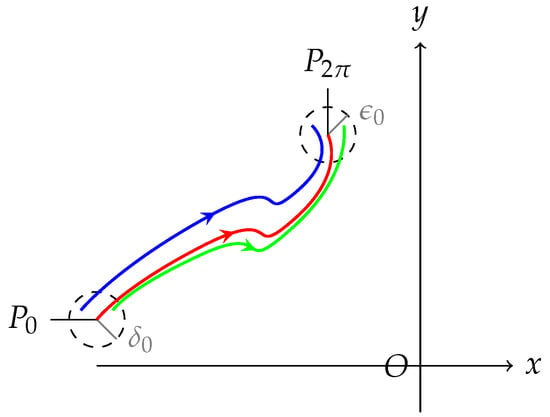
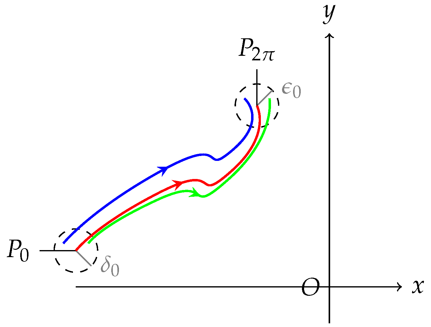
as an example. The remaining cases are similar and therefore omitted. Let $P_t\in P(x_0,y_0;0,2\pi )$ denote the position of the orbit at time t ($\in [0,2\pi ]$). If the orbit lies entirely in ${\Sigma }_0^{+}$ or ${\Sigma }_0^{-}$, then $P(x_0,y_0;0,2\pi )$ exists uniquely. By using the theorem of continuous dependence of solutions on initial conditions, we can conclude that f is continuous, as shown in Figure 1.

Next, we will focus on the points of $P(x_0,y_0;0,2\pi )$ in ${\Sigma }_0$. Let ${\Sigma }_{0^{+}}=\{(x,y)\in {\mathbb{R}}^2\mid x=0,y>0\}$ and ${\Sigma }_{0^{-}}=\{(x,y)\in {\mathbb{R}}^2\mid x=0,y<0\}$.

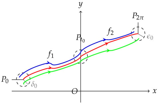
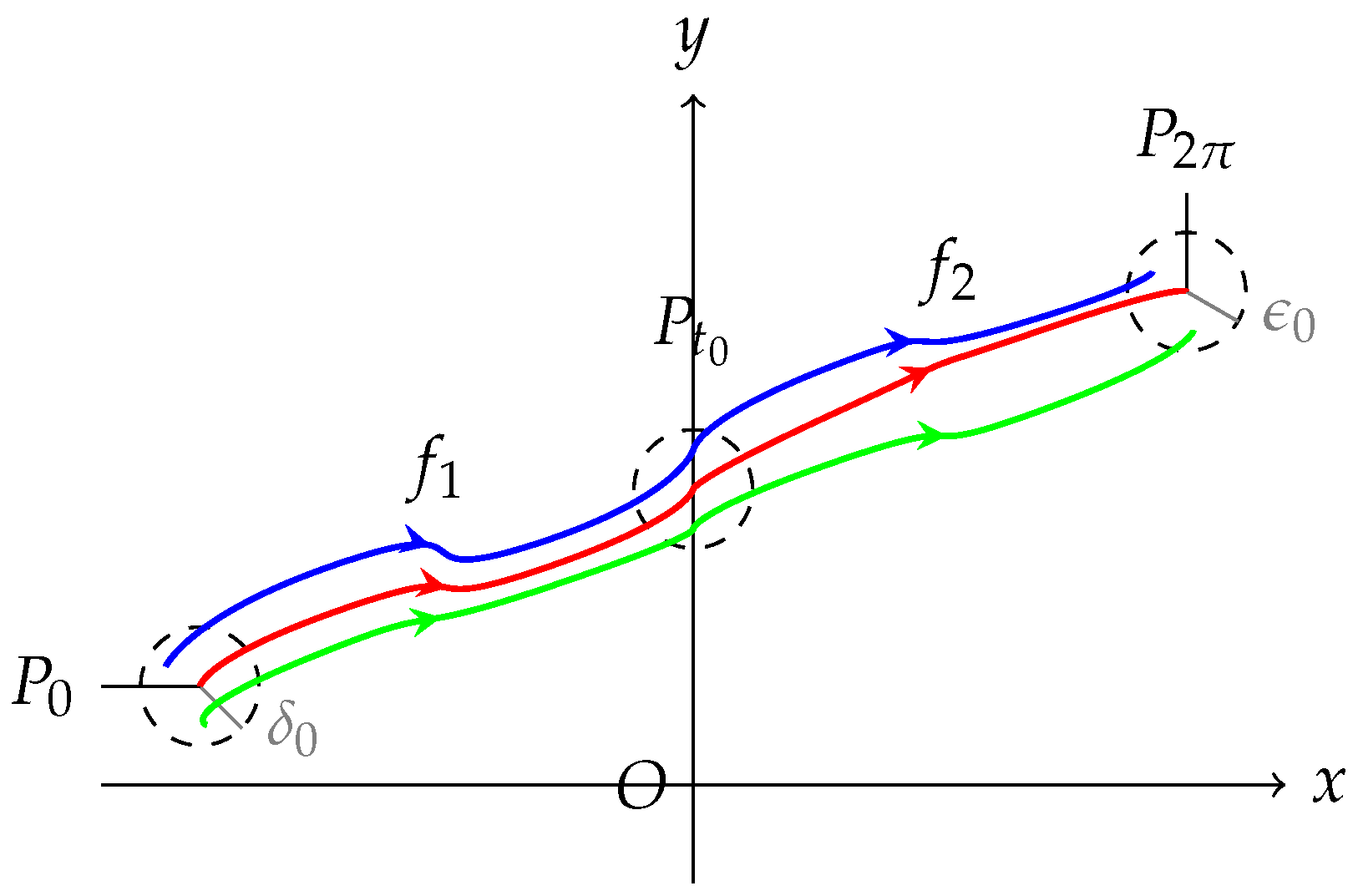
We first suppose that there exists $t_0\in [0,2\pi ]$ such that $P_{t_0}\in {\Sigma }_{0^{+}}\cup {\Sigma }_{0^{-}}$ and $O\notin P(x_0,y_0;0,2\pi )$. Taking $P_{t_0}\in {\Sigma }_{0^{+}}$ as an example, and the case for $P_{t_0}\in {\Sigma }_{0^{-}}$ is similar. Since the Equation (2) satisfies the transversal intersection condition on ${\Sigma }_{0^{+}}$, we can guarantee the existence of the mapping f. In order to verify the continuity of f, we should divide f into left and right Poincaré maps $f_1$ and $f_2$ where $f_1:{\Sigma }_0^{-}\to {\Sigma }_{0^{+}}$ and $f_2:{\Sigma }_{0^{+}}\to {\Sigma }_0^{+}$. So $f=f_1\circ f_2$ is continuous, as shown in Figure 2.

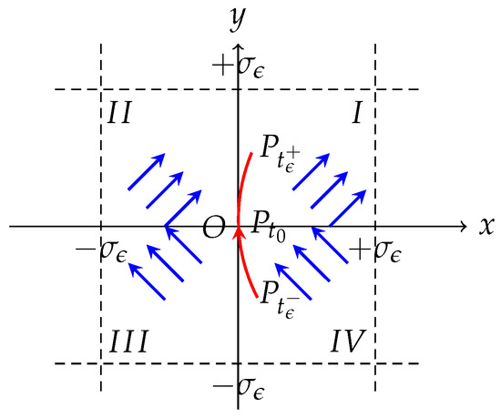
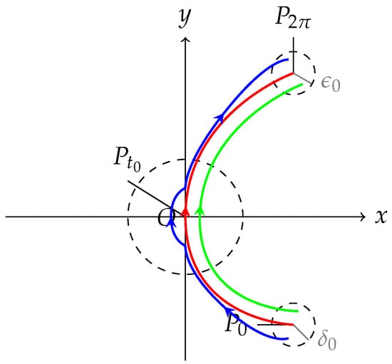
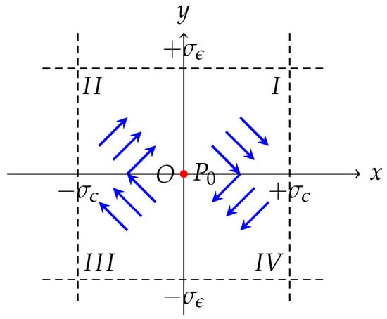
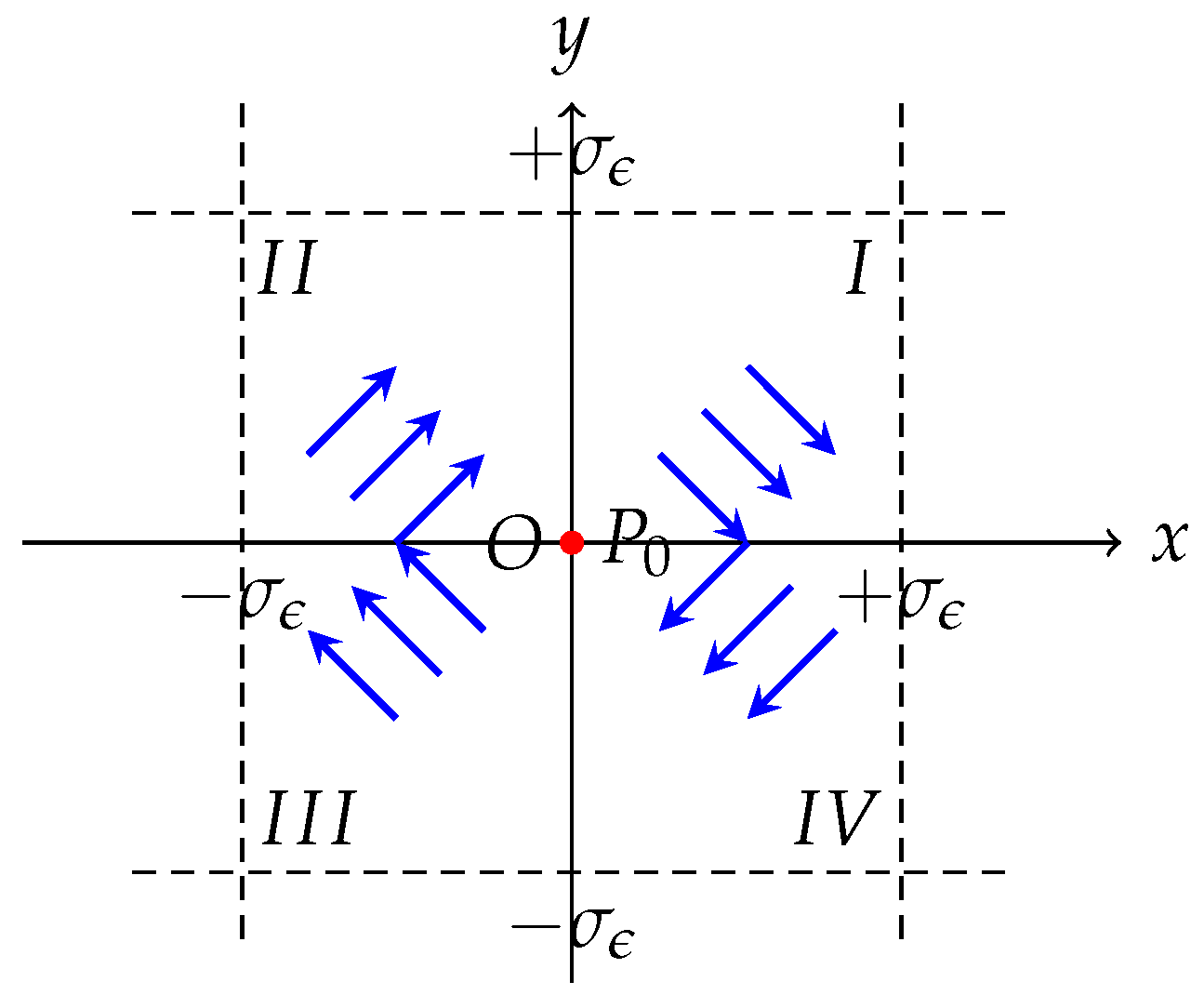
Finally, suppose that there exists $t_0\in [0,2\pi ]$ such that $P_{t_0}\in O$, and there does not exist $t_0^{\prime }\in [0,2\pi ]$ such that $P_{t_0^{\prime }}\in {\Sigma }_{0^{+}}\cup {\Sigma }_{0^{-}}$. Since the origin is the only possible sliding point, we define a square region $S_{{\sigma }_{ϵ}}$ that contains O where ${\sigma }_{ϵ}>0$ is small enough and name following four regions based on the intersection of $S_{{\sigma }_{ϵ}}$ with the four quadrants, as shown in Figure 3. The blue arrows in the figure indicate the approximate directions of the vector field in each region. According to Definition 1, we shall focus on the sign of the product of the vector field components along the normal vectors of the two coordinate axes in the subsequent analysis. By $\left(C_1\right)$ and (4), we have $\dot{y}>0$ in all regions $I,II,III,IV$; thus, there exist $t_{ϵ}^{-}<t_0$ and $t_{ϵ}^{+}>t_0$ sufficiently close to $t_0$ such that $P_t\in III,IV$ for $t\in [t_{ϵ}^{-},t_0)$ and $P_t\in I,II$ for $t\in (t_0,t_{ϵ}^{+}]$. However, analysis shows that the only path for point $P_{t_{ϵ}^{-}}$ moving to $P_{t_0}$ and then $P_{t_0}$ moving to $P_{t_{ϵ}^{+}}$ is entering region I from region $IV$ and being tangent to ${\Sigma }_0$ at the origin. Therefore, the corresponding solution $P_t$ exists and is unique for $t\in [t_{ϵ}^{-},t_{ϵ}^{+}]$. Based on the analysis, for the continuity of f, we only need to consider the situation as shown in Figure 4. □

To illustrate that condition $\left(G_2\right)$ rules out sliding behavior and ensures the continuity of the Poincaré map, we present a counterexample below. For this purpose, we impose the following situation

$$\left(C_5\right):g_{-}\left(0\right)<\underline{\beta }<\overline{\beta }<g_{+}\left(0\right),$$

which means

$$[\underline{\beta },\overline{\beta }]\subset (g_{-}\left(0\right),g_{+}\left(0\right)).$$

We then construct Figure 5 in analogy to the construction of Figure 3 in the proof of Lemma 1. By $\left(C_5\right)$ and (4), we obtain $\dot{y}>0$ in regions I and $IV$, whereas $\dot{y}<0$ is obtained in regions $II$ and $III$. Consequently, from a purely mathematical perspective without external perturbations, the solution of system (4) starting from the origin will remain at the origin permanently. The author draws an analogy between this phenomenon and isolated singular points in autonomous systems.

To establish the existence of $2\pi$ crossing periodic solutions, we further assume the following conditions to the Equation (2).

(H₀)

There exist positive numbers $p_1,p_2,q_1,q_2,A_1$ such that $g_{\pm }\left(x\right)$ satisfies:

$$q_1\le {\displaystyle \frac{g_{-}\left(x\right)}{x}}\le p_1,x\le -A_1;$$

$$q_2\le {\displaystyle \frac{g_{+}\left(x\right)}{x}}\le p_2,x\ge A_1.$$

(H₁)

There exists a positive integer m such that

$${\displaystyle \frac{1}{\sqrt{p_1}}}+{\displaystyle \frac{1}{\sqrt{p_2}}}={\displaystyle \frac{2}{m+1}},{\displaystyle \frac{1}{\sqrt{q_1}}}+{\displaystyle \frac{1}{\sqrt{q_2}}}={\displaystyle \frac{2}{m}}.$$

(H₂)

There exist positive constants $A_2$ and $B(>B_0)$ such that the following conditions hold

$$\left(1\right)g_{-}\left(x\right)-p_{1}x\ge B,x<-A_2,g_{+}\left(x\right)-p_{2}x\le -B,x>A_2;$$

$$\left(2\right)g_{-}\left(x\right)-q_{1}x\le -B,x<-A_2,g_{+}\left(x\right)-q_{2}x\ge B,x>A_2,$$

where $B_0={\displaystyle \frac{max(1,p_1^2,p_2^2)}{min(1,q_1^2,q_2^2)}}{\alpha }^2\beta \pi$ with $\alpha ={\mathrm{e}}^{(max\{p_1,p_2\}+2)\pi }$ and $\beta$ comes from (3).

3. Main Results

Now we apply the polar coordinate transformation

$$x\left(t\right)=r\left(t\right)cos\theta \left(t\right),y\left(t\right)=r\left(t\right)sin\theta \left(t\right)$$

(5)

to system (4). For $r\left(t\right)>0$ and $cos\theta \ne 0$, it can be rewritten as

$$\left\{\begin{array}{c}\dot{r}=rcos\theta sin\theta +\left[p\left(t\right)-g_{\pm }(rcos\theta )\right]sin\theta ,\hfill \\ \dot{\theta }=-{sin}^2\theta +{\displaystyle \frac{1}{r}}\left[p\left(t\right)-g_{\pm }(rcos\theta )\right]cos\theta .\hfill \end{array}\right.$$

(6)

Correspondingly, let $r\left(t\right)=r(t;r_0,{\theta }_0)$ and $\theta \left(t\right)=\theta (t;r_0,{\theta }_0)$ be the solution of (6) with the initial value $r\left(0\right)=r_0$ and $\theta \left(0\right)={\theta }_0$, where $r_0>0$ and ${\theta }_0\in \mathbb{R}$. And denote by $P(r_0,{\theta }_0;0,2\pi )$ the trajectory of the solution $(r(t;r_0,{\theta }_0),\theta (t;r_0,{\theta }_0))$ for $t\in [0,2\pi ]$.

Before stating the Lemma 2, we briefly explain why the global extendability of system solutions is necessary for our subsequent analysis. The Poincaré map on $[0,2\pi ]$ can only be well defined if all trajectories do not diverge in finite time; meanwhile, global existence also enables us to discuss the long-term recurrent motion of periodic solutions over infinite time.

Lemma 2.

Let $\left(H_0\right)$ hold; then, every solution of (4) is globally defined in both directions, i.e., the solution can be extended to $(-\infty ,+\infty )$.

Proof. 

Let $x\left(t\right)=x(t;x_0,y_0)$, $y\left(t\right)=y(t;x_0,y_0)$ be the solution of (4) satisfying the initial value $x\left(0\right)=x_0,y\left(0\right)=y_0$, and I denotes its maximal interval of existence. We first establish forward completeness by showing that $[0,+\infty )\subset I$.

Suppose, for contradiction, that $I\cap [0,+\infty )=[0,\gamma )$, where $\gamma$ is a constant satisfying $0<\gamma <\infty$. It is not difficult to deduce that

$$\underset{t\to {\gamma }^{-}}{lim}\left(\left|x\right(t\left)\right|+\left|y\right(t\left)\right|\right)=\infty .$$

(7)

On the other hand, by $\left(H_0\right)$, $g_{+}\left(x\right)$ has the same sign as x when $x\ge A_1$. Therefore, the corresponding potential function is bounded from below:

$$G_{+}\left(x\right)={\int }_0^x{g}_{+}\left(s\right)ds\ge -K,x>0,$$

(8)

where $K>0$ is a constant.

Next, multiply both sides of system (4) by y and note that ${\displaystyle \frac{dx}{dt}}=y$, which yields

$$y{\displaystyle \frac{dy}{dt}}+g_{+}\left(x\right){\displaystyle \frac{dx}{dt}}=p\left(t\right)y,x>0.$$

Integrating over the interval $[0,\gamma )$, we obtain

$$\begin{array}{c}\hfill {\int }_{y_0}^{y}ydy+{\int }_{x_0}^x{g}_{+}\left(x\right)dx={\int }_0^{t}p\left(t\right)ydt\\ \hfill {\displaystyle \frac{1}{2}}{y}^2+G_{+}\left(x\right)={\int }_0^{t}p\left(t\right)ydt+C,\end{array}$$

where $C={\displaystyle \frac{1}{2}}{y}_0^2+G_{+}\left(x_0\right)$.

Combining this with inequality (8), we get

$$\begin{array}{c}\hfill {\displaystyle \frac{1}{2}}{y}^2-K\le {\displaystyle \frac{1}{2}}{y}^2+G_{+}\left(x\right)\\ \hfill {\displaystyle \frac{1}{2}}{y}^2-K\le {\int }_0^t\left|p\left(t\right)\right|\left|y\right|dt+\left|C\right|\\ \hfill {\displaystyle \frac{1}{2}}{y}^2\le {\int }_0^t\left|p\left(t\right)\right|\left|y\right|dt+\left|C\right|+K.\end{array}$$

Let $u\left(t\right)={sup}_{0\le s\le t}\left|y\left(s\right)\right|$, it follows that

$${\displaystyle \frac{1}{2}}{y}^2\left(t\right)\le u\left(t\right){\int }_0^t\left|p\left(t\right)\right|dt+\left|C\right|+K.$$

If $y\left(t\right)$ is bounded on the interval I, its primitive function $x\left(t\right)$ is also bounded, which contradicts (7). Hence $y\left(t\right)$ must be unbounded. Further there exists a sequence $t_0<t_1<t_2<\cdots <t_k<\cdots \to \gamma$ such that $u\left(t_k\right)=\left|y\left(t_k\right)\right|\to +\infty$. Consequently,

$${\displaystyle \frac{1}{2}}{u}^2\left(t_k\right)\le C_{1}u\left(t_k\right)+C_0,$$

where $C_0=\left|C\right|+K$ and $C_1={\int }_0^{\gamma }\left|p\left(t\right)\right|dt$ are constants. This is a contradiction. Therefore, we conclude that $[0,+\infty )\subset I$.

The proof of the backward completeness of the solution is completely analogous and is, thus, omitted here. □

Lemma 3.

Let $\left(H_0\right)$ hold, there exists a positive number $R_1>0$ such that all orbits of (4) lying outside $S_{R_1}$ rotate clockwise around the origin O in the coordinate plane as the parameter t increases.

Proof. 

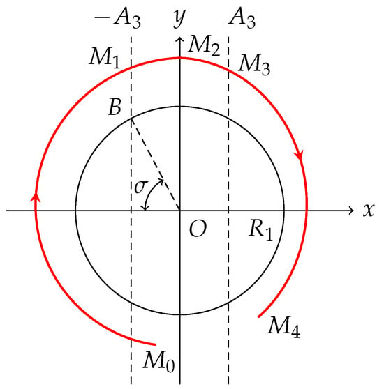
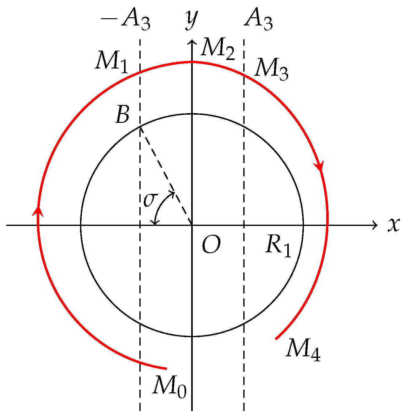
As shown in Figure 6, consider an orbit of (4) that lies outside the circle $S_{R_1}$, with the initial point $M_0$ and the terminal point $M_4$, and intersects ${\Sigma }_0$ transversally at $M_2$. From $\left(H_0\right)$, we obtain

$$\underset{x\to -\infty }{lim}{g}_{-}\left(x\right)=-\infty ,\underset{x\to +\infty }{lim}{g}_{+}\left(x\right)=+\infty .$$

Hence, there exists a positive constant $A_3>0$ such that

$$g_{-}\left(x\right)<\underline{\beta },x<-A_3;g_{+}\left(x\right)>\overline{\beta },x>A_3,$$

(9)

where $\underline{\beta }$ and $\overline{\beta }$ come from (3). Accordingly, the following inequalities hold:

$$\left\{\begin{array}{cc}\left[p\left(t\right)-g_{-}(rcos\theta )\right]cos\theta <0,\hfill & t\in [0,2\pi ],x<-A_3,\hfill \\ \left[p\left(t\right)-g_{+}(rcos\theta )\right]cos\theta <0,\hfill & t\in [0,2\pi ],x>A_3.\hfill \end{array}\right.$$

(10)

Combining Equations (6) and (10), we conclude that for $\left|x\right|>A_3$,

$$\dot{\theta }=-{sin}^2\theta +{\displaystyle \frac{1}{r}}\left[p\left(t\right)-g_{\pm }(rcos\theta )\right]cos\theta <0.$$

For $0<\left|x\right|<A_3$, let B stand for the intersection of the line $x=-A_3$ and the circle $S_{R_1}$, and let $\sigma$ be the angle between the ray $OB$ and the negative x-axis. Clearly, $sin\sigma ={\displaystyle \frac{\sqrt{R_1^2-A_3^2}}{R_1}}$.

Suppose $R_1>A_3.$ Substituting the above relation into (6) yields

$$\begin{array}{cc}\hfill \dot{\theta }& =-{sin}^2\theta +{\displaystyle \frac{1}{r}}\left[p\left(t\right)-g_{\pm }(rcos\theta )\right]cos\theta \hfill \\ & <-{\left({\displaystyle \frac{\sqrt{R_1^2-A_3^2}}{R_1}}\right)}^2+{\displaystyle \frac{\delta }{R_1}}\hfill \\ & =-{\displaystyle \frac{R_1^2-\delta R_1-A_3^2}{R_1^2}},\hfill \end{array}$$

where $\delta =\beta +max\left\{\underset{-A_3<x<0}{sup}|g_{-}\left(x\right)|,\underset{0<x<A_3}{sup}\left|g_{+}\left(x\right)\right|\right\}$, with $\beta$ given in (3).

Consequently, if $R_1>{\displaystyle \frac{1}{2}}\left(\delta +\sqrt{4A_3^2+{\delta }^2}\right)$, we have $\dot{\theta }<0$. This finishes the proof. □

Lemma 4.

Let $\left(H_0\right)$ hold, there exists $R_2>0$ such that when $r_0>R_2$, the orbit $P(r_0,{\theta }_0;0,2\pi )$ of (4) is entirely contained in the annulus

$$D_0=\left\{(r,\theta )\mid {\displaystyle \frac{r_0}{\alpha }}<r<\alpha r_0\right\}.$$

Proof. 

By $\left(H_0\right)$, we have that

$$\left\{\begin{array}{c}0<{\displaystyle \frac{g_{-}\left(x\right)}{x}}\le p_1,x\le -A_1,\hfill \\ 0<{\displaystyle \frac{g_{+}\left(x\right)}{x}}\le p_2,x\ge A_1.\hfill \end{array}\right.$$

(11)

Denote by $\delta =\beta +max\left\{\underset{-A_1<x<0}{sup}|g_{-}\left(x\right)|,\underset{0<x<A_1}{sup}|g_{+}\left(x\right)|\right\}$. Suppose $r\left(t\right)>2\delta$. We divide the discussion into two cases according to (6).

On one hand, for $0<\left|x\right|<A_1$,

$$\begin{array}{cc}\hfill |\dot{r}\left(t\right)|& \le |rcos\theta sin\theta |+|p\left(t\right)sin\theta |+\left|g_{\pm }(rcos\theta )sin\theta \right|,\hfill \\ \hfill & \le {\displaystyle \frac{1}{2}}r\left(t\right)+\delta <r\left(t\right).\hfill \end{array}$$

On the other hand, for $\left|x\right|\ge A_1$ combined with (11),

$$\begin{array}{cc}\hfill |\dot{r}\left(t\right)|& \le |rcos\theta sin\theta |+|p\left(t\right)sin\theta |+\left|{\displaystyle \frac{g_{\pm }(rcos\theta )}{rcos\theta }}\right||rcos\theta sin\theta |,\hfill \\ \hfill & \le {\displaystyle \frac{1}{2}}r\left(t\right)+\beta +{\displaystyle \frac{1}{2}}max\{p_1,p_2\}r\left(t\right),\hfill \\ \hfill & <{\displaystyle \frac{1}{2}}\left(max\{p_1,p_2\}+2\right)r\left(t\right).\hfill \end{array}$$

Therefore, let $\alpha ={\mathrm{e}}^{(max\{p_1,p_2\}+2)\pi }$ and choose $R_2=2\delta \alpha$. Then for $r_0>R_2$, we have

$$|\dot{r}\left(t\right)|<{\displaystyle \frac{1}{2}}\left(max\{p_1,p_2\}+2\right)r\left(t\right),t\in [0,2\pi ],$$

which implies

$${\displaystyle \frac{r_0}{\alpha }}<r\left(t\right)<\alpha r_0,t\in [0,2\pi ].$$

This completes the proof. □

Theorem 2.

Let $\left(H_0\right)$,$\left(H_1\right)$ and $\left(H_2\right)$ hold; the discontinuous Duffing Equation (2) admits at least one $2\pi$ crossing periodic solution.

Proof. 

By Lemma 3, there exists $R_1>0$ such that all orbits of (4) outside $S_{R_1}$ rotate clockwise around the origin O. Furthermore, by Lemma 4, there exist constants $R_2>0$ and $\alpha >0$ such that if $r_0>R_2$, the orbit $P(r_0,{\theta }_0;0,2\pi )$ is entirely contained in the annulus

$$D_0:\{(r,\theta )\mid {\displaystyle \frac{r_0}{\alpha }}<r<\alpha r_0\}.$$

Next, we estimate the range of time T required for the orbit $P(r_0,{\theta }_0;0,2\pi )$ to complete one full circle around the origin. For convenience, define

$$\left\{\begin{array}{cc}{g}_{-}\left(x\right)=p_{1}x+f_1\left(x\right),\hfill & x<0,\hfill \\ g_{+}\left(x\right)=p_{2}x+f_2\left(x\right),\hfill & x>0.\hfill \end{array}\right.$$

(12)

$$\left\{\begin{array}{cc}{g}_{-}\left(x\right)=q_{1}x+h_1\left(x\right),\hfill & x<0,\hfill \\ g_{+}\left(x\right)=q_{2}x+h_2\left(x\right),\hfill & x>0.\hfill \end{array}\right.$$

(13)

By $\left(H_0\right),\left(H_2\right)$, there exist constants $A>max\{A_1,A_2\}$ and $B>0$ such that

$$\left\{\begin{array}{cc}{f}_1\left(x\right)\ge B,\hfill & x<-A,\hfill \\ f_2\left(x\right)\le -B,\hfill & x>A.\hfill \end{array}\right.$$

(14)

$$\left\{\begin{array}{cc}{h}_1\left(x\right)\le -B,\hfill & x<-A,\hfill \\ h_2\left(x\right)\ge B,\hfill & x>A.\hfill \end{array}\right.$$

(15)

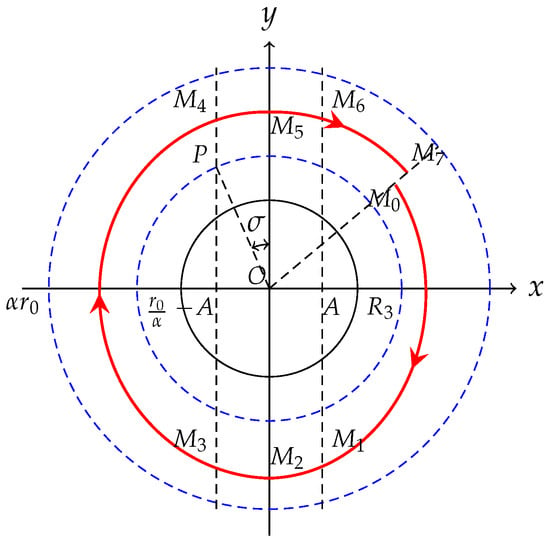
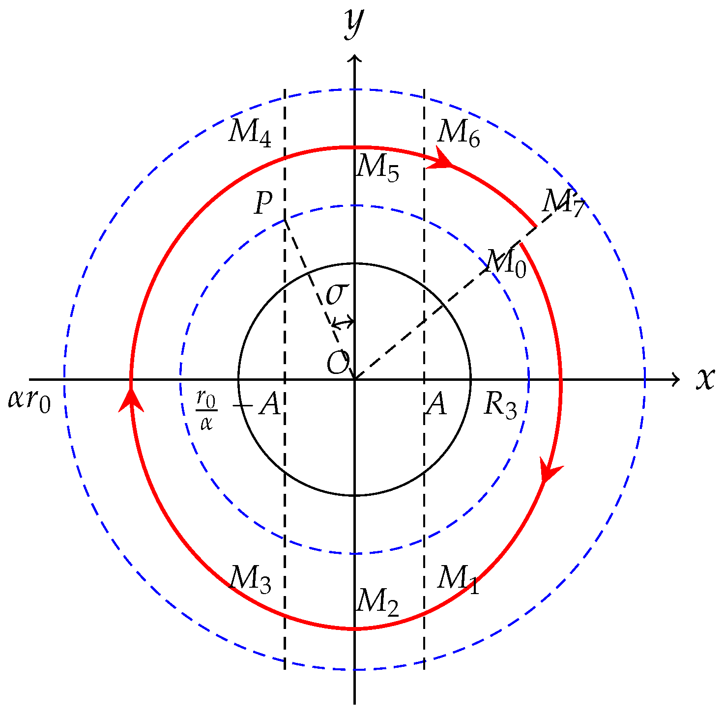
Now we choose a sufficiently large $R_3>max\{R_2,A\}$ such that the annulus $D_0$ lies outside $S_{R_1}$ whenever $r_0>R_3$. As illustrated in Figure 7, without loss of generality, let $M_0(r_0,{\theta }_0)$ be a point on the right side of the line $x=A$ outside $S_{R_3}$. The orbit starting from $M_0$ at time $t_0=0$ rotates clockwise around the origin for one full cycle, intersecting the lines $x=A$, ${\Sigma }_{0^{-}}$, $x=-A$, $x=-A$, ${\Sigma }_{0^{+}}$, $x=A$ and the ray $\theta ={\theta }_0$ successively at points $M_1,M_2,M_3,M_4,M_5,M_6,M_7$, where the polar angles corresponding to $O{M}_1,O{M}_2,O{M}_3,O{M}_4,O{M}_5,O{M}_6,O{M}_7$ are ${\theta }_1,{\theta }_2,{\theta }_3,{\theta }_4,{\theta }_5,{\theta }_6,{\theta }_7$ respectively, and the corresponding times are $t_1,t_2,t_3,t_4,t_5,t_6,t_7$, where ${\theta }_2=-\pi /2$ and ${\theta }_5=-3\pi /2$.

Using Equation (6) together with (12) and (14), we obtain

$$\begin{array}{cc}\hfill t_1-t_0& ={\int }_{{\theta }_1}^{{\theta }_0}{\displaystyle \frac{d\theta }{{sin}^2\theta +\frac{1}{r}(g_{+}(rcos\theta )-p\left(t\right))cos\theta }}\hfill \\ \hfill & ={\int }_{{\theta }_1}^{{\theta }_0}{\displaystyle \frac{d\theta }{{sin}^2\theta +p_2{cos}^2\theta +\frac{1}{r}{f}_2(rcos\theta )cos\theta -\frac{1}{r}p\left(t\right)cos\theta }}\hfill \\ \hfill & \ge {\int }_{{\theta }_1}^{{\theta }_0}{\displaystyle \frac{d\theta }{{sin}^2\theta +p_2{cos}^2\theta -\frac{B}{\alpha r_0}cos\theta +\frac{\alpha \beta }{r_0}}}.\hfill \\ \hfill t_7-t_6& \ge {\int }_{{\theta }_7}^{{\theta }_6}{\displaystyle \frac{d\theta }{{sin}^2\theta +p_2{cos}^2\theta -\frac{B}{\alpha r_0}cos\theta +\frac{\alpha \beta }{r_0}}}.\hfill \end{array}$$

Note that ${\theta }_7+2\pi ={\theta }_0$, by the periodicity of the integrand then

$$\begin{array}{cc}\hfill (t_1-t_0)+(t_7-t_6)& \ge {\int }_{{\theta }_1}^{{\theta }_6+2\pi }{\displaystyle \frac{d\theta }{{sin}^2\theta +p_2{cos}^2\theta -\frac{B}{\alpha r_0}cos\theta +\frac{\alpha \beta }{r_0}}}\hfill \\ \hfill & \ge {\int }_{{\theta }_1}^{{\theta }_6+2\pi }{\displaystyle \frac{d\theta }{{sin}^2\theta +p_2{cos}^2\theta }}\hfill \\ \hfill & +{\int }_{{\theta }_1}^{{\theta }_6+2\pi }{\displaystyle \frac{1}{{({sin}^2\theta +p_2{cos}^2\theta )}^2}}\left({\displaystyle \frac{B}{\alpha r_0}}cos\theta -{\displaystyle \frac{\alpha \beta }{r_0}}\right)d\theta +L\left(r_0\right)\hfill \\ \hfill & \ge {\int }_{{\theta }_1}^{{\theta }_6+2\pi }{\displaystyle \frac{d\theta }{{sin}^2\theta +p_2{cos}^2\theta }}+{\displaystyle \frac{B}{max(1,p_2^2)\alpha r_0}}{\int }_{-{\displaystyle \frac{\pi }{2}}+\sigma }^{{\displaystyle \frac{\pi }{2}}-\sigma }cos\theta d\theta \hfill \\ \hfill & -{\displaystyle \frac{\alpha \beta \pi }{min(1,p_2^2)r_0}}+L\left(r_0\right)\hfill \end{array}$$

and

$$\begin{array}{cc}\hfill {\displaystyle \frac{B}{max(1,p_2^2)\alpha r_0}}{\int }_{-{\displaystyle \frac{\pi }{2}}+\sigma }^{{\displaystyle \frac{\pi }{2}}-\sigma }cos\theta d\theta & ={\displaystyle \frac{2B}{max(1,p_2^2)\alpha r_0}}\sqrt{1-{\left({\displaystyle \frac{\alpha A}{r_0}}\right)}^2}\hfill \\ \hfill & ={\displaystyle \frac{2B}{max(1,p_2^2)\alpha r_0}}-{\displaystyle \frac{B\alpha A^2}{max(1,p_2^2)r_0^3}}+o\left({\displaystyle \frac{1}{r_0^3}}\right)\hfill \\ \hfill & ={\displaystyle \frac{2B}{max(1,p_2^2)\alpha r_0}}+o\left({\displaystyle \frac{1}{r_0}}\right),\hfill \end{array}$$

where $\sigma$ denotes the acute angle between the ray $OP$ and the positive y-axis, as illustrated in Figure 7. As $r_0\to \infty$, the notation $o(1/r_0)$ represents an infinitesimal quantity of higher order than $1/r_0$.

Substituting this into the previous estimate, we obtain

$$\begin{array}{cc}\hfill (t_1-t_0)+(t_7-t_6)& \ge {\int }_{{\theta }_1}^{{\theta }_6+2\pi }{\displaystyle \frac{d\theta }{{sin}^2\theta +p_2{cos}^2\theta }}+{\displaystyle \frac{2B}{max(1,p_2^2)\alpha r_0}}-{\displaystyle \frac{\alpha \beta \pi }{min(1,p_2^2)r_0}}+o\left({\displaystyle \frac{1}{r_0}}\right),\hfill \end{array}$$

where

$$\begin{array}{cc}\hfill L\left(r_0\right)& ={\int }_{{\theta }_1}^{{\theta }_6+2\pi }{\displaystyle \frac{{\left(\frac{B}{\alpha r_0}cos\theta -\frac{\alpha \beta }{r_0}\right)}^{2}d\theta }{{({sin}^2\theta +p_2{cos}^2\theta )}^2\left({sin}^2\theta +p_2{cos}^2\theta -\frac{B}{\alpha r_0}cos\theta +\frac{\alpha \beta }{r_0}\right)}}\hfill \\ \hfill & ={\displaystyle \frac{1}{r_0^2}}{\int }_{{\theta }_1}^{{\theta }_6+2\pi }{\displaystyle \frac{{\left(\frac{B}{\alpha }cos\theta -\alpha \beta \right)}^{2}d\theta }{{({sin}^2\theta +p_2{cos}^2\theta )}^2\left[({sin}^2\theta +p_2{cos}^2\theta )-\frac{B}{\alpha r_0}cos\theta +\frac{\alpha \beta }{r_0}\right]}},\hfill \\ \hfill \left|L\right(r_0\left)\right|& \le {\displaystyle \frac{\pi }{r_0^2}}{\displaystyle \frac{{\left(\frac{B}{\alpha }+\alpha \beta \right)}^2}{min(1,p_2^2)\left(min(1,p_2)-\frac{B}{\alpha r_0}\right)}}.\hfill \end{array}$$

Similarly, we have that

$$\begin{array}{cc}\hfill t_4-t_3& ={\int }_{{\theta }_4}^{{\theta }_3}{\displaystyle \frac{d\theta }{{sin}^2\theta +\frac{1}{r}(g_{-}(rcos\theta )-p\left(t\right))cos\theta }}\hfill \\ \hfill & ={\int }_{{\theta }_4}^{{\theta }_3}{\displaystyle \frac{d\theta }{{sin}^2\theta +p_1{cos}^2\theta +\frac{1}{r}{f}_1(rcos\theta )cos\theta -\frac{1}{r}p\left(t\right)cos\theta }}\hfill \\ \hfill & \ge {\int }_{{\theta }_4}^{{\theta }_3}{\displaystyle \frac{d\theta }{{sin}^2\theta +p_1{cos}^2\theta +\frac{B}{\alpha r_0}cos\theta +\frac{\alpha \beta }{r_0}}}\hfill \\ \hfill & \ge {\int }_{{\theta }_4}^{{\theta }_3}{\displaystyle \frac{d\theta }{{sin}^2\theta +p_1{cos}^2\theta }}-{\int }_{{\theta }_4}^{{\theta }_3}{\displaystyle \frac{1}{{({sin}^2\theta +p_1{cos}^2\theta )}^2}}\left({\displaystyle \frac{B}{\alpha r_0}}cos\theta +{\displaystyle \frac{\alpha \beta }{r_0}}\right)d\theta +L_1\left(r_0\right)\hfill \\ \hfill & \ge {\int }_{{\theta }_4}^{{\theta }_3}{\displaystyle \frac{d\theta }{{sin}^2\theta +p_1{cos}^2\theta }}-{\displaystyle \frac{B}{max(1,p_1^2)\alpha r_0}}{\int }_{-{\displaystyle \frac{3\pi }{2}}+\sigma }^{-{\displaystyle \frac{\pi }{2}}-\sigma }cos\theta d\theta -{\displaystyle \frac{\alpha \beta \pi }{min(1,p_1^2)r_0}}+L_1\left(r_0\right)\hfill \\ \hfill & \ge {\int }_{{\theta }_4}^{{\theta }_3}{\displaystyle \frac{d\theta }{{sin}^2\theta +p_1{cos}^2\theta }}+{\displaystyle \frac{2B}{max(1,p_1^2)\alpha r_0}}-{\displaystyle \frac{\alpha \beta \pi }{min(1,p_1^2)r_0}}+o\left({\displaystyle \frac{1}{r_0}}\right),\hfill \end{array}$$

where

$$\begin{array}{cc}\hfill L_1\left(r_0\right)& ={\int }_{{\theta }_4}^{{\theta }_3}{\displaystyle \frac{{\left(\frac{B}{\alpha r_0}cos\theta +\frac{\alpha \beta }{r_0}\right)}^{2}d\theta }{{({sin}^2\theta +p_1{cos}^2\theta )}^2\left({sin}^2\theta +p_1{cos}^2\theta +\frac{B}{\alpha r_0}cos\theta +\frac{\alpha \beta }{r_0}\right)}}\hfill \\ \hfill & ={\displaystyle \frac{1}{r_0^2}}{\int }_{{\theta }_4}^{{\theta }_3}{\displaystyle \frac{{\left(\frac{B}{\alpha }cos\theta +\alpha \beta \right)}^{2}d\theta }{{({sin}^2\theta +p_1{cos}^2\theta )}^2\left[({sin}^2\theta +p_1{cos}^2\theta )+\frac{B}{\alpha r_0}cos\theta +\frac{\alpha \beta }{r_0}\right]}},\hfill \\ \hfill |L_1\left(r_0\right)|& \le {\displaystyle \frac{\pi }{r_0^2}}{\displaystyle \frac{{\left(\frac{B}{\alpha }+\alpha \beta \right)}^2}{min(1,p_1^2)\left(min(1,p_1)-\frac{B}{\alpha r_0}\right)}}.\hfill \end{array}$$

Furthermore,

$$\begin{array}{cc}\hfill (t_2-t_1)+(t_6-t_5)& =\left({\int }_{{\theta }_2}^{{\theta }_1}+{\int }_{{\theta }_6}^{{\theta }_5}\right){\displaystyle \frac{d\theta }{{sin}^2\theta +p_2{cos}^2\theta +\frac{1}{r}[f_2(rcos\theta )-p\left(r\right)]cos\theta }}\hfill \\ \hfill & \ge \left({\int }_{{\theta }_2}^{{\theta }_1}+{\int }_{{\theta }_6}^{{\theta }_5}\right){\displaystyle \frac{d\theta }{{sin}^2\theta +p_2{cos}^2\theta +\frac{\alpha (f_2+\beta )}{r_0}}}\hfill \\ \hfill & \ge \left({\int }_{{\theta }_2}^{{\theta }_1}+{\int }_{{\theta }_6}^{{\theta }_5}\right){\displaystyle \frac{d\theta }{{sin}^2\theta +p_2{cos}^2\theta }}\hfill \\ \hfill & -{\displaystyle \frac{\alpha (f_2+\beta )}{r_0}}\left({\int }_{{\theta }_2}^{{\theta }_1}+{\int }_{{\theta }_6}^{{\theta }_5}\right){\displaystyle \frac{d\theta }{{\left({sin}^2\theta +p_2{cos}^2\theta \right)}^2}}+o\left({\displaystyle \frac{1}{r_0}}\right)\hfill \\ \hfill & \ge \left({\int }_{{\theta }_2}^{{\theta }_1}+{\int }_{{\theta }_6}^{{\theta }_5}\right){\displaystyle \frac{d\theta }{{sin}^2\theta +p_2{cos}^2\theta }}+o\left({\displaystyle \frac{1}{r_0}}\right),\hfill \end{array}$$

where $f_2=\underset{0<x<A}{sup}\left|f_2\left(x\right)\right|.$ And

$$\begin{array}{cc}\hfill & \left|{\displaystyle \frac{\alpha (f_2+\beta )}{r_0}}\left({\int }_{{\theta }_2}^{{\theta }_1}+{\int }_{{\theta }_6}^{{\theta }_5}\right){\displaystyle \frac{d\theta }{{\left({sin}^2\theta +p_2{cos}^2\theta \right)}^2}}\right|\hfill \\ \hfill & \le {\displaystyle \frac{\alpha (f_2+\beta )}{r_{0}min\{1,p_2^2\}}}\left({\int }_{-{\displaystyle \frac{\pi }{2}}}^{-{\displaystyle \frac{\pi }{2}}+\sigma }+{\int }_{-{\displaystyle \frac{3\pi }{2}}-\sigma }^{-{\displaystyle \frac{3\pi }{2}}}\right)d\theta \hfill \\ \hfill & \le {\displaystyle \frac{\alpha (f_2+\beta )}{r_{0}min\{1,p_2^2\}}}\left({\int }_{-{\displaystyle \frac{\pi }{2}}}^{-{\displaystyle \frac{\pi }{2}}+\sigma }+{\int }_{-{\displaystyle \frac{3\pi }{2}}-\sigma }^{-{\displaystyle \frac{3\pi }{2}}}\right)|2sin\theta |d\theta \hfill \\ \hfill & ={\displaystyle \frac{4\alpha (f_2+\beta )}{r_{0}min\{1,p_2^2\}}}sin\sigma \hfill \\ \hfill & ={\displaystyle \frac{4{\alpha }^2(f_2+\beta )A}{r_0^{2}min\{1,p_2^2\}}}.\hfill \end{array}$$

Similarly, for the remaining time intervals, we have

$$\begin{array}{cc}\hfill (t_3-t_2)+(t_5-t_4)& =\left({\int }_{{\theta }_3}^{{\theta }_2}+{\int }_{{\theta }_5}^{{\theta }_4}\right){\displaystyle \frac{d\theta }{{sin}^2\theta +p_1{cos}^2\theta +\frac{1}{r}[f_1(rcos\theta )-p\left(r\right)]cos\theta }}\hfill \\ \hfill & \ge \left({\int }_{{\theta }_3}^{{\theta }_2}+{\int }_{{\theta }_5}^{{\theta }_4}\right){\displaystyle \frac{d\theta }{{sin}^2\theta +p_1{cos}^2\theta }}+o\left({\displaystyle \frac{1}{r_0}}\right).\hfill \end{array}$$

Combining all the above interval estimates, we further derive the lower bound of the total time T:

$$\begin{array}{cc}\hfill T=t_7-t_0& \ge {\int }_{-{\displaystyle \frac{\pi }{2}}}^{{\displaystyle \frac{\pi }{2}}}{\displaystyle \frac{d\theta }{{sin}^2\theta +p_2{cos}^2\theta }}+{\int }_{-{\displaystyle \frac{3}{2}}\pi }^{-{\displaystyle \frac{\pi }{2}}}{\displaystyle \frac{d\theta }{{sin}^2\theta +p_1{cos}^2\theta }}\hfill \\ \hfill & +\left[{\displaystyle \frac{2B}{max(1,p_2^2)\alpha }}+{\displaystyle \frac{2B}{max(1,p_1^2)\alpha }}-{\displaystyle \frac{\alpha \beta \pi }{min(1,p_1^2)}}-{\displaystyle \frac{\alpha \beta \pi }{min(1,p_2^2)}}\right]{\displaystyle \frac{1}{r_0}}+o\left({\displaystyle \frac{1}{r_0}}\right)\hfill \\ \hfill & =\left({\displaystyle \frac{\pi }{\sqrt{p_1}}}+{\displaystyle \frac{\pi }{\sqrt{p_2}}}\right)+\left[{\displaystyle \frac{2B}{max(1,p_2^2)\alpha }}+{\displaystyle \frac{2B}{max(1,p_1^2)\alpha }}-{\displaystyle \frac{\alpha \beta \pi }{min(1,p_1^2)}}-{\displaystyle \frac{\alpha \beta \pi }{min(1,p_2^2)}}\right]{\displaystyle \frac{1}{r_0}}\hfill \\ \hfill & +o\left({\displaystyle \frac{1}{r_0}}\right)\hfill \\ \hfill & \ge {\displaystyle \frac{2\pi }{m+1}}+\left[{\displaystyle \frac{2B}{max(1,p_2^2)\alpha }}+{\displaystyle \frac{2B}{max(1,p_1^2)\alpha }}-{\displaystyle \frac{\alpha \beta \pi }{min(1,p_1^2)}}-{\displaystyle \frac{\alpha \beta \pi }{min(1,p_2^2)}}\right]{\displaystyle \frac{1}{r_0}}+o\left({\displaystyle \frac{1}{r_0}}\right).\hfill \end{array}$$

$$T\ge {\displaystyle \frac{2\pi }{m+1}}+\left[{\displaystyle \frac{2B}{max(1,p_2^2)\alpha }}+{\displaystyle \frac{2B}{max(1,p_1^2)\alpha }}-{\displaystyle \frac{\alpha \beta \pi }{min(1,p_1^2)}}-{\displaystyle \frac{\alpha \beta \pi }{min(1,p_2^2)}}\right]{\displaystyle \frac{1}{r_0}}+o\left({\displaystyle \frac{1}{r_0}}\right).$$

(16)

Using the same method and combining (13) and (15), we also obtain

$$T\le {\displaystyle \frac{2\pi }{m}}-\left[{\displaystyle \frac{2B}{max(1,q_2^2)\alpha }}+{\displaystyle \frac{2B}{max(1,q_1^2)\alpha }}-{\displaystyle \frac{\alpha \beta \pi }{min(1,q_1^2)}}-{\displaystyle \frac{\alpha \beta \pi }{min(1,q_2^2)}}\right]{\displaystyle \frac{1}{r_0}}+o\left({\displaystyle \frac{1}{r_0}}\right).$$

(17)

Note that $p_1\ge q_1$, $p_2\ge q_2$. It follows from $B>B_0$ that

$$\begin{array}{c}{\displaystyle \frac{2B}{max(1,p_2^2)\alpha }}+{\displaystyle \frac{2B}{max(1,p_1^2)\alpha }}-{\displaystyle \frac{\alpha \beta \pi }{min(1,p_1^2)}}-{\displaystyle \frac{\alpha \beta \pi }{min(1,p_2^2)}}>0,\\ {\displaystyle \frac{2B}{max(1,q_2^2)\alpha }}+{\displaystyle \frac{2B}{max(1,q_1^2)\alpha }}-{\displaystyle \frac{\alpha \beta \pi }{min(1,q_1^2)}}-{\displaystyle \frac{\alpha \beta \pi }{min(1,q_2^2)}}>0.\end{array}$$

Further we have that

$${\displaystyle \frac{2\pi }{m+1}}<T<{\displaystyle \frac{2\pi }{m}}.$$

In conclusion, when $(\xi ,\eta )\in S_{r_0}$, the orbit $P(r_0,{\theta }_0;0,2\pi )$ rotates clockwise around the origin for a number of cycles greater than m and less than $m+1$. This implies that the initial point $P_0$ and the terminal point $P_{2\pi }$ cannot lie on the same ray emanating from the origin. Hence, for any $\lambda \ge 1$ and $(\xi ,\eta )\in S_{r_0}$, the map f satisfies the boundary condition $(u,v)\ne \lambda (\xi ,\eta ).$ Moreover, it follows from Lemma 1 that f is continuous on $B_{r_0}$. By the Poincaré–Bohl Theorem (Theorem 1), f admits at least one fixed point in $B_{r_0}$, which corresponds to a $2\pi$ crossing periodic solution of Equation (2). This completes the proof. □

Theorem 3.

If we change Theorem 2’s condition $\left(H_1\right)$ into $\left(H_1^{\prime }\right)$ as below

$\left(H_1^{\prime }\right)$

There exists a positive integer m such that

$${\displaystyle \frac{2}{m+1}}<{\displaystyle \frac{1}{\sqrt{p_1}}}+{\displaystyle \frac{1}{\sqrt{p_2}}}\le {\displaystyle \frac{1}{\sqrt{q_1}}}+{\displaystyle \frac{1}{\sqrt{q_2}}}<{\displaystyle \frac{2}{m}},$$

then the conclusion of Theorem 2 still holds.

Proof. 

Actually, by $\left(H_1^{\prime }\right)$ we can still find $p_1^{*},p_2^{*},q_1^{*},q_2^{*}$ such that $p_1^{*}>p_1$, $p_2^{*}>p_2$, $0<q_1^{*}<q_1$, $0<q_2^{*}<q_2$ and

$${\displaystyle \frac{1}{\sqrt{p_1^{*}}}}+{\displaystyle \frac{1}{\sqrt{p_2^{*}}}}={\displaystyle \frac{2}{m+1}},{\displaystyle \frac{1}{\sqrt{q_1^{*}}}}+{\displaystyle \frac{1}{\sqrt{q_2^{*}}}}={\displaystyle \frac{2}{m}}.$$

Additionally, the inequalities required in $\left(H_0\right)$ and $\left(H_2\right)$ still hold for $p_1^{*},p_2^{*},q_1^{*},q_2^{*}.$ □

Theorem 4.

Suppose we replace the conditions $\left(H_0\right)$–$\left(H_2\right)$ of Theorem 2 with the following conditions $\left(H_0^{″}\right)$, $\left(H_1^{″}\right)$, and $\left(H_2^{″}\right)$. Then the conclusion of Theorem 2 still holds.

$\left(H_0^{″}\right)$

There exist positive constants $p_1,p_2,A_1$ such that the functions $g_{\pm }\left(x\right)$ satisfy

$$0<{\displaystyle \frac{g_{-}\left(x\right)}{x}}\le p_1,x\le -A_1;$$

$$0<{\displaystyle \frac{g_{+}\left(x\right)}{x}}\le p_2,x\ge A_1.$$

$\left(H_1^{″}\right)$

The following equality holds

$${\displaystyle \frac{1}{\sqrt{p_1}}}+{\displaystyle \frac{1}{\sqrt{p_2}}}=2.$$

$\left(H_2^{″}\right)$

There exist positive constants $A_2$ and $B>B_1$ such that

$$\left(1\right)g_{-}\left(x\right)-p_{1}x\ge B,x<-A_2,g_{+}\left(x\right)-p_{2}x\le -B,x>A_2;$$

$$\left(2\right)g_{-}\left(x\right)\le -B,x<-A_2,g_{+}\left(x\right)\ge B,x>A_2,$$

where $B_1={\displaystyle \frac{max(1,p_1^2,p_2^2)}{min(1,p_1^2,p_2^2)}}{\alpha }^2\beta \pi$.

Proof. 

We first verify that Lemmas 2–4 still hold under the modified hypotheses. Detailed proofs for these lemmas under the original condition $\left(H_0\right)$ have been established previously, so we only check the crucial estimates to avoid redundant arguments.

Although the inequality (8) in Lemma 2 fails to hold merely under $\left(H_0^{″}\right)$, it is recovered via item (2) of $\left(H_2^{″}\right)$, which preserves the validity of Lemma 2. Similarly, relation (9) in Lemma 3 holds owing to condition $\left(H_2^{″}\right)\left(2\right)$, and the key inequality (11) required in the proof of Lemma 4 is directly guaranteed by $\left(H_0^{″}\right)$.

We then adopt the integral estimation techniques developed in the proof of Theorem 2 to derive the following lower-bound inequality:

$$T\ge 2\pi +\left[{\displaystyle \frac{2B}{max\{1,p_2^2\}\alpha }}+{\displaystyle \frac{2B}{max\{1,p_1^2\}\alpha }}-{\displaystyle \frac{\alpha \beta \pi }{min\{1,p_1^2\}}}-{\displaystyle \frac{\alpha \beta \pi }{min\{1,p_2^2\}}}\right]{\displaystyle \frac{1}{r_0}}+o\left({\displaystyle \frac{1}{r_0}}\right).$$

(18)

To this end, it suffices to adopt the expressions (12) and (14). By repeating the derivation arguments used in the proof of Theorem 2, we obtain the crucial inequality (16). Furthermore, the condition $\left(H_1^{″}\right)$ imposes the restriction $m=0$, which eventually establishes the inequality (18).

If we put $B>B_1$, then we get

$$\begin{array}{c}\hfill T>2\pi .\end{array}$$

Combining the analysis in the final part of Theorem 2, we conclude that, under the current settings, the orbit $P(r_0,{\theta }_0;0,2\pi )$ rotates clockwise around the origin by less than one full circle. Consequently, the initial point $P_0$ and the endpoint $P_{2\pi }$ cannot lie on the same ray emanating from the origin, which implies that the conclusion of Theorem 2 still holds true. □

Theorem 5.

If we change Theorem 4’s condition $\left(H_1^{″}\right)$ into $\left(H_1^{‴}\right)$ as below

$\left(H_1^{‴}\right)$

$${\displaystyle \frac{1}{\sqrt{p_1}}}+{\displaystyle \frac{1}{\sqrt{p_2}}}>2,$$

then the conclusion still holds.

Proof. 

Actually, by $\left(H_1^{‴}\right)$ we can find $p_1^{*},p_2^{*}$ such that $p_1^{*}>p_1$, $p_2^{*}>p_2$ and

$${\displaystyle \frac{1}{\sqrt{p_1^{*}}}}+{\displaystyle \frac{1}{\sqrt{p_2^{*}}}}=2.$$

In addition, the inequalities required in $\left(H_0^{″}\right)$, $\left(H_2^{″}\right)$ also hold for $p_1^{*},p_2^{*}$. □

4. An Example

Consider a discontinuous Duffing Equation (2) with $g_{\pm }\left(x\right)$ and $p\left(t\right)$ defined as follows:

$$g_{\pm }\left(x\right)=\left\{\begin{array}{c}2x-0.2,x>0,\hfill \\ 2x-0.1,x<0\hfill \end{array}\right.\mathrm{and}p\left(t\right)=\left|sin(t/2)\right|,$$

where $\underline{\beta }=0,\overline{\beta }=1,\beta =1$.

Direct computation yields the one-sided limits at $x=0$:

$$\underset{x\to 0^{-}}{lim}{g}_{-}\left(x\right)=\underset{x\to 0^{-}}{lim}(2x-0.1)=-0.1,\underset{x\to 0^{+}}{lim}{g}_{+}\left(x\right)=\underset{x\to 0^{+}}{lim}(2x-0.2)=-0.2.$$

Define the boundary values

$$g_{-}\left(0\right)=-0.1,g_{+}\left(0\right)=-0.2.$$

Clearly, both one-sided limits exist and $g_{-}\left(0\right)\ne g_{+}\left(0\right)$. Thus, the condition $\left(G_1\right)$ is satisfied.

From the above calculation, we have

$$g_{-}\left(0\right)=-0.1>-0.2=g_{+}\left(0\right),$$

which belongs to the second case of condition $\left(G_2\right)$. The closed interval determined by the discontinuous boundary values is

$$\left[g_{+}\left(0\right),g_{-}\left(0\right)\right]=[-0.2,-0.1].$$

The condition $\left(G_2\right)$ holds since the interval $[\underline{\beta },\overline{\beta }]$ is disjoint with $[-0.2,-0.1]$.

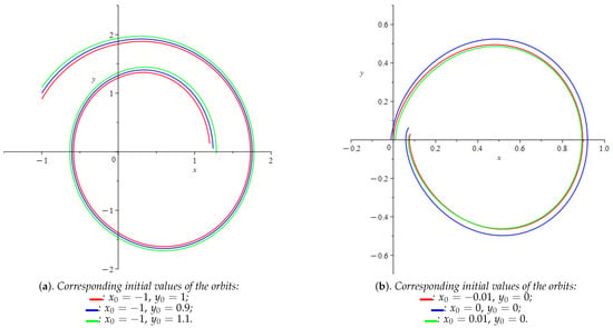
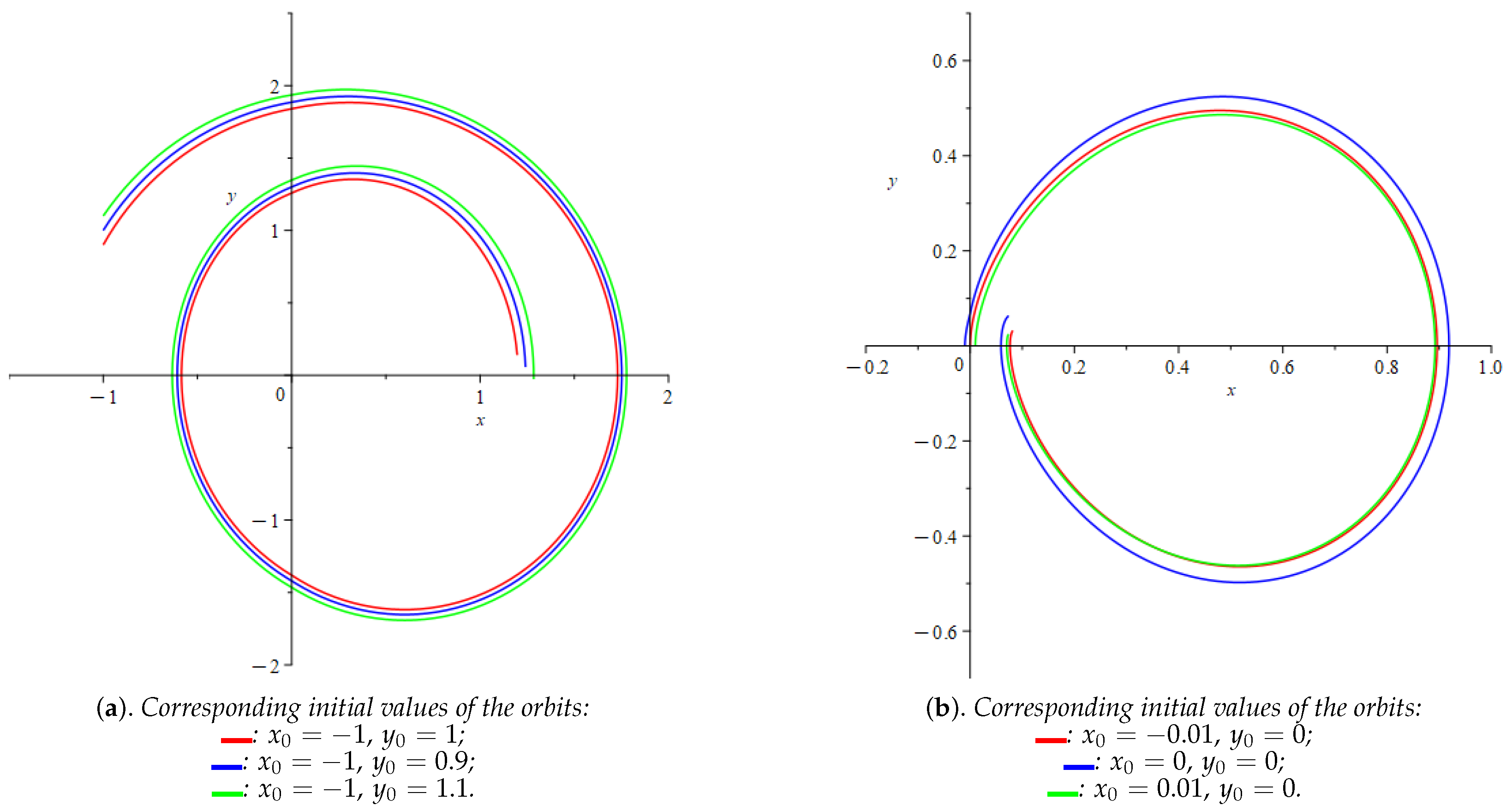
We could further verify Lemma 1 using Maple 2025. For given initial conditions $x\left(0\right)=x_0$ and $y\left(0\right)=y_0$, the orbits $P(x_0,y_0;0,2\pi )$ are illustrated in Figure 8a,b. As shown in the figures, small perturbations in the initial conditions result in only minor deviations of the orbits, which visually confirms the continuity of the Poincaré map and aligns perfectly with the statement of Lemma 1.

Compute the ratio

$${\displaystyle \frac{g_{+}\left(x\right)}{x}}={\displaystyle \frac{2x-0.2}{x}}=2-{\displaystyle \frac{0.2}{x}}.$$

Choose $A_1=1$. Then for all $x\ge 1$,

$$1.8\le 2-{\displaystyle \frac{0.2}{x}}\le 2.1.$$

Thus we can take $q_2=1.8$ and $p_2=2.1$. Compute the ratio

$${\displaystyle \frac{g_{-}\left(x\right)}{x}}={\displaystyle \frac{2x-0.1}{x}}=2-{\displaystyle \frac{0.1}{x}}.$$

Choose $A_1=1$. Then for all $x\le -1$,

$$1.9\le 2-{\displaystyle \frac{0.1}{x}}\le 2.1.$$

Thus we can take $q_1=1.9$ and $p_1=2.1$. In conclusion, by choosing $A_1=1$, $p_1=2.1$, $q_1=1.9$, $p_2=2.1$, $q_2=1.8$, the condition $\left(H_0\right)$ is satisfied.

Furthermore, we verify the condition $\left(H_2\right)$. Recall that we have chosen

$$A_1=1,p_1=2.1,q_1=1.9,p_2=2.1,q_2=1.8$$

and the discontinuous nonlinearity

$$g_{\pm }\left(x\right)=\left\{\begin{array}{c}2x-0.2,x>0,\hfill \\ 2x-0.1,x<0.\hfill \end{array}\right.$$

Substitute $p_2=2.1$ and $q_2=1.8$:

$$g_{+}\left(x\right)-p_{2}x=(2x-0.2)-2.1x=-0.1x-0.2,$$

$$g_{+}\left(x\right)-q_{2}x=(2x-0.2)-1.8x=0.2x-0.2.$$

For sufficiently large $A_2>0$ and any fixed $B>0$, when $x>A_2$,

$$g_{+}\left(x\right)-p_{2}x=-0.1x-0.2\le -B,g_{+}\left(x\right)-q_{2}x=0.2x-0.2\ge B.$$

Substitute $p_1=2.1$ and $q_1=1.9$:

$$g_{-}\left(x\right)-p_{1}x=(2x-0.1)-2.1x=-0.1x-0.1,$$

$$g_{-}\left(x\right)-q_{1}x=(2x-0.1)-1.9x=0.1x-0.1.$$

When $x<-A_2$, we have

$$g_{-}\left(x\right)-p_{1}x=-0.1x-0.1\ge B,g_{-}\left(x\right)-q_{1}x=0.1x-0.1\le -B.$$

Since $B_0$ is a fixed positive constant, we can choose $B>B_0$ and a sufficiently large $A_2>0$ such that all inequalities in $\left(H_2\right)$ hold. Therefore, the condition $\left(H_2\right)$ is satisfied.

Besides, by taking $m=1$, we obtain

$$1={\displaystyle \frac{2}{m+1}}<{\displaystyle \frac{1}{\sqrt{2.1}}}+{\displaystyle \frac{1}{\sqrt{2.1}}}\le {\displaystyle \frac{1}{\sqrt{1.8}}}+{\displaystyle \frac{1}{\sqrt{1.9}}}<{\displaystyle \frac{2}{m}}=2,$$

which satisfies the condition $\left(H_1^{\prime }\right)$ required by Theorem 3. Therefore, we conclude that the above Duffing equation admits at least one $2\pi$ crossing periodic solution.

5. Discussion

This paper investigates the existence of $2\pi$ crossing periodic solutions for a class of second-order undamped Duffing equations with discontinuity. By using the Poincaré–Bohl theorem, we obtain several existence criteria of periodic solutions.

Our core main results (Theorems 2–5) are generalized extensions of classical periodic solution theorems for continuous Duffing equations in references [1,4]. When the discontinuous nonlinearity satisfies $g_{-}\left(x\right)=g_{+}\left(x\right)$, the piecewise jump vanishes and our assumptions exactly degenerate into the original continuous growth conditions, which directly yields the corresponding classical periodic solution existence results. From this perspective, all conclusions of our paper are natural extensions of classical continuous Duffing theory to discontinuous dynamical situations, instead of isolated irrelevant findings.

The main results extend the classical theory of Duffing equations to the discontinuous case, which widely appear in practical dynamical systems including impact oscillators, mechanical structures with dry friction, and nonlinear circuits with piecewise characteristics etc.

Compared with the existing literature, the key contribution of this work is to deal with the discontinuity of the nonlinear term $g\left(x\right)$ at $x=0$, while most classical results require $g\left(x\right)$ to be continuous. By employing the Filippov theory, we establish the continuity of the Poincaré map across the discontinuity line ${\Sigma }_0$. This ensures that the Poincaré–Bohl theorem can be applied rigorously.

The conditions $\left(H_0\right)$–$\left(H_2\right)$, together with the lemmas, provide effective and checkable criteria to control the rotation speed of the solution trajectories. These conditions ensure that the Poincaré map satisfies the non-homothetic condition required by the Poincaré–Bohl theorem, leading to the existence of at least one $2\pi$ crossing periodic solution. The phase portrait analysis near the discontinuity line, combined with the estimation in polar coordinates, support the topological argument and illustrate the global dynamical behavior.

Finally, an example in Section 4 verifies that the conditions are easy to verify and can be implemented numerically. The phase diagrams generated by mathematical software show the continuity and global structure of solutions, which complement the theoretical analysis and contribute to understanding the dynamics of non-autonomous discontinuous Duffing systems.

It is worth noting that we first derive Theorem 2 under relatively strong growth restrictions on $g_{\pm }\left(x\right)$, and then gradually relax the limiting assumptions to establish Theorems 3–5 with weaker constraints. Starting from a strict and concrete setting helps us clearly uncover the intrinsic dynamical mechanism for the emergence of crossing periodic solutions in discontinuous Duffing systems on a rigorous theoretical foundation. If we directly adopt the weakest available assumptions from the outset, core dynamic rules would be concealed, and the subsequent mathematical derivation would become excessively abstract and cumbersome. Stepwise relaxation of constraints effectively broadens the applicable scope of our derived existence conclusions.

Restricted by the selected mathematical tool, this paper only proves the existence of at least one crossing periodic solution rather than uniqueness or multiplicity results. The Poincaré–Bohl fixed-point theorem used herein is merely capable of guaranteeing the existence of fixed points of the Poincaré map without counting the fixed-point quantity; unlike topological degree theory or variational approaches, it cannot characterize the number of periodic solutions. Besides, our proposed hypotheses $\left(G_1\right)$–$\left(H_2\right)$ are only formulated to verify the prerequisite of Poincaré–Bohl theorem, insufficient to add extra limitations for unique/multiple periodic solutions. Accordingly, the uniqueness, multiplicity, orbital stability and bifurcation problems of periodic solutions are reserved as promising directions for our follow-up in-depth investigation.

From the mathematical perspective, the extension of classical continuous Duffing theories to discontinuous scenarios remains incomplete. Some existing relevant researches employ implicit bounding constraints that pose challenges for practical verification, while only a modest body of literature develops explicit and readily checkable sufficient conditions for crossing periodic solutions of discontinuous non-autonomous Duffing equations. The inherent discontinuity at $x=0$ breaks the traditional continuous solution regularity, bringing extra difficulty in verifying Poincaré map continuity which classical continuous-based theories cannot resolve directly. Our work fills this literature gap by combining Filippov discontinuous differential equation theory with Poincaré mapping technique to overcome the obstacle induced by jump discontinuity, supplying an operable judgment standard for symmetric discontinuous Duffing periodic problems. Such analytical ideas can also be extended to other piecewise smooth oscillation systems in related mathematical physics fields.

6. Conclusions

This section summarizes the core content of the present paper and collects all future research suggestions as requested by the reviewer.

In this work, we focus on a class of undamped Duffing equations with state discontinuity at $x=0$ and study the existence of $2\pi$ crossing periodic solutions. Relying on Filippov regularization theory for discontinuous differential equations and the Poincaré–Bohl fixed-point theorem, we derive verifiable sufficient criteria listed in Theorems 2–5.

The key technical novelty of this paper lies in overcoming the obstacle induced by the jump discontinuity of restoring function $g\left(x\right)$. We prove the continuity of the Poincaré map crossing the discontinuity boundary ${\Sigma }_0$ under assumption $\left(G_2\right)$, which excludes sliding solutions on the discontinuous line and guarantees the rigorous applicability of the Poincaré–Bohl theorem. The numerical example in Section 4 further validates the computability and practical effectiveness of our derived theorems via phase-plane numerical simulation.

Based on the above research findings, several valuable directions for follow-up research are summarized as follows

1.

Extend the existence results to the discontinuous damped Duffing equations and explore the influence of damping on periodic solutions.

2.

Study the multiplicity, stability and bifurcation of periodic solutions for discontinuous Duffing equations.

3.

Generalize the approach to systems with multiple discontinuity points or higher-dimensional discontinuous systems.

4.

Develop more efficient numerical methods for computing periodic solutions and simulating phase portraits of discontinuous Duffing systems.

5.

Apply the theoretical results to practical engineering models such as impact oscillators and piecewise nonlinear circuits.

References

- Ding, T.; Iannacci, R.; Zanolin, F. Existence and Multiplicity Results for Periodic Solutions of Semilinear Duffing Equations. J. Differ. Equ. 1993, 105, 364–409. [Google Scholar] [CrossRef] [Scilit]
- Ding, T.; Zanolin, F. On Periodic Solutions of Sublinear Duffing Equations. J. Math. Anal. Appl. 1991, 158, 316–332. [Google Scholar] [CrossRef] [Scilit]
- Cheng, Z.; Ren, J. Harmonic and Subharmonic Solutions for Superlinear Damped Duffing Equation. Nonlinear Anal. Real World Appl. 2013, 14, 1155–1170. [Google Scholar] [CrossRef] [Scilit]
- Wang, D. On the Existence of 2π-Periodic Solutions for the Differential Equation ẍ + g(x) = p(t). Acta Math. Sin. Chin. Ser. 1984, 1, 64–75. [Google Scholar]
- Ding, T.; Zanolin, F. Subharmonic Solutions of Second Order Nonlinear Equations a Time-Map Approach. Nonlinear Anal. Theory Methods Appl. 1993, 20, 509–532. [Google Scholar] [CrossRef] [Scilit]
- Ding, T.; Zanolin, F. Time-Maps for the Solvability of Periodically Perturbed Nonlinear Duffing Equations. Nonlinear Anal. Theory Methods Appl. 1991, 17, 635–653. [Google Scholar] [CrossRef] [Scilit]
- Ding, T. Some Fixed Point Theorems and Periodically Perturbed Non-Dissipative Systems. Chin. Ann. Math. 1981, 3, 281–300. [Google Scholar]
- Fonda, A.; Torres, P. Periodic Solutions of Discontinuous Second Order Differential Equations. The porpoising effect. Nonlinear Anal. Real World Appl. 2023, 74, 103948. [Google Scholar] [CrossRef] [Scilit]
- M-Seara, T.; Silva, L.; Villanueva, J. On the Boundedness of Solutions of a Forced Discontinuous Oscillator. J. Differ. Equ. 2024, 369, 624–658. [Google Scholar] [CrossRef] [Scilit]
- Nieto, J.; Uzal, J. Periodic Solutions of Superlinear and Sublinear State-Dependent Discontinuous Differential Equations. Topol. Methods Nonlinear Anal. 2021, 58, 79–96. [Google Scholar] [CrossRef] [Scilit]
- Wen, Q.; Ren, L.; Liu, R. Existence and Uniqueness of Periodic Solution to Second-Order Impulsive Differential Equations. Math. Methods Appl. Sci. 2023, 46, 6191–6209. [Google Scholar] [CrossRef] [Scilit]
- Chawla, R.; Seth, S.; Rounak, A.; Pakrashi, V. Higher-Order Transverse Discontinuity Mapping in Filippov Systems: Analysis and Experimental Validation using an Electronic Circuit. arXiv 2025, arXiv:2506.18379. [Google Scholar] [CrossRef] [Scilit]
- Wang, Y.; Wang, Z.; Zhang, C.; Bi, Q. Bursting Oscillations with Multiple Crossing Bifurcations in a Piecewise-Smooth System. Int. J.-Non-Linear Mech. 2025, 168, 104938. [Google Scholar] [CrossRef] [Scilit]
- Chen, H.; Xie, J. Harmonic and Subharmonic Solutions of the SD Oscillator. Nonlinear Dyn. 2016, 84, 2477–2486. [Google Scholar] [CrossRef] [Scilit]
- Chen, H.; Cao, Z.; Li, D.; Xie, J. Global Analysis on a Discontinuous Dynamical System. Int. J. Bifurc. Chaos 2017, 27, 1750078. [Google Scholar] [CrossRef] [Scilit]
- Jiang, F.; Ji, Z.; Wang, Y. Periodic Solutions of Discontinuous Damped Duffing Equations. Nonlinear Anal. Real. World Appl. 2019, 47, 484–495. [Google Scholar] [CrossRef] [Scilit]
- Jiang, F. Periodic Solutions of Discontinuous Duffing Equations. Qual. Theory Dyn. Syst. 2020, 19, 93. [Google Scholar] [CrossRef] [Scilit]
- Jiang, F. Existence and Uniqueness of Crossing Periodic Solutions of a Discontinuous Mixed-Type Duffing Equation. Electron. J. Qual. Theory Differ. Equ. 2025, 2025, 1–18. [Google Scholar] [CrossRef] [Scilit]
- Leine, R.; Van Campen, D.; Van De Vrande, B. Bifurcations in Nonlinear Discontinuous Systems. Nonlinear Dyn. 2000, 23, 105–164. [Google Scholar] [CrossRef] [Scilit]
- Guo, S.; Luo, A. On Existence and Bifurcations of Periodic Motions in Discontinuous Dynamical Systems. Int. J. Bifurc. Chaos 2021, 31, 2150053. [Google Scholar] [CrossRef] [Scilit]
- Lai, C.; Chen, Y. On the Computation of Floquet Multipliers for Periodic Solution in Piecewise-smooth Dynamical System. J. Phys. Conf. Ser. 2024, 2747, 012005. [Google Scholar] [CrossRef] [Scilit]
- Niu, Y.; Li, X. Periodic Solutions of Semilinear Duffing Equations with Impulsive Effects. J. Math. Anal. Appl. 2018, 467, 349–370. [Google Scholar] [CrossRef] [Scilit]
- Jiang, F. Existence and Uniqueness of Discontinuous Periodic Orbits in Second Order Differential Equations with State-Dependent Impulses. J. Appl. Anal. Comput. 2022, 12, 69–86. [Google Scholar] [CrossRef] [Scilit] [PubMed]
- Freire, E.; Ponce, E.; Torres, F. Canonical Discontinuous Planar Piecewise Linear Systems. SIAM J. Appl. Dyn. Syst. 2012, 11, 181–211. [Google Scholar] [CrossRef] [Scilit]
- Zhou, B.; Chen, H.; Xu, H.; Zhang, J. Harmonic Solutions for a Class of Non-Autonomous Piecewise Linear Oscillators. Commun. Nonlinear Sci. Numer. Simul. 2021, 102, 105912. [Google Scholar] [CrossRef] [Scilit]
- Jia, M.; Su, Y.; Chen, H. Global Studies on a Continuous Planar Piecewise Linear Differential System with Three Zones. Nonlinear Dyn. 2023, 111, 3539–3573. [Google Scholar] [CrossRef] [Scilit]
- Hartman, P. Ordinary Differential Equations; SIAM: Philadelphia, PA, USA, 1982; Volume 38. [Google Scholar]
Disclaimer/Publisher’s Note: The statements, opinions and data contained in all publications are solely those of the individual author(s) and contributor(s) and not of MDPI and/or the editor(s). MDPI and/or the editor(s) disclaim responsibility for any injury to people or property resulting from any ideas, methods, instructions or products referred to in the content. |
© 2026 by the authors. Licensee MDPI, Basel, Switzerland. This article is an open access article distributed under the terms and conditions of the Creative Commons Attribution (CC BY) license.