A Discrete Diffusion Carbon Model: Stability, Bifurcation Analysis and Machine Learning Approach

Abstract

This paper investigates a discrete diffusion carbon emission-absorption model with periodic boundary conditions derived via the piecewise constant argument scheme. The existence of equilibrium points is established, and sufficient conditions for the local asymptotic stability of the positive equilibrium are derived through eigenvalue analysis. Then, uniform boundedness of positive solutions is proved, and the global asymptotic stability of the interior equilibrium is established by an iterative method and the comparison principle for difference equations. Furthermore, the model is shown to undergo a flip bifurcation when a critical parameter threshold is reached, leading to period-doubling dynamics and chaotic behavior. The influence of spatial diffusion is examined through a Turing instability analysis, yielding conditions for diffusion-driven instability and spatial pattern formation. Finally, Decision Tree and Random Forest classifiers are used as proof-of-concept tools to efficiently approximate the analytically derived stability regions using Monte Carlo-generated data. Both classifiers successfully reproduce the analytical stability structure, while the Random Forest classifier provides higher accuracy and smoother stability boundaries. Numerical simulations support the theoretical results and illustrate the stability and bifurcation phenomena exhibited by the model. These findings indicate that the proposed framework is useful for analyzing carbon emission-absorption dynamics and that machine learning can serve as an efficient computational surrogate for identifying stability regions in nonlinear dynamical systems.

1. Introduction

Climate change and global warming, primarily driven by the rapid increase in carbon emissions, have become among the most critical challenges of the modern world. The imbalance between carbon emission and carbon absorption processes leads to severe environmental consequences, including rising global temperatures, ecosystem degradation, and atmospheric instability. Therefore, understanding the dynamical interaction between emission and absorption mechanisms is essential for analyzing the long-term behavior of carbon systems and developing effective strategies for environmental sustainability.

In realistic environments, carbon processes are not only time-dependent but also spatially distributed. Diffusion mechanisms arising from atmospheric transport and spatial heterogeneity significantly influence the distribution of carbon concentration. To capture these effects, reaction–diffusion models have been widely used in the literature [1,2] and have provided an effective framework for investigating the interaction between local carbon dynamics and spatial transport processes.

Mathematical modeling provides a powerful framework for investigating such complex interactions [3,4]. In recent years, carbon emission-absorption systems have been modeled using nonlinear differential equations, often incorporating additional factors such as economic development, policy constraints, or external forcing. For instance, reaction-diffusion carbon models have been proposed to investigate the combined effects of spatial diffusion and economic factors on carbon dynamics; see [5]. However, the inclusion of multiple external factors may obscure the intrinsic structure of the system and complicate the analysis. Motivated by this limitation, it is essential to first understand the fundamental interaction between carbon emission and absorption mechanisms in a simplified setting.

While continuous-time models provide valuable theoretical insight, discrete-time formulations are often more appropriate in many real-world applications. Carbon-related processes are frequently observed at discrete time intervals, and environmental policies are commonly implemented periodically. Furthermore, discrete systems can exhibit richer dynamical behaviors than their continuous counterparts, including stability switches, bifurcations, and complex oscillatory patterns. These properties make discrete-time models particularly suitable for describing realistic carbon dynamics.

Most of the comprehensive studies in the dynamical systems literature primarily consider analytical approaches, including local stability, global stability, and bifurcation analysis, to examine the dynamics of nonlinear systems [6,7,8,9]. Nevertheless, determining stability regions in multidimensional parameter spaces remains a challenging task. Recently, machine learning (ML) methods have emerged as efficient tools for approximating complex nonlinear relationships and identifying stability boundaries. In particular, classification-based approaches such as Decision Trees and Random Forests have been successfully used in [10,11] to approximate analytically derived stability regions in discrete dynamical systems. These approaches act as computational surrogates that significantly reduce analytical complexity while maintaining accuracy.

Despite recent advances in combining nonlinear dynamical analysis and machine learning techniques, existing studies have focused predominantly on ecological and predator-prey systems. The present work differs in several important respects. First, it develops a discrete carbon emission-absorption model derived systematically from a continuous reaction-diffusion framework via the piecewise constant argument approach. Second, beyond local stability and bifurcation analysis, the global asymptotic stability of the positive equilibrium is established rigorously. Third, diffusion-driven Turing instability is investigated in the corresponding discrete spatial model. Finally, machine learning is employed as a computational surrogate to approximate analytically derived stability regions in a high-dimensional parameter space. Together, these components provide a unified framework that distinguishes the present study from existing machine-learning-assisted bifurcation analyses. Moreover, global stability results for discrete spatiotemporal carbon models of this type are still very limited in the literature, making the analysis both theoretically and environmentally significant.

Based on these considerations, we investigate a carbon emission–absorption framework that captures the fundamental interaction between emission and absorption processes. Emission sources increase carbon concentration locally, while absorption mechanisms such as vegetation and oceans reduce it, creating a spatially distributed interaction. Incorporating diffusion into the model allows for a more accurate representation of these processes and enables the investigation of spatial dynamics, including pattern formation and diffusion-driven instability mechanisms. To account for these effects, we begin with the following reaction–diffusion model of carbon emission and absorption in continuous space and time:

$$\begin{array}{c}\hfill {\displaystyle \frac{\partial u}{\partial t}}=d_1{\displaystyle \frac{{\partial }^{2}u}{\partial x^2}}+r_{1}u\left(1-{\displaystyle \frac{u}{n_1}}-s_1{\displaystyle \frac{v}{n_2}}\right),\\ \hfill {\displaystyle \frac{\partial v}{\partial t}}=d_2{\displaystyle \frac{{\partial }^{2}v}{\partial x^2}}+r_{2}v\left(1-{\displaystyle \frac{v}{n_2}}-s_2{\displaystyle \frac{u}{n_1}}\right),\end{array}$$

(1)

where $x\in \mathsf{\Omega }=[0,\pi ]$, the domain $\mathsf{\Omega }$ has a smooth boundary $\partial \mathsf{\Omega }$, and time $t\ge 0$. The state variables $u(x,t)$ and $v(x,t)$ denote the densities of carbon emission and carbon absorption at position x and time t, respectively. The parameters $d_1$ and $d_2$ represent the diffusion coefficients of carbon dioxide at high and low concentrations, respectively. The parameters $r_1$ and $r_2$ denote the average growth rates of carbon emission and carbon absorption, respectively. The constants $n_1$ and $n_2$ represent the maximum carbon density that the environment can accommodate and the maximum carbon absorption capacity per unit area, respectively. The dimensionless parameters $s_1$ and $s_2$ describe the mutual influence between carbon emission and carbon absorption processes.

To analyze carbon emission and absorption dynamics under the influence of external factors, particularly economic development, we consider the reaction-diffusion dual carbon model introduced in [5]. In that framework, economic development is incorporated as a dominant factor affecting carbon emission behavior. In contrast, the present study focuses on the intrinsic structure of the carbon emission-absorption interaction by formulating the model without the inclusion of external driving factors. By removing the economic component, the model is restructured to capture the fundamental nonlinear interaction between emission and absorption processes. This approach enables a clearer investigation of the inherent dynamical properties of the carbon system and provides a more transparent framework for analyzing its stability behavior. In the present study, the logistic growth structure is adopted as a phenomenological approximation for the long-term evolution of carbon emissions. Although carbon emissions are primarily driven by industrial activity, energy consumption, and economic development rather than biological processes, unrestricted exponential growth is unlikely to persist over long time horizons. In practice, emission growth is constrained by finite resources, technological saturation, environmental regulations, decarbonization policies, and broader socio-economic adaptation mechanisms. These combined effects can be represented mathematically through a carrying-capacity-type mechanism, leading naturally to a logistic formulation. Accordingly, the logistic term should be interpreted as an effective nonlinear representation of bounded growth dynamics.

Continuous-time model (1) provides valuable insight into the mechanisms governing carbon emission-absorption interactions. However, in practice, carbon-related processes are often observed, regulated, and controlled in a discrete manner, for example through periodic measurements, seasonal effects, or stepwise policy interventions. Therefore, a discrete-time formulation is more appropriate for capturing the observed dynamics and may reveal richer dynamical behaviors than its continuous counterpart. Applying a piecewise constant parameter method based on differential equations to system (1), we obtain the following discrete-time carbon emission-absorption model:

$$\left\{\begin{array}{c}{u}_{t+1}=u_{t}exp\left[r_1\left(1-{\displaystyle \frac{u_t}{n_1}}-{\displaystyle \frac{s_1{v}_t}{n_2}}\right)\right],\hfill \\ v_{t+1}=v_{t}exp\left[r_2\left(1-{\displaystyle \frac{v_t}{n_2}}-{\displaystyle \frac{s_2{u}_t}{n_1}}\right)\right],\hfill \end{array}\right.$$

(2)

It is straightforward to verify that if $u_0>0$ and $v_0>0$, then the solutions of (2) remain positive for all $t\ge 0$.

To model the spatial structure, we consider a two-dimensional discrete domain consisting of an $n\times n$ lattice. Each lattice point represents a spatial location, and two state variables are assigned to each site. Let $u_t^{i,j}$ and $v_t^{i,j}$ denote the carbon emission density and carbon absorption density at location $(i,j)$ and time t, respectively, where $(i,j)\in {\{1,2,\dots ,n\}}^2$ and $t\in {\mathbb{Z}}^{+}$.

By incorporating the diffusion mechanism into model (2), the system is extended to a space-time discrete framework. In this formulation, the local dynamics given by the reaction terms are combined with spatial interactions represented by the discrete Laplacian operator. Consequently, model (2) is transformed into the following form:

$$\left\{\begin{array}{c}{u}_{t+1}^{i,j}=u_t^{i,j}exp\left[r_1\left(1-{\displaystyle \frac{u_t^{i,j}}{n_1}}-{\displaystyle \frac{s_1{v}_t^{i,j}}{n_2}}\right)\right]+d_1{\nabla }^2{u}_t^{i,j},\hfill \\ v_{t+1}^{i,j}=v_t^{i,j}exp\left[r_2\left(1-{\displaystyle \frac{v_t^{i,j}}{n_2}}-{\displaystyle \frac{s_2{u}_t^{i,j}}{n_1}}\right)\right]+d_2{\nabla }^2{v}_t^{i,j},\hfill \end{array}\right.$$

(3)

with the periodic boundary conditions

$$u_t^{i,0}=u_t^{i,n},u_t^{i,1}=u_t^{i,n+1},$$

$$v_t^{i,0}=v_t^{i,n},v_t^{i,1}=v_t^{i,n+1},$$

$$u_t^{0,j}=u_t^{n,j},u_t^{1,j}=u_t^{n+1,j},$$

$$v_t^{0,j}=v_t^{n,j},v_t^{1,j}=v_t^{n+1,j}.$$

$d_1$ and $d_2$ are diffusion parameters.

$${\nabla }^2{u}_t^{ij}=u_t^{i+1,j}+u_t^{i,j+1}+u_t^{i-1,j}+u_t^{i,j-1}-4u_t^{ij},$$

$${\nabla }^2{v}_t^{ij}=v_t^{i+1,j}+v_t^{i,j+1}+v_t^{i-1,j}+v_t^{i,j-1}-4v_t^{ij}.$$

where ${\nabla }^2$ denotes the discrete Laplacian operator and periodic boundary conditions are imposed.

The structure of this paper is organized as follows for discussion. In Section 2, we systematically analyze the dynamic characteristics of model (2), exploring the local and global stability of the positive equilibrium point and the uniform boundedness of solutions, to comprehensively understand the dynamic behavior of the system. It is shown that the sufficient criterion for flip bifurcation can be established. Section 3 investigates the effects of spatial diffusion and establishes the conditions under which Turing instability occurs in the discrete carbon emission–absorption model. Subsequently, in Section 4, we examine stability transitions and employ machine learning techniques to classify stability regions. Finally, in Section 5, we summarize the research content and findings of the paper, providing an in-depth interpretation and discussion of the results obtained.

2. Dynamical Analysis of the Discrete Carbon Model

In order to ensure the existence and uniqueness of solutions of model (2), we consider initial conditions $(u_0,v_0)\in {\mathbb{R}}_{+}^2=\{(u,v):u>0,v>0\}$, where all standard assumptions for well-posedness are satisfied.

Theorem 1.

1. 

Model (2) always has a trivial equilibrium point $E_0(0,0)$.

2. 

Model (2) has two boundary equilibrium points $E_1(n_1,0)$ and $E_2(0,n_2)$.

3. 

If $1-s_1>0$, $1-s_2>0$, and $1-s_1{s}_2>0$, then model (2) has a unique positive interior equilibrium point $E^{*}(u^{*},v^{*})$, where

$$u^{*}={\displaystyle \frac{n_1(1-s_1)}{1-s_1{s}_2}},v^{*}={\displaystyle \frac{n_2(1-s_2)}{1-s_1{s}_2}}.$$

In this case, both components of the system coexist.

Proof. 

The equilibrium points of model (2) satisfy the following system:

$$\left\{\begin{array}{c}u=uexp\left[r_1\left(1-{\displaystyle \frac{u}{n_1}}-{\displaystyle \frac{s_{1}v}{n_2}}\right)\right],\hfill \\ v=vexp\left[r_2\left(1-{\displaystyle \frac{v}{n_2}}-{\displaystyle \frac{s_{2}u}{n_1}}\right)\right].\hfill \end{array}\right.$$

Clearly, $E_0=(0,0)$ is an equilibrium point.

If $v=0$ and $u>0$, then

$$1-{\displaystyle \frac{u}{n_1}}=0,$$

which gives $u=n_1$. Hence, $E_1=(n_1,0)$ is a boundary equilibrium point.

Similarly, if $u=0$ and $v>0$, then

$$1-{\displaystyle \frac{v}{n_2}}=0,$$

which gives $v=n_2$. Thus, $E_2=(0,n_2)$ is another boundary equilibrium point.

Now assume that $u>0$ and $v>0$. Then the system reduces to

$$1-{\displaystyle \frac{u}{n_1}}-{\displaystyle \frac{s_{1}v}{n_2}}=0,1-{\displaystyle \frac{v}{n_2}}-{\displaystyle \frac{s_{2}u}{n_1}}=0.$$

Solving this linear system yields

$$u^{*}={\displaystyle \frac{n_1(1-s_1)}{1-s_1{s}_2}},v^{*}={\displaystyle \frac{n_2(1-s_2)}{1-s_1{s}_2}}.$$

Therefore, the positive equilibrium exists if and only if

$$u^{*}>0,v^{*}>0,$$

which holds under the conditions $1-s_1>0$, $1-s_2>0$, and $1-s_1{s}_2>0$. This completes the proof. □

The linearized form of model (2) about an arbitrary equilibrium point $E(u,v)\in {\mathbb{R}}_{+}^2$ under the map

$$(f,g)⟼(u_{t+1},v_{t+1})$$

is given by

$${\mathsf{\Phi }}_{t+1}{=J|}_E{\mathsf{\Phi }}_t,$$

where

$${\mathsf{\Phi }}_t=\left(\begin{array}{c}{u}_t\\ v_t\end{array}\right){,J|}_E={\left(\begin{array}{cc}{f}_u& f_v\\ g_u& g_v\end{array}\right)}_{(u,v)}.$$

To study the local stability of the equilibrium points, we derive the Jacobian matrix ${J|}_E$ of model (2), given by

$${J|}_E=\left(\begin{array}{cc}\left(1-{\displaystyle \frac{r_{1}u}{n_1}}\right)exp\left[r_1\left(1-{\displaystyle \frac{u}{n_1}}-{\displaystyle \frac{s_{1}v}{n_2}}\right)\right]& -{\displaystyle \frac{r_1{s}_{1}u}{n_2}}exp\left[r_1\left(1-{\displaystyle \frac{u}{n_1}}-{\displaystyle \frac{s_{1}v}{n_2}}\right)\right]\\ -{\displaystyle \frac{r_2{s}_{2}v}{n_1}}exp\left[r_2\left(1-{\displaystyle \frac{v}{n_2}}-{\displaystyle \frac{s_{2}u}{n_1}}\right)\right]& \left(1-{\displaystyle \frac{r_{2}v}{n_2}}\right)exp\left[r_2\left(1-{\displaystyle \frac{v}{n_2}}-{\displaystyle \frac{s_{2}u}{n_1}}\right)\right]\end{array}\right).$$

Theorem 2.

The trivial equilibrium point $E_0$ of model (2) is a source point, and hence it is unstable.

Proof. 

For the equilibrium point $E_0(0,0)$, we have

$${J|}_{E_0}=\left(\begin{array}{cc}{e}^{r_1}& 0\\ 0& e^{r_2}\end{array}\right).$$

The eigenvalues of ${J|}_{E_0}$ are

$${\lambda }_1=e^{r_1},{\lambda }_2=e^{r_2}.$$

Since $r_1>0$ and $r_2>0$, we obtain

$$|{\lambda }_1|=e^{r_1}>1,\left|{\lambda }_2\right|=e^{r_2}>1.$$

Therefore, both eigenvalues lie outside the unit circle. Hence, $E_0$ is a source, and consequently it is unstable. □

For the boundary equilibrium point $E_1(n_1,0)$, we have

$${J|}_{E_1}=\left(\begin{array}{cc}1-r_1& -{\displaystyle \frac{r_1{s}_1{n}_1}{n_2}}\\ 0& e^{r_2(1-s_2)}\end{array}\right).$$

The eigenvalues of ${J|}_{E_1}$ are

$${\lambda }_1=1-r_1,{\lambda }_2=e^{r_2(1-s_2)}.$$

The properties of the boundary equilibrium point $E_1(n_1,0)$ are summarized in Table 1.

Table 1. Properties of equilibrium point $E_1(n_1,0)$.

Conditions	${\mathit{\lambda }}_1=1-{\mathit{r}}_1$	${\mathit{\lambda }}_2={\mathit{e}}^{{\mathit{r}}_2(1-{\mathit{s}}_2)}$	Properties
$0<r_1<2$	$|{\lambda }_1|<1$	$s_2>1,\left|{\lambda }_2\right|<1$	Sink
		$s_2<1,\left|{\lambda }_2\right|>1$	Saddle
		$s_2=1,\left|{\lambda }_2\right|=1$	Non-hyperbolic
$r_1>2$	$|{\lambda }_1|>1$	$s_2>1,\left|{\lambda }_2\right|<1$	Saddle
		$s_2<1,\left|{\lambda }_2\right|>1$	Source
		$s_2=1,\left|{\lambda }_2\right|=1$	Non-hyperbolic
$r_1=2$	$|{\lambda }_1|=1$	$s_2>1,\left|{\lambda }_2\right|<1$	Non-hyperbolic
		$s_2<1,\left|{\lambda }_2\right|>1$	Non-hyperbolic
		$s_2=1,\left|{\lambda }_2\right|=1$	Non-hyperbolic

For the boundary equilibrium point $E_2(0,n_2)$, we have

$${J|}_{E_2}=\left(\begin{array}{cc}{e}^{r_1(1-s_1)}& 0\\ -{\displaystyle \frac{r_2{s}_2{n}_2}{n_1}}& 1-r_2\end{array}\right).$$

The eigenvalues of ${J|}_{E_2}$ are

$${\lambda }_1=e^{r_1(1-s_1)},{\lambda }_2=1-r_2.$$

The properties of the boundary equilibrium point $E_2(0,n_2)$ are summarized in Table 2.

Table 2. Properties of equilibrium point $E_2(0,n_2)$.

Conditions	${\mathit{\lambda }}_1={\mathit{e}}^{{\mathit{r}}_1(1-{\mathit{s}}_1)}$	${\mathit{\lambda }}_2=1-{\mathit{r}}_2$	Properties
$0<r_2<2$	$|{\lambda }_2|<1$	$s_1>1,\left|{\lambda }_1\right|<1$	Sink
		$s_1<1,\left|{\lambda }_1\right|>1$	Saddle
		$s_1=1,\left|{\lambda }_1\right|=1$	Non-hyperbolic
$r_2>2$	$|{\lambda }_2|>1$	$s_1>1,\left|{\lambda }_1\right|<1$	Saddle
		$s_1<1,\left|{\lambda }_1\right|>1$	Source
		$s_1=1,\left|{\lambda }_1\right|=1$	Non-hyperbolic
$r_2=2$	$|{\lambda }_2|=1$	$s_1>1,\left|{\lambda }_1\right|<1$	Non-hyperbolic
		$s_1<1,\left|{\lambda }_1\right|>1$	Non-hyperbolic
		$s_1=1,\left|{\lambda }_1\right|=1$	Non-hyperbolic

According to Table 1 and Table 2, the following results can be obtained.

Theorem 3.

The boundary equilibrium point $E_1(n_1,0)$ is locally asymptotically stable if

$$0<r_1<2\mathrm{and}{s}_2>1.$$

Theorem 4.

The boundary equilibrium point $E_2(0,n_2)$ is locally asymptotically stable if

$$0<r_2<2\mathrm{and}{s}_1>1.$$

The Jacobian matrix of model (2) evaluated at the positive equilibrium point is given by

$${J|}_{E^{*}}=\left(\begin{array}{cc}1-{\displaystyle \frac{r_1(1-s_1)}{1-s_1{s}_2}}& -{\displaystyle \frac{r_1{s}_1{n}_1(1-s_1)}{n_2(1-s_1{s}_2)}}\\ -{\displaystyle \frac{r_2{s}_2{n}_2(1-s_2)}{n_1(1-s_1{s}_2)}}& 1-{\displaystyle \frac{r_2(1-s_2)}{1-s_1{s}_2}}\end{array}\right).$$

For simplicity, we introduce the following notations:

$$a_1=r_1(1-s_1),a_2=r_2(1-s_2),a_3=1-s_1{s}_2.$$

Then, the Jacobian matrix can be written as

$${J|}_{E^{*}}=\left(\begin{array}{cc}1-{\displaystyle \frac{a_1}{a_3}}& -{\displaystyle \frac{s_1{a}_1{n}_1}{n_2{a}_3}}\\ -{\displaystyle \frac{s_2{a}_2{n}_2}{n_1{a}_3}}& 1-{\displaystyle \frac{a_2}{a_3}}\end{array}\right).$$

The corresponding characteristic polynomial is given by

$$F\left(\lambda \right)={\lambda }^2-T\lambda +D,$$

where

$$T=Tr\left(J{|}_{E^{*}}\right)=2-{\displaystyle \frac{a_1+a_2}{a_3}},$$

$$D=det\left(J{|}_{E^{*}}\right)=1-{\displaystyle \frac{a_1+a_2}{a_3}}+{\displaystyle \frac{a_1{a}_2}{a_3}}.$$

Lemma 1

([12]). Suppose that

$$F\left(\lambda \right)={\lambda }^2-T\lambda +D,$$

and $F\left(1\right)>0$, where ${\lambda }_1$ and ${\lambda }_2$ are the roots of $F\left(\lambda \right)=0$. Then the following results hold:

1. 

$|{\lambda }_1|<1$ and $|{\lambda }_2|<1$ if and only if

$$F(-1)>0\mathrm{and}D<1.$$

2. 

$|{\lambda }_1|>1$ and $|{\lambda }_2|>1$ if and only if

$$F(-1)>0\mathrm{and}D>1.$$

3. 

$|{\lambda }_1|<1<|{\lambda }_2|$ or $|{\lambda }_2|<1<|{\lambda }_1|$ if and only if

$$F(-1)<0.$$

4. 

${\lambda }_1=-1$ and ${\lambda }_2\ne 1$ if and only if

$$F(-1)=0\mathrm{and}T\ne 0,2.$$

5. 

${\lambda }_1$ and ${\lambda }_2$ are complex and $|{\lambda }_1|=|{\lambda }_2|=1$ if and only if

$$T^2-4D<0\mathrm{and}D=1.$$

Theorem 5.

Assume that $E^{*}$ is the unique positive interior equilibrium point of model (2) and

$$F\left(1\right)={\displaystyle \frac{a_1{a}_2}{a_3}}>0.$$

Then the following results hold:

1. 

$E^{*}$ is a sink if and only if

$$0<{\displaystyle \frac{a_1{a}_2}{a_3}}<{\displaystyle \frac{a_1+a_2}{a_3}}$$

and

$$4-2{\displaystyle \frac{a_1+a_2}{a_3}}+{\displaystyle \frac{a_1{a}_2}{a_3}}>0.$$

2. 

$E^{*}$ is a saddle if and only if

$$4-2{\displaystyle \frac{a_1+a_2}{a_3}}+{\displaystyle \frac{a_1{a}_2}{a_3}}<0.$$

3. 

$E^{*}$ is a source if and only if

$${\displaystyle \frac{a_1{a}_2}{a_3}}>{\displaystyle \frac{a_1+a_2}{a_3}}$$

and

$$4-2{\displaystyle \frac{a_1+a_2}{a_3}}+{\displaystyle \frac{a_1{a}_2}{a_3}}>0.$$

4. 

$E^{*}$ is non-hyperbolic if one of the following holds:

$$4-2{\displaystyle \frac{a_1+a_2}{a_3}}+{\displaystyle \frac{a_1{a}_2}{a_3}}=0,2-{\displaystyle \frac{a_1+a_2}{a_3}}\ne 0,2,$$

or

$${\displaystyle \frac{a_1{a}_2}{a_3}}={\displaystyle \frac{a_1+a_2}{a_3}},$$

$${(a_1+a_2)}^2-4a_1{a}_2{a}_3<0.$$

Proof. 

According to Lemma 1, the positive equilibrium point $E^{*}$ is a sink if and only if

$$F\left(1\right)>0,F(-1)>0,D<1$$

hold. Since

$$F\left(1\right)={\displaystyle \frac{a_1{a}_2}{a_3}},$$

$$F(-1)=4-2{\displaystyle \frac{a_1+a_2}{a_3}}+{\displaystyle \frac{a_1{a}_2}{a_3}},$$

and

$$D=1-{\displaystyle \frac{a_1+a_2}{a_3}}+{\displaystyle \frac{a_1{a}_2}{a_3}}.$$

These conditions imply

$$0<{\displaystyle \frac{a_1{a}_2}{a_3}}<{\displaystyle \frac{a_1+a_2}{a_3}}$$

and

$$4-2{\displaystyle \frac{a_1+a_2}{a_3}}+{\displaystyle \frac{a_1{a}_2}{a_3}}>0.$$

Thus, item (1) holds.

The same reasoning, together with the remaining parts of Lemma 1, gives items 2–4. This completes the proof. □

Theorem 6.

When the conditions

$$0<{\displaystyle \frac{a_1{a}_2}{a_3}}<{\displaystyle \frac{a_1+a_2}{a_3}}$$

and

$$4-2{\displaystyle \frac{a_1+a_2}{a_3}}+{\displaystyle \frac{a_1{a}_2}{a_3}}>0$$

are satisfied, model (2) is locally asymptotically stable at the positive equilibrium point $E^{*}$.

Proof. 

According to Lemma 1 and Theorem 5, when

$$|{\lambda }_1|<1\mathrm{and}|{\lambda }_2|<1,$$

$E^{*}$ is a sink point and locally asymptotically stable. This means that

$$0<{\displaystyle \frac{a_1{a}_2}{a_3}}<{\displaystyle \frac{a_1+a_2}{a_3}}$$

and

$$4-2{\displaystyle \frac{a_1+a_2}{a_3}}+{\displaystyle \frac{a_1{a}_2}{a_3}}>0.$$

Hence, $E^{*}$ is locally asymptotically stable. □

Lemma 2

([13]). Suppose that $\left\{u_t\right\}$ satisfies

$$u_0>0\mathrm{and}{u}_{t+1}\le u_{t}exp\left(A(1-B{u}_t)\right),t\in [0,+\infty ),$$

where A and B are positive constants. Then,

$$\underset{t\to \infty }{lim\; sup}{u}_t\le {\displaystyle \frac{1}{AB}}exp(A-1).$$

We now state the theorem which ensures that every positive solution of the system (2) is uniformly bounded.

Theorem 7.

Each positive solution $\left\{(u_t,v_t)\right\}$ of model (2) is uniformly bounded.

Proof. 

Assume that $\left\{(u_t,v_t)\right\}$ is an arbitrary solution of model (2). From the first equation of model (2), we obtain

$$u_{t+1}=u_{t}exp\left[r_1\left(1-{\displaystyle \frac{u_t}{n_1}}-{\displaystyle \frac{s_1}{n_2}}{v}_t\right)\right]\le u_{t}exp\left[r_1\left(1-{\displaystyle \frac{u_t}{n_1}}\right)\right],t=1,2,\dots$$

Assume that $u_0>0$. Then, by Lemma 2, we obtain

$$\underset{t\to \infty }{lim\; sup}{u}_t\le {\displaystyle \frac{n_1}{r_1}}exp(r_1-1)=M_1.$$

From the second equation of model (2), we have

$$v_{t+1}=v_{t}exp\left[r_2\left(1-{\displaystyle \frac{v_t}{n_2}}-{\displaystyle \frac{s_2}{n_1}}{u}_t\right)\right]\le v_{t}exp\left[r_2\left(1-{\displaystyle \frac{v_t}{n_2}}\right)\right].$$

Since $v_0>0$, by Lemma 2, we obtain

$$\underset{t\to \infty }{lim\; sup}{v}_t\le {\displaystyle \frac{n_2}{r_2}}exp(r_2-1)=:M_2.$$

Therefore,

$$\underset{t\to \infty }{lim\; sup}{u}_t\le M_1,\underset{t\to \infty }{lim\; sup}{v}_t\le M_2.$$

Let $M=max\{M_1,M_2\}$. Then

$$\underset{t\to \infty }{lim\; sup}(u_t,v_t)\le M.$$

Hence, each positive solution of model (2) is uniformly bounded. This completes the proof. □

Next, we will obtain the global asymptotically stability of the positive equilibrium point $E^{*}=(u^{*},v^{*})$ by an iterative method.

Lemma 3

([14]). Consider the function

$$f\left(u\right)=uexp(m-wu),$$

where m and w are constants. Then $f\left(u\right)$ is non-decreasing on $u\in (0,1/w]$ provided that $m\le 1$.

Lemma 4

([14]). Suppose that the sequence $\left\{u_t\right\}$ satisfies

$$u_{t+1}=u_{t}exp(m-w{u}_t),t\in \mathbb{N},$$

where m and w are non-negative constants and $u_0>0$. Then the following results hold:

(a) 

If $m<2$, then

$$\underset{t\to +\infty }{lim}{u}_t={\displaystyle \frac{m}{w}}.$$

(b) 

If $m\le 1$, then

$$u_t\le {\displaystyle \frac{1}{w}},\mathrm{for}\mathrm{all}t\in \mathbb{N}.$$

Lemma 5

([14]). Assume that the functions

$$f,g:{\mathbb{Z}}^{+}\times [0,+\infty )\to [0,+\infty )$$

satisfy

$$f(t,z)\le g(t,z)\left(\mathrm{or}f\right(t,z)\ge g(t,z\left)\right)$$

for all $t\in {\mathbb{Z}}^{+}$ and $z\in [0,+\infty )$, and that $g(t,z)$ is non-decreasing with respect to $z>0$. If the sequences $\left\{z_t\right\}$ and $\left\{y_t\right\}$ are positive solutions of the following difference equation, respectively,

$$z_{t+1}=f(t,z_t),y_{t+1}=g(t,y_t),t=0,1,2,\dots$$

with

$$z_0\le y_0(\mathrm{or}{z}_0\ge y_0),$$

then there exist

$$z_t\le y_t(\mathrm{or}{z}_t\ge y_t)\mathrm{for}\mathrm{all}t=0,1,2,\dots$$

Theorem 8.

Assume that the positive interior equilibrium point $E^{*}=(u^{*},v^{*})$ exists, where

$$u^{*}={\displaystyle \frac{n_1(1-s_1)}{1-s_1{s}_2}},v^{*}={\displaystyle \frac{n_2(1-s_2)}{1-s_1{s}_2}}.$$

Let $s_1,s_2\in (0,1)$ and $s_1{s}_2<1$. The interior equilibrium point $E^{*}=(u^{*},v^{*})$ is globally asymptotically stable if the following conditions are satisfied:

$$0<{\displaystyle \frac{r_1}{n_1}}{N}_3^u<{\displaystyle \frac{r_1}{n_1}}{M}_3^u\le 1,0<{\displaystyle \frac{r_2}{n_2}}{N}_4^v<{\displaystyle \frac{r_2}{n_2}}{M}_4^v\le 1,$$

where

$$M_3^u=n_1,M_4^v=n_2,$$

and

$$N_3^u=n_1\left(1-{\displaystyle \frac{s_1}{n_2}}{M}_4^v\right),N_4^v=n_2\left(1-{\displaystyle \frac{s_2}{n_1}}{M}_3^u\right).$$

Proof. 

Suppose that $(u_t,v_t)$ is an arbitrary positive solution corresponding to model (2) with the initial values $u_0,v_0>0$. Define

$$M_3=\underset{t\to \infty }{lim\; sup}{u}_t,M_4=\underset{t\to \infty }{lim\; sup}{v}_t,$$

and

$$N_3=\underset{t\to \infty }{lim\; inf}{u}_t,N_4=\underset{t\to \infty }{lim\; inf}{v}_t.$$

Next, we prove the global asymptotic stability of the positive equilibrium point $E^{*}=(u^{*},v^{*})$ by an iterative method. □

Iteration 1. The goal is to prove that $M_3\le M_3^u$ and $M_4\le M_4^v$. From the first part of model (2), we have

$$\begin{array}{cc}\hfill u_{t+1}& =u_{t}exp\left[r_1\left(1-{\displaystyle \frac{u_t}{n_1}}-{\displaystyle \frac{s_1{v}_t}{n_2}}\right)\right]\hfill \\ & \le u_{t}exp\left[r_1\left(1-{\displaystyle \frac{u_t}{n_1}}\right)\right].\hfill \end{array}$$

Consider the auxiliary equation

$$z_{t+1}=z_{t}exp\left[r_1-{\displaystyle \frac{r_1}{n_1}}{z}_t\right]0<r_1\le 1$$

By part (b) of Lemma 4, we obtain

$$z_t\le {\displaystyle \frac{n_1}{r_1}},\mathrm{if}{r}_1\le 1.$$

Moreover, the function

$$f\left(z\right)=z_{t}exp\left[r_1-{\displaystyle \frac{r_1}{n_1}}{z}_t\right]$$

is non-decreasing for $z\in (0,{\displaystyle \frac{n_1}{r_1}}],$ which follows from Lemma 3. Thus, from Lemma 5, we have

$$u_t\le z_t\mathrm{for}\mathrm{all}t\ge 2.$$

So

$$\underset{t\to \infty }{lim\; sup}{u}_t\le \underset{t\to \infty }{lim}{z}_t.$$

From part (a) of Lemma 4, we have

$$\underset{t\to \infty }{lim}{z}_t=n_1.$$

Hence,

$$M_3=\underset{t\to \infty }{lim\; sup}{u}_t\le n_1=M_3^u.$$

Thus, for any sufficiently small $\epsilon >0$, there exists $t_1>2$ such that

$$u_t\le M_3^u+\epsilon ,\mathrm{for}\mathrm{all}t\ge t_1.$$

From the second part of model (2), we have

$$\begin{array}{cc}\hfill v_{t+1}& =v_{t}exp\left[r_2\left(1-{\displaystyle \frac{v_t}{n_2}}-{\displaystyle \frac{s_2}{n_1}}{u}_t\right)\right]\hfill \\ & \le v_{t}exp\left[r_2\left(1-{\displaystyle \frac{v_t}{n_2}}\right)\right].\hfill \end{array}$$

Consider the auxiliary equation

$$z_{t+1}=z_{t}exp\left[r_2-{\displaystyle \frac{r_2}{n_2}}{z}_t\right],0<r_2\le 1.$$

By part (b) of Lemma 4, we obtain

$$z_t\le {\displaystyle \frac{n_2}{r_2}},\mathrm{for}\mathrm{all}t\ge 2.$$

Moreover, the function

$$f\left(z\right)=z_{t}exp\left[r_2-{\displaystyle \frac{r_2}{n_2}}{z}_t\right]$$

is non-decreasing for $z\in \left(0,{\displaystyle \frac{n_2}{r_2}}\right],$ which follows from Lemma 3. Thus, from Lemma 5, we have

$$v_t\le z_t\mathrm{for}\mathrm{all}t\ge t_1.$$

Therefore,

$$\underset{t\to \infty }{lim\; sup}{v}_t\le \underset{t\to \infty }{lim}{z}_t.$$

From part (a) of Lemma 4, we have

$$\underset{t\to \infty }{lim}{z}_t=n_2.$$

Hence,

$$M_4=\underset{t\to \infty }{lim\; sup}{v}_t\le n_2.$$

Therefore, we define

$$M_4^v=n_2.$$

Consequently, for any sufficiently small $\epsilon >0$, there exists $t_2>t_1$ such that

$$v_t\le M_4^v+\epsilon ,\mathrm{for}\mathrm{all}t\ge t_2.$$

Iteration 2. The goal is to prove that

$$N_3\ge N_3^u,N_4\ge N_4^v.$$

From the first part of model (2), we have

$$u_{t+1}\ge u_{t}exp\left[r_1\left(1-{\displaystyle \frac{u_t}{n_1}}-{\displaystyle \frac{s_1}{n_2}}(M_4^v+\epsilon )\right)\right].$$

Combining auxiliary equation

$$z_{t+1}=z_{t}exp\left[r_1\left(1-{\displaystyle \frac{z_t}{n_1}}-{\displaystyle \frac{s_1}{n_2}}\left(M_4^v+\epsilon \right)\right)\right].$$

By part (b) of Lemma 4, we obtain

$$z_t\le {\displaystyle \frac{n_1}{r_1}},\mathrm{for}\mathrm{all}t\ge t_2.$$

Define

$$f\left(z\right)=z_{t}exp\left[r_1\left(1-{\displaystyle \frac{z_t}{n_1}}-{\displaystyle \frac{s_1}{n_2}}\left(M_4^v+\epsilon \right)\right)\right].$$

The function f is non-decreasing for $z_t\in \left(0,{\displaystyle \frac{n_1}{r_1}}\right],$ which follows from Lemma 3. Thus, from Lemma 5, we have

$$u_t\ge z_t\mathrm{for}\mathrm{all}t\ge t_2.$$

Hence,

$$\underset{t\to \infty }{lim\; inf}{u}_t\ge \underset{t\to \infty }{lim}{z}_t.$$

From part (a) of Lemma 4, we have

$$\underset{t\to \infty }{lim}{z}_t=n_1-{\displaystyle \frac{n_1{s}_1}{n_2}}\left(M_4^v+\epsilon \right).$$

Therefore,

$$N_3=\underset{t\to \infty }{lim\; inf}{u}_t\ge n_1-{\displaystyle \frac{n_1{s}_1}{n_2}}\left(M_4^v+\epsilon \right).$$

By the arbitrariness of $\epsilon >0$, we obtain

$$N_3\ge n_1-{\displaystyle \frac{n_1{s}_1}{n_2}}{M}_4^v=N_3^u.$$

Therefore, for any sufficiently small $\epsilon >0$, there exists $t_3>t_2$ such that

$$t\ge t_3\mathrm{and}{u}_t\ge N_3^u-\epsilon .$$

Similarly, from the second part of model (2), we have

$$v_{t+1}\ge v_{t}exp\left[r_2\left(1-{\displaystyle \frac{v_t}{n_2}}-{\displaystyle \frac{s_2}{n_1}}(M_3^u+\epsilon )\right)\right].$$

Combining auxiliary equation

$$z_{t+1}=z_{t}exp\left[r_2\left(1-{\displaystyle \frac{z_t}{n_2}}-{\displaystyle \frac{s_2}{n_1}}(M_3^u+\epsilon )\right)\right],$$

by part (b) of Lemma 4, we obtain

$$z_t\le {\displaystyle \frac{n_2}{r_2}},\mathrm{for}\mathrm{all}\mathrm{sufficiently}\mathrm{large}t.$$

Thus, from Lemma 5, we have

$$v_t\ge z_t,$$

and hence

$$\underset{t\to \infty }{lim\; inf}{v}_t\ge \underset{t\to \infty }{lim}{z}_t.$$

From part (a) of Lemma 4, we obtain

$$\underset{t\to \infty }{lim}{z}_t=n_2\left[1-{\displaystyle \frac{s_2}{n_1}}(M_3^u+\epsilon )\right].$$

Hence,

$$N_4=\underset{t\to \infty }{lim\; inf}{v}_t\ge n_2\left[1-{\displaystyle \frac{s_2}{n_1}}(M_3^u+\epsilon )\right].$$

By the arbitrariness of $\epsilon >0$, we have

$$N_4\ge n_2\left[1-{\displaystyle \frac{s_2}{n_1}}{M}_3^u\right]=N_4^v.$$

Iteration 3. The goal is to prove that

$$M_3\le M_5^u\mathrm{and}{M}_4\le M_6^v,$$

where

$$M_5^u\le M_3^u\mathrm{and}{M}_6^v\le M_4^v.$$

From the first part of model (2), for $t>t_4$, we have

$$u_{t+1}\le u_{t}exp\left[r_1\left(1-{\displaystyle \frac{u_t}{n_1}}-{\displaystyle \frac{s_1}{n_2}}(N_4^v-\epsilon )\right)\right].$$

Combining the auxiliary equation

$$z_{t+1}=z_{t}exp\left[r_1\left(1-{\displaystyle \frac{z_t}{n_1}}-{\displaystyle \frac{s_1}{n_2}}(N_4^v-\epsilon )\right)\right],$$

we obtain

$$0<{\displaystyle \frac{r_1}{n_1}}{N}_3^u<r_1\left(1-{\displaystyle \frac{s_1}{n_2}}(N_4^v-\epsilon )\right)\le r_1\le 1.$$

By part (b) of Lemma 4, we obtain

$$z_t\le {\displaystyle \frac{n_1}{r_1}},\mathrm{for}\mathrm{all}t\ge t_4.$$

Define

$$f\left(z\right)=z_{t}exp\left[r_1\left(1-{\displaystyle \frac{z_t}{n_1}}-{\displaystyle \frac{s_1}{n_2}}(N_4^v-\epsilon )\right)\right],$$

which is non-decreasing for $z\in \left(0,{\displaystyle \frac{n_1}{r_1}}\right],$ and can be obtained by Lemma 3. Thus, from Lemmas 4 and 5, we have

$$M_3=\underset{t\to \infty }{lim\; sup}{u}_t\le \underset{t\to \infty }{lim}{z}_t=n_1\left(1-{\displaystyle \frac{s_1}{n_2}}(N_4^v-\epsilon )\right).$$

By the arbitrariness of $\epsilon >0$, we have

$$M_3\le n_1\left(1-{\displaystyle \frac{s_1}{n_2}}{N}_4^v\right)=M_5^u.$$

Therefore, for any sufficiently small $\epsilon >0$, there exists $t_5>t_4$ such that

$$u_t\le M_5^u+\epsilon ,\mathrm{for}t\ge t_5.$$

From the second part of model (2), for $t>t_5$, we have

$$v_{t+1}\le v_{t}exp\left[r_2\left(1-{\displaystyle \frac{v_t}{n_2}}-{\displaystyle \frac{s_2}{n_1}}(N_3^u-\epsilon )\right)\right].$$

Combining the auxiliary equation

$$z_{t+1}=z_{t}exp\left[r_2\left(1-{\displaystyle \frac{z_t}{n_2}}-{\displaystyle \frac{s_2}{n_1}}(N_3^u-\epsilon )\right)\right],$$

we obtain

$$0<{\displaystyle \frac{r_2}{n_2}}{N}_4^v<r_2\left(1-{\displaystyle \frac{s_2}{n_1}}(N_3^u-\epsilon )\right)\le r_2\le 1.$$

By part (b) of Lemma 4, we obtain

$$z_t\le {\displaystyle \frac{n_2}{r_2}},\mathrm{for}\mathrm{all}t\ge t_5.$$

Define

$$f\left(z\right)=z_{t}exp\left[r_2\left(1-{\displaystyle \frac{z_t}{n_2}}-{\displaystyle \frac{s_2}{n_1}}(N_3^u-\epsilon )\right)\right],$$

which is non-decreasing for $z\in \left(0,{\displaystyle \frac{n_2}{r_2}}\right],$ and can be obtained by Lemma 3. Thus, from Lemmas 4 and 5, we have

$$M_4=\underset{t\to \infty }{lim\; sup}{v}_t\le \underset{t\to \infty }{lim}{z}_t=n_2\left(1-{\displaystyle \frac{s_2}{n_1}}(N_3^u-\epsilon )\right).$$

By the arbitrariness of $\epsilon >0$, we have

$$M_4\le n_2\left(1-{\displaystyle \frac{s_2}{n_1}}{N}_3^u\right)=M_6^v.$$

Therefore, for any sufficiently small $\epsilon >0$, there exists $t_6>t_5$ such that

$$v_t\le M_6^v+\epsilon ,\mathrm{for}t\ge t_6.$$

Iteration 4. The goal is to prove that

$$N_3\ge N_5^u\mathrm{and}{N}_4\ge N_6^v,$$

where

$$N_5^u\ge N_3^u\mathrm{and}{N}_6^v\ge N_4^v.$$

From the first part of model (2), for $t>t_6$, we have

$$u_{t+1}\ge u_{t}exp\left[r_1\left(1-{\displaystyle \frac{u_t}{n_1}}-{\displaystyle \frac{s_1}{n_2}}(M_6^v+\epsilon )\right)\right].$$

Combining the auxiliary equation

$$z_{t+1}=z_{t}exp\left[r_1\left(1-{\displaystyle \frac{z_t}{n_1}}-{\displaystyle \frac{s_1}{n_2}}(M_6^v+\epsilon )\right)\right],$$

we have

$$0<{\displaystyle \frac{r_1}{n_1}}{N}_3^u<r_1\left(1-{\displaystyle \frac{s_1}{n_2}}(M_6^v+\epsilon )\right)\le {\displaystyle \frac{r_1}{n_1}}{M}_5^u\le {\displaystyle \frac{r_1}{n_1}}{M}_3^u\le 1.$$

By part (b) of Lemma 4, we obtain

$$z_t\le {\displaystyle \frac{n_1}{r_1}},\mathrm{for}\mathrm{all}t\ge t_6.$$

Define

$$f\left(z\right)=zexp\left[r_1\left(1-{\displaystyle \frac{z}{n_1}}-{\displaystyle \frac{s_1}{n_2}}(M_6^v+\epsilon )\right)\right],$$

which is non-decreasing for $z\in \left(0,{\displaystyle \frac{n_1}{r_1}}\right],$ and can be obtained by Lemma 3. Thus, from Lemmas 4 and 5, we have

$$N_3=\underset{t\to \infty }{lim\; inf}{u}_t\ge \underset{t\to \infty }{lim}{z}_t=n_1\left(1-{\displaystyle \frac{s_1}{n_2}}(M_6^v+\epsilon )\right).$$

By the arbitrariness of $\epsilon >0$, we have

$$N_3\ge n_1\left(1-{\displaystyle \frac{s_1}{n_2}}{M}_6^v\right)=N_5^u.$$

Therefore, for any sufficiently small $\epsilon >0$, there exists $t_7>t_6$ such that

$$u_t\ge N_5^u-\epsilon ,\mathrm{for}t\ge t_7.$$

Similarly, from the second part of model (2), for $t>t_7$, we have

$$v_{t+1}\ge v_{t}exp\left[r_2\left(1-{\displaystyle \frac{v_t}{n_2}}-{\displaystyle \frac{s_2}{n_1}}(M_5^u+\epsilon )\right)\right].$$

Combining the auxiliary equation

$$z_{t+1}=z_{t}exp\left[r_2\left(1-{\displaystyle \frac{z_t}{n_2}}-{\displaystyle \frac{s_2}{n_1}}(M_5^u+\epsilon )\right)\right],$$

we have

$$0<{\displaystyle \frac{r_2}{n_2}}{N}_4^v<r_2\left(1-{\displaystyle \frac{s_2}{n_1}}(M_5^u+\epsilon )\right)\le {\displaystyle \frac{r_2}{n_2}}{M}_6^v\le {\displaystyle \frac{r_2}{n_2}}{M}_4^v\le 1.$$

By part (b) of Lemma 4, we obtain

$$z_t\le {\displaystyle \frac{n_2}{r_2}},\mathrm{for}\mathrm{all}t\ge t_7.$$

Define

$$f\left(z\right)=zexp\left[r_2\left(1-{\displaystyle \frac{z}{n_2}}-{\displaystyle \frac{s_2}{n_1}}(M_5^u+\epsilon )\right)\right],$$

which is non-decreasing for $z\in \left(0,{\displaystyle \frac{n_2}{r_2}}\right],$ and can be obtained by Lemma 3. Thus, from Lemmas 4 and 5, we have

$$N_4=\underset{t\to \infty }{lim\; inf}{v}_t\ge \underset{t\to \infty }{lim}{z}_t=n_2\left(1-{\displaystyle \frac{s_2}{n_1}}(M_5^u+\epsilon )\right).$$

By the arbitrariness of $\epsilon >0$, we have

$$N_4\ge n_2\left(1-{\displaystyle \frac{s_2}{n_1}}{M}_5^u\right)=N_6^v.$$

Thus, for any sufficiently small $\epsilon >0$, there exists $t_8>t_7$ such that

$$v_t\ge N_6^v-\epsilon ,\mathrm{for}t\ge t_8.$$

Iteration 5. Repeated use of the above iterations yields sequences

$$\left\{M_t^u\right\},\left\{M_t^v\right\},\left\{N_t^u\right\},\left\{N_t^v\right\}$$

such that

$$M_t^u=n_1\left(1-{\displaystyle \frac{s_1}{n_2}}{N}_{t-1}^v\right),M_t^v=n_2\left(1-{\displaystyle \frac{s_2}{n_1}}{N}_{t-1}^u\right),$$

and

$$N_t^u=n_1\left(1-{\displaystyle \frac{s_1}{n_2}}{M}_{t+1}^v\right),N_t^v=n_2\left(1-{\displaystyle \frac{s_2}{n_1}}{M}_{t+1}^u\right).$$

Evidently, there hold

$$N_t^u\le N_3\le M_3\le M_t^u,N_t^v\le N_4\le M_4\le M_t^v.$$

Now it is only necessary to prove by mathematical induction that $\left\{M_t^u\right\}$ and $\left\{M_t^v\right\}$ are monotonically decreasing, while $\left\{N_t^u\right\}$ and $\left\{N_t^v\right\}$ are monotonically increasing. This is obviously true when $t=2$.

For $t=s(s\ge 2)$, suppose that

$$M_s^u\le M_{s-1}^u,M_s^v\le M_{s-1}^v,$$

and

$$N_s^u\ge N_{s-1}^u,N_s^v\ge N_{s-1}^v.$$

Then,

$$M_{s+1}^u=n_1\left(1-{\displaystyle \frac{s_1}{n_2}}{N}_s^v\right)\le n_1\left(1-{\displaystyle \frac{s_1}{n_2}}{N}_{s-1}^v\right)=M_s^u,$$

$$M_{s+1}^v=n_2\left(1-{\displaystyle \frac{s_2}{n_1}}{N}_s^u\right)\le n_2\left(1-{\displaystyle \frac{s_2}{n_1}}{N}_{s-1}^u\right)=M_s^v,$$

$$N_{s+1}^u=n_1\left(1-{\displaystyle \frac{s_1}{n_2}}{M}_{s+2}^v\right)\ge n_1\left(1-{\displaystyle \frac{s_1}{n_2}}{M}_{s+1}^v\right)=N_s^u,$$

$$N_{s+1}^v=n_2\left(1-{\displaystyle \frac{s_2}{n_1}}{M}_{s+2}^u\right)\ge n_2\left(1-{\displaystyle \frac{s_2}{n_1}}{M}_{s+1}^u\right)=N_s^v.$$

Thus, $\left\{M_t^u\right\}$ and $\left\{M_t^v\right\}$ are monotonically decreasing, and $\left\{N_t^u\right\}$ and $\left\{N_t^v\right\}$ are monotonically increasing. Let

$$\underset{t\to \infty }{lim}{M}_t^u=x_1,\underset{t\to \infty }{lim}{M}_t^v=x_2,$$

$$\underset{t\to \infty }{lim}{N}_t^u=y_1,\underset{t\to \infty }{lim}{N}_t^v=y_2.$$

Taking limits as $t\to \infty$, we obtain

$$x_1=n_1\left(1-{\displaystyle \frac{s_1}{n_2}}{y}_2\right),x_2=n_2\left(1-{\displaystyle \frac{s_2}{n_1}}{y}_1\right),$$

and

$$y_1=n_1\left(1-{\displaystyle \frac{s_1}{n_2}}{x}_2\right),y_2=n_2\left(1-{\displaystyle \frac{s_2}{n_1}}{x}_1\right).$$

Subtracting the corresponding equations gives

$$x_1-y_1={\displaystyle \frac{n_1{s}_1}{n_2}}(x_2-y_2),$$

and

$$x_2-y_2={\displaystyle \frac{n_2{s}_2}{n_1}}(x_1-y_1).$$

Therefore,

$$(1-s_1{s}_2)(x_1-y_1)=0.$$

Since $s_1{s}_2<1$, we obtain

$$x_1=y_1.$$

Consequently,

$$x_2=y_2.$$

Hence,

$$M_3=N_3=u^{*},M_4=N_4=v^{*}.$$

Therefore,

$$\underset{t\to \infty }{lim}{u}_t=u^{*},\underset{t\to \infty }{lim}{v}_t=v^{*}.$$

Thus, the global asymptotic stability of $(u^{*},v^{*})$ is achieved. This completes the proof of Theorem 8.

To numerically illustrate the global asymptotic stability result established in Theorem 8, we consider the parameter values

$$r_1=0.55,r_2=0.50,n_1=n_2=2,s_1=0.45,s_2=0.40.$$

For these parameters, the positive equilibrium point is given by

$$E^{*}=(u^{*},v^{*})=\left({\displaystyle \frac{n_1(1-s_1)}{1-s_1{s}_2}},{\displaystyle \frac{n_2(1-s_2)}{1-s_1{s}_2}}\right)\approx (1.3415,1.4634).$$

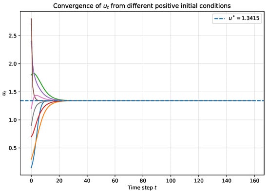
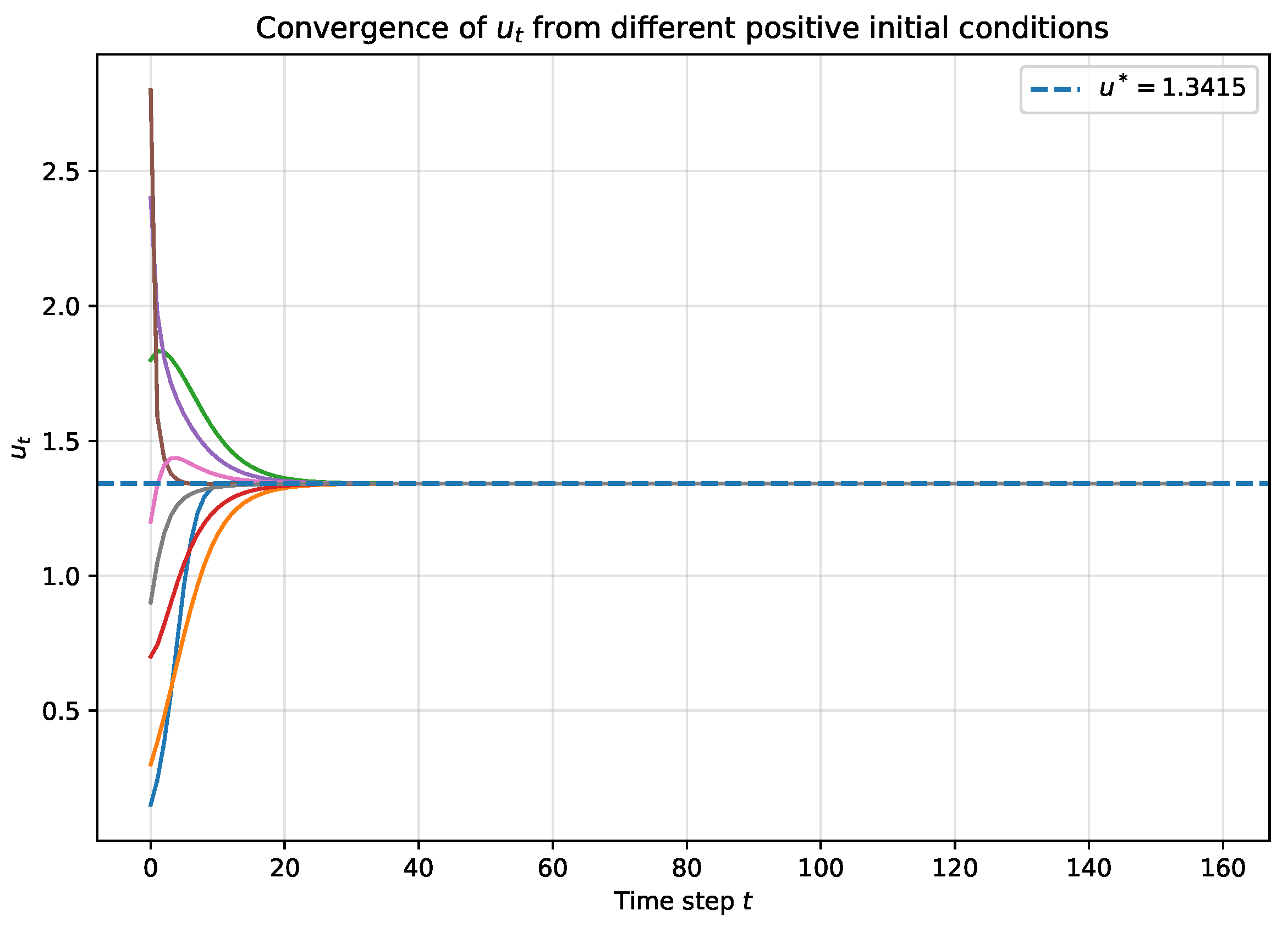
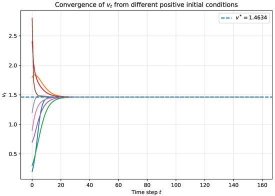
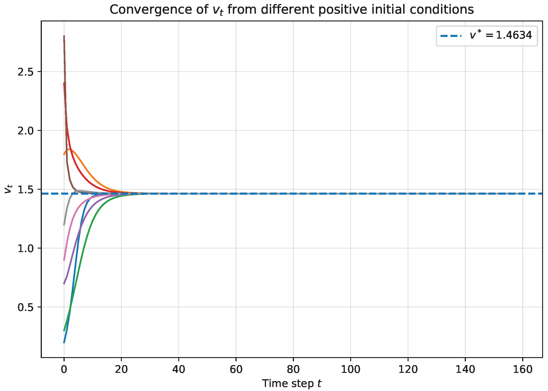
Several distinct positive initial conditions were selected, and the corresponding trajectories of model (2) were computed. Figure 1 and Figure 2 show the time evolution of the variables $u_t$ and $v_t$, respectively. It can be observed that all trajectories converge to the same positive equilibrium point regardless of the initial conditions. These numerical results are consistent with the theoretical prediction of Theorem 8 and provide additional evidence for the global asymptotic stability of the positive equilibrium.

Figure 1. Convergence of $u_t$ toward the positive equilibrium $u^{*}$ from different positive initial conditions. The colored curves correspond to different initial values, while the dashed horizontal line indicates the equilibrium value $u^{*}$.

Figure 2. Convergence of $v_t$ toward the positive equilibrium $v^{*}$ from different positive initial conditions.

Theorem 9.

Model (2) undergoes a flip bifurcation at the positive equilibrium point $E^{*}(u^{*},v^{*})$ if

$$4-2{\displaystyle \frac{a_1+a_2}{a_3}}+{\displaystyle \frac{a_1{a}_2}{a_3}}=0,$$

where

$$a_1=r_1(1-s_1),a_2=r_2(1-s_2),a_3=1-s_1{s}_2.$$

Proof. 

The characteristic polynomial of the Jacobian matrix evaluated at the positive equilibrium point $E^{*}$ is

$$F\left(\lambda \right)={\lambda }^2-T\lambda +D,$$

where

$$T=2-{\displaystyle \frac{a_1+a_2}{a_3}}\mathrm{and}D=1-{\displaystyle \frac{a_1+a_2}{a_3}}+{\displaystyle \frac{a_1{a}_2}{a_3}}.$$

A flip bifurcation occurs when one of the characteristic roots of the Jacobian matrix crosses the unit circle through $\lambda =-1$. Thus, setting $\lambda =-1$ in the characteristic equation gives

$$F(-1)=1+T+D=0.$$

Substituting the expressions of T and D, we obtain

$$1+\left(2-{\displaystyle \frac{a_1+a_2}{a_3}}\right)+\left(1-{\displaystyle \frac{a_1+a_2}{a_3}}+{\displaystyle \frac{a_1{a}_2}{a_3}}\right)=0.$$

After simplification, we derive

$$4-2{\displaystyle \frac{a_1+a_2}{a_3}}+{\displaystyle \frac{a_1{a}_2}{a_3}}=0.$$

Hence, model (2) undergoes a flip bifurcation at the positive equilibrium point $E^{*}(u^{*},v^{*})$. □

Treating $r_1$ as the bifurcation parameter and using

$$a_1=r_1(1-s_1),$$

the flip bifurcation condition obtained in Theorem 9,

$$4-2{\displaystyle \frac{a_1+a_2}{a_3}}+{\displaystyle \frac{a_1{a}_2}{a_3}}=0,$$

can be solved explicitly for $r_1$. This yields

$$r_{1,\mathrm{flip}}={\displaystyle \frac{2a_2-4a_3}{(1-s_1)(a_2-2)}},$$

where

$$a_2=r_2(1-s_2),a_3=1-s_1{s}_2.$$

For the numerical simulations, the parameters were chosen as

$$r_2=1.2,n_1=n_2=2,s_1=0.45,s_2=0.40,$$

we obtain

$$r_{1,\mathrm{flip}}\approx 2.62.$$

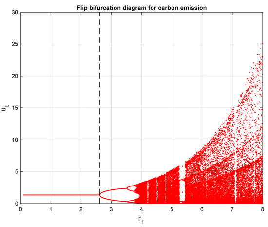
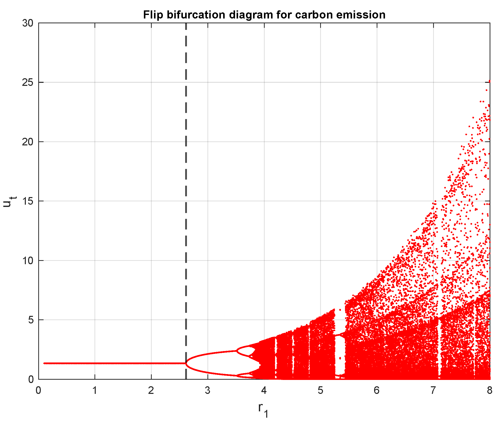
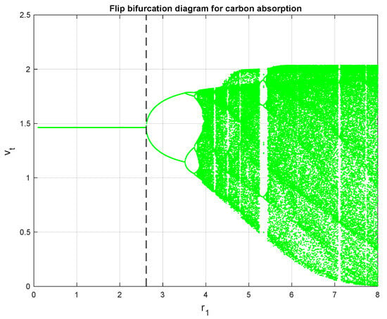
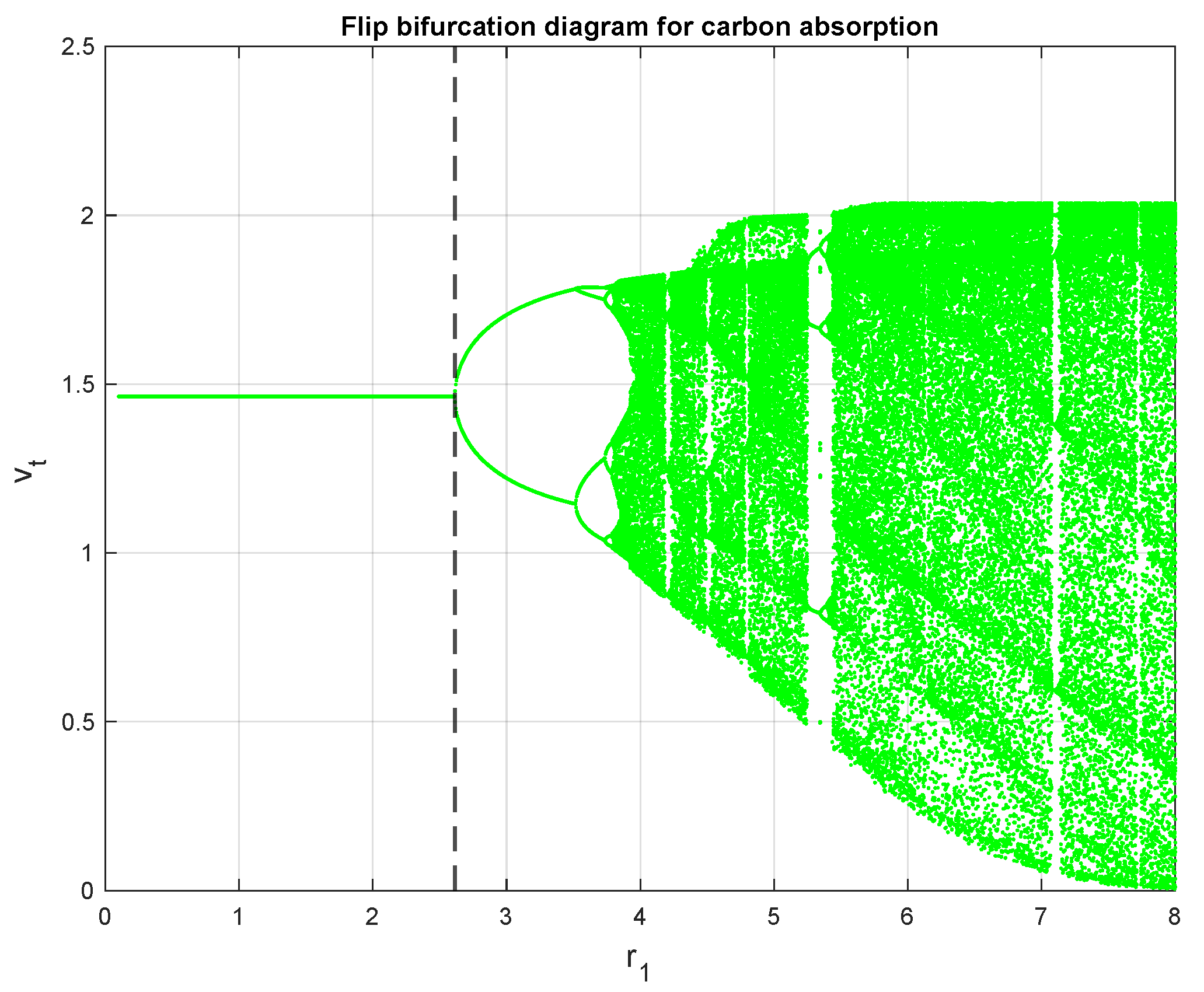
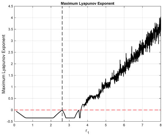
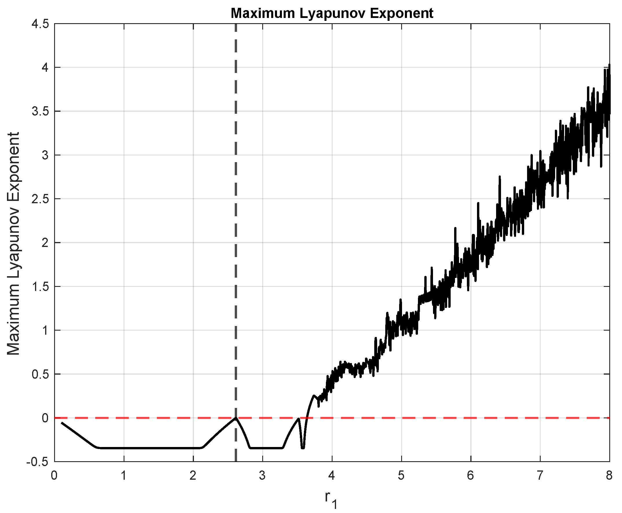
Therefore, the positive equilibrium loses stability through a flip bifurcation when $r_1$ crosses the critical value $r_{1,\mathrm{flip}}$, which is consistent with the numerical bifurcation diagrams presented in Figure 3 and Figure 4. The obtained numerical results show that the positive equilibrium point is locally asymptotically stable for small values of $r_1$. However, when $r_1$ approaches the theoretical critical value $r_{1,\mathrm{flip}}$ the system loses stability through a flip (period-doubling) bifurcation. After this threshold, successive period-doubling oscillations and chaotic dynamics appear in both the carbon emission and carbon absorption variables. Furthermore, as shown in Figure 5, the maximum Lyapunov exponent becomes positive in the chaotic region, confirming the emergence of chaos after the flip bifurcation.

Figure 3. Flip bifurcation diagram for the carbon emission variable $u_t$.

Figure 4. Flip bifurcation diagram for the carbon absorption variable $v_t$.

Figure 5. Maximum Lyapunov Exponent (MLE) corresponding to the flip bifurcation analysis.

3. Turing Instability in the Discrete Diffusion Carbon Model

In this section, we investigate the diffusion-driven instability, also known as Turing instability [15], of the space-time discrete carbon emission-absorption model (3). The main idea is to determine whether the homogeneous positive equilibrium, which is stable in the non-diffusive model (2), becomes unstable when spatial diffusion is introduced. Let $E^{*}(u^{*},v^{*})$ be the positive equilibrium point of model (2), where

$$u^{*}={\displaystyle \frac{n_1(1-s_1)}{1-s_1{s}_2}},v^{*}={\displaystyle \frac{n_2(1-s_2)}{1-s_1{s}_2}}.$$

For simplicity, define

$$a_1=r_1(1-s_1),a_2=r_2(1-s_2),a_3=1-s_1{s}_2.$$

Step 1. Linearization around the homogeneous equilibrium

We introduce small perturbations around $E^{*}$:

$$u_t^{i,j}=u^{*}+{\tilde{u}}_t^{i,j},v_t^{i,j}=v^{*}+{\tilde{v}}_t^{i,j}.$$

Since $E^{*}$ is spatially homogeneous,

$${\nabla }^2{u}^{*}=0,{\nabla }^2{v}^{*}=0.$$

The reaction terms of model (3) are

$$f(u,v)=uexp\left[r_1\left(1-{\displaystyle \frac{u}{n_1}}-{\displaystyle \frac{s_{1}v}{n_2}}\right)\right],$$

and

$$g(u,v)=vexp\left[r_2\left(1-{\displaystyle \frac{v}{n_2}}-{\displaystyle \frac{s_{2}u}{n_1}}\right)\right].$$

The partial derivatives evaluated at $E^{*}$ are

$$f_u\left(E^{*}\right)=1-{\displaystyle \frac{a_1}{a_3}},f_v\left(E^{*}\right)=-{\displaystyle \frac{s_1{a}_1{n}_1}{n_2{a}_3}},$$

and

$$g_u\left(E^{*}\right)=-{\displaystyle \frac{s_2{a}_2{n}_2}{n_1{a}_3}},g_v\left(E^{*}\right)=1-{\displaystyle \frac{a_2}{a_3}}.$$

Therefore, the linearized form of model (3) around $E^{*}$ is

$$\left\{\begin{array}{c}{\tilde{u}}_{t+1}^{i,j}=\left(1-{\displaystyle \frac{a_1}{a_3}}\right){\tilde{u}}_t^{i,j}-{\displaystyle \frac{s_1{a}_1{n}_1}{n_2{a}_3}}{\tilde{v}}_t^{i,j}+d_1{\nabla }^2{\tilde{u}}_t^{i,j},\hfill \\ {\tilde{v}}_{t+1}^{i,j}=-{\displaystyle \frac{s_2{a}_2{n}_2}{n_1{a}_3}}{\tilde{u}}_t^{i,j}+\left(1-{\displaystyle \frac{a_2}{a_3}}\right){\tilde{v}}_t^{i,j}+d_2{\nabla }^2{\tilde{v}}_t^{i,j}.\hfill \end{array}\right.$$

Step 2. Eigenvalue problem of the discrete Laplacian

To study the effect of diffusion, we consider the eigenvalue problem

$${\nabla }^2{X}^{i,j}+\lambda X^{i,j}=0$$

under periodic boundary conditions. Using the approach in [16], the eigenvalues of the discrete Laplacian operator are

$${\lambda }_{sl}=4\left[{sin}^2\left({\displaystyle \frac{(s-1)\pi }{n}}\right)+{sin}^2\left({\displaystyle \frac{(l-1)\pi }{n}}\right)\right]=q_{sl}^2,$$

where

$$s,l\in \{1,2,\dots ,n\}.$$

Thus,

$${\nabla }^2{X}_{sl}^{i,j}=-q_{sl}^2{X}_{sl}^{i,j}.$$

Step 3. Projection onto spatial eigenmodes

Taking the inner product of the linearized system with the eigenfunction $X_{sl}^{i,j}$ corresponding to the eigenvalue $q_{sl}^2$, we obtain

$${\displaystyle \sum _{i,j=1}^n}{X}_{sl}^{i,j}{\tilde{u}}_{t+1}^{i,j}=\left(1-{\displaystyle \frac{a_1}{a_3}}\right){\displaystyle \sum _{i,j=1}^n}{X}_{sl}^{i,j}{\tilde{u}}_t^{i,j}-{\displaystyle \frac{s_1{a}_1{n}_1}{n_2{a}_3}}{\displaystyle \sum _{i,j=1}^n}{X}_{sl}^{i,j}{\tilde{v}}_t^{i,j}+d_1{\displaystyle \sum _{i,j=1}^n}{X}_{sl}^{i,j}{\nabla }^2{\tilde{u}}_t^{i,j},$$

and

$${\displaystyle \sum _{i,j=1}^n}{X}_{sl}^{i,j}{\tilde{v}}_{t+1}^{i,j}=-{\displaystyle \frac{s_2{a}_2{n}_2}{n_1{a}_3}}{\displaystyle \sum _{i,j=1}^n}{X}_{sl}^{i,j}{\tilde{u}}_t^{i,j}+\left(1-{\displaystyle \frac{a_2}{a_3}}\right){\displaystyle \sum _{i,j=1}^n}{X}_{sl}^{i,j}{\tilde{v}}_t^{i,j}+d_2{\displaystyle \sum _{i,j=1}^n}{X}_{sl}^{i,j}{\nabla }^2{\tilde{v}}_t^{i,j}.$$

Let

$$U_t={\displaystyle \sum _{i,j=1}^n}{X}_{sl}^{i,j}{\tilde{u}}_t^{i,j},V_t={\displaystyle \sum _{i,j=1}^n}{X}_{sl}^{i,j}{\tilde{v}}_t^{i,j}.$$

Using the periodic boundary conditions and

$${\nabla }^2{X}_{sl}^{i,j}=-q_{sl}^2{X}_{sl}^{i,j},$$

we obtain

$$\left(\begin{array}{c}{U}_{t+1}\\ V_{t+1}\end{array}\right)=J_{q_{sl}}\left(\begin{array}{c}{U}_t\\ V_t\end{array}\right),$$

where

$$J_{q_{sl}}=\left(\begin{array}{cc}1-{\displaystyle \frac{a_1}{a_3}}-d_1{q}_{sl}^2& -{\displaystyle \frac{s_1{a}_1{n}_1}{n_2{a}_3}}\\ -{\displaystyle \frac{s_2{a}_2{n}_2}{n_1{a}_3}}& 1-{\displaystyle \frac{a_2}{a_3}}-d_2{q}_{sl}^2\end{array}\right).$$

Proposition 1.

If $(U_t,V_t)$ is a solution of the reduced mode system

$$\left(\begin{array}{c}{U}_{t+1}\\ V_{t+1}\end{array}\right)=J_{q_{sl}}\left(\begin{array}{c}{U}_t\\ V_t\end{array}\right),$$

then

$${\tilde{u}}_t^{i,j}=U_t{X}_{sl}^{i,j},{\tilde{v}}_t^{i,j}=V_t{X}_{sl}^{i,j}$$

is also a solution of the linearized perturbation system of model (3) under periodic boundary conditions. Therefore, instability of the reduced mode system implies instability of the corresponding spatial mode of the discrete diffusion carbon model.

Step 4. Characteristic polynomial of the spatial mode

The characteristic polynomial associated with $J_{q_{sl}}$ is

$$F_{q_{sl}}\left(\lambda \right)={\lambda }^2-T_{q_{sl}}\lambda +\mathrm{Det}{J}_{q_{sl}},$$

where

$$T_{q_{sl}}=2-{\displaystyle \frac{a_1+a_2}{a_3}}-(d_1+d_2)q_{sl}^2,$$

and

$$\begin{array}{cc}\hfill \mathrm{Det}{J}_{q_{sl}}& =d_1{d}_2{q}_{sl}^4\hfill \\ & -\left[d_1\left(1-{\displaystyle \frac{a_2}{a_3}}\right)+d_2\left(1-{\displaystyle \frac{a_1}{a_3}}\right)\right]q_{sl}^2\hfill \\ & +\left[1-{\displaystyle \frac{a_1+a_2}{a_3}}+{\displaystyle \frac{a_1{a}_2}{a_3}}\right].\hfill \end{array}$$

Combining these results with Property 1 in [17], the following theorem can be established.

Step 5. Turing instability criterion

Theorem 10.

(3) is unstable at the equilibrium point $E^{*}(u^{*},v^{*})$ if there exists an eigenvalue $q_{sl}^2$ and positive diffusion coefficients $d_1,d_2$ such that one of the following conditions holds:

$$\mathrm{Det}{J}_{q_{sl}}<(d_1+d_2)q_{sl}^2-3+{\displaystyle \frac{a_1+a_2}{a_3}},$$

or

$$\mathrm{Det}{J}_{q_{sl}}<-(d_1+d_2)q_{sl}^2+1-{\displaystyle \frac{a_1+a_2}{a_3}},$$

or

$$\mathrm{Det}{J}_{q_{sl}}>1.$$

Proof. 

For the reduced mode system, the characteristic polynomial is

$$F_{q_{sl}}\left(\lambda \right)={\lambda }^2-T_{q_{sl}}\lambda +\mathrm{Det}{J}_{q_{sl}}.$$

Equivalently,

$$F_{q_{sl}}\left(\lambda \right)={\lambda }^2+b_{q_{sl}}\lambda +\mathrm{Det}{J}_{q_{sl}},$$

where

$$b_{q_{sl}}=-T_{q_{sl}}=(d_1+d_2)q_{sl}^2-2+{\displaystyle \frac{a_1+a_2}{a_3}}.$$

According to the stability criterion for second-order discrete characteristic polynomials, the roots lie inside the unit circle if and only if

$$b_{q_{sl}}-1<\mathrm{Det}{J}_{q_{sl}},$$

$$-b_{q_{sl}}-1<\mathrm{Det}{J}_{q_{sl}},$$

and

$$\mathrm{Det}{J}_{q_{sl}}<1.$$

Therefore, the reduced mode system becomes unstable if one of these inequalities is violated, namely

$$\mathrm{Det}{J}_{q_{sl}}<b_{q_{sl}}-1,\mathrm{or}\mathrm{Det}{J}_{q_{sl}}<-b_{q_{sl}}-1,\mathrm{or}\mathrm{Det}{J}_{q_{sl}}>1.$$

Substituting

$$b_{q_{sl}}=(d_1+d_2)q_{sl}^2-2+{\displaystyle \frac{a_1+a_2}{a_3}},$$

we obtain

$$\mathrm{Det}{J}_{q_{sl}}<(d_1+d_2)q_{sl}^2-3+{\displaystyle \frac{a_1+a_2}{a_3}},$$

or

$$\mathrm{Det}{J}_{q_{sl}}<-(d_1+d_2)q_{sl}^2+1-{\displaystyle \frac{a_1+a_2}{a_3}},$$

or

$$\mathrm{Det}{J}_{q_{sl}}>1.$$

Hence, if at least one of these conditions holds for some nonzero spatial mode $q_{sl}^2>0$, then the corresponding mode becomes unstable while the homogeneous equilibrium remains stable in the non-diffusive system. Therefore, the instability is induced by diffusion, and model (3) undergoes diffusion-driven instability, also called Turing instability. □

4. Machine Learning Approach

Since the local stability of the discrete carbon emission-absorption model is rigorously established by analytical methods, exploring the influence of the parameter space

$$(r_1,r_2,s_1,s_2,n_1,n_2)$$

on system behavior can be computationally demanding. Therefore, machine learning (ML) classification techniques are introduced as a complementary exploratory tool to approximate the stability structure of the model.

A synthetic training dataset is generated through Monte Carlo sampling of the parameter space of model (2). For each sampled parameter set, the stability type of the interior equilibrium point $E^{*}$ is determined using the analytically derived Jacobian eigenvalue conditions as the ground truth. Based on this labeled dataset, Decision Tree and Random Forest classifiers are trained to predict the stability regimes, namely sink, source, saddle, and nonhyperbolic cases. The dataset is divided into training and testing subsets using a stratified 75%/25% split, preserving the class distribution in both subsets.

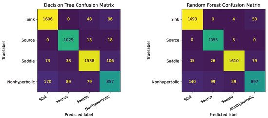
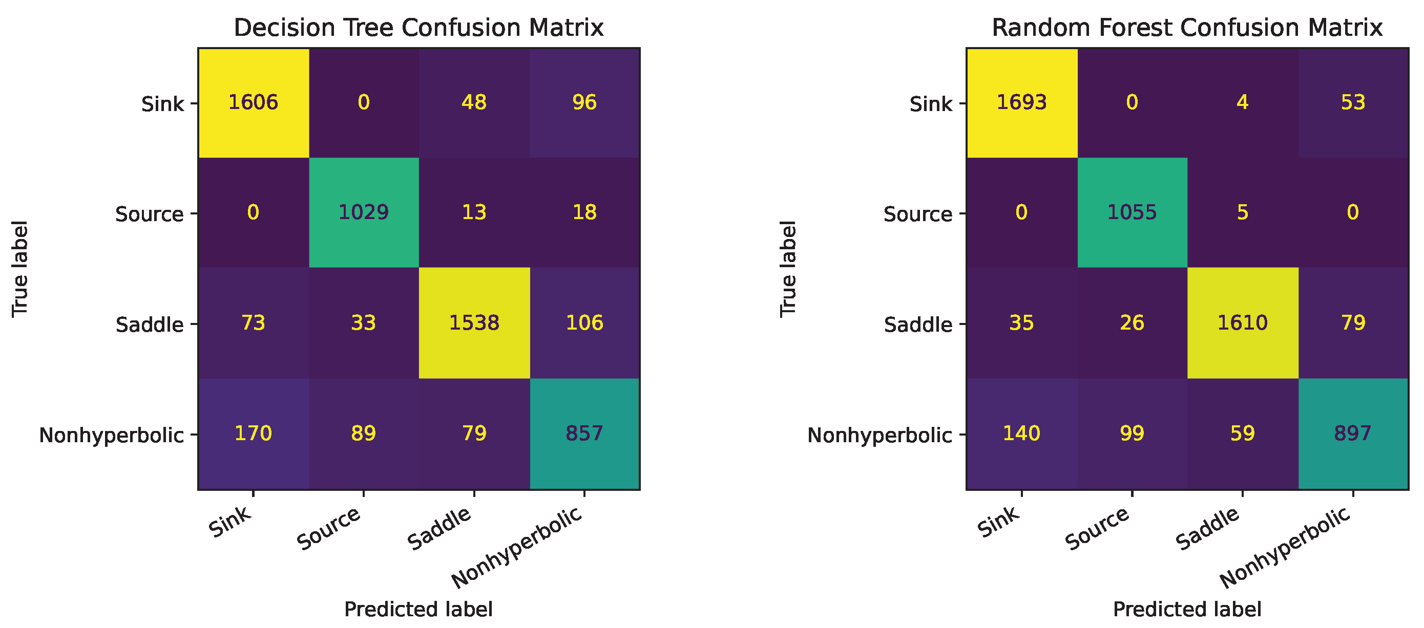
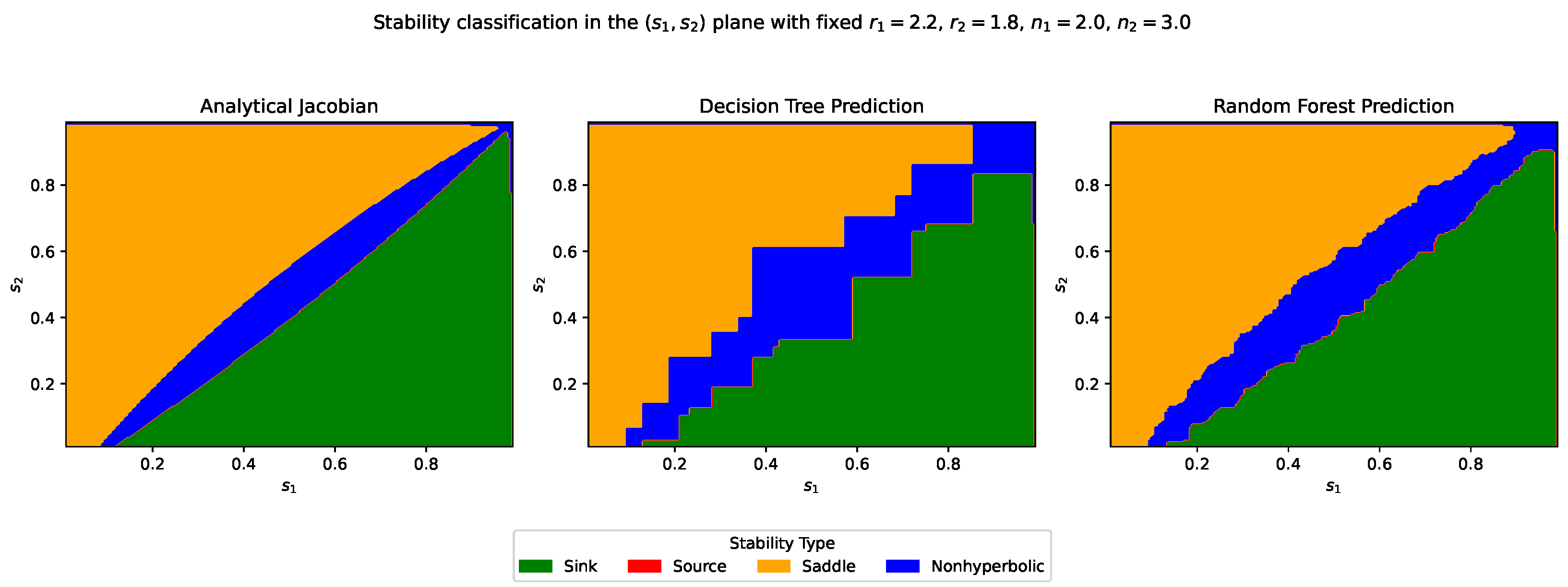
The numerical results show that the Decision Tree classifier achieves a test accuracy of $87.40\%$, whereas the Random Forest classifier achieves a higher test accuracy of $91.31\%$. This indicates that the Random Forest model more effectively approximates the analytically derived stability regions and provides smoother classification boundaries.

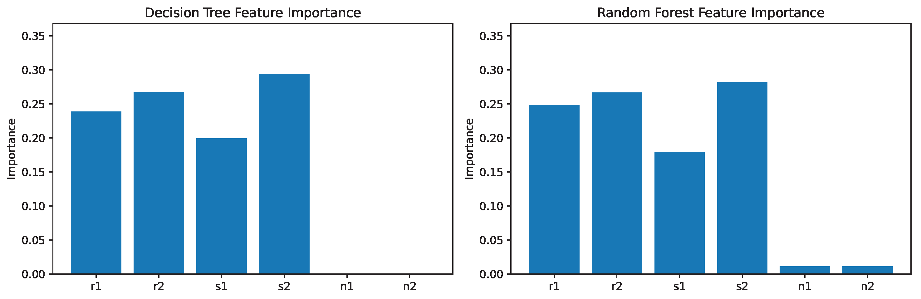
It is important to emphasize that the present ML analysis serves as a computational validation tool rather than a source of new theoretical results. By reproducing analytically derived stability regions, the ML classifiers confirm their effectiveness as surrogate approximators of complex parameter-stability relationships. It should be noted that the analytical stability conditions remain the exact criterion for stability classification in the present model. The machine learning classifiers are introduced to investigate whether data-driven methods can recover the analytically derived stability structure and thereby serve as computational surrogates for more complex dynamical systems where explicit analytical conditions may not be available. This framework provides a promising direction for future research, particularly for high-dimensional extensions of the model or data-driven studies where analytical methods become intractable. The corresponding classification reports and visual comparisons of the analytically derived and machine-learning-based stability regions are presented in Table 3 and Table 4 and Figure 6, Figure 7 and Figure 8.

Table 3. Decision Tree classification report based on the Monte Carlo dataset.

Class	Precision	Recall	F1-Score	Support
Sink	0.8686	0.9177	0.8925	1750
Source	0.8940	0.9708	0.9308	1060
Saddle	0.9166	0.8789	0.8973	1750
Nonhyperbolic	0.7957	0.7172	0.7544	1195
Accuracy	–	–	0.8740	5755
Macro avg	0.8687	0.8711	0.8687	5755
Weighted avg	0.8727	0.8740	0.8723	5755

Table 4. Random Forest classification report based on the Monte Carlo dataset.

Class	Precision	Recall	F1-Score	Support
Sink	0.9063	0.9674	0.9359	1750
Source	0.8941	0.9953	0.9420	1060
Saddle	0.9595	0.9200	0.9393	1750
Nonhyperbolic	0.8717	0.7506	0.8067	1195
Accuracy	–	–	0.9131	5755
Macro avg	0.9079	0.9083	0.9060	5755
Weighted avg	0.9130	0.9131	0.9112	5755

Figure 6. Confusion matrices of the Decision Tree and Random Forest classifiers obtained from the Monte Carlo dataset. The Random Forest classifier provides a more accurate classification performance.

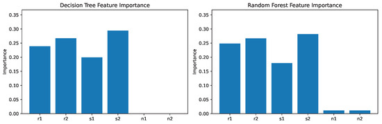
Figure 7. Feature importance values obtained from the Decision Tree and Random Forest classifiers using the Monte Carlo dataset. The parameters $r_1$, $r_2$, and $s_2$ are identified as the dominant factors governing the stability classification, while $n_1$ and $n_2$ have comparatively minor influence.

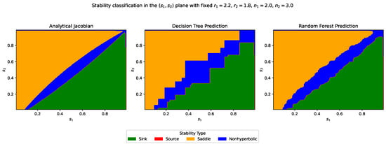
Figure 8. Stability classification in the $(s_1,s_2)$-plane with fixed $r_1=2.2$, $r_2=1.8$, $n_1=2.0$, and $n_2=3.0$. The left panel shows the analytically derived stability regions based on the Jacobian matrix, while the middle and right panels present the Decision Tree and Random Forest predictions, respectively. The Random Forest classifier reproduces the analytical stability boundaries more accurately and smoothly.

5. Conclusions

In this study, a discrete carbon emission-absorption model derived from its continuous counterpart via the piecewise constant argument (PCA) approach was investigated. The proposed model describes the nonlinear interaction between carbon emission and carbon absorption processes and provides a discrete-time framework suitable for analyzing their long-term dynamical behavior.

First, the existence conditions of the equilibrium points were established analytically. Then, the local stability properties of the trivial, boundary, and positive equilibrium points were investigated through Jacobian analysis and characteristic polynomial techniques. In addition, the uniform boundedness of all positive solutions was verified. By employing an iterative method, the global asymptotic stability of the positive equilibrium point was rigorously proved under appropriate parameter conditions.

Furthermore, the dynamical structure of the model was analyzed through bifurcation theory. In particular, the conditions for flip bifurcation were derived analytically, and numerical simulations confirmed the emergence of period-doubling oscillations and chaotic dynamics after the critical bifurcation threshold. The corresponding bifurcation diagrams and maximum Lyapunov exponent plots illustrated the transition from stable dynamics to chaos.

In addition, the diffusion-driven dynamics of the discrete spatial model were investigated through Turing instability analysis. The obtained results showed that spatial diffusion can destabilize the homogeneous equilibrium state and induce diffusion-driven spatial instability in the carbon emission–absorption system. From an environmental perspective, this indicates that spatial interactions and diffusion processes may generate heterogeneous carbon distribution patterns across different regions, which can significantly influence ecosystem balance and long-term environmental sustainability.

Moreover, machine learning approaches based on Decision Tree (DT) and Random Forest (RF) classifiers were employed to approximate the analytically derived stability regions. Training data were generated through Monte Carlo sampling of the parameter space, and the stability types obtained from the analytical Jacobian conditions were used as the ground truth labels. The numerical results demonstrated that the Random Forest classifier achieved higher classification accuracy and reproduced the analytical stability boundaries more effectively than the Decision Tree classifier. Feature importance analysis further indicated that the parameters $r_1$, $r_2$, and $s_2$ play dominant roles in determining the stability behavior of the system.

Overall, the proposed unified framework combines nonlinear dynamical analysis and machine learning techniques to provide a systematic and computationally efficient approach for investigating the stability structure and long-term behavior of carbon emission-absorption systems, thereby contributing to a better understanding of complex carbon processes and environmental sustainability.

References

- Han, X.; Lei, C. Bifurcation and Turing instability analysis for a space-and time-discrete predator-prey system with Smith growth function. Chaos Solitons Fractals 2023, 166, 112910. [Google Scholar] [CrossRef] [Scilit]
- Malchow, H.; Petrovskii, S.V.; Venturino, E. Spatiotemporal Patterns in Ecology and Epidemiology: Theory, Models, and Simulation; Chapman & Hall/CRC: Boca Raton, FL, USA, 2008. [Google Scholar]
- Maynard-Smith, J. Models in Ecology; Cambridge University Press: Cambridge, UK, 1974. [Google Scholar]
- Wiggins, S. Introduction to Applied Nonlinear Dynamical Systems and Chaos; Springer: New York, NY, USA, 2003. [Google Scholar]
- Hou, Y.; Wei, C.; Ding, Y. Dynamic analysis of reaction-diffusion dual carbon model considering economic development in China. Electron. Res. Arch. 2023, 31, 2483–2500. [Google Scholar] [CrossRef] [Scilit]
- Baydemir, P.; Merdan, H. Bifurcation analysis, chaos control, and FAST approach for the complex dynamics of a discrete-time predator–prey system with a weak Allee effect. Chaos Solitons Fractals 2025, 196, 116317. [Google Scholar] [CrossRef] [Scilit]
- Abbasi, M.A. Analyzing global patterns, stability, bifurcation, and chaos control of an ecological model: MA Abbasi. Int. J. Dyn. Control 2025, 13, 151. [Google Scholar] [CrossRef] [Scilit]
- Celik, C.; Duman, O. Allee effect in a discrete-time predator–prey system. Chaos Solitons Fractals 2009, 40, 1956–1962. [Google Scholar] [CrossRef] [Scilit]
- Du, X.; Han, X. Dynamics analysis of a discrete diffusion predator–prey model with prey refuge. J. Comput. Appl. Math. 2025, 470, 116706. [Google Scholar] [CrossRef] [Scilit]
- Mehmood, T.; Rafaqat, M.; Saleem, S.; Merga, F.E. Machine learning and bifurcation analysis in a discrete predator-prey model with neem-induced mortality. Sci. Rep. 2025, 15, 40792. [Google Scholar] [CrossRef] [Scilit]
- Bibi, A.; Mehmood, T.; El-Rehman, M.A.; Rafaqat, M.; Saeed, S.T.; Merga, F.E. Stability and Bifurcation in a Discrete-Time Guava Pest Control Model with Natural Predation and Neem Extract. Math. Methods Appl. Sci. 2026, 1–17. [Google Scholar] [CrossRef] [Scilit]
- Liu, X.; Xiao, D. Complex dynamic behaviors of a discrete-time predator–prey system. Chaos Solitons Fractals 2007, 32, 80–94. [Google Scholar]
- Yang, X. Uniform persistence and periodic solutions for a discrete predator–prey system with delays. J. Math. Anal. Appl. 2006, 316, 161–177. [Google Scholar] [CrossRef] [Scilit]
- Chen, G.; Teng, Z.; Hu, Z. Analysis of stability for a discrete ratio-dependent predator-prey system. Indian J. Pure Appl. Math. 2011, 42, 1–26. [Google Scholar] [CrossRef] [Scilit]
- Turing, A.M. The chemical basis of morphogenesis. Bull. Math. Biol. 1990, 52, 153–197. [Google Scholar] [CrossRef] [Scilit] [PubMed]
- Bai, L.; Zhang, G. Nontrivial solutions for a nonlinear discrete elliptic equation with periodic boundary conditions. Appl. Math. Comput. 2009, 210, 321–333. [Google Scholar] [CrossRef] [Scilit]
- Han, Y.T.; Han, B.; Zhang, L.; Xu, L.; Li, M.F.; Zhang, G. Turing instability and wave patterns for a symmetric discrete competitive Lotka-Volterra system. WSEAS Trans. Math. 2011, 10, 181–189. [Google Scholar]
Disclaimer/Publisher’s Note: The statements, opinions and data contained in all publications are solely those of the individual author(s) and contributor(s) and not of MDPI and/or the editor(s). MDPI and/or the editor(s) disclaim responsibility for any injury to people or property resulting from any ideas, methods, instructions or products referred to in the content. |
© 2026 by the authors. Licensee MDPI, Basel, Switzerland. This article is an open access article distributed under the terms and conditions of the Creative Commons Attribution (CC BY) license.