


Abstract
The study is driven by its importance in modern material processing and precision engineering, where understanding and controlling interfacial stability is crucial in maintaining reliable performance across various operating conditions. The interplay between the tangential magnetic field and temporal periodicity generates additional mechanisms of mode coupling and amplifies instability. These observations address critical shortcomings in nonlinear stability theory and suggest practical uses in flow regulation and the control of conductive fluids. The fluids are assumed as Eyring–Powell non-Newtonian and flow with uniform velocities through porous media. The analysis is conducted using a non-perturbative method that relies mainly on He’s frequency formulation. To facilitate the mathematical treatment, viscous potential theory is adopted. The governing linear partial differential equations describing the flow are then solved under nonlinear boundary conditions, resulting in a nonlinear characteristic equation that represents the displacement of the interface. A non-dimensional procedure is then applied to extract the key dimensionless physical parameters influencing the system behavior. A set of graphical results is provided to demonstrate how the system’s stability behavior is influenced by changes in the key dimensionless physical parameters. The validation of the innovative process is achieved using Mathematica Software. The study considers both uniform and periodically varying magnetic fields, and the associated stability conditions are evaluated for each case, where the impacts of various non-dimensional attributes are assessed. As density ratio increases, it stabilizes periodic magnetic fields while destabilizing uniform ones. A stronger MF enhances magnetic damping, reducing instability regions and promoting stable periodic interfacial motion. Enhanced conductivity improves Magnetohydrodynamic interactions, resulting in greater energy dissipation and stability.
Keywords:
nonlinear systems; mathematical model; Eyring–Powell fluid; periodic magnetic field; viscous potential theory; non-perturbative method; differential equations; numerical results MSC:
35Q35; 76E17; 34C15; 76W05
1. Introduction
Ferromagnetic fluids are typically produced under controlled laboratory conditions [1]. These materials are composed of a colloidal mixture in which fine ferrite particles are dispersed within a carrier liquid. To avoid particle accumulation similar to the behavior of iron filings in magnetic environments, the particle sizes are significantly reduced and thermal motion promotes a strong diffusive effect. Consequently, the fluid behaves like an ordinary liquid while remaining responsive to forces generated by magnetic polarization. This study investigates the modification of stability at a planar interface separating two ferromagnetic fluids subjected to a uniform normal MF and gravitational effects. In general, MFs consist of very small magnetic particles suspended in electrically insulating liquids, behaving as a single continuous medium and exhibiting various unique physical phenomena [2]. Due to their wide range of industrial applications, magnetic fluids have attracted increasing attention, particularly under both normal and tangential MF configurations. Many engineering systems involve the simultaneous flow of fluids with different viscosities and densities through porous media [3]. The study of peristaltic transport in non-Newtonian fluids has gained significant attention due to its applications in biomedical and engineering systems. Studies such as that of Akbar and Nadeem [4] have examined the peristaltic flow of nanofluids under specific physical conditions, emphasizing the influence of wall motion and transport mechanisms on flow characteristics. Investigations were carried out on the Sutterby fluid model within symmetric vertical channels under conditions of high mass transfer. Similar flow mechanisms arise in packed-bed reactors, chemical processing systems, petroleum engineering, and heat transfer processes in porous structures. Furthermore, earlier work by Melcher demonstrated that a flat interface between two immiscible fluids when at least one of them was ferromagnetic may become unstable under the influence of an externally applied normal MF [5]. The Kelvin–Helmholtz instability (KHI) has been extensively used to analyze the interfacial instability between fluid layers, including ferrofluid systems and porous configurations [6]. Classical and modern stability theories have provided fundamental insights into the onset and evolution of such instabilities under various physical effects [7]. In this configuration, the fluids were separated by an infinitely long vertical cylindrical interface. In addition, the KHI of stratified ferrofluids subjected to rotational effects and a time-periodic tangential MF was studied [8], where each fluid layer possesses distinct constant densities and moves with different uniform velocities. Electro-osmotic transport of non-Newtonian fluids has also attracted increasing attention, particularly in microfluidic applications, where electric fields significantly influence flow characteristics. Several studies have provided analytical and numerical solutions describing electro-osmotic effects in viscoelastic and non-Newtonian fluids [9]. Furthermore, the combined effects of thermal radiation and MFs on nanofluid behavior have attracted considerable attention due to their relevance in biomedical and therapeutic applications [10]. In this context, the effectiveness of gold nanoparticles dispersed in blood flow modeled as a Sisko fluid over a lubricated porous curved surface was analyzed, with results showing strong agreement when compared with previously reported findings. The NPA diverges from previous models by including and addressing particular deficiencies highlighted in past studies. This gap is not merely gradual but represents substantial methodological advancement. We believe this explanation highlights the uniqueness and significance of the proposed methodology, and we are prepared to revise the work to elucidate this distinction if necessary.
The EPF represents a class of non-Newtonian viscoelastic fluids originally introduced in 1944. Although it was addressed in several studies, it remains relatively underexplored in the literature. Previous investigations have analyzed electrophoretic fluid flow incorporating the effects of MHD and Joule heating [11], where the bounding surface was assumed to oscillate with a power-law velocity profile about a slit. Such configurations can be extended to more complex geometries, including cylindrical and wedge-shaped domains, to broaden the scope of analysis. A comprehensive understanding of fluid behavior also requires consideration of different thermal boundary conditions, such as imposed heat flux and Newtonian heating. In this context, EPF flow applied as a coating over a wire was studied by accounting for variations in viscosity, thermal radiation, and Joule dissipation effects [12]. Furthermore, the role of hybrid nanoparticles in enhancing thermal performance during peristaltic transport of EPF was examined [13]. Despite these contributions, research on this specific subclass of fluids remains limited, and a complete survey of the available literature is beyond the present scope. The EPF plays an important role in fluid mechanics, with applications in viscosity evaluation, chemical reaction modeling, atomic diffusion processes, polymer engineering, and lubrication systems. For instance, two-dimensional sinusoidal transport of EPF in a porous medium bounded by peristaltic surfaces was analyzed using water as the base fluid [14], where the governing PDEs of motion and heat transfer were solved using semi-analytical techniques based on classical perturbation methods and the Navier–Stokes framework. Additionally, MHD heat transfer in fluids with variable thermophysical properties, particularly EPF, was widely investigated due to its complex rheological behavior [15]. The influence of MHD flow over a shrinking or contracting surface was explored [16]. Other studies have considered the combined effects of temperature-dependent viscosity and thermal conductivity on flow and heat transport in EPF systems, including the contribution of nonlinear thermal radiation [17]. Moreover, the complex swirling motion of non-Newtonian electro-rheological fluids confined between two coaxial rotating disks was examined, where each disk rotates with a different angular velocity [18].
A large body of research has focused on various types of oscillatory systems due to their wide-ranging applications in physics and engineering. Approximate analytical solutions were obtained using different techniques, including the HPM combined with the Aboodh transform [19]. In addition, Wang proposed an alternative framework based on the Rayleigh–Ritz technique, enhanced through an extended Galerkin formulation, providing improved analytical capabilities [20]. Consequently, many oscillators of physiological relevance were examined as particular cases within these approaches. In further studies, nonlinear oscillators incorporating two characteristic length scales were analyzed [21,22], where the geometric configuration involves a parabola rotating about its vertical axis with a constant angular velocity. This configuration leads to a highly nonlinear ODE governing the system dynamics. Approximate solutions were derived by integrating HPM with the Laplace transform, while nonlinear frequency methods were employed to obtain periodic solutions. These approaches allow for the establishment of stability criteria through frequency-based analysis. Given the broad importance of oscillatory systems in disciplines such as engineering, electronics, physics, chemistry, and biology, numerous analytical and numerical techniques were developed to study equations like the van der Pol oscillator. Classical solution methods often attempt to account for secular terms; however, such approaches typically fail to eliminate these terms completely. Moreover, extensions based on modified frequency concepts generally yield only limited accuracy. To address these limitations, an improved version of the residual error minimization technique was introduced for solving the nonlinear third-order Jerk ODE [23]. Two representative cases were presented to validate the efficiency of this method. The obtained results were compared with exact NSs derived from the Navier–Stokes equations as well as previously reported methods. This comparison demonstrated that the proposed approach offers higher accuracy and represents a significant improvement over earlier solution techniques.
The shortcomings associated with conventional perturbation techniques were addressed through the development of more advanced analytical methods, including improved perturbation schemes and complementary tools such as vibration theory, the HPM, and iterative procedures. Studies on both weakly and strongly nonlinear systems were extensively reported using asymptotic approaches [24], with particular emphasis on developments achieved in China within this research area. Several analytical frameworks were proposed in examining nonlinear oscillators, among which HFF, the max–min method, and HPM represent major methodological contributions [25]. Refinements in mathematical regularization have further enhanced the accuracy of frequency estimation techniques. In addition, highly nonlinear oscillatory systems were investigated through direct and more generalized control strategies [26], demonstrating that these methods can yield highly accurate results. Moreover, efficient analytical techniques were introduced to rapidly evaluate the relationship between amplitude and frequency in nonlinear oscillators using simplified solution procedures. This amplitude–frequency correlation was applied in various engineering contexts, including packaging structures and emerging micro-electro-mechanical systems [27]. Such developments contributed to a deeper understanding of nonlinear vibrational behavior and have enabled straightforward computational approaches for determining oscillation frequencies under different ICs. Recent publications in fluid mechanics and dynamic systems were produced, as indicated by NPA [28,29,30]. Research was conducted on non-submerged jet icebreaking for surface vessels [31]. Submerged jet icebreaking for underwater vehicles was not conducted. A nonlinear creep model incorporating damage factors based on irreversible deformation was suggested, quantitatively representing the perturbation aftereffect characterized by rapid creep progression resulting from minor disturbances [32]. The model effectively represented the nonlinearity of rock mass creep deformation and the residual impacts of previous disturbances, thus addressing the constraints of existing models in integrating the interactions between long-term creep and short-term perturbations. The hydrodynamic force on the submerged cylinder was assessed, utilizing the acceleration potential method in conjunction with a singularized boundary integral approach [33]. A slot hole and a design strategy of the exit edge angle were analyzed [34]. NSs and pressure-sensitive paint measurements were employed to elucidate the jet-flow-field features at various exit edge angles, and the comprehensive surface distribution of film cooling effectiveness at a density ratio of 3.0 was acquired. The following details of NPA or notable accomplishments must be emphasized:
- The unique technique produces a new linear ODE that is compatible with the original nonlinear one.
- The MS reveals that the two ODEs demonstrate a definitive association in this novel technique.
- The traditional perturbation approaches complicate the current inquiry by amplifying the restorative operations at their respective sites via Taylor expansion. The NPA alleviates this vulnerability.
- The NPA enables us to investigate the stability issue in contrast to traditional perturbation techniques.
- The innovative method appears to be a straightforward, rational, and engaging tool.
The experimental investigation of nonlinear instability in a fluid jet subjected to a tangential periodic MF establishes a crucial link between fundamental fluid dynamics and practical technology applications. By carefully designing laboratory setups, often employing electrically conductive fluids such as liquid metals or electrolytes, researchers can directly investigate the effects of magnetic forces on wave amplification, jet disintegration, and pattern formation beyond the linear regime. These tests illustrate intricate phenomena including mode coupling, harmonic amplification, and controlled destabilization, which are essential in validating theoretical and computational models of nonlinear systems. These insights have significant implications in fields necessitating precise fluid flow control: in metallurgy, MFs can mitigate or exacerbate instabilities during casting; in microfluidics, they enable non-contact manipulation of jets for lab-on-a-chip applications; and in energy systems, especially cooling technologies employing liquid metals, understanding these instabilities helps prevent unwanted turbulence or destruction. The ability to modify instability characteristics through periodic magnetic forcing presents prospects of advanced flow control methods, allowing engineers to deliberately induce or alleviate nonlinear phenomena to improve mixing, heat transfer, or material uniformity. For the sake of clarity and to avoid unnecessary mathematical complexity, the detailed nonlinear governing PDEs are not explicitly presented here. Therefore, this aspect is not further addressed in the current discussion. The nonlinear interfacial instability of a ferromagnetic fluid jet arises from the intricate interplay between ST, magnetic forces, and hydrodynamic effects. When subjected to MFs, the interface behavior deviates from that governed solely by ST, leading to increasingly complex and sometimes unpredictable jet configurations, including possible breakup phenomena. The primary objective of this study is to analyze the nonlinear interfacial instability of a ferromagnetic fluid jet using an NPA. For clarity, the structure of this paper is organized as follows: Section 2 presents the mathematical formulation of the physical model, including the governing PDEs and the required BCs. In Section 3, the nonlinear characteristic ODE describing interface displacement is derived. The solution methodology is detailed in Section 4. The case of a periodic MF is discussed in Section 5, while the uniform MF scenario is considered in Section 6. The obtained results and their discussion are provided in Section 7, and the main conclusions are summarized in Section 8.
2. Description and Formulation
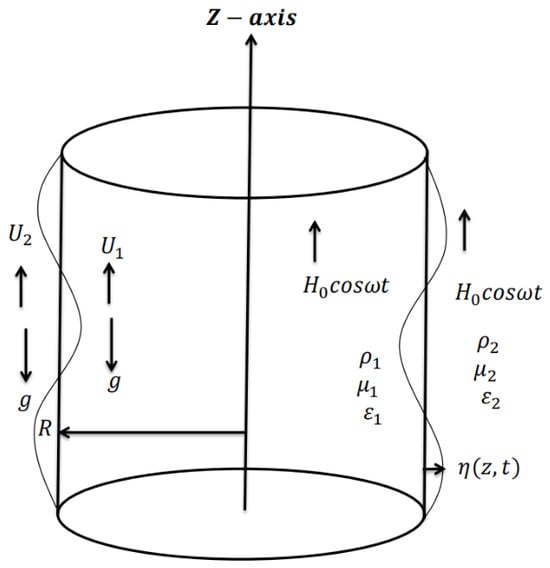
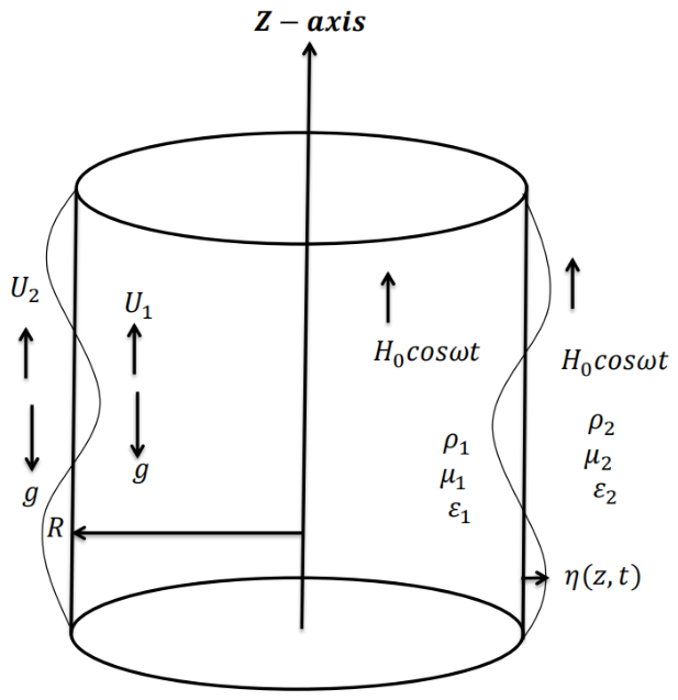
The complicated interaction between hydrodynamic forces and an externally applied MF controls interfacial instability of a ferromagnetic jet under nonlinear effects. This interaction is investigated when a periodic MF is introduced, adding more temporal modulation to the system. Nonlinear dynamics, such as parametric amplification of disturbances, can be produced by such modulation and may eventually result in jet breakup or the creation of complex interfacial structures. This study investigates an indefinitely long cylindrical jet made up of two non-Newtonian EPFs that are immiscible and incompressible. A periodic MF applied along the jet’s axis can be described as follows: , with k being the axial wave number and ω indicating the frequency of oscillation. Gravitational effects are also considered, while assuming an absence of free electric currents within the fluid domain [35]. The governing PDEs are expressed in cylindrical coordinates for mathematical convenience, with the axis parallel to the jet’s equilibrium state. Different densities and magnetic permeabilities distinguish the inner and surrounding fluids. It is assumed that both fluids travel in the positive direction with constant axial velocities, . The symbol stands for the jet’s unperturbed radius, while the inner and outer areas are labeled with subscripts , respectively. Using Darcy’s law for an incompressible fluid in a homogeneous and isotropic medium, the formulation also considered across porous media. Here, the fluid viscosity and permeability parameter are represented by the expression . Both media are considered to have unit porosity for simplicity’s sake. Therefore, Figure 1 shows a schematic representation of the physical arrangement. It is noteworthy that a limitation related to the application of VPT affects the current investigation. In this approach, the dynamic formulation treats viscous or viscoelastic effects similarly to perfect flow. In order to derive an explicit analytical equation of the temporal evolution of the interface disturbance, this assumption is made; otherwise, the additional complexity brought about by the periodic magnetic forcing renders the problem mathematically very difficult to solve analytically.
Figure 1.
Displays the mathematical descriptive model.
In brief, VPT assumes that viscous or viscoelastic effects are confined to the fluid–fluid interface, whereas the bulk of each fluid behaves perfectly away from the interface. As a consequence, the BCs associated with the normal stress at the interface incorporate the influence of viscous/viscoelastic contributions. It is worth noting that this concept represents one of the earliest developments in the study of stability theory within fluid mechanics. To this end, it formulates a thorough and successful strategy that integrates available resources, stakeholder objectives, and operational requirements to attain the desired goals. Integrating planning, execution, and ongoing evaluation facilitates informed decision-making, enhances efficiency, and fosters sustainable advancement. This strategy not only meets urgent requirements but also establishes a basis for sustained enhancement, flexibility, and favorable results in a dynamic context [35,36,37,38]. With the velocity field defined by the velocity potential , so that , this method views the disturbances as a type of non-axisymmetric motion. Additionally, as previously stated, the velocity potential must meet the continuity criterion as follows [39]:
and
where .
The following is the governing PDE of fluid motion in porous media that takes Darcy’s resistance into consideration [40]:
where and stand for hydrostatic pressure and the fluid velocity vector.
The momentum equation can be integrated to yield the latter, as previously described [4]:
Based on Equation (4), the pressure at zero order is given by
where stands for the constants of integration and the subscript indicates the equilibrium state. The normal stress vector at the interface, at zero order, is expressed as [41]:
Moreover, the formulation of the stress tensor of EPF can be expressed as [14]
where denote the Eyring–Powell material constants and represents the rate-of-strain tensor. The tensor form of stress is described mathematically as [42]
where and represent the parameters that are not Newtonian.
It is possible to reformulate the complex character of the governing constitutive interactions in this way. Concurrently, the VPT is used to analyze the fluids of non-Newtonian behavior. It is often believed in MHD that the quasi-static approximation is still valid [5], which means that the magnetic effects are strong enough to make the MF curl-free. Accordingly, it is possible to introduce the magnetic scalar potential . Since the MF in this study is chosen to be periodic, it is represented in each fluid layer as , where is the unit vector in the direction. Additionally, as mentioned before [7], Gauss’s law requires that the magnetic scalar potential satisfies Laplace’s equation.
and
The function describes the free surface of the interface. The boundary’s precise location is specified by the condition . The outward unit normal vector is defined by [43]
As previously mentioned by Chandrasekhar [44], the potentials and must meet the following BCs.
- At the perturbed boundary , the material derivative of the interface function must disappear. The following is the expression for this condition, also referred to as the kinematic BC:
- The component parallel to the interface MFs needs to stay constant along the interface. This BC can be stated mathematically as [2]where is the leap across the separating interface and is the tangential component of the MF. The definition of this jump is defined as .
- The charge carried from the bulk fluid on either side of the interface balances the electric charge that builds up on an element of the material interface. This equilibrium guarantees that the normal component at the interface does not exhibit any discontinuities. This requirement results in the following relationship under steady-state conditions [2]:
The normal component is still defined by since the MF is assumed to be periodic in time. This is because Gauss’s law demands ensuring continuity of the normal MF across the interface regardless of the applied MF’s time variation.
Each of the preceding functions’ unknowns can be expressed accordingly by considering the linearized solution:
where the potentials and are represented by the symbol .
The following formulas are produced by replacing Equation (16) in Equations (2), (3), (10) and (11):
and
where and are the time-varying integration constants.
The related BCs given in Equations (13)–(15) allow for the explicit determination of these potentials. The modified Bessel functions of the first and second kinds are represented by the functions and , respectively.
All necessary physical quantities can be enlarged at the unperturbed radius using a Taylor series since the BCs are imposed at the perturbed interface . Consequently, the scalar potential and the velocity potentials have the following simplified expressions:
and
where and is provided in Appendix A to enhance clarity, making it easier to follow the manuscript’s main body.
3. Governing Nonlinear Characteristic Relation
One vital dynamical BC is ensuring continuity of the normal stress at the disturbed interface. The following form can be used to express this condition [39,40]:
where represents the overall force applied at the interface and is given by
where denotes the total stress tensor and , denote the radial and axial components of the outward unit normal vector .
Accordingly, its expanded divergence can be expressed up to the third order as follows:
The entire stress vector is composed of two main contributions. The first can be expressed as follows and relates to the surface-related effects resulting from the fluid’s non-Newtonian behavior:
where represents the Kronecker delta tensor and is the stress tensor as previously introduced in Equation (9).
The second contribution corresponds to the magnetic stress tensor, which can be written as
Similarly, the stress vector’s ultimate form can be written as follows:
Since it describes the nonlinear instability behavior of the current system, the nonlinear Equation (25) serves as the main subject of this study. The solutions given through Equations (21)–(24) can be used to reformulate this equation. Therefore, when the expressions in Equations (21)–(24), along with Equations (27) and (30), are substituted into Equation (25), one gets
The nonlinear characteristic equation, as given in Equation (31), is the foundation in evaluating the nonlinear stability characteristics of the system under consideration.
4. Methodology of Solution
The mathematical model developed earlier is primarily nonlinear in nature. The BCs at the disturbed interface, particularly capillarity, and the correlation between the velocity field and the interface kinematics are the principal sources of nonlinearity. This study utilizes the aforementioned methodologies [42]. Our approach incorporates weakly nonlinear effects, in contrast to Chandrasekhar’s traditional analysis [45], which is limited to linear stability and omits nonlinear corrections in both the governing PDEs and BCs. The analysis in this weakly nonlinear framework includes the linear component enhanced by certain higher-order factors that improve the leading-order response while maintaining the relevant nonlinear BCs and neglecting truly higher-order nonlinearities in the bulk PDEs. Consequently, by modifying the dispersion relation to incorporate significant nonlinear terms, the surface displacement conforms to a nonlinear characteristic relationship. Another limitation in this study relates to NPA.
The governing PDE can be converted to an ODE by adding an interface perturbation in the following form, since our goal is to examine temporal instability:
Therefore, one can easily evaluate the formula at , since the surface displacement is separated from the axial coordinate . A fully reduced form of the governing relation is produced by substituting the obtained solutions for , and into the general stress tensor given in Equation (31). The resultant algebraic operations are long, but they are still simple. In the end, the nonlinear expression controlling the displacement of the interface is produced in terms of and is consistently increased up to the third order as follows:
The coefficients are moved to Appendix A for clarity and ease of presentation.
For convenience, the physical quantities are expressed in non-dimensional form. Therefore, we choose a characteristic length and introduce the relevant non-dimensional groups as follows to non-dimensional the governing parameters since the values of interest are evaluated as.
The Weber number , Darcy number , Ohnesorge number , wavenumber , interfacial displacement , time , density ratio , viscosity ratio , ratio of magnetic permeability , velocity ratio , Reynolds number and magnetic Bond number , where the superscript star has been omitted for simplicity.
Polar Representation Form
The polar decomposition of complex coefficients provides a valuable basis in analyzing the intricate behavior, phase interactions, and stability characteristics in systems similar to those found in Equation (33). The complex coefficients in Equation (33) can be written in polar form as follows:
where the phase and amplitude are defined as follows:
Consequently, the complex coefficients in Equation (33) must be articulated more precisely. This enables a better analysis of their incorporation into the system dynamics and enhances our comprehension of their behavior.
The real and imaginary components of the coefficients are addressed by amalgamating Equation (36) with its complex conjugate. This process eliminates the imaginary components, yielding a strictly real-valued equation that governs the system’s amplitude. Specifically, including the equation with its complex conjugate removes terms with imaginary components, while the residual real terms delineate the progression of the perturbation amplitude. This transformation enables the formulation to be articulated using real-valued coefficients, thus streamlining the mathematical structure and enhancing subsequent analysis. This method is frequently utilized in nonlinear oscillation analysis to transform complex representations into physically significant real-valued equations. The real and imaginary parts of the coefficients are maintained by merging Equation (36) with its complex conjugate. Transforming all coefficients into real numbers simplifies the equation, enhances the clarity of its structure, and aids in analysis.
By applying the BC as specified in Equation (38),
Consequently, the PDE specified in Equation (37) can be transformed into an equivalent linear ODE. This assumption eliminates dependence on several variables, yielding a governing PDE expressed in terms of a single independent variable. Due to the nonlinear nature of the resultant ODE, a forceful analytical framework is essential to accurately depict its dynamic behavior. This study delineates the essential principles of utilizing the NPA in the examination of ODEs. The method converts a nonlinear ODE into an equivalent linear one, maintaining the essential dynamic characteristics of the original system [45]. This reformulation is a systematic alteration designed to preserve the intrinsic oscillatory pattern across time [46,47]. The resulting linear oscillator precisely reflects the temporal response of the nonlinear system, providing a reliable framework for investigating deviations from true nonlinear dynamics. This approach entails transforming the nonlinear system into a damped linear oscillator subjected to periodic excitation, accounting for both external forces and nonlinear effects that alter the natural frequency. All conceivable quadratic nonlinearities in displacement and velocity, either from nonlinear stiffness or damping, are incorporated. El-Dib [48] illustrated that incorporating a quadratic stiffness term enables accurate frequency evaluation via the methodical implementation of the NPA after integration about the variable ξ using a cubic formulation. El-Dib’s [48] later study revealed that an externally driven inhomogeneous nonlinear oscillator with damping can be transformed into a homogeneous damped linear system, thereby enabling the assessment of parameter-dependent amplitude variations. Periodic stimulation can significantly alter the oscillation amplitude via nonlinear variables, highlighting the effectiveness of the NPA in mitigating these effects.
It should be noted that the NPA primarily addresses secular terms, which pertain exclusively to the odd functions, since the even functions may be expressed as non-secular functions. This action may be referred to as the “masking technique”. In accordance with El-Dib [49], the utilization of the “masking technique” in nonlinear dynamics, particularly in scenarios involving quadratic functions, constitutes a strategic and distinctive scientific methodology. This method primarily focuses on altering the governing ODE of the system to conceal the explicit influence of the quadratic functions. This reformulation optimizes the analytical process while efficiently maintaining the fundamental attributes of the NPA. The “masking technique” circumvents the direct complexities of quadratic functions while still providing a comprehensive understanding of their impact on the system’s behavior. This method is especially beneficial in clarifying the complex dynamics of nonlinear systems influenced by quadratic functions, hence offering a more efficient analytical framework.
Incorporating the nonlinear effects described by Equations (39) and (40) into the original governing ODE in Equation (37) yields the following relation:
The nonlinear ODE in Equation (41) can be reformulated as follows:
where is a secular function related to the damping terms and is another secular function. These functions can be formulated as follows:
and
5. Periodic MF (ω ≠ 0)
The frequency of a periodic MF significantly influences the stability and dynamics of conducting-fluid flows by altering the fluid’s responsiveness to electromagnetic forces. Low-frequency MFs profoundly infiltrate the fluid, generating enhanced bulk motion, bigger vortices, and increased oscillations that may destabilize the flow and encourage turbulence or mixing. As frequency escalates, magnetic effects are localized to the surface due to the skin effect, diminishing flow penetration and attenuating velocity fluctuations, thereby usually stabilizing the flow and mitigating turbulence. At intermediate frequencies, resonance between magnetic forcing and natural flow modes may produce intricate instabilities, wave-like motions, or oscillatory vortices. In general, elevated MF frequencies promote smoother and more stable flow, whereas diminished frequencies foster stronger and less stable flow dynamics.
Equation (41), representing a nonlinear Mathieu oscillator, contains quadratic and cubic nonlinearities. The presence of parametric excitation alters the system’s natural frequencies, resulting in non-autonomous behavior. By introducing an approximate constant frequency to represent these variations, the system may be reduced to an autonomous form, as discussed in earlier studies [46,47]. Therefore, Equation (41) may be rewritten in the following autonomous form [48]:
By eliminating the inconsistency of the coefficients, this independent formulation reduces the mathematical complexity and enables a simpler analysis of the system’s dynamic behavior. The constant coefficients of are given below, enabling a more effective study of stability and resonance phenomena [49,50]:
The corresponding autonomous formulation with constant nonlinear coefficients was established, and the study is now extended to periodic excitation. The system’s response to a generic periodic MF (ω ≠ 0) is examined using the same methodology. The nonlinear stability analysis is underpinned by analytical solutions of periodic linear ODEs, resonance characteristics, stability boundaries, and numerical simulations of chaotic dynamics. Reexamining Equation (45), the process is reiterated to formulate the appropriate equivalent governing ODE under periodic electric excitation.
To establish Equation (49), the trial (guessing) solution may be formulated as [28,48,49,50]:
To establish the linearized model, the expressions for the natural frequency and damping coefficient are given by [28,48,49,50]
and
Through the application of Equation (49), the linearized equation can be reformulated in standard normal form as follows:
Inserting Equation (53) into Equation (49) gives
where the total frequency associated with this solution is expressed as
Substituting Equations (51) and (52) into Equation (55) yields a quadratic frequency equation.
The stability analysis depends on the fulfillment of certain criteria that vary according to the nature of the system. In general, the following key concepts are used to assess stability:
6. Results and Interpretation
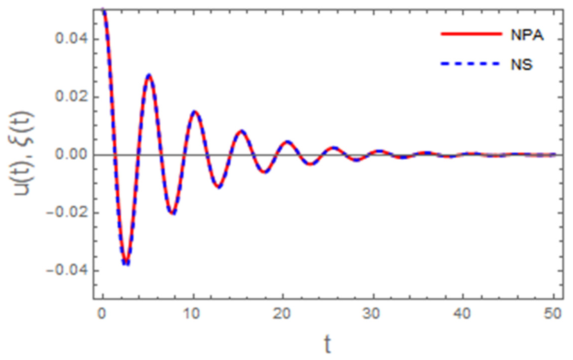
This section analyzes the impact of the inherent physical parameters of the mathematical model on the final analytical expression delineated in Equation (54). The NSs are conducted to exemplify these impacts in a typical system. The resultant solution profiles, illustrating the influence of the controlling parameters, are depicted in Figure 2, Figure 3, Figure 4, Figure 5, Figure 6, Figure 7, Figure 8 and Figure 9.
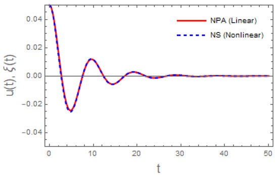
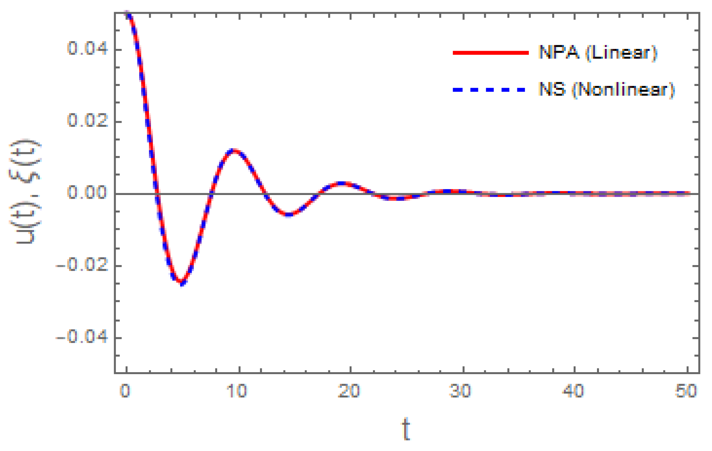
Figure 2 presents a comparative examination of the NS of the nonlinear ODE in Equation (45), represented by the red curve, and its linear equivalent in Equation (54), illustrated by the blue curve. The closeness of the two curves suggests a robust correlation between the nonlinear model and its linearized approximation. The measured variation is negligible, affirming the exceptional precision attained by the NS used. This small disparity indicates that the NS proficiently encapsulates the system’s main behavior and appropriately reflects its fundamental dynamics. The significant correlation between both solutions highlights the reliability and robustness of the numerical methods used to solve complex differential ODEs.
Figure 2.
Comparison of the outcomes of Equations (45) and (54).
The Absolute Error is shown in the following curve.
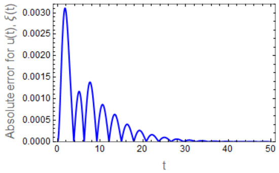
Figure 3 depicts the time-dependent behavior of the Absolute Error between u(t) and ξ(t). At the beginning of the simulation, the error attains a comparatively large magnitude, which can be attributed to the influence of ICs and the dominance of transient nonlinear effects. As time develops, the error displays an oscillatory pattern with decreasing amplitude, reflecting the combined impact of nonlinear interactions and inherent dissipative processes within the system. These oscillations decay rapidly, indicating a progressive convergence between the NS and its approximation. For sufficiently large values of t, the Absolute Error becomes nearly zero and remains insignificant, demonstrating the strong agreement between ξ(t) and u(t). This trend confirms the robustness, accuracy, and numerical stability of the adopted approximation scheme in effectively capturing the system behavior over the investigated time domain.
Figure 3.
The Absolute Error of over time.
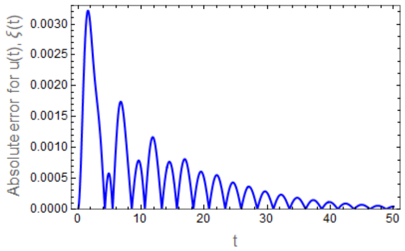
Figure 4 depicts the time evolution of the dimensionless velocity u(t) for various values of the Darcy number β. The results demonstrate that variations in β have a pronounced influence on both the amplitude and the nature of the velocity response. At lower values of β (e.g., β = 0.2), the velocity exhibits larger oscillation amplitudes, indicating weaker resistance offered by the porous medium. As β increases, a significant attenuation in the velocity amplitude is observed throughout the time domain, accompanied by a progressive smoothing of the oscillatory pattern. From a physical perspective, the Darcy number represents the permeability of the porous medium; thus, increasing β enhances the drag force generated by the porous structure, accelerates energy dissipation, and suppresses velocity oscillations. Consequently, the porous medium acts as an effective damping mechanism that stabilizes the unsteady flow as β increases [6,14].
Figure 5 illustrates the influence of the fluid viscosity parameter ζ on the magnitude and temporal evolution of the velocity field. At lower values of ζ, the fluid experiences weaker internal resistance, resulting in higher velocity magnitudes and more pronounced oscillatory behavior. As ζ increases, the peak velocity decreases, and the oscillations decay more rapidly, while the time required to reach velocity extremes becomes longer. This behavior is attributed to enhanced viscous dissipation, where kinetic energy is converted into thermal energy and weakens the flow motion. Therefore, increasing viscosity promotes smoother velocity profiles and enhances flow stability [35,37].
Figure 6 illustrates the time evolution of the dimensionless velocity u(t) for various Weber number values We. At lower Weber numbers, the velocity exhibits larger oscillations during the early stages of motion. However, increasing We leads to a significant reduction in oscillation amplitude and a faster convergence toward the steady state. Since the We represents the ratio of inertial to ST forces, higher values of We reduce the stabilizing influence of ST, leading to enhanced damping and suppression of unsteady velocity fluctuations [38,44].
Figure 7 presents the effect of ρ on the velocity response. Increasing ρ results in larger oscillation amplitudes and noticeable phase shifts, indicating stronger inertial effects. Higher density values allow the fluid to sustain oscillatory motion for a longer duration before dissipation becomes dominant. Although ρ is often associated with flow stabilization, the present results indicate that its role is conditional and depends on the relative balance between inertial and dissipative forces. When inertial effects dominate, increasing ρ enhances oscillatory behavior, whereas in strongly dissipative regimes, density may contribute to flow stabilization [1,7].
Figure 8 shows the impact of the applied MF as H0 on the velocity evolution. Increasing H0 leads to a clear reduction in oscillation amplitude and a faster decay toward equilibrium. This behavior is attributed to the electromagnetic interaction generated by the MF, which opposes the fluid motion and enhances energy dissipation. Consequently, the MF serves as an effective mechanism for damping unsteady motion and stabilizing the flow [5,28].
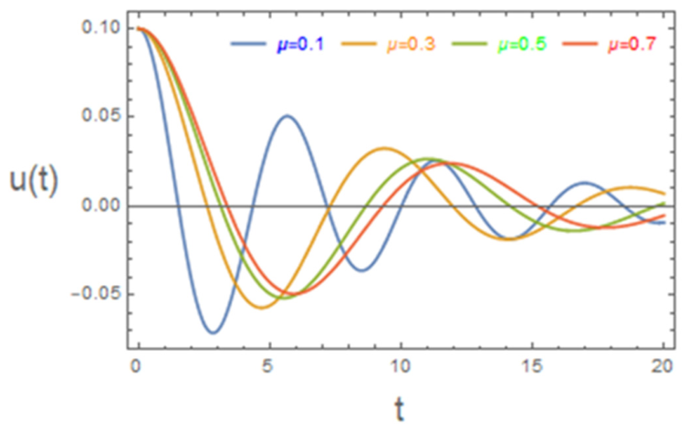
Figure 9 illustrates the influence of magnetic permeability μ on the velocity field. At lower values of μ, the flow exhibits strong oscillations due to weaker electromagnetic interaction. As μ increases, oscillations are significantly damped, and the velocity profile becomes smoother with faster decay. Enhanced magnetic permeability strengthens the coupling between fluid and MF, intensifying the Lorentz force and promoting electromagnetic damping. Hence, magnetic permeability contributes significantly to flow stabilization [29,40].
Generally, the investigated parameters enhance energy dissipation, suppress velocity oscillations, and promote flow stability, with the system dynamics governed by the balance between inertial and dissipative mechanisms.
Figure 4.
Depiction of how the β parameter progresses.
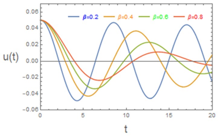
Figure 5.
Portrayal of how the ζ parameter develops.
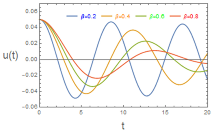
Figure 6.
Portrayal of how the We parameter evolves.
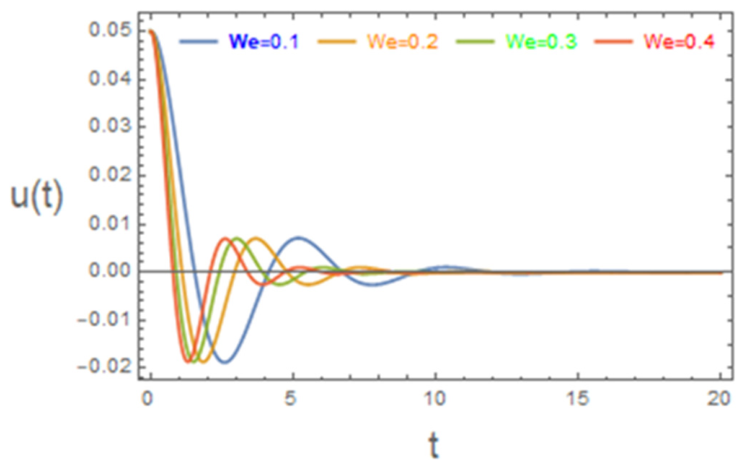
Figure 7.
Depiction of how the ρ parameter changes.
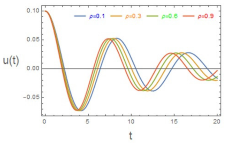
Figure 8.
Depiction of how the parameter evolves.
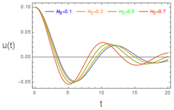
Figure 9.
Depiction of how the μ parameter evolves.
Stability Analysis
The stability findings possess significant practical ramifications for systems dependent on regulated conductive-fluid movement. In MHD pumps, elevated-frequency MFs can stabilize flow, mitigate turbulence, and diminish pressure fluctuations, resulting in more seamless and efficient transport of liquid metals or electrolytes in applications like nuclear reactor cooling and metallurgical processing. In contrast, lower frequencies may improve mixing and flow circulation where agitation is beneficial. In biomedical devices such as magnetic drug-delivery systems, ferrofluid-based microfluidics, and blood-flow control technologies, the capacity to adjust magnetic-field frequency enables meticulous regulation of flow stability, particle transport, and shear stresses, which is essential in ensuring safe and predictable operation. The stability behavior exhibited under periodic magnetic forcing offers crucial insights for enhancing performance, efficiency, and reliability in industrial and biomedical applications.
In what follows, Figure 10, Figure 11, Figure 12, Figure 13, Figure 14, Figure 15, Figure 16 and Figure 17 present the stability configuration of the considered system based on the criterion given in Equation (57) for a system with the following data choices:
In these plots, unstable regions are marked as “unstable,” while stable regions are indicated by the shaded areas labeled “stable.”
Figure 10 presents the system’s stability characteristics in the (k, H0) plane for varying Weber numbers We. The shaded region represents the stable zone, whereas the unshaded region corresponds to the unstable one. It is evident that an increase in the Weber number leads to a shift of the neutral stability boundary downward, leading to an expansion of the stable region over a wide range of wave numbers. As We increases, flow stability can be achieved at lower MF, indicating an enhanced stabilizing effect. Physically, the We represents the ratio of inertial forces to ST forces. In the present configuration, increasing We enhances the dominance of inertial effects that suppress the growth of short-wave interfacial disturbances and delay instability onset. So larger We contributes to stabilizing the system by enlarging the stable domain within the stability map. It is worth noting that the stabilizing role of the We observed here is configuration-dependent and arises from the interaction between inertia, magnetic damping, and interfacial dynamics in the present system [44].
Figure 11 depicts the impact of the density parameter ρ on the stability domain in the (k, H0) plane. Unlike the Weber number case, increasing ρ shifts the stability boundary downward, leading to a pronounced expansion of the stable region. For higher ρ values, stability is achieved at a lower MF over a wide range of wave numbers, indicating enhanced resistance to the growth of instabilities. From a physical perspective, although an increased ρ intensifies inertial effects and may amplify transient oscillations, its role within the linear stability framework is stabilizing. The enhanced inertia slows the growth rate of disturbances, delaying instability onset and enlarging the stable domain. Hence, density contributes to global flow stabilization in terms of stability boundaries, despite its tendency to sustain oscillatory motion in the transient response.
Figure 12 and Figure 13 illustrate the influence of the non-Newtonian parameters N1 and N2 on the system’s stability behavior in the (k, H0) plane. It is evident that increasing either N1 or N2 shifts the neutral stability curves downward, resulting in a pronounced expansion of the stable region and a corresponding reduction in the unstable domain. Moreover, stability is achieved at comparatively lower MF as the non-Newtonian coefficients increase, indicating an enhanced resistance to perturbation growth. Physically, higher values of N1 and N2 intensify nonlinear rheological effects, which introduce additional resistance to deformation and act as effective damping mechanisms. These effects suppress the amplification of disturbances and delay the onset of instability. Consequently, the non-Newtonian properties of both liquids play a significant stabilizing role in governing the global stability behavior of the system [39].
Figure 14 illustrates the influence of the fluid viscosity parameter ζ on the stability characteristics of the system in the (k, H0) plane. The shaded region denotes stable flow, whereas the unshaded region corresponds to instability. The results indicate that an increase in the viscosity parameter ζ causes the neutral stability curve to shift downward, leading to a significant expansion of the stable region and a reduction in the unstable domain. As ζ increases, flow stability can be obtained for reduced values of the MF as H0 over a wide range of wave numbers. In physical terms, higher fluid viscosity enhances viscous dissipation, which suppresses velocity gradients and weakens the growth of perturbations. The increased internal friction serves as an efficient damping mechanism, dissipating kinetic energy more efficiently and delaying the onset of instability. Consequently, fluid viscosity plays a significant stabilizing role in controlling the overall stability behavior of the system. The present findings are in strong agreement with previously reported results [50].
Figure 15 demonstrates the effect of magnetic permeability μ on the stability domain in the (k, H0) plane. The results clearly indicate that variations in μ significantly alter the location of the neutral stability boundary. As the magnetic permeability increases, the stability curve shifts downward, resulting in a noticeable enlargement of the stable region and a corresponding shrinkage of the unstable zone. This behavior implies that stability can be maintained at relatively lower MF when the magnetic permeability is higher. Physically, an increase in μ strengthens the electromagnetic interaction between the fluid motion and the applied MF. This enhancement intensifies the induced electric currents, thereby generating a resistive electromagnetic effect opposing the fluid motion. The resulting electromagnetic damping accelerates the dissipation of kinetic energy and suppresses the amplification of disturbances. Therefore, magnetic permeability acts as a strong stabilizing parameter within the MHD framework of the system. This result is consistent with the findings in [39].
Figure 16 illustrates the influence of the Darcy number β on the stability domain in the (k, H0) plane. It is observed that increasing β shifts the neutral stability curve downward, leading to a noticeable enlargement of the stable region and a corresponding reduction in the unstable domain. Physically, higher values of β correspond to stronger resistance within the porous medium, which enhances energy dissipation and suppresses the growth of disturbances. Consequently, the Darcy number acts as a stabilizing parameter in the present configuration.
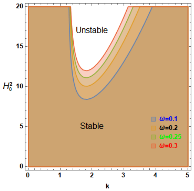
Figure 17 shows the effect of the frequency of the periodic MF ω on the stability characteristics. It is observed that increasing ω shifts the neutral stability curves downward, resulting in an enlargement of the stable region and a corresponding reduction in the unstable domain. This behavior indicates that higher frequencies enhance the stability of the system. Physically, increasing ω introduces rapid temporal oscillations, which act to limit the growth of disturbances by reducing the effective time available for instability development. These oscillations enhance the damping mechanisms and promote energy dissipation within the system. Therefore, the frequency of the periodic MF plays a stabilizing role under the present conditions.
In summary, the stability maps reveal that the system dynamics are governed by a complex interplay between inertial, viscous, rheological, ST, and electromagnetic effects. Parameters associated with enhanced dissipation and resistance mechanisms, including fluid viscosity, MF, magnetic permeability, non-Newtonian coefficients, fluid density, and the Darcy number β, consistently enlarge the stable domain by suppressing the growth of disturbances and delaying instability onset. Moreover, the frequency of the periodic MF ω is shown to exert a stabilizing influence under the present configuration through dynamic modulation, which limits the growth of disturbances and enhances the effective damping mechanisms of the system. Similarly, the Weber number is found to contribute to system stability through its interaction with inertia and magnetic damping. These findings highlight that flow stability arises from a delicate balance among competing physical mechanisms rather than the influence of any single parameter, providing a comprehensive framework for predicting and controlling instability in MHD non-Newtonian flow systems.
Figure 10.
Demonstration of the role of We in shaping the stability do-main.
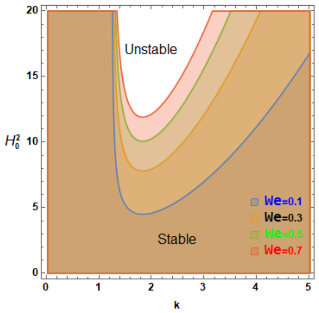
Figure 11.
Validation of the role of ρ in shaping the stability domain.
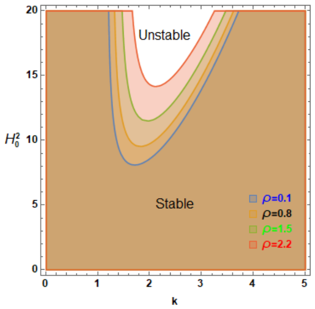
Figure 12.
Display of the role of N1 in shaping the stability domain.
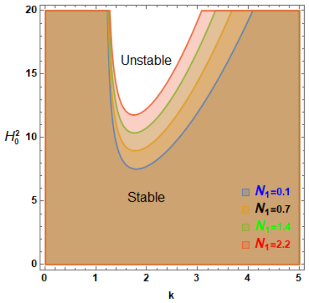
Figure 13.
Display of the role of N2 in shaping the stability domain.
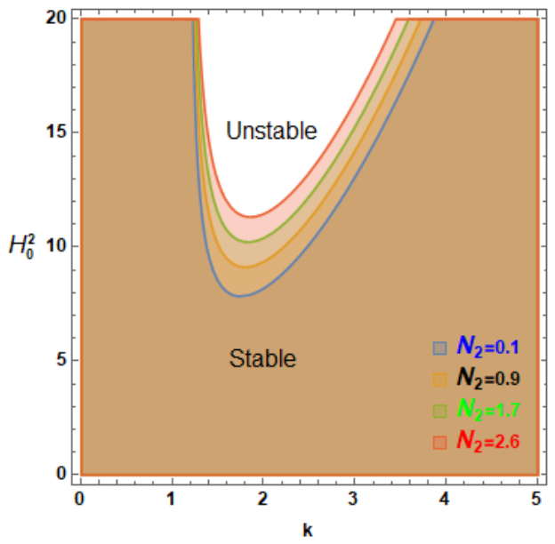
Figure 14.
Display of the role of ζ in shaping the stability domain.
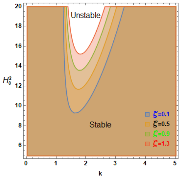
Figure 15.
Demonstration of the role of μ in shaping the stability domain.
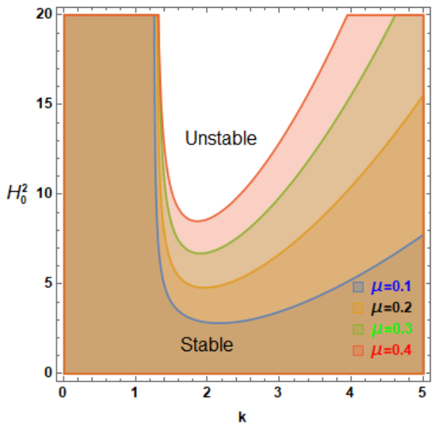
Figure 16.
Display of the role of β in shaping the stability domain.
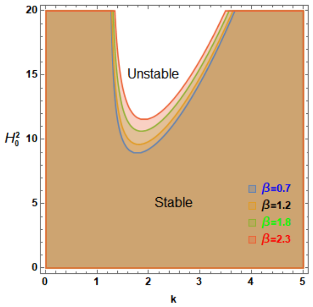
Figure 17.
Display of the role of ω in shaping the stability domain.
7. Uniform MF Case ()
In this scenario, Equation (41) may be expressed as follows:
The nonlinear ODE in Equation (58) can be reformulated as follows:
where
The subsequent analysis investigates the uniform (non-periodic) scenario employing the identical methods to elucidate the overall behavior of the current model for ω≠0. The analytical examination of the resultant linear equations, along with the associated resonance characteristics, stability criteria, and possible chaotic reactions, is conducted to clarify the nonlinear stability attributes of the system. Revisiting the original Equation (59), with coefficients specified in Equation (60), the formulation is augmented to include the uniform terms. The same approach is then utilized to examine the scenario of a uniform MF. Accordingly, the corresponding governing equation for the uniform MF scenario can be expressed as follows:
and the following assumed solution for Equation (46) is considered:
which represents the governing ODE of an equivalent linear damped oscillator, where the coefficient was previously derived in the periodic case and remains unchanged here. The present analysis is therefore focused on determining the value of the natural frequency [48,49,50]:
The standard normal form transformation is employed to eliminate the middle temporal derivative in Equation (61), following the same procedure previously applied in the periodic case. This leads to an undamped linear ODE with a modified natural frequency. The general solution corresponding to Equation (61) is then expressed as follows:
where is evaluated with the aid of MS.
In this formulation, the parameter denotes the effective (dimensionless) damping coefficient evaluated at , whereas incorporates the combined effects of viscous, porous, and viscoelastic dissipation mechanisms. The stability of the interface is guaranteed in the asymptotic sense provided that and , ensuring decay of perturbations over time.
Validation Methodology
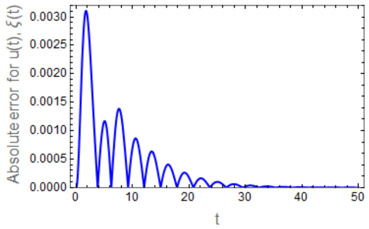
Subsequently, attention is given to the dependence described by Equation (61). This relationship is explored by examining how the MF varies with the axial wavenumber , as demonstrated in the corresponding figures. The NS, together with the analytical approximation derived from Equation (61), is obtained through the following steps: Figure 18 compares the NSs of Equations (58) and (61), represented by the blue and red curves, respectively. The two profiles nearly coincide, with a very small deviation of approximately 0.00137117. This close agreement indicates that both formulations yield consistent results, confirming the accuracy and reliability of the NS used.
Figure 18.
Evaluation and comparison of the outcomes in Equations (58) and (61).
To provide greater clarity, the Absolute Error curve is shown below.
Figure 19 shows the time evolution of the Absolute Error for the state variables, highlighting both transient and steady-state behaviors. The error initially exhibits a sharp peak due to strong transient effects and sensitivity to ICs. It then decreases in a damped oscillatory manner, indicating stable system dynamics and effective energy dissipation. The decay pattern suggests asymptotic convergence, with no signs of instability or irregular fluctuations. At later times, the error approaches zero, confirming high accuracy and strong agreement between the solutions. Overall, the results demonstrate that the proposed system is stable, well-conditioned, and exhibits reliable convergence.
Figure 19.
Depiction of how the Absolute Errors of change with time.
Figure 20, Figure 21, Figure 22 and Figure 23 illustrate the stability domains in the plane. In order to clarify the influence of the governing parameters, each curve is generated by varying a single parameter while keeping all other parameters fixed. The governing equation can be recast into an inequality of the form , subject to the constraint , where the coefficient k is determined by the physical characteristics of the system. The NSs further reveal that the condition may induce instability, indicating the destabilizing role of the MF, which is consistent with previously reported results. As depicted in these figures, the system’s stability characteristics are conveniently represented through the functional relationship between the MF intensity and the surface wavenumber k. The stable configurations correspond to the shaded regions labeled “stability,” whereas the unshaded areas denote unstable regimes.
Figure 20, Figure 21, Figure 22 and Figure 23 provide a comprehensive view of how the Darcy number β, the Ohnesorge number Z, the density ratio ρ, and the magnetic permeability ratio μ affect the stability characteristics in the plane. In all panels, the shaded region denotes stability, whereas the unshaded region indicates instability. The separating curves represent the critical MF required to suppress disturbances of a given wavenumber k.
Figure 20 shows that increasing the density ratio ρ raises the critical MF H02 across the entire wavenumber range, leading to a reduction in the stability region. This behavior reflects enhanced inertial effects associated with larger ρ contrasts, which promote the growth of disturbances, particularly at higher wavenumbers. Hence, ρ acts as a destabilizing parameter [1,6].
Figure 21 reveals that higher values of the Ohnesorge number Z significantly enlarge the stable region. Since Z measures the relative contribution of viscous forces to inertial and ST effects, this confirms that viscosity acts as a strong damping mechanism. The smoothing of the stability boundary at larger Z also indicates reduced sensitivity to variations in k, reflecting a more robust and controlled system response [24,35].
Figure 22 shows that increasing the Darcy number β raises the critical MF , leading to a reduction in the stability region. This indicates that larger β values, associated with porous medium properties, tend to enhance interfacial instability. Physically, the porous structure modifies momentum transport in a way that facilitates disturbance amplification. This destabilizing influence is more evident at intermediate and higher wavenumbers, where the interface becomes increasingly sensitive to perturbations [3,14].
Figure 23 illustrates that increasing the magnetic permeability ratio μ shifts the stability boundary upward, leading to an expansion of the stable region. This indicates that higher magnetic permeability enhances stabilizing magnetic stresses at the interface, making the system more resistant to instability. The stabilizing effect persists over the entire wavenumber range, where short-wavelength disturbances require stronger MFs to become unstable [2,5].
Overall, system stability results from the interplay between viscous Z, porous β, inertial/density ρ, and magnetic μ effects. While ρ and β promote instability by enhancing inertial and porous medium influences, Z and μ contribute to stability through viscous damping and magnetic stress redistribution. These competing mechanisms control the system response.
Figure 20.
Presentation of the role of ρ in shaping the stability region.
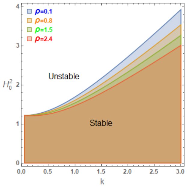
Figure 21.
Presentation of the role of Z in shaping the stability region.
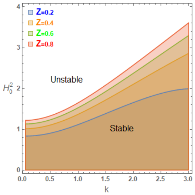
Figure 22.
Presentation of the role of β in shaping the stability region.
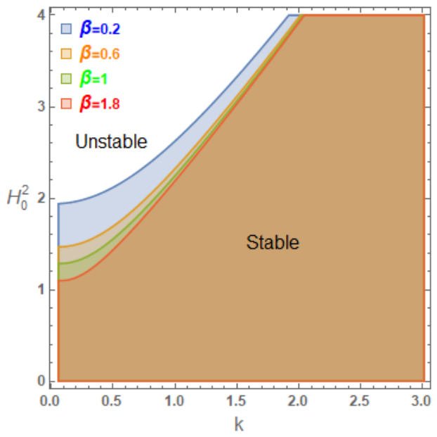
Figure 23.
Presentation of the role of μ in shaping the stability region.
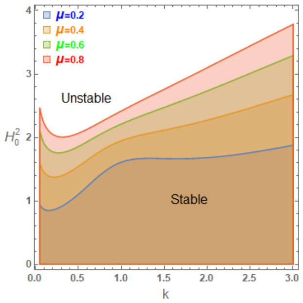
It is important to note that the influence of certain parameters, such as density and Darcy number, differs significantly between periodic and uniform MF configurations. Under periodic magnetic excitation, the time-dependent modulation introduces additional stabilizing mechanisms that can suppress disturbance growth. In contrast, under a uniform MF, such stabilizing modulation is absent, and the same parameters may instead enhance instability due to dominant inertial or resistive effects. This behavior highlights the complex interplay between physical mechanisms and demonstrates that stability characteristics are strongly dependent not only on the governing parameters but also on the nature of the applied MF.
8. Conclusions
This work was motivated by its significance in contemporary material processing and precision engineering, where comprehending and regulating interfacial stability was essential in ensuring dependable performance under diverse operating situations. The interaction between the tangential MF and temporal periodicity produced further mechanisms of mode coupling and enhanced instability. These discoveries highlighted significant deficiencies in nonlinear stability theory and proposed practical applications in flow regulation and the management of conductive fluids. The fluids are considered EPFs at consistent velocities through porous media. The analysis employed the NPA principally based on HFF. The VPT was utilized to streamline mathematical management. The governing PDE equations that characterized the flow are resolved under nonlinear BCs, resulting in a nonlinear characteristic equation for the interface displacement. A non-dimensional methodology was subsequently employed to identify the principal dimensionless physical characteristics affecting the system’s behavior. A set of graphical data was shown to demonstrate the stability features of the system concerning alterations in the pertinent non-dimensional physical parameters. The proposed method is implemented numerically using MS. The analysis examines both uniform and periodic MF. The stability requirements were examined in both scenarios, assessing the impacts of various non-dimensional features. The principal key outcomes can be encapsulated as follows:
- (1)
- The viscosity ζ led to a significant reduction in disturbance growth and improved the nonlinear stability.
- (2)
- Increasing the non-Newtonian parameters (N1 and N2) suppressed oscillation amplitudes and contributed to stabilizing the interface by modifying the effective stress response of the fluids.
- (3)
- As the density ratio ρ increased, it exerted a stabilizing influence in the context of the periodic MF, whereas the opposite effect was observed in the case of a uniform MF.
- (4)
- An increase in MF introduced stronger magnetic damping, shrinking instability regions and promoting stable periodic interfacial motion.
- (5)
- Enhanced conductivity strengthened MHD interactions, resulting in greater energy dissipation and improved system stability.
- (6)
- The Weber number exhibited a stabilizing influence in the present configuration due to the interaction between ST, inertia, and magnetic damping effects.
- (7)
- The wave number determined the size and shape of stable and unstable regions, with certain wavelength ranges being more prone to instability.
- (8)
- The frequency of the periodic MF ω: This parameter controlled the temporal response of the interface and is responsible for the appearance of stable limit cycles and periodic motion.
- (9)
- An increase in porous medium parameters β exerted a stabilizing influence in the context of the periodic MF, whereas the opposite effect was observed in the case of a uniform MF.
There are three primary restrictions in evaluating the NPA. The following constraints may be enumerated:
- i
- The NPA pertains solely to weakly nonlinear oscillators.
- ii
- The initial conditions remain unaltered.
- iii
- To achieve improved accuracy, the initial amplitude must be less than one.
9. Future Work
The nonlinear stability analysis of systems with dual interfaces is crucial in physics and engineering, as it offers a more accurate comprehension of the behavior of layered fluids, plasmas, or multiphase materials under substantial shocks and prolonged operational circumstances. In engineering applications like MHD generators, liquid-metal cooling systems, oil–water transport, and chemical processing, double interfaces may occur between distinct fluid layers, with nonlinear effects influencing the progression of minor perturbations into significant instabilities, mixing, or interface failure. In plasma physics and fusion devices, the nonlinear stability of many interfaces is essential for forecasting confinement quality and mitigating disruptive waves. In biomedical and microfluidic technologies, comprehending nonlinear interfacial behavior enhances the regulation of ferrofluids, targeted drug administration, and lab-on-chip systems where many fluid layers interact under magnetic or EFs. Evaluating nonlinear stability facilitates safer designs, increased efficiency, superior management of transport processes, and more precise predictions of intricate real-world flow behavior, surpassing the constraints of linear theory.
Author Contributions
Conceptualization, A.A., G.M.M. and N.S.G.; Methodology, A.A., G.M.M. and N.S.G.; Software, G.M.M. and N.S.G.; Validation, A.A., G.M.M. and N.S.G.; Formal analysis, A.A., G.M.M. and N.S.G.; Investigation, N.S.G.; Resources, N.S.G.; Data curation, G.M.M. and N.S.G.; Writing—original draft, G.M.M.; Writing—review and editing, N.S.G.; Visualization, N.S.G. All authors have read and agreed to the published version of the manuscript.
Funding
This research received financial support from the Deanship of Graduate Studies and Scientific Research at Qassim University (Grant No. QU-APC-2026).
Data Availability Statement
The original contributions presented in this study are included in the article. Further inquiries can be directed to the corresponding author.
Acknowledgments
The Researchers would like to thank the Deanship of Graduate Studies and Scientific Research at Qassim University (www.qu.edu.sa) for financial support (QU-APC-2026).
Conflicts of Interest
The authors state that they have no known conflicts, financial or otherwise, that could have impacted the outcomes of this research.
Correction Statement
This article has been republished with a minor correction to Acknowledgments. This change does not affect the scientific content of the article.
Abbreviations
| Symbol | Meaning |
| EPF | Eyring–Powell fluid |
| MF | Magnetic field |
| EF | Electric field |
| NPA | Non-perturbative approach |
| HFF | He’s frequency formula |
| RTI | Rayleigh–Taylor instability |
| ST | Surface tension |
| PDE | Partial differential equation |
| HPM | Homotopy perturbation method |
| EHD | Electrohydrodynamics |
| MHD | Magnetohydrodynamics |
| MS | Mathematica Software |
| NS | Numerical solution |
| VPT | Viscous potential theory |
| KHI | Kelvin-Helmholtz instability |
| ODE | Ordinary differential equation |
| MHT | Mass and heat transfer |
| IC | Initial condition |
| Nomenclature | |
| English symbols | |
| A and B | Integration constants |
| We | Weber number |
| Darcy number | |
| Z | Ohnesorge number |
| Initial MF parameter | |
| c.c. | Complex conjugate of preceding terms |
| g | Gravitational acceleration (M ) |
| k | Wavenumber () |
| P | Hydrostatic pressure (Newton/) |
| Initial streaming () | |
| Actual velocity () | |
| () | Cylindrical coordinates |
| Greek symbols | |
| ω | Frequency of periodic MF |
| ζ | Liquid viscosity |
| μj | Magnetic permeability (M L−1 T−1) |
| ρj | Density of fluid (M L−3 ) |
| ξ (x, t) | Interface elevation function (L) |
| φj | Magnetic scalar potentials |
| ψj | Velocity potentials |
| τij | Overall stress tensor |
| ωeq | Equivalent frequency |
| μeq | Equivalent damping |
| Ω | Total frequency |
| δij | Kronecker delta |
Appendix A
The constants appearing in Equations (23) and (24) may be formulated as
and
The constants appearing in Equation (33) can be written as
and
References
- Cowley, M.D.; Rosenensweig, R.E. The interfacial stability of a ferromagnetic fluid. J. Fluid Mech. 1967, 30, 671–688. [Google Scholar] [CrossRef] [Scilit]
- Rosensweig, R.E. Ferrohydrodynamics; Cambridge University Press: Cambridge, UK, 1985. [Google Scholar]
- Malik, S.K.; Singh, M. Modulation in magnetic fluids. Q. Appl. Math. 1985, 43, 57–64. [Google Scholar] [CrossRef] [Scilit]
- Akbar, N.S.; Nadeem, S. Endoscopic effects on peristaltic flow of a nanofluid. Appl. Nanosci. 2011, 56, 761. [Google Scholar] [CrossRef] [Scilit]
- Melcher, J.R. Field Coupled Surface Waves; M.I.T. Press: Cambridge, MA, USA, 1963. [Google Scholar]
- Zelazo, R.E.; Melcher, J.R. Dynamics and stability of ferrofluids: Surface interactions. J. Fluid Mech. 1969, 39, 1–24. [Google Scholar] [CrossRef] [Scilit]
- Drazin, P.G.; Reid, W.H. Hydrodynamic Stability; Cambridge University Press: Cambridge, UK, 2004. [Google Scholar]
- Hemamalini, P.T. Kelvin-Helmholtz instability of superposed ferrofluids in the presence of periodic tangential magnetic field. Int. J. Mech. Eng. 2018, 9, 674–685. [Google Scholar]
- Afonso, A.M.; Alves, M.A.; Pinho, F.T. Electro-osmotic flow of viscoelastic fluids. J. Non-Newton. Fluid Mech. 2009, 159, 50–63. [Google Scholar] [CrossRef] [Scilit]
- Khan, U.; Zaib, A.; Ishak, A. Magnetic field effect on Sisko fluid flow containing gold nanoparticles through a Porous curved surface in the presence of radiation and partial slip. Mathematics 2021, 9, 921. [Google Scholar] [CrossRef] [Scilit]
- Waini, I.; Ishak, A.; Pop, I. Eyring–Powell fluid flow past a shrinking sheet: Effect of Magnetohydrodynamic (MHD) and Joule heating. J. Adv. Res. Fluid Mech. Therm. Sci. 2024, 116, 64–77. [Google Scholar] [CrossRef] [Scilit]
- Khan, Z.; Rasheed, H.U.; Abbas, T.; Khan, W.; Khan, I.; Baleanu, D.; Nisar, K.S. Analysis of Eyring–Powell fluid flow used as a coating material for wire with variable viscosity effect along with thermal radiation and joule heating. Crystals 2020, 10, 168. [Google Scholar] [CrossRef] [Scilit]
- Riaz, A.; Ellahi, R.; Sait, S.M. Role of hybrid nanoparticles in thermal performance of peristaltic flow of Eyring–Powell fluid model. J. Therm. Anal. Calorim. 2021, 143, 1021–1035. [Google Scholar] [CrossRef] [Scilit]
- Nadeem, S.; Mushtaq, A.; Alzabut, J.; Ghazwani, H.A.; Eldin, S.M. The flow of an Eyring Powell nanofluid in a porous peristaltic channel through a porous medium. Sci. Rep. 2023, 13, 9694. [Google Scholar] [CrossRef] [Scilit] [PubMed]
- Karthik, S.; Iranian, D.; Alhazmi, H.; Khan, I.; Singh, A.; Khan, A.I. Double diffusive on Powell Eyring fluid flow by mixed convection from an exponential stretching surface with variable viscosity/thermal conductivity. Case Stud. Therm. Eng. 2024, 55, 104091. [Google Scholar] [CrossRef] [Scilit]
- Abbas, W.; Megahed, A.M.; Emam, M.S.; Sadek, H.M.H. MHD dissipative Powell-Eyring fluid flow due to a stretching sheet with convective boundary conditions and slip velocity. Sci. Rep. 2023, 13, 15674. [Google Scholar] [CrossRef] [Scilit]
- Sarkar, A.; Mondal, H.; Nandkeolyar, R. Powell-Eyring fluid flow over a stretching surface with variable properties. J. Nanofluids 2023, 12, 47–54. [Google Scholar] [CrossRef] [Scilit]
- Nadeem, S.; Ishtiaq, B.; Akkurt, N.; Eldin, S.M. Swirling flow analysis of Eyring–Powell fluid between coaxial disks with variable property. J. Comput. Des. Eng. 2023, 10, 632–640. [Google Scholar] [CrossRef] [Scilit]
- Manimegalai, K.; Zephania, C.F.S.; Bera, P.K.; PBera Das, S.K.; Sil, T. Study of strongly nonlinear oscillators using the Aboodh transform and the homotopy perturbation method. Eur. Phys. J. Plus 2019, 134, 462. [Google Scholar] [CrossRef] [Scilit]
- Wang, J. The extended Rayleigh-Ritz method for an analysis of nonlinear vibrations. Mech. Adv. Mater. Struct. 2022, 29, 3281–3284. [Google Scholar] [CrossRef] [Scilit]
- Shi, B.; Yang, J.; Wang, J. Forced vibration analysis of multi-degree-of-freedom nonlinear systems with the extended Galerkin method. Mech. Adv. Mater. Struct. 2023, 30, 794–802. [Google Scholar] [CrossRef] [Scilit]
- Abu-As’ad, A.; Asad, J. Power series approach to nonlinear oscillators. J. Low Freq. Noise Vib. Act. Control. 2024, 43, 220–238. [Google Scholar] [CrossRef] [Scilit]
- Ismail, G.M.; Abu-Zinadah, H. Analytic approximations to non-linear third order jerk equations via modified global error minimization method. J. King Saud. Univ. 2021, 33, 101219. [Google Scholar] [CrossRef] [Scilit]
- He, J.-H. Some asymptotic methods for strongly nonlinear equations. Int. J. Mod. Phys. B 2006, 20, 1141–1199. [Google Scholar] [CrossRef] [Scilit]
- He, J.-H. The simpler, the better: Analytical methods for nonlinear oscillators and fractional oscillators. J. Low Freq. Noise Vib. Act. Control. 2019, 38, 1252–1260. [Google Scholar] [CrossRef] [Scilit]
- Qie, N.; Hou, W.F.; He, J.-H. The fastest insight into the large amplitude vibration of a string. Rep. Mech. Eng. 2021, 2, 1–5. [Google Scholar] [CrossRef] [Scilit]
- He, J.-H.; Yang, Q.; He, C.; Khan, Y. A simple frequency formulation for the tangent oscillator. Axioms 2021, 10, 320. [Google Scholar] [CrossRef] [Scilit]
- Moatimid, G.M.; Sayed, A. Nonlinear EHD stability of a cylindrical interface separating two Rivlin-Ericksen fluids: A Novel analysis. Chin. J. Phys. 2024, 87, 379–397. [Google Scholar] [CrossRef] [Scilit]
- Saville, D.A. Electrohydrodynamics: The Taylor–Melcher leaky dielectric model. Annu. Rev. Fluid Mech. 2003, 29, 27–64. [Google Scholar] [CrossRef] [Scilit]
- Moatimid, G.M.; Mohamed, Y.M. Nonlinear electro-rheological instability of two moving cylindrical fluids: An innovative approach. Phys. Fluids 2024, 36, 024110. [Google Scholar] [CrossRef] [Scilit]
- Yuan, G.; Song, J.; Yang, Y.; Ni, B.; Yang, D.; Xue, Y. Experimental study on icebreaking mechanism and failure modes of submerged high-pressure water jets. Ocean. Eng. 2025, 323, 120586. [Google Scholar] [CrossRef] [Scilit]
- Yang, J.; Fan, P.; Wang, M.; Li, J.; Qian, Q. Perturbation-induced delayed shear creep instability in rock Joints: A nonlinear model based on irreversible deformation. Int. J. Rock Mech. Min. Sci. 2025, 195, 106289. [Google Scholar] [CrossRef] [Scilit]
- Xia, Y.; Zhang, B.; Tao, C.; Wang, L. Fully nonlinear simulation of the hydrodynamic performance of a submerged cylindrical wave energy converter in the presence of current. J. Mar. Sci. Eng. 2025, 123, 1763. [Google Scholar] [CrossRef] [Scilit]
- Ye, L.; She, H.; Sun, C.; Wang, X.; Liu, C.; Shi, C. A mass-flux-vector-based design for self-angled slot arrangements enhancing leading edge showerhead cooling. Int. Commun. Heat Mass Transf. 2026, 172, 110305. [Google Scholar] [CrossRef] [Scilit]
- Lamb, H. Hydrodynamics; Cambridge University Press: Cambridge, UK, 1932. [Google Scholar]
- Batchelor, G.K. An Introduction to Fluid Dynamics; Cambridge University Press: Cambridge, UK, 1997. [Google Scholar]
- Funada, T.; Joseph, D.D. Viscous potential flow analysis of Kelvin–Helmholtz instability in a channel. J. Fluid Mech. 2001, 445, 263–283. [Google Scholar] [CrossRef] [Scilit]
- Funada, T.; Joseph, D.D. Viscous potential flow analysis of capillary instability. Int. J. Multiph. Flow 2002, 28, 1459–1478. [Google Scholar] [CrossRef] [Scilit]
- Moatimid, G.M.; Mohamed, Y.M. A novel methodology in analyzing nonlinear stability of two electrified viscoelastic liquids. Chin. J. Phys. 2024, 89, 679–706. [Google Scholar] [CrossRef] [Scilit]
- El-Sayed, M.F.; El-Dabe, N.T.M. Nonlinear electrohydrodynamic Kelvin–Helmholtz instability of viscoelastic fluid layers. ZAMP 2012, 63, 1027–1050. [Google Scholar]
- Moatimid, G.M.; Mostafa, D.M.; Zekry, M.H. A new methodology in evaluating nonlinear Electrohydrodynamic azimuthal stability between two dusty viscous fluids. Chin. J. Phys. 2024, 90, 134–154. [Google Scholar] [CrossRef] [Scilit]
- Ibrahim, W.; Lamesse, T. Powell-Eyring nanofluid analysis with finite element method when past stretching sheet with convective heating and passive control of nanoparticle. Int. J. Thermofluids 2023, 19, 100388. [Google Scholar] [CrossRef] [Scilit]
- Moatimid, G.M.; Mostafa, D.M. Nonlinear stability of two superimposed electrified dusty fluids of type Rivlin-Ericksen: Non-perturbative approach. Partial. Differ. Equ. Appl. Math. 2024, 10, 100745. [Google Scholar] [CrossRef] [Scilit]
- Chandrasekhar, S. Hydrodynamic and Hydromagnetic Stability; Dover Publications: New York, NY, USA, 1961. [Google Scholar]
- Caughey, T.K. Equivalent linearization techniques. J. Acoust. Soc. Am. 1963, 35, 1706–1711. [Google Scholar] [CrossRef] [Scilit]
- Iwan, W.D. On defining equivalent systems for certain ordinary nonlinear differential equations. Int. J. Non-Linear Mech. 1969, 4, 325–334. [Google Scholar] [CrossRef] [Scilit]
- Spanos, P.T.D.; Iwan, W.D. On the existence and uniqueness of solutions generated by equivalent linearization. Int. J. Non-Linear Mech. 1979, 13, 71–78. [Google Scholar] [CrossRef] [Scilit]
- El-Dib, Y.O. Stability analysis of a time-delayed van der Pol–Helmholtz–Duffing oscillator in fractal space with a non-perturbative approach. Commun. Theor. Phys. 2024, 76, 045003. [Google Scholar] [CrossRef] [Scilit]
- El-Dib, Y.O. The masking technique for forced nonlinear oscillator stability behavior analysis using the non-perturbative approach. J. Low Freq. Noise Vib. Act. Control. 2024, 43, 1481–1497. [Google Scholar] [CrossRef] [Scilit]
- El-Dib, Y.O.; Al-Ghamdi, H. Renormalization method for variable stiffness in fractal DOF nonlinear parametric oscillators. J. Vib. Eng. Technol. 2025, 13, 550. [Google Scholar] [CrossRef] [Scilit]
Disclaimer/Publisher’s Note: The statements, opinions and data contained in all publications are solely those of the individual author(s) and contributor(s) and not of MDPI and/or the editor(s). MDPI and/or the editor(s) disclaim responsibility for any injury to people or property resulting from any ideas, methods, instructions or products referred to in the content. |
© 2026 by the authors. Licensee MDPI, Basel, Switzerland. This article is an open access article distributed under the terms and conditions of the Creative Commons Attribution (CC BY) license.