A New Subclass of Analytic Functions Involving the ($\mathfrak{p},\mathfrak{q}$)-Derivative and Applications to ($\mathfrak{p},\mathfrak{q}$)-Poisson Distribution Series

Abstract

In this paper, we introduce and investigate a new subclass ${\mathcal{A}}_{\mathfrak{p},\mathfrak{q}}(\lambda ,\delta ,\eta )$ of analytic functions defined by the $(\mathfrak{p},\mathfrak{q})$-derivative in the setting of Geometric Function Theory. This class extends the classical subclass $\mathcal{G}(\lambda ,\delta ,\eta )$ and reduces to it when the parameters $\mathfrak{p}$ and $\mathfrak{q}$ tend to $1^{-}$. By means of coefficient estimates, we obtain a sufficient condition for the general class and a necessary and sufficient condition for the corresponding negative-coefficient subclass. These results are then applied to the $(\mathfrak{p},\mathfrak{q})$-Poisson distribution series and to a related linear operator. The graphical analysis included in the final section illustrates the geometric behavior of the introduced functions and highlights the effects of the parameters.

1. Introduction and Preliminaries

Let $\mathcal{A}$ denote the class of analytic functions f in the open unit disk $\mathbb{U}=\{z\in \mathbb{C}:|z|<1\}$, normalized by $f\left(0\right)=0$ and $f\prime \left(0\right)=1$, and having the form

$$f\left(z\right)=z+{\displaystyle \sum _{\ell =2}^{\infty }}{a}_{\ell }{z}^{\ell }.$$

(1)

We denote by $\mathcal{S}$ the subclass of $\mathcal{A}$ consisting of functions that are univalent in $\mathbb{U}$. Furthermore, let $\mathcal{T}$ be the subclass of functions $f\in \mathcal{A}$ of the form

$$f\left(z\right)=z-{\displaystyle \sum _{\ell =2}^{\infty }}\left|a_{\ell }\right|z^{\ell }.$$

(2)

A well-known subclass of $\mathcal{A}$ is the class $\mathcal{G}(\lambda ,\delta ,\eta )$, which was studied by Wang et al. [1]. For $\lambda ,\delta >0$ and $0\le \eta <\lambda +\delta \le 1$, it is defined by

$$\mathcal{G}(\lambda ,\delta ,\eta )=\left\{f\in \mathcal{A}:\Re \left(\lambda {\displaystyle \frac{f\left(z\right)}{z}}+\delta f\prime \left(z\right)\right)>\eta ,z\in \mathbb{U}\right\}.$$

In 1990, Ismail et al. [2] introduced the use of $\mathfrak{q}$-calculus into the theory of analytic univalent functions by considering a family of complex-valued functions that are analytic in the open unit disk $\mathbb{U}$ and satisfy suitable normalization conditions. More precisely, these functions are normalized by $f\left(0\right)=0$ and $f\prime \left(0\right)=1$, and they fulfill the inequality $\left|f\right(\mathfrak{q}z\left)\right|\le \left|f\right(z\left)\right|$ for all $z\in \mathbb{U}$ and for each $\mathfrak{q}$ with $0<\mathfrak{q}<1$.

Inspired by this pioneering work, a growing body of research has explored the interaction between analytic univalent function theory and $\mathfrak{q}$-calculus; see, for example ref. [3].

The $(\mathfrak{p},\mathfrak{q})$-calculus was first introduced in the context of quantum algebras by Chakrabarti and Jagannathan [4]. Throughout this paper, we adopt the standard notation of $(\mathfrak{p},\mathfrak{q})$-calculus with $0<\mathfrak{q}<\mathfrak{p}<1$. For any non-negative integer ℓ, the $(\mathfrak{p},\mathfrak{q})$-integer ${[\ell ]}_{\mathfrak{p},\mathfrak{q}}$ is defined by

$${[\ell ]}_{\mathfrak{p},\mathfrak{q}}={\displaystyle \frac{{\mathfrak{p}}^{\ell }-{\mathfrak{q}}^{\ell }}{\mathfrak{p}-\mathfrak{q}}},{\left[0\right]}_{\mathfrak{p},\mathfrak{q}}=0,{\left[1\right]}_{\mathfrak{p},\mathfrak{q}}=1.$$

In the limiting case $\mathfrak{p}\to 1^{-}$, one obtains the $\mathfrak{q}$-integer

$${[\ell ]}_{\mathfrak{q}}={\displaystyle \frac{1-{\mathfrak{q}}^{\ell }}{1-\mathfrak{q}}},{\left[0\right]}_{\mathfrak{q}}=0,{\left[1\right]}_{\mathfrak{q}}=1,$$

and it is clear that ${lim}_{\mathfrak{q}\to 1^{-}}{[\ell ]}_{\mathfrak{q}}=\ell$.

The $(\mathfrak{p},\mathfrak{q})$-analogue of the factorial function is defined by

$${[\ell ]}_{\mathfrak{p},\mathfrak{q}}!={\left[1\right]}_{\mathfrak{p},\mathfrak{q}}{\left[2\right]}_{\mathfrak{p},\mathfrak{q}} \dots {[\ell ]}_{\mathfrak{p},\mathfrak{q}},{\left[0\right]}_{\mathfrak{p},\mathfrak{q}}!=1,$$

with the limiting relations

$$\underset{\mathfrak{p}\to 1^{-}}{lim}{[\ell ]}_{\mathfrak{p},\mathfrak{q}}!={[\ell ]}_{\mathfrak{q}}!,\underset{\mathfrak{q}\to 1^{-}}{lim}{[\ell ]}_{\mathfrak{q}}!=\ell !.$$

The $(\mathfrak{p},\mathfrak{q})$-derivative of a function f analytic in $\mathbb{U}$ is defined by

$$D_{\mathfrak{p},\mathfrak{q}}f\left(z\right)=\left\{\begin{array}{cc}{\displaystyle \frac{f\left(\mathfrak{p}z\right)-f\left(\mathfrak{q}z\right)}{(\mathfrak{p}-\mathfrak{q})z}},\hfill & z\ne 0,\hfill \\ f\prime \left(0\right),\hfill & z=0,\hfill \end{array}\right.$$

(3)

and it satisfies

$$\underset{\mathfrak{p}\to 1^{-}}{lim}{D}_{\mathfrak{p},\mathfrak{q}}f\left(z\right)=D_{\mathfrak{q}}f\left(z\right),\underset{\mathfrak{q}\to 1^{-}}{lim}{D}_{\mathfrak{q}}f\left(z\right) = f\prime \left(z\right).$$

Further details on $\mathfrak{q}$- and $(\mathfrak{p},\mathfrak{q})$-calculus can be found in [3,5,6,7].

For a function f of the form (1), we have the series representation

$$D_{\mathfrak{p},\mathfrak{q}}f\left(z\right)=1+{\displaystyle \sum _{\ell =2}^{\infty }}{[\ell ]}_{\mathfrak{p},\mathfrak{q}}{a}_{\ell }{z}^{\ell -1}.$$

(4)

For $0<\mathfrak{q}<\mathfrak{p}<1$ and $\lambda ,\delta >0$, $0\le \eta <\lambda +\delta \le 1$, we define the class ${\mathcal{A}}_{\mathfrak{p},\mathfrak{q}}(\lambda ,\delta ,\eta )$ by

$${\mathcal{A}}_{\mathfrak{p},\mathfrak{q}}(\lambda ,\delta ,\eta )=\left\{f\in \mathcal{A}:\Re \left(\lambda {\displaystyle \frac{f\left(z\right)}{z}}+\delta D_{\mathfrak{p},\mathfrak{q}}f\left(z\right)\right)>\eta ,z\in \mathbb{U}\right\}.$$

We also write

$$\mathcal{T}{\mathcal{A}}_{\mathfrak{p},\mathfrak{q}}(\lambda ,\delta ,\eta )=\mathcal{T}\cap {\mathcal{A}}_{\mathfrak{p},\mathfrak{q}}(\lambda ,\delta ,\eta ).$$

It is clear that

$${\mathcal{A}}_{\mathfrak{p},\mathfrak{q}}(\lambda ,\delta ,\eta )=\mathcal{G}(\lambda ,\delta ,\eta )\mathrm{as}\mathfrak{p},\mathfrak{q}\to 1^{-}.$$

The combination of the classical class $\mathcal{G}(\lambda ,\delta ,\eta )$ with the $(\mathfrak{p},\mathfrak{q})$-derivative is of interest because it simultaneously preserves the geometric interpretation of the original real-part condition and introduces two deformation parameters into the coefficient structure. This allows the classical inclusion criteria to be refined through quantum-calculus parameters and provides a flexible bridge between known analytic-function classes, their $\mathfrak{q}$-analogues, and the limiting classical case.

The purpose of the present work is not only to replace the classical derivative by the $(\mathfrak{p},\mathfrak{q})$-derivative, but also to examine how the two-parameter structure affects coefficient criteria for analytic functions with general and negative Taylor coefficients, and how these criteria can be applied to Poisson-type distribution series and the associated linear operator. In this sense, the paper provides a unified framework in which sharp coefficient estimates, necessary and sufficient conditions for the negative-coefficient case, limiting reductions to known classes, and graphical interpretations of the resulting mappings are treated together.

The Poisson distribution series has recently attracted considerable interest in Geometric Function Theory [8,9,10,11,12,13,14,15,16]. In this direction, both the $\mathfrak{q}$-Poisson and $(\mathfrak{p},\mathfrak{q})$-Poisson distribution series have been introduced and studied by several authors, and their connections with subclasses of analytic and harmonic univalent functions have been examined [17].

A random variable x is said to have a $(\mathfrak{p},\mathfrak{q})$-Poisson distribution if it takes the values $0,1,2,\dots$ with probabilities

$${\displaystyle \frac{r^{\ell }}{{[\ell ]}_{\mathfrak{p},\mathfrak{q}}!}}{e}_{\mathfrak{p},\mathfrak{q}}^{-r},\ell =0,1,2,\dots ,$$

where $r>0$ and

$$e_{\mathfrak{p},\mathfrak{q}}^x={\displaystyle \sum _{\ell =0}^{\infty }}{\displaystyle \frac{x^{\ell }}{{[\ell ]}_{\mathfrak{p},\mathfrak{q}}!}}$$

(5)

denotes the $(\mathfrak{p},\mathfrak{q})$-exponential function.

The associated $(\mathfrak{p},\mathfrak{q})$-Poisson distribution series is given by

$${\mathcal{P}}_{\mathfrak{p},\mathfrak{q}}^r\left(z\right)=z+{\displaystyle \sum _{\ell =2}^{\infty }}{\displaystyle \frac{r^{\ell -1}{e}_{\mathfrak{p},\mathfrak{q}}^{-r}}{{[\ell -1]}_{\mathfrak{p},\mathfrak{q}}!}}{z}^{\ell },z\in \mathbb{U},$$

(6)

which has an infinite radius of convergence. Its negative-coefficient counterpart is defined by

$$\mathcal{T}{\mathcal{P}}_{\mathfrak{p},\mathfrak{q}}^r\left(z\right)=z-{\displaystyle \sum _{\ell =2}^{\infty }}{\displaystyle \frac{r^{\ell -1}{e}_{\mathfrak{p},\mathfrak{q}}^{-r}}{{[\ell -1]}_{\mathfrak{p},\mathfrak{q}}!}}{z}^{\ell },z\in \mathbb{U}.$$

(7)

Clearly,

$${\mathcal{P}}_{\mathfrak{p},\mathfrak{q}}^r\in \mathcal{A}\mathrm{and}\mathcal{T}{\mathcal{P}}_{\mathfrak{p},\mathfrak{q}}^r\in \mathcal{T}.$$

Based on the $(\mathfrak{p},\mathfrak{q})$-Poisson distribution series, we introduce the following linear operator:

$$\begin{array}{cc}\hfill N_{\mathfrak{p},\mathfrak{q}}^{r,\mu }\left(z\right)& =(1-\mu ){\mathcal{P}}_{\mathfrak{p},\mathfrak{q}}^r\left(z\right)+\mu z{D}_{\mathfrak{p},\mathfrak{q}}{\mathcal{P}}_{\mathfrak{p},\mathfrak{q}}^r\left(z\right)\hfill \\ \hfill & =z+{\displaystyle \sum _{\ell =2}^{\infty }}{\displaystyle \frac{r^{\ell -1}{e}_{\mathfrak{p},\mathfrak{q}}^{-r}}{{[\ell -1]}_{\mathfrak{p},\mathfrak{q}}!}}\left[1+\mu \left({[\ell ]}_{\mathfrak{p},\mathfrak{q}}-1\right)\right]z^{\ell },\hfill \end{array}$$

(8)

where $r>0$ and $0\le \mu \le 1$.

Next, we define the associated negative-coefficient operator by

$$\mathcal{T}{N}_{\mathfrak{p},\mathfrak{q}}^{r,\mu }\left(z\right):=2z-N_{\mathfrak{p},\mathfrak{q}}^{r,\mu }\left(z\right)=z-{\displaystyle \sum _{\ell =2}^{\infty }}{\displaystyle \frac{r^{\ell -1}{e}_{\mathfrak{p},\mathfrak{q}}^{-r}}{{[\ell -1]}_{\mathfrak{p},\mathfrak{q}}!}}\left(1-\mu +\mu {[\ell ]}_{\mathfrak{p},\mathfrak{q}}\right)z^{\ell }.$$

We also define the convolution (Hadamard product) associated with ${\mathcal{P}}_{\mathfrak{p},\mathfrak{q}}^r$ by

$$P_{\mathfrak{p},\mathfrak{q}}^r\left(f\right)\left(z\right):={\mathcal{P}}_{\mathfrak{p},\mathfrak{q}}^r\left(z\right)\ast f\left(z\right)=z+{\displaystyle \sum _{\ell =2}^{\infty }}{\displaystyle \frac{r^{\ell -1}{e}_{\mathfrak{p},\mathfrak{q}}^{-r}}{{[\ell -1]}_{\mathfrak{p},\mathfrak{q}}!}}{a}_{\ell }{z}^{\ell },$$

where $f\left(z\right)=z+{\sum }_{\ell =2}^{\infty }{a}_{\ell }{z}^{\ell }\in \mathcal{A}$.

The main purpose of this paper is to study the membership properties of the $(\mathfrak{p},\mathfrak{q})$-Poisson distribution series and the linear operator $N_{\mathfrak{p},\mathfrak{q}}^{r,\mu }\left(z\right)$ in the class ${\mathcal{A}}_{\mathfrak{p},\mathfrak{q}}(\lambda ,\delta ,\eta )$. In addition, we obtain necessary and sufficient conditions for the associated negative-coefficient operator $\mathcal{T}{N}_{\mathfrak{p},\mathfrak{q}}^{r,\mu }\left(z\right)$ to belong to the class $\mathcal{T}{\mathcal{A}}_{\mathfrak{p},\mathfrak{q}}(\lambda ,\delta ,\eta )$. To achieve these goals, we first derive sharp coefficient criteria and then apply them to the above series and operators. Several known results are recovered as special cases when the parameters approach their classical limits.

2. Coefficient Conditions for the Class ${\mathcal{A}}_{\mathfrak{p},\mathfrak{q}}(\mathit{\lambda },\mathit{\delta },\mathit{\eta })$

This section is devoted to the derivation of coefficient conditions for the class ${\mathcal{A}}_{\mathfrak{p},\mathfrak{q}}(\lambda ,\delta ,\eta )$ and the class $\mathcal{T}{\mathcal{A}}_{\mathfrak{p},\mathfrak{q}}(\lambda ,\delta ,\eta )$. Such conditions are fundamental in the study of analytic functions, as they allow one to characterize membership properties in terms of the Taylor coefficients. The results obtained here will be used in the subsequent section to investigate applications involving Poisson-type distribution series.

We first establish a sufficient coefficient condition for functions to belong to the class ${\mathcal{A}}_{\mathfrak{p},\mathfrak{q}}(\lambda ,\delta ,\eta )$.

Theorem 1.

Let $f\in \mathcal{A}$ be of the form (1). If

$${\displaystyle \sum _{\ell =2}^{\infty }}\left(\lambda +\delta {[\ell ]}_{\mathfrak{p},\mathfrak{q}}\right)\left|a_{\ell }\right|\le \lambda +\delta -\eta ,$$

(9)

where $\lambda ,\delta >0$ and $0\le \eta <\lambda +\delta \le 1$, then $f\in {\mathcal{A}}_{\mathfrak{p},\mathfrak{q}}(\lambda ,\delta ,\eta )$.

Proof. 

The condition $\Re w>\eta$ is equivalent to $|1-\eta +w|>|1+\eta -w|$. Therefore, it is sufficient to show that

$$\left|1-\eta +\lambda {\displaystyle \frac{f\left(z\right)}{z}}+\delta D_{\mathfrak{p},\mathfrak{q}}f\left(z\right)\right|-\left|1+\eta -\lambda {\displaystyle \frac{f\left(z\right)}{z}}-\delta D_{\mathfrak{p},\mathfrak{q}}f\left(z\right)\right|>0,z\in \mathbb{U}.$$

(10)

Using the series expansion (4) of $D_{\mathfrak{p},\mathfrak{q}}f\left(z\right)$, we obtain

$$1-\eta +\lambda {\displaystyle \frac{f\left(z\right)}{z}}+\delta D_{\mathfrak{p},\mathfrak{q}}f\left(z\right)=1-\eta +\lambda +\delta +{\displaystyle \sum _{\ell =2}^{\infty }}\left(\lambda +\delta {[\ell ]}_{\mathfrak{p},\mathfrak{q}}\right)a_{\ell }{z}^{\ell -1}.$$

Substituting this expression into (10) and applying the triangle inequality, we arrive at

$$\begin{array}{cc}\hfill & \left|1-\eta +\lambda +\delta +{\displaystyle \sum _{\ell =2}^{\infty }}\left(\lambda +\delta {[\ell ]}_{\mathfrak{p},\mathfrak{q}}\right)a_{\ell }{z}^{\ell -1}\right|\hfill \\ \hfill & -\left|1+\eta -\lambda -\delta -{\displaystyle \sum _{\ell =2}^{\infty }}\left(\lambda +\delta {[\ell ]}_{\mathfrak{p},\mathfrak{q}}\right)a_{\ell }{z}^{\ell -1}\right|\hfill \\ \hfill & \ge 2(\lambda +\delta -\eta )-2{\displaystyle \sum _{\ell =2}^{\infty }}\left(\lambda +\delta {[\ell ]}_{\mathfrak{p},\mathfrak{q}}\right)|a_{\ell }{\left|\right|z|}^{\ell -1}\hfill \\ \hfill & >2(\lambda +\delta -\eta )-2{\displaystyle \sum _{\ell =2}^{\infty }}\left(\lambda +\delta {[\ell ]}_{\mathfrak{p},\mathfrak{q}}\right)\left|a_{\ell }\right|.\hfill \end{array}$$

By assumption (9), the last expression is non-negative. Hence, inequality (10) holds for all $z\in \mathbb{U}$, which implies that $f\in {\mathcal{A}}_{\mathfrak{p},\mathfrak{q}}(\lambda ,\delta ,\eta )$. □

Remark 1.

The coefficient condition in Theorem 1 is sufficient but not necessary for the full class of analytic functions. In the general case, no sign restriction is imposed on the Taylor coefficients, and the triangle inequalities used in the proof may be strict because of cancellations among complex coefficients. Therefore, membership in the class does not necessarily force the coefficient inequality in Theorem 1. The negative-coefficient subclass treated in Theorem 2 is different, since the fixed sign pattern permits an exact necessary and sufficient characterization.

We next obtain a necessary and sufficient coefficient condition for functions in the subclass $\mathcal{T}{\mathcal{A}}_{\mathfrak{p},\mathfrak{q}}(\lambda ,\delta ,\eta )$.

Theorem 2.

Let $f\in \mathcal{T}$ be of the form (2). Then, $f\in \mathcal{T}{\mathcal{A}}_{\mathfrak{p},\mathfrak{q}}(\lambda ,\delta ,\eta )$ if and only if

$${\displaystyle \sum _{\ell =2}^{\infty }}\left(\lambda +\delta {[\ell ]}_{\mathfrak{p},\mathfrak{q}}\right)\left|a_{\ell }\right|\le \lambda +\delta -\eta ,$$

(11)

where $\lambda ,\delta >0$ and $0\le \eta <\lambda +\delta \le 1$.

Proof. 

Since $\mathcal{T}{\mathcal{A}}_{\mathfrak{p},\mathfrak{q}}(\lambda ,\delta ,\eta )\subset {\mathcal{A}}_{\mathfrak{p},\mathfrak{q}}(\lambda ,\delta ,\eta )$, the sufficiency follows immediately from Theorem 1. It therefore remains to prove the necessity.

For a function f of form (2), the condition

$$\Re \left(\lambda {\displaystyle \frac{f\left(z\right)}{z}}+\delta D_{\mathfrak{p},\mathfrak{q}}f\left(z\right)\right)>\eta ,z\in \mathbb{U},$$

reduces, after substituting the series representations of $f\left(z\right)$ and $D_{\mathfrak{p},\mathfrak{q}}f\left(z\right)$, to

$$\Re \left\{\lambda +\delta -\eta -{\displaystyle \sum _{\ell =2}^{\infty }}\left(\lambda +\delta {[\ell ]}_{\mathfrak{p},\mathfrak{q}}\right)\left|a_{\ell }\right|z^{\ell -1}\right\}>0.$$

This inequality must hold for every $z\in \mathbb{U}$. In particular, choosing $z=\rho$ with $0\le \rho <1$ yields

$$\lambda +\delta -\eta -{\displaystyle \sum _{\ell =2}^{\infty }}\left(\lambda +\delta {[\ell ]}_{\mathfrak{p},\mathfrak{q}}\right)\left|a_{\ell }\right|{\rho }^{\ell -1}\ge 0.$$

(12)

If (11) were not satisfied, then the left-hand side of (12) would become negative for $\rho$ sufficiently close to 1, which contradicts the assumption $f\in \mathcal{T}{\mathcal{A}}_{\mathfrak{p},\mathfrak{q}}(\lambda ,\delta ,\eta )$. This completes the proof. □

By letting the parameters $\mathfrak{p}$ and $\mathfrak{q}$ tend to $1^{-}$, we obtain a sufficient coefficient condition for the classical class $\mathcal{G}(\lambda ,\delta ,\eta )$.

Corollary 1.

Let f be of the form (1). If

$${\displaystyle \sum _{\ell =2}^{\infty }}(\lambda +\delta \ell )\left|a_{\ell }\right|\le \lambda +\delta -\eta ,$$

then $f\in \mathcal{G}(\lambda ,\delta ,\eta )$.

3. Applications to the $(\mathfrak{p},\mathfrak{q})$-Poisson Distribution Series

In this section, we apply the coefficient conditions established in the previous section to the $(\mathfrak{p},\mathfrak{q})$-Poisson distribution series and to a related linear operator. We derive explicit membership results for these functions in the classes ${\mathcal{A}}_{\mathfrak{p},\mathfrak{q}}(\lambda ,\delta ,\eta )$ and $\mathcal{T}{\mathcal{A}}_{\mathfrak{p},\mathfrak{q}}(\lambda ,\delta ,\eta )$, together with their corresponding coefficient conditions.

We begin by applying the coefficient conditions to the $(\mathfrak{p},\mathfrak{q})$-Poisson distribution series ${\mathcal{P}}_{\mathfrak{p},\mathfrak{q}}^r\left(z\right)$. The following theorem provides a sufficient condition for the $(\mathfrak{p},\mathfrak{q})$-Poisson distribution series to belong to the class ${\mathcal{A}}_{\mathfrak{p},\mathfrak{q}}(\lambda ,\delta ,\eta )$.

Theorem 3.

Let $r>0$, $0<\mathfrak{q}<\mathfrak{p}<1$, $\lambda ,\delta >0$ and $0\le \eta <\lambda +\delta \le 1$. If

$$\left[\delta (pr-1)+\eta \right]e_{\mathfrak{p},\mathfrak{q}}^r+\delta e_{\mathfrak{p},\mathfrak{q}}^{r\mathfrak{q}}\le \lambda +\delta ,$$

(13)

then ${\mathcal{P}}_{\mathfrak{p},\mathfrak{q}}^r\in {\mathcal{A}}_{\mathfrak{p},\mathfrak{q}}(\lambda ,\delta ,\eta )$.

Proof. 

According to Theorem 1, it is enough to show that

$${\displaystyle \sum _{\ell =2}^{\infty }}\left(\lambda +\delta {[\ell ]}_{\mathfrak{p},\mathfrak{q}}\right){\displaystyle \frac{r^{\ell -1}{e}_{\mathfrak{p},\mathfrak{q}}^{-r}}{{[\ell -1]}_{\mathfrak{p},\mathfrak{q}}!}}\le \lambda +\delta -\eta .$$

(14)

Using the identity ${[\ell ]}_{\mathfrak{p},\mathfrak{q}}=\mathfrak{p}{[\ell -1]}_{\mathfrak{p},\mathfrak{q}}+{\mathfrak{q}}^{\ell -1}$ and the definition (5) of the $(\mathfrak{p},\mathfrak{q})$-exponential, we compute

$$\begin{array}{cc}& {\displaystyle \sum _{\ell =2}^{\infty }}\left(\lambda +\delta {[\ell ]}_{\mathfrak{p},\mathfrak{q}}\right){\displaystyle \frac{r^{\ell -1}{e}_{\mathfrak{p},\mathfrak{q}}^{-r}}{{[\ell -1]}_{\mathfrak{p},\mathfrak{q}}!}}\hfill \\ & =\lambda e_{\mathfrak{p},\mathfrak{q}}^{-r}{\displaystyle \sum _{\ell =2}^{\infty }}{\displaystyle \frac{r^{\ell -1}}{{[\ell -1]}_{\mathfrak{p},\mathfrak{q}}!}}+\delta e_{\mathfrak{p},\mathfrak{q}}^{-r}{\displaystyle \sum _{\ell =2}^{\infty }}\left(\mathfrak{p}{[\ell -1]}_{\mathfrak{p},\mathfrak{q}}+{\mathfrak{q}}^{\ell -1}\right){\displaystyle \frac{r^{\ell -1}}{{[\ell -1]}_{\mathfrak{p},\mathfrak{q}}!}}\hfill \\ & =\lambda e_{\mathfrak{p},\mathfrak{q}}^{-r}\left(e_{\mathfrak{p},\mathfrak{q}}^r-1\right)+\delta \mathfrak{p}{e}_{\mathfrak{p},\mathfrak{q}}^{-r}r{e}_{\mathfrak{p},\mathfrak{q}}^r+\delta e_{\mathfrak{p},\mathfrak{q}}^{-r}\left(e_{\mathfrak{p},\mathfrak{q}}^{r\mathfrak{q}}-1\right).\hfill \end{array}$$

Hence, (14) holds if and only if

$$\lambda \left(e_{\mathfrak{p},\mathfrak{q}}^r-1\right)+\delta \mathfrak{p}r{e}_{\mathfrak{p},\mathfrak{q}}^r+\delta \left(e_{\mathfrak{p},\mathfrak{q}}^{r\mathfrak{q}}-1\right)\le (\lambda +\delta -\eta )e_{\mathfrak{p},\mathfrak{q}}^r,$$

which, after simplification, is exactly (13). □

The corresponding result for the negative-coefficient $(\mathfrak{p},\mathfrak{q})$-Poisson series follows immediately from Theorem 2.

Corollary 2.

Under the same hypotheses as in Theorem 3, the function $\mathcal{T}{\mathcal{P}}_{\mathfrak{p},\mathfrak{q}}^r\left(z\right)$ defined in (7) belongs to $\mathcal{T}{\mathcal{A}}_{\mathfrak{p},\mathfrak{q}}(\lambda ,\delta ,\eta )$ if and only if inequality (14) is satisfied.

By passing to the classical limits $\mathfrak{p}\to 1^{-}$ and $\mathfrak{q}\to 1^{-}$, we obtain the following well-known criterion for the ordinary Poisson distribution series.

Corollary 3.

If $r>0$, $\lambda ,\delta >0$, $0\le \eta <\lambda +\delta \le 1$, and

$$(\delta r+\eta )e^r\le \lambda +\delta ,$$

then the classical Poisson series ${\mathcal{P}}^r$ belongs to $\mathcal{G}(\lambda ,\delta ,\eta )$.

The following theorem provides a sufficient condition for the operator $N_{\mathfrak{p},\mathfrak{q}}^{r,\mu }\left(z\right)$ to belong to the class ${\mathcal{A}}_{\mathfrak{p},\mathfrak{q}}(\lambda ,\delta ,\eta )$.

Theorem 4.

Let $r>0$, $0<\mathfrak{q}<\mathfrak{p}<1$, $0\le \mu \le 1$, $\lambda ,\delta >0$, and $0\le \eta <\lambda +\delta \le 1$. If

$$(1-\mu )S_0+\mu S_1\le (\lambda +\delta -\eta )e_{\mathfrak{p},\mathfrak{q}}^r,$$

(15)

where

$$\begin{array}{cc}\hfill S_0& =\lambda \left(e_{\mathfrak{p},\mathfrak{q}}^r-1\right)+\delta \mathfrak{p}r{e}_{\mathfrak{p},\mathfrak{q}}^r+\delta \left(e_{\mathfrak{p},\mathfrak{q}}^{r\mathfrak{q}}-1\right),\hfill \end{array}$$

(16)

$$\begin{array}{cc}\hfill \hspace{1em}\hspace{1em}\hspace{1em}\hspace{1em}\hspace{1em}\hspace{1em}{S}_1& =\lambda \left(\mathfrak{p}r{e}_{\mathfrak{p},\mathfrak{q}}^r+e_{\mathfrak{p},\mathfrak{q}}^{r\mathfrak{q}}-1\right)\hfill \\ \hfill & +\delta \left({\mathfrak{p}}^2\mathfrak{q}{r}^2{e}_{\mathfrak{p},\mathfrak{q}}^r+{\mathfrak{p}}^{2}r{e}_{\mathfrak{p},\mathfrak{q}}^{\mathfrak{p}r}+r\mathfrak{q}(\mathfrak{p}+\mathfrak{q})e_{\mathfrak{p},\mathfrak{q}}^{r\mathfrak{q}}+\left(e_{\mathfrak{p},\mathfrak{q}}^{\mathfrak{p}\mathfrak{q}r}-1\right)\right),\hfill \end{array}$$

(17)

then $N_{\mathfrak{p},\mathfrak{q}}^{r,\mu }\in {\mathcal{A}}_{\mathfrak{p},\mathfrak{q}}(\lambda ,\delta ,\eta )$.

Proof. 

From (8), we have

$$N_{\mathfrak{p},\mathfrak{q}}^{r,\mu }\left(z\right)=z+{\displaystyle \sum _{\ell =2}^{\infty }}{\displaystyle \frac{r^{\ell -1}{e}_{\mathfrak{p},\mathfrak{q}}^{-r}}{{[\ell -1]}_{\mathfrak{p},\mathfrak{q}}!}}\left[1+\mu ({[\ell ]}_{\mathfrak{p},\mathfrak{q}}-1)\right]z^{\ell }=z+{\displaystyle \sum _{\ell =2}^{\infty }}{a}_{\ell }{z}^{\ell },$$

where, for $\ell \ge 2$,

$$a_{\ell }={\displaystyle \frac{r^{\ell -1}{e}_{\mathfrak{p},\mathfrak{q}}^{-r}}{{[\ell -1]}_{\mathfrak{p},\mathfrak{q}}!}}\left(1-\mu +\mu {[\ell ]}_{\mathfrak{p},\mathfrak{q}}\right).$$

(18)

Since $r>0$, $0\le \mu \le 1$, and ${[\ell ]}_{\mathfrak{p},\mathfrak{q}}>0$, it follows that $a_{\ell }\ge 0$, and hence $|a_{\ell }|=a_{\ell }$.

By Theorem 1, it is sufficient to show that

$${\displaystyle \sum _{\ell =2}^{\infty }}\left(\lambda +\delta {[\ell ]}_{\mathfrak{p},\mathfrak{q}}\right)\left|a_{\ell }\right|\le \lambda +\delta -\eta .$$

(19)

Substituting (18) into (19), we obtain

$$\begin{array}{cc}\hfill {\displaystyle \sum _{\ell =2}^{\infty }}\left(\lambda +\delta {[\ell ]}_{\mathfrak{p},\mathfrak{q}}\right)\left|a_{\ell }\right|& ={\displaystyle \sum _{\ell =2}^{\infty }}\left(\lambda +\delta {[\ell ]}_{\mathfrak{p},\mathfrak{q}}\right){\displaystyle \frac{r^{\ell -1}{e}_{\mathfrak{p},\mathfrak{q}}^{-r}}{{[\ell -1]}_{\mathfrak{p},\mathfrak{q}}!}}\left(1-\mu +\mu {[\ell ]}_{\mathfrak{p},\mathfrak{q}}\right)\hfill \\ \hfill & =e_{\mathfrak{p},\mathfrak{q}}^{-r}{\displaystyle \sum _{\ell =2}^{\infty }}\left(\lambda +\delta {[\ell ]}_{\mathfrak{p},\mathfrak{q}}\right){\displaystyle \frac{r^{\ell -1}}{{[\ell -1]}_{\mathfrak{p},\mathfrak{q}}!}}\left((1-\mu )+\mu {[\ell ]}_{\mathfrak{p},\mathfrak{q}}\right)\hfill \\ \hfill & =e_{\mathfrak{p},\mathfrak{q}}^{-r}\left((1-\mu ){\Sigma }_0+\mu {\Sigma }_1\right),\hfill \end{array}$$

(20)

where

$$\begin{array}{cc}\hfill {\Sigma }_0& :={\displaystyle \sum _{\ell =2}^{\infty }}\left(\lambda +\delta {[\ell ]}_{\mathfrak{p},\mathfrak{q}}\right){\displaystyle \frac{r^{\ell -1}}{{[\ell -1]}_{\mathfrak{p},\mathfrak{q}}!}},\hfill \\ \hfill {\Sigma }_1& :={\displaystyle \sum _{\ell =2}^{\infty }}\left(\lambda +\delta {[\ell ]}_{\mathfrak{p},\mathfrak{q}}\right){[\ell ]}_{\mathfrak{p},\mathfrak{q}}{\displaystyle \frac{r^{\ell -1}}{{[\ell -1]}_{\mathfrak{p},\mathfrak{q}}!}}.\hfill \end{array}$$

(21)

From Theorem 3, it follows directly that

$${\Sigma }_0=\lambda \left(e_{\mathfrak{p},\mathfrak{q}}^r-1\right)+\delta \mathfrak{p}r{e}_{\mathfrak{p},\mathfrak{q}}^r+\delta \left(e_{\mathfrak{p},\mathfrak{q}}^{r\mathfrak{q}}-1\right),$$

which coincides with $S_0$ given in (16).

From (21), we write

$${\Sigma }_1=\lambda {\displaystyle \sum _{\ell =2}^{\infty }}{[\ell ]}_{\mathfrak{p},\mathfrak{q}}{\displaystyle \frac{r^{\ell -1}}{{[\ell -1]}_{\mathfrak{p},\mathfrak{q}}!}}+\delta {\displaystyle \sum _{\ell =2}^{\infty }}{[\ell ]}_{\mathfrak{p},\mathfrak{q}}^2{\displaystyle \frac{r^{\ell -1}}{{[\ell -1]}_{\mathfrak{p},\mathfrak{q}}!}}.$$

(22)

Using the identity

$${[\ell ]}_{\mathfrak{p},\mathfrak{q}}=\mathfrak{p}{[\ell -1]}_{\mathfrak{p},\mathfrak{q}}+{\mathfrak{q}}^{\ell -1}$$

together with ${[\ell -1]}_{\mathfrak{p},\mathfrak{q}}!={[\ell -1]}_{\mathfrak{p},\mathfrak{q}}{[\ell -2]}_{\mathfrak{p},\mathfrak{q}}!$, we obtain

$$\begin{array}{cc}\hfill {\displaystyle \sum _{\ell =2}^{\infty }}{[\ell ]}_{\mathfrak{p},\mathfrak{q}}{\displaystyle \frac{r^{\ell -1}}{{[\ell -1]}_{\mathfrak{p},\mathfrak{q}}!}}& =\mathfrak{p}{\displaystyle \sum _{\ell =2}^{\infty }}{[\ell -1]}_{\mathfrak{p},\mathfrak{q}}{\displaystyle \frac{r^{\ell -1}}{{[\ell -1]}_{\mathfrak{p},\mathfrak{q}}!}}+{\displaystyle \sum _{\ell =2}^{\infty }}{\mathfrak{q}}^{\ell -1}{\displaystyle \frac{r^{\ell -1}}{{[\ell -1]}_{\mathfrak{p},\mathfrak{q}}!}}\hfill \\ \hfill & =\mathfrak{p}{\displaystyle \sum _{\ell =2}^{\infty }}{\displaystyle \frac{r^{\ell -1}}{{[\ell -2]}_{\mathfrak{p},\mathfrak{q}}!}}+{\displaystyle \sum _{\ell =1}^{\infty }}{\displaystyle \frac{{\left(r\mathfrak{q}\right)}^{\ell }}{{[\ell ]}_{\mathfrak{p},\mathfrak{q}}!}}\hfill \\ \hfill & =\mathfrak{p}r{\displaystyle \sum _{\ell =0}^{\infty }}{\displaystyle \frac{r^{\ell }}{{[\ell ]}_{\mathfrak{p},\mathfrak{q}}!}}+\left(e_{\mathfrak{p},\mathfrak{q}}^{r\mathfrak{q}}-1\right)\hfill \\ \hfill & =\mathfrak{p}r{e}_{\mathfrak{p},\mathfrak{q}}^r+\left(e_{\mathfrak{p},\mathfrak{q}}^{r\mathfrak{q}}-1\right).\hfill \end{array}$$

(23)

It remains to evaluate

$${\displaystyle \sum _{\ell =2}^{\infty }}{[\ell ]}_{\mathfrak{p},\mathfrak{q}}^2{\displaystyle \frac{r^{\ell -1}}{{[\ell -1]}_{\mathfrak{p},\mathfrak{q}}!}}.$$

The following decomposition follows from the elementary recurrence relation for $(\mathfrak{p},\mathfrak{q})$-integers, applied successively and then grouped according to the powers of $\mathfrak{p}$ and $\mathfrak{q}$; such identities are standard consequences of quantum-calculus notation; see, for example, [3,5]. Using the identity

$${[\ell ]}_{\mathfrak{p},\mathfrak{q}}^2={\mathfrak{p}}^2\mathfrak{q}{[\ell -1]}_{\mathfrak{p},\mathfrak{q}}{[\ell -2]}_{\mathfrak{p},\mathfrak{q}}+\left({\mathfrak{p}}^{\ell }+\mathfrak{p}{\mathfrak{q}}^{\ell -1}+{\mathfrak{q}}^{\ell }\right){[\ell -1]}_{\mathfrak{p},\mathfrak{q}}+{\left(\mathfrak{p}\mathfrak{q}\right)}^{\ell -1},$$

and multiplying both sides by ${\displaystyle \frac{r^{\ell -1}}{{[\ell -1]}_{\mathfrak{p},\mathfrak{q}}!}}$, we sum over $\ell \ge 2$ to obtain

$$\begin{array}{cc}\hfill {\displaystyle \sum _{\ell =2}^{\infty }}{[\ell ]}_{\mathfrak{p},\mathfrak{q}}^2{\displaystyle \frac{r^{\ell -1}}{{[\ell -1]}_{\mathfrak{p},\mathfrak{q}}!}}& ={\mathfrak{p}}^2\mathfrak{q}{\displaystyle \sum _{\ell =3}^{\infty }}{[\ell -1]}_{\mathfrak{p},\mathfrak{q}}{[\ell -2]}_{\mathfrak{p},\mathfrak{q}}{\displaystyle \frac{r^{\ell -1}}{{[\ell -1]}_{\mathfrak{p},\mathfrak{q}}!}}\hfill \\ \hfill & +{\displaystyle \sum _{\ell =2}^{\infty }}\left({\mathfrak{p}}^{\ell }+\mathfrak{p}{\mathfrak{q}}^{\ell -1}+{\mathfrak{q}}^{\ell }\right){[\ell -1]}_{\mathfrak{p},\mathfrak{q}}{\displaystyle \frac{r^{\ell -1}}{{[\ell -1]}_{\mathfrak{p},\mathfrak{q}}!}}\hfill \\ \hfill & +{\displaystyle \sum _{\ell =2}^{\infty }}{\left(\mathfrak{p}\mathfrak{q}\right)}^{\ell -1}{\displaystyle \frac{r^{\ell -1}}{{[\ell -1]}_{\mathfrak{p},\mathfrak{q}}!}}.\hfill \end{array}$$

(24)

(a) The ${\mathfrak{p}}^2\mathfrak{q}{[\ell -1]}_{\mathfrak{p},\mathfrak{q}}{[\ell -2]}_{\mathfrak{p},\mathfrak{q}}$ term. Using

$${[\ell -1]}_{\mathfrak{p},\mathfrak{q}}!={[\ell -1]}_{\mathfrak{p},\mathfrak{q}}{[\ell -2]}_{\mathfrak{p},\mathfrak{q}}{[\ell -3]}_{\mathfrak{p},\mathfrak{q}}!,$$

we have

$${[\ell -1]}_{\mathfrak{p},\mathfrak{q}}{[\ell -2]}_{\mathfrak{p},\mathfrak{q}}{\displaystyle \frac{1}{{[\ell -1]}_{\mathfrak{p},\mathfrak{q}}!}}={\displaystyle \frac{1}{{[\ell -3]}_{\mathfrak{p},\mathfrak{q}}!}}.$$

Therefore,

$$\begin{array}{cc}\hfill {\mathfrak{p}}^2\mathfrak{q}{\displaystyle \sum _{\ell =3}^{\infty }}{[\ell -1]}_{\mathfrak{p},\mathfrak{q}}{[\ell -2]}_{\mathfrak{p},\mathfrak{q}}{\displaystyle \frac{r^{\ell -1}}{{[\ell -1]}_{\mathfrak{p},\mathfrak{q}}!}}& ={\mathfrak{p}}^2\mathfrak{q}{\displaystyle \sum _{\ell =3}^{\infty }}{\displaystyle \frac{r^{\ell -1}}{{[\ell -3]}_{\mathfrak{p},\mathfrak{q}}!}}\hfill \\ \hfill & ={\mathfrak{p}}^2\mathfrak{q}{r}^2{\displaystyle \sum _{\ell =0}^{\infty }}{\displaystyle \frac{r^{\ell }}{{[\ell ]}_{\mathfrak{p},\mathfrak{q}}!}}={\mathfrak{p}}^2\mathfrak{q}{r}^2{e}_{\mathfrak{p},\mathfrak{q}}^r.\hfill \end{array}$$

(25)

(b) The $\left({\mathfrak{p}}^{\ell }+\mathfrak{p}{\mathfrak{q}}^{\ell -1}+{\mathfrak{q}}^{\ell }\right){[\ell -1]}_{\mathfrak{p},\mathfrak{q}}$ term. Since ${\displaystyle \frac{{[\ell -1]}_{\mathfrak{p},\mathfrak{q}}}{{[\ell -1]}_{\mathfrak{p},\mathfrak{q}}!}}={\displaystyle \frac{1}{{[\ell -2]}_{\mathfrak{p},\mathfrak{q}}!}}$, we obtain

$$\begin{array}{cc}\hfill \hspace{1em}{\displaystyle \sum _{\ell =2}^{\infty }}{\mathfrak{p}}^{\ell }{[\ell -1]}_{\mathfrak{p},\mathfrak{q}}{\displaystyle \frac{r^{\ell -1}}{{[\ell -1]}_{\mathfrak{p},\mathfrak{q}}!}}& ={\mathfrak{p}}^{2}r{\displaystyle \sum _{\ell =0}^{\infty }}{\displaystyle \frac{{\left(pr\right)}^{\ell }}{{[\ell ]}_{\mathfrak{p},\mathfrak{q}}!}}={\mathfrak{p}}^{2}r{e}_{\mathfrak{p},\mathfrak{q}}^{\mathfrak{p}r},\hfill \end{array}$$

(26)

$$\begin{array}{cc}\hfill {\displaystyle \sum _{\ell =2}^{\infty }}\mathfrak{p}{\mathfrak{q}}^{\ell -1}{[\ell -1]}_{\mathfrak{p},\mathfrak{q}}{\displaystyle \frac{r^{\ell -1}}{{[\ell -1]}_{\mathfrak{p},\mathfrak{q}}!}}& =\mathfrak{p}r\mathfrak{q}{\displaystyle \sum _{\ell =0}^{\infty }}{\displaystyle \frac{{\left(r\mathfrak{q}\right)}^{\ell }}{{[\ell ]}_{\mathfrak{p},\mathfrak{q}}!}}=\mathfrak{p}r\mathfrak{q}{e}_{\mathfrak{p},\mathfrak{q}}^{r\mathfrak{q}},\hfill \end{array}$$

$$\begin{array}{cc}\hfill \hspace{1em}{\displaystyle \sum _{\ell =2}^{\infty }}{\mathfrak{q}}^{\ell }{[\ell -1]}_{\mathfrak{p},\mathfrak{q}}{\displaystyle \frac{r^{\ell -1}}{{[\ell -1]}_{\mathfrak{p},\mathfrak{q}}!}}& =r{\mathfrak{q}}^2{\displaystyle \sum _{\ell =0}^{\infty }}{\displaystyle \frac{{\left(r\mathfrak{q}\right)}^{\ell }}{{[\ell ]}_{\mathfrak{p},\mathfrak{q}}!}}=r{\mathfrak{q}}^2{e}_{\mathfrak{p},\mathfrak{q}}^{r\mathfrak{q}}.\hfill \end{array}$$

(27)

Combining (26)–(27), we obtain

$${\displaystyle \sum _{\ell =2}^{\infty }}\left({\mathfrak{p}}^{\ell }+\mathfrak{p}{\mathfrak{q}}^{\ell -1}+{\mathfrak{q}}^{\ell }\right){[\ell -1]}_{\mathfrak{p},\mathfrak{q}}{\displaystyle \frac{r^{\ell -1}}{{[\ell -1]}_{\mathfrak{p},\mathfrak{q}}!}}={\mathfrak{p}}^{2}r{e}_{\mathfrak{p},\mathfrak{q}}^{\mathfrak{p}r}+r\mathfrak{q}(\mathfrak{p}+\mathfrak{q})e_{\mathfrak{p},\mathfrak{q}}^{r\mathfrak{q}}.$$

(28)

(c) The ${\left(\mathfrak{p}\mathfrak{q}\right)}^{\ell -1}$ term. Let $k=\ell -1$. Then,

$${\displaystyle \sum _{\ell =2}^{\infty }}{\left(\mathfrak{p}\mathfrak{q}\right)}^{\ell -1}{\displaystyle \frac{r^{\ell -1}}{{[\ell -1]}_{\mathfrak{p},\mathfrak{q}}!}}={\displaystyle \sum _{\ell =1}^{\infty }}{\displaystyle \frac{{\left(\mathfrak{p}\mathfrak{q}r\right)}^{\ell }}{{[\ell ]}_{\mathfrak{p},\mathfrak{q}}!}}=e_{\mathfrak{p},\mathfrak{q}}^{\mathfrak{p}\mathfrak{q}r}-1.$$

(29)

Combining (24), (25), (28), and (29), we obtain

$${\displaystyle \sum _{\ell =2}^{\infty }}{[\ell ]}_{\mathfrak{p},\mathfrak{q}}^2{\displaystyle \frac{r^{\ell -1}}{{[\ell -1]}_{\mathfrak{p},\mathfrak{q}}!}}={\mathfrak{p}}^2\mathfrak{q}{r}^2{e}_{\mathfrak{p},\mathfrak{q}}^r+{\mathfrak{p}}^{2}r{e}_{\mathfrak{p},\mathfrak{q}}^{\mathfrak{p}r}+r\mathfrak{q}(\mathfrak{p}+\mathfrak{q})e_{\mathfrak{p},\mathfrak{q}}^{r\mathfrak{q}}+\left(e_{\mathfrak{p},\mathfrak{q}}^{\mathfrak{p}\mathfrak{q}r}-1\right).$$

(30)

Substituting (23) and (30) into (22), we conclude that

$$\begin{array}{cc}\hfill {\Sigma }_1& =\lambda \left(\mathfrak{p}r{e}_{\mathfrak{p},\mathfrak{q}}^r+e_{\mathfrak{p},\mathfrak{q}}^{r\mathfrak{q}}-1\right)\hfill \\ \hfill & +\delta \left({\mathfrak{p}}^2\mathfrak{q}{r}^2{e}_{\mathfrak{p},\mathfrak{q}}^r+{\mathfrak{p}}^{2}r{e}_{\mathfrak{p},\mathfrak{q}}^{\mathfrak{p}r}+r\mathfrak{q}(\mathfrak{p}+\mathfrak{q})e_{\mathfrak{p},\mathfrak{q}}^{r\mathfrak{q}}+\left(e_{\mathfrak{p},\mathfrak{q}}^{\mathfrak{p}\mathfrak{q}r}-1\right)\right),\hfill \end{array}$$

which coincides with $S_1$ given in (17).

By (20) together with the evaluations of ${\Sigma }_0$ and ${\Sigma }_1$, we have

$${\displaystyle \sum _{\ell =2}^{\infty }}\left(\lambda +\delta {[\ell ]}_{\mathfrak{p},\mathfrak{q}}\right)\left|a_{\ell }\right|=e_{\mathfrak{p},\mathfrak{q}}^{-r}\left((1-\mu )S_0+\mu S_1\right).$$

Therefore, inequality (19) holds if and only if

$$e_{\mathfrak{p},\mathfrak{q}}^{-r}\left((1-\mu )S_0+\mu S_1\right)\le \lambda +\delta -\eta ,$$

which is equivalent to (15). Hence, $N_{\mathfrak{p},\mathfrak{q}}^{r,\mu }\in {\mathcal{A}}_{\mathfrak{p},\mathfrak{q}}(\lambda ,\delta ,\eta )$. □

As an immediate consequence of Theorem 4, we obtain the corresponding result for the associated negative-coefficient function.

Corollary 4.

Under the same hypotheses as in Theorem 4, the function

$$\mathcal{T}{N}_{\mathfrak{p},\mathfrak{q}}^{r,\mu }\left(z\right):=2z-N_{\mathfrak{p},\mathfrak{q}}^{r,\mu }\left(z\right)=z-{\displaystyle \sum _{\ell =2}^{\infty }}{\displaystyle \frac{r^{\ell -1}{e}_{\mathfrak{p},\mathfrak{q}}^{-r}}{{[\ell -1]}_{\mathfrak{p},\mathfrak{q}}!}}\left(1-\mu +\mu {[\ell ]}_{\mathfrak{p},\mathfrak{q}}\right)z^{\ell }$$

belongs to $\mathcal{T}{\mathcal{A}}_{\mathfrak{p},\mathfrak{q}}(\lambda ,\delta ,\eta )$ if and only if

$${\displaystyle \sum _{\ell =2}^{\infty }}\left(\lambda +\delta {[\ell ]}_{\mathfrak{p},\mathfrak{q}}\right){\displaystyle \frac{r^{\ell -1}{e}_{\mathfrak{p},\mathfrak{q}}^{-r}}{{[\ell -1]}_{\mathfrak{p},\mathfrak{q}}!}}\left(1-\mu +\mu {[\ell ]}_{\mathfrak{p},\mathfrak{q}}\right)\le \lambda +\delta -\eta .$$

Equivalently, the above condition holds if and only if (15) is satisfied.

4. Graphical Analysis

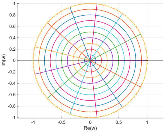
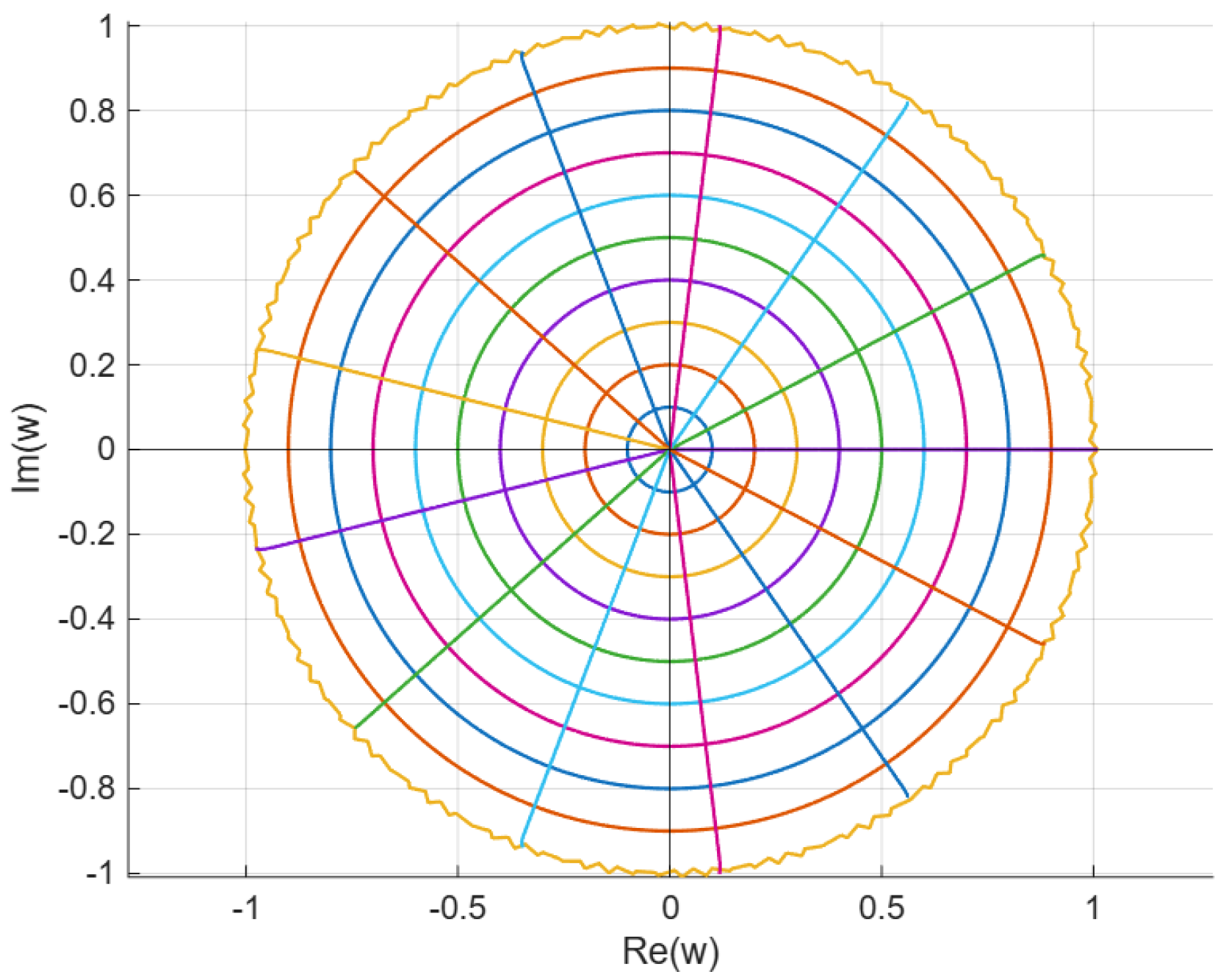
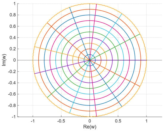
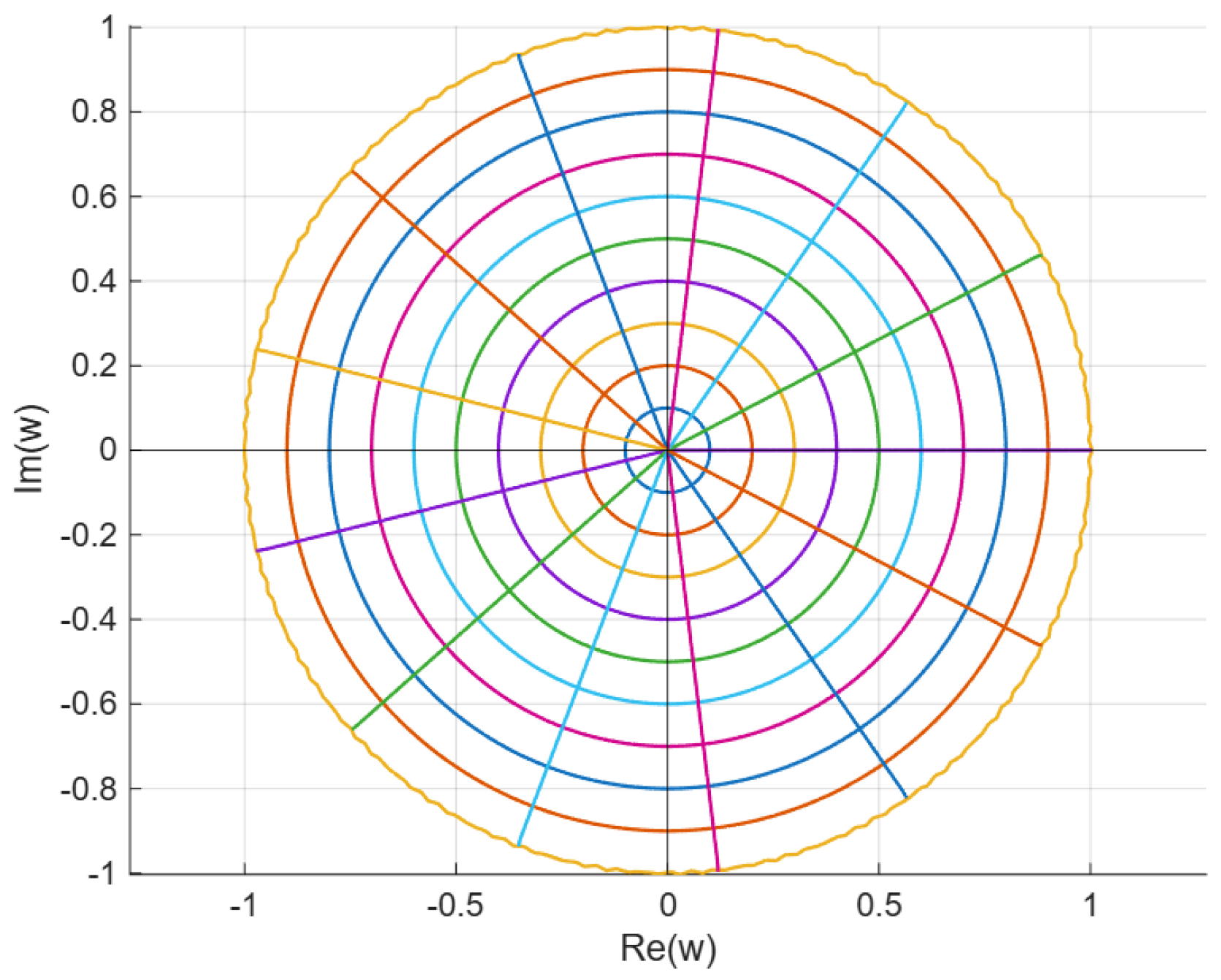
Visualization is used here as a complementary tool for interpreting the coefficient conditions obtained in the theoretical part. Rather than displaying the original unit disk separately, the following figures focus directly on the images of the disk under the $(\mathfrak{p},\mathfrak{q})$-Poisson distribution series, its negative-coefficient counterpart, and the associated operator. The same parameter values are kept whenever possible so that the geometric effects of the sign of the coefficients, the parameters $(\mathfrak{p},\mathfrak{q})$, the distribution parameter r, and the interpolation parameter $\mu$ can be compared clearly.

Image of the unit disk under the $(\mathfrak{p},\mathfrak{q})$-Poisson distribution series ${\mathcal{P}}_{\mathfrak{p},\mathfrak{q}}^r\left(z\right)$. The mapping is computed from the series definition

$${\mathcal{P}}_{\mathfrak{p},\mathfrak{q}}^r\left(z\right)=z+{\displaystyle \sum _{\ell =2}^{\infty }}{\displaystyle \frac{r^{\ell -1}{e}_{\mathfrak{p},\mathfrak{q}}^{-r}}{{[\ell -1]}_{\mathfrak{p},\mathfrak{q}}!}}{z}^{\ell },$$

which corresponds to Equation (6). The figure visualizes the geometric deformation induced by the $(\mathfrak{p},\mathfrak{q})$-Poisson distribution coefficients.

In Figure 1, the parameters are chosen as $\mathfrak{p}=0.95$, $\mathfrak{q}=0.85$, and $r=0.8$, satisfying $0<\mathfrak{q}<\mathfrak{p}<1$ and $r>0$. This choice represents a nontrivial $(\mathfrak{p},\mathfrak{q})$-regime close to the classical limit while still exhibiting a visible $(\mathfrak{p},\mathfrak{q})$-effect. The value of r is selected to ensure numerical stability of the series and to produce a clear geometric deformation of the unit disk under the mapping ${\mathcal{P}}_{\mathfrak{p},\mathfrak{q}}^r\left(z\right)$.

Figure 1. Image of the unit disk under the $(\mathfrak{p},\mathfrak{q})$-Poisson distribution series ${\mathcal{P}}_{\mathfrak{p},\mathfrak{q}}^r\left(z\right)$.

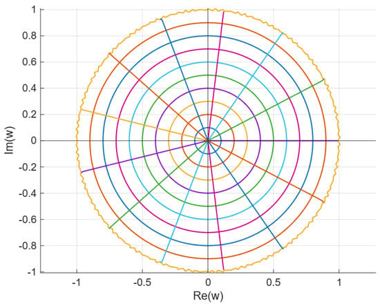
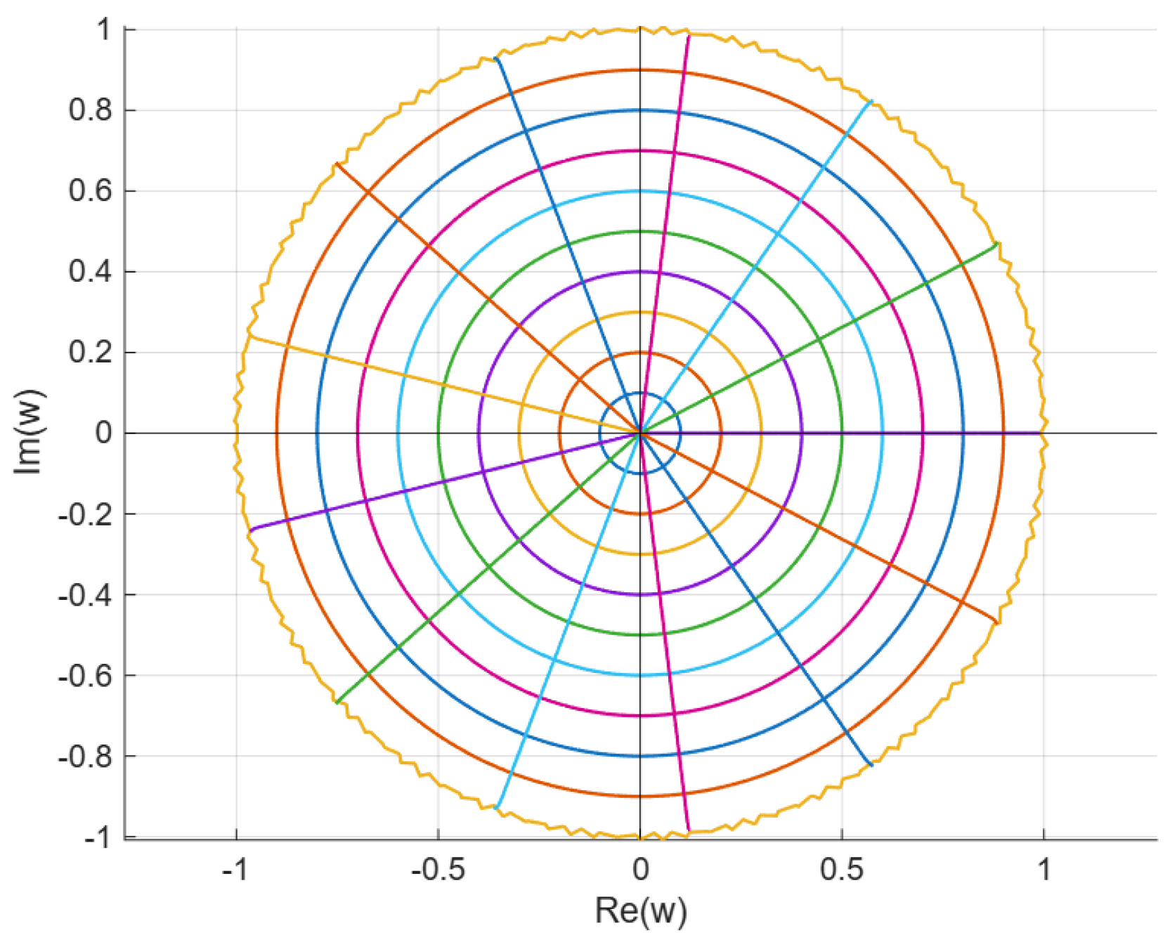
Image of the unit disk under the negative-coefficient $(\mathfrak{p},\mathfrak{q})$-Poisson distribution series $\mathcal{T}{\mathcal{P}}_{\mathfrak{p},\mathfrak{q}}^r\left(z\right)$. The mapping is defined by

$$\mathcal{T}{\mathcal{P}}_{\mathfrak{p},\mathfrak{q}}^r\left(z\right)=z-{\displaystyle \sum _{\ell =2}^{\infty }}{\displaystyle \frac{r^{\ell -1}{e}_{\mathfrak{p},\mathfrak{q}}^{-r}}{{[\ell -1]}_{\mathfrak{p},\mathfrak{q}}!}}{z}^{\ell },$$

which corresponds to Equation (7). The figure highlights the geometric effect of reversing the signs of the nontrivial coefficients compared to Figure 1.

In Figure 2, the same parameter values $\mathfrak{p}=0.95$, $\mathfrak{q}=0.85$, and $r=0.8$ as in Figure 1 are employed in order to isolate the effect of the negative coefficients. Keeping $(\mathfrak{p},\mathfrak{q},r)$ fixed allows for a direct geometric comparison between ${\mathcal{P}}_{\mathfrak{p},\mathfrak{q}}^r\left(z\right)$ and its negative-coefficient counterpart $\mathcal{T}{\mathcal{P}}_{\mathfrak{p},\mathfrak{q}}^r\left(z\right)$, thereby illustrating how the sign change in the coefficients influences the image of the unit disk.

Figure 2. Image of the unit disk under the negative-coefficient $(\mathfrak{p},\mathfrak{q})$-Poisson distribution series $\mathcal{T}{\mathcal{P}}_{\mathfrak{p},\mathfrak{q}}^r\left(z\right)$.

Image of the unit disk under the operator $N_{\mathfrak{p},\mathfrak{q}}^{r,\mu }\left(z\right)$ defined by

$$N_{\mathfrak{p},\mathfrak{q}}^{r,\mu }\left(z\right)=(1-\mu ){\mathcal{P}}_{\mathfrak{p},\mathfrak{q}}^r\left(z\right)+\mu z{D}_{\mathfrak{p},\mathfrak{q}}{\mathcal{P}}_{\mathfrak{p},\mathfrak{q}}^r\left(z\right),$$

where $D_{\mathfrak{p},\mathfrak{q}}$ denotes the $(\mathfrak{p},\mathfrak{q})$-derivative given in Equation (3) and ${\mathcal{P}}_{\mathfrak{p},\mathfrak{q}}^r\left(z\right)$ is the $(\mathfrak{p},\mathfrak{q})$-Poisson distribution series defined in Equation (6). The figure illustrates the geometric effect of the interpolation parameter $0\le \mu \le 1$. In Figure 3, the parameters $\mathfrak{p}=0.95$, $\mathfrak{q}=0.85$, and $r=0.8$ are chosen as in Figure 1 and Figure 2 to maintain consistency, while the interpolation parameter $\mu =0.6$ is selected to demonstrate a nontrivial combination of ${\mathcal{P}}_{\mathfrak{p},\mathfrak{q}}^r\left(z\right)$ and $z{D}_{\mathfrak{p},\mathfrak{q}}{\mathcal{P}}_{\mathfrak{p},\mathfrak{q}}^r\left(z\right)$. This choice allows the geometric influence of the $(\mathfrak{p},\mathfrak{q})$-derivative term to be clearly observed without dominating the contribution of the original $(\mathfrak{p},\mathfrak{q})$-Poisson distribution series.

Figure 3. Image of the unit disk under the operator $N_{\mathfrak{p},\mathfrak{q}}^{r,\mu }\left(z\right)$.

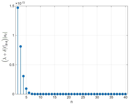
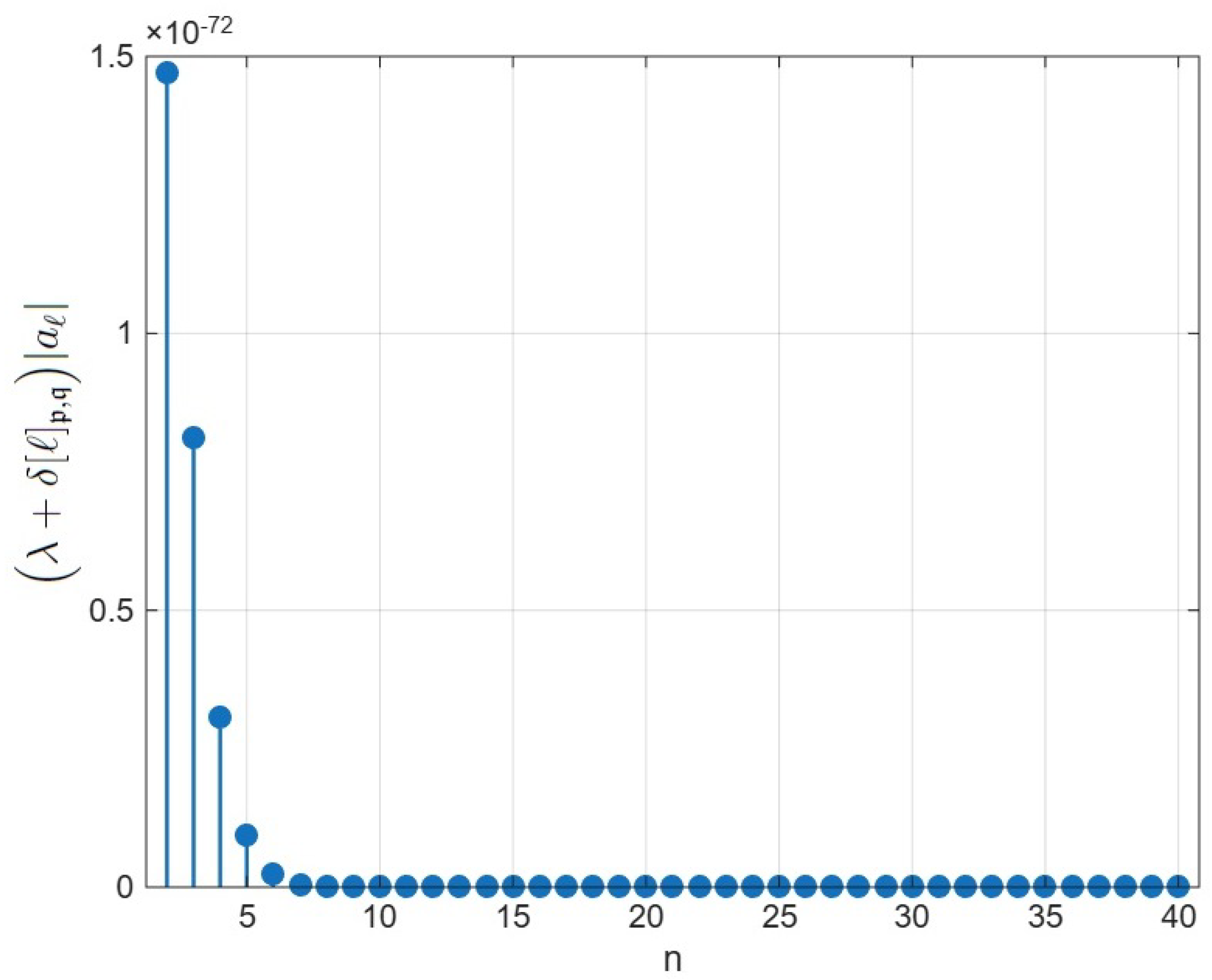
Regarding the decay behavior of the weighted coefficients associated with the $(\mathfrak{p},\mathfrak{q})$-Poisson distribution series ${\mathcal{P}}_{\mathfrak{p},\mathfrak{q}}^r\left(z\right)$, the plotted sequence is $(\lambda +\delta {[\ell ]}_{\mathfrak{p},\mathfrak{q}})\left|a_{\ell }\right|$, where $a_{\ell }={\displaystyle \frac{r^{\ell -1}{e}_{\mathfrak{p},\mathfrak{q}}^{-r}}{{[\ell -1]}_{\mathfrak{p},\mathfrak{q}}!}}$ denotes the Taylor coefficients of ${\mathcal{P}}_{\mathfrak{p},\mathfrak{q}}^r\left(z\right)$ given in Equation (6). This weighting corresponds to the coefficient conditions appearing in Theorems 1 and 2. Figure 4 provides a visual illustration of the coefficient condition in Theorems 1 and 2 by depicting the decay of the weighted coefficients $(\lambda +\delta {[\ell ]}_{\mathfrak{p},\mathfrak{q}})\left|a_{\ell }\right|$. Although the factor ${[\ell ]}_{\mathfrak{p},\mathfrak{q}}$ increases with ℓ, the rapid decrease in the coefficients $a_{\ell }$, induced by the $(\mathfrak{p},\mathfrak{q})$-factorial in the denominator, ensures that the weighted terms tend to zero. This behavior offers an intuitive justification for the convergence of the series ${\sum }_{\ell =2}^{\infty }(\lambda +\delta {[\ell ]}_{\mathfrak{p},\mathfrak{q}})\left|a_{\ell }\right|$ and supports the applicability of the coefficient criteria to the $(\mathfrak{p},\mathfrak{q})$-Poisson distribution series.

Figure 4. Decay behavior of the weighted coefficients associated with the $(\mathfrak{p},\mathfrak{q})$-Poisson distribution series ${\mathcal{P}}_{\mathfrak{p},\mathfrak{q}}^r\left(z\right)$.

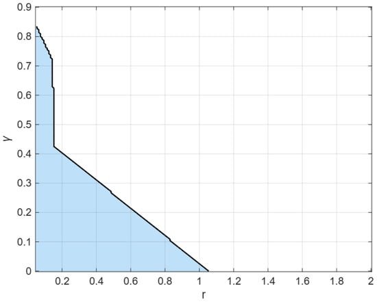
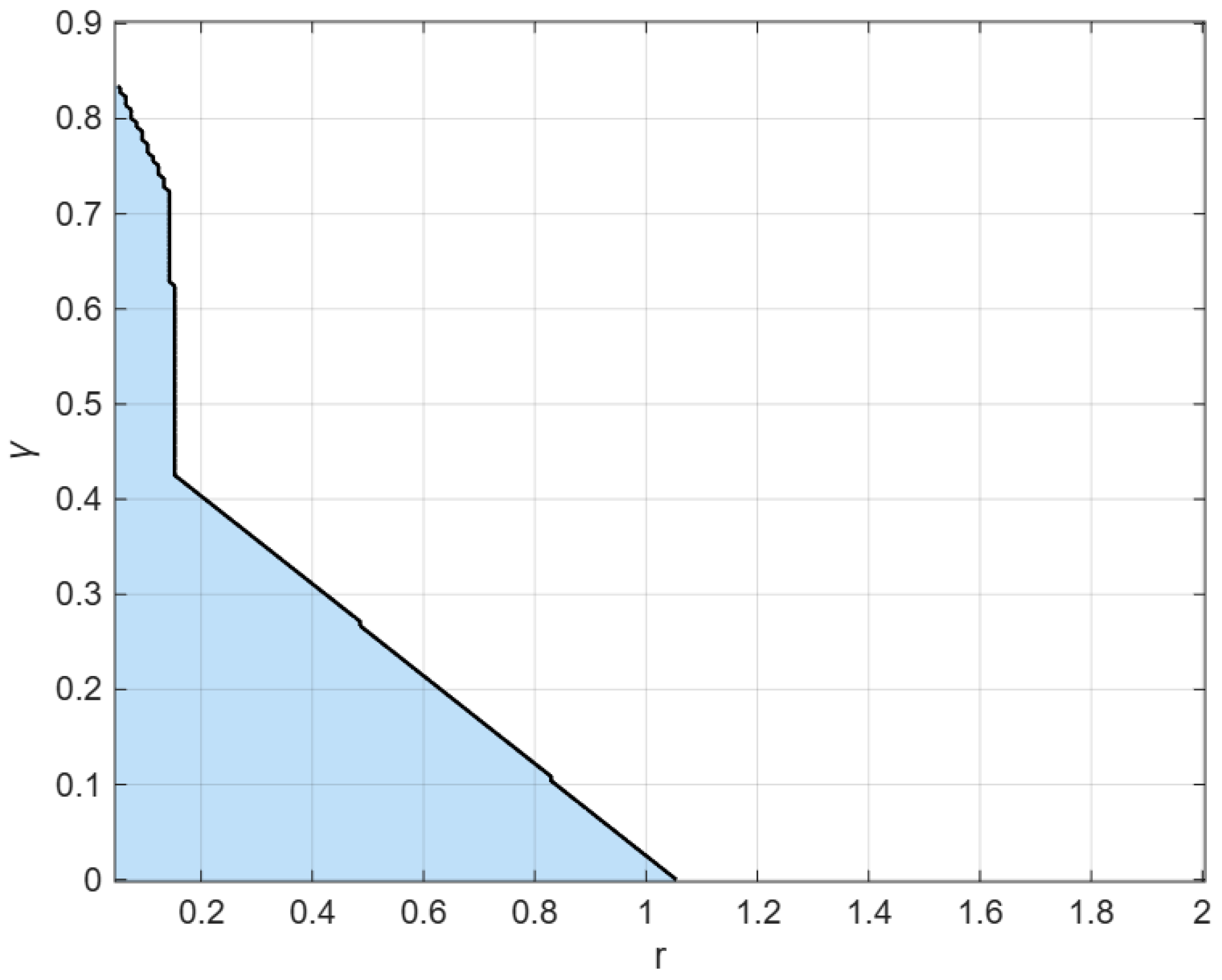
Figure 5 provides a geometric interpretation of the sufficient condition given in Theorem 3 by illustrating the admissible set of parameters $(r,\eta )$ in the $(r,\eta )$-plane. For fixed values of $\mathfrak{p}$, $\mathfrak{q}$, $\lambda$, and $\delta$, the shaded region represents all pairs $(r,\eta )$ for which inequality (13) is satisfied. Consequently, for every point in this region, the $(\mathfrak{p},\mathfrak{q})$-Poisson distribution series ${\mathcal{P}}_{\mathfrak{p},\mathfrak{q}}^r\left(z\right)$ is guaranteed to belong to the class $A_{\mathfrak{p},\mathfrak{q}}(\lambda ,\delta ,\eta )$.

Figure 5. Admissible region for Theorem 3 (Equation (13)).

The horizontal axis corresponds to the parameter $r>0$, which controls the size of the coefficients of the $(\mathfrak{p},\mathfrak{q})$-Poisson distribution series, while the vertical axis represents the threshold parameter $\eta$ appearing in the class definition. The figure clearly shows that, as parameter r increases, the admissible range of $\eta$ decreases. This behavior reflects the fact that larger values of r produce stronger geometric deformations, thereby imposing stricter requirements on the parameter $\eta$ for the class inclusion to hold.

The boundary curve separating the shaded and unshaded regions corresponds to the critical case where equality holds in (13). Points above this curve do not satisfy the sufficient condition of Theorem 3, although this does not necessarily imply that ${\mathcal{P}}_{\mathfrak{p},\mathfrak{q}}^r\left(z\right)$ fails to belong to the class; rather, it indicates that the theorem no longer guarantees the inclusion.

Overall, Figure 5 visualizes the interplay between the parameters r and $\eta$ and provides an intuitive understanding of how the coefficient growth, controlled by r, must be balanced by the class parameter $\eta$ to ensure membership of the $(\mathfrak{p},\mathfrak{q})$-Poisson distribution series in $A_{\mathfrak{p},\mathfrak{q}}(\lambda ,\delta ,\eta )$.

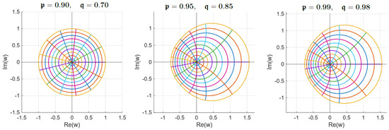
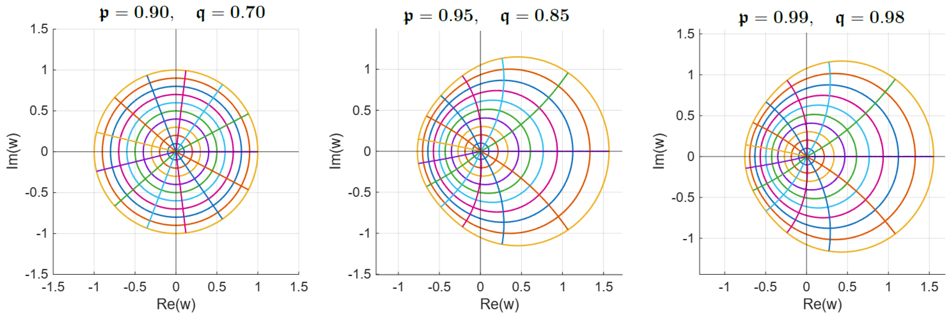
Figure 6 provides a visual comparison of the mapping ${\mathcal{P}}_{\mathfrak{p},\mathfrak{q}}^r\left(z\right)$ for several choices of $(\mathfrak{p},\mathfrak{q})$ with $0<\mathfrak{q}<\mathfrak{p}<1$, while keeping the parameter r fixed. As $(\mathfrak{p},\mathfrak{q})$ approaches $(1,1)$, the geometric behavior of the $(\mathfrak{p},\mathfrak{q})$-Poisson distribution series gradually resembles that of the classical Poisson-type mapping. This observation supports the limiting discussion and highlights the consistency of the $(\mathfrak{p},\mathfrak{q})$-generalization with the classical case.

Figure 6. Left to right: increasing values of $(\mathfrak{p},\mathfrak{q})$ approaching the classical limit.

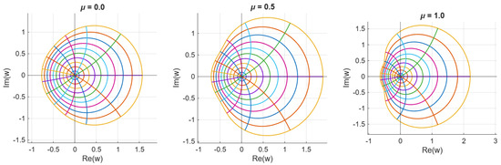
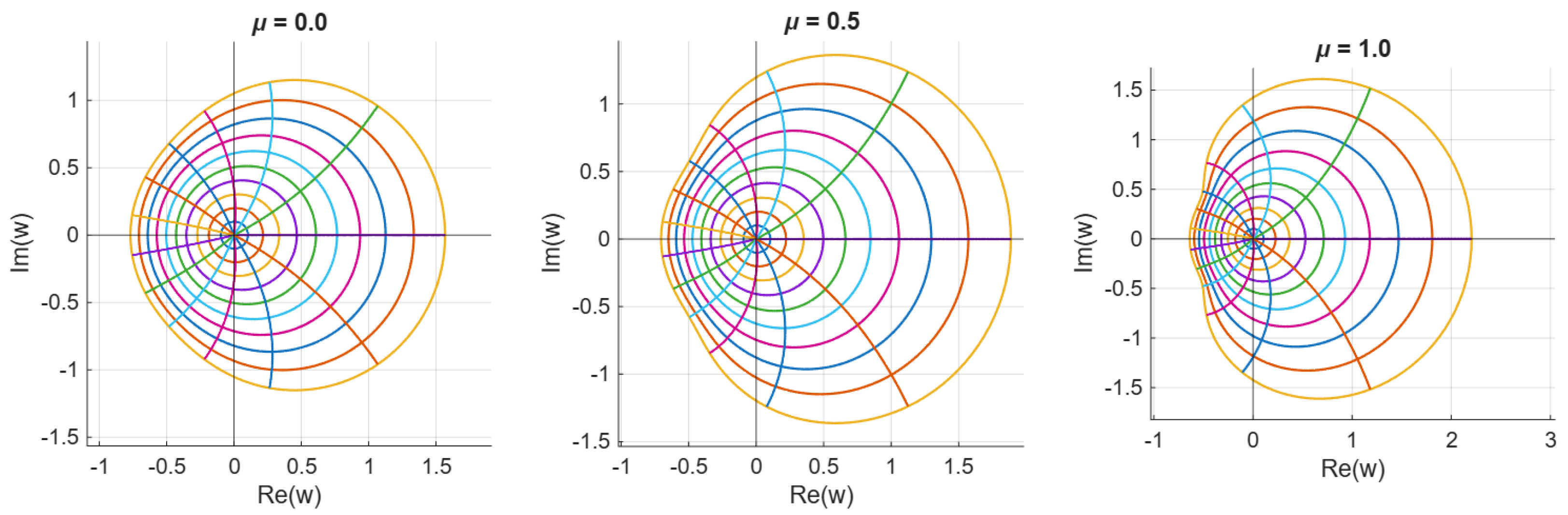
Effect of the parameter $\mu$ on the operator $N_{\mathfrak{p},\mathfrak{q}}^{r,\mu }\left(z\right)=(1-\mu ){\mathcal{P}}_{\mathfrak{p},\mathfrak{q}}^r\left(z\right)+\mu z{D}_{\mathfrak{p},\mathfrak{q}}{\mathcal{P}}_{\mathfrak{p},\mathfrak{q}}^r\left(z\right)$. The image of the unit disk is shown for $\mu =0$, $\mu =0.5$, and $\mu =1$, while $\mathfrak{p}$, $\mathfrak{q}$, and r are kept fixed. The figure illustrates how increasing $\mu$ enhances the influence of the $(\mathfrak{p},\mathfrak{q})$-derivative term in the operator.

Figure 7 illustrates the geometric effect of the interpolation parameter $\mu$ in the operator $N_{\mathfrak{p},\mathfrak{q}}^{r,\mu }\left(z\right)$. When $\mu =0$, the operator reduces to the $(\mathfrak{p},\mathfrak{q})$-Poisson distribution series ${\mathcal{P}}_{\mathfrak{p},\mathfrak{q}}^r\left(z\right)$, while $\mu =1$ corresponds to the pure derivative-based mapping $z{D}_{\mathfrak{p},\mathfrak{q}}{\mathcal{P}}_{\mathfrak{p},\mathfrak{q}}^r\left(z\right)$. Intermediate values of $\mu$ produce a smooth transition between these two cases, clearly demonstrating the role of $\mu$ in controlling the contribution of the $(\mathfrak{p},\mathfrak{q})$-derivative term.

Figure 7. Effect of parameter $\mu$ on the operator $N_{\mathfrak{p},\mathfrak{q}}^{r,\mu }\left(z\right)=(1-\mu ){\mathcal{P}}_{\mathfrak{p},\mathfrak{q}}^r\left(z\right)+\mu z{D}_{\mathfrak{p},\mathfrak{q}}{\mathcal{P}}_{\mathfrak{p},\mathfrak{q}}^r\left(z\right)$.

5. Conclusions

This paper introduced and investigated the class ${\mathcal{A}}_{\mathfrak{p},\mathfrak{q}}(\lambda ,\delta ,\eta )$ defined by the $(\mathfrak{p},\mathfrak{q})$-derivative. The main results consist of coefficient criteria for this class and for the negative-coefficient subclass $\mathcal{T}{\mathcal{A}}_{\mathfrak{p},\mathfrak{q}}(\lambda ,\delta ,\eta )$. In particular, a sufficient coefficient condition was obtained for the general analytic case, while a necessary and sufficient condition was derived for the corresponding subclass with negative coefficients.

These criteria were applied to the $(\mathfrak{p},\mathfrak{q})$-Poisson distribution series ${\mathcal{P}}_{\mathfrak{p},\mathfrak{q}}^r\left(z\right)$ and to the operator $N_{\mathfrak{p},\mathfrak{q}}^{r,\mu }\left(z\right)$. The results show how the parameters $\mathfrak{p}$, $\mathfrak{q}$, r, $\lambda$, $\delta$, $\eta$, and $\mu$ enter the coefficient inequalities governing class membership. Moreover, the limiting case $\mathfrak{p},\mathfrak{q}\to 1^{-}$ recovers the corresponding classical coefficient condition for $\mathcal{G}(\lambda ,\delta ,\eta )$, which confirms the consistency of the introduced two-parameter generalization.

The novelty of the study lies in combining the two-parameter $(\mathfrak{p},\mathfrak{q})$-derivative framework with Poisson-type distribution series, negative-coefficient analytic functions, and operator-based inclusion criteria. The graphical analysis further supports the theoretical findings by showing how the considered mappings deform the unit disk under comparable parameter choices. Possible extensions of the present work include the study of Fekete–Szegö-type inequalities and Bieberbach-type coefficient problems for the introduced class and its related operators.

Another possible direction is to use the present coefficient criteria as a basis for studying further convolution operators, radii problems, and geometric subclasses generated by other probability distributions or quantum-calculus operators. The graphical framework may also be developed for comparing parameter-dependent deformations in related classes of analytic and univalent functions.

References

- Wang, Z.G.; Gao, C.Y.; Yuan, S.M. On the univalency of certain analytic functions. J. Inequal. Pure Appl. Math. 2006, 7, 9. [Google Scholar]
- Ismail, M.E.H.; Merkes, E.; Styer, D. A generalization of starlike functions. Complex Var. Theory Appl. 1990, 14, 77–84. [Google Scholar] [CrossRef] [Scilit]
- Gasper, G.; Rahman, M. Basic Hypergeometric Series; Cambridge University Press: Cambridge, UK, 2004. [Google Scholar] [CrossRef] [Scilit]
- Chakrabarti, R.; Jagannathan, R. A (p, q)-oscillator realization of two-parameter quantum algebras. J. Phys. A 1991, 24, 711–718. [Google Scholar] [CrossRef] [Scilit]
- Kac, V.; Cheung, P. Quantum Calculus; Springer: New York, NY, USA, 2002. [Google Scholar] [CrossRef] [Scilit]
- Kamsrisuk, N.; Passary, D.; Ntouyas, S.K.; Tariboon, J. Quantum calculus with respect to another function. AIMS Math. 2024, 9, 10446–10461. [Google Scholar] [CrossRef] [Scilit]
- Khan, M.F.; AbaOud, M. New applications of fractional q-calculus operator for a new subclass of q-starlike functions related with the cardioid domain. Fractal Fract. 2024, 8, 71. [Google Scholar] [CrossRef] [Scilit]
- Altınkaya, Ş.; Yalçın, S. Poisson distribution series for certain subclasses of starlike functions with negative coefficients. Ann. Univ. Oradea Fasc. Math. 2017, 24, 5–8. [Google Scholar]
- Altınkaya, Ş.; Yalçın, S. Poisson distribution series for analytic univalent functions. Complex Anal. Oper. Theory 2018, 12, 1315–1319. [Google Scholar] [CrossRef] [Scilit]
- Porwal, S. An application of a Poisson distribution series on certain analytic functions. J. Complex Anal. 2014, 2014, 984135. [Google Scholar] [CrossRef] [Scilit]
- Yalçın, S.; Bayram, H. On harmonic univalent functions involving (p,q)-Poisson distribution series. Avrupa Bilim Teknol. Derg. 2021, 28, 1048–1051. [Google Scholar] [CrossRef] [Scilit]
- Akgül, A. Fekete–Szegö variations for some new classes of analytic functions explained over Poisson and Borel distribution series. Math. Methods Appl. Sci. 2025, 48, 9241–9252. [Google Scholar] [CrossRef] [Scilit]
- Silverman, H. Univalent functions with negative coefficients. Proc. Amer. Math. Soc. 1975, 51, 109–116. [Google Scholar] [CrossRef]
- Srivastava, H.M. Operators of basic (or q-) calculus and fractional q-calculus and their applications in geometric function theory of complex analysis. Iran. J. Sci. Technol. Trans. A Sci. 2020, 44, 327–344. [Google Scholar] [CrossRef] [Scilit]
- Santhiya, S.; Thilagavathi, K. Geometric properties of analytic functions defined by the (p,q) derivative operator involving the Poisson distribution. J. Math. 2023, 2023, 2097976. [Google Scholar] [CrossRef] [Scilit]
- Porwal, S.; Kumar, M. A unified study on starlike and convex functions associated with Poisson distribution series. Afr. Mat. 2016, 27, 1021–1027. [Google Scholar] [CrossRef] [Scilit]
- Sakar, F.M.; Canbulat, A. A study on harmonic univalent function with (p,q)-calculus and introducing (p,q)-Poisson distribution series. J. Math. Ext. 2023, 17, 1–18. [Google Scholar] [CrossRef]
Disclaimer/Publisher’s Note: The statements, opinions and data contained in all publications are solely those of the individual author(s) and contributor(s) and not of MDPI and/or the editor(s). MDPI and/or the editor(s) disclaim responsibility for any injury to people or property resulting from any ideas, methods, instructions or products referred to in the content. |
© 2026 by the authors. Licensee MDPI, Basel, Switzerland. This article is an open access article distributed under the terms and conditions of the Creative Commons Attribution (CC BY) license.