A Memtransistor-Memristor-Based Chaotic Circuit with Attractors Coexistence

Abstract

Memtransistors, as multi-terminal devices with gate-tunable memristive behavior, offer new opportunities for nonlinear circuit design beyond conventional two-terminal memristors. The paper proposes a novel four-dimensional chaotic oscillator by integrating a three-terminal memtransistor model with a memristor. The mathematical models of both devices are established, and their equivalent circuits are presented. Based on the memtransistor model, a chaotic circuit is constructed, and its dynamical behavior is investigated by the Lyapunov exponent spectrum, bifurcation diagram, dynamical map, and other tools. It is found that the chaotic circuit has complex nonlinear characteristics and that the phenomenon of attractor coexistence exists. Furthermore, the chaotic system is discretized by the Euler approach, and experiments on an STM32-based circuit confirm the reliability of the theoretical analysis. This work provides a hardware-validated platform for studying memtransistor-based nonlinear circuits and may find applications in chaos-based secure communication and neuromorphic computing.

1. Introduction

In 1971, Chua proposed the memristor concept and called it the fourth basic circuit element in addition to resistance, capacitance, and inductance [1]. In 2008, the Williams research team at Hewlett-Packard reported the physical realization of the memristor in Nature [2]. The implementation of the solid-state memristor attracted widespread attention from academia and industry, making the memristor a new research hotspot [3]. Previous studies have shown that memristors have significant application potential in areas such as logic circuits [4,5], neural networks [6,7], and nonlinear circuits [8,9]. For instance, Xiao et al. proposed an analog solver based on memristive crossbar arrays to accelerate LU decomposition for real-time color watermarking, achieving substantial improvements in latency and throughput [10]. Qian et al. designed a memristor-enhanced polynomial hyperchaotic map with high complexity and randomness and further developed a multi-channel image encryption algorithm with superior security and efficiency [11]. Yu et al. introduced a non-polynomial memristor model that decouples attractor scroll number from circuit resource consumption, enabling controllable multiscroll dynamics in Hopfield neural networks and FPGA-based image encryption [12].

As a nonlinear component, the voltage–current hysteresis of memristors depends on the frequency of the periodic excitation signal; therefore, it can be used for chaotic circuit design [13]. Firstly, Itoh and Chua implemented a memristive chaotic circuit by substituting Chua’s diode in the oscillator with a piecewise-linear memristor [8]. They established the equations of the memristive chaotic circuit, analyzed the circuit characteristics, and found that the equilibrium points of the memristive circuit are a set of line points, which distinguishes it from conventional chaotic circuits. After this, several researchers proposed various memristor-based chaotic circuits. A variety of special novel dynamical phenomena, such as attractor coexistence, coexisting bifurcation modes, and hidden attractors, have been discovered in memristor chaotic circuits [14,15,16,17].

An important application of memristor is artificial neural networks. The human brain can be composed of memristors [18]. Memristors can simulate synaptic and neuronal behaviors, thus constituting a novel neural network, where synapses are local passive memristors and neurons are composed of local active memristors [19]. Some evidence shows that neurons operate in a regime known as the chaotic edge, which may be essential for brain complexity, learning efficiency, adaptation, and so on [20,21]. Kumar, Strachan, and Williams proposed a network of chaotic elements to solve combinatorial or global optimization problems, which use chaos to generate pseudo-random signals to prevent global synchronization and find a global minimum during a constrained search [22]. Although two-terminal memristors can simulate the basic operations of neural networks, biological neural networks consist of thousands of synapses interconnected with each other and therefore require multi-terminal memristors. Therefore, Sangwan’s team at Northwestern University used molybdenum disulfide (MoS₂), which has a thickness of a single atomic layer, to develop a multi-terminal memtransistor [23]. The three-terminal memtransistor is a basic memtransistor structure made using silicon dioxide/silicon (SiO₂/Si) as the substrate. The monolayer MoS₂ film is generated by chemical vapor deposition on SiO₂/Si substrates, and thermal evaporation of metals is utilized to generate the drain and source electrodes in the MoS₂ strip, while the doped silicon layer serves as the gate electrode. 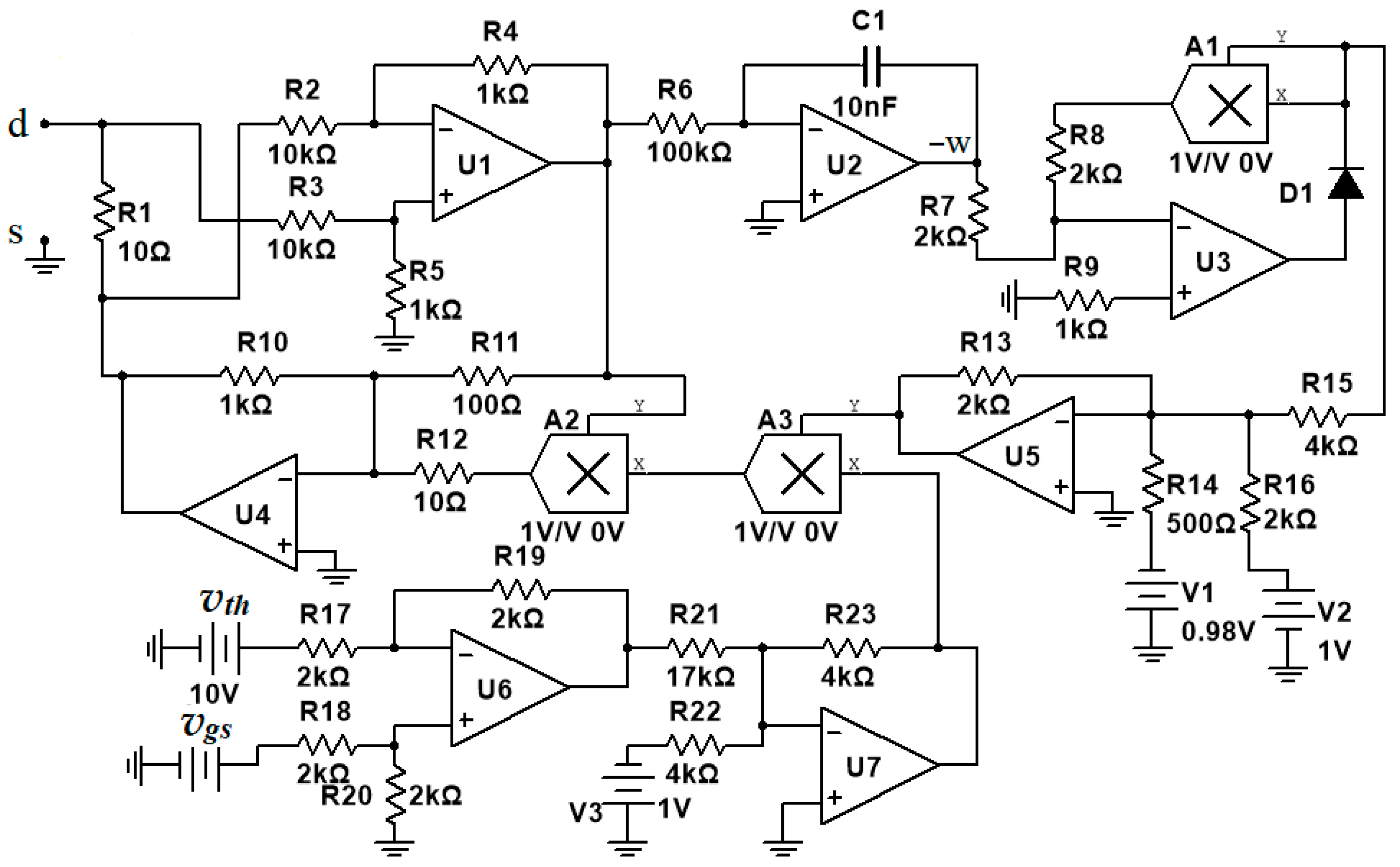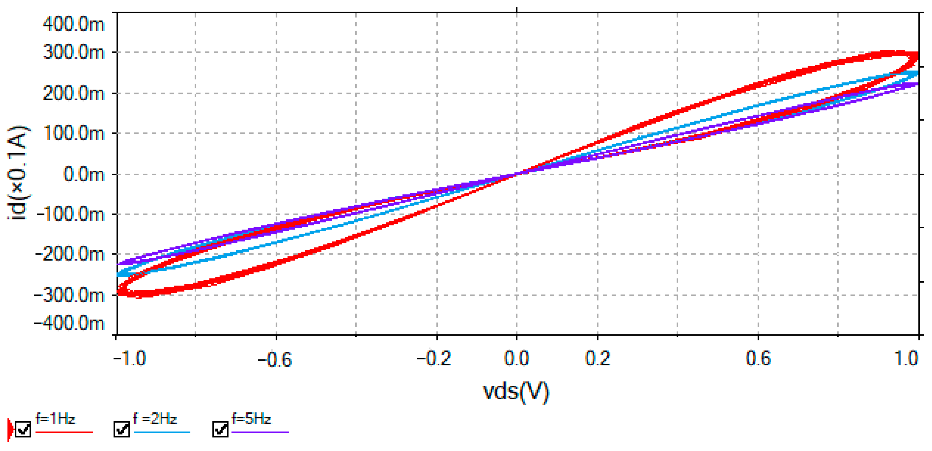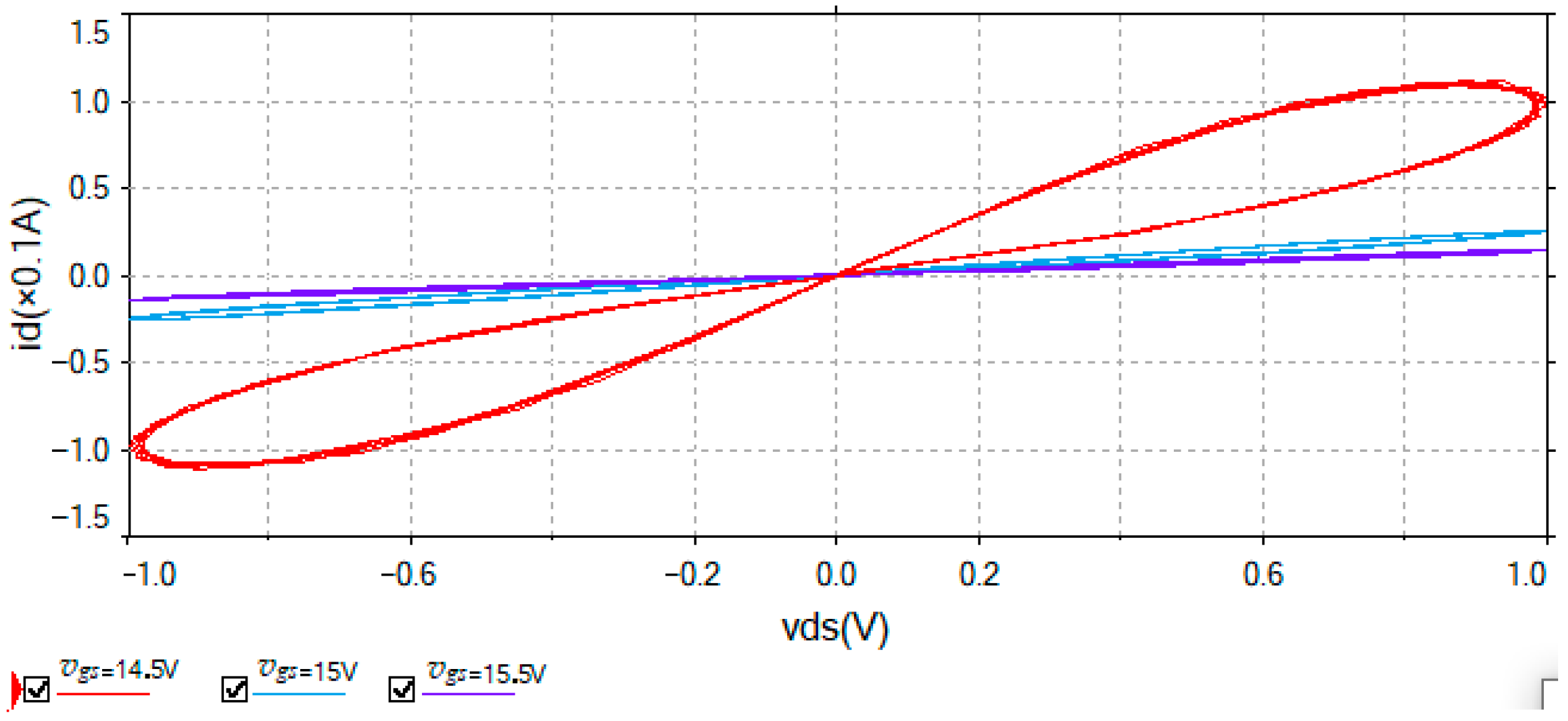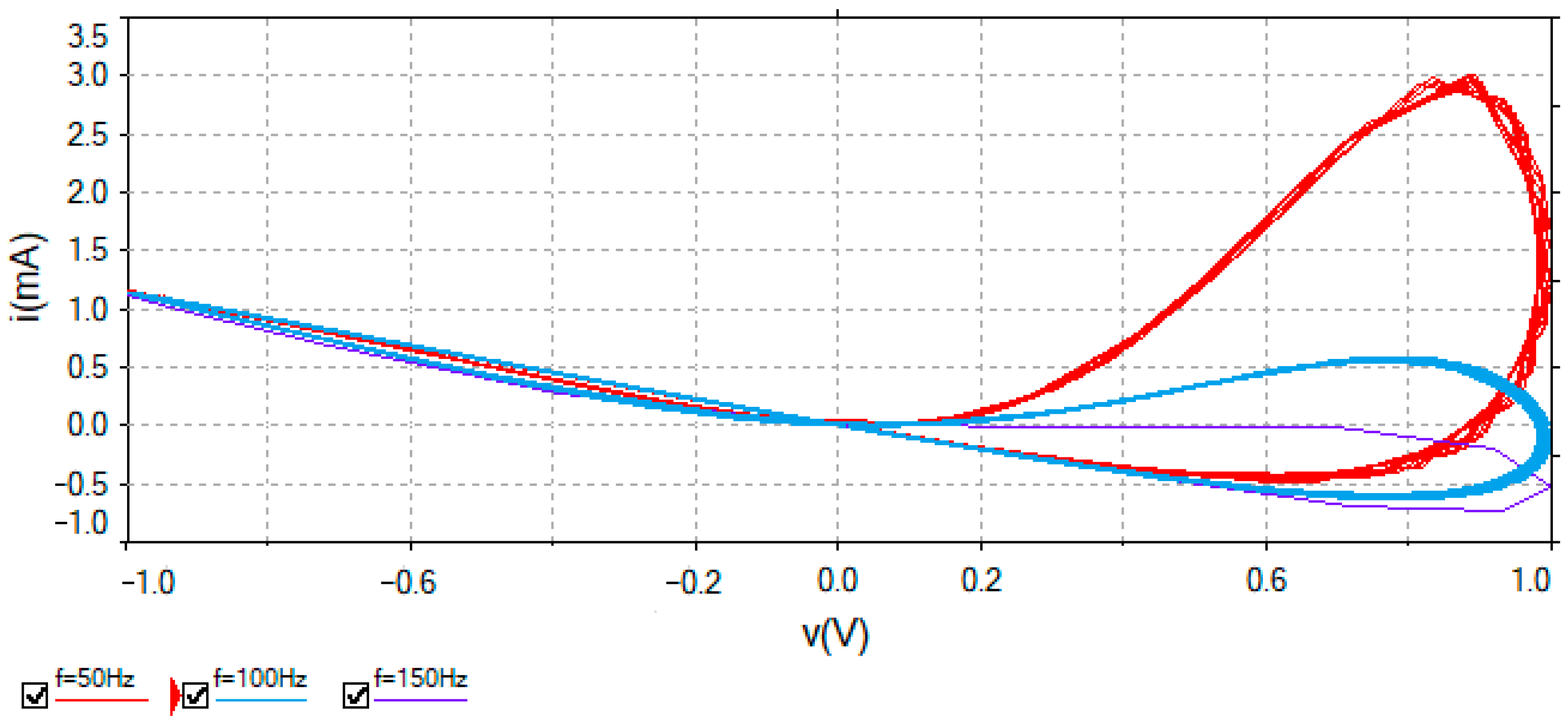Literature [23] uses a field-effect transistor with two memristors to represent a three-terminal memtransistor, which can not only realize the change in high and low resistances of memristors but also adjust the i_d-v_d curve through the gate voltage. Li and Liang published a short review in Nature for this purpose, pointing out that the memtransistors are expected to overcome the limitations of existing artificial intelligence (AI) systems and improve the artificial intelligence (AI) systems in terms of energy consumption and computational complexity [24]. As a result, memtransistors have attracted academic attention. Hao’s team realized a three-terminal memtransistor using gallium arsenide (GaSe) [25]. Wang, Liao, and Wong et al. constructed an MoS₂ three-terminal memtransistor with adjustable drain and gate using sapphire as the substrate [26]. A simple and expandable Li-well oxide memtransistor is presented in [27], a self-rectifying MoS₂ memtransistor with asymmetric metal contacts is described in [28], and Literature [29] describes scalable memtransistor arrays based on transition metal dichalcogenides. At present, research on memtransistors has just begun. To better develop the computational architecture of memtransistor-based neural networks, it is necessary to construct an appropriate circuit model for three-terminal memtransistors and explore their characteristics. Moreover, chaotic circuits based on three-terminal memtransistor should be designed and their dynamical characteristics analyzed to lay a foundation for memtransistor neural networks. Therefore, this paper proposes a memtransistor model, establishes an equivalent circuit, and analyses its characteristics. Based on this memtransistor model, a memtransistor chaotic circuit is constructed in combination with a memristor. The characteristics of the chaotic circuit are analyzed, and experimental verification is provided.

Despite these advances, several research gaps remain. First, most existing memristor-based chaotic circuits employ two-terminal memristors, which lack the gate-tunable controllability offered by three-terminal memtransistors. Second, while attractor coexistence has been reported in various memristive systems, systematic experimental validation on hardware platforms remains limited. Third, the combination of a memtransistor and a memristor in a single chaotic oscillator has rarely been explored, and the mechanisms governing multistability in such hybrid systems are not well understood.

To address these gaps, this work makes the following contributions: (1) we design a chaotic oscillator that integrates a three-terminal memtransistor with a memristor, exploiting the gate-tunable nonlinearity of the memtransistor; (2) we systematically analyze the coexistence of attractors using Lyapunov exponent spectra, bifurcation diagrams, and basins of attraction; and (3) we provide STM32-based experimental verification, including a discussion of DAC resolution and numerical precision effects.

The remainder of this paper is organized as follows. Section 2 introduces the memristor and memristor models and discusses their characteristics using emulator circuits. In Section 3, we build a memtransistor-based chaotic oscillator and analyze its dynamical behaviors. Circuit experiments are used to validate the theoretical analyses. Section 4 draws the conclusion.

2. Memtransistor and Memristor Models

Due to its nonlinear memory characteristics, the memtransistor can be utilized to design a chaotic oscillator. In order to better realize the chaotic oscillator, a memristor is also introduced. In the following, mathematical models of the memtransistor and memristor are proposed, and the equivalent circuits are built to analyze their characteristics.

2.1. A Memtransistor Model and Its Equivalent Circuit

Ref. [23] presents a memtransistor model, defining it as:

$$i_d=D\exp [{\displaystyle \frac{e(v_{gs}-v_{th})}{c_r{k}_{B}T}}][1-\exp (-{\displaystyle \frac{e{v}_{ds}}{k_{B}T}})]\exp [{\displaystyle \frac{{\mathrm{\Phi }}_b(w)}{k_{B}T}}],$$

(1)

$${\mathrm{\Phi }}_b(w)={\mathrm{\Phi }}_{b0}-{\displaystyle \frac{e}{{\epsilon }_s}}\sqrt{{\displaystyle \frac{w\Delta n}{4\pi }}}+\sqrt{{\displaystyle \frac{e}{4\pi {\epsilon }_s}}}{\left[{\displaystyle \frac{2en({\mathrm{\Phi }}_{b0}+A|v_{ds}|)}{{\epsilon }_s}}\right]}^{1/4},$$

(2)

$${\displaystyle \frac{dw}{dt}}=E{i}_d\{1-{[{(w-0.5)}^2+0.75]}^p\},$$

(3)

where i_d is the drain current, v_ds is the voltage between the drain and source terminals, v_gs is the voltage between the gate and source terminals, vth is the threshold voltage, Φ_b is the Schottky barrier height, w is the internal variable of the memtransistor, k_B is the Boltzmann’s constant, ε_s is the dielectric constant drain current, e is the charge of the electrons, n is the doping level, and the remaining variables are fitting parameters. Since Φ_b0 >> A|v_ds| in Ref. [23], Equation (2) is simplified as:

$${\mathrm{\Phi }}_b(w)={\mathrm{\Phi }}_{b0}-{\displaystyle \frac{e}{{\epsilon }_s}}\sqrt{{\displaystyle \frac{w\Delta n}{4\pi }}}+\sqrt{{\displaystyle \frac{e}{4\pi {\epsilon }_s}}}{\left[{\displaystyle \frac{2en{\mathrm{\Phi }}_{b0}}{{\epsilon }_s}}\right]}^{1/4}={k^{\prime }}_4-{k^{\prime }}_3\sqrt{w},$$

(4)

where ${k^{\prime }}_3={\displaystyle \frac{e}{{\epsilon }_s}}\sqrt{{\displaystyle \frac{\Delta n}{4\pi }}}$${k^{\prime }}_4={\mathrm{\Phi }}_{b0}+\sqrt{{\displaystyle \frac{e}{4\pi {\epsilon }_s}}}{\left[{\displaystyle \frac{2en{\mathrm{\Phi }}_{b0}}{{\epsilon }_s}}\right]}^{1/4}$.

If the voltage between the drain and source terminals v_ds is small enough, i.e., $\left|{\displaystyle \frac{e{v}_{ds}}{k_{B}T}}\right|<<1$, the Taylor expansion of $\exp (-{\displaystyle \frac{e{v}_{ds}}{k_{B}T}})$ is performed and is given as follows:

$$\exp (-{\displaystyle \frac{e{v}_{ds}}{k_{B}T}})=1-{\displaystyle \frac{e{v}_{ds}}{k_{B}T}}+{\displaystyle \frac{{\left(\frac{e{v}_{ds}}{k_{B}T}\right)}^2}{2!}}-{\displaystyle \frac{{\left(\frac{e{v}_{ds}}{k_{B}T}\right)}^3}{3!}}+\cdots \cdots .$$

(5)

If the first two terms of the Taylor expansion are taken, the relative error is $\left|R_1\right|\le 1.36({\displaystyle \frac{e{v}_{ds}}{k_{B}T}})$. When $\left|{\displaystyle \frac{e{v}_{ds}}{k_{B}T}}\right|=0.1$, the relative error is R₁ = 0.47%. By linearizing $\exp (-{\displaystyle \frac{e{v}_{ds}}{k_{B}T}})$ in Equation (2), i.e., taking the first two terms of the Taylor expansion, and substituting them into Equation (1), Equation (6) is obtained as:

$$v_{ds}={\displaystyle \frac{k_{B}T}{De}}\exp [{\displaystyle \frac{e(v_{th}-v_{gs})}{c_r{k}_{B}T}}]\exp [{\displaystyle \frac{{k^{\prime }}_3\sqrt{w}-{k^{\prime }}_4}{k_{B}T}}]i_d.$$

(6)

A window function is introduced to bound the internal state variable within a physically meaningful range and to model nonlinear dopant drift near the boundaries. If the internal variable w remains within a meaningful range, the window function can be removed to reduce the complexity of the theoretical analysis. Let $k_1={\displaystyle \frac{k_{B}T}{De}}$, $k_2={\displaystyle \frac{e}{c_r{k}_{B}T}}$, $k_3={\displaystyle \frac{{k^{\prime }}_3}{k_{B}T}}$, $k_4={\displaystyle \frac{{k^{\prime }}_4}{k_{B}T}}$ and $k_8=E$. By linearizing the natural exponential term in Equation (6) and removing the window function, the simplified mathematical model of the memtransistor can be written as:

$$\begin{array}{c}{v}_{ds}=k_1[1+k_2(v_{th}-v_{gs})](1+k_3\sqrt{w}-k_4)i_d,\\ {\displaystyle \frac{dw}{dt}}=k_8{i}_d.\end{array}$$

(7)

To further investigate the characteristics of this memtransistor, an equivalent circuit is shown in Figure 1 and is built using Multisim. The drain current i_d is converted into a voltage through resistor R₁. The signal operational amplifier U₁ and resistors R₂ to R₅ form a subtraction operation unit. Since the input of the subtraction operation unit is connected to the resistor R₁, it can extract the drain current signal. The operational amplifier U₂, resistor R₆ and capacitor C₁ form an integration operation unit, which integrates the output signal of operational amplifier U₁ to generate the state variable signal -w. The operational amplifier U₃, multiplier A₁, diode D₁ and resistors R₇ to R₉ form a square root operation unit, which performs square root operation on the state variable signal. The operational amplifier U₅, resistors R₁₃ to R₁₆ and voltage sources V₁ and V₂ form an addition operation unit, which performs DC biasing on the output of the square root operation unit. To achieve gate control, operational amplifier U₆, resistors R₁₇ to R₂₀ and voltage sources vth and v_gs form a subtraction operation unit, which calculates the difference between voltage v_gs and threshold voltage vth. The operational amplifier U₇, resistors R₂₁ to R₂₃ and voltage source V₃ form an addition operation unit, which adjusts the level of the output signal of operational amplifier U₆. Multiplier A₃ receives the output signals of operational amplifier U₅ and operational amplifier U₇ for multiplication operations. Multiplier A₂ receives the output signals of multiplier A₃ and operational amplifier U₁ for multiplication operations. The operational amplifier U₄ and resistors R₁₀ to R₁₂ form an addition circuit, which adds the output signal of multiplier A₂ to the output signal of operational amplifier U₁. Its output terminal is connected to resistor R₁ to generate the drain current i_d. If R₂ = R₃, R₄ = R₅, R₇ = R₈, R₉ = R₇//R₈, R₁₃ = R₁₆, R₁₇ = R₁₈ = R₁₉ = R₂₀ and R₂₂ = R₂₃ in the circuit, and the input ds is connected to the input voltage, it can be described as:

$$\begin{array}{l}{v}_{ds}={\displaystyle \frac{R_{10}}{R_{12}}}\cdot [1+{\displaystyle \frac{R_{23}}{R_{21}}}\cdot (v_{th}-v_{gs})](1+{\displaystyle \frac{R_{13}}{R_{15}}}\cdot \sqrt{w}-{\displaystyle \frac{R_{13}}{R_{16}}}\cdot V_1)i_d,\\ {\displaystyle \frac{dw}{dt}}={\displaystyle \frac{1}{R_6{C}_1}}\cdot {\displaystyle \frac{R_1{R}_4}{R_2}}{i}_d.\end{array}$$

(8)

Compared with (7), the parameters of the mathematical model are obtained as k₁ = R₁₀/R₁₂, k₂ = R₂₃/R21, k₃ = R₁₃/R₁₅, k₄ = R₁₃/R₁₆ and k₈ = R₁R₄/(R₂R₆C₁). k₁ represents the gain of the addition circuit, k₂ is linked to the difference between vth and v_gs, k₃ is releated to the square root operation, k₄ controls the DC bias, and k₈ determines the integration time constant. The meaningful range of w(0) is from 0.01 to 1.

When the resistance and capacitance values of the circuit are chosen as shown in Figure 1 and a sinusoidal excitation signal of v_pk = 1V is added to the input ds, the v-i characteristics shown in Figure 2 are achieved by varying the frequency of the sinusoidal voltage. The v-i characteristics are similar to the characteristics of a memristor, presenting pinched hysteresis loops. The pinched hysteresis loops pass through the origin, satisfying the memristor fingerprint. Moreover, the hysteresis loop area decreases as the excitation frequency increases. If the value of the voltage of v_gs is changed, the v-i characteristics shown in Figure 3 are acquired. The influence of the gate–source voltage v_g is similar to that of the excitation frequency, and the hysteresis lobe area also decreases as the voltage increases, which is in accordance with the characteristics of a memtransistor. Therefore, it can be observed that although the mathematical model was obtained when the voltage was sufficiently small, this mathematical model can still exhibit its memtransistor characteristics even when the voltage is not sufficiently low.

2.2. A Memristor Model and Its Equivalent Circuit

In order to realize the chaotic circuit, the following memristors are used:

$$\begin{array}{c}{i}_M=(c{z}^2-dz-e)v_M,\\ {\displaystyle \frac{dz}{dt}}=-k_{5}z-k_6{v}_M+k_{7}z{v}_M.\end{array}$$

(9)

where i_M is the current through the memristor, v_M is the voltage across the two terminals of the memristor, and z is the internal variable of the memristor.

To analyze the characteristics of the memristor, an equivalent circuit, as demonstrated in Figure 4, is established. When R₄ = R₈ in the circuit and the input terminal AB is connected to the input voltage, the following equation can be obtained from the equivalent circuit:

$$\begin{array}{c}{i}_M=[{\displaystyle \frac{R_3}{R_1{R}_2}}{z}^2-{\displaystyle \frac{R_3}{R_1{R}_{10}}}z-{\displaystyle \frac{1}{R_1}}({\displaystyle \frac{R_3}{R_9}}-1)]v_M,\\ {\displaystyle \frac{dz}{dt}}=-{\displaystyle \frac{1}{R_5{C}_1}}z-{\displaystyle \frac{1}{R_6{C}_1}}{v}_M+{\displaystyle \frac{1}{R_7{C}_1}}z{v}_M.\end{array}$$

(10)

Compared with (9), the parameters are obtained as c = R₃/(R₁R₂), d = R₃/(R₁R₁₀), e = (1/R₁)(R₃/R₉ − 1), k₅ = 1/(R₅C₁), k₆ = 1/(R₆C₁) and k₇ = 1/(R₇C₁).

If the resistor and capacitor values of the circuit are chosen as shown in Figure 4 and a sinusoidal signal with v_pk = 1V is added to the input AB, the v-i characteristics of the memristor demonstrated in Figure 5 are obtained. The v-i curves exhibit pinched hysteresis loops, and the hysteresis lobe area gradually decreases as the frequency increases, which accords with the memristive characteristics. The hysteresis loops are pinched at the origin, confirming the memristive nature of the device. The slight offset observed in some simulation traces is attributed to the transient response at the beginning of the simulation; after the initial transient decays, all loops precisely cross the origin. This behavior is consistent with the theoretical expectation for ideal memristors and does not indicate any flaw in the model.

3. Design of a Chaotic Circuit with a Memtransistor

3.1. A Memtransistor–Memristor-Based Chaotic Circuit

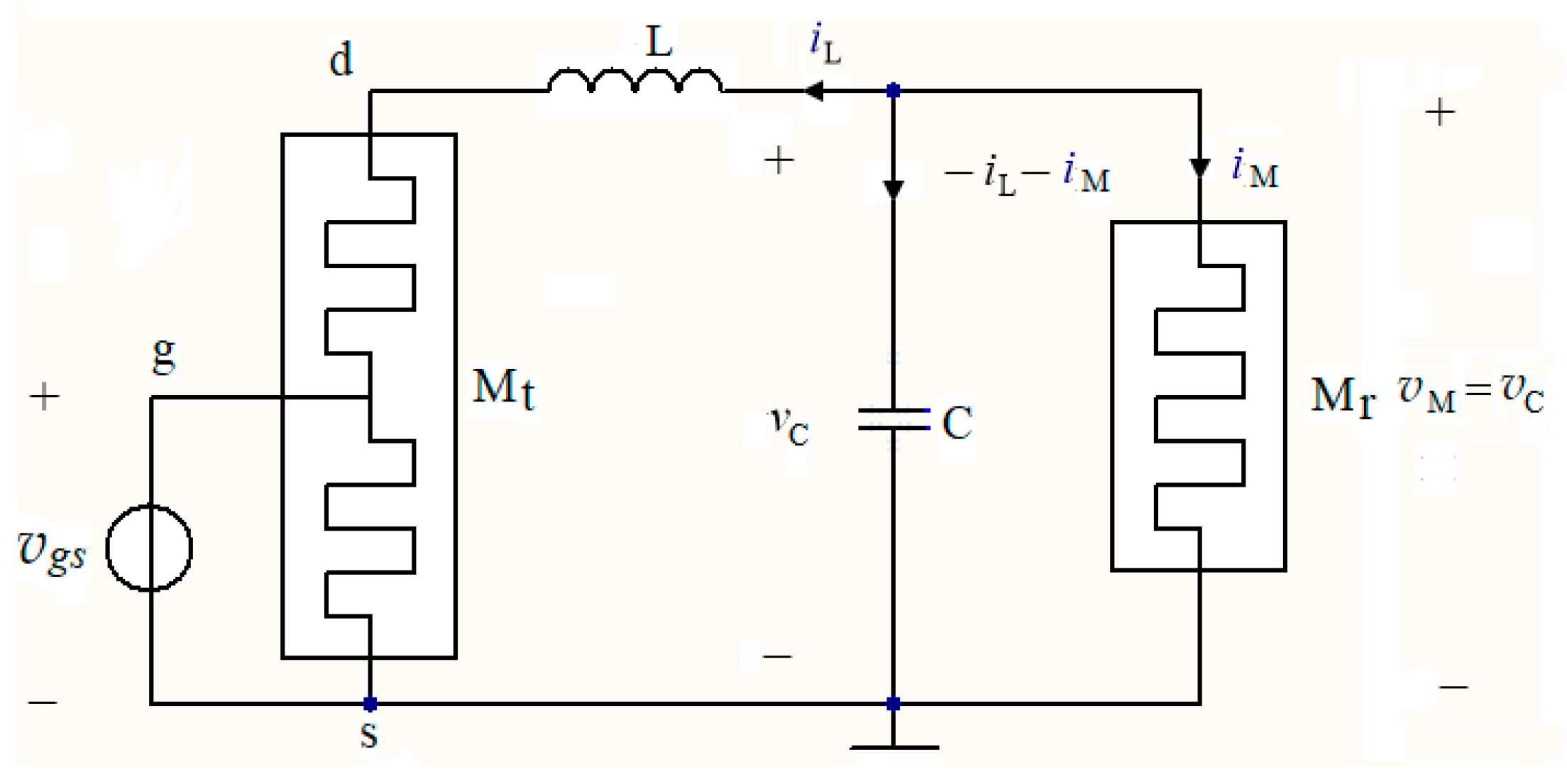
In the following section, the proposed memtransistor and memristor are used to construct the chaotic oscillator and analyze the nonlinear characteristics of the circuit.

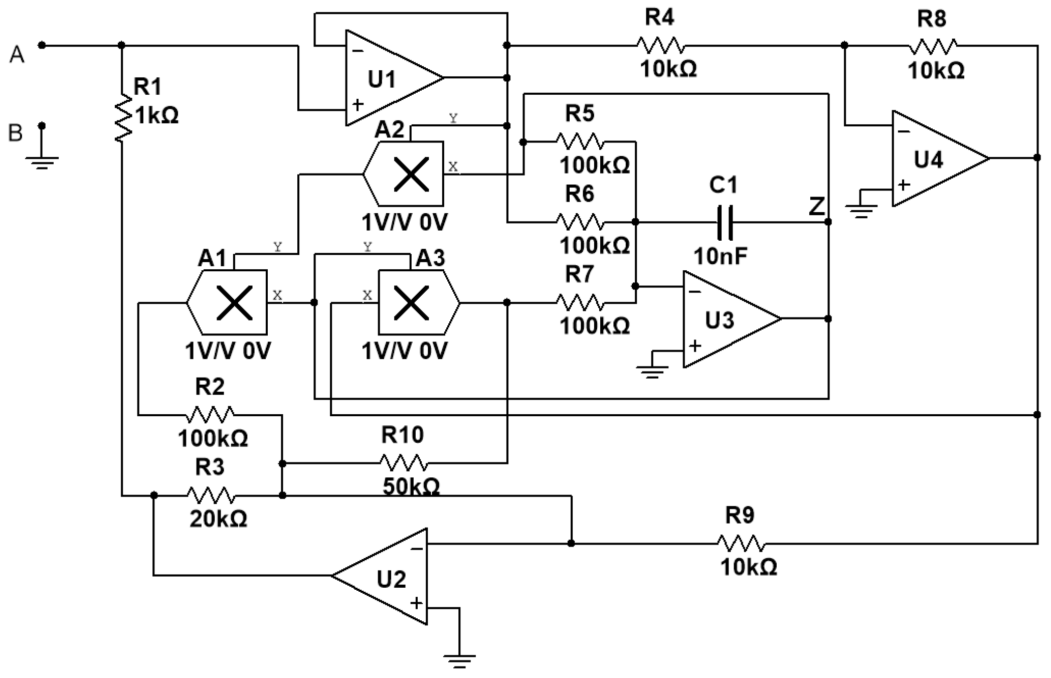
Based on the memtransistor and memristor models, a chaotic circuit is built, as demonstrated in Figure 6, which composes of a linear inductor, a linear capacitor, a memristor, a memtransistor, and a DC voltage source. According to Kirchhoff’s law and the component characteristics, if the inductor current i_L, capacitor voltage v_C, internal variable z of the memristor, and internal variable w of the memtransistor are selected as the state variables, the state equation of this circuit is written as:

$$\left\{\begin{array}{l}{\displaystyle \frac{d{i}_L}{dt}}={\displaystyle \frac{1}{L}}\{v_C-k_1[1+k_2(v_{th}-v_{gs})][1+(k_3\sqrt{w}-k_4)]i_L\},\hfill \\ {\displaystyle \frac{d{v}_C}{dt}}={\displaystyle \frac{1}{C}}[-i_L-(c{z}^2-dz-e)v_C],\hfill \\ {\displaystyle \frac{dz}{dt}}=-k_{5}z-k_6{v}_C+k_{7}z{v}_C,\hfill \\ {\displaystyle \frac{dw}{dt}}=k_8{i}_L,\hfill \end{array}\right.$$

(11)

where i_L is the current through the inductor; v_C is the voltage at two terminals of the capacitor; z is the internal variable of the memristor; w is the internal variable of the memtransistor; L is the inductance; C is the capacitance; vth is the threshold voltage of the memtransistor; v_gs is the gate–source bias voltage; c, d and e are the memristor model parameters; k₁, k₂, k₃, k₄, k₅, k₆, k₇ and k₈ are the memtransistor model parameters. The physical significance of Equation (11) lies in its description of energy exchange among the four storage elements. If we let x = i_L, y = v_C, a = 1/L and b = 1/C, Equation (11) can be transformed as

$$\left\{\begin{array}{l}\dot{x}=a\{y-k_1[1+k_2(v_{th}-v_{gs})](1+k_3\sqrt{w}-k_4)x\},\hfill \\ \dot{y}=b[-x-(c{z}^2-dz-e)y],\hfill \\ \dot{z}=-k_{5}z-k_{6}y+k_{7}yz,\hfill \\ \dot{w}=k_{8}x.\hfill \end{array}\right.$$

(12)

The physical significance of Equation (11) lies in its description of energy exchange among the four storage elements. If the parameters are set to a = 1, b = 0.33, c = 1.5, d = 0.1, e = 1.5, k₁ = 0.0001, k₂ = 50, k₃ = 0.9, k₄ = 0.01, k₅ = 1, k₆ = 0.6, k₇ = 1, k₈ = 0.00001, vth = 10, and v_gs = 3.8, with the initial conditions (0.2, 0.4, 0.78, 0.5), the Lyapunov exponents are obtained as LE₁ = 0.048, LE₂ = 0, LE₃ = −0.002 and LE₄ = −0.995, with a step size of 0.5 and a finish time of 10,000. The Lyapunov exponents are computed using the Jacobian method with Gram–Schmidt orthogonalization. The system state and the Jacobian matrix are evolved simultaneously using the fourth-order Runge–Kutta method. The Lyapunov dimension is D_L = 2.043, according to the Kaplan–Yorke formula. The largest Lyapunov exponent is LE₁ = 0.048 > 0, indicating exponential divergence of nearby trajectories—a hallmark of chaos. 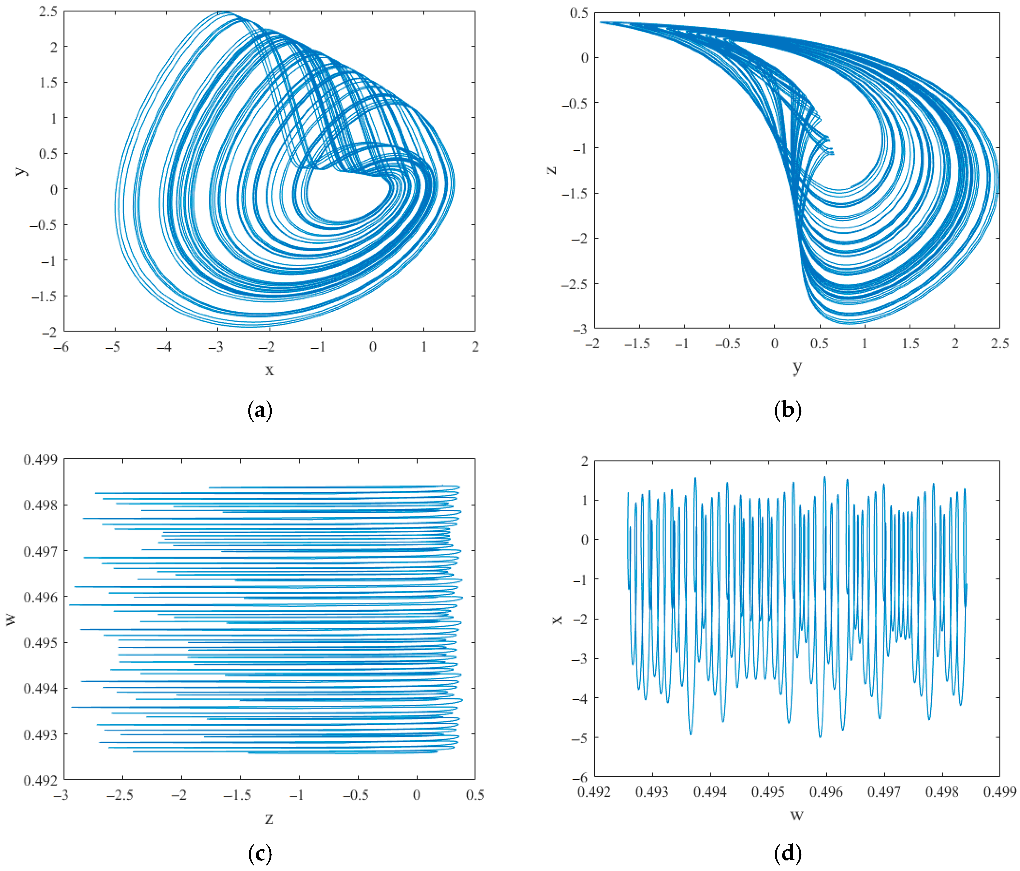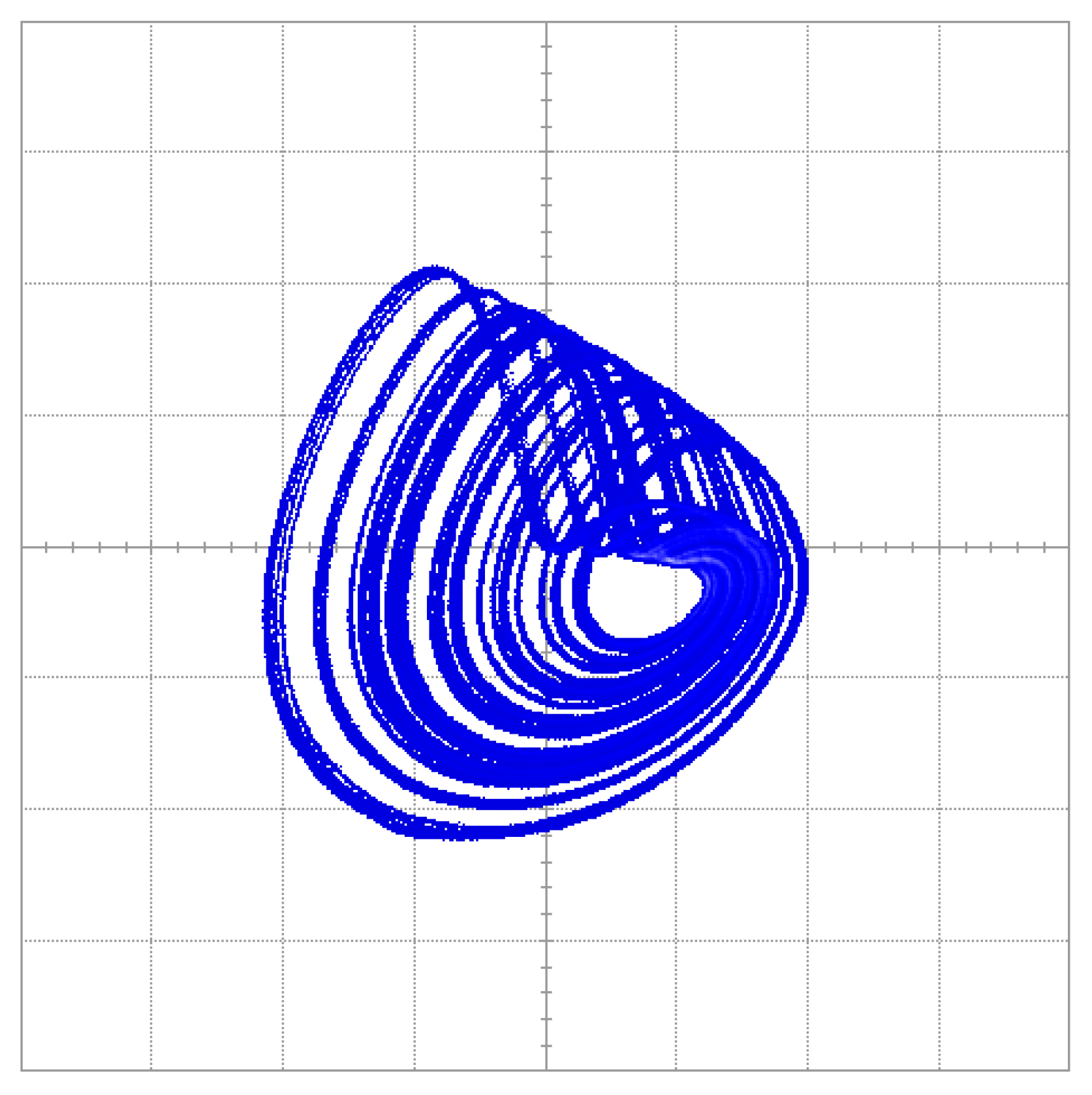The Lyapunov dimension D_L = 2.043 is fractional, confirming that the attractor is strange. Therefore, the system is in a chaotic state. 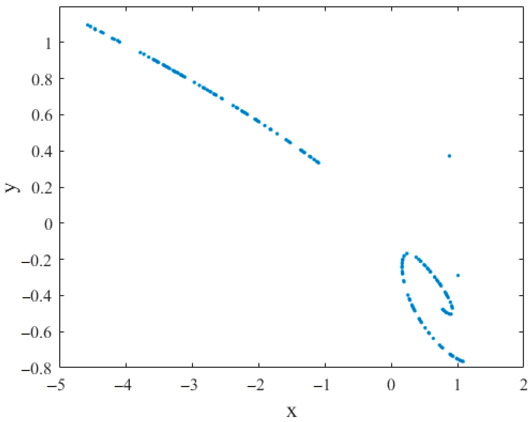In this case, the phase portraits of the system are presented in Figure 7, while the Poincaré map on z = 0 is plotted in Figure 8. Instead of a closed curve or a finite set of points, the map shows a dense, hierarchical structure. This is characteristic of a chaotic attractor, further confirming that the system exhibits chaotic dynamics.

3.2. Dissipation and Equilibrium Point Analysis of the System

The dissipation of Equation (12) can be written as:

$$\begin{array}{cc}\hfill \nabla \mathrm{V}& = {\displaystyle \frac{\partial \dot{x}}{\partial x}}+{\displaystyle \frac{\partial \dot{y}}{\partial y}}+{\displaystyle \frac{\partial \dot{z}}{\partial z}}+{\displaystyle \frac{\partial \dot{w}}{w}}=-a{k}_1[1+k_2(v_{th}-v_g)](1+k_3\sqrt{w}-k_4)\hfill \\ & -b(c{z}^2-dz-e)-k_5+k_{7}y.\hfill \end{array}$$

(13)

For Equation (13), there exists cases where ▽V < 0, which means that the equation is dissipative. Therefore, the attractor is likely to be chaotic.

If we set the left side of Equation (12) to zero, a line equilibrium of the system is obtained as E(0,0,0,w). Specifically, when the right-hand sides of Equation (12) are set to zero, the first three equations force x = 0, y = 0, and z = 0, regardless of w. The fourth equation then reduces to an identity that is satisfied for any w under the condition that the other variables are zero. This results in a continuum of equilibrium points (0,0,0,w) parameterized by w, forming a line in the 4D state space. Its Jacobi matrix is then as follows:

$$J=\left[\begin{array}{cccc}-a\{k_1[1+k_2(v_{th}-v_g)](1+k_3\sqrt{w}-k_4)\}& a& 0& 0\\ -b& be& 0& 0\\ 0& -k_6& -k_5& 0\\ k_8& 0& 0& 0\end{array}\right].$$

(14)

Substituting the parameters a = 1, b = 0.33, c = 1.5, d = 0.1, e = 1.5, k₁ = 0.0001, k₂ = 50, k₃ = 0.9, k₄ = 0.01, k₅ = 1, k₆ = 0.6, k₇ = 1, k₈ = 0.00001, vth = 10, v_gs = 3.8, as well as the initial condition (x(0), y(0), z(0), w(0)) = (0.2, 0.4, 0.78, 0.5), into Equation (14), the eigenvalues at the equilibrium are obtained as λ₁ = −1, λ₂ = 0 and λ_3,4 = 0.2222 ± 0.5056i. The negative real eigenvalue λ₁ = −1 corresponds to a stable direction, contracting trajectories along the corresponding eigenvector. The pair of complex conjugate eigenvalues with positive real parts, λ_3,4 = 0.2222 ± 0.5056i, corresponds to an unstable spiral, causing trajectories to oscillate with growing amplitude. This combination—stable along one direction and unstable in a spiral manner—defines an unstable saddle focus of index 2, which is precisely the type of equilibrium that can generate chaos through homoclinic orbits. When w(0) is within the range of 0.01 to 1, the eigenvalues of the system consist of one negative number, one zero, and one pair of conjugate complex numbers with positive real parts. Therefore, all the equilibrium points are saddle foci.

The stability analysis of the equilibrium points presented in this section serves not only a theoretical purpose but also provides the foundation for potential chaos control strategies. First, the stability of equilibrium points determines the system’s local dynamical behavior near these points. For a chaotic system, the presence of unstable saddle foci is a necessary condition for the existence of homoclinic or heteroclinic orbits, which can give rise to chaos. Second, understanding the stability of the line equilibrium is essential for controlling the chaotic system. In potential applications such as secure communication or neuromorphic computing, it may be desirable to suppress chaos or switch between different dynamical states. The stability analysis identifies the conditions under which the system is stable, providing guidelines for designing control laws.

3.3. Analysis of System Parameter Effects

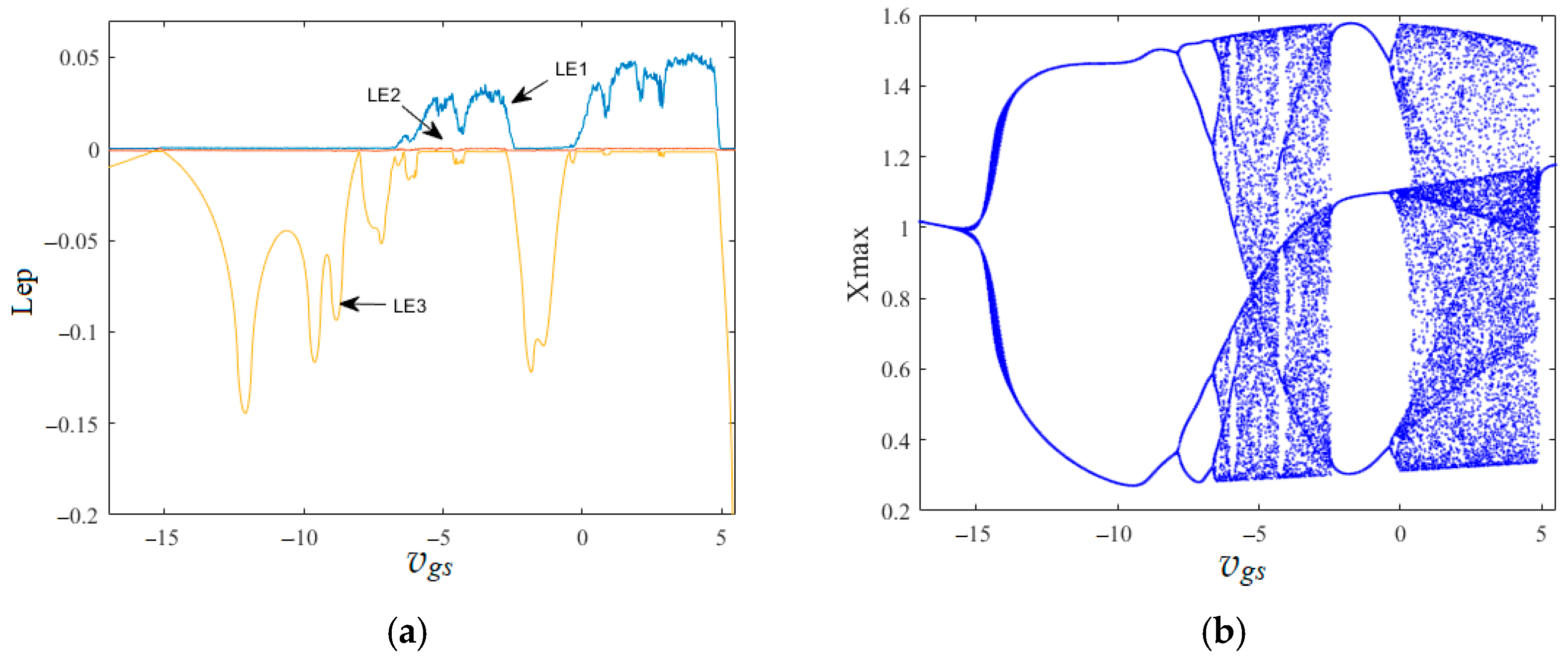
To explore the complex dynamical behavior of the memtransistor oscillator, the values of the easily controllable gate–source voltage v_gs and parameter b are used to analyze effects of system parameters. When the gate–source voltage v_gs is varied, the Lyapunov exponent spectrum and bifurcation diagrams of the oscillator are plotted in Figure 9a, where the smallest Lyapunov exponent is deleted for better observation (all Lyapunov exponent spectra are treated similarly below). The corresponding bifurcation diagrams (with a time interval of 0.01, a total duration of 1000, and 900 sampling points) are presented in Figure 9b. A system is classified as chaotic if the largest Lyapunov exponent LE₁ > 0, and as quasi-periodic or periodic if the largest Lyapunov exponent LE₁ = 0. In the bifurcation diagram, a dense set of points indicates chaos, whereas a finite set indicates periodic orbits. Therefore, the bifurcation diagram and Lyapunov exponent spectrum of the proposed oscillator are consistent with each other. 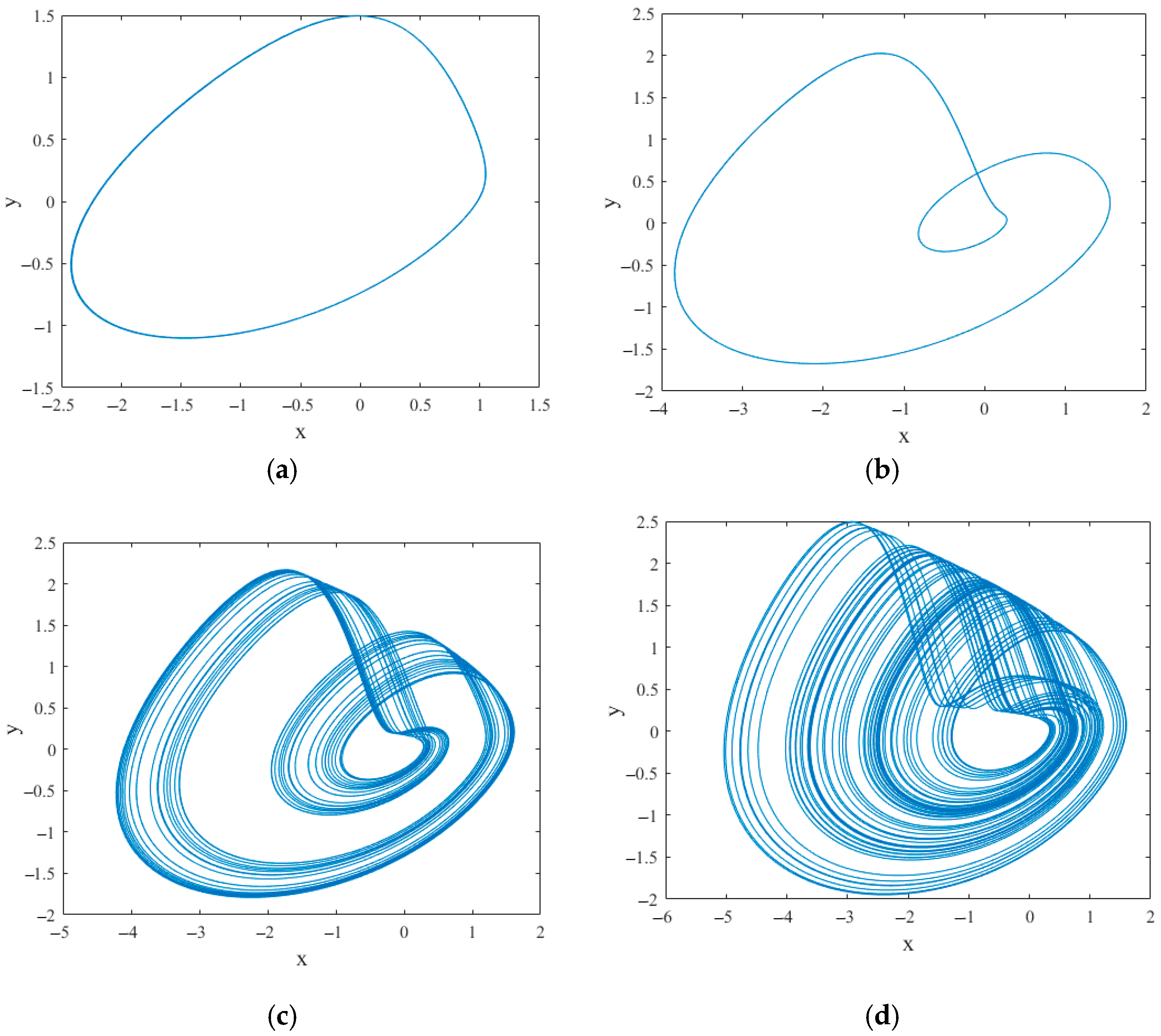The memtransistor oscillator enters the periodic bifurcation from a period-1 oscillation as the gate–source voltage v_gs increases and then enters a chaotic regime. Several periodic windows of different sizes appear after the system enters the chaotic regime. Specifically, when v_gs = −16, the system exhibits a period-1 oscillation, and its phase diagram is shown in Figure 10a. When v_gs = −9, the system exhibits a period-2 state, and its phase diagram is shown in Figure 10b. When v_gs = −5.8 and 4.0, the system is in a chaotic state, and the phase diagrams are shown in Figure 10c and Figure 10d, respectively.

The gate–source voltage v_gs varied from 17 V to 5.5 V in Figure 9 to capture the full range of dynamical transitions from periodic to chaotic behavior. This range is in line with the practica operating voltage requirements reported in the Literature [23] for the three-terminal memtransistors based on MoS₂. Sangwan et al. demonstrated gate-tunable behavior in MoS₂-based memtransistors with the gate–source voltage v_gs spanning approximately −40V to +40 V.

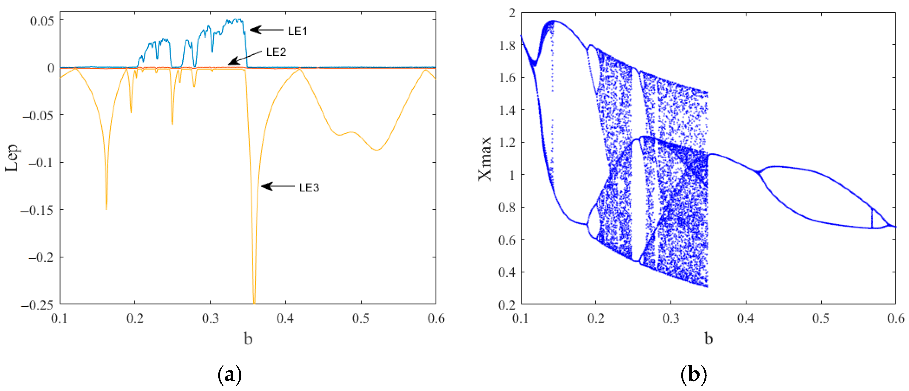
In addition to analyzing the effect of the gate–source voltage v_gs on the system, the effect of parameter b is also analyzed. Fixing the values of a = 1, c = 1.5, d = 0.1, e = 1.5, k₁ = 0.0001, k₂ = 50, k₃ = 0.9, k₄ = 0.01, k₅ = 1, k₆ = 0.6, k₇ = 1, k₈ = 0.00001, vth = 10 and v_gs = 3.8, and letting the value of b change from 0.1 to 0.6, with initial conditions of (0.2, 0.4, 0.78, 0.5), the Lyapunov exponent spectrum and the corresponding bifurcation diagram are obtained, as demonstrated in Figure 11. As shown in Figure 11, the system transitions between periodic, quasi-periodic, and chaotic regimes as parameter b varies, presenting complex dynamical behaviors.

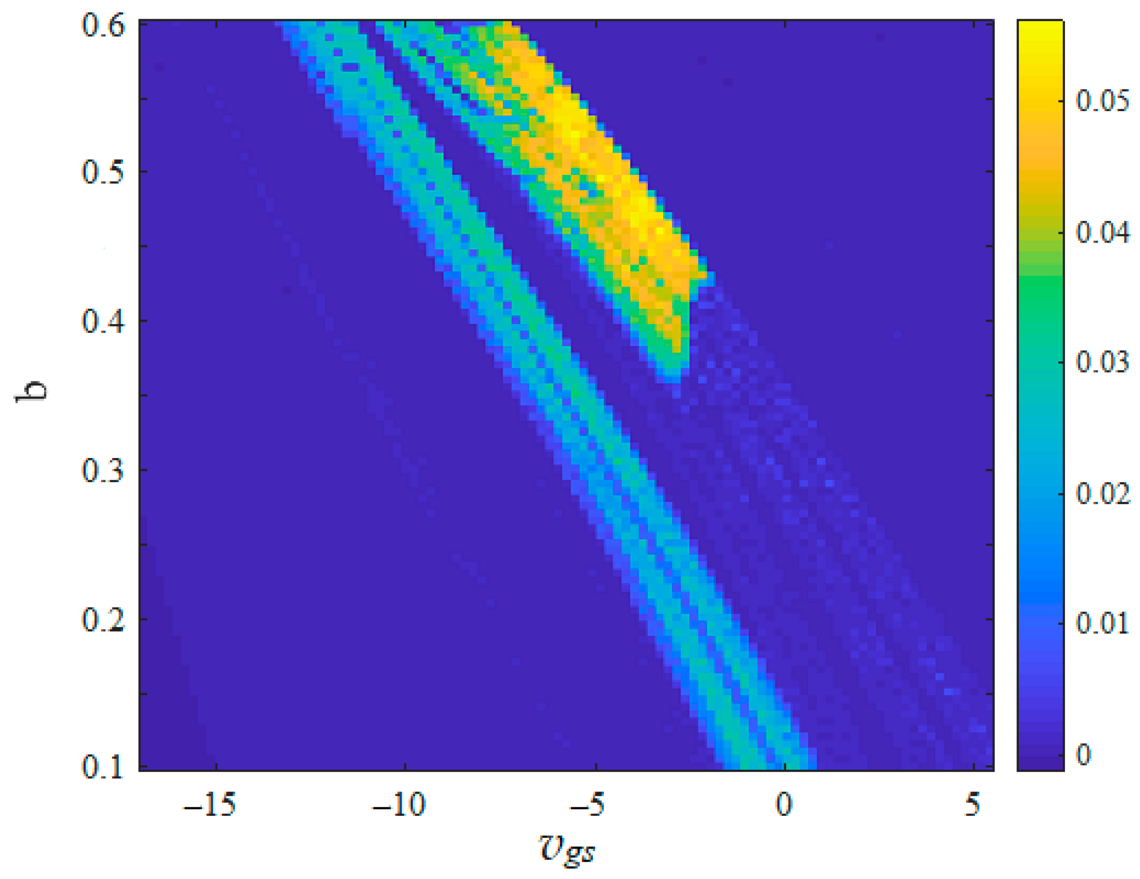
In order to study the simultaneous influence of the gate–source voltage v_gs and the inverse of the capacitance b, the dynamics map shown in Figure 12 is drawn, where the maximum Lyapunov exponent (MLE) is employed to describe the behaviors of the system. From Figure 12, it is clear that the system can demonstrate periodic, quasi-periodic and chaotic behaviors. The region of MLE > 0 is colored cyan-yellow to represent a chaotic state, while the region with MLE = 0 is colored blue to indicate periodic or quasi-periodic states.

3.4. Analysis of the Effect of Initial Values

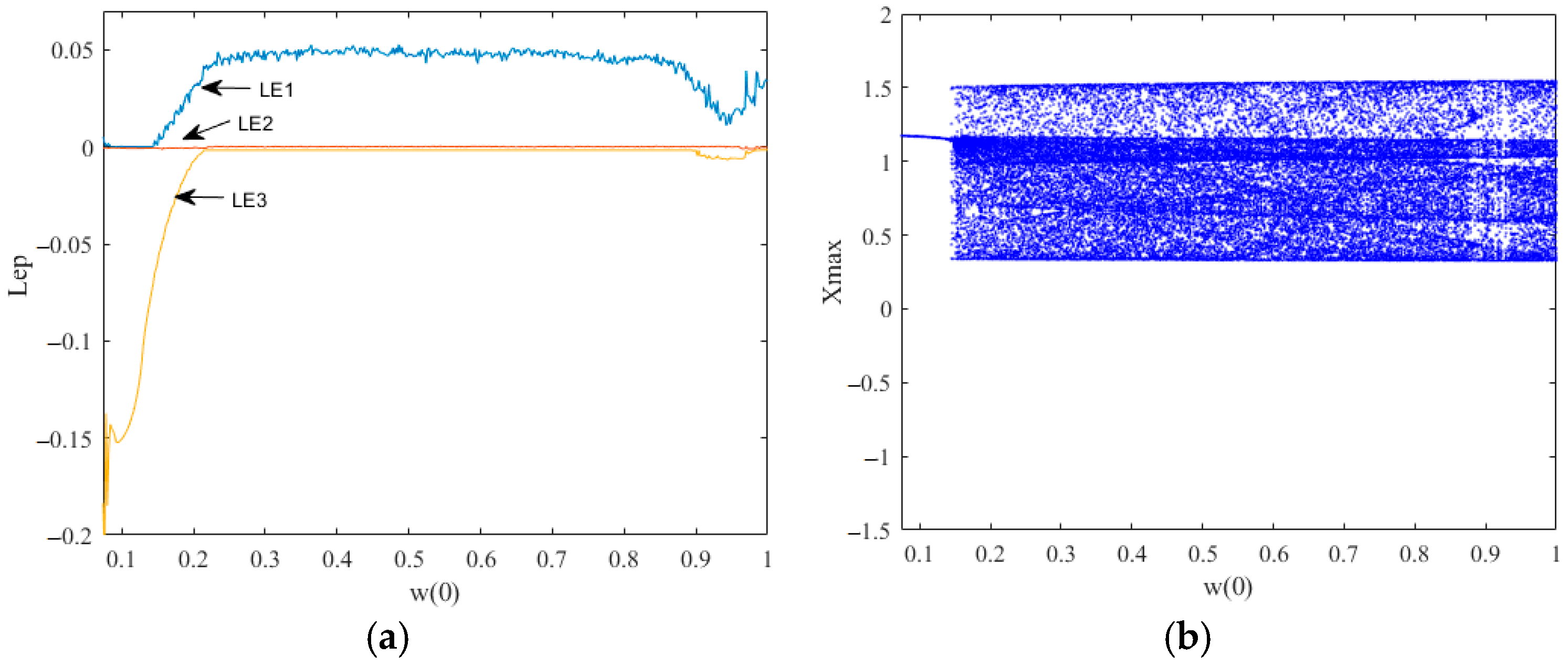
In chaotic systems, the dynamics depend not only on system parameters but also on initial conditions. With the parameters a = 1, b = 0.33, c = 1.5, d = 0.1, e = 1.5, k₁ = 0.0001, k₂ = 50, k₃ = 0.9, k₄ = 0.01, k₅ = 1, k₆ = 0.6, k₇ = 1, k₈ = 0.00001, vth = 10, v_gs = 3.8, together with the initial conditions of (x(0), y(0), z(0)) = (0.2,0.4,0.78), Figure 13 depicts the exponent spectrum and bifurcation diagram for the initial value w(0) ranging from 0.074 to 1. They coincide with each other. Although the system has both periodic and chaotic states, no periodic windows exist within the chaotic region. Since the system has a linear equilibrium point of O(0, 0, 0, w), the oscillator can possess the phenomenon of attractor coexistence. For a line equilibrium, the stability of the system depends critically on the specific value of w and, consequently, on the initial condition w(0). When the initial condition w(0) falls into different regions of this equilibrium line, the system may converge to distinct attractors since the local Jacobian eigenvalues vary along the line. This mechanism is fundamentally different from conventional chaotic systems with isolated equilibria, where attractor coexistence typically arises from multistability among separate fixed points. In the oscillator, the line equilibrium provides a continuum of possible stability profiles, and small perturbations in the initial condition w(0) can lead to qualitatively different asymptotic behaviors, including periodic, quasi-periodic, and chaotic attractors. The bifurcation diagram in Figure 13 with respect to w(0) explicitly demonstrates this sensitivity. As w(0) increases from 0.074 to 0.3, the system transitions from periodic to chaotic dynamics. 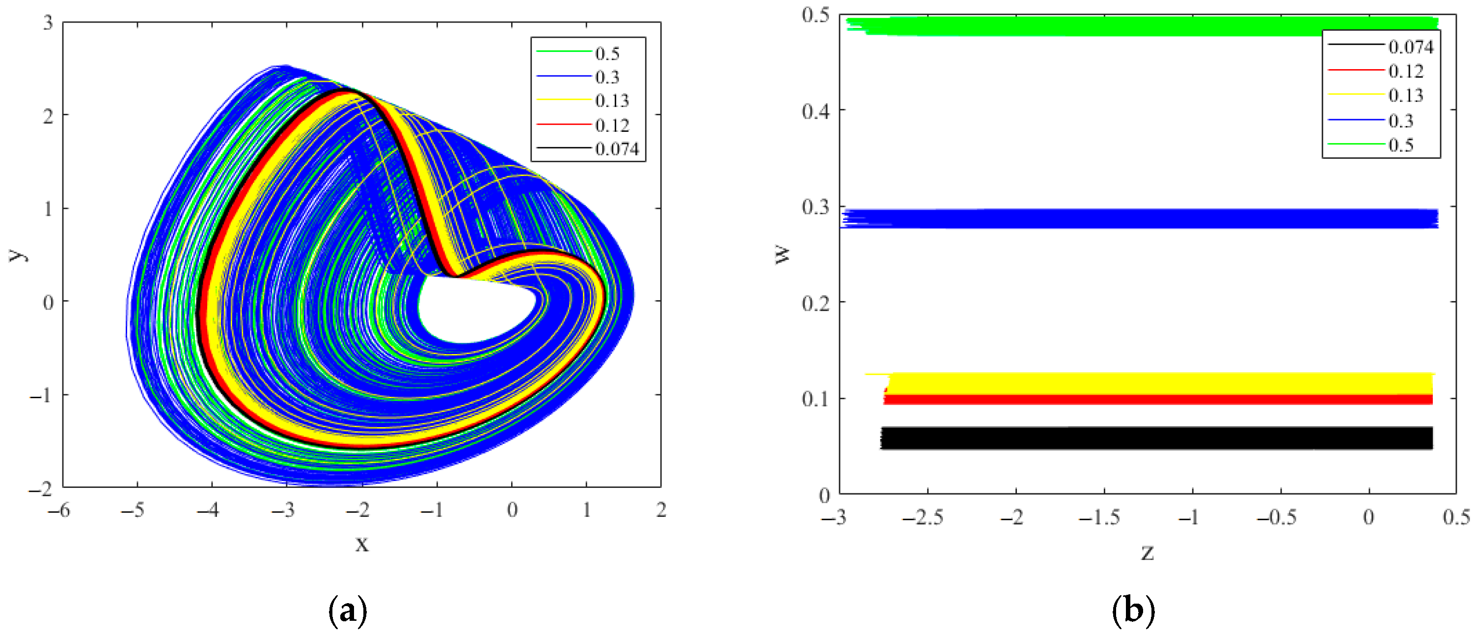To illustrate this phenomenon, the initial values w(0) = 0.074, 0.12, 0.13, 0.3, and 0.5 are considered to acquire the coexisting attractors shown in Figure 14. When w(0) is 0.074 and 0.12, the attractor is period-1; however, the attractor positions are not the same in the x–y and z–w planes. Hence, they are two coexisting periodic attractors. When w(0) = 0.13, the attractor is quasi-periodic. Under the circumstance of w(0) being 0.3 and 0.5, the coexisting attractors are chaotic. Unlike w(0), variations in x(0), y(0), and z(0) do not induce attractor coexistence under the same parameter set. This is because the line equilibrium is parameterized solely by w, whereas the other state variables vanish at equilibrium. Consequently, the system’s asymptotic behavior is uniquely determined by the initial value of w(0), while the other initial conditions only affect the transient trajectory without changing the final attractor type.

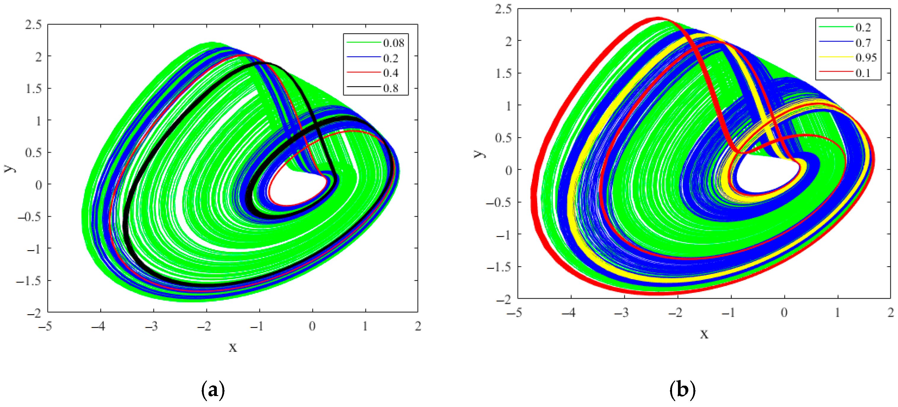
Moreover, different types of attractors coexist for certain parameter values. Taking the gate–source voltage v_gs of the memtransistor as an example, different types of attractor coexistence are presented in Figure 15, where the other parameters remain unchanged. As can be seen from Figure 15a, two period-2 attractors, one period-4 attractor, and one chaotic attractor coexist when v_gs = −10. Figure 15b demonstrates the coexistence of one period-2 attractor, one period-3 attractor and two different chaotic attractors when v_gs = −5.

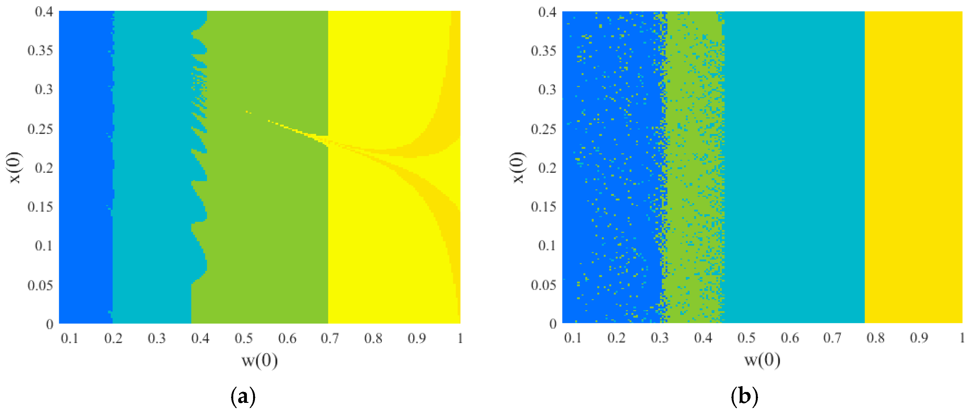
Coexisting attractors are a special phenomenon of nonlinear oscillators. They are sensitive to the initial values of the system and exist in certain chaotic systems [30,31,32]. To further illustrate the phenomenon of coexisting attractors, the basin of attraction is drawn in Figure 16. Figure 16 exhibits that the basin of attraction displays different regions corresponding to different attractors as the initial conditions x(0) and w(0) vary, implying the different types of attractors in the given value regions. In Figure 16a, there are five colors, implying the presence of five different types of attractors. However, Figure 16b has four colors, manifesting that there are four different types of attractors. Moreover, the color distribution in Figure 16b is different from that in Figure 16a, which indicates that the attractive basin alters with different values of the voltage v_gs. Each color corresponds to a distinct attractor type. For instance, the gemstone-blue color represents a chaotic attractor, while the yellow color signifies a period-2 attractor in Figure 16b. The color distribution shows that the system’s final state is highly sensitive to initial conditions, especially near the boundaries between colored regions.

It can be observed that the different types of coexisting attractors appear for different parameters and initial values. The coexistence of multiple attractors indicates that the oscillator is sensitive to both system parameters and initial conditions, which means that the system exhibits rich dynamical behaviors. Therefore, the system can be used for image encryption.

3.5. Circuit Design and Experimental Results

Analog and digital technologies are valuable methods for confirming the dynamical characteristics of nonlinear systems. Here, we adopt STM32 to implement the experimental research. First, utilizing the Euler approach, Equation (12) is discretized as Equation (15) to design a digital circuit. Equation (15) is expressed as

$$\left\{\begin{array}{l}x(n+1)=x(n)+a\{y(n)-k_1[1+k_2(v_{th}-v_{gs})](1+k_3\sqrt{w}-k_4)x(n)\}\Delta T,\hfill \\ y(n+1)=y(n)+b\{-x(n)-[c{z}^2(n)-dz(n)-e]y(n)\}\Delta T,\hfill \\ z(n+1)=z(n)+[-k_{5}z(n)-k_{6}y(n)+k_{7}y(n)z(n)]\Delta T,\hfill \\ w(n+1)=w(n)+k_{8}x(n)\Delta T,\hfill \end{array}\right.$$

(15)

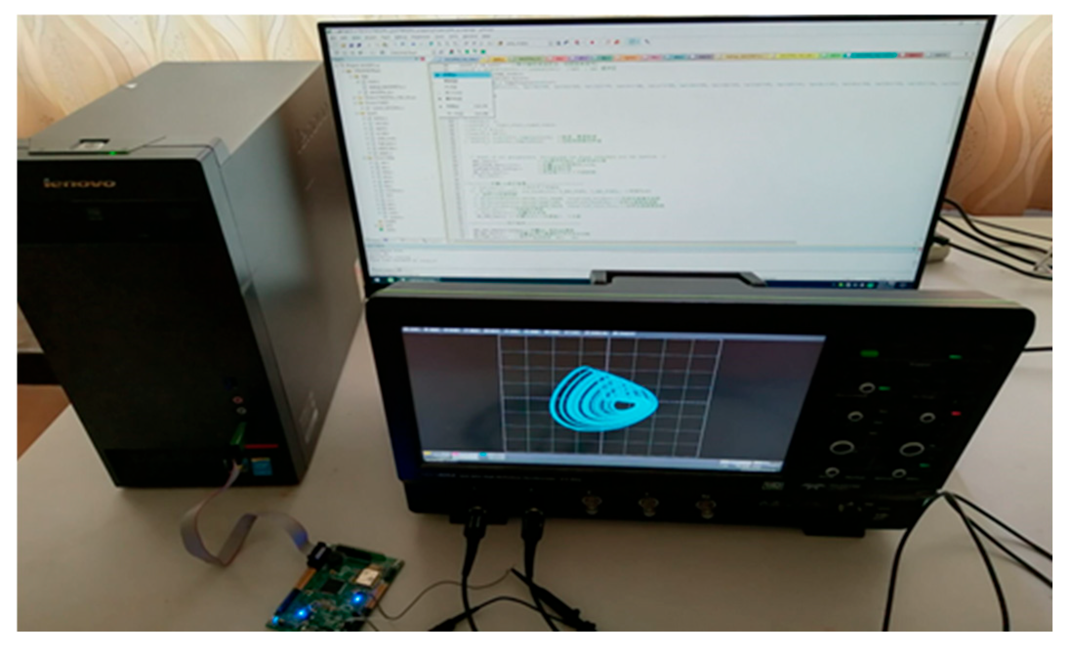
where ∆T is the step of discretization. In the STM32 implementation, the state variables w and z are directly mapped to 32-bit floating-point registers. The normalization range ensures that no additional scaling or offset compensation is required when converting between the mathematical model and the digital fixed-point or floating-point arithmetic. In order to satisfy the accuracy, we let ∆T = 0.0001. The experimental setup shown in Figure 17 is then applied to fulfil the circuit experiment. In this experimental setup, the STM32F407VET6 processor is the primary control chip. As a 32-bit microcomputer, its dominant frequency can reach up to 72 MHz. Moreover, it owns two 12-bit D/A converter modules, so it can output two separate analog signals simultaneously. Due to the use of a 12-bit DAC output, the resolution is 0.0244%. At an 8-bit resolution, the chaotic attractor degrades significantly, with trajectories appearing coarse and the fine fractal structure lost. At a 10-bit resolution, the attractor retains its overall shape but exhibits noticeable quantization artifacts, particularly in regions with high curvature. At a 12-bit resolution, the attractor morphology is visually indistinguishable from that of the ideal continuous case. The NMSE (Normalized Mean Squared Error) between the 12-bit quantized signal and the continuous simulation is 1.8 × 10⁻³, indicating that 12-bit resolution is sufficient for preserving chaotic dynamics. If the parameters are a = 1, b = 0.33, c = 1.5, d = 0.1, e = 1.5, k₁ = 0.0001, k₂ = 50, k₃ = 0.9, k₄ = 0.01, k₅ = 1, k₆ = 0.6, k₇ = 1, k₈ = 0.00001, vth = 10, and v_gs = 3.8, with the initial conditions (0.2, 0.4, 0.78, 0.5), the chaotic attractors can be seen on the oscilloscope, as shown in Figure 18, implying that the experimental results match well with the theoretical analysis. In the STM32 system, these parameters are stored as 32-bit floating-point numbers, which can represent values as small as 1.18 × 10⁻³⁸ with adequate precision. The key parameters used in the STM32 implementation, alongside their theoretical values, are summarized in

Table 1. Parameter comparison between the STM32 implementation and the theoretical model.

Parameter	Theoretical Value	STM32 Value	Relative Error
a	1	1.0000	0%
b	0.33	0.3300	0%
k1	0.0001	0.0001	0%
k8	0.00001	0.00001	0%
ΔT (step)	0.0001	0.0001	0%

. The relative errors between the experimental and numerical results are evaluated using NMSE for the attractor trajectories. For the chaotic attractor at w(0) = 0.5, the NMSE is 3.2 × 10⁻³, indicating good agreement between experiment and simulation. Therefore, this floating-point operation precision is sufficient for preserving attractor morphology. The Euler discretization step ∆T = 0.0001 ensures that the multiplication operations involving k₁ and k₈ do not suffer from underflow.

4. Conclusions

To explore the application of memtransistors in nonlinear circuits, the mathematical model as well as the emulator circuit of the memtransistori are proposed, and its fingerprint characteristics are illustrated. Based on the memtransistor model, a chaotic system is designed. In comparison to classical memristor-based oscillators that use two-terminal devices, the proposed chaotic circuit exploits a gate-tunable memtransistor, offering enhanced controllability. The complex dynamical behaviors of the oscillator are explored by some nonlinear tools, and it is found that the system is highly sensitive to both system parameters and initial conditions. The oscillator exhibits a line equilibrium along the w-axis, which leads to initial-dependent attractor coexistence. The physical mechanism of line-equilibrium-induced multistability is elucidated, providing insights that may generalize to other memtransistor-based systems. An experimental setup based on STM32 is then realized by digital technology. The experimental results illustrate the chaotic features of the system. An analysis of DAC resolution and numerical precision effects is conducted, providing a theoretical foundation for studying the hardware applications of memtransistors. In the future, gate-tunable memtransistor will be exploited in reconfigurable chaotic circuits and neuromorphic computing. The proposed oscillator and the hardware platform of STM32 can enable real-world applications such as chaotic secure communication and random number generation. Moreover, extending the system to include additional memtransistors or coupling it with neural network architectures may reveal higher-dimensional hyperchaotic behaviors with even richer multistability.