Hamilton–Jacobi–Bellman Equations and Reinforcement Learning: A Theoretical Framework and Empirical Study for Dynamic Credit Decision-Making

Abstract

Traditional credit scoring models treat lending decisions as static classification, ignoring the dynamic evolution of borrower risk and long-term profit optimisation. This paper reinterprets credit risk management as a discrete-time stochastic optimal control problem and integrates the Hamilton–Jacobi–Bellman (HJB) framework with deep reinforcement learning. Theoretically, we establish the equivalence between a discrete Markov decision process and the HJB equation, prove the existence and uniqueness of the optimal value function, derive the closed-form Riccati solution under linear-quadratic assumptions, and provide a convergence analysis of neural network value iteration. Empirically, using LendingClub loan data (2016–2018), we implement a PPO-based dynamic credit policy. The proposed model achieves an average reward of 1.6726 and a total reward of 867,613, significantly outperforming static baselines as well as a DQN baseline. Ablation experiments show that replacing the policy network with a linear mapping reduces the average reward by 40.8%, confirming the necessity of nonlinear function approximation. Sensitivity analysis and statistical tests (p < 0.001) confirm the robustness and significance of the gains. This work provides a rigorous mathematical foundation and empirical evidence for shifting credit scoring from static classification to dynamic optimisation.

1. Introduction

Credit risk management is a cornerstone of maintaining the stability of the financial system. Following the 2008 global financial crisis, the Basel III framework further strengthened capital adequacy requirements for financial institutions’ risk control, underscoring the critical importance of accurately assessing borrowers’ default probabilities. Traditional credit scoring models mainly employ statistical methods such as logistic regression and discriminant analysis. Dastile et al. [1], in their systematic literature review, pointed out that although such methods are still widely used in financial regulatory frameworks due to their transparency and stability, they essentially reduce credit decisions to one-shot static classification, ignoring the dynamic evolution of risk over the loan lifecycle and the optimisation of long-term returns.

Regarding the application of statistical tools, scoring models based on methods like logistic regression and naive Bayes have been extensively developed. Li et al. [2], in an empirical study on the LendingClub dataset, found that logistic regression performs comparably to some machine learning models in metrics such as accuracy and AUC while having better computational efficiency, and therefore it remains an important benchmark model for financial institutions. However, such methods still rely heavily on expert experience in the decision-making process and can hardly avoid subjective biases [3].

In recent years, machine learning techniques have made significant progress in credit scoring. Cubiles-De-La-Vega et al. [4], using data from Peruvian microfinance institutions, found that ensemble learning methods such as random forests significantly outperform traditional statistical models in prediction accuracy and misclassification cost control. Deep neural networks further enhance expressive power by extracting nonlinear features. Ito et al. [5] theoretically proved that neural network-based policy iteration algorithms exhibit global superlinear convergence for solving a class of semilinear HJB equations, laying a theoretical foundation for using neural networks as numerical solvers for dynamic programming equations.

Addressing the class-imbalance problem prevalent in credit scoring, existing research has sparked new reflections on interpretability while striving to improve prediction accuracy. Chen et al. [6] revealed that under extremely imbalanced data, even mainstream model-agnostic explanation methods such as LIME and SHAP can suffer from significantly degraded stability of their explanation results. This finding implies that post hoc interpretability of static models may itself be unreliable. On the practical side, a recent study by the Bank of Italy [7] demonstrated that stacked ensemble models combining random forest, XGBoost, and deep neural networks achieve significant and robust improvements in discriminative ability, and also showed how Shapley values can be used to analyse model prediction discrepancies, providing deeper decision insights for credit analysts.

Nevertheless, the above methods are still essentially static classification models and struggle to capture the dynamic nature of credit decisions. Ayari et al. [8], in a systematic literature review of machine learning applications in credit scoring from 2018 to 2024, explicitly note that the research frontier in this field is shifting toward dynamic decision-making frameworks—that is, using reinforcement learning techniques to continuously optimise decision sequences over the entire loan lifecycle rather than relying on a single prediction. This conclusion directly corroborates the necessity and direction of the present study.

Reinforcement learning, as an effective framework for sequential decision-making, has gained increasing attention in financial applications. Krasheninnikova et al. [9] formalised the insurance renewal pricing problem as a constrained Markov decision process and learned policies that maximise revenue while keeping retention rates above a given threshold using model-free RL algorithms, providing methodological references for handling the risk-return trade-off in credit decisions. In financial asset trading, Taghian et al. [10] showed that DQN-based deep reinforcement learning models can learn profitable trading strategies significantly superior to traditional heuristic rules for different stocks, proving the effectiveness of DRL in processing financial time-series data and learning long-term profit maximisation. In credit risk assessment, Dang et al. [11] explored reformulating the classification problem as sequential decision-making, using DQN to learn classification strategies at the sample level and optimising fraud detection through a reward function that gives higher rewards to minority-class samples. Paul et al. [12] constructed a DQN-based model with a dual-objective reward function that both maximises the correct identification of “bad customers” and balances fraud rate and rejection rate, achieving higher minority-class recall on real corporate data compared to static baselines.

In optimal control theory, the Hamilton–Jacobi–Bellman equation provides the mathematical foundation for continuous-time dynamic programming, and viscosity solution theory guarantees the existence and uniqueness of solutions to this nonlinear partial differential equation [13]. In establishing the theoretical link between optimal control and reinforcement learning, Munos [14] introduced viscosity solution theory into the analysis of continuous-state continuous-time reinforcement learning problems, proving that under appropriate discretisation schemes the value function of a Markov decision process converges to the unique viscosity solution of the continuous HJB equation. For the classic linear-quadratic regulator problem, Mohammadi et al. [15] proved that gradient descent and random search algorithms converge exponentially to the optimal solution even when the system model is unknown, and provided theoretical upper bounds on sample complexity.

The core idea of this paper is to model credit decisions as a discrete-time stochastic optimal control problem, characterise the optimal value function through the HJB equation, and adopt the PPO algorithm as a numerical solution scheme for this equation. Based on this idea, the main contributions of this paper are threefold. Theoretically, we establish the mathematical equivalence between a discrete Markov decision process and the HJB equation, proving that the optimal value function satisfies the discrete HJB equation and is unique; under linear-quadratic assumptions, we derive the closed-form solution of the algebraic Riccati equation and correct the constant term for the noisy case; we provide a convergence analysis of neural network value iteration and validate its numerical effectiveness through simulation experiments. Empirically, using real LendingClub loan data from 2016–2018 to construct a dynamic environment, the PPO model significantly outperforms multiple static baselines in dynamic profit metrics, and the reward distribution exhibits a pattern of “overall right-shift and heavier right tail”; we further validate the model’s robustness through ablation studies, sensitivity analysis, and statistical significance tests. Methodologically, we design ablation experiments including a random policy and a constant policy, add DQN as another reinforcement learning baseline to provide a fairer comparison between dynamic decision-making and static classification, and provide full environment construction details and hyperparameter settings to ensure reproducibility.

The remainder of this paper is organised as follows. Section 2 reviews related work. Section 3 presents the theoretical framework and mathematical derivations, including the discrete HJB equation, the LQR closed-form solution, convergence analysis of neural network value iteration, and algorithmic pseudocode. Section 4 describes the experimental design and methodology, covering dataset construction, environment setup, model architecture, baselines, evaluation metrics, etc. Section 5 presents experimental results and analysis, discussing theoretical validation, dynamic profit, static classification, ablation experiments, profit distribution, sensitivity analysis, and statistical tests. Section 6 concludes the paper and discusses future directions.

2. Related Work

2.1. Evolution and Limitations of Credit Scoring Models

The development of credit scoring models has undergone a transition from statistical methods to machine learning. Early research mainly employed statistical methods such as linear discriminant analysis and quadratic discriminant analysis, constructing linear classification boundaries to distinguish default from non-default samples [16]. These methods are predicated on the core assumption of a linear or approximately linear relationship between features and default probability, enjoying good statistical properties under ideal conditions such as multivariate normality. Subsequently, logistic regression gradually replaced discriminant analysis as the industry-standard benchmark for financial institutions developing scorecards because of its transparency, interpretability, and computational efficiency [17].

Dastile et al. [1], in a systematic review of 74 papers published between 2010 and 2018, further quantified the differences between statistical and machine learning models in credit scoring. The meta-analysis results showed that the average AUC of ensemble models is significantly higher than that of traditional statistical models, while also noting that model interpretability remains a critical bottleneck limiting their deployment in financial regulatory contexts.

To address the class-imbalance problem in credit scoring, researchers have proposed various methods. Melo Junior et al. [3] proposed the RMkNN algorithm, which constructs balanced local neighbourhoods for test samples within a dynamic selection framework, significantly improving the classifier’s ability to identify minority-class samples. Chen et al. [6] systematically evaluated the impact of the imbalance level on the stability of mainstream XAI methods such as LIME and SHAP, finding that as the imbalance intensifies, the stability of feature importance rankings and feature contribution values deteriorates significantly. This finding reveals that even when attempting to “open the black box” through post hoc XAI methods, the explanations themselves may be unreliable when faced with imbalanced data.

Stacked ensemble learning represents the strongest static baseline in current credit scoring research. The model validated by the Bank of Italy [7] significantly improves predictive accuracy and overall robustness by fusing heterogeneous models such as random forest, XGBoost, and neural networks, and proactively incorporates interpretability techniques like Shapley values into the evaluation framework. However, the inherent limitation of these methods lies in reducing the complex credit decision process to a static “approve/reject” classification problem, failing to capture the critical dynamic evolution of how current credit decisions affect borrowers’ future risk states and consequently the total profit over the loan lifecycle. This evolutionary trajectory is clearly depicted in the systematic review by Ayari et al. [8] of 63 core papers from 2018 to 2024, which, through keyword co-occurrence and bibliographic coupling analysis, reveals that current research hotspots have shifted from mere model accuracy comparison toward more complex practical issues such as interpretability, fairness, and dynamic decision-making.

2.2. Reinforcement Learning in Financial Decision-Making

Reinforcement learning, as an effective framework for sequential decision-making, has gained increasing attention in financial applications. In the context of insurance renewal pricing, Krasheninnikova et al. [9] innovatively modelled it as a sequential decision problem, solving it within MDP and CMDP frameworks, incorporating not only individual customer characteristics but also the company’s global state into the state space, enabling decisions to be adjusted dynamically based on overall conditions.

In financial asset trading, the work of Taghian et al. [10] provides compelling evidence for the effectiveness of DRL in sequential decision-making. They systematically compared the performance of various DRL architectures and input feature representations in learning stock trading strategies, finding that learning asset-specific trading rules yields higher cumulative returns than applying general heuristic rules, and that the design of the reward function has a decisive influence on the strategy’s risk-return profile.

In specific applications of credit risk assessment, researchers have begun exploring the application of RL/DRL to credit card fraud detection and customer credit application approval. Dang et al. [11] comprehensively compared two approaches to handling extremely imbalanced data: resampling data using SMOTE/ADASYN followed by ML model training, versus directly using DRL. The key finding was that DRL models achieve significantly higher recall, indicating their unique advantage in capturing minority-class samples. Paul et al. [12] constructed a DQN-based model with a reward function based on the harmonic mean of fraud rate and rejection rate, achieving 85.7% recall on test data, significantly outperforming other static baselines.

However, existing research shares two common limitations: it predominantly employs value-function methods such as DQN, with relatively few applications of policy gradient methods, and it lacks detailed descriptions of the construction of the dynamic decision environment, making the results difficult to reproduce. In this paper, we adopt the PPO algorithm (a policy gradient method) and provide a complete description of environment construction and data preprocessing in Section 4, while also adding DQN as a comparison baseline.

2.3. Theoretical Connection Between HJB Equations and Reinforcement Learning

A profound mathematical connection exists between reinforcement learning and optimal control theory, with the Hamilton–Jacobi–Bellman equation at its core. The HJB equation, as the foundation of continuous-time dynamic programming, has its existence and uniqueness ensured by viscosity solution theory for this class of nonlinear partial differential equations [13]. For the nonlinear HJB equations commonly encountered in financial modelling, Zhang et al. [13] proposed a power penalty method that approximates the discretised HJB equation by constructing a system of nonlinear algebraic equations with penalty terms, proving that the solution converges exponentially to the solution of the original equation.

Munos [14] unified continuous-time, continuous-state-space optimal control problems with reinforcement learning algorithms within the mathematical framework of viscosity solutions: by discretising the continuous HJB equation into a Markov decision process using finite difference or finite element methods, and proving that the value function of the discretised problem converges to the unique viscosity solution of the original HJB equation.

On the linear-quadratic regulator problem, the performance of model-free reinforcement learning methods has been thoroughly characterised theoretically. Mohammadi et al. [15] systematically analysed the convergence behaviour of gradient flow, gradient descent, and random search algorithms in continuous-time LQR problems, proving that even under unknown system models, random search methods converge exponentially to the optimal feedback gain, and that the required simulation time and number of function evaluations are both logarithmic in the target accuracy.

For “black-box” linear systems with unobservable states, Perrusquía [18] constructs a new output variable by decomposing the utility function matrix and designs a Luenberger observer to convert input-output data into parameterised state estimates, thereby transforming the original problem into an LQR problem based on estimated states, and uses Q-learning to estimate the Q-function online and update the policy.

For optimal control problems in stochastic environments, Li et al. [19] applied reinforcement learning to stochastic linear-quadratic systems with multiplicative noise in both state and control, proving that, by collecting local trajectory data online and maintaining policy iteration stability, the algorithm converges to the solution of the stochastic algebraic Riccati equation.

In specific financial applications, Shao et al. [20] constructed a stochastic differential equation model for stock prices that incorporates credit risk states, proved the existence of optimal feedback control, and provided rigorous proofs of the dynamic programming principle and viscosity solutions for the HJB equation.

However, existing research mainly focuses on continuous-time systems or fully known discrete systems, and there is a lack of systematic empirical analysis for discrete-time problems such as credit decision-making that are partially observable and have unknown state transitions. This paper focuses on validating the effectiveness of the HJB framework combined with the PPO algorithm on real data, and provides reproducible engineering implementation details.

2.4. Convergence Analysis of Neural Network Value Functions

Convergence analysis of neural networks is a core issue in deep learning theory and a cornerstone of reinforcement learning algorithm stability. Ito et al. [5], for a class of HJB equations arising from stochastic differential games, first combined policy iteration algorithms with neural network approximation, using the semismooth Newton analysis framework to prove global superlinear convergence of the algorithm in $H^2$ space.

In the field of neural network optimisation, Park et al. [21] proposed an adaptive learning rate scheduling method based on the cost function value. Unlike traditional fixed schedules that simply decay with iteration count, this method sets the learning rate as a function of the cost function value, automatically increasing it when optimisation enters flat regions to escape local minima. Zhang et al. [22] provided a rigorous convergence analysis for the batch split-complex backpropagation algorithm in complex-valued neural networks, proving that under appropriate upper bounds on the learning rate, the error function decreases monotonically and network weights converge to local minima.

In the domain of financial optimisation, Jin et al. [23] successfully applied the Actor-Critic reinforcement learning architecture to the robust optimal reinsurance and investment problem under Markov switching, constructing a complex stochastic control model incorporating both insurance claim jump risk and financial market jump risk, and using Actor-Critic algorithms to numerically solve high-dimensional HJB equations. In the engineering application of robot control, Hu et al. [24] addressed the trajectory tracking problem for single-link manipulators, transforming the nonlinear system dynamics into an affine form amenable to control by constructing reference errors, designing an Actor-Critic controller, and proving closed-loop system stability and weight boundedness through Lyapunov theory.

2.5. Reinforcement Learning Applications in Multi-Agent Cooperative Control

Research integrating stochastic optimal control with reinforcement learning is progressively extending from single-agent systems to more complex multi-agent system (MAS) cooperative control domains. In MAS cooperative control, the combination of HJB equations and reinforcement learning has been explored more deeply.

Wu et al. [25], for partially unknown nonlinear MAS, proposed an optimal containment control scheme based on integral reinforcement learning. This study bypasses dependence on unknown system drift dynamics by constructing an integral Bellman equation, achieving true model-data hybrid driving, and designed a simplified Actor-Critic architecture with only a Critic network, proving through improved weight update laws that the error dynamics of the Critic network weights are asymptotically stable.

Zhang et al. [26] combined prescribed-time performance metrics with reinforcement learning, embedding time-domain constraints into performance indices by constructing auxiliary functions and error transformation functions, approximating unknown dynamics using fuzzy logic systems, and achieving prescribed-time optimal formation control for unknown nonlinear MAS.

In more adversarial cooperative-competitive network environments, Peng et al. [27] studied the optimal bipartite consensus control problem for unknown discrete-time MAS. This work unified both cooperative and competitive interactions in the modelling of local neighbourhood bipartite consensus errors by introducing signed graph theory, used policy iteration algorithms to solve coupled discrete-time HJB equations, and employed an Actor-Critic neural network framework to approximate the optimal control laws and performance indices during online learning.

These studies have extended the application boundaries of reinforcement learning from single-agent systems to MAS cooperative control scenarios involving cooperation, competition, time-domain constraints, and other complex factors, providing a broader perspective for introducing reinforcement learning into financial risk control.

3. Theoretical Framework and Mathematical Derivation

3.1. Problem Formulation

Credit decisions are modelled as a discrete-time Markov decision process (MDP), defined as a quintuple $\left(\mathcal{S},\mathcal{A},\mathcal{P},\mathcal{R},\gamma \right)$, where

• State space $\mathcal{S}\subset {\mathbb{R}}^d$ contains borrower characteristics and macroeconomic variables.

• Action space $\mathcal{A}\subset \mathbb{R}$ represents the credit limit ratio, taking values in the continuous interval $\left[0, 1\right]$, where 0 means complete rejection, and 1 means full credit.

• Transition probability $\mathcal{P}:\mathcal{S}\times \mathcal{A}\times \mathcal{S}\to \left[0, 1\right]$ describes the distribution of the next state $s_{t+1}$ after taking action $a_t$ in state $s_t$. The transition satisfies the Markov property, i.e., $P\left(s_{t+1}|s_t,a_t,s_{t-1},a_{t-1},\dots \right)=P\left(s_{t+1}|s_t,a_t\right)$.

• Reward function $\mathcal{R}:\mathcal{S}\times \mathcal{A}\to \mathbb{R}$ quantifies the immediate profit, defined as monthly interest income minus default loss, with a quadratic penalty term to balance risk.

• Discount factor $\gamma \in [0,1)$ balances immediate and long-term rewards; we take $\gamma =0.99$ in this paper.

The goal of the MDP is to find a policy $\pi :\mathcal{S}\to \mathcal{A}$ (deterministic) or $\pi :\mathcal{S}\to ∆\left(\mathcal{A}\right)$ (stochastic) that maximises the expected cumulative discounted reward:

$$J_{\pi }={\mathbb{E}}_{\pi }\left[{\displaystyle \sum _{t=0}^{\infty }}{\gamma }^t\mathcal{R}\left(s_t,a_t\right)\right]$$

(1)

3.2. Discrete HJB Equation

Theorem 1 (Discrete HJB Equation).

Define the optimal value function $V^{\ast }\left(s\right)={max}_{\pi }{\mathbb{E}}_{\pi }\left[{\sum }_{t=0}^{\infty }{\gamma }^t\mathcal{R}\left(s_t,a_t\right)|s_0=s\right]$. Then, $V^{\ast }\left(s\right)$ satisfies the discrete Hamilton–Jacobi–Bellman equation:

$$V^{\ast }\left(s\right)=\underset{a\in \mathcal{A}}{\mathit{max}}\left\{\mathcal{R}\left(s,a\right)+\gamma {\mathbb{E}}_{s\prime \sim \mathcal{P}\left(\cdot |s,a\right)}\left[V^{\ast }\left(s\prime \right)\right]\right\}$$

(2)

The equation has a unique solution, and value iteration converges to the optimal value function.

Proof. 

Define the Bellman operator $\mathcal{T}:\mathbb{V}\to \mathbb{V}$:

$$\left(\mathcal{T}V\right)\left(s\right)=\underset{a\in \mathcal{A}}{\max }\left\{\mathcal{R}\left(s,a\right)+\gamma {\mathbb{E}}_{s\prime \sim \mathcal{P}\left(\cdot |s,a\right)}\left[V\left(s\prime \right)\right]\right\}$$

(3)

For any two bounded value functions $V_1$ and $V_2$, we have ${\Vert \mathcal{T}{V}_1-\mathcal{T}{V}_2\Vert }_{\infty }\le \gamma {\Vert V_1-V_2\Vert }_{\infty }$, i.e., $\mathcal{T}$ is a $\gamma -contraction mapping$. By Banach’s fixed-point theorem, $\mathcal{T}$ has a unique fixed point $V^{\ast }$, and for any initial $V_0$, the iterative sequence $V_{k+1}=\mathcal{T}{V}_k$ converges to $V^{\ast }$. Since the optimal value function satisfies the Bellman optimality equation, $V^{\ast }$ is the desired solution. □

Note that Theorem 1 is a standard result for discounted MDPs [28]; we adopt it as the theoretical starting point for dynamic credit decision-making. For the continuous-time case, the existence and uniqueness of solutions to the HJB equation are guaranteed by viscosity solution theory [13,29], but the discrete-time framework used in this paper does not require a detailed discussion of viscosity solutions.

3.3. Closed-Form Linear-Quadratic Solution

To obtain an analytically tractable special case and provide a benchmark for neural network value iteration, consider the linear-quadratic regulator (LQR) problem. The system dynamics are as follows:

$$s_{t+1}=A{s}_t+B{a}_t+{\omega }_t, {\omega }_t\sim \mathcal{N}\left(0,\mathsf{\Sigma }\right)$$

(4)

where $A\in {\mathbb{R}}^{n\times n}$ is the state transition matrix, $B\in {\mathbb{R}}^{n\times n}$ is the control matrix, and ${\omega }_t$ is independent and identically distributed Gaussian noise. The reward function is quadratic:

$$\mathcal{R}\left(s_t,a_t\right)=-\left(s_t^{T}Q{s}_t+a_t^{T}R{a}_t\right), Q\succcurlyeq 0, R\succ 0$$

(5)

Theorem 2 (Closed-Form Algebraic Riccati Equation).

Under the linear-quadratic assumption, the optimal value function is quadratic plus a constant term:

$$V^{\ast }\left(s\right)=-s^{T}Ps-c$$

(6)

where $P\in {\mathbb{R}}^{n\times n}$ is symmetric positive semidefinite and satisfies the discrete-time algebraic Riccati equation (DARE):

$$P=Q+\gamma A^{T}PA-{\gamma }^2{A}^{T}PB{\left(R+\gamma B^{T}PB\right)}^{-1}{B}^{T}PA$$

(7)

The constant term $c$ is determined by the noise variance $\mathsf{\Sigma }$ and the discount factor $\gamma$:

$$c={\displaystyle \frac{\gamma }{1-\gamma }}tr\left(P\mathsf{\Sigma }\right)$$

(8)

The optimal control law is linear feedback:

$$a_t^{\ast }=-K{s}_t, K=\gamma {\left(R+\gamma B^{T}PB\right)}^{-1}{B}^{T}PA$$

(9)

Proof. 

Assume $V\left(s\right)=-s^{\mathrm{T}}Ps-c$ and substitute into the right-hand side of the Bellman optimality Equation (2):

$$\underset{a}{\max }\left\{-s^{T}Qs-a^{T}Ra+\gamma {\mathbb{E}}_{\omega }\left[-{\left(As+Ba+\omega \right)}^{T}P\left(As+Ba+\omega \right)-c\right]\right\}$$

Expanding the expectation and using $\mathbb{E}\left[\omega \right]=0$ and $\mathbb{E}\left[\omega {\omega }^{\mathrm{T}}\right]=\mathsf{\Sigma }$, we obtain the following:

$$-s^{T}Qs-a^{T}Ra-\gamma {\left(As+Ba\right)}^{T}P\left(As+Ba\right)-\gamma tr\left(P\mathsf{\Sigma }\right)-\gamma c$$

Let $f\left(a\right)=-a^{\mathrm{T}}Ra-\gamma (As+Ba{)}^{\mathrm{T}}P(As+Ba)$. Taking the derivative with respect to $a$ and setting it to zero gives the following:

$$-2Ra-2\gamma B^{T}P\left(As+Ba\right)=0 \Rightarrow \left(R+\gamma B^{T}PB\right)a=-\gamma B^{T}PAs$$

Since $\gamma <1$, we obtain $a^{\ast }=-Ks$ with $K=\gamma {\left(R\right|\gamma B^{\mathrm{T}}PB)}^{-1}{B}^{\mathrm{T}}PA$. Substituting $a^{\ast }$ back and equating the result to $V\left(s\right)=-s^{\mathrm{T}}Ps-c$, then comparing the quadratic and constant terms yields the Riccati Equation (7) and the constant term (8). Under the stabilisability of $\left(A,B\right)$ and the detectability of $\left(A,Q^{1/2}\right)$, the DARE has a unique positive semidefinite solution $P$. □

3.4. Convergence Analysis of Neural Network Value Iteration

In practice, the state space may be continuous and high-dimensional, making an exact representation of the value function infeasible. Function approximation is therefore used; in this paper we employ a neural network $\widehat{V}(s;\theta )$ to approximate $V\left(s\right)$. Define the approximate Bellman operator ${\mathcal{T}}_{\mathrm{approx}}$; the error can be decomposed as follows.

Theorem 3 (Error Decomposition).

Let $V_k$ be the value function after $k$ exact value iterations, ${\widehat{V}}_k$ its neural network approximation, and $V^{\ast }$ the optimal value function. Then, the total error satisfies the following:

$${\Vert {\widehat{V}}_k-V^{\ast }\Vert }_{\infty }\le {\Vert {\widehat{V}}_k-V_k\Vert }_{\infty }+{\Vert V_k-V^{\ast }\Vert }_{\infty }$$

(10)

Proof. 

This follows directly from the triangle inequality. □

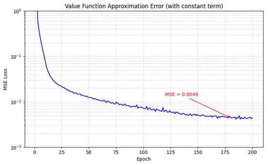
In the above, the first term is the approximation error, determined by the representational power of the neural network and the training accuracy; the second term is the iteration error, which decays exponentially due to the contraction property of the Bellman operator. Specifically, because $\mathcal{T}$ is a $\gamma -contraction$, we have ${\Vert {\widehat{V}}_k-V^{\ast }\Vert }_{\infty }\le {\gamma }^k{\Vert V_0-V^{\ast }\Vert }_{\infty }$, so the iteration error decays exponentially with $k$. The approximation error can be reduced by increasing network capacity or improving the optimisation algorithm. In the simulation experiments of this paper (Section 5.1), we verify that a neural network can approximate the Riccati analytical solution with a mean squared error of 0.0049 in the LQR setting, providing numerical confidence for the subsequent experiments on real data.

3.5. Numerical Connection Between PPO and the HJB Equation

PPO is a policy-gradient-based deep reinforcement learning algorithm. Its objective function is as follows:

$$L^{CLIP}\left(\theta \right)={\mathbb{E}}_t\left[min\left(r_t\left(\theta \right){\widehat{A}}_t,clip\left(r_t\left(\theta \right),1-ϵ,1+ϵ\right){\widehat{A}}_t\right)\right]$$

(11)

where $r_t\left(\theta \right)={\displaystyle \frac{{\pi }_{\theta }\left(a_t|s_t\right)}{{\pi }_{{\theta }_{old}}\left(a_t|s_t\right)}}$ is the probability ratio, ${\widehat{A}}_t$ is the estimated advantage function, and $ϵ$ is the clipping hyperparameter (taken as 0.2 in this paper).

The advantage function ${\widehat{A}}_t=Q(s_t,a_t)-V\left(s_t\right)$ is essentially an estimate of ${max}_a\left\{\mathcal{R}\left(s,a\right)+\gamma \mathbb{E}\left[V\left(s\prime \right)\right]\right\}-V\left(s\right)$, which appears in the HJB equation. Therefore, the policy update of PPO can be interpreted as a numerical scheme for solving the discrete HJB equation in policy space. It should be emphasised that this connection is heuristic; this paper mainly validates the feasibility of this scheme from an empirical perspective.

3.6. Algorithm Pseudocode

Algorithm 1 presents the complete workflow of the HJB-based PPO algorithm for credit decision-making, including trajectory collection, advantage estimation, policy clipping, and value function update.

Algorithm 1. HJB-based PPO Credit Decision Algorithm
Input:$\mathrm{Training} \mathrm{data} {\mathcal{D}}_{train},$ $\mathrm{test} \mathrm{data} {\mathcal{D}}_{test},$ $\mathrm{hyperparameters} \left\{\alpha ,\gamma ,ϵ,\lambda \right\}$
Output:$\mathrm{Trained} \mathrm{policy} {\pi }_{\theta }$
1	$\mathrm{Initialise} \mathrm{Actor} \mathrm{network} {\mu }_{\theta }\left(s\right)$$\mathrm{and} \mathrm{Critic} \mathrm{network} V_{\phi }\left(s\right),$$\mathrm{experience} \mathrm{replay} \mathrm{buffer} \mathcal{B}$ (note: PPO is on-policy and does not actually require a replay buffer; the buffer here is for trajectory storage)
2	for$n=1 to N$ (iterations) do
3	$\mathrm{Collect} \mathrm{trajectories} \left\{\left(s_t,a_t,r_t,s_{t+1}\right)\right\}$ $\mathrm{by} \mathrm{interacting} \mathrm{with} \mathrm{the} \mathrm{environment} \mathrm{using} \mathrm{the} \mathrm{current} \mathrm{policy} {\pi }_{{\theta }_{old}}$
4	$\mathrm{Compute} \mathrm{advantage} \mathrm{estimates} {\widehat{A}}_t=GAE\left(r,V_{\phi },\gamma ,{\lambda }_{GAE}\right)$ $\mathrm{with} {\lambda }_{GAE}=0.95$
5	for$k=1 to K$(update epochs) do
6	Sample mini-batches ${\mathcal{B}}_k$ from the collected trajectories
7	Compute the clipped objective$L^{\mathrm{C}\mathrm{L}\mathrm{I}\mathrm{P}}\left(\theta \right)$ according to Equation (11)
8	Compute Critic loss$L^{\mathrm{V}\mathrm{F}}\left(\phi \right)=\mathbb{E}\left[{\left(V_{\phi }\left(s\right)-G_t\right)}^2\right],$$\mathrm{where} G_t$ is the discounted cumulative reward
9	Update Actor:;$\theta \leftarrow \theta +\alpha {\nabla }_{\theta }{L}^{CLIP}\left(\theta \right)$
10	Update Critic: $\phi \leftarrow \phi -\alpha {\nabla }_{\phi }{L}^{VF}\left(\phi \right)$
11	end for
12	Check convergence: stop early if  ${\Vert V_{\phi }-V_{{\phi }_{old}}\Vert }_{\infty }<\delta$
13	end for
14	return${\pi }_{\theta }$

In Algorithm 1, the Critic update uses gradient descent (indicated by the minus sign) while the Actor update uses gradient ascent (plus sign). In practice, adaptive optimisers such as Adam automatically handle the signs.

4. Experimental Design and Methodology

4.1. Dataset Description

This study constructs a dynamic credit decision dataset using LendingClub loan data from 2016 to 2018 [30]. LendingClub is the largest online lending platform in the United States, and its public dataset contains detailed application information, repayment records, and final status for each loan. After rigorous data cleaning and preprocessing, the dataset contains 518,706 valid loan records, of which 402,449 are fully paid, and 116,257 are charged off, giving a default rate of approximately 22.4%. Based on the original loan data, we construct a monthly panel dataset. For each loan, we generate one record per month from the origination month until the loan is either fully paid or defaults. The final total number of observations is 21,470,544, fully capturing the dynamic risk evolution over the loan lifecycle.

The feature engineering of the dataset consists of two dimensions, as shown in Table 1.

Table 1. Variable definitions.

Dimension	Variable	Meaning
Borrower characteristics	loan_amnt	Loan amount
	int_rate	Interest rate
	dti	Debt-to-income ratio
	delinq_2yrs	Number of delinquencies in past 2 years
	revol_util	Revolving credit utilisation rate
	emp_length_num	Employment length (years)
Macroeconomic variables	unemployment_rate	Unemployment rate [31]
	fed_funds_rate	Federal funds rate [32]
	mortgage_rate	30-year mortgage rate [33]
	industrial_production	Industrial production index [34]
	cpi	Consumer price index [35]

All macroeconomic variables are aligned to the monthly panel data at a monthly frequency. Missing values are handled by forward filling and overall mean imputation. Additionally, the dataset contains auxiliary columns: loan_id (unique loan identifier), month (month), loan_status (Fully Paid or Charged Off), and reward_scaled (scaled reward value).

The data are split temporally following strict forward validation principles:

• Training set: January 2016 to December 2017, totalling 6,817,877 time steps.
• Test set: January 2018 to December 2018, totalling 6,011,950 time steps.

This split ensures that the loans in the test set occur strictly after the training period in time, preventing data leakage.

4.2. Environment Construction and Counterfactual Assumption

Each episode corresponds to the full lifecycle of a single loan. At environment initialisation, a loan is randomly sampled from the training-set loan ID pool. The environment then returns states month by month in chronological order. At each time step, the environment provides the current state (11 normalised features); the agent outputs an action (credit ratio $a_t\in [0, 1]$), the environment computes the immediate reward and returns the next state. The episode terminates when the loan status becomes “Fully Paid” or “Charged Off”.

The state transition is implemented as follows: given the current state $s_t$ and action $a_t$, the environment looks up the real observation at the next time step for that loan ID in the historical data and returns it as $s_{t+1}$. A critical issue arises: when the policy’s output $a_t$ differs from the historical action (i.e., the actual credit behaviour that occurred in that month—note that the raw data contain only the initial credit limit set at loan origination and no subsequent adjustments), how do we define the next state? Since the credit limit in LendingClub data is fixed at origination and never changed thereafter, the historical action is implicitly defined: For a fully paid loan, we may consider the historical action to be $a=1$ (full credit); for a defaulted loan, we may consider the historical action to be $a=0$ (complete rejection). However, this is clearly an oversimplified assumption.

To address this dilemma, this paper adopts an implicit one-step counterfactual assumption: we treat the environment as an empirical simulator—the state transition function directly reuses the historically observed subsequent state, irrespective of whether the action matches. That is, regardless of the action taken by the agent, the next state is fixed to the real state of that loan at the next time step in the history. The justification is that we are not trying to answer the causal question “how would the borrower’s behaviour change if we changed the credit limit?”. Instead, we formulate the task as learning an optimal credit policy from historical data, where the historical data reflect a fixed credit rule (typically full credit). The policy learned by PPO can be interpreted as: under the distribution of historical trajectories, how should the credit ratio be adjusted to maximise cumulative reward? This approach avoids complex causal inference, but when the policy deviates significantly from the historical action, the estimates may be biased. To mitigate this, we add a quadratic penalty term $\lambda a_t^2$ to the reward function to discourage the policy from deviating too far from $a_t=0$ (i.e., to avoid excessively high credit), and we also use PPO’s clipping mechanism to limit the magnitude of policy updates.

4.3. Feature Normalisation and Data Leakage Prevention

To ensure training stability, all features are normalised before being fed into the network:

$$\tilde{s}={\displaystyle \frac{s-\mu }{\sigma }}$$

(12)

where $\mu$ and $\sigma$ are the mean and standard deviation computed from the first 10,000 samples of the training set. These parameters are computed once at the beginning of training and then fixed throughout training and evaluation. The test set uses the same $\mu$ and $\sigma$; no statistics from the test set are used. Moreover, there is no overlap in loan IDs between the training and test sets, and the temporal split ensures no future information leakage.

4.4. Reward Function Design

The design of the reward function is central to the reinforcement learning framework. We define the immediate reward as follows:

$$\mathcal{R}\left(s_t,a_t\right)={reward\_scaled}_t\cdot a_t-\lambda a_t^2$$

(13)

where

• ${\mathrm{reward}\_\mathrm{scaled}}_t$: the base reward. For months with normal repayment, it equals the monthly interest income divided by 1000 (numerical scaling); for the last month of a defaulted loan, it equals (monthly interest − loan principal) divided by 1000. The scaling brings the reward magnitude into a range of about several tens, which is beneficial for neural network training.
• $a_t\in [0, 1]$: the credit ratio output by the agent.
• $\lambda =0.01$: the quadratic penalty coefficient, used to penalise excessive credit and to encourage the policy to reduce the credit ratio when risk is high.

When a borrower repays normally, ${\mathrm{reward}\_\mathrm{scaled}}_t>0$, so the reward increases linearly with $a_t$ but is also penalised by the quadratic term, giving an optimal $a_t^{\ast }={\displaystyle \frac{{reward\_scaled}_t}{2\lambda }}$ (capped at 1 if this value exceeds 1). When a borrower defaults, ${\mathrm{reward}\_\mathrm{scaled}}_t$ is negative, and the reward encourages $a_t$ to be as small as possible, i.e., to reduce credit and limit losses.

4.5. Experimental Environment and Model Architectures

Experiments are conducted on the AutoDL platform. Hardware: 4× NVIDIA RTX 5090 GPUs, AMD EPYC 7542 CPU (25 cores/GPU), 90 GB RAM/GPU. Software: Python 3.12, PyTorch 2.8.0 (CUDA 12.8), gymnasium 0.29.1, stable-baselines3 2.4.0, scikit-learn 1.5.0, XGBoost 2.1.0, LightGBM 4.5.0.

PPO model uses the MlpPolicy from the stable-baselines3 library. The Actor-Critic network shares a common feature extraction layer consisting of two hidden layers with 64 neurons each and ReLU activation. The Actor output layer outputs the mean and standard deviation of the action, using a Gaussian distribution to parameterise the continuous action space; the action range is mapped to $\left[0, 1\right]$ via a tanh function. The Critic output layer outputs a scalar state value estimate. Training hyperparameters: learning rate $3\times {10}^{-4}$, total time steps 5,000,000, GAE parameter ${\lambda }_{\mathrm{GAE}}=0.95$, clipping range $ϵ=0.2$, batch size 64, number of update epochs 10. To assess stability, training is performed with four different random seeds, and the reported results are averages over these runs.

PPO linear variant (PPO_linear) uses policy_kwargs=dict(net_arch=[]), i.e., the policy network has no hidden layers and directly maps the input to the output.

DQN model serves as another reinforcement learning baseline, using a discrete action space (11 discrete actions corresponding to 0.0, 0.1, …, 1.0). The network has two hidden layers with 64 neurons each. Hyperparameters: learning rate $1\times {10}^{-4}$, total time steps 5,000,000, replay buffer size 500,000, learning starts after 50,000 steps, batch size 128, target network update interval 10,000.

Static baseline models are summarised in Table 2.

Table 2. Static baseline model architectures and hyperparameters.

Model	Architecture and Hyperparameters
LR	max_iter = 1000
RF	n_estimators = 300, max_depth = 20, min_samples_split = 20
XGBoost	n_estimators = 300, learning_rate = 0.05, max_depth = 6, subsample = 0.8, colsample_bytree = 0.8
LightGBM	n_estimators = 300, learning_rate = 0.05, num_leaves = 31
MLP	hidden_layer_sizes = (128, 64), max_iter = 200, early_stopping = True
Stacked_Meta-Model	Base learners: RF, XGBoost, MLP; meta-learner: logistic regression; meta-features generated via cross-validation.

All static models output a default probability $P$, which is then converted to a continuous action $a=1-P$ to enable comparison with PPO on the same metrics.

For ablation studies, in addition to PPO_linear, we also evaluate a random policy (actions uniformly sampled from $\left[0, 1\right]$) and a constant policy (action fixed at 0.5); these require no training.

4.6. Evaluation Metrics

This study designs two sets of evaluation metrics—dynamic profit metrics and static classification metrics—to comprehensively assess model performance across different dimensions.

Dynamic profit metrics evaluate the long-term profitability of models on the LendingClub test set. These metrics directly reflect the models’ profitability and risk control ability in real credit decisions.

• Average Reward (AvgReward) is the arithmetic mean of the cumulative rewards over all test samples, reflecting the model’s average profit per loan:

$$AvgReward={\displaystyle \frac{1}{N}}{\displaystyle \sum _{i=1}^N}{R}_i$$

(14)

• Total Reward (TotalReward) is the sum of cumulative rewards over all test samples, giving an intuitive measure of overall profitability:

$$TotalReward={\displaystyle \sum _{i=1}^N}{R}_i$$

(15)

• Standard deviation of reward (Std) measures the volatility of the model’s rewards, defined as the standard deviation of the cumulative reward per loan:

$$Std=\sqrt{{\displaystyle \frac{1}{N}}{\displaystyle \sum _{i=1}^N}{\left(R_i-AvgReward\right)}^2}$$

(16)

• Sharpe ratio measures excess return per unit of total risk, a widely used risk-adjusted return metric in finance:

$$Sharpe={\displaystyle \frac{E\left[R\right]-R_f}{{\sigma }_R}}$$

(17)

where $R_f$ is the risk-free rate (taken as 0 in this paper) and ${\sigma }_R$ is the standard deviation of rewards.

• Sortino ratio improves upon the Sharpe ratio by penalising only downside risk, better reflecting the model’s ability to control losses [36]:

$$Sortino={\displaystyle \frac{E\left[R\right]-R_f}{{\sigma }_{down}}}$$

(18)

where ${\sigma }_{\mathrm{down}}$ is the standard deviation of negative rewards (downside risk).

• Invalid action rate assesses the rationality of the model’s decisions, defined as the proportion of actions that either grant a high credit limit (>0.5) to high-risk borrowers or grant a low credit limit (<0.5) to low-risk borrowers:

$$InvalidRate={\displaystyle \frac{1}{N}}{\displaystyle \sum _{i=1}^N}\left[\left(y_i=1\wedge a_i>0.5\right)\vee \left(y_i=0\wedge a_i<0.5\right)\right]$$

(19)

The threshold of 0.5 is chosen as the natural midpoint between complete rejection (0) and full credit (1). In credit scoring practice, a binary decision is often made by comparing a risk score against a cutoff; here, the continuous action $a_t$ represents the credit ratio, and values above 0.5 indicate a “high-credit” approval while values below 0.5 indicate a “low-credit” or “restricted” decision. The 0.5 threshold thus serves as a neutral reference to evaluate whether the model’s continuous recommendation is directionally consistent with the borrower’s risk level (high-risk borrowers should receive low credit, and vice versa). This definition of invalid action rate follows the common practice in the literature when discretising continuous policy outputs for interpretability.

Static classification metrics evaluate model performance on the Give Me Some Credit dataset [37]. These metrics are based on the confusion matrix (see Table 3).

Table 3. Confusion matrix.

Actual Class	Predicted Default (1)	Predicted Non-Default (0)
Default (1)	True Positive (TP)	False Negative (FN)
Non-Default (0)	False Positive (FP)	True Negative (TN)

• AUC (Area Under the ROC Curve) measures the model’s ability to distinguish between positive and negative classes; values closer to 1 indicate better classification performance.
• Accuracy is the proportion of correctly predicted samples:

$$ACC={\displaystyle \frac{TP+TN}{TP+TN+FP+FN}}$$

(20)

• F1 score is the harmonic mean of precision and recall, providing a more informative metric than accuracy under imbalanced conditions:

$$F1=2\cdot {\displaystyle \frac{Precision\cdot Recall}{Precision+Recall}}, Precision={\displaystyle \frac{TP}{TP+FP}}, Recall={\displaystyle \frac{TP}{TP+FN}}$$

(21)

• Sensitivity (Recall) measures the ability to identify default samples:

$$Sens={\displaystyle \frac{TP}{TP+FN}}$$

(22)

• Specificity measures the ability to identify non-default samples:

$$Spec={\displaystyle \frac{TN}{TN+FP}}$$

(23)

5. Experimental Results and Analysis

5.1. Theoretical Numerical Validation

To verify the feasibility of using a neural network as a numerical solver for the HJB equation, we perform a simulation experiment following the setup of Section 3.4. Set the system matrices $A,B$ as described above, $Q=I_3$, $R=1$, $\lambda =0.01$, $\mathsf{\Sigma }=0.1I_3$, $\gamma =0.99$. Solving the Riccati equation gives the positive definite matrix $P$ and the constant term $c$:

$$P=\left[\begin{array}{ccc}4.3261& 1.0055& 0.1480\\ 1.0055& 3.1636& 0.5724\\ 0.1480& 0.5724& 2.1659\end{array}\right], c=95.5896$$

We then generate 10,000 trajectories of length 24 and train a three-layer neural network (input dimension 3, hidden layers 64–64, output dimension 1) to fit $V\left(s\right)=-s^{\mathrm{T}}Ps-c$.

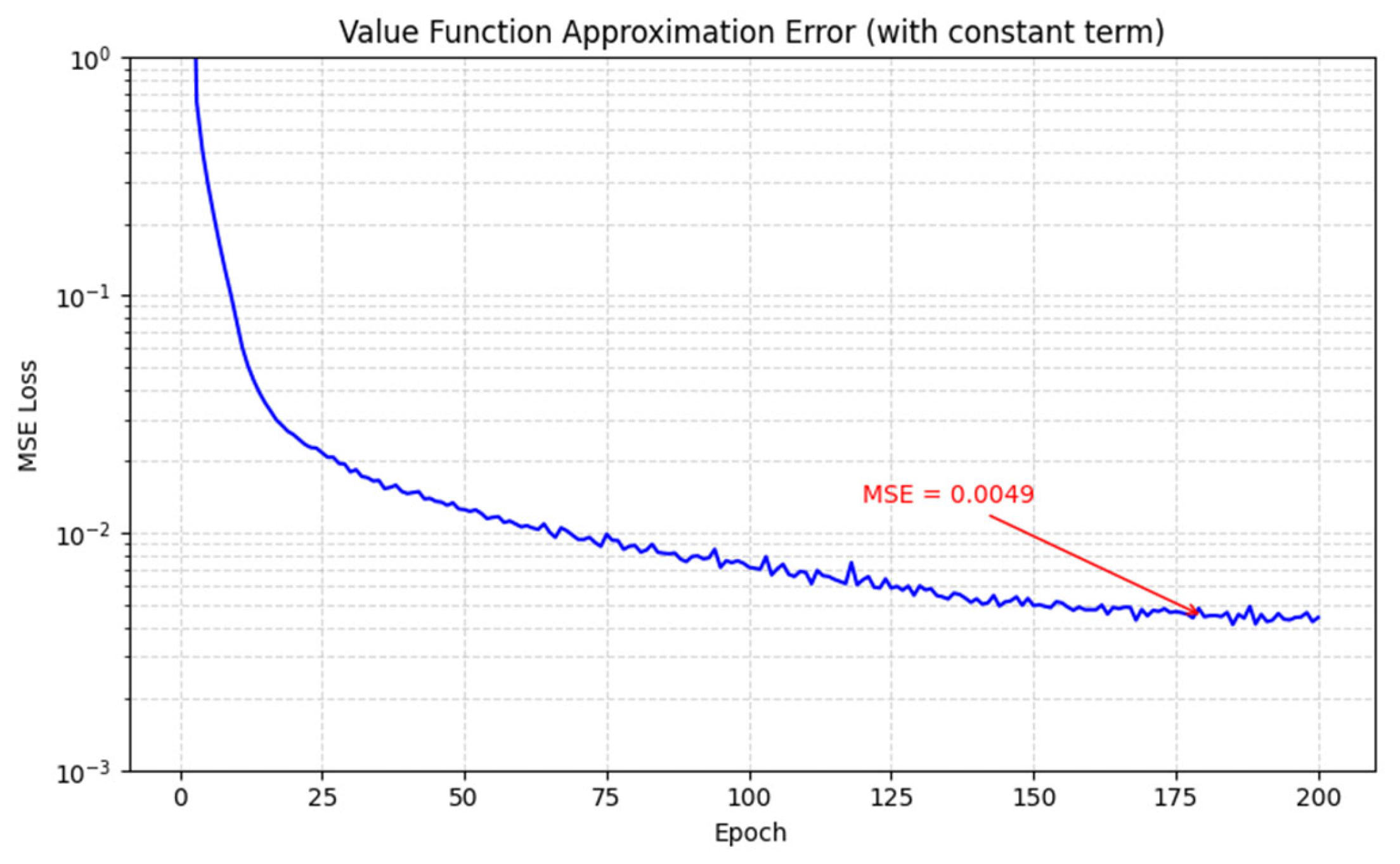
Figure 1 shows the loss curve. The initial loss is about 0.0125 and decreases to 0.0049 after 200 training epochs. This extremely low approximation error indicates that a neural network can fit the Riccati analytical solution with high precision. This result numerically supports the feasibility of neural network value iteration as an effective numerical scheme for the HJB equation: even in the idealised linear-quadratic world, a neural network achieves satisfactory approximation accuracy, providing confidence for applying the PPO algorithm to complex real-world data.

Figure 1. Theoretical validation loss curve (epoch vs. MSE loss; curve decreases from 0.0125 to 0.0049).

5.2. Dynamic Profit Performance Comparison

Table 4 summarises the dynamic profit metrics of all models on the LendingClub test set.

Table 4. Dynamic profit performance comparison.

Model	$\mathbf{A}\mathbf{v}\mathbf{g}\mathbf{R}\mathbf{e}\mathbf{w}\mathbf{a}\mathbf{r}\mathbf{d} \pm \mathbf{S}\mathbf{t}\mathbf{d}$	TotalReward	Sharpe	Sortino	InvalidRate
PPO (multiple seeds)	$1.6726\pm 1.8819$	$8.6761\times {10}^5$	0.8888	1.7722	0.2542
LR	$1.3023\pm 1.3687$	$6.7552\times {10}^5$	0.9515	1.4936	0.2296
RF	$1.3039\pm 1.2746$	$6.7633\times {10}^5$	1.0230	1.9164	0.1731
XGBoost	$1.2931\pm 1.3634$	$6.7074\times {10}^5$	0.9484	1.5287	0.2234
LightGBM	$1.2917\pm 1.3603$	$6.7001\times {10}^5$	0.9496	1.5338	0.2242
MLP	$1.3209\pm 1.3853$	$6.8515\times {10}^5$	0.9535	1.5420	0.2254
Stacked_Meta-Model	$1.3382\pm 1.4665$	$6.9413\times {10}^5$	0.9125	8.3308	0.0574
DQN	$1.5334\pm 1.9540$	$7.9539\times {10}^5$	0.7848	1.7795	0.3438

PPO achieves the highest average reward (1.6726) and total reward (867,613), significantly surpassing all static models and DQN. However, its reward standard deviation (1.8819) is also the highest among all models, indicating that while PPO pursues high expected returns, it also accepts larger reward volatility. This reflects the essential difference between PPO and static models: PPO prioritises profit maximisation and is willing to accept higher volatility in exchange for higher expected returns; static models, in contrast, tend to take extreme decisions (credit ratios close to 0 or 1) to reduce the probability of negative returns, thereby suppressing volatility but also sacrificing many positive-return opportunities.

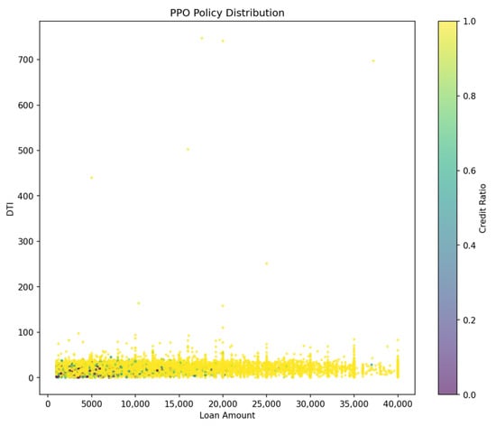
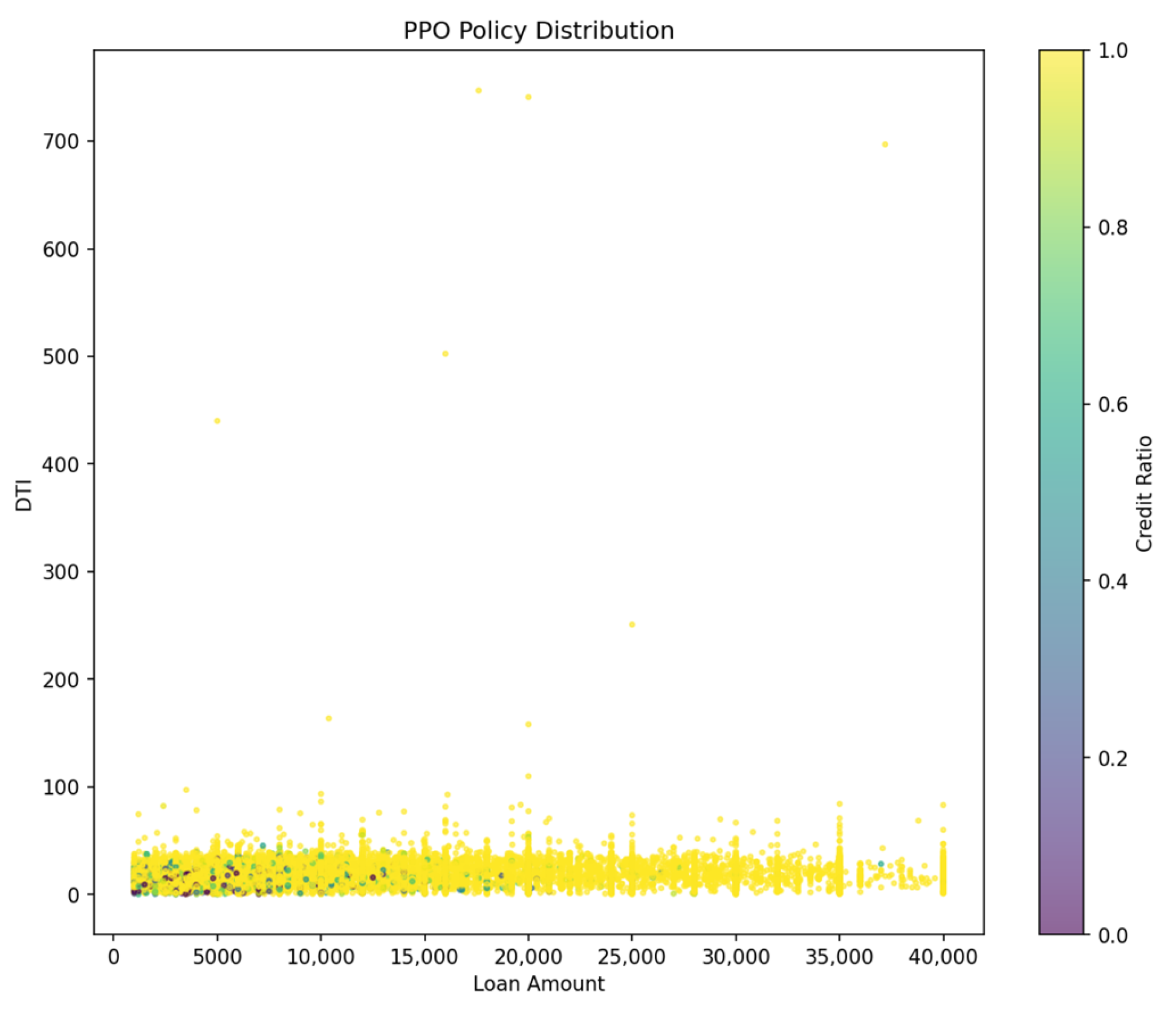
Figure 2 shows the credit ratio distribution of the PPO policy on the test set. The horizontal axis is loan amount, and the vertical axis is debt-to-income ratio (DTI). It can be observed that most samples concentrate in the low-DTI region, where credit ratios are generally high, indicating that the model tends to grant full credit to low-risk customers. High-DTI regions are sparser, consistent with the smaller number of borrowers with high debt-to-income ratios in the dataset; even in those regions, credit ratios remain predominantly high. This distribution reflects the model’s decision tendency—guided by the reward function—to maximise long-term cumulative profit: in most cases it chooses high credit to obtain positive returns, while the quadratic penalty prevents excessive credit that could lead to large losses. It is worth noting that because the environment is built using historical trajectory reuse rather than a causal counterfactual transition, the model does not learn a feedback-regulation behaviour such as “reducing credit would improve the borrower’s future state”. Nevertheless, even under this limitation, PPO still achieves significantly higher returns than all static baselines, which demonstrates the core advantage of global sequential optimisation.

Figure 2. Policy distribution scatter plot (loan amount vs. DTI, colour indicates credit ratio).

DQN has a higher average reward than all static models but is still lower than PPO, and its standard deviation is slightly larger than that of PPO. As a value-function method with a discrete action space (11 discrete values), DQN’s approximation is limited, which prevents it from achieving the fine-grained adjustments possible with continuous actions, resulting in somewhat lower returns than PPO. Moreover, DQN’s invalid action rate is significantly higher than that of PPO, indicating that DQN more often incorrectly assigns high credit limits to high-risk customers, possibly due to the discrete action space’s insufficient ability to fit the risk-return boundary.

An interesting observation is that RF has a higher Sortino ratio (1.9164) than PPO (1.7722), and even RF’s Sharpe ratio (1.023) is significantly higher than PPO’s (0.8888). This might appear to suggest that RF is better on a risk-adjusted basis, but we must look at the average reward: RF’s average reward is only 1.3039, which is 22% lower than PPO’s. RF achieves a high Sortino ratio because its predicted probabilities are extreme, leading to actions that are almost always 0 or 1, so negative returns are very rare (downside risk is very small). However, this extreme strategy comes at the cost of sacrificing many positive-return opportunities: although RF often grants near-full credit to low-risk customers, it cannot, like PPO, give moderate credit ratios to medium-risk customers to balance risk and return. Therefore, PPO’s large advantage in absolute returns more than compensates for its slightly higher downside volatility, which aligns better with a financial institution’s goal of profit maximisation.

The stacked meta-model exhibits an extremely high Sortino ratio of 8.33, far exceeding all other models. Inspection of its reward distribution reveals that the stacked meta-model tends to give very high credit ratios (median 0.9941). This strategy results in 99.13% of samples having positive returns and only 0.60% having negative returns, with a downside standard deviation of only 0.1606. Although the Sortino ratio is numerically very high, the underlying reason is not that the model has superior risk-adjustment ability, but rather that it almost never produces negative returns—achieved by almost always granting near-full credit. However, its average reward is still far below that of PPO, demonstrating that “avoiding negative returns” is not equivalent to “maximising profit”. PPO accepts moderate downside risk in exchange for higher expected returns. Hence, the Sortino ratio alone can be misleading and must be interpreted together with the average reward and the action distribution.

5.3. Static Classification Performance Comparison

It should be noted that PPO, as a dynamic decision-making model designed to maximise the cumulative reward over the loan lifecycle, has a fundamentally different objective from static classification and therefore should not be directly compared on static metrics. Table 5 lists the classification performance of the static baseline models on the Give Me Some Credit dataset. Among these, XGBoost achieves the highest AUC, while LightGBM achieves the highest accuracy. The stacked meta-model performs prominently in F1 score and sensitivity, thanks to its ensemble structure that better captures patterns of the minority class (default). The models show trade-offs across different metrics, reflecting the inherent tensions in imbalanced classification tasks. Nevertheless, these results confirm that the static baselines considered in this study all achieve a consistently high level of performance on the traditional default prediction task. This, in turn, underscores the value of PPO’s dynamic profit advantage—it does not simply outperform weak baselines but surpasses already strong and widely recognised static models, further reinforcing the practical significance of the dynamic decision-making framework.

Table 5. Static classification performance comparison.

Model	AUC	ACC	F1-Score	Sens	Spec
LR	0.6844	0.9312	0.0882	0.0479	0.9979
RF	0.8439	0.9334	0.2764	0.1831	0.9894
XGBoost	0.8493	0.9334	0.2810	0.1873	0.9891
LightGBM	0.8484	0.9337	0.2825	0.1879	0.9894
MLP	0.8106	0.9329	0.2782	0.1861	0.9887
Stacked_Meta-Model	0.7808	0.9222	0.3233	0.2675	0.9711

5.4. Ablation Experiments

Table 6 presents the results of the ablation experiments. Replacing the nonlinear policy network of PPO with a linear mapping (PPO_linear) causes the average reward to drop sharply from 1.6726 to 0.9902, a reduction of 40.8%. Both the random policy (actions uniformly sampled) and the constant policy (action fixed at 0.5) yield average rewards below 1.0, further indicating that an unlearned policy cannot accumulate profits effectively.

Table 6. Ablation experiment results.

Model	AvgReward	TotalReward
PPO (multiple seeds)	1.6726	$8.6761\times {10}^5$
PPO_linear	0.9902	$5.1364\times {10}^5$
Random Policy	0.9272	$4.8094\times {10}^5$
Constant 0.5	0.9266	$4.8063\times {10}^5$

Although the linear policy’s return is far below that of PPO, it is still higher than the random and constant policies, indicating that even without nonlinear expressive power, the learned linear mapping can capture some basic risk-return relationships, e.g., customers with higher default probabilities receive lower credit ratios. However, a linear boundary cannot capture complex interactions between features (e.g., the nonlinear effect when high DTI and high interest rate occur together) nor achieve fine-grained regional differentiation. This ablation result supports the assertion of Theorem 3: nonlinear function approximation is key to using neural network value iteration to approximate the solution of the HJB equation.

5.5. Reward Distribution and Boxplot Analysis

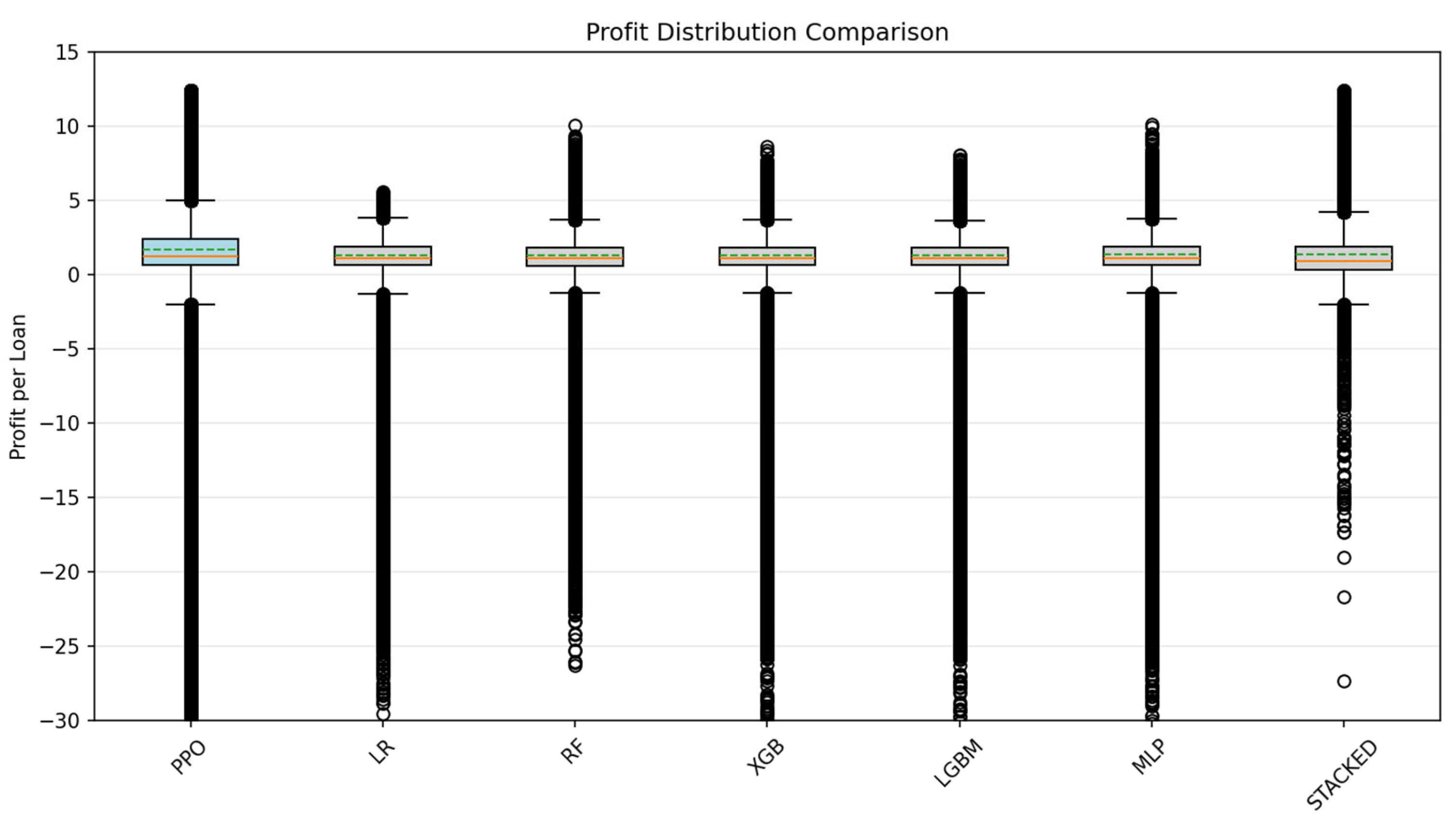
The boxplots in Figure 3 visually depict the distribution of per-loan rewards on the test set for PPO and each static model. From the plots, it is clear that PPO’s box is positioned higher overall, with its median line noticeably above those of other models; its right whisker is longer, and there are more outliers in the high-reward region (e.g., points far above the boxes in Figure 3). These visual cues suggest that PPO may have a systematic advantage in reward distribution. To quantitatively characterise the distributional features and validate the visual observations, Table 7 summarises the medians, quartiles, and extremes of the rewards for each model.

Figure 3. Boxplots of reward distributions for PPO vs. each static model. Within each box, the dashed line represents the mean, the solid line represents the median, and the small circles outside the boxes indicate outliers.

Table 7. Reward distribution statistics for each model.

Model	Median	Max	Min	Q1	Q3
PPO (multiple seeds)	1.2253	12.3960	−32.6244	0.6118	2.3666
LR	1.1093	5.5674	−29.5876	0.5995	1.8808
RF	1.0718	10.0147	−26.3482	0.5943	1.8227
XGBoost	1.0787	8.5832	−30.8519	0.5994	1.8214
LightGBM	1.0781	8.0483	−30.8003	0.5992	1.8171
MLP	1.1103	10.1205	−30.8089	0.6170	1.8616
Stacked_Meta-Model	0.9106	12.3960	−27.3556	0.3216	1.8749

From the box positions in Figure 3 and the median data in Table 7, PPO’s median reward reaches 1.2253, significantly higher than all static models, with a lead ranging from about 0.1 to 0.3. This advantage is visually evident in Figure 3 as the median line (the horizontal line inside the box) of PPO’s box being notably higher than those of other models. For the upper quartile (Q3), PPO also leads with 2.3666, reflected in Figure 3 as the upper half of PPO’s box being generally higher, indicating that even among the best-performing 25% of samples, PPO’s rewards are more outstanding. This result aligns with the average reward advantage in Section 5.2 and is more robust to extreme values.

The tail characteristics of the reward distribution are particularly striking in Figure 3. PPO’s right whisker is significantly longer than those of other models, and there are multiple outliers far above the upper bounds of other models’ boxes. Table 7 confirms this: PPO’s maximum (12.3960) is close to that of the stacked meta-model but clearly higher than other models, while its upper quartile and median are also clearly superior. This means that PPO’s high rewards are not reliant on isolated extreme values but are generally superior in the high-reward region. Combined with the density distribution of PPO’s right tail in Figure 3, we can infer that its high-reward samples are denser, directly reflecting the ability of its dynamic strategy to capture excess profits from high-quality customers.

In terms of downside risk, except for RF and the stacked meta-model, the left whiskers of the models in Figure 3 are similar in length, and the lower quartiles show little difference, further corroborated by the data in Table 7. PPO’s minimum is −32.6244, slightly lower than other models. Although it does not minimise negative profits, given its higher median and upper quartile, this risk exposure is reasonable—PPO trades manageable downside risk for far greater upside returns than static models. This characteristic precisely reflects the difference in objectives between dynamic decision models and static classification models: the former prioritises profit maximisation and is willing to accept some volatility in pursuit of higher expected returns, while the latter tends to avoid risk through conservative decisions, thereby sacrificing substantial potential profits.

Considering the visual forms in Figure 3 and the statistics in Table 7, PPO’s reward distribution exhibits an “overall right shift with a heavier right tail”. This distribution not only stochastically dominates static models in a probabilistic sense but also implies, in practical business terms, more stable profitability and a broader surplus profit space. The coordinated analysis of boxplots and statistical tables provides a complete evidentiary chain for understanding PPO’s reward advantages, ranging from global patterns to local details and from intuition to quantification.

5.6. Sensitivity Analysis and Statistical Significance Testing

To assess the robustness of the model to hyperparameters, we train PPO models with different combinations of the penalty coefficient $\lambda \in \left\{\mathrm{0.001,0.01,0.05}\right\}$ and the discount factor $\gamma \in \left\{\mathrm{0.95,0.99,1.00}\right\}$ using the default seed, and compute the average reward on the test set. The results are shown in Table 8.

Table 8. Sensitivity analysis results.

$\mathit{\lambda }$	$\mathit{\gamma }$	AvgReward
0.001	0.95	1.6689
0.001	0.99	1.6361
0.001	1.00	1.8531
0.01	0.95	1.8433
0.01	0.99	1.8532
0.01	1.00	1.7320
0.05	0.95	1.6367
0.05	0.99	1.8406
0.05	1.00	1.6834

From Table 8, all nine hyperparameter combinations yield average rewards above 1.6, with the highest reaching 1.8532, and all nine results are higher than those of all static baselines. This indicates that PPO is not sensitive to hyperparameter choices and has good robustness.

Furthermore, to test whether the difference between PPO and the strongest static baseline is statistically significant, we perform independent two-sample t-tests. Taking XGBoost as a representative static baseline, we compare the per-loan reward array of PPO with that of XGBoost and obtain a p-value of 0.0000. Similarly, the t-test between PPO and the stacked meta-model also gives a p-value of 0.0000. Therefore, we can confidently state that PPO’s reward advantage in the dynamic credit decision task is statistically significant and not due to random fluctuations.

6. Conclusions

This paper liberates credit scoring from the constraints of static classification, places it within the mathematical framework of stochastic optimal control, and provides a reproducible empirical implementation based on real data. Theoretically, we reviewed standard results for discrete MDPs and the HJB equation, derived the closed-form Riccati solution under linear-quadratic assumptions, including the constant term due to noise, and verified the feasibility of numerical solution via neural network value iteration experiments. These classical tools are systematically integrated into a dynamic optimisation framework for credit decision-making for the first time, establishing a theoretical benchmark for the subsequent empirical work.

Empirically, using real LendingClub loan data from 2016–2018, the PPO model trained in this paper significantly outperforms static baselines such as logistic regression, random forest, XGBoost, as well as the DQN baseline, in both average reward and total reward, and the reward distribution exhibits a pattern of “overall right shift and heavier right tail”. Ablation studies show that the nonlinear policy achieves 68.9% higher average reward than the linear policy, while the random and constant policies both yield rewards below 1.0, demonstrating the necessity of nonlinear function approximation and sequential decision learning. In sensitivity analysis, all nine hyperparameter combinations give average rewards above 1.6, and statistical tests confirm the significance of PPO’s advantage (p < 0.001).

The main contributions of this paper are threefold and interrelated.

• Theoretical integration: For the first time, we systematically embed classical tools—the Bellman optimality equation for discrete MDPs, the closed-form Riccati solution for LQR problems, and the error decomposition for neural network value iteration—into a dynamic control framework for credit scoring. By explicitly deriving the analytical solution, including the constant term under linear-quadratic assumptions and providing a numerical benchmark for neural network approximation, we bridge the gap between abstract control theory and practical credit decisions, making mature methods from optimal control directly applicable to financial risk management.
• Empirical breakthrough: Using a large-scale real loan dataset, we demonstrate for the first time that the HJB-PPO framework achieves a dominant advantage (25% higher average reward) over the strongest static baselines on dynamic profit metrics. This result is not obtained by comparing against weak baselines; it surpasses widely recognised models such as logistic regression, XGBoost, and stacked ensemble models, providing the industry with a reproducible performance benchmark and engineering reference.
• Methodological inspiration: Through ablation experiments including linear, random, and constant policies, we quantitatively reveal the critical role of nonlinear function approximation in credit decisions. Sensitivity analysis over nine hyperparameter combinations shows the model’s robustness under different penalty coefficients and discount factors, and significance testing confirms the statistical credibility of the advantage. These systematic experiments not only validate the framework but also provide a template for evaluation that future researchers can follow.

The framework presented here clearly demonstrates the profit potential of shifting from static classification to dynamic optimisation. Looking ahead, causal environment modelling, portfolio-level risk hedging (e.g., CVaR), multi-agent collaborative decision-making, and model interpretability are key directions for extending this framework toward practical deployment. This paper provides a solid theoretical and empirical foundation for applying reinforcement learning in financial risk control and opens a viable path for the intelligent transformation of credit decision-making.

References

- Dastile, X.; Celik, T.; Potsane, M. Statistical and machine learning models in credit scoring: A systematic literature survey. Appl. Soft Comput. 2020, 91, 106263. [Google Scholar] [CrossRef] [Scilit]
- Li, Y.H.; Chen, W.D. A Comparative Performance Assessment of Ensemble Learning for Credit Scoring. Mathematics 2020, 8, 1756. [Google Scholar] [CrossRef] [Scilit]
- Melo, L., Jr.; Nardini, F.M.; Renso, C.; Trani, R.; Macedo, J.A. A novel approach to define the local region of dynamic selection techniques in imbalanced credit scoring problems. Expert Syst. Appl. 2020, 152, 113351. [Google Scholar] [CrossRef] [Scilit]
- Cubiles-De-La-Vega, M.D.; Blanco-Oliver, A.; Pino-Mejías, R.; Lara-Rubio, J. Improving the management of microfinance institutions by using credit scoring models based on Statistical Learning techniques. Expert Syst. Appl. 2013, 40, 6910–6917. [Google Scholar] [CrossRef] [Scilit]
- Ito, K.; Reisinger, C.; Zhang, Y.F. A Neural Network-Based Policy Iteration Algorithm with Global H2-Superlinear Convergence for Stochastic Games on Domains. Found. Comput. Math. 2021, 21, 331–374. [Google Scholar] [CrossRef] [Scilit]
- Chen, Y.J.; Calabrese, R.; Martin-Barragan, B. Interpretable machine learning for imbalanced credit scoring datasets. Eur. J. Oper. Res. 2024, 312, 357–372. [Google Scholar] [CrossRef] [Scilit]
- Columba, F.; Cugliari, M.; Di Virgilio, S. Credit Risk Assessment with Stacked Machine Learning. In Corporate Credit Analysis and AI: Advancing the Rating System at a Central Bank; Scalia, A., Ed.; Springer Nature: Cham, Switzerland, 2026; pp. 263–292. [Google Scholar]
- Ayari, H.; Guetari, P.R.; Kraïem, P.N. Machine learning powered financial credit scoring: A systematic literature review. Artif. Intell. Rev. 2025, 59, 13. [Google Scholar] [CrossRef] [Scilit]
- Krasheninnikova, E.; García, J.; Maestre, R.; Fernández, F. Reinforcement learning for pricing strategy optimization in the insurance industry. Eng. Appl. Artif. Intell. 2019, 80, 8–19. [Google Scholar] [CrossRef] [Scilit]
- Taghian, M.; Asadi, A.; Safabakhsh, R. Learning financial asset-specific trading rules via deep reinforcement learning. Expert Syst. Appl. 2022, 195, 116523. [Google Scholar] [CrossRef] [Scilit]
- Dang, T.K.; Tran, T.C.; Tuan, L.M.; Tiep, M.V. Machine Learning Based on Resampling Approaches and Deep Reinforcement Learning for Credit Card Fraud Detection Systems. Appl. Sci. 2021, 11, 10004. [Google Scholar] [CrossRef] [Scilit]
- Paul, S.; Gupta, A.; Kar, A.K.; Singh, V. An Automatic Deep Reinforcement Learning based Credit Scoring Model using Deep-Q Network for Classification of Customer Credit Requests. In Proceedings of the 29th Annual IEEE International Symposium on Technology and Society, Swansea, UK, 13–15 September 2023. [Google Scholar]
- Zhang, K.; Yang, X.Q.; Hu, Y.H. Power penalty method for solving HJB equations arising from finance. Automatica 2020, 111, 108668. [Google Scholar] [CrossRef] [Scilit]
- Munos, R. A study of reinforcement learning in the continuous case by the means of viscosity solutions. Mach. Learn. 2000, 40, 265–299. [Google Scholar] [CrossRef] [Scilit]
- Mohammadi, H.; Zare, A.; Soltanolkotabi, M.; Jovanovic, M.R. Convergence and Sample Complexity of Gradient Methods for the Model-Free Linear-Quadratic Regulator Problem. IEEE Trans. Autom. Control 2022, 67, 2435–2450. [Google Scholar] [CrossRef] [Scilit]
- Lessmann, S.; Baesens, B.; Seow, H.V.; Thomas, L.C. Benchmarking state-of-the-art classification algorithms for credit scoring: An update of research. Eur. J. Oper. Res. 2015, 247, 124–136. [Google Scholar] [CrossRef] [Scilit]
- Ala’raj, M.; Abbod, M.F. Classifiers consensus system approach for credit scoring. Knowl.-Based Syst. 2016, 104, 89–105. [Google Scholar] [CrossRef] [Scilit]
- Perrusquía, A. Solution of the linear quadratic regulator problem of black box linear systems using reinforcement learning. Inf. Sci. 2022, 595, 364–377. [Google Scholar] [CrossRef] [Scilit]
- Li, N.; Li, X.; Peng, J.; Xu, Z.Q. Stochastic Linear Quadratic Optimal Control Problem: A Reinforcement Learning Method. IEEE Trans. Autom. Control. 2022, 67, 5009–5016. [Google Scholar] [CrossRef] [Scilit]
- Shao, J.H.; Mitra, S.; Karathanasopoulos, A. Optimal feedback control of stock prices under credit risk dynamics. Ann. Oper. Res. 2022, 313, 1285–1318. [Google Scholar] [CrossRef] [Scilit]
- Park, J.; Yi, D.; Ji, S. A Novel Learning Rate Schedule in Optimization for Neural Networks and It’s Convergence. Symmetry 2020, 12, 660. [Google Scholar] [CrossRef] [Scilit]
- Zhang, H.S.; Zhang, C.; Wu, W. Convergence of Batch Split-Complex Backpropagation Algorithm for Complex-Valued Neural Networks. Discret. Dyn. Nat. Soc. 2009, 2009, 329173. [Google Scholar] [CrossRef] [Scilit]
- Jin, F.; Cheng, K.Y.; Xie, X.L.; Chen, S.B. Robust Optimal Reinsurance and Investment Problem Under Markov Switching via Actor-Critic Reinforcement Learning. Mathematics 2025, 13, 3502. [Google Scholar] [CrossRef] [Scilit]
- Hu, N.T.; Kao, H.T.; Chen, C.S.; Chang, S.H. Actor-Critic Trajectory Controller with Optimal Design for Nonlinear Robotic Systems. Cmc-Comput. Mater. Contin. 2026, 87, 83. [Google Scholar] [CrossRef] [Scilit]
- Wu, Q.Y.; Wu, Y.H.; Wang, Y.H. Integral Reinforcement-Learning-Based Optimal Containment Control for Partially Unknown Nonlinear Multiagent Systems. Entropy 2023, 25, 221. [Google Scholar] [CrossRef] [Scilit] [PubMed]
- Zhang, Y.; Chadli, M.; Xiang, Z.R. Prescribed-Time Formation Control for a Class of Multiagent Systems via Fuzzy Reinforcement Learning. IEEE Trans. Fuzzy Syst. 2023, 31, 4195–4204. [Google Scholar] [CrossRef] [Scilit]
- Peng, Z.N.; Hu, J.P.; Shi, K.B.; Luo, R.; Huang, R.; Ghosh, B.K.; Huang, J.K. A novel optimal bipartite consensus control scheme for unknown multi-agent systems via model-free reinforcement learning. Appl. Math. Comput. 2020, 369, 124821. [Google Scholar] [CrossRef] [Scilit]
- Bellman, R. Dynamic Programming. Science 1957, 153, 34–37. [Google Scholar] [CrossRef] [Scilit] [PubMed]
- Bardi, M.; Capuzzo-Dolcetta, I. Continuous viscosity solutions of Hamilton-Jacobi equations. In Optimal Control and Viscosity Solutions of Hamilton-Jacobi-Bellman Equations; Birkhäuser: Boston, MA, USA, 1997; pp. 25–96. [Google Scholar]
- All Lending Club Loan Data. Available online: https://www.kaggle.com/datasets/wordsforthewise/lending-club (accessed on 15 March 2026).
- Unemployment Rate (UNRATE). Available online: https://fred.stlouisfed.org/series/UNRATE (accessed on 15 March 2026).
- Federal Funds Effective Rate (FEDFUNDS). Available online: https://fred.stlouisfed.org/series/FEDFUNDS (accessed on 15 March 2026).
- 30-Year Fixed Rate Mortgage Average in the United States (MORTGAGE30US). Available online: https://fred.stlouisfed.org/series/MORTGAGE30US (accessed on 15 March 2026).
- Industrial Production: Total Index (INDPRO). Available online: https://fred.stlouisfed.org/series/INDPRO (accessed on 15 March 2026).
- Consumer Price Index for All Urban Consumers: All Items in U.S. City Average (CPIAUCSL). Available online: https://fred.stlouisfed.org/series/CPIAUCSL (accessed on 15 March 2026).
- Sortino, F.A.; van der Meer, R. Downside risk. J. Portf. Manag. 1991, 17, 27–31. [Google Scholar] [CrossRef] [Scilit]
- Give Me Some Credit. Available online: https://www.kaggle.com/datasets/lihxlhx/give-me-some-credit (accessed on 15 March 2026).
Disclaimer/Publisher’s Note: The statements, opinions and data contained in all publications are solely those of the individual author(s) and contributor(s) and not of MDPI and/or the editor(s). MDPI and/or the editor(s) disclaim responsibility for any injury to people or property resulting from any ideas, methods, instructions or products referred to in the content. |
© 2026 by the authors. Licensee MDPI, Basel, Switzerland. This article is an open access article distributed under the terms and conditions of the Creative Commons Attribution (CC BY) license.