


Abstract
This work investigates, for the first time, nonlinear wave dynamics and chaos in nanocomposite micropipes conveying a viscous fluid, reinforced with graphene origami (GOr), and subjected to thermal loading. It extends the previous study by considering the influence of a transverse load and fluid viscosity, both of which were ignored previously. The Painlevé integrability of the governing equation is tested using the Ablowitz–Ramani–Segur (ARS) algorithm. Our findings prove the non-integrability of the governing equation, motivating a qualitative dynamical approach. Bifurcation theory is applied to multiple possible forms of the transverse load. In the absence of a transverse load, neither periodic nor solitary axial wave displacements exist. This is guaranteed by applying Bendixson’s criterion and confirmed through phase portraits. However, with a specific form of the transverse load, bifurcation analysis analytically provides the existence conditions for periodic, super-periodic, and solitary axial displacement waves. Furthermore, it is shown that kink and anti-kink solutions are absent. Explicit exact solutions are constructed in terms of elliptic functions, and their consistency and validity are verified through orbital degeneracy. The key material parameters’ impacts—GOr weight fraction, temperature change, hydrogen coverage, and shear layer stiffness—on the wave profiles are inspected numerically and eludicated physically. When an additional periodic transverse load is inserted, the system manifests quasi-periodic behavior at frequencies with small loads, transitioning to chaotic motion as the frequency grows. Both Lyapunov exponents and a Poincaré section are utilized to confirm this chaotic behavior. Our findings show the impact of fluid viscosity and the transverse load structure are significant in GOr-reinforced microtubes and highlight their relevance for advanced fluid-conveying systems.
Keywords:
bifurcation; Painlevé analysis; axial waves; micropipes; solitary; quasi behaviour; chaotic behaviour MSC:
35C07; 35C08; 37K40; 83C15
1. Introduction
The governing equations modeling the plurality of physical and scientific phenomena are nonlinear partial differential equations (NPDEs). The solutions of such equations play a crucial role in understanding the structure and behavior of the phenomena they model. This makes the problem of finding exact solutions to NPDEs a hot trend in research. So far, the landscape of NPDEs is too diverse and too complicated to be overcome by any single method; diverse equations require different methods, and the richness of nonlinear behavior usually exceeds the reach of any one method. This motivates scholars to present novel systematic techniques or generalize known ones. Belonging to those techniques characterized by their versatility and effectiveness are Lie symmetry analysis [1,2,3,4], bilinear auto-Bäcklund transformations [5,6], the modified expansion method [7,8,9], the homotopy renormalization group method [10], the modified extended rational expansion method [11], the Riccati equation mapping method [12], bifurcation-based analytical techniques [13,14], and emerging refinements of auxiliary function methods [15].
Mechanical waves represent an essential category of physical processes arising in solids, fluids, and a broad domain of engineered systems. They arise due to disturbances traveling through an elastic medium. They have a crucial role in multiple scientific and technological applications involving vibration analysis, acoustics, nondestructive evaluation, seismic probing, and abundant biomedical imaging techniques. These waves can be sorted based on the movements of the particles within the medium. They are commonly grouped as longitudinal, transverse, shear, or surface waves. Fundamental material properties, dissipative mechanisms, geometric configurations, and possible nonlinearities present in the medium effectively impact their behavior. Therefore, recently, the study of analyzing wave motion in nonlinear and spatially heterogeneous materials has become a hot topic of research. The mechanics of nonlinear wave propagation in both solid and fluid media were systematically examined by Drumheller [16], whose work shed light on the fundamental roles played by constitutive nonlinearities and wave–wave interactions in shaping dynamic responses. In parallel, numerical simulation has arisen as a primary tool for inspecting wave transmission through intricate materials, primarily because deriving closed-form solutions in such environments is extremely rare [17]. A new trend in mechanical wave research has been developed as a result of the rise of phononic crystals and acoustic metamaterials. Such materials possess periodic microstructures that can manipulate wave motion through band gaps, negative refraction, or spatial localization. That makes them very promising for vibration isolation, noise control, and guided-wave devices [18,19]. Recent studies have also explored wave propagation in metamaterials and engineered structures, revealing that geometric nonlinear effects and internal resonance mechanisms can strongly impact dispersion characteristics and energy transport behavior [20]. Surface and shear wave phenomena have similarly retained sustained research interest owing to their far-reaching relevance to geophysical exploration, materials characterization, and structural health monitoring. In this context, granular phononic crystals have been shown to host Rayleigh-type and shear-horizontal surface modes exhibiting anomalous dispersion [21], while wave propagation in fibrous and nonlinear media has proven valuable for inferring material parameters and probing mechanical behavior [22]. Taken together, these developments underscore the enduring vitality and broad technological relevance of mechanical wave dynamics as an active area of scientific inquiry.
Fluid-conveying tubes serve as indispensable elements across a broad spectrum of engineering disciplines, enabling the controlled transport of liquids and gases in industrial machinery, mechanical systems, and biomedical devices [23,24]. Their applications range from aerospace fuel delivery systems and nuclear reactor cooling networks to implantable cardiovascular components, making them mission-critical conduits for the transfer of energy, chemical substances, and biological fluids [23,25]. What makes these structures particularly complex is the two-way mechanical coupling between the tube walls and the fluid flowing within them [26]. This coupled behavior gives rise to flow-induced vibrations, structural instabilities, and resonance phenomena that demand rigorous analytical attention from design engineers [27]. A thorough understanding of how such tubes respond across varying flow regimes is therefore fundamental to ensuring structural integrity, operational efficiency, and extended service life [28,29].
A substantial body of research has accumulated over recent decades examining how different physical and geometric parameters govern critical flow velocity in fluid–structure interaction (FSI) problems [30]. Within the Euler–Bernoulli beam (EBT) framework, Filiz and Aydogdu [31] applied Eringen’s nonlocal theory to study wave propagation in functionally graded (FG) nanotubes carrying fluid, while Kaviani and Mirdamadi [32] combined EBT with strain gradient theory (SGT) to model wave behavior in carbon nanotubes (CNTs), incorporating Knudsen number effects and slip boundary conditions. In parallel with Euler–Bernoulli beam theory (EBT)-based models, higher-order beam theories have been developed to capture size-dependent effects in fluid-conveying nanotubes with greater accuracy. For instance, ref. [33] employed the nonlocal Timoshenko beam theory combined with the spectral element method to investigate the vibration characteristics of carbon nanotubes (CNTs) conveying fluid. Their approach accounted for both shear deformation and small-scale effects, which become increasingly significant as the tube diameter approaches the nanoscale.
The free vibration of electro-magneto-elastic microtubes transporting incompressible fluid was addressed by Amiri et al. [34] using EBT, whereas Ghazavi et al. [35] tackled geometrically nonlinear vibrations in both straight and curved fluid-conveying microtubes by deriving the governing equations through Hamilton’s principle under SGT. Thermal nonlinear vibrations of graphene platelet-reinforced (GPL) pipes subjected to blast loading were investigated by Liu et al. [36], and Zhu et al. [37] studied the stability and free vibration of spinning FG nanotubes under axial loading using nonlocal strain gradient theory. The free vibration of axially loaded, viscoelastic CNTs embedded in a viscoelastic medium with slip boundary conditions was examined by Mamandi [38], while Xu et al. [39] analyzed the magneto-hygrothermal vibration of rotating viscoelastic fluid-conveying nanotubes based on EBT and nonlocal elasticity theory. Collectively, these studies reflect the growing depth of inquiry into the dynamic and structural characteristics of fluid-conveying tubes and cylindrical configurations [40,41,42,43].
Graphene origami traces its origins to 1995, when Ebbesen and Hiura [44] accidentally observed the tearing and folding of graphite layers via atomic force microscopy [45], followed by Schniepp et al. [46], who demonstrated controlled single-layer folding in 2008. These milestones established graphene origami as a distinct research direction [45]. By folding graphene sheets into three-dimensional architectures through mechanical deformation or laser patterning, these metamaterials acquire tunable mechanical properties and shape reconfigurability while retaining graphene’s inherent strength, flexibility, and thermal and electrical conductivity [45,47]. Relative to carbon nanotubes and flat graphene platelets, the folded configuration offers superior reinforcement owing to its larger surface area and enhanced matrix interlocking [45], making it attractive for flexible electronics, smart sensors, energy storage, and multifunctional composite systems [45].
On the structural mechanics side, Zhao et al. [48] studied the nonlinear static bending of functionally graded graphene origami (FG GOr) beams using first-order shear deformation theory (FSDT) and the differential quadrature method (DQM), while Xu et al. [49] performed static, dynamic, and buckling analyses of FG GOr beams via Timoshenko beam theory (TBT) and the Ritz method. Thermal buckling of GOr-reinforced composite beams was further addressed by Zhao et al. [50] within a Euler–Bernoulli framework. Broader investigations in the literature have covered the buckling and post-buckling [51,52,53,54,55], linear free vibration [55,56,57,58], and nonlinear free vibration [53,54,59] of GOr-reinforced nanocomposite beams.
The present work investigates nonlinear dynamical characteristics of the governing equation for viscous-fluid-conveying graphene origami-reinforced nanocomposite micropipes subjected to thermal loading. A closely related configuration was previously examined in [60]; however, that study neglected the effects of transverse loading and fluid viscosity, leaving an important gap in the understanding of this problem. The present work bridges this gap by extending the earlier model [60] to incorporate both fluid viscosity and several types of transverse loads, with the governing equation reformulated accordingly. For the first time, the equation of motion is shown to be non-integrable in the Painlevé sense. It is demonstrated analytically that periodic, super-periodic, and solitary wave solutions cease to exist when fluid viscosity is present and no transverse load is applied. The transverse load is therefore introduced as a control function; an appropriate selection of this function restores the aforementioned solution types, while alternative choices reveal the emergence of chaotic behavior. These findings confirm that fluid viscosity and transverse loading exert a profound influence on the nonlinear dynamics of the system and cannot be disregarded in any rigorous analysis.
This work is structured as follows. Section 2 derives the governing equation via Hamilton’s principle within the combined frameworks of Euler–Bernoulli beam theory and modified couple stress theory. The non-integrability of the governing equation in the Painlevé sense is established in Section 3. Section 4 presents a qualitative nonlinear dynamical analysis of the governing equation under various transverse load cases. In Section 5, the existence conditions for solitary, periodic, and super-periodic solutions are tabulated and the corresponding exact solutions are constructed for the first time. The parametric influence on these solutions is examined in Section 6. Section 7 demonstrates the onset of chaotic behavior when an additional periodic component is incorporated into the transverse load. A comparison with previous works is inserted in Section 8. Finally, Section 9 summarizes the principal findings of the study.
2. Governing Equation
The governing equation for functionally graded (FG) microtubes reinforced with graphene origami (GOr) and conveying an incompressible fluid under thermal loading was previously presented in [60], where the author ignored the effects of viscosity and external load. This motivates us to consider these influences in the present study. Accordingly, the motion equation is briefly introduced in this section.
We consider a FG microtube composed of multiple layers reinforced with GOr, as depicted in Figure 1. A steady, incompressible fluid flows through the tube at a constant velocity. The tube geometry is characterized by its inner radius , outer radius , wall thickness H, and length L. A cylindrical coordinate system is utilized to derive the governing equations.
Figure 1.
Diagram of a fluid-convyeing FG microtube embedded within an elastic medium.
- (I) The field of displacement: The assumption of axisymmetric deformation leads to the circumferential displacement being identically zero. Moreover, all derivatives with respect to the angular coordinate vanish. As a result, the radial and axial displacements, denoted by and , depend solely on the variables t, x, and r. According to Euler–Bernoulli beam theory (EBT), the displacements in axial and redial direction admits the form
- (II) Displacement–strain relations: Regarding geometric nonlinearity, von Kármán strain–displacement relations are employed. Thus, by using the displacement field (1), the non-zero strain component is expressed as
- (IV) Thermal field: The tube is subjected to an outer surface temperature and inner surface temperature . For each layer j, the temperature distribution is obtained from the one-dimensional heat conduction equation with continuity conditions, giving a piecewise linear profile [60]:
- (V) Constitutive relations: For the jth layer, the axial stress and the symmetric couple-stress component [61] can be expressed as
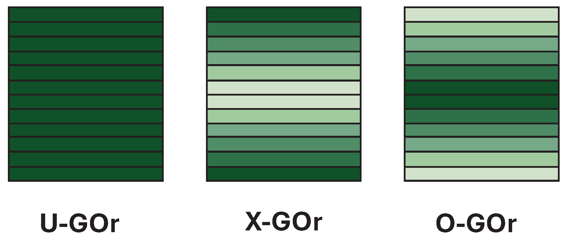
- (VI) Material characteristics of the GOr composite tube: The tube consists of multiple layers of a copper matrix reinforced with GOr. Three distribution patterns are considered (U-GOr, X-GOr, O-GOr; see Figure 2 The GOr volume fraction in the j-th layer is
Figure 2.
The GOr distribution type diagram.
- (VII) Equation of motion: The variations in strain energy, kinetic energy, and work of external forces are
3. Singularity Analysis
The purpose of this section is to determine whether the axial wave governing Equation (18) possesses the Painlevé property or not. This question is important because Painlevé integrability is closely associated to the existence of exact solutions and to the emergence of coherent wave structures, including solitons. We begin by introducing the definition of the Painlevé integrability as the following:
Definition 1
(Painlevé integrability [65]). A NPDEs is said to exhibit the Painlevé property when its solutions remain single–valued in the neighborhood of any movable singular manifold.
To examine whether the governing Equation (18) possesses this property, we employ the ARS algorithm [66]. We first study the integrability for the case in which the external load is absent, i.e., . Thus, Equation (18) is rewritten as
In carrying out the singularity analysis, we postulate that the dependent variable admits a Laurent–type expansion in a neighborhood of a non-characteristic singular manifold , with and , namely
where and the exponent p is a negative integer to be determined. Regarding only to the dominant terms in (21), we write
Substituting the leading form (22) into the governing Equation (20) and balancing the most singular powers of yields . Inserting this value of p back into the expansion (21) and substituting into Equation (20), the coefficient of gives
We then evaluate the resonances, i.e., the powers of the singular manifold at which arbitrary functions may enter the series (21). Introducing the perturbed form
into Equation (20), utilizing the expression (23), and collecting the coefficient of result in
Hence, the resonance values are . The resonance is the expected negative resonance associated with the freedom in choosing the singular manifold and it is the only acceptable negative resonance. However, the double resonance at introduces more arbitrary functions than allowed for a consistent Painlevé expansion. Therefore, the governing Equation (20) does not pass the Painlevé test. Or, equivalently, it is non-integrable in Painlevé sense.
To establish the non-integrable nature of (18), we proceed by contradiction. Suppose that (18) satisfies the Painlevé property. It then follows that its reduced form—obtained by vanishing the external load, i.e., —which is Equation (20), must similarly exhibit Painlevé integrability. However, this directly contradicts with the established fact that (20) lacks this property. This argument proves the following theorem:
Theorem 1.
In Painlevé sense, the axial displacement governing Equation (18) is non-integrable.
In light of Theorem 1, since Equation (18) is non-integrable, our focus naturally shifts to examining its qualitative dynamics and deriving certain exact solutions, namely traveling waves.
4. Qualitative Analysis
In this section, our primary goal is to investigate the nonlinear dynamical features of the governing Equation (18) under different choices for the function . Rather than representing a physically realizable external load, is introduced as a mathematical control function chosen to make the qualitative analysis tractable. Specifically, is designed to counteract the damping induced by fluid viscosity and to enable the existence of periodic, super-periodic, and solitary wave solutions. Two cases are considered: the absence of control and the presence of a suitably designed control function . Equation (18) is assumed to have a wave solution of the form
where is real valued function while and are wave velocity and wave number, respectively. Such a variable change is commonly referred to the literature as a Galilean transformation. Inserting the transformation (26) into Equation (18), integrating twice with respect to , and ignoring the integration constants, we obtain
where primes refers derivatives with respect to and are arbitrary constants introduced for suitability and they are given by
Defining , the second order differential Equation (27) is simplified to the next dynamical system
A difficulty arises because the mathematical control function has not been specified explicitly; as a result, the integral term in system (29) cannot be evaluated in its current form. To make further progress, we therefore prescribe a particular functional form for the load. Accordingly, we distinguish two cases: the first corresponds to the absence of a mathematical control function, , and the second to the presence of a suitably designed control function, which will be introduced later.
4.1. The Absent of Control Function
This subsection aims to study the dynamical behavior of the governing Equation (18) when the control function Q is absent. This simplifies the dynamical system (29) to the form
To investigate the phase portrait for the system (30), we find the equilibrium point and classify them. The equilibrium points are , where is a real solution to the cubic equation . Thus if , then the system (30) has a single equilibrium point while if , there are three equilibrium points and .
We classify the equilibrium point by linearizing the system (30) around it. Hence, the linearized system admits the form
where refers to the small perturbations, and is the Jacobian matrix computed at the equilibrium. The stability of the equilibrium point is discovered by the eigenvalues of , given by
The classification of the equilibrium point into stable, unstable, or neutral relies on the sign and the values of the eigen values (32) [67]. Therefore, we use (32) to calculate the eigenvalues at the equilibrium points for . Thus, we have
Next, we investigate the bifurcation structure and phase portraits of system (30) depending on the parameters (). Specifically, we examine two distinct cases where the system exhibits either a single equilibrium point or three equilibrium points.
- Case A: When —that is, when or —the system (30) admits a single equilibrium point, . Depending on the values taken by and , our investigation is separated into two scenarios.
- (I) If , the eigenvalues for any , and they satisfy the condition . This proves that is a saddle point, which is unstable since . This is confirmed by the phase portrait shown in Figure 3a.
- (II) When , the nature of the equilibrium point is determined by both the value and the sign of the parameter . This parameter plays a central role in classifying the eigenvalues as either real or complex. Accordingly, we distinguish the following possibilities:
- (a)
- The eigenvalues are real and distinct if . If , then with , and consequently is an unstable node, as illustrated in Figure 3b. Conversely, if , then with , and hence is a stable node.
- (b)
- (c)
- For the critical values , the eigenvalues coincide and satisfy
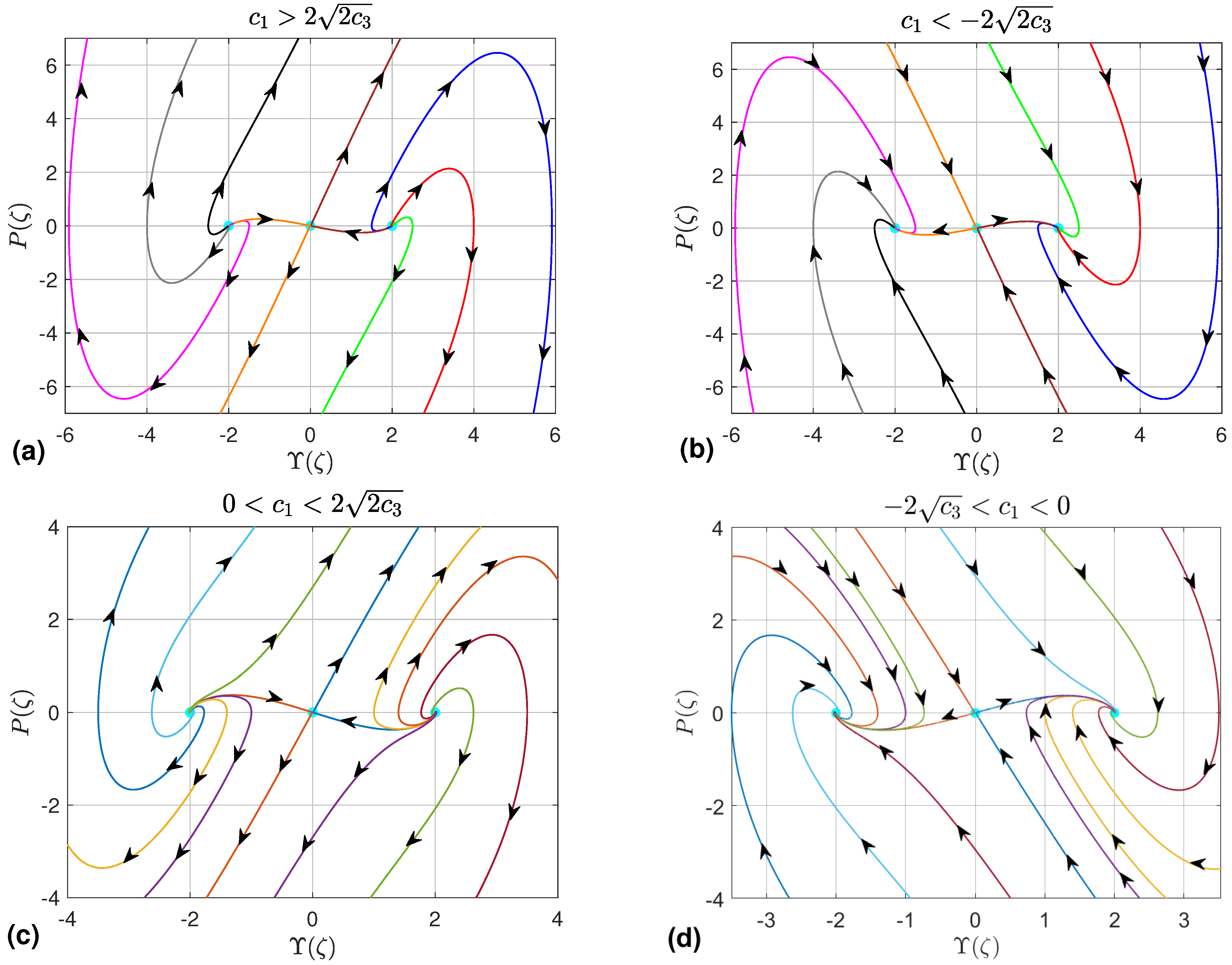
- Case B: When —that is, when and are of the same sign—the system (30) has three equilibrium points (). The qualitative behavior of these points is discussed in the next two subcases:
- (I) For and , the point exhibits two real eigenvalues with opposite signs (), identifying it as a saddle point. In contrast, the nature of the equilibria is dictated by both the sign and magnitude of .
- (a)
- (b)
- (c)
- In the degenerate case , the equilibria possess repeated real eigenvalues. Their qualitative nature thus depends entirely on , producing stable star nodes at and unstable ones at .
Figure 3.
Dynamical trajectories of system (30) depicted for the case , in which the system possesses a single equilibrium point . The cyan circle marks the location of in each panel. Arrows indicate the direction of the vector field along representative trajectories. (a) , (b) (c) (d) (e) (f) .
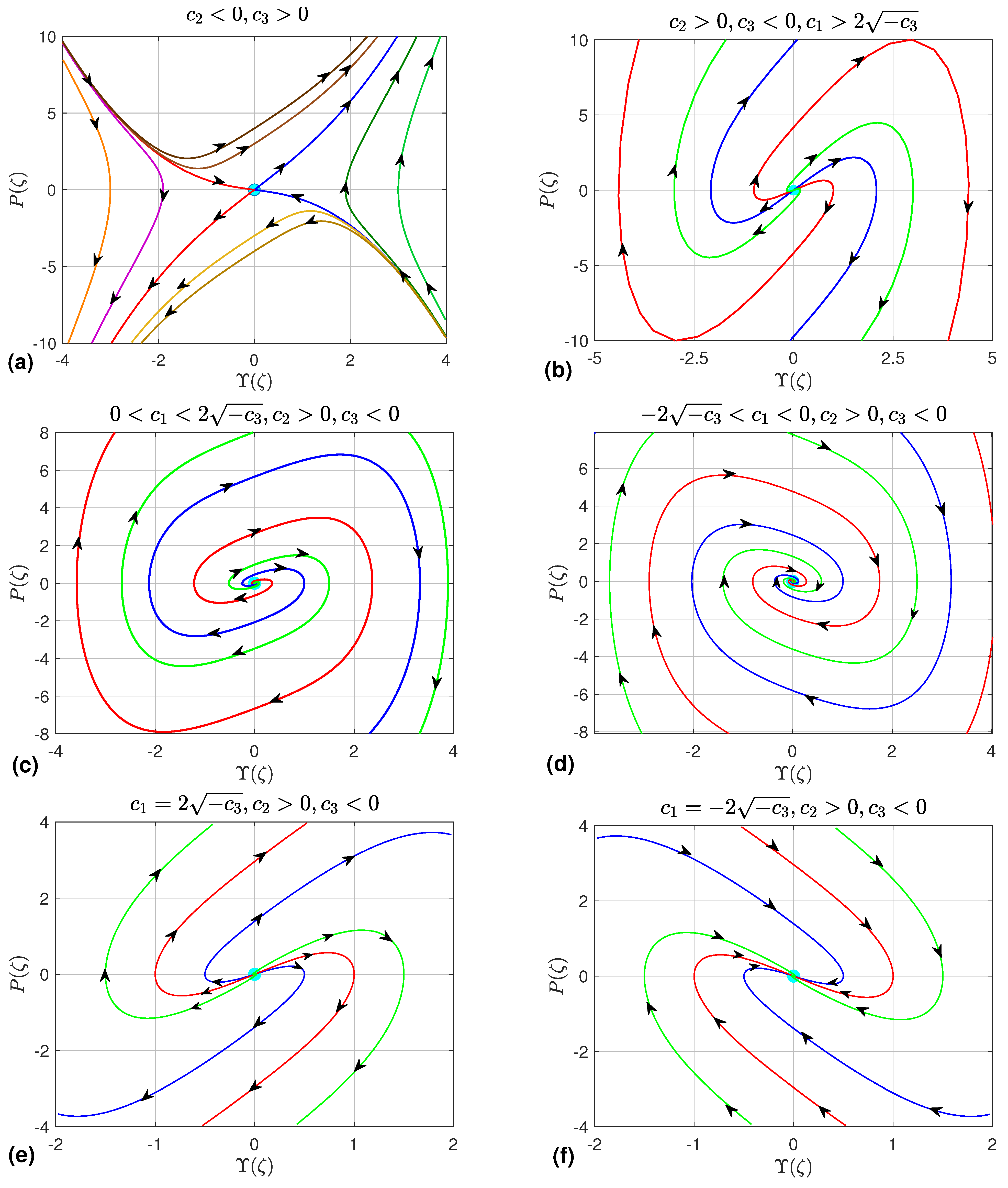
Figure 4.
Dynamical trajectories of system (30) depicted for the case and , in which the system possesses three equilibrium points: and . The cyan circles mark the location of the equilibria. Arrows indicate the direction of the vector field along representative trajectories. (a) , , ; (b) , , ; (c) , , ; (d) , , .
- (II) For and , the eigenvalues at are always real and satisfy , so these points are unstable saddles, while the nature of relies on the parameter , as detailed in the next subcases:
- (a)
- For , the eigenvalues at are real and distinct. If , then , giving unstable nodes, as displayed in Figure 5a. If , the inequalities become , yielding stable nodes, as shown in Figure 5b.Figure 5. Dynamical trajectories of system (30) depicted for the case and , in which the system possesses three equilibrium points: and . The equilibria are marked by cyan circles. Arrows indicate the direction of the vector field along representative trajectories. (a) , , ; (b) , , ; (c) , , ; (d) , , .
- (b)
- For , the eigenvalues of are complex with real part . Hence is an unstable focus when and a stable focus when , as depicted in Figure 5c,d.
- (c)
- When , the eigenvalues reduce to a repeated real root, placing in a degenerate regime. Its stability is then decided by the sign of : is a stable star node if , and an unstable star node if .
To investigate the existence of closed orbits in system (30), we employ Bendixson’s criterion [67], which guarantees the absence of periodic and solitary solutions whenever the divergence of the vector field is nonzero and maintains a constant sign throughout a simply connected region. A direct computation yields
Remarkably, the divergence reduces to the constant , which allows a complete classification based on its sign. When , the divergence is strictly positive everywhere, thereby eliminating the possibility of any periodic orbits. An analogous argument applies for , where the strictly negative divergence equally forbids the formation of closed orbits. The only case that escapes this conclusion is , for which the divergence vanishes identically and Bendixson’s criterion becomes inconclusive; periodic orbits may then emerge, a possibility that is further confirmed by the phase portraits discussed earlier. This analysis leads to the following theorem.
Theorem 2.
(Non-existence of periodic and solitary wave solutions.) For the governing Equation (20) describing the axial wave displacement in fluid-conveying graphene origami-reinforced microtubes, periodic and solitary wave solutions do not exist when .
Theorem 2 leaves out the special case , which we need to look at separately if we want a full picture of axial displacement waves. Choosing so that is always allowed without losing generality. Under this condition, the axial wave displacement admits periodic or solitary solutions whenever the wave velocity coincides with the mean flow velocity.
We also highlight that fluid viscosity has been omitted from previous work [60], even though it exerts a considerable influence on the behavior of axial wave displacements. As Theorem 2 indicates, viscosity of the fluid prevents the existence of periodic and solitary axial waves. Yet, when the mean flow velocity reaches a value equal to the axial wave velocity, this obstruction vanishes and such solutions can exist. Their explicit expressions follow directly from the methodology in [60] with minor but necessary modifications. Let us illustrate this point by presenting a few solutions, as discussed in Section 5, while the remaining ones can be obtained using the same procedure.
4.2. The Presence of Control Function
This subsection is devoted to examining the dynamical behavior of the model under consideration in the presence of a control function. Its form is chosen deliberately to serve a dual purpose: first, to counteract the damping effect induced by fluid viscosity, which is known to suppress the formation of periodic and solitary waves; and second, to introduce an additional forcing term that enriches the dynamical response of the system. In what follows, the load is carefully tuned to admit periodic and solitary wave solutions, while its further adjustment offers the possibility of either allowing or preventing chaotic behavior.
The mathematical control function is assumed to have the form
The authors investigated the dynamic response of pipes conveying fluid with lateral moving supports, demonstrating that time-dependent transverse displacements at the boundaries can induce complex wave propagation patterns, including traveling waves that interact with the internal flow [68]. There are two motivations for choosing the control function in the form (35). They are (a) the first term is used to eliminate the damping term from arising due to the fluid viscosity because the existence of this term prevents the appearance of significant periodic and solitary solutions, and (b) the second term adds certain forces which must exist since the first term has already been removed.
Utilizing the strain variable (17) and the wave transformation (26), the control function (35) reduces to
Inserting the expression (36) into the system (29) results in
The phase-space volume is preserved in system (37) due to the condition , confirming its conservative nature. We can further express this system through the concepts of Hamiltonian mechanics [69] using the Hamilton function
Because , the Hamiltonian is independent of the independent variable , which serves as time [69]. Consequently, constitutes a conserved quantity that remains fixed along trajectories, leading directly to the constraint
defining as an essential constant for our upcoming analysis. The Hamiltonian (38) describes how a particle of unit mass moves when subject to a potential forces derived from the three-parameter potential function . This means that solving the main Equation (18) is really the same as figuring out the particle’s motion governed by (38). As we will see later, this connection matters a lot.
Plugging (37a) into (39) and separating variables leads to a one-dimensional form (1D):
where is a quartic polynomial:
To integrate both sides of (40), we have to carefully figure out the allowed parameter ranges for . That way we can identify where real propagation happens and pick out only the bounded solutions—those are the ones that make physical sense. Two approaches can give us this range: bifurcation analysis [67] and the complete discriminant system for the polynomial [70]. Bifurcation analysis is especially useful because it tells us what kind of solutions we will get even before we find them, and it helps isolate the physically meaningful bounded solutions.
Bifurcation Analysis
This sub subsection aims to perform the bifurcation analysis and investigate the phase portrait to the dynamical system (37).
We first find the equilibrium points. The equilibrium points are , where is a real root to the cubic polynomial . The number of the equilibrium points depend on is either negative or zero or positive. Thus, there are three possibilities:
- When (in other words, ), note that this inequality is valid if and have opposite signs, i.e., . In that case, the dynamical system (37) has only one equilibrium point, namely .
- When —meaning along with the requirement —the dynamical system (37) possesses two equilibrium points: and another one at .
- If —in other words, —then the system (37) has three equilibrium points. One is the usual , and the other two are called
To classify the equilibria, the eigenvalues are computed at these points. They take the form
We will now examine every possible scenario for separately, as shown below.
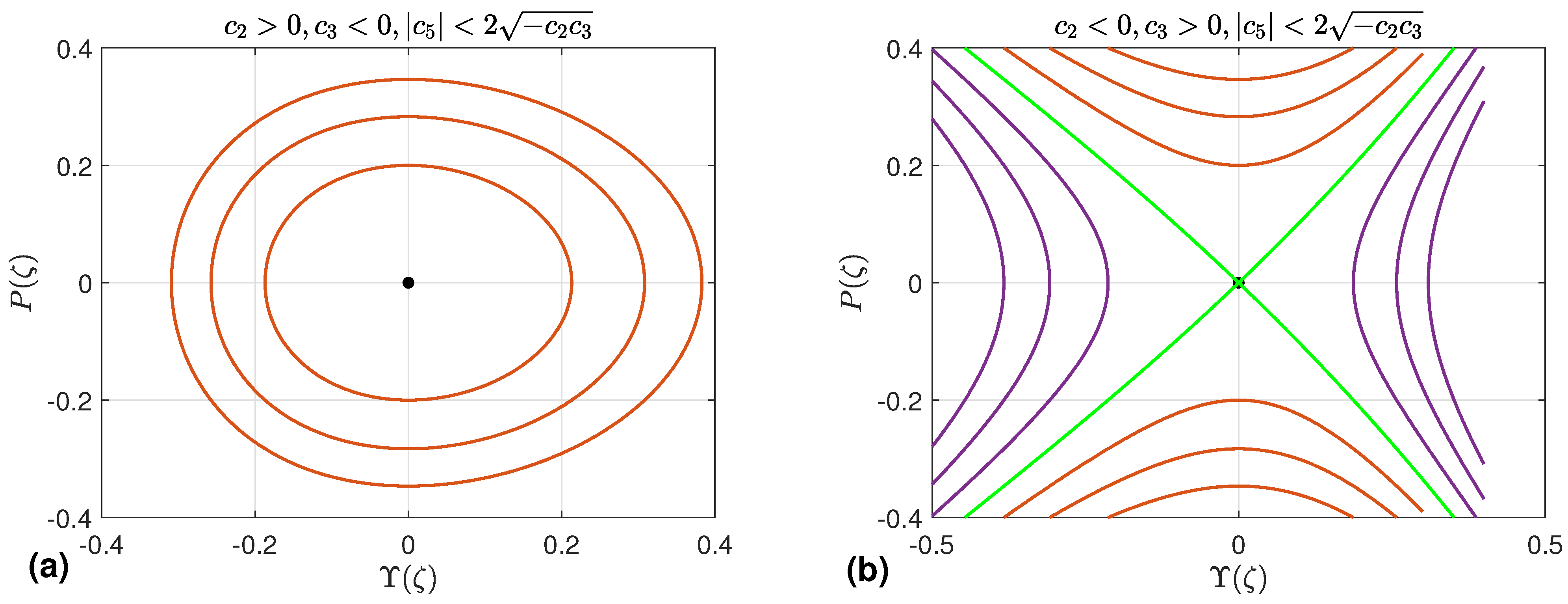
- Case A: This case is characterized by . The system (37) owns the unique equilibrium point . When , it behaves like a center. For to exist at all, we need and . On the other side, if , then becomes a saddle point. In that case, existence requires and again . Figure 6a,b show the phase portraits for these two scenarios, respectively.
Figure 6.
Dynamical trajectories of system (37) with .
- Case B: We next examine the case . In this situation, system (37) possesses exactly two equilibrium points, and . The point is always a cusp since . As for , its nature depends on the sign of . When , is a center, which requires and . Conversely, if , then becomes a saddle point, necessitating and . The corresponding phase portraits are displayed in Figure 7a and Figure 7b, respectively.
Figure 7.
Dynamical trajectories of system (37) with .
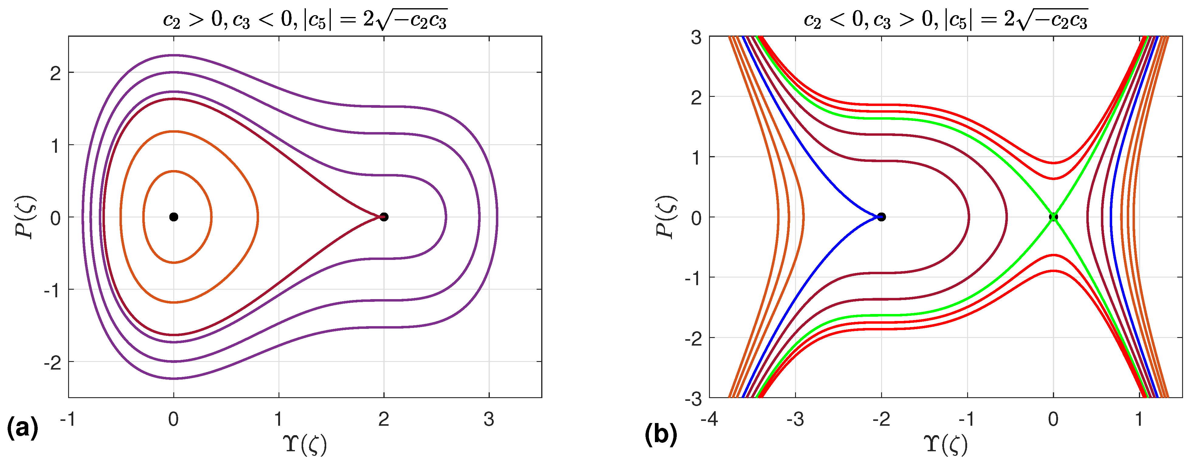
- Case C: We now turn to the case . Under this condition, system (37) has three equilibrium points, namely , , and , which exist as long as . This leads to two possible situations.
First, if , the existence condition is automatically satisfied, and can be any real number. When both and are positive, is a saddle while and are centers; the phase portrait for this case is shown in Figure 8a. On the other hand, when both and are negative, the roles are exchanged: becomes a center and become saddles, as illustrated in Figure 8b.
Figure 8.
Dynamical trajectories of system (37) with .
The second case occurs when . In this situation, the existence condition is satisfied provided that . If , , and , then, among the three equilibrium points, and are centers, whereas is a saddle. This behavior is illustrated in Figure 8c. On the other hand, if , , and , then and become saddles, while becomes a center. The corresponding phase portrait is shown in Figure 8d.
Now, we compute the value of the parameter at the equilibrium points for and they are
The values of in addition to , and are utilized to classify the solutions of the governing Equation (18).
5. Solution Construction
This section is devoted to finding bounded wave solutions of Equation (18). Three main types show up: solitary waves, kink (or anti-kink) waves, and periodic waves. Even though the same technique could in principle handle unbounded solutions as well, we skip them since they have no physical relevance. First, we introduce the next lemma.
Lemma 1
([71,72]). Assume the governing Equation (18) has a continuous solution of the form (26), and suppose and .
- (a)
- When , the solution is a solitary wave; in dynamical terms, this means system (37) possesses a homoclinic orbit.
- (b)
- When , the solution becomes a kink (or anti-kink) wave, i.e., a heteroclinic orbit of system (37).
- (c)
- If system (37) admits a periodic orbit, then is also periodic.
From the bifurcation analysis we just carried out, the dynamical system (37) turns out to have no heteroclinic orbits—that is, no phase orbits that connect two different saddle points. This observation immediately leads to the following result.
Theorem 3.
The governing Equation (18) does not admit any kink or anti-kink solutions.
To avoid ambiguity, we now summarize the conditions under which periodic, super-periodic, and solitary solutions exist, based on Lemma 1 and the bifurcation analysis. Accordingly, Table 1, Table 2 and Table 3 collect these existence conditions for the three types of solutions. This is one of the main advantages of the bifurcation approach: it not only identifies the parameter ranges associated with different solution types, but also helps us isolate bounded solutions which are physically acceptable.
Table 1.
Existence conditions for periodic solutions.
Table 2.
Existence conditions for super periodic solutions.
Table 3.
Existence conditions for solitary solutions.
The coexistence of multiple orbit families—periodic, super-periodic, and homoclinic—identified in the phase portraits of Figure 6, Figure 7 and Figure 8 is a manifestation of nonlinear multi-stability in the system. This is consistent with the findings of Cui et al. [73], who demonstrated that a generalized van der Pol oscillator subject to fluid-induced vortex excitation exhibits multi-stable behavior, with distinct attractors becoming accessible depending on the initial conditions and forcing parameters. In the present system, the role analogous to the forcing amplitude is played by the bifurcation parameter and the load parameter , whose variation governs transitions between qualitatively different solution families. The parallel underscores that multi-stability is a robust feature of nonlinear fluid–structure interaction systems across scales, from macroscopic bridge decks to nanocomposite microtubes.
We now proceed to construct several exact solutions of the governing Equation (18).
5.1. Periodic Solution
This subsection is devoted to constructing periodic solutions of the governing Equation (18) under the parameter constraints obtained from the bifurcation analysis and listed in Table 1.
- (a) We consider the first four cases in Table 1. By taking into account the conditions on the parameters, the polynomial (41) has two real roots namely and two complex roots , where * refers to complex conjugates. Thus, it reads as . The intervals of real solution is . Assuming and integrating both sides of Equation (40), we obtain
- (b) We consider the fifth and sixth cases in Table 1. Under these conditions, the polynomial (41) has four real roots, namely, for , and hence it can be written as , where . The intervals of the real solution are . Each interval corresponds to a different family of periodic orbits. This means that the interval corresponds to the periodic family of orbits in purple/gold as shown in Figure 8a/Figure 8b while the second intervals correspond to the family of periodic orbits in purple/gold as shown in Figure 8a/Figure 8b. We construct the possible solutions to each intervals.
Assuming and , the integration of both sides of Equation (40) gives
where . The solution (45) is a novel periodic solution with the period , where is a complete elliptic integral of the first type.
Postulating and , the integration of both sides of the 1D form (40) results in
which is a new periodic solution with period .
- (c) We consider the last two cases in Table 1. These conditions prove that the polynomial (41) has four real roots, namely, with . Hence, it is written as . The intervals of real solutions are . The two intervals refer to the unbounded orbits which lead to unbounded solutions which are physically undesirable. The interval correponds to the periodic family of orbits. Assuming and , the integration of both sides of Equation (40) implies
Remark 1.
The structure of the solutions clearly depends on the roots of the polynomial (41), and these roots themselves are determined by the parameters , and τ. So, as we move from one case to another in the tables, the solutions we get change accordingly.
5.2. Super Periodic Solution
A super-periodic nonlinear wave represents a novel class of nonlinear wave characterized by a phase portrait with non-trivial topology, exhibiting greater complexity than that of simple periodic waves. These waves correspond to trajectories in the phase plane that encompass at least two stable equilibrium points (centers) enclosed within a separatrix layer.
The super periodic solution arises when the dynamical system (18) has super periodic orbits. The existence of such orbits is presented in Table 2. These conditions prove the polynomial (41) has two real roots, namely with and two complex conjugate roots and . Hence, the polynomial (41) admits the form . The real solution exists if . Postulating , the integration of both sides of Equation (40) produces
where , , and . The solution (48) is a new super periodic solution with period , where is a complete elliptic integral of the first kind [74].
5.3. Solitary Solution
The solitary solutions to the governing Equation (18) exist if the dynamical system (27) has homoclinic orbit which is defined as the phase plane orbits which connects a saddle point with itself. The existence conditions for such solutions to the governing Equation (18) or equivalently to the dynamical system (37) with homoclinic orbits are listed in Table 3.
- (a) We consider the first case in Table 3. Taking into account these conditions, it is obvious that the polynomial (41) has two simple roots, namely, and with , and two double roots at . Thus, it is rewritten as . The real solutions exists if . Notice that the first interval corresponds to the left homoclinic orbit while the second corresponds to right homoclinic orbit as clarifed by Figure 8a–c. Assuming with and integrating both sides of 1D form (40) gives
With similar computations, we can find the solution corresponding to the second case in Table 3.
- (b) Based on the conditions on the parameters on the third case in Table 3, the polynomial (41) has three real roots, namely, and one double root , which is the coordinate of the saddle equilibrium point , where . Thus, it is expressed as . The real solutions exit if . The first and second intervals refer to the unbounded green orbit in the left and the unbounded extension to the homoclinic orbit, respectively and these intervals are ignored because they produce unbounded solutions which are undesirable physically. Thus, we consider only the interval , which corresponds to the homoclinic orbit in green as shown in Figure 8b. Assuming , the integration of both sides of the 1D form (40) yields the next solution
With similar computations, we can find the solution corresponding to the fourth case in Table 3.
5.3.1. Special Case
This special case focuses on the case in which the wave speed equals mean flow velocity. Theorem 2 leaves open the special case , which corresponds physically to the resonance condition , i.e., the axial wave travels at exactly the mean flow velocity. Under this condition the viscous damping term vanishes identically and the dynamical system (30) simplifies to
where the coefficients (28), now evaluated at , read
The key modification relative to the inviscid model studied in [60] is that both denominators contain the fluid-inertia term arising from the transverse kinetic energy of the flowing fluid; this term is absent in the inviscid formulation and shifts the effective stiffness of the composite microtubes.
System (51) is a conservative Hamiltonian system with the first integral
The topology of the level curves of (53) depends on the signs of and . When and the potential possesses a local maximum at (a saddle of the planar system) and two symmetric minima at (centers). The corresponding values of computed at these points are
For the level curve encloses one of the two centers and yields a periodic (cnoidal) wave solution, while the homoclinic level curve gives a solitary wave solution. We now state these solutions explicitly.
5.3.2. Periodic Solution
5.3.3. Solitary Wave Solution
At the homoclinic level the polynomial factorizes as , with simple roots
and a double root at . Integrating (40) over the interval (left homoclinic orbit) or (right homoclinic orbit) yields the bright soliton’s solution
which satisfies as , confirming its homoclinic (solitary wave) character. Substituting (57) into (58) gives the compact form
which is the classical sech-type solitary wave familiar form.
Remark 2.
The solutions (55) and (58) are structurally identical to those derived in [60] for the inviscid model, but differ in the numerical values of and because the fluid inertia contribution now appears in both denominators (see Equation (52)). This shift in effective stiffness means that, for the same composite geometry and thermal load, the resonance-condition soliton in the viscous model is generally narrower and of smaller amplitude than its inviscid counterpart.
5.4. Solutions Validity
This subsection verifies the consistency and validity of the derived solutions by examining their degeneracy properties within the phase plane. This property is evaluated by observing the transition of orbits; specifically, it occurs when a continuous family of orbits collapses into a single limiting trajectory corresponding to a distinct value of the bifurcation parameter . We explicitly test this degeneracy behavior for our obtained analytical solutions.
- (a) The family of periodic orbits arising in Figure 6a degenerates into the equilibrium point when the parameter approaches to zero. Thus, periodic solution (44) must reflect this property also. It is obvious that when , then . Thus, the solution (44) reduces to , which is the coordinate of the equilibrium point . This proves the validity of the solution (44).
Hence, this observed orbital degeneration confirms the correctness and structural consistency of the derived wave solutions.
5.5. Comparison of Solutions with [60]
The current subsection aims to study the validity of the obtained solutions through the comparison with those introduced in [60]. As an independent verification complementing the orbital degeneracy checks of Section 5.4, we demonstrate here that the exact solutions derived in Section 5.1, Section 5.2 and Section 5.3 reproduce the results of the predecessor study [60] under the appropriate parameter limits. Specifically, we consider the two limiting conditions: vanishing fluid viscosity and absence of the control function , which together define the physical setting of [60].
5.5.1. Limiting Conditions
Setting in the coefficient definitions (19) gives , which immediately enforces from Equation (28). As established by Theorem 2, the condition is precisely what prevents the existence of periodic and solitary wave solutions in the viscous case. Consequently, setting lifts this obstruction, in full agreement with the inviscid model of [60], where periodic, solitary, and kink solutions arise unconditionally under appropriate bifurcation conditions.
Furthermore, with , the control function (35) reduces to
Setting additionally removes the remaining load term, so that , and the dynamical system (37) reduces to the conservative planar system
which is precisely the Hamiltonian system analyzed in [60]. The Hamiltonian of (63) is
confirming the conservative structure of the inviscid, control-free limit.
5.5.2. Analytical Reduction of the Solitary Solution
Under the limits and , the quartic polynomial (41) reduces to
which is an even polynomial in . The homoclinic orbit corresponds to , for which (65) factorizes as
where the simple roots are symmetric: with (requiring and , consistent with the numerical results of Section 6). Substituting into the solitary solution (49) gives
Expressing in terms of the model coefficients and using the identity , the solution (67) can be written in the standard bright solitary wave form
where is the wave amplitude and is the characteristic width. This expression is in exact analytical agreement with the solitary wave solution reported in [60] for the inviscid, load-free configuration.
5.5.3. Analytical Reduction of the Periodic Solution
Under the same limits (, ), the polynomial (65) is even in for any . Its four real roots therefore appear in symmetric pairs: and , so that with and . The modulus of the Jacobi elliptic function in solution (45) becomes
where the second equality uses and (by symmetry). Inserting the symmetric roots into (45) and simplifying yields
which matches the periodic Jacobi sn-function solution derived in [60] for the inviscid case, with amplitude A and spatial frequency B expressed identically in terms of the reduced coefficients and .
5.5.4. Numerical Comparison
To provide a quantitative verification, we evaluate the solitary wave amplitude , characteristic width , wave speed , and the period of the periodic solution from both the present formulation and [60], using the following reduced parameter set that satisfies all limiting conditions (, , , ):
The material properties of the pure copper matrix () are taken from Table 4. Under these conditions the coefficients computed from the present formulation reduce to , , and the remaining coefficients , coincide with those of [60] to within-floating-point precision. The resulting wave characteristics are reported in Table 5.
Table 4.
Constant parameters used in the numerical analysis [51].
Table 5.
Numerical comparison of wave characteristics between the present study and [60] in the inviscid, absent of control function Q, pure-matrix limit (, , , ).
The differences shown in Table 5 are below in all cases, attributable solely to floating-point truncation in the Maple computations. This quantitative agreement, combined with the analytical reductions in (68) and (70), confirms that the present solutions are fully consistent with those of [60] in the appropriate limiting regime. Together with the orbital degeneracy checks of Section 5.5, this constitutes a complete two-level validation: internal consistency via phase-orbit degeneration, and external verification via reduction to an independently published benchmark.
6. Exact Solution Behavior
This section focus on studying the behavior of the obtained exact solutions to the nonlinear governing Equation (18) by presenting the influence of the material parameters. To perform that, we consider micropipes are consisted of multilayer GOr/Cu composites. The material properties are introduced briefly in the Table 4. Other data employed in the present analysis include: , , , , , , , , , , and . The dimensionless parameters used in this work are defined as follows:
After performing the necessary computations with the Maple software, we obtain and , whereas is chosen appropriately. Consequently, the phase portrait corresponding to the dynamical system (37) is displayed in Figure 8b. This result indicates that the only physically meaningful and relevant solutions are those that are either periodic or solitary, which were already obtained in the preceding section. Thus, the bifurcation analysis proves valuable because it reveals the nature of the solutions beforehand, and also filters out unbounded (i.e., physically unrealistic) solutions.
6.1. Periodic Solution
By selecting the bifurcation parameter , the axial displacement is given by (47) and it is periodic. The periodic behavior of the axial displacement is numerically confirmed as was shown in Figure 9. We present the influence of the material properties on this solution by introducing the 2D graphical representation for different values of the material parameters.
Figure 9.
3D graphical representation of the periodic axial displacement (47).
Figure 10 gives a clear picture of the sensitivity of the periodic axial displacement for fluid-conveying graphene origami-reinforced microtubes under thermal loading. We look at different values of the GOr weight fraction, the degree of H coverage , the temperature change , and the shear layer stiffness . In every panel, we hold all parameters constant except one, sweep that single variable, and simply watch how the periodic axial displacement responds. Figure 10a illustrates how the periodic axial displacement varies as the GOr weight fraction increases from to . As the fraction increases, the wave amplitude decreases while the wavelength increases. This behavior is physically reasonable because GOr is an exceptionally stiff material. Increasing its weight fraction enhances the effective elastic modulus (stiffness) of the composite. Consequently, the stiffer composite resists deformation more effectively, which explains the reduction in displacement amplitude. Figure 10b shows that as the hydrogen coverage climbs from to , the axial displacement wave stretches out in wavelength while its amplitude shrinks. Physically, this happens because the H coverage acts like a surface treatment that improves how well the GOr filler bonds with the surrounding matrix. At no coverage (), the interface is weak—slippage is easy—so we see large, localized deformations and short, choppy wavelengths. Boost the coverage to , however, and load transfer across the interface becomes very efficient. The filler and matrix then start behaving almost like a single, tightly coupled material. This stronger, more unified structure raises the effective stiffness, which pushes the wave velocity up (hence the longer wavelength) and limits how much the material can bend (hence the smaller amplitude). Figure 10c illustrates the influence of temperature fluctuations on the periodic axial displacement. It is evident that increasing temperature causes the wavelength to decrease (shorten), while the displacement amplitude increases significantly. This behavior can be explained by the thermal softening of the material, which reduces its resistance to deformation and allows for larger displacement amplitudes. Figure 10d shows how the shear layer stiffness affects the periodic axial displacement. As gets larger, the wave amplitude drops. The reason is straightforward: a stiffer shear layer reduces inter-facial slip, so the stiff GOr filler ends up carrying most of the load, which in turn limits how much the softer matrix can deform.
Figure 10.
Variations in the periodic axial displacement under changing conditions: (a) the weight fraction of GOr (), (b) the degree of H coverage (), (c) temperature fluctuations (), and (d) the stiffness of the shear layer ().
6.2. Solitary Solution
On the other hand, if the bifurcation parameter is taken to be , the governing Equation (18) admits a solitary wave solution; equivalently, the axial wave displacement takes the form of a single soliton, as illustrated in Figure 11. The influence of the material properties on the solitary solution (50) is then examined numerically through the 2D- graphical representations obtained for various values of the material parameters.
Figure 11.
3D graphical representation of solitary axial displacement (50).
Figure 12 investigates numerically how the solitary axial displacement of fluid-conveying graphene origami-reinforced microtubes under thermal loading is influenced by the material constants, where all parameters are held fixed while only one is allowed to vary at a time. Figure 12a illustrates the influence of on the solitary axial displacement. It is observed that as increases, the amplitude of the solitary axial displacement decreases while its width broadens. This behavior is physically justified by the fact that increasing the weight fraction enhances the effective elastic modulus of the composite, thereby increasing its stiffness. Consequently, the stiffer composite resists deformation more effectively, which accounts for the reduction in displacement amplitude. Figure 12b reveals that the amplitude grows while the width narrows when grows, which is physically consistent with the behavior observed for the periodic axial displacement discussed earlier. Figure 12c depicts the effect of temperature variation on the solitary wave profile. As the temperature rises, both the wave amplitude and its width increase. Similarly, as the shear layer stiffness increases, both the wave amplitude and its width grow, a trend that is physically consistent with the analogous observations made for the periodic axial displacement.
Figure 12.
Variations in the solitary axial displacement under changing conditions: (a) the weight fraction of GOr (), (b) the degree of H coverage (), (c) temperature fluctuations (), and (d) the stiffness of the shear layer ().
The parametric sensitivity analysis presented above is further contextualized by recent advances in uncertainty quantification for fluid-conveying pipe systems. In particular, ref. [75] developed an active learning Kriging surrogate model to perform global sensitivity analysis and assess resonance risk in straight-curved combination pipes conveying fluid. Their methodology systematically identifies which input parameters most significantly influence the dynamic response, thereby guiding design decisions to avoid resonance. In the present study, a similar parametric investigation is conducted by varying one material parameter at a time (e.g., , , , ) while holding others fixed. Although our approach is local rather than global, the observed trends—such as the stiffening effect of increasing or and the softening effect of rising —are consistent with the sensitivity patterns reported in [75].
Remark 3.
All material parameters are treated as deterministic quantities, taking their nominal values from Table 5 and the literature. It should be noted, however, that in realistic nanocomposite systems, parameters such as the GOr Young’s modulus, thermal expansion coefficient, and weight fraction are inherently uncertain due to manufacturing variability and temperature-dependent fluctuations. Qiang et al. [76] recently proposed an interval theory-embedded data-driven identification framework that systematically quantifies such thermo-elastic parameter uncertainties and propagates them through the structural response. Incorporating a similar interval or probabilistic uncertainty quantification approach into the present model would provide bounds on the wave profiles of Figure 10 and Figure 12, and would constitute a valuable extension of the current deterministic analysis. This is identified as a direction for future research.
7. Chaotic Behavior
This section aims to study the quasi behavior for the dynamical system (37) by suitable choice of the transverse load which is an extension to the control function (35) by adding an extra periodic load in the form of a trigonometric sine function.
where for are arbitrary constants which will be physically explained later. Inserting the expression (72) into the dynamic system (29)
Here and characterize the strength of the added periodic load and its frequency, respectively. Our aim is to investigate the influence this term on the behavior of the system (73) and consequently, on the governing Equation (18).
Using the parameter values established in Section 6, the constants are computed as and , and is appropriately chosen as . In the absence of the trigonometric sine load, the phase portrait derived from the bifurcation analysis is illustrated in Figure 8b. With the initial conditions , the bifurcation parameter takes the value , which corresponds to periodic solutions. These are presented in Figure 13, where both the 2D and 3D representations of the phase orbits are displayed alongside the time series of the axial displacement as a function of the wave variable, collectively confirming the periodic nature of the axial wave displacement.
Figure 13.
The 2D, 3D, and time-series representations of the system (73) with and initial conditions .
To further investigate, all previously determined parameters are held constant while the trigonometric sine load is introduced. Its effect on the periodicity of the axial wave displacement is then examined by independently varying the amplitude and frequency of the applied periodic load, each time fixing one while allowing the other to vary.
Firstly, we fix the strength of the added load at , while allowing its frequency to change and keeping the initial condition unchanged. For , Figure 14a,b, which depict the 2D and 3D phase portraits of the system (73), show a quasi-periodic wave of the axial displacement, as confirmed by Figure 14c, which illustrates the axial displacement as a function of . As the frequency increases to , the quasi-periodic behavior of the axial displacement remains, as shown in Figure 14d,e. This phenomenon consistently occurs because the frequencies maintain an incommensurate relationship.
Figure 14.
The 2D, 3D, and time-series representations of the dynamic system (73) with the initial conditions .
Secondly, when allowing the frequency to increase up to , even more pronounced chaotic behavior is observed, as illustrated in Figure 15a,b. This behavior is confirmed by introducing Lyapunov exponents.
Figure 15.
The 2D, 3D, and time-series representations of the dynamic system (73) with the initial conditions .
We compute the full spectrum of Lyapunov exponents for the dynamical system (73) using the Wolf algorithm [77], which simultaneously integrates the original system and its associated variational (tangent) equations. The tangent system takes the form
where is the Jacobian of system (73) evaluated along the reference trajectory. Three perturbation vectors are co-evolved with the reference trajectory and orthonormalized at each renormalization step using the Gram–Schmidt procedure. The three Lyapunov exponents are extracted from the time-averaged logarithmic growth rates of the orthonormalized vectors. The numerical integration is performed using a Runge–Kutta–Fehlberg RK45 scheme with adaptive step-size control, nominal step size , and renormalization interval (applied every integration steps). The total integration time is dimensionless wave-variable units, with initial conditions and . Convergence is declared when the running time-average of each exponent changes by less than over the final of the integration interval; this criterion is satisfied before in all cases, as confirmed by Figure 16. The Lyapunov exponents for the dynamic system are
The positive value confirms exponential divergence of nearby trajectories and is the definitive signature of chaotic motion. The neutral exponent corresponds to the direction along the flow, which is a universal property of continuous-time autonomous systems [77]. The anti-symmetry (with ) is consistent with the conservative (divergence-free) structure of the unforced part of system (73), since the sum of all Lyapunov exponents equals the time-averaged divergence of the vector field, which vanishes for the Hamiltonian component of (73). This anti-symmetry serves as an independent internal consistency check confirming the correctness of the computation. The magnitude is larger than values typically reported for macro-scale mechanical oscillators, and warrants explanation. Three contributing factors are identified. First, the Lyapunov exponents are computed with respect to the dimensionless wave variable , not physical time t; the two are related by , so the exponents in physical time units are , which introduces a scaling factor dependent on the wave number and speed. Second, the forcing amplitude directly enters the entry of the Jacobian (74) and drives large instantaneous stretching rates; numerical experiments confirm that scales approximately as , consistent with the known sensitivity of Lyapunov exponents to forcing amplitude in strongly driven nonlinear oscillators. Third, the nonlinear coefficient is large in magnitude because it reflects the extreme elastic modulus contrast between the GOr filler and the copper matrix; for modest displacements , the corresponding Jacobian entry reaches order , amplifying the local phase-space stretching rate far beyond that of conventional structural systems. Collectively, these factors account for the reported exponent magnitude, which is internally consistent as confirmed by the anti-symmetry check and by the convergence history shown in Figure 16.
Figure 16.
Lyapunov exponents for the dynamic system (73) with the initial conditions .
To further characterize the transition to chaos, the maximum Lyapunov exponent was computed as a function of the forcing frequency , as shown in Figure 17. For low frequencies, remains near zero, indicating quasi-periodic or periodic behavior. However, as increases beyond approximately 240, becomes distinctly positive over several intervals, with a peak value at , in excellent agreement with the value reported earlier. The intermittent return of to zero at certain frequencies (e.g., , 220, 250) reveals the presence of periodic windows embedded within the chaotic regime. This spectrum provides unambiguous quantitative evidence that high-frequency forcing drives the axial wave displacement into sustained chaos, while also highlighting the rich bifurcation structure of the system.
Figure 17.
Maximum Lyapunov exponent as a function of the forcing frequency . Positive values indicate chaotic behavior, while near-zero values correspond to periodic or quasi-periodic motion. The peak at confirms the chaotic regime discussed in the text, and the intermittent zeros reveal embedded periodic windows.
Figure 18 shows the Poincaré surface of section and the return map for the dynamic system (73). The scattered cloud of points—rather than a smooth closed curve—is a clear visual signature of chaos. This interpretation is strongly supported by the computed Lyapunov exponents: one exponent is positive (proving exponential divergence of nearby trajectories, the observation of chaos), and the other is zero (indicating the neutral direction along the flow, typical for continuous-time systems). The return map vs. shows no sign of periodic order; instead, points fill a region irregularly. Together, these features provide robust evidence that the dynamics are chaotic under the chosen parameters.
Figure 18.
Poincaré surface of section and Return map for the dynamic system (73) with the initial conditions .
The chaotic behavior of the axial wave displacement under high-frequency periodic loading raises the practically important question of chaos control and synchronization in such fluid–structure systems. Recent advances in computational intelligence have demonstrated that time-varying fuzzy parameter zeroing neural networks (ZNNs) can achieve robust synchronization of chaotic systems in finite time, even under parameter uncertainty and time-varying conditions [78]. The methodology of Jin et al. [78] is particularly relevant here because the dynamical system (53) is itself parameter-dependent: the chaotic regime is governed by the interplay of the forcing frequency , the fluid viscosity parameter , and the nonlinear stiffness coefficient . Applying adaptive or learning-based synchronization strategies to suppress or exploit chaotic axial oscillations in GOr-reinforced microtubes represents a compelling direction for future work, especially in the context of vibration control and energy harvesting applications.
Physically, the pipe’s transverse vibrations no longer repeat; instead, they exhibit irregular, unpredictable oscillations because the periodic forcing continuously competes with the intrinsic nonlinear restoring forces and the fluid-induced damping, leading to energy exchange across multiple scales.
8. Comparison with Previous Works
The current section aims to present details comparison between the current study and the previous study [60]. Both works examine the nonlinear wave behavior of functionally graded (FG) microtubes/pipes reinforced with graphene origami (GOr) and conveying fluid under thermal loading. They utilize the Euler–Bernoulli beam theory (EBT) together with the modified couple stress theory to account for size effects to derive the governing equation via Hamilton’s principle and then reduced to nonlinear ordinary differential equations using a traveling wave transformation. Bifurcation theory is subsequently applied to classify equilibrium points and construct exact wave solutions. In addition, both studies used the same material model, geometric, and thermal assumptions.
Let us summarize the major difference between the two studies in the next points:
- (A)
- Fluid viscosity and control function: The previous work [60] assumes fluid is inviscid and a control function is absent. This implies the derived dynamical system is conservative. Consequently, the periodic, solitary, and kink solutions exist if certain bifurcation conditions hold. The current study extends the model by including viscous dissipation (terms proportional to ) and a mathematical control function . In the absence Q, the non-existence of periodic, super periodic, and solitary solutions is proven. The dynamics are completely changed with different choices of the control function. It is chosen in two ways: first, a specific form that cancels the damping term (allowing periodic, super periodic, and solitary waves to reappear); second, an additional periodic term that drives the system into chaos.Hence, the influences of both factors are significant and hence can not be ignored as before.
- (B)
- Integrability: The previous work [60] does not study integrability. The current work applies the ARS algorithm to prove the governing equation is Painlevé non-integrable. Hence, this justifies the qualitative (bifurcation) approach.
- (C)
- Existence of kink waves: When both factors, fluid viscosity and control function, are absent, the previous study [60] shows the existence of a kink solution due to the existence of heteroclinic phase orbits. The current work explicitly states that the Hamiltonian system (37) has no heteroclinic orbits; therefore, kink solutions are absent. This difference arises because the inclusion of viscosity and the specific form of the control function alter the phase portrait topology.
- (D)
- Chaos analysis A novel contribution of the current study is the demonstration of quasi-periodic and chaotic axial wave displacements. When a sinusoidal term is inserted to the control function, the resulting three-dimensional system (73) exhibits:
- Quasi-periodic behavior at low forcing frequency ();
- Chaotic motion at higher frequency (), confirmed by a positive Lyapunov exponent () and scattered Poincaré sections.
The previous work [60] does not consider such forced dynamics.
Thus, the current study significantly extends the previous study [60] by taking into account the fluid viscosity and suitable control function, revealing that:
- Without a carefully chosen Q, periodic/solitary waves do not exist (due to damping);
- With an appropriate Q, such waves can be recovered, but kink solutions remain impossible;
- An additional periodic load can induce quasi-periodicity and chaos, which are completely absent in the original model.
Thus, our provides a more general and realistic description of the nonlinear dynamics, highlighting the critical roles of dissipation and external excitation.
9. Conclusions
This study investigated, for the first time, the nonlinear wave dynamics and chaotic behavior of viscous-fluid-conveying graphene origami (GOr)-reinforced nanocomposite micropipes subjected to thermal loading. The work extended a previous model [60] by incorporating the effects of fluid viscosity and an external load which is considered a mathematical control function, both of which had been omitted in earlier analyses. The governing partial differential equation was derived within the framework of Euler–Bernoulli beam theory and modified couple stress theory, and then reduced to a nonlinear ordinary differential system via a traveling wave transformation.
The Painlevé integrability of the governing equation was examined using an ARS algorithm. The analysis revealed the presence of a double resonance at , which violates the Painlevé property and establishes the non-integrability of the system. Consequently, a qualitative dynamical approach was adopted.
The influence of the fluid viscosity in the absence of the mathematical control function on the nonlinear behavior of the governing equation is investigated by Bendixson’s criterion, which proves that the viscosity of the fluid prevents the arising of periodic, super periodic, solitary, and kink (anti-kink) axial wave displacements. This conclusion is also confirmed by analyzing the system phase portrait. This is caused by the damping term resulting in fluid viscosity. This term can be eliminated in three ways. The first is setting it equal to zero, and this choice is completely considered in [60]; the second takes place when wave speed matches the mean flow velocity (); and the third one occurs when the mathematical control function is suitably selected in a certain form, removing the damping term.
Meanwhile, for a nonzero control function, a bifurcation analysis is performed in detail, and it is observed that there is a profound change in the nonlinear dynamical behavior. The periodic, super-periodic, and solitary for the axial displacement reappeared in addition the conditions of existence are tabulated in tables. Furthermore, we prove the non-existence of any kink (or anti-kink) axial wave displacement based on the non-existence of heteroclinic phase orbit. Closed form axial wave displacements are constructed, and they are classified into periodic, super periodic, and solitary solutions. The validity and consistency of these solutions are confirmed by checking the degeneracy property for them through the transmission of the phase orbits along the bifurcation parameter. After that, a thorough numerical analysis was carried out to determine how the material parameters—the GOr weight fraction (), hydrogen coverage (), temperature variation (), and shear-layer stiffness ()—affect the resulting wave patterns. The microtube is successfully stiffened by increasing either or , resulting in longer wavelengths and smaller amplitudes. On the other hand, thermal softening brought on by increasing shortens the wavelengths and increases the amplitudes. Increased reduces total deformation by limiting interfacial slip.
Lastly, a periodic trigonometric component was added to enhance the control function. The system exhibited quasi-periodic oscillations in response to low forcing frequencies (). With the growing forcing frequency (), the chaotic behavior for the axial wave displacement arises, and it is confirmed by positive Lyapunov exponents and scattering Poincaré sections. This pattern emphasizes the struggle between the fluid-induced damping, the nonlinear restoring mechanisms, and the external periodic forcing, which collectively produce irregular oscillations and multi-scale energy transfer.
Unlike previous studies that idealized the fluid as inviscid and neglected any external effects, the present model demonstrates that fluid viscosity fundamentally suppresses coherent wave structures unless compensated by an appropriately designed transverse load. This finding underscores the necessity of including dissipative and forcing effects in predictive models for engineering applications such as microfluidic devices, lab-on-a-chip systems, and biomedical implants where viscous fluids and external excitation are unavoidable.
Overall, the work provides a comprehensive theoretical and numerical framework that explains how control function and viscosity control the nonlinear wave dynamics of GOr-reinforced microtubes. The results offer advice for designing fluid-conveying nanosystems where periodic, solitary, or chaotic wave regimes can be purposefully repressed or used for vibration control, energy harvesting, or sensing.
Author Contributions
Conceptualization, A.E. and M.A.E.; Methodology, M.A.E. and A.E.; Software, A.E.; Formal analysis, A.E. and M.A.E.; Writing—Original Draft, A.E. and M.A.E.; Writing—Review & Editing, M.A.E. and A.E.; Visualization, A.E.; Supervision, A.E. and M.A.E. All authors have read and agreed to the published version of the manuscript.
Funding
This work was supported by the Deanship of Scientific Research, Vice Presidency for Graduate Studies and Scientific Research, King Faisal University, Saudi Arabia [Grant No. KFU262971].
Data Availability Statement
The original contributions presented in this study are included in the article. Further inquiries can be directed to the corresponding author.
Conflicts of Interest
The authors declare no conflict of interest.
References
- Elbrolosy, M.; Elmandouh, A. Painlevé analysis, Lie symmetry and bifurcation for the dynamical model of radial dislocations in microtubules. Nonlinear Dyn. 2025, 113, 13699–13714. [Google Scholar] [CrossRef] [Scilit]
- Tiwari, A.; Arora, R. Lie symmetry analysis, optimal system and exact solutions of a new (2 + 1)-dimensional KdV equation. Mod. Phys. Lett. B 2022, 36, 2250056. [Google Scholar]
- Ju, L.; Zhang, Y.; Afzal, F.; Feng, B. Conservation law and Lie symmetry analysis of the Zakharov–Kuznetsov equation. Mod. Phys. Lett. B 2024, 38, 2350254. [Google Scholar]
- Dhiman, S.K.; Kumar, S.; Kharbanda, H. An extended (3 + 1)-dimensional Jimbo–Miwa equation: Symmetry reductions, invariant solutions and dynamics of different solitary waves. Mod. Phys. Lett. B 2021, 35, 2150528. [Google Scholar] [CrossRef] [Scilit]
- Shen, Y.; Tian, B.; Gao, X.T. Bilinear auto-Bäcklund transformation, soliton and periodic-wave solutions for a (2 + 1)-dimensional generalized Kadomtsev–Petviashvili system in fluid mechanics and plasma physics. Chin. J. Phys. 2022, 77, 2698–2706. [Google Scholar] [CrossRef] [Scilit]
- Alomair, A.; Al Naim, A.S.; Bekir, A. Exploration of soliton solutions to the special Korteweg–De Vries equation with a stability analysis and modulation instability. Mathematics 2024, 13, 54. [Google Scholar] [CrossRef] [Scilit]
- Miao, X.j.; Zhang, Z.y. The modified G′/G-expansion method and traveling wave solutions of nonlinear the perturbed nonlinear Schrödinger’s equation with Kerr law nonlinearity. Commun. Nonlinear Sci. Numer. Simul. 2011, 16, 4259–4267. [Google Scholar] [CrossRef] [Scilit]
- Zhang, Z.; Huang, J.; Zhong, J.; Dou, S.; Liu, J.; Peng, D.; Gao, T. The extended (G′/G)-expansion method and travelling wave solutions for the perturbed nonlinear Schrödinger’s equation with Kerr law nonlinearity. Pramana 2014, 82, 1011–1029. [Google Scholar]
- Tipu, G.H.; Mateen, A.; Davletov, E.; Davletov, I.; Javed, F. Novel soliton dynamics via (G′/G)-expansion neural networks approach in the modified Camassa–Holm and Kuramoto–Sivashinsky models. Mod. Phys. Lett. B 2026, 2650036. [Google Scholar]
- Liu, C.s. The renormalization method based on the Taylor expansion and applications for asymptotic analysis. Nonlinear Dyn. 2017, 88, 1099–1124. [Google Scholar] [CrossRef] [Scilit]
- Iqbal, M.; Seadawy, A.R.; Lu, D.; Zhang, Z. Physical structure and multiple solitary wave solutions for the nonlinear Jaulent–Miodek hierarchy equation. Mod. Phys. Lett. B 2024, 38, 2341016. [Google Scholar] [CrossRef] [Scilit]
- Nasreen, N.; Naveed Rafiq, M.; Younas, U.; Lu, D. Sensitivity analysis and solitary wave solutions to the (2 + 1)-dimensional Boussinesq equation in dispersive media. Mod. Phys. Lett. B 2024, 38, 2350227. [Google Scholar] [CrossRef] [Scilit]
- Siddique, I.; Mehdi, K.B.; Jaradat, M.M.; Zafar, A.; Elbrolosy, M.E.; Elmandouh, A.A.; Sallah, M. Bifurcation of some new traveling wave solutions for the time–space M-fractional MEW equation via three altered methods. Results Phys. 2022, 41, 105896. [Google Scholar] [CrossRef] [Scilit]
- El-Dessoky, M.; Elmandouh, A. Qualitative analysis and wave propagation for Konopelchenko-Dubrovsky equation. Alex. Eng. J. 2023, 67, 525–535. [Google Scholar] [CrossRef] [Scilit]
- Elmandouh, A.; Aljuaidan, A.; Elbrolosy, M. The integrability and modification to an auxiliary function method for solving the strain wave equation of a flexible rod with a finite deformation. Mathematics 2024, 12, 383. [Google Scholar] [CrossRef] [Scilit]
- Drumheller, D.S. Introduction to Wave Propagation in Nonlinear Fluids and Solids; Cambridge University Press: Cambridge, UK, 1998. [Google Scholar]
- Seriani, G.; Oliveira, S. Numerical modeling of mechanical wave propagation. Riv. Nuovo Cimento 2020, 43, 459–514. [Google Scholar] [CrossRef] [Scilit]
- Liu, J.; Guo, H.; Wang, T. A review of acoustic metamaterials and phononic crystals. Crystals 2020, 10, 305. [Google Scholar] [CrossRef] [Scilit]
- Lu, M.H.; Feng, L.; Chen, Y.F. Phononic crystals and acoustic metamaterials. Mater. Today 2009, 12, 34–42. [Google Scholar] [CrossRef] [Scilit]
- Wazne, A.; Reda, H.; Ganghoffer, J.F.; Lakiss, H. Nonlinear wave propagation analysis in architected materials with consideration of extension, shear and bending effects. Mech. Res. Commun. 2023, 128, 104044. [Google Scholar] [CrossRef] [Scilit]
- Pichard, H.; Duclos, A.; Groby, J.P.; Tournat, V.; Zheng, L.; Gusev, V. Surface waves in granular phononic crystals. Phys. Rev. E 2016, 93, 023008. [Google Scholar] [CrossRef] [Scilit] [PubMed]
- Hou, Z.; Okamoto, R.J.; Bayly, P.V. Shear wave propagation and estimation of material parameters in a nonlinear, fibrous material. J. Biomech. Eng. 2020, 142, 051010. [Google Scholar] [CrossRef] [Scilit]
- Paidoussis, M.P.; Price, S.J.; de Langre, E. Fluid-Structure Interactions: Cross-Flow-Induced Instabilities; Cambridge University Press: Cambridge, UK, 2010. [Google Scholar]
- Pramanik, R.; Verstappen, R.; Onck, P. Computational fluid-structure interaction in biology and soft robots: A review. Phys. Fluids 2024, 36, 101302. [Google Scholar]
- Paidoussis, M.P. Fluid-Structure Interactions: Slender Structures and Axial Flow; Elsevier: London, UK, 2003; Volume 2. [Google Scholar]
- Paidoussis, M.P.; Issid, N. Dynamic stability of pipes conveying fluid. J. Sound Vib. 1974, 33, 267–294. [Google Scholar] [CrossRef] [Scilit]
- Semler, C.; Li, G.X.; Paidoussis, M.P. The non-linear equations of motion of pipes conveying fluid. J. Sound Vib. 1994, 169, 577–599. [Google Scholar]
- Sobhy, M. Nonlinear bending and vibration of FGCNTs cylindrical microshells conveying microfluid under a 2D magnetic field. Arch. Civ. Mech. Eng. 2025, 25, 174. [Google Scholar] [CrossRef] [Scilit]
- Sobhy, M. Transient Post-Buckling of Microfluid-Conveying FG-CNTs Cylindrical Microshells Embedded in Kerr Foundation and Exposed to a 2D Magnetic Field. Mathematics 2025, 13, 1518. [Google Scholar] [CrossRef] [Scilit]
- Sobhy, M.; Radwan, A.F. Fluid-structure interaction effects on wave dispersion in smart fg graphene/piezoelectric sandwich doubly-curved shallow shells with an auxetic core. Ships Offshore Struct. 2025, 1–20. [Google Scholar] [CrossRef] [Scilit]
- Filiz, S.; Aydogdu, M. Wave propagation analysis of embedded (coupled) functionally graded nanotubes conveying fluid. Compos. Struct. 2015, 132, 1260–1273. [Google Scholar] [CrossRef] [Scilit]
- Kaviani, F.; Mirdamadi, H.R. Wave propagation analysis of carbon nano-tube conveying fluid including slip boundary condition and strain/inertial gradient theory. Comput. Struct. 2013, 116, 75–87. [Google Scholar] [CrossRef] [Scilit]
- Yi, X.; Li, B.; Wang, Z. Vibration analysis of fluid conveying carbon nanotubes based on nonlocal timoshenko beam theory by spectral element method. Nanomaterials 2019, 9, 1780. [Google Scholar] [CrossRef] [Scilit]
- Amiri, A.; Pournaki, I.; Jafarzadeh, E.; Shabani, R.; Rezazadeh, G. Vibration and instability of fluid-conveyed smart micro-tubes based on magneto-electro-elasticity beam model. Microfluid. Nanofluid. 2016, 20, 38. [Google Scholar]
- Ghazavi, M.; Molki, H.; Alibeigloo, A. Nonlinear vibration and stability analysis of the curved microtube conveying fluid as a model of the micro coriolis flowmeters based on strain gradient theory. Appl. Math. Model. 2017, 45, 1020–1030. [Google Scholar] [CrossRef] [Scilit]
- Liu, S.; Wang, A.; Li, W.; Chen, H.; Xie, Y.; Wang, D. Nonlinear transient dynamics of graphene nanoplatelets reinforced pipes conveying fluid under blast loads and thermal environment. Mathematics 2022, 10, 2349. [Google Scholar] [CrossRef] [Scilit]
- Zhu, X.; Lu, Z.; Wang, Z.; Xue, L.; Ebrahimi-Mamaghani, A. Vibration of spinning functionally graded nanotubes conveying fluid. Eng. Comput. 2022, 38, 1771–1792. [Google Scholar]
- Mamandi, A. Frequency stability analysis of a cantilever viscoelastic cnt conveying fluid on a viscoelastic paramean foundation and under axial load based on nonlocal elasticity theory. ZAMM Z. Angew. Math. Mech. 2024, 104. [Google Scholar]
- Xu, W.; Pan, G.; Khadimallah, M.A.; Koochakianfard, O. Nonlocal vibration analysis of spinning nanotubes conveying fluid in complex environments. Waves Random Complex Media 2024, 34, 2985–3017. [Google Scholar]
- Sobhy, M. Magneto-hygrothermal vibration and dynamic buckling of FG hybrid CNTs/GPLs/polymer sandwich cylindrical microshells with honeycomb core conveying magnetic fluid via a refined quasi-3D theory. Polym. Compos. 2025, 46, 16738–16759. [Google Scholar] [CrossRef] [Scilit]
- Sobhy, M. Nonlinear deflection and traveling wave solution for fg-gels reinforced microtubes embedded in kerr foundation and conveying magnetic fluid. Ocean Eng. 2024, 296, 117026. [Google Scholar] [CrossRef] [Scilit]
- Li, H.; Wang, A.; Liu, S.; Zhang, W.; Li, W.; Chen, H.; Xiao, B. Nonlinear dynamics and vibration suppression of graphene platelets reinforced pipes conveying fluid. J. Vib. Eng. Technol. 2024, 12, 5705–5714. [Google Scholar]
- Chang, X.; Hong, X. Stability and nonlinear vibration characteristics of cantilevered fluid-conveying pipe with nonlinear energy sink. Thin-Walled Struct. 2024, 205, 111987. [Google Scholar] [CrossRef] [Scilit]
- Ebbesen, T.W.; Hiura, H. Graphene in 3-dimensions: Towards graphite origami. Adv. Mater. 1995, 7, 582–586. [Google Scholar] [CrossRef] [Scilit]
- Yang, J.; Zhao, S.; Yang, J. Recent advances in graphene origami-enabled auxetic metamaterial structures. Eng. Struct. 2025, 333, 120203. [Google Scholar] [CrossRef] [Scilit]
- Schniepp, H.C.; Kudin, K.N.; Li, J.L.; Prud’homme, R.K.; Car, R.; Saville, D.A.; Aksay, I.A. Bending properties of single functionalized graphene sheets probed by atomic force microscopy. ACS Nano 2008, 2, 2577–2584. [Google Scholar] [CrossRef] [Scilit]
- Ezzati, H.; Ebrahimi, F.; Salari, E. Exploring graphene origami-enabled metamaterials: A review. J. Comput. Appl. Mech. 2025, 56, 249–263. [Google Scholar]
- Zhao, S.; Zhang, Y.; Wu, H.; Zhang, Y.; Yang, J.; Kitipornchai, S. Tunable nonlinear bending behaviors of functionally graded graphene origami enabled auxetic metamaterial beams. Compos. Struct. 2022, 301, 116222. [Google Scholar] [CrossRef] [Scilit]
- Xu, Z.; Zhang, L.; Xu, R.; Chen, W.; Wang, G. Static, dynamic and buckling behavior of functionally graded beams with tunable inclusions. Int. J. Solids Struct. 2024, 288, 112620. [Google Scholar] [CrossRef] [Scilit]
- Zhao, S.; Zhang, Y.; Chen, D.; Yang, J.; Kitipornchai, S. Enhanced thermal buckling resistance of folded graphene reinforced nanocomposites with negative thermal expansion: From atomistic study to continuum mechanics modelling. Compos. Struct. 2022, 279, 114872. [Google Scholar] [CrossRef] [Scilit]
- Zhao, S.; Zhang, Y.; Wu, H.; Zhang, Y.; Yang, J. Functionally graded graphene origami-enabled auxetic metamaterial beams with tunable buckling and postbuckling resistance. Eng. Struct. 2022, 268, 114763. [Google Scholar] [CrossRef] [Scilit]
- Murari, B.; Zhao, S.; Zhang, Y.; Yang, J. Static and dynamic instability of functionally graded graphene origami-enabled auxetic metamaterial beams with variable thickness in fluid. Ocean Eng. 2023, 280, 114859. [Google Scholar] [CrossRef] [Scilit]
- Murari, B.; Zhao, S.; Zhang, Y.; Yang, J. Graphene origami-enabled auxetic metamaterial tapered beams in fluid: Nonlinear vibration and postbuckling analyses via physics-embedded machine learning model. Appl. Math. Model. 2023, 122, 598–613. [Google Scholar] [CrossRef] [Scilit]
- Shashiraj, J.; Pitchamani, S.; Kattimani. Nonlinear buckling and free vibration analysis of auxetic graphene origami composite beams under nonuniform thermal environment. Mech. Based Des. Struct. Mach. 2025, 53, 2870–2901. [Google Scholar] [CrossRef] [Scilit]
- Gao, X.Y.; Wang, Z.Z.; Ma, L.S. Free vibration and buckling analysis of FG graphene origami-enabled auxetic metamaterial beams in a thermal environment. Acta Mech. 2025, 236, 1265–1287. [Google Scholar] [CrossRef] [Scilit]
- Karami, B.; Ghayesh, M.H. Dynamics of graphene origami-enabled auxetic metamaterial beams via various shear deformation theories. Int. J. Eng. Sci. 2024, 203, 104123. [Google Scholar] [CrossRef] [Scilit]
- Murari, B.; Zhao, S.; Zhang, Y.; Yang, J. Machine learning-assisted vibration analysis of graphene-origami metamaterial beams immersed in viscous fluids. Thin-Walled Struct. 2024, 197, 111663. [Google Scholar] [CrossRef] [Scilit]
- Ebrahimi, F.; Ahar, M.F. Vibration control of graphene-origami-enabled meta-material beams with magnetostrictive coatings under temperature gradient. Acta Mech. 2024, 235, 2193–2209. [Google Scholar] [CrossRef] [Scilit]
- Fang, X.; Shen, H.S.; Wang, H. Nonlinear free vibration of sandwich beam with data-driven inverse-designed auxetic core based on deep learning. Eur. J. Mech. A/Solids 2025, 112, 105626. [Google Scholar] [CrossRef] [Scilit]
- Sobhy, M. Solitary, periodic, and kink waves in some fluid-conveying graphene origami-reinforced microtubes exposed to a thermal load. Chin. J. Phys. 2025, 98, 989–1012. [Google Scholar] [CrossRef] [Scilit]
- Yang, F.; Chong, A.; Lam, D.C.C.; Tong, P. Couple stress based strain gradient theory for elasticity. Int. J. Solids Struct. 2002, 39, 2731–2743. [Google Scholar] [CrossRef] [Scilit]
- Khosravian, N.; Rafii-Tabar, H. Computational modelling of the flow of viscous fluids in carbon nanotubes. J. Phys. D Appl. Phys. 2007, 40, 7046–7052. [Google Scholar] [CrossRef] [Scilit]
- Wang, L.; Ni, Q. A reappraisal of the computational modelling of carbon nanotubes conveying viscous fluid. Mech. Res. Commun. 2009, 36, 833–837. [Google Scholar] [CrossRef] [Scilit]
- Zhao, S.; Zhang, Y.; Zhang, Y.; Zhang, W.; Yang, J.; Kitipornchai, S. Genetic programming-assisted micromechanical models of graphene origami-enabled metal metamaterials. Acta Mater. 2022, 228, 117791. [Google Scholar] [CrossRef] [Scilit]
- Tabor, M. Chaos and Integrability in Nonlinear Dynamics: An Introduction; WileyInterscience: Hoboken, NJ, USA, 1989. [Google Scholar]
- Ablowitz, M.J.; Ramani, A.; Segur, H. A connection between nonlinear evolution equations and ordinary differential equations of P-type. II. J. Math. Phys. 1980, 21, 1006–1015. [Google Scholar] [CrossRef] [Scilit]
- Nemytskii, V.V. Qualitative Theory of Differential Equations; Princeton University Press: Princeton, NJ, USA, 2015. [Google Scholar]
- Li, B.; Wang, Z.; Jing, L. Dynamic response of pipe conveying fluid with lateral moving supports. Shock Vib. 2018, 2018, 3295787. [Google Scholar] [CrossRef] [Scilit]
- Goldstein, H. Classical Mechanics; Addison-Wesley Series in Physics; Addison-Wesley: Boston, MA, USA, 1980. [Google Scholar]
- Yang, X.R.H.L.; Zeng, Z.B. A complete discrimination system for polynomials. Sci. China Ser. A 1996, 6, 628–646. [Google Scholar]
- Meng, Q.; He, B.; Long, Y.; Rui, W. Bifurcations of travelling wave solutions for a general Sine–Gordon equation. Chaos Solitons Fractals 2006, 29, 483–489. [Google Scholar] [CrossRef] [Scilit]
- Bin, H.; Jibin, L.; Yao, L.; Weiguo, R. Bifurcations of travelling wave solutions for a variant of Camassa–Holm equation. Nonlinear Anal. Real World Appl. 2008, 9, 222–232. [Google Scholar]
- Cui, W.; Zhao, L.; Ge, Y.; Xu, K. A generalized van der Pol nonlinear model of vortex-induced vibrations of bridge decks with multistability. Nonlinear Dyn. 2024, 112, 259–272. [Google Scholar] [CrossRef] [Scilit]
- Byrd, P.F.; Friedman, M.D. Handbook of Elliptic Integrals for Engineers and Scientists, revised 2nd ed.; Die Grundlehren der mathematischen Wissenschaften, Band 67; Springer: New York, NY, USA; Heidelberg, Germany, 1971; p. xvi+358. [Google Scholar]
- Zhao, Y.; Liu, Y.; Guo, Q.; Han, T.; Li, B. Resonance risk and global sensitivity analysis of a straight–curved combination pipe based on active learning Kriging model. Adv. Mech. Eng. 2019, 11, 1687814019838353. [Google Scholar] [CrossRef] [Scilit]
- Qiang, X.; Wang, C.; Zhang, H. Interval theory-embedded data-driven identification framework for uncertain thermo-elastic parameters. Appl. Math. Model. 2026, 155, 116743. [Google Scholar] [CrossRef] [Scilit]
- Wolf, A.; Swift, J.B.; Swinney, H.L.; Vastano, J.A. Determining Lyapunov exponents from a time series. Phys. D Nonlinear Phenom. 1985, 16, 285–317. [Google Scholar] [CrossRef] [Scilit]
- Jin, J.; Chen, W.; Ouyang, A.; Yu, F.; Liu, H. A time-varying fuzzy parameter zeroing neural network for the synchronization of chaotic systems. IEEE Trans. Emerg. Top. Comput. Intell. 2023, 8, 364–376. [Google Scholar] [CrossRef] [Scilit]
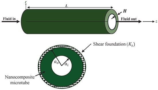
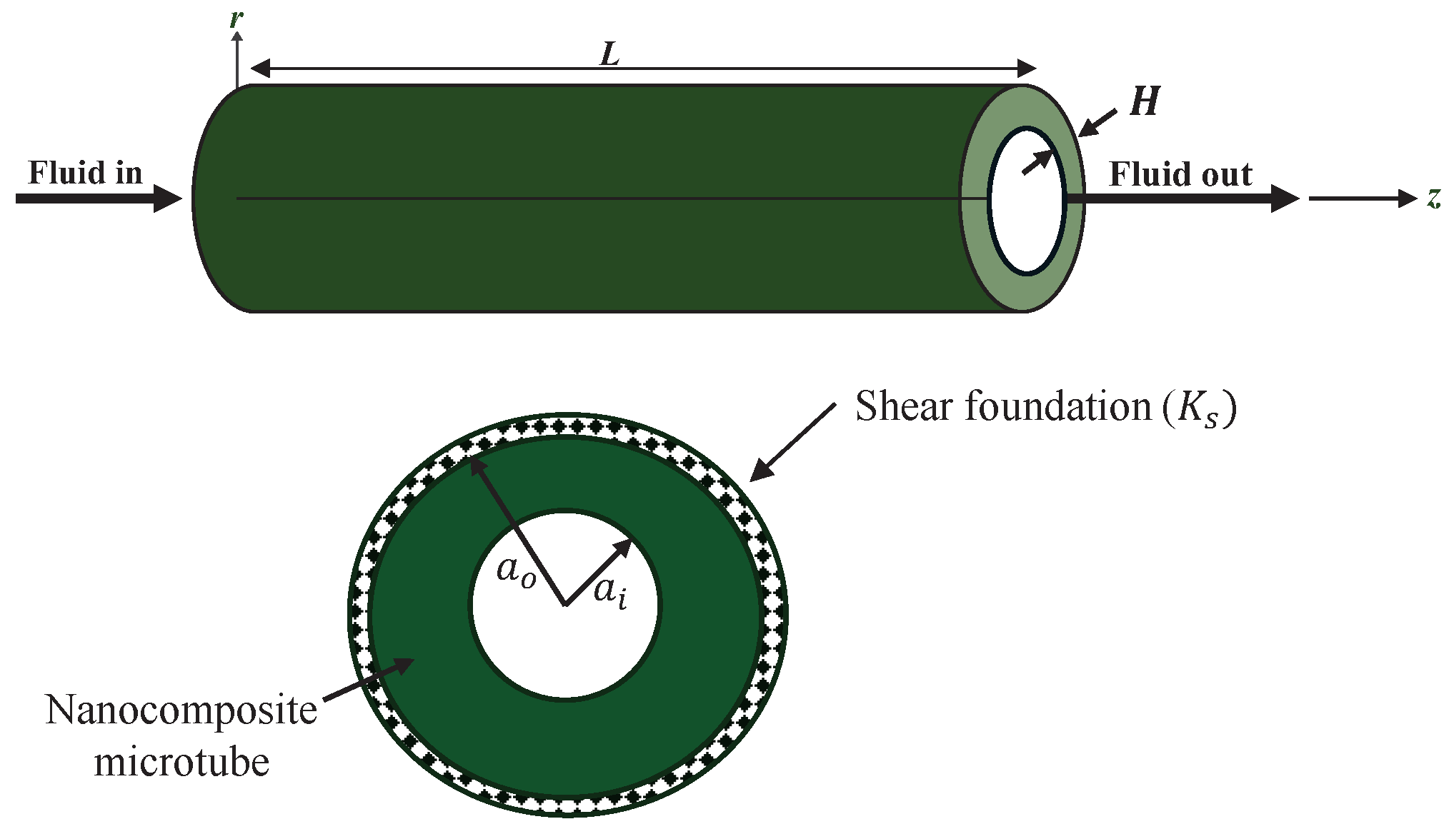
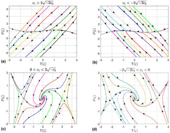
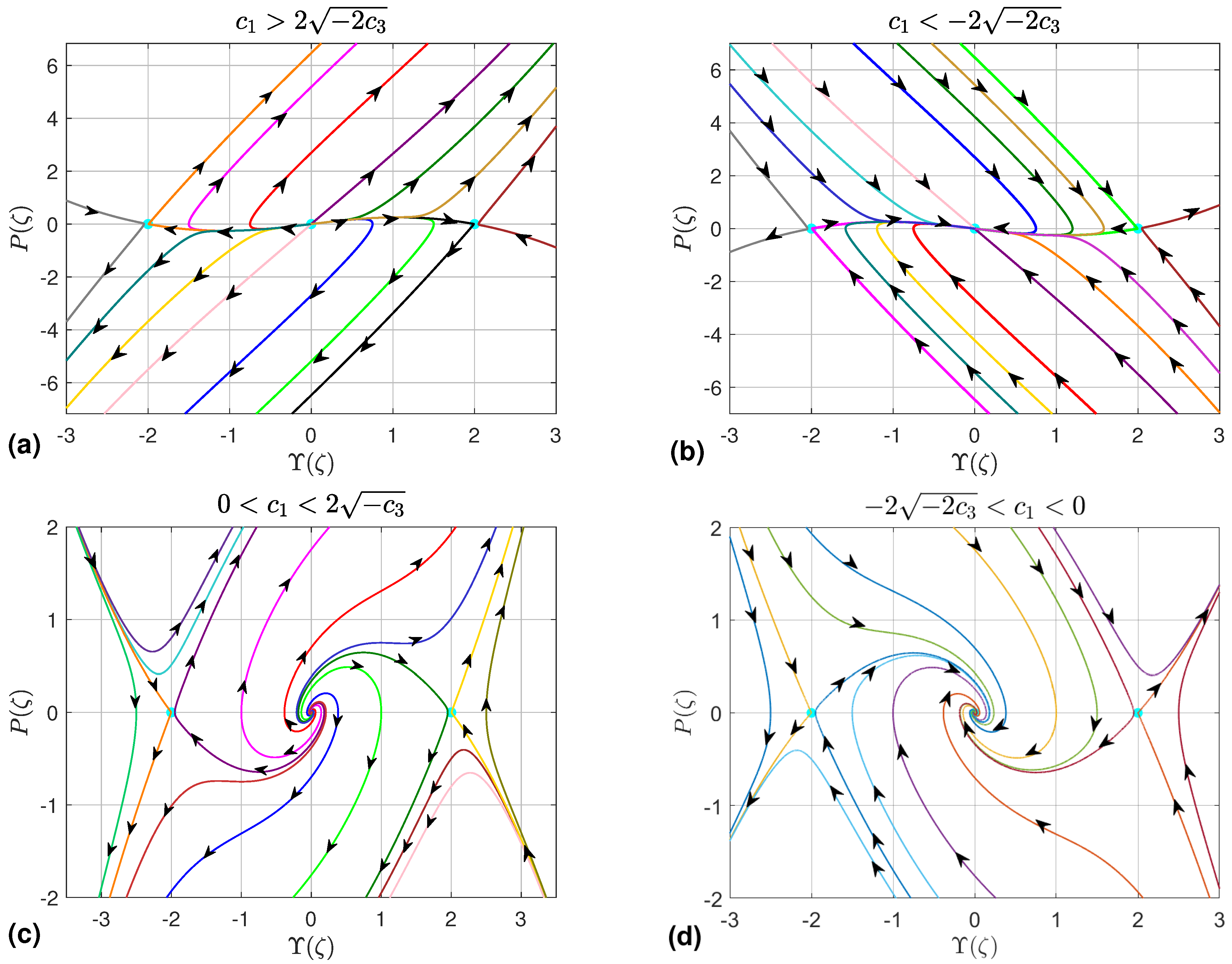
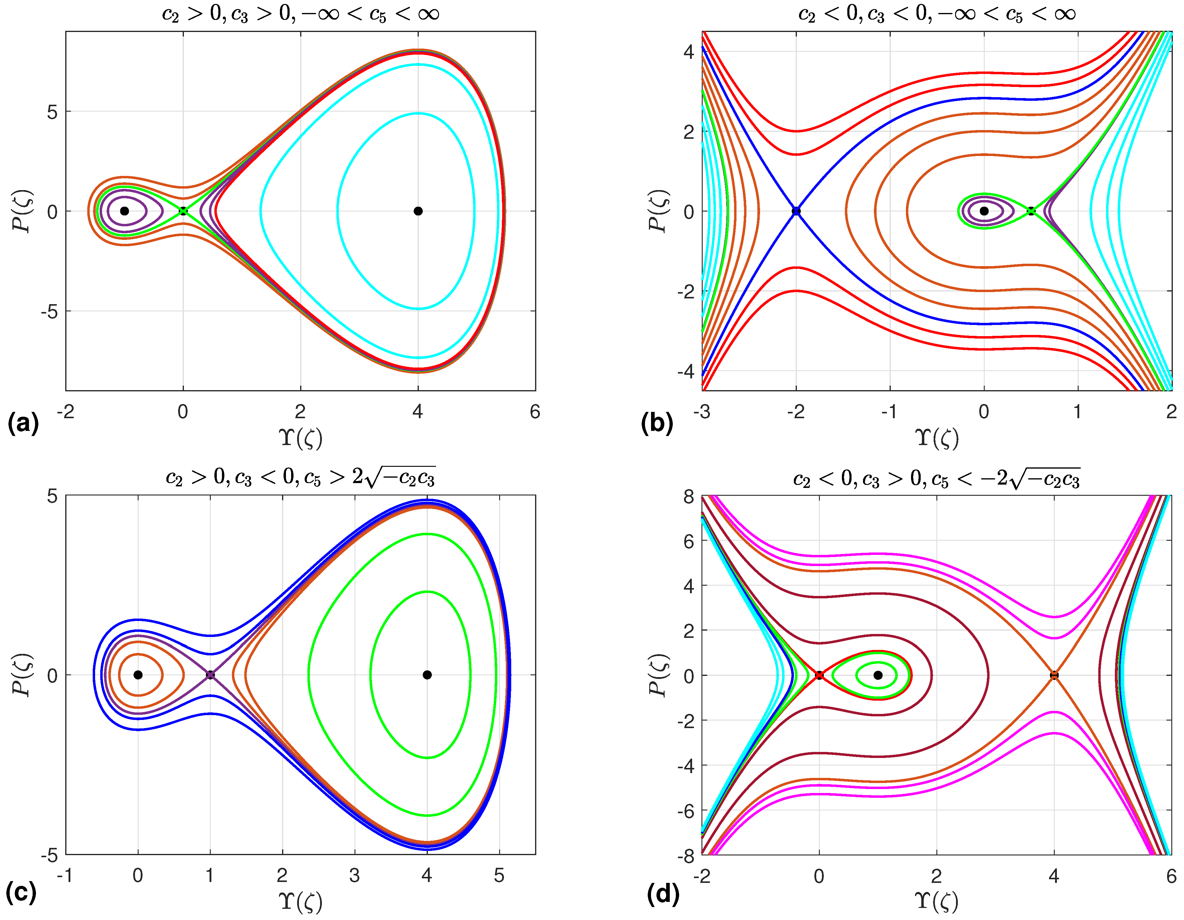
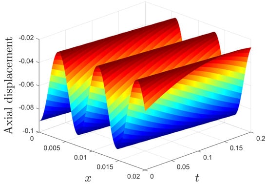
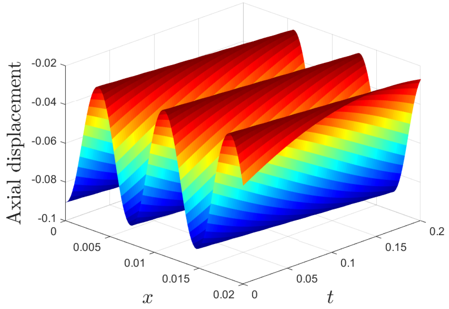
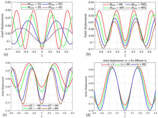
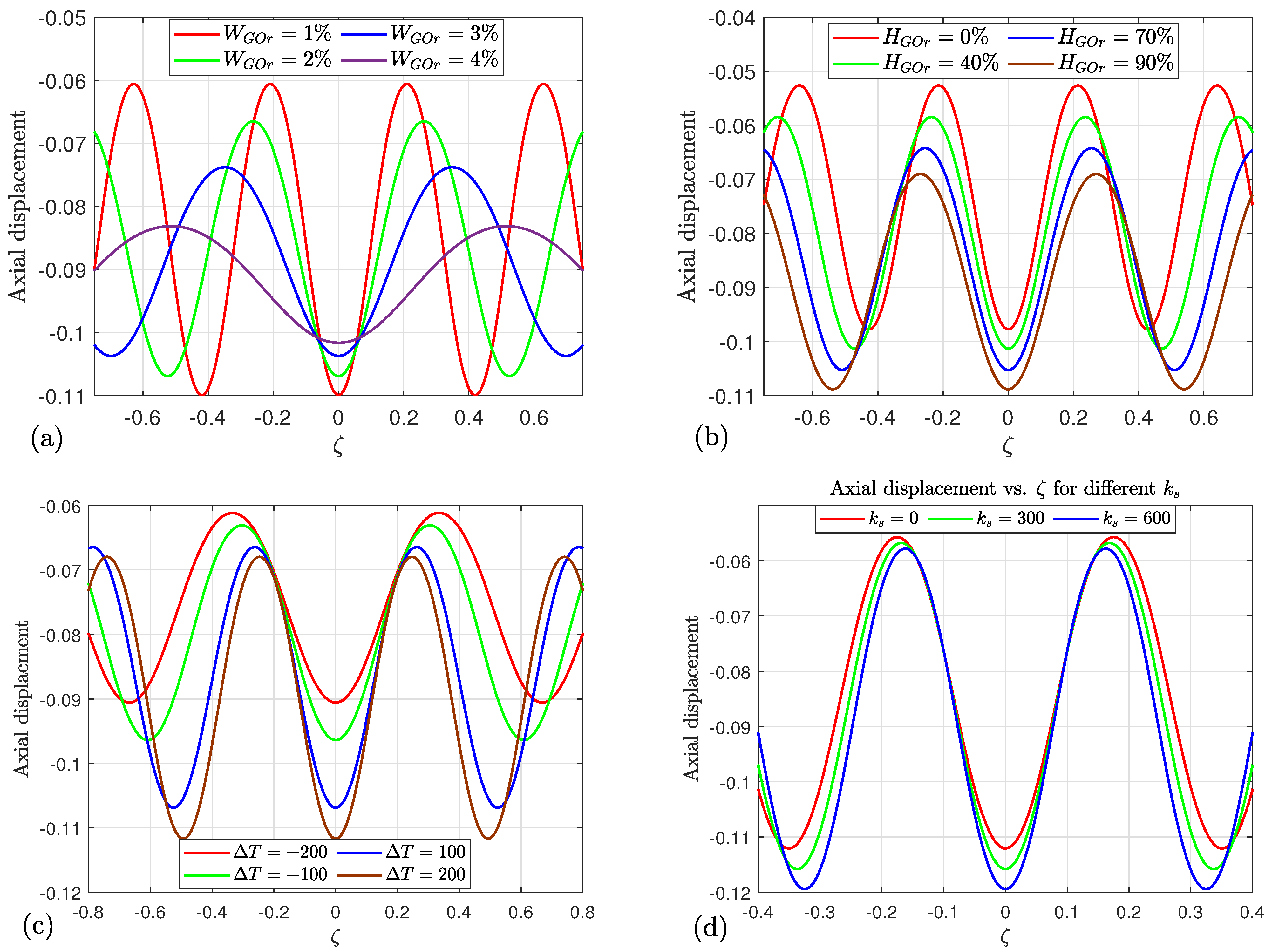
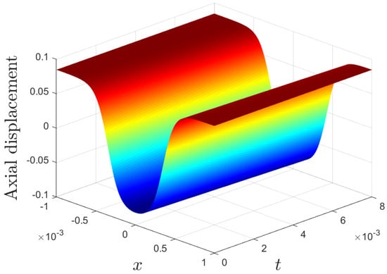
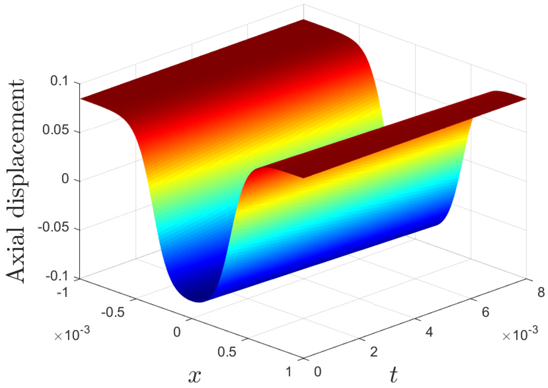
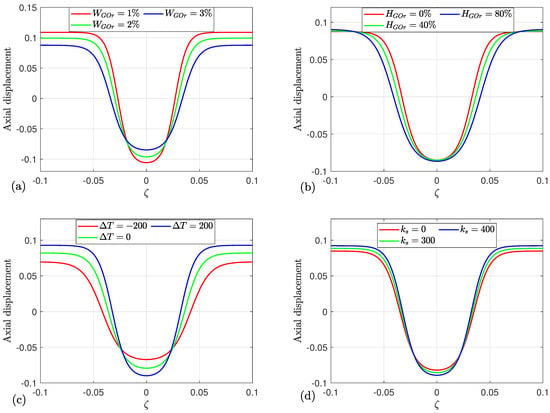
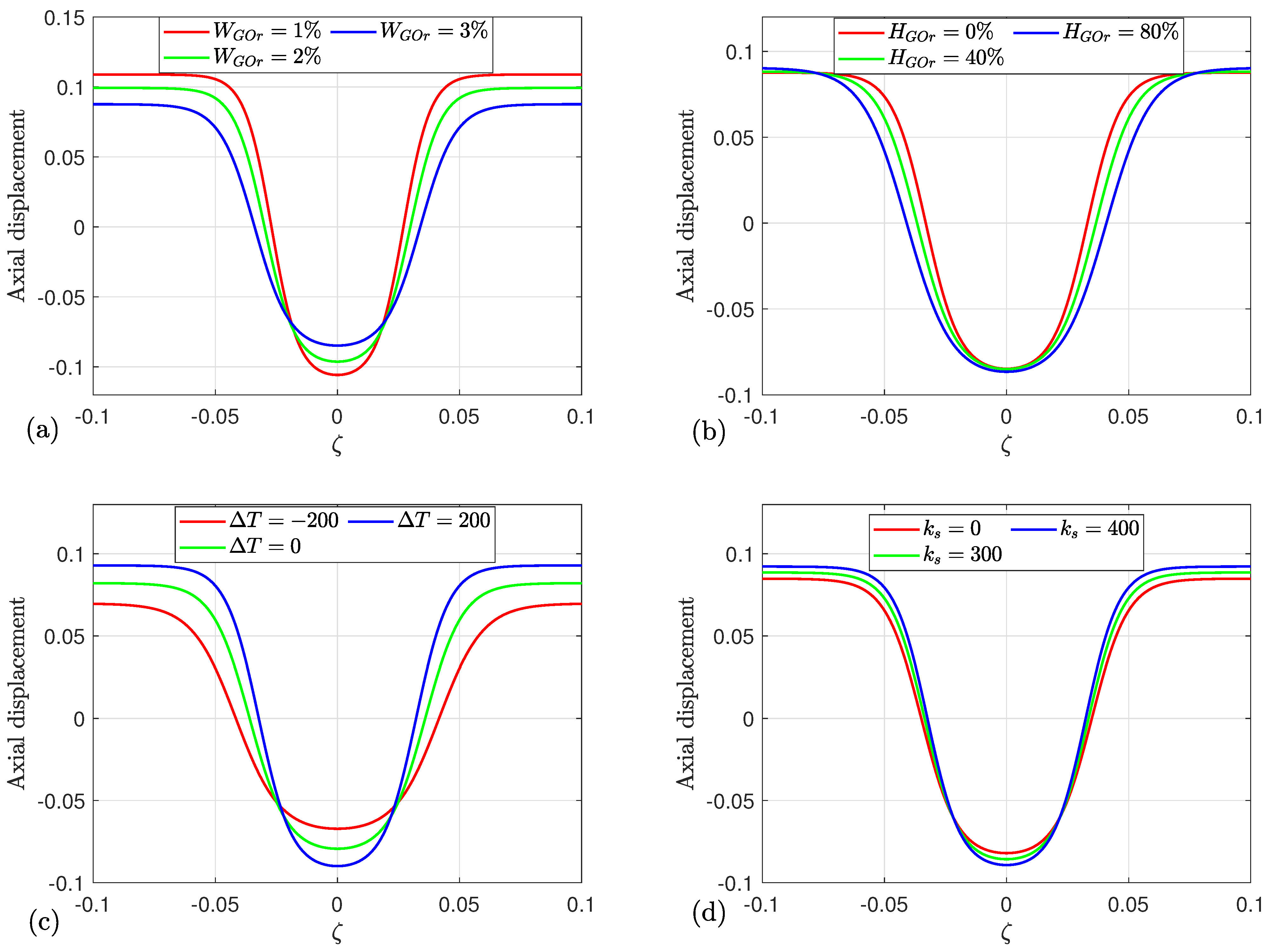
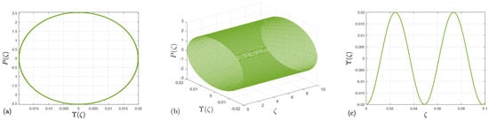
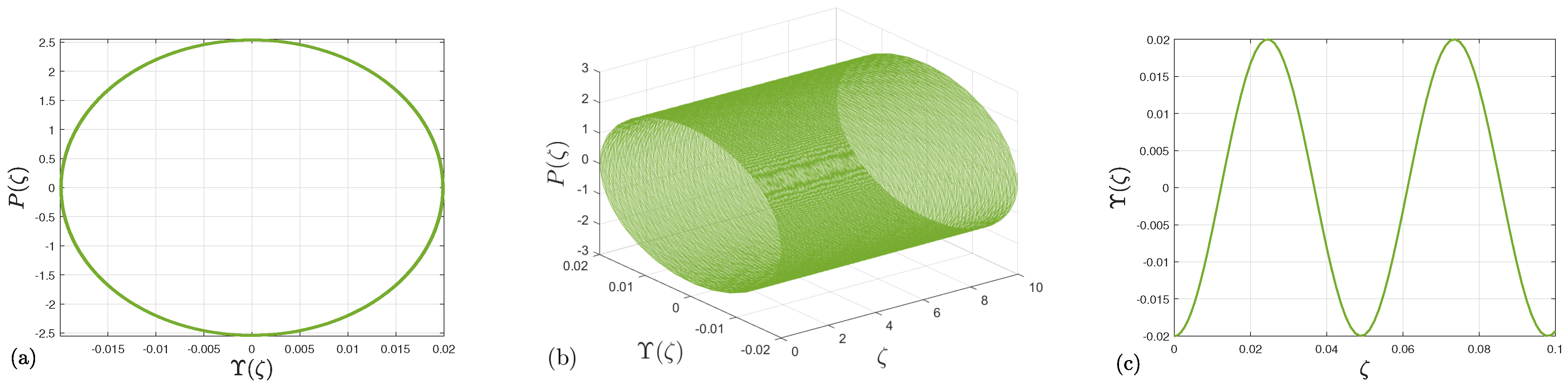
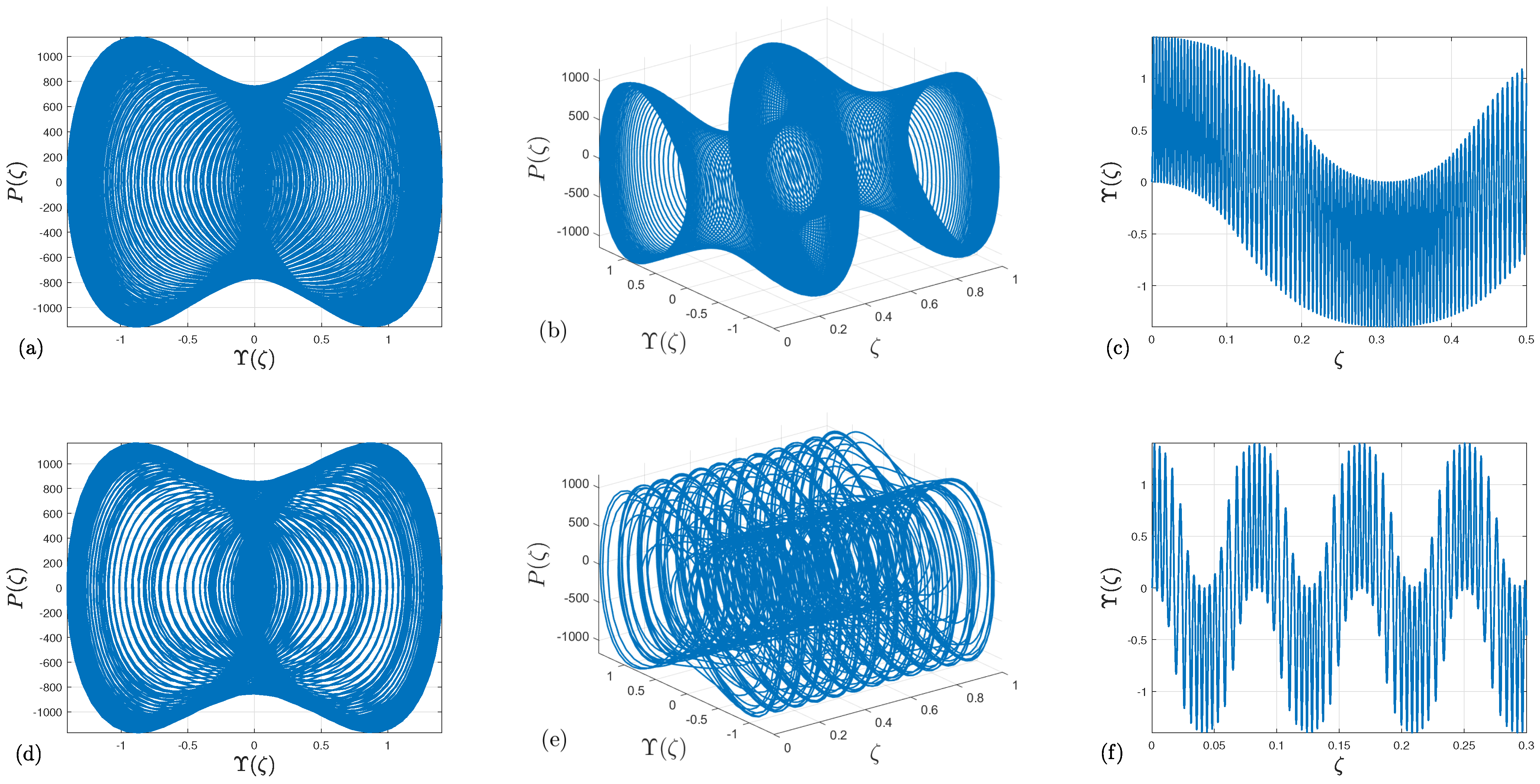
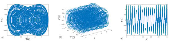
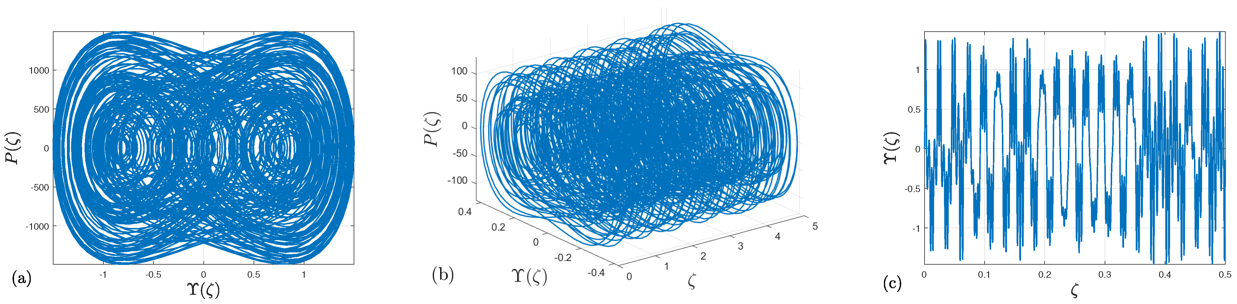
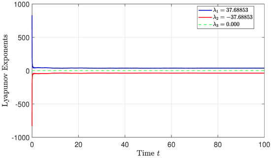
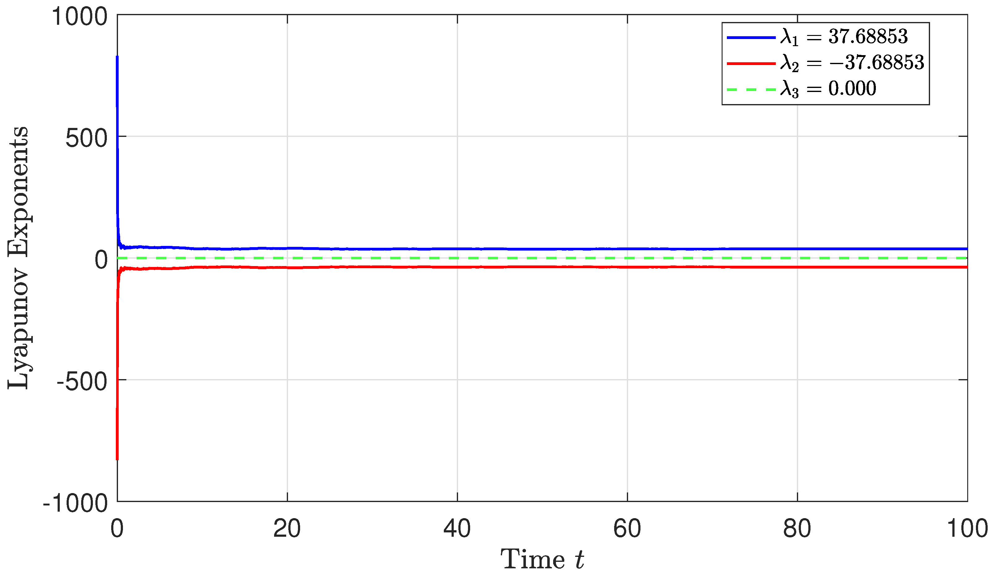
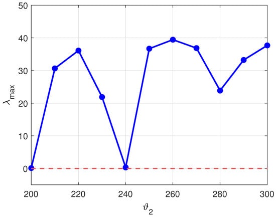
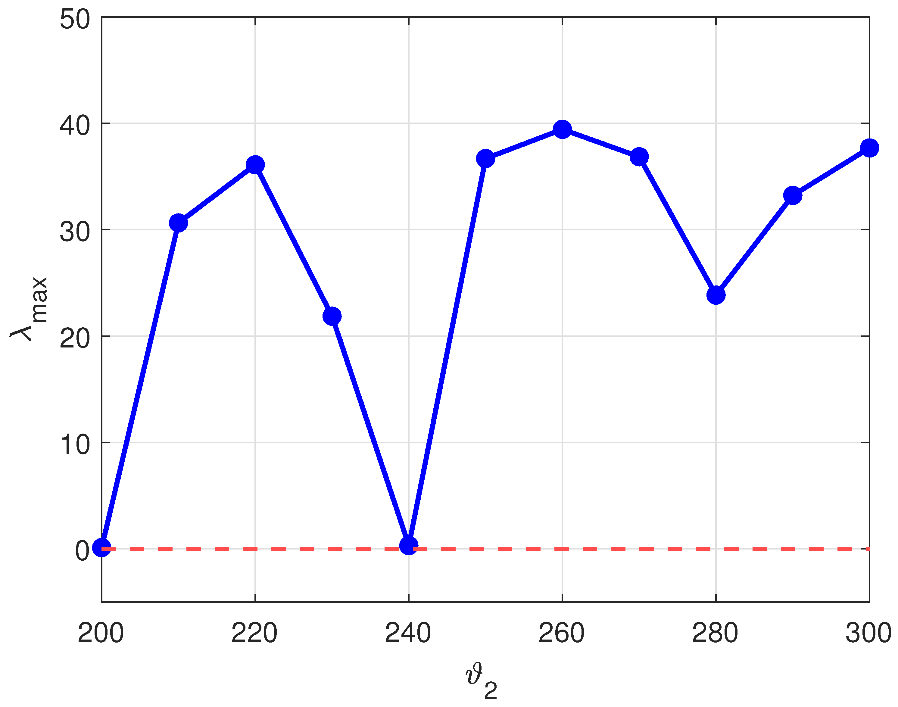
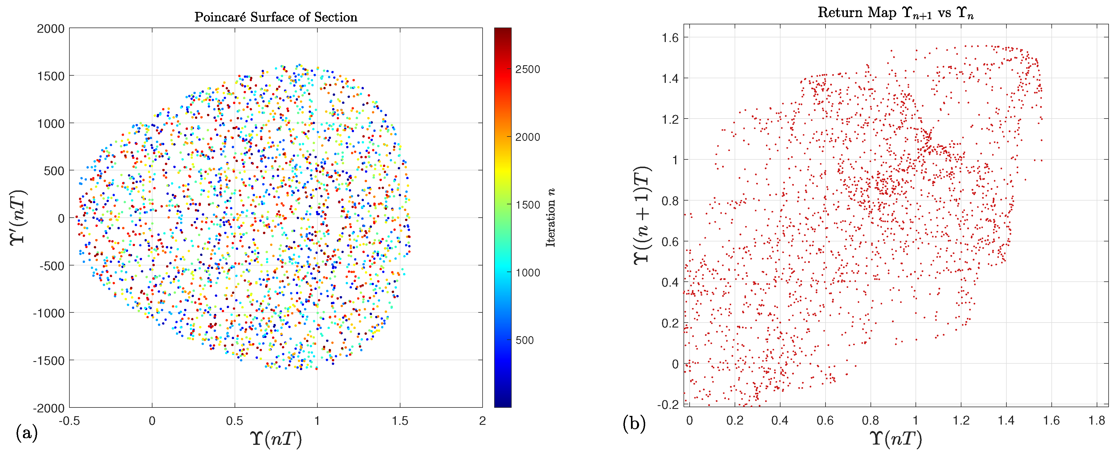

Disclaimer/Publisher’s Note: The statements, opinions and data contained in all publications are solely those of the individual author(s) and contributor(s) and not of MDPI and/or the editor(s). MDPI and/or the editor(s) disclaim responsibility for any injury to people or property resulting from any ideas, methods, instructions or products referred to in the content. |
© 2026 by the authors. Licensee MDPI, Basel, Switzerland. This article is an open access article distributed under the terms and conditions of the Creative Commons Attribution (CC BY) license.