Sparse Projection Attention: A Computationally Efficient Framework for Long Sequence Modeling

Abstract

The self-attention mechanism has revolutionized sequence modeling but suffers from quadratic computational complexity with respect to sequence length, limiting its applicability to long sequences. We propose Sparse Projection Attention (SPA), a novel attention variant that leverages learnable sparse projections to reduce the effective dimensionality of queries and keys while maintaining expressive power. Our method is grounded in the Johnson–Lindenstrauss lemma and provides theoretical guarantees on distance preservation for fixed random projection variants. We introduce a comprehensive mathematical framework including error bounds, convergence analysis, and gradient dynamics. Experimental results on language modeling, machine translation, and long-range sequence classification demonstrate that SPA achieves up to $8\times$ speedup in attention score computation, and approximately $2\times$ end-to-end speedup, while maintaining competitive performance compared to standard attention and other efficient variants. The proposed approach offers an effective trade-off between computational efficiency and model expressivity for long-sequence tasks, making transformers more accessible for resource-constrained environments and real-time applications.

1. Introduction

The Transformer architecture [1] has emerged as the dominant paradigm in modern deep learning, achieving state-of-the-art performance across diverse domains including natural language processing [2,3], computer vision [4,5], and speech processing [6]. At the heart of this architecture lies the self-attention mechanism, which enables the model to capture global dependencies by computing pairwise interactions between all positions in a sequence.

Despite its remarkable success, the standard self-attention mechanism exhibits quadratic computational complexity $\mathcal{O}\left(N^2{d}_k\right)$ and memory requirements $\mathcal{O}\left(N^2\right)$ with respect to sequence length N, where $d_k$ represents the dimensionality of queries and keys. This computational bottleneck becomes particularly problematic for long sequences encountered in domains such as document understanding [7], genomic sequence analysis [8], high-resolution image processing [5], and long-term temporal forecasting [9].

The limitations of standard attention have motivated extensive research into efficient alternatives. Current approaches can be broadly categorized into:

• Pattern-based Sparse Attention [10,11];
• Low-rank Approximations [12,13];
• Locality-Sensitive Hashing [14];
• Kernel-Based Methods [15,16].

1.1. Precise Positioning Against Related Work

SPA is related to but conceptually distinct from existing projection-based efficient attention methods in three important ways.

(i) vs. Linformer [12]. Linformer projects the key and value matrices along the sequence dimension from N to a fixed rank k, achieving $\mathcal{O}\left(Nk\right)$ complexity. SPA instead projects the feature dimension $d_k$ of both queries and keys symmetrically, preserving the full $N\times N$ attention structure. These are fundamentally different trade-offs: Linformer sacrifices per-token interaction fidelity; SPA reduces the inner-product space dimensionality while retaining all pairwise interactions.

(ii) vs. Performer [15]. Performer approximates $\mathrm{softmax}\left(Q{K}^T\right)$ via random feature maps (FAVOR+), effectively approximating the attention matrix itself at $\mathcal{O}\left(N\right)$ cost. SPA reduces the inner-product space in which scores are computed, provides JL-style guarantees for fixed random projections, and supports learnable sparse patterns, which Performer does not.

(iii) vs. Nyströmformer [17]. Nyströmformer approximates the attention matrix using a data-dependent Nyström decomposition with m landmark tokens. SPA operates in query- and key-feature space before score computation, is independent of token selection, and provides input-agnostic theoretical guarantees for its random projection variants.

1.2. Additional Related Work

Random Feature Attention [18] approximates the full attention map at $\mathcal{O}\left(N\right)$ cost but does not support learnable sparse patterns. Scatterbrain [19] combines sparse and low-rank approximations of the attention matrix; SPA is complementary as its projection operates in feature space. cosFormer [20] achieves $\mathcal{O}\left(N\right)$ complexity via cosine-based re-weighting. We refer the reader to the comprehensive survey by Tay et al. [21] for broader context. SPA is the only method that (a) projects both Q and K symmetrically in feature space, (b) provides JL-style guarantees for fixed projections, and (c) supports end-to-end learnable sparse patterns. A conceptual comparison is provided in Table 1.

Table 1. Conceptual comparison of SPA with related projection-based efficient attention methods. ^† JL guarantees apply to fixed random projection variants (SPA-Random, SPA-Block, SPA-Banded) only.

Method	Projected	JL	Learnable	Complexity
Linformer	$K,V$ seq. dim	No	No	$\mathcal{O}\left(N{d}_k\right)$
Performer	Attn. matrix	No	No	$\mathcal{O}\left(N{d}_{k}m\right)$
Nyströmformer	Attn. matrix	No	No	$\mathcal{O}\left(N{d}_k\right)$
SPA (Ours)	$Q,K$ feat. dim	Yes †	Yes	$\mathcal{O}\left(N^2{d}_k^{\prime }\right)$

In this paper, we introduce Sparse Projection Attention (SPA). The key contributions are:

• A mathematically grounded sparse projection mechanism reducing score computation to $\mathcal{O}\left(N^2{d}_k^{\prime }\right)$, with JL guarantees for fixed random projection variants;
• Comprehensive theoretical analysis including error bounds, convergence properties, and generalization bounds for the projection component;
• An adaptive sparsity learning algorithm;
• Extensive empirical evaluation demonstrating competitive performance with significant computational savings;
• Detailed ablation studies.

2. Theoretical Foundations

2.1. Johnson–Lindenstrauss Lemma and Random Projections

The Johnson–Lindenstrauss (JL) lemma [22] forms the cornerstone of our theoretical framework.

Lemma 1

(Johnson–Lindenstrauss). For any $0<ϵ<1$ and set X of m points in ${\mathbb{R}}^d$, there exists a linear map $f:{\mathbb{R}}^d\to {\mathbb{R}}^k$ with $k=\mathcal{O}({ϵ}^{-2}logm)$ such that for all $u,v\in X$:

$${(1-ϵ)\parallel u-v\parallel }^2\le {\parallel f\left(u\right)-f\left(v\right)\parallel }^2\le (1+ϵ){\parallel u-v\parallel }^2.$$

Theorem 1

(JL for Attention Preservation). Let $Q,K\in {\mathbb{R}}^{N\times d_k}$. For any $ϵ,\delta >0$, there exists $S\in {\mathbb{R}}^{d_k\times d_k^{\prime }}$ with $d_k^{\prime }=\mathcal{O}({ϵ}^{-2}log(N/\delta ))$ such that with probability $\ge 1-\delta$, for all $i,j\in \left[N\right]$:

$$\left|{\displaystyle \frac{⟨q_i,k_j⟩}{\sqrt{d_k}}}-{\displaystyle \frac{⟨q_{i}S,k_{j}S⟩}{\sqrt{d_k^{\prime }}}}\right|\le {\displaystyle \frac{ϵ}{2}}\left(\parallel q_i{\parallel }^2+{\parallel k_j\parallel }^2\right).$$

Proof. 

Step 1: Distribution of $\mathit{S}$. Let $S\in {\mathbb{R}}^{d_k\times d_k^{\prime }}$ have i.i.d. $\sigma$-sub-Gaussian entries with ${\sigma }^2=1/d_k^{\prime }$ (e.g., $S_{ij}\sim \mathcal{N}(0,1/d_k^{\prime })$). By the quantitative JL lemma [23], for any fixed vector u and failure probability $\eta \in (0,1)$:

$$\mathbb{P}\left[(1-{ϵ}^{\prime }){\parallel u\parallel }^2\le {\parallel uS\parallel }^2\le (1+{ϵ}^{\prime }){\parallel u\parallel }^2\right]\ge 1-\eta .$$

Step 2: From distances to inner products (polarization identity). For all $i,j\in \left[N\right]$, the polarization identity gives

$$⟨q_i,k_j⟩=\frac{1}{4}\left(\parallel q_i+k_j{\parallel }^2-{\parallel q_i-k_j\parallel }^2\right),$$

and analogously $⟨q_{i}S,k_{j}S⟩=\frac{1}{4}(\parallel (q_i+k_j){S\parallel }^2-\parallel (q_i-k_j)S{\parallel }^2)$. Set $u^{+}=q_i+k_j$ and $u^{-}=q_i-k_j$, and apply Step 1 to each of these vectors: with probability at least $1-2\eta$,

$$\left|\parallel u^{\pm }{S\parallel }^2-{\parallel u^{\pm }\parallel }^2\right|\le {ϵ}^{\prime }{\parallel u^{\pm }\parallel }^2.$$

Combining via the polarization identity and using $\parallel u^{+}{\parallel }^2+\parallel u^{-}{\parallel }^2=2(\parallel q_i{\parallel }^2+\parallel k_j{\parallel }^2)$ yields

$$\left|⟨q_{i}S,k_{j}S⟩-⟨q_i,k_j⟩\right|\le \frac{{ϵ}^{\prime }}{4}\left(\parallel u^{+}{\parallel }^2+{\parallel u^{-}\parallel }^2\right)=\frac{{ϵ}^{\prime }}{2}\left(\parallel q_i{\parallel }^2+{\parallel k_j\parallel }^2\right).$$

(1)

This is the natural symmetric bound delivered by the polarization identity, and it is the form we adopt throughout.

Step 3: Union bound. Set ${\eta }_{ij}=\delta /\left(2N^2\right)$ in Step 1 applied to each of the $2N^2$ vectors ${\{u_{ij}^{+},u_{ij}^{-}\}}_{i,j\in \left[N\right]}$. By union bound, all inequalities hold simultaneously with probability $\ge 1-\delta$, requiring $d_k^{\prime }=\mathcal{O}({ϵ}^{-2}log(N/\delta ))$.

Step 4: Normalization. From Step 2 (Equation (1)),

$$|⟨q_{i}S,k_{j}S⟩-⟨q_i,k_j⟩|\le \frac{{ϵ}^{\prime }}{2}\left(\parallel q_i{\parallel }^2+{\parallel k_j\parallel }^2\right).$$

By the triangle inequality:

$$\left|{\displaystyle \frac{⟨q_i,k_j⟩}{\sqrt{d_k}}}-{\displaystyle \frac{⟨q_{i}S,k_{j}S⟩}{\sqrt{d_k^{\prime }}}}\right|\le {\displaystyle \frac{|⟨q_i,k_j⟩-⟨q_{i}S,k_{j}S⟩|}{\sqrt{d_k}}}+\left|⟨q_{i}S,k_{j}S⟩\right|·\left|{\displaystyle \frac{1}{\sqrt{d_k}}}-{\displaystyle \frac{1}{\sqrt{d_k^{\prime }}}}\right|.$$

The first term is bounded by ${\displaystyle \frac{{ϵ}^{\prime }}{2\sqrt{d_k}}}(\parallel q_i{\parallel }^2+ \parallel k_j{\parallel }^2) \le {\displaystyle \frac{{ϵ}^{\prime }}{2}}(\parallel q_i{\parallel }^2+ \parallel k_j{\parallel }^2)$. For the second, the Cauchy–Schwarz inequality and Step 1 give $|⟨q_{i}S,k_{j}S⟩| \le \parallel q_{i}S\parallel \parallel k_{j}S\parallel \le (1+{ϵ}^{\prime })\parallel q_i\parallel \parallel k_j\parallel \le \frac{1+{ϵ}^{\prime }}{2}(\parallel q_i{\parallel }^2+ \parallel k_j{\parallel }^2)$ (using AM-GM in its correct direction $\parallel q_i\parallel \parallel k_j\parallel \le \frac{1}{2}(\parallel q_i{\parallel }^2+ \parallel k_j{\parallel }^2)$), while $\left|1/\sqrt{d_k}-1/\sqrt{d_k^{\prime }}\right|\le 1/\sqrt{d_k^{\prime }}$ since $d_k^{\prime }\le d_k$. Setting ${ϵ}^{\prime }=ϵ/(2+2ϵ)\approx ϵ/2$ and absorbing constants into $O\left(d_k^{\prime }\right)$ yields the bound ${\displaystyle \frac{ϵ}{2}}(\parallel q_i{\parallel }^2+ \parallel k_j{\parallel }^2)$.    □

Remark 1

(Product form under norm normalization). Under the standard normalization $\parallel q_i\parallel ,\parallel k_j\parallel \le 1$ enforced by LayerNorm in Transformer architectures, AM-GM gives $\parallel q_i\parallel \parallel k_j\parallel \le \frac{1}{2}(\parallel q_i{\parallel }^2+ \parallel k_j{\parallel }^2)\le 1$, so the symmetric bound of Theorem 1 implies the product form

$$\left|{\displaystyle \frac{⟨q_i,k_j⟩}{\sqrt{d_k}}}-{\displaystyle \frac{⟨q_{i}S,k_{j}S⟩}{\sqrt{d_k^{\prime }}}}\right|\le ϵ.$$

We use the symmetric form throughout the analysis since it is distribution-free; the product form is invoked only when explicitly indicated.

Remark 2

(Scope of JL-Based Guarantees). The guarantees of Theorem 1 rely on S being drawn from a sub-Gaussian distribution and remaining fixed. They apply rigorously to SPA-Random, SPA-Block, and SPA-Banded. For SPA-Learn and SPA-Adaptive, S is initialized randomly but subsequently optimized by gradient descent; after training it is deterministic and data-dependent, and no longer satisfies the JL distributional assumptions. The theoretical treatment of learnable variants is provided in Section 4.4.

2.2. Sparse Random Projections

Definition 1

(Sparse Random Matrix). A sparse random matrix $S\in {\mathbb{R}}^{d_k\times d_k^{\prime }}$ has entries:

$$S_{ij}=\sqrt{{\displaystyle \frac{s}{d_k^{\prime }}}}\times \left\{\begin{array}{cc}+1\hfill & \mathit{with}\mathit{probability}{\displaystyle \frac{1}{2s}}\hfill \\ 0\hfill & \mathit{with}\mathit{probability}1-{\displaystyle \frac{1}{s}}\hfill \\ -1\hfill & \mathit{with}\mathit{probability}{\displaystyle \frac{1}{2s}},\hfill \end{array}\right.$$

where $s\ge 1$ controls the sparsity level.

Proposition 1

(Sparse JL Guarantee). For the sparse random matrix of Definition 1 with $s=\mathcal{O}\left(\sqrt{d_k}\right)$ and $d_k^{\prime }=\mathcal{O}({ϵ}^{-2}logN)$, the distance preservation guarantee of Lemma 1 holds with high probability.

Proof. 

The distance preservation bound is established in Achlioptas [24], Theorem 1.1: for m points and $ϵ\in (0,1)$, choosing $d_k^{\prime }\ge C{ϵ}^{-2}logm$ ensures $(1\pm ϵ)$-isometry with probability $\ge 1-m^{-\beta }$. Setting $m=2N^2$ (union bound over all query-key pairs and their sums and differences as in Theorem 1) gives $d_k^{\prime }=\mathcal{O}({ϵ}^{-2}logN)$. The computational gain follows from sparsity: each column of S has on average $d_k/s$ nonzero entries, reducing the projection cost to $\mathcal{O}(N{d}_k{d}_k^{\prime }/s)$.    □

Corollary 1

(Sparse JL for Attention Scores). Under the conditions of Proposition 1, the attention score preservation guarantee of Theorem 1 holds for the sparse matrix S of Definition 1.

Proof. 

The distance preservation of Proposition 1 implies inner-product preservation via the polarization identity (Step 2 of Theorem 1). Theorem 1 then follows by Lemma 1 and the same argument as for dense projections.    □

2.3. Attention Score Preservation

Lemma 2

(Softmax Lipschitz in Frobenius Norm). Let $\mathrm{softmax}:{\mathbb{R}}^{N\times N}\to {\mathbb{R}}^{N\times N}$ be applied row-wise. For any $A,B\in {\mathbb{R}}^{N\times N}$:

$${\parallel \mathrm{softmax}\left(A\right)-\mathrm{softmax}\left(B\right)\parallel }_F\le {\parallel A-B\parallel }_F.$$

Proof. 

For each row i, the Jacobian of $\mathrm{softmax}$ at $a\in {\mathbb{R}}^N$ is $J_a=\mathrm{diag}\left(p\right)-p{p}^T$ with $p=\mathrm{softmax}\left(a\right)$. All eigenvalues of $J_a$ lie in $[0,1]$, so ${\parallel J_a\parallel }_2\le 1$. Since $\mathrm{softmax}$ maps ${\mathbb{R}}^N$ to the probability simplex ${\Delta }^{N-1}$, which is compact and convex, the mean-value theorem applies: for any segment $[a,b]$ there exists $c\in [a,b]$ such that ${\parallel \mathrm{softmax}\left(a\right)-\mathrm{softmax}\left(b\right)\parallel }_2= \parallel J_c{(a-b)\parallel }_2\le \parallel J_c{\parallel }_2{\parallel a-b\parallel }_2\le {\parallel a-b\parallel }_2$. Summing over rows: ${\parallel \mathrm{softmax}\left(A\right)-\mathrm{softmax}\left(B\right)\parallel }_F^2\le {\sum }_i\parallel A_i-B_i{\parallel }_2^2 ={\parallel A-B\parallel }_F^2$.    □

Theorem 2

(Attention Score Preservation). Let $Q,K\in {\mathbb{R}}^{N\times d_k}$ and $S\in {\mathbb{R}}^{d_k\times d_k^{\prime }}$ be a sparse random projection. For any $ϵ>0$ and $\delta \in (0,1)$, with probability $\ge 1-\delta$:

$${∥\mathrm{softmax}\left({\displaystyle \frac{Q{K}^T}{\sqrt{d_k}}}\right)-\mathrm{softmax}\left({\displaystyle \frac{QS{S}^T{K}^T}{\sqrt{d_k^{\prime }}}}\right)∥}_F\le {C\parallel Q\parallel }_F{\parallel K\parallel }_F\sqrt{{\displaystyle \frac{log(N/\delta )}{d_k^{\prime }}}}\left({\displaystyle \frac{1}{\sqrt{d_k}}}+{\displaystyle \frac{1}{\sqrt{d_k^{\prime }}}}\right),$$

where $C>0$ is a universal constant.

Proof. 

Let $A_{\mathrm{raw}}=Q{K}^T/\sqrt{d_k}$ and ${\tilde{A}}_{\mathrm{raw}}=QS{S}^T{K}^T/\sqrt{d_k^{\prime }}$. By Lemma 2: $\parallel \mathrm{softmax}\left(A_{\mathrm{raw}}\right)-\mathrm{softmax}\left({\tilde{A}}_{\mathrm{raw}}\right){\parallel }_F \le {\parallel A_{\mathrm{raw}}-{\tilde{A}}_{\mathrm{raw}}\parallel }_F$. By the triangle inequality:

$$\parallel A_{\mathrm{raw}}-{\tilde{A}}_{\mathrm{raw}}{\parallel }_F \le {\displaystyle \frac{\parallel Q{K}^T-QS{S}^T{K}^T{\parallel }_F}{\sqrt{d_k}}}+{\parallel QS{S}^T{K}^T\parallel }_F·\left|{\displaystyle \frac{1}{\sqrt{d_k}}}-{\displaystyle \frac{1}{\sqrt{d_k^{\prime }}}}\right|.$$

Bounding the first term. From Theorem 1 with ${ϵ}_0=C^{\prime }\sqrt{log(N/\delta )/d_k^{\prime }}$, with probability $\ge 1-\delta$, for all $i,j$: $|{\left(Q{K}^T\right)}_{ij}-{\left(QS{S}^T{K}^T\right)}_{ij}| \le {ϵ}_0\parallel q_i\parallel \parallel k_j\parallel$. Squaring and summing:

$$\parallel Q{K}^T-QS{S}^T{K}^T{\parallel }_F^2 = \sum _{i,j}|{\left(Q{K}^T\right)}_{ij}-{\left(QS{S}^T{K}^T\right)}_{ij}{|}^2\le {ϵ}_0^2\sum _{i,j}\parallel q_i{\parallel }^2\parallel k_j{\parallel }^2 = {ϵ}_0^2{\parallel Q\parallel }_F^2{\parallel K\parallel }_F^2.$$

Hence the first term is $\le {ϵ}_0{\parallel Q\parallel }_F{\parallel K\parallel }_F/\sqrt{d_k}$.

Bounding the second term. By sub-multiplicativity and Proposition 1 (norm preservation): $\parallel QS{S}^T{K}^T{\parallel }_F \le {\parallel QS\parallel }_F{\parallel KS\parallel }_F\le {(1+{ϵ}_0)}^2{\parallel Q\parallel }_F{\parallel K\parallel }_F\le {4\parallel Q\parallel }_F{\parallel K\parallel }_F$ for ${ϵ}_0\le 1$. Since $d_k^{\prime }\le d_k$: $|1/\sqrt{d_k}-1/\sqrt{d_k^{\prime }}| \le 1/\sqrt{d_k^{\prime }}$.

Combining and identifying C. Adding both terms:

$$\begin{array}{cc}\hfill \parallel \mathrm{softmax}\left(A_{\mathrm{raw}}\right)-\mathrm{softmax}\left({\tilde{A}}_{\mathrm{raw}}\right){\parallel }_F& \le {\displaystyle \frac{{ϵ}_0{\parallel Q\parallel }_F{\parallel K\parallel }_F}{\sqrt{d_k}}}+{\displaystyle \frac{{4\parallel Q\parallel }_F{\parallel K\parallel }_F}{\sqrt{d_k^{\prime }}}}\hfill \\ \hfill & \le {C\parallel Q\parallel }_F{\parallel K\parallel }_F\sqrt{{\displaystyle \frac{log(N/\delta )}{d_k^{\prime }}}}\left({\displaystyle \frac{1}{\sqrt{d_k}}}+{\displaystyle \frac{1}{\sqrt{d_k^{\prime }}}}\right),\hfill \end{array}$$

where $C=max(C^{\prime },4/\sqrt{log(N/\delta )})$.    □

3. Sparse Projection Attention Model

3.1. Mathematical Formulation

3.1.1. Standard Attention Recap

$\mathrm{Attention}(Q,K,V)=\mathrm{softmax}(Q{K}^T/\sqrt{d_k})V$, with bottleneck $Q{K}^T$ at cost $\mathcal{O}\left(N^2{d}_k\right)$.

3.1.2. Sparse Projection Layer

$Q^{\prime }=QS,K^{\prime }=KS,Q^{\prime },K^{\prime }\in {\mathbb{R}}^{N\times d_k^{\prime }}$.

3.1.3. Sparse Projection Attention (SPA)

$$\mathrm{SPA}(Q,K,V)=\mathrm{softmax}\left({\displaystyle \frac{Q^{\prime }{\left(K^{\prime }\right)}^T}{\sqrt{d_k^{\prime }}}}\right)V.$$

Score complexity: $\mathcal{O}\left(N^2{d}_k^{\prime }\right)$, speedup $d_k/d_k^{\prime }$ over standard attention. The full end-to-end cost is analyzed in Section 4.1.

3.2. Sparsity Pattern Definitions

We introduce two families of sparsity patterns for the projection matrix S: fixed patterns, which preserve JL guarantees, and learnable patterns, which adapt to the task at the cost of formal theoretical guarantees.

• Fixed Sparsity Patterns: Random sparse, block sparse, banded sparse—all satisfying the JL guarantees of Theorem 1.
• Learnable Sparsity Patterns:$S_{ij}=M_{ij}·W_{ij}$ with binary mask M and learnable weights W. The mask is optimized via Gumbel-softmax reparameterization [25] with temperature annealed from 1.0 to 0.1, $L_0$ regularization, or magnitude pruning. Unlike fixed projections, learnable patterns are data-driven and the JL guarantees of Theorem 1 do not apply post-training (see Section 4.4).
• Structured Sparsity Patterns: Hierarchical, conv, and head-specific patterns.

3.3. Visual Architecture Overview

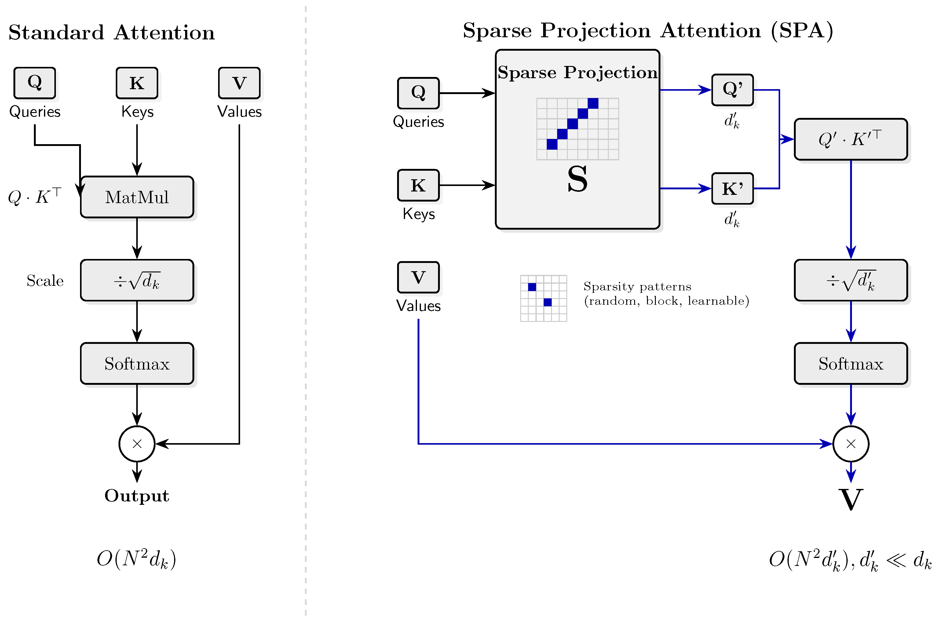
Figure 1 contrasts the standard self-attention pipeline with the proposed SPA. The key architectural difference is the insertion of a learnable (or random) sparse projection S that maps queries and keys from ${\mathbb{R}}^{d_k}$ to ${\mathbb{R}}^{d_k^{\prime }}$ before the attention-score computation. The projection S is shared across all positions in a given layer, so the additional memory cost is independent of the sequence length N.

Figure 1. Architecture comparison between standard self-attention (left) and Sparse Projection Attention (right). SPA reduces the feature dimension from $d_k$ to $d_k^{\prime }\ll d_k$, lowering score computation from $\mathcal{O}\left(N^2{d}_k\right)$ to $\mathcal{O}\left(N^2{d}_k^{\prime }\right)$.

3.4. Gradient Analysis and Training Dynamics

3.4.1. Gradient Flow

$${\nabla }_Q\mathcal{L}=\left({\nabla }_{Q^{\prime }}\mathcal{L}\right)S^T,{\nabla }_S\mathcal{L}=Q^T\left({\nabla }_{Q^{\prime }}\mathcal{L}\right).$$

3.4.2. Convergence Analysis

Assumption 1

(L-smoothness). $\parallel \nabla \mathcal{L}\left(\theta \right)-\nabla \mathcal{L}\left(\varphi \right)\parallel \le L\parallel \theta -\varphi \parallel$ for all $\theta ,\varphi \in \Theta$.

Assumption 2

(Bounded gradients). ${\mathbb{E}[\parallel \nabla \mathcal{L}\left(\theta \right)\parallel }^2]\le G^2$ for all $\theta \in \Theta$.

Assumption 3

(Bounded projection error). $\parallel \nabla \mathcal{L}\left(\theta \right)-\tilde{\nabla }\mathcal{L}\left(\theta \right)\parallel \le {\delta }_{ϵ}$, where ${\delta }_{ϵ}=C_1{ϵ\parallel Q\parallel }_F{\parallel K\parallel }_F$ and $C_1>0$.

Theorem 3

(SPA Convergence). Under Assumptions 1–3, with ${\eta }_t=\eta /\sqrt{T}$:

$${\displaystyle \frac{1}{T}}{\displaystyle \sum _{t=1}^T}\mathbb{E}\left[\parallel \nabla \mathcal{L}\left({\theta }_t\right){\parallel }^2\right]\le {\displaystyle \frac{2(\mathcal{L}\left({\theta }_0\right)-{\mathcal{L}}^{*})}{\eta \sqrt{T}}}+\eta L{G}^2+2G{\delta }_{ϵ}.$$

Proof. Step 1: Descent lemma. 

By L-smoothness: $\mathcal{L}\left({\theta }_{t+1}\right)\le \mathcal{L}\left({\theta }_t\right)-{\eta }_t⟨{\nabla }_t,{\tilde{\nabla }}_t⟩+{\displaystyle \frac{L{\eta }_t^2}{2}}{\parallel {\tilde{\nabla }}_t\parallel }^2$.

Step 2: Cross-term. By Cauchy-Schwarz and Assumptions 2 and 3: $⟨{\nabla }_t,{\tilde{\nabla }}_t⟩= \parallel {\nabla }_t{\parallel }^2+⟨{\nabla }_t,{\tilde{\nabla }}_t-{\nabla }_t⟩\ge \parallel {\nabla }_t{\parallel }^2-\parallel {\nabla }_t\parallel \parallel {\tilde{\nabla }}_t-{\nabla }_t\parallel \ge \parallel {\nabla }_t{\parallel }^2-G{\delta }_{ϵ}$.

Step 3: Quadratic term. $\parallel {\tilde{\nabla }}_t\parallel \le \parallel {\nabla }_t\parallel + {\delta }_{ϵ}\le G+{\delta }_{ϵ}\le 2G$ (for ${\delta }_{ϵ} \le G$), so $\parallel {\tilde{\nabla }}_t{\parallel }^2 \le 4G^2$.

Step 4: Substitution and summation. Substituting and summing over $t=1,\dots ,T$:

$${\displaystyle \sum _{t=1}^T}{\eta }_t{\parallel {\nabla }_t\parallel }^2\le \mathcal{L}\left({\theta }_0\right)-{\mathcal{L}}^{*}+G{\delta }_{ϵ}{\displaystyle \sum _{t=1}^T}{\eta }_t+2L{G}^2{\displaystyle \sum _{t=1}^T}{\eta }_t^2.$$

Step 5: Computing the sums. With ${\eta }_t=\eta /\sqrt{T}$: ${\sum }_{t=1}^T{\eta }_t=\eta \sqrt{T}$ and ${\sum }_{t=1}^T{\eta }_t^2={\eta }^2$. Dividing by $\eta \sqrt{T}$ yields the stated bound.    □

3.4.3. Interpretation of the Bound

The right-hand side of the bound decomposes into three contributions:

• an optimization term ${\displaystyle \frac{2(\mathcal{L}\left({\theta }_0\right)-{\mathcal{L}}^{*})}{\eta \sqrt{T}}}$, which decays as $\mathcal{O}(1/\sqrt{T})$ with the number of iterations;
• a step-size bias $\eta L{G}^2$, controlled by the learning rate $\eta$;
• a projection bias $2G{\delta }_{ϵ}$, controlled by the projection-error term ${\delta }_{ϵ}=C_1{ϵ\parallel Q\parallel }_F{\parallel K\parallel }_F$ from Assumption 3.

Convergence to a stationary point therefore requires both the step-size and the projection bias to vanish. This holds, for instance, under a decreasing learning-rate schedule ${\eta }_t={\eta }_0/\sqrt{t}$ combined with $d_k^{\prime }\to \infty$, since by Theorem 1 the projection error satisfies ${\delta }_{ϵ}=\mathcal{O}\left(\sqrt{log(N/\delta )/d_k^{\prime }}\right)\to 0$. With these two conditions, the algorithm converges to a stationary point of the true (unprojected) objective; with the constant schedule ${\eta }_t=\eta /\sqrt{T}$ used above, the bound only guarantees convergence to a stationary region whose radius is controlled by $\eta$ and $d_k^{\prime }$. This is consistent with classical results for perturbed SGD [26].

Scope note. This result is a corollary of general perturbed-SGD theory [26]. It establishes that the projection approximation error does not prevent convergence; it does not claim a convergence advantage over standard attention.

3.5. Algorithms

This subsection presents the two procedures underlying the SPA framework. Algorithm 1 formalizes the forward pass of SPA, making explicit the per-step computational cost of each operation. Algorithm 2 extends the procedure to the learnable-sparsity setting, alternating between standard gradient-based updates of the projection matrix S and structured pruning/regrowth steps that enforce the target sparsity level.

Algorithm 1 Sparse Projection Attention (SPA)
Require:  $Q,K\in {\mathbb{R}}^{N\times d_k}$, $V\in {\mathbb{R}}^{N\times d_v}$, $d_k^{\prime }$, s Ensure:  $O\in {\mathbb{R}}^{N\times d_v}$
1: Init $S\in {\mathbb{R}}^{d_k\times d_k^{\prime }}$, sparsity $1/s$
2: $Q^{\prime }\leftarrow QS$	▹$\mathcal{O}(N{d}_k{d}_k^{\prime }/s)$
3: $K^{\prime }\leftarrow KS$	▹$\mathcal{O}(N{d}_k{d}_k^{\prime }/s)$
4: $A\leftarrow Q^{\prime }{\left(K^{\prime }\right)}^T/\sqrt{d_k^{\prime }}$	▹$\mathcal{O}\left(N^2{d}_k^{\prime }\right)$
5: $W\leftarrow \mathrm{softmax}\left(A\right)$	▹$\mathcal{O}\left(N^2\right)$
6: $O\leftarrow WV$	▹$\mathcal{O}\left(N^2{d}_v\right)$
7: return  O

Algorithm 2 Learnable Sparse Projection Training

Require:  $\mathcal{D}$, S, sparsity target $\rho$ Ensure:  Trained S   1: for epoch $=1$ to E do   2:     for batch $(Q,K,V)$ in $\mathcal{D}$ do   3:         Forward: SPA output via Algorithm 1   4:         Compute $\mathcal{L}$   5:         Backward: ${\nabla }_S\mathcal{L}$   6:         Update S (Adam)   7:         Prune to sparsity $\rho$   8:         [Optional] Regrow via gradient magnitude   9:     end for 10: end for 11: return  S

4. Theoretical Analysis

4.1. Complexity Analysis

4.1.1. End-to-End Cost Analysis

The speedup of SPA must be understood carefully. The total forward pass cost is summarized below; a side-by-side comparison with competing methods is provided in Table 2.

$$T_{\mathrm{SPA}}=\underset{\mathrm{project}Q,K}{\underbrace{\mathcal{O}(N{d}_k{d}_k^{\prime }/s)}}+\underset{\mathrm{scores}}{\underbrace{\mathcal{O}\left(N^2{d}_k^{\prime }\right)}}+\underset{\mathrm{output}WV}{\underbrace{\mathcal{O}\left(N^2{d}_v\right)}},$$

compared to $T_{\mathrm{std}}=\mathcal{O}\left(N^2{d}_k\right)+\mathcal{O}\left(N^2{d}_v\right)$. The speedup factor $d_k/d_k^{\prime }$ applies only to score computation. The asymptotic end-to-end speedup is:

$${\displaystyle \frac{T_{\mathrm{std}}}{T_{\mathrm{SPA}}}}\stackrel{N\to \infty }{\to }{\displaystyle \frac{d_k+d_v}{d_k^{\prime }+d_v}}.$$

For $d_k=d_v=512$, $d_k^{\prime }=64$: $\approx 1.9\times$ end-to-end, vs. $8\times$ for score computation alone.

Table 2. Theoretical complexity comparison. Column “JL Guarantee” indicates whether JL distance-preservation guarantees apply after training.

Method	Time	Space	Score Comp.	Proj. Cost	JL Guar.
Standard Att.	$\mathcal{O}\left(N^2{d}_k\right)$	$\mathcal{O}\left(N^2\right)$	$\mathcal{O}\left(N^2{d}_k\right)$	N/A	N/A
Sparse Transf.	$\mathcal{O}\left(N\sqrt{N}\right)$	$\mathcal{O}\left(N\sqrt{N}\right)$	$\mathcal{O}\left(N\sqrt{N}\right)$	N/A	N/A
Longformer	$\mathcal{O}\left(N\right)$	$\mathcal{O}\left(N\right)$	$\mathcal{O}\left(N\right)$	N/A	N/A
Linformer	$\mathcal{O}\left(N{d}_k\right)$	$\mathcal{O}\left(N{d}_k\right)$	$\mathcal{O}\left(N{d}_k\right)$	$\mathcal{O}\left(N{d}_k{d}_k^{\prime }\right)$	N/A
Performer	$\mathcal{O}\left(N{d}_{k}m\right)$	$\mathcal{O}\left(Nm\right)$	$\mathcal{O}\left(N{d}_{k}m\right)$	N/A	N/A
SPA-Rnd/Blk	$\mathcal{O}\left(N^2{d}_k^{\prime }\right)$	$\mathcal{O}\left(N^2\right)$	$\mathcal{O}\left(N^2{d}_k^{\prime }\right)$	$\mathcal{O}(N{d}_k{d}_k^{\prime }/s)$	Yes
SPA-Lrn/Adp	$\mathcal{O}\left(N^2{d}_k^{\prime }\right)$	$\mathcal{O}\left(N^2\right)$	$\mathcal{O}\left(N^2{d}_k^{\prime }\right)$	$\mathcal{O}(N{d}_k{d}_k^{\prime }/s)$	Init. only

Table 2. Theoretical complexity comparison. Column “JL Guarantee” indicates whether JL distance-preservation guarantees apply after training.

Method	Time	Space	Score Comp.	Proj. Cost	JL Guar.
Standard Att.	$\mathcal{O}\left(N^2{d}_k\right)$	$\mathcal{O}\left(N^2\right)$	$\mathcal{O}\left(N^2{d}_k\right)$	N/A	N/A
Sparse Transf.	$\mathcal{O}\left(N\sqrt{N}\right)$	$\mathcal{O}\left(N\sqrt{N}\right)$	$\mathcal{O}\left(N\sqrt{N}\right)$	N/A	N/A
Longformer	$\mathcal{O}\left(N\right)$	$\mathcal{O}\left(N\right)$	$\mathcal{O}\left(N\right)$	N/A	N/A
Linformer	$\mathcal{O}\left(N{d}_k\right)$	$\mathcal{O}\left(N{d}_k\right)$	$\mathcal{O}\left(N{d}_k\right)$	$\mathcal{O}\left(N{d}_k{d}_k^{\prime }\right)$	N/A
Performer	$\mathcal{O}\left(N{d}_{k}m\right)$	$\mathcal{O}\left(Nm\right)$	$\mathcal{O}\left(N{d}_{k}m\right)$	N/A	N/A
SPA-Rnd/Blk	$\mathcal{O}\left(N^2{d}_k^{\prime }\right)$	$\mathcal{O}\left(N^2\right)$	$\mathcal{O}\left(N^2{d}_k^{\prime }\right)$	$\mathcal{O}(N{d}_k{d}_k^{\prime }/s)$	Yes
SPA-Lrn/Adp	$\mathcal{O}\left(N^2{d}_k^{\prime }\right)$	$\mathcal{O}\left(N^2\right)$	$\mathcal{O}\left(N^2{d}_k^{\prime }\right)$	$\mathcal{O}(N{d}_k{d}_k^{\prime }/s)$	Init. only

4.1.2. Hardware Considerations

Sparse GEMM kernels yield practical speedups on A100 GPUs only above 70–90% sparsity [27]. Reported wall-clock times in Section 6 reflect actual GPU execution and capture these hardware-level effects.

4.2. Error Bound Analysis

Theorem 4

(SPA Approximation Error). Let $A=\mathrm{softmax}(Q{K}^T/\sqrt{d_k})$ and $\tilde{A}=\mathrm{softmax}$$(QS{S}^T{K}^T/\sqrt{d_k^{\prime }})$. With probability $\ge 1-\delta$:

$$\parallel A-\tilde{A}{\parallel }_F \le {C\parallel Q\parallel }_F{\parallel K\parallel }_F\sqrt{{\displaystyle \frac{log(N/\delta )}{d_k^{\prime }}}}\left({\displaystyle \frac{1}{\sqrt{d_k}}}+{\displaystyle \frac{1}{\sqrt{d_k^{\prime }}}}\right),$$

where $C>0$ is a universal constant.

Proof. 

By Lemma 2 and the triangle inequality:

$$\begin{array}{cc}\hfill \parallel A-\tilde{A}{\parallel }_F& \le {\displaystyle \frac{\parallel Q{K}^T-QS{S}^T{K}^T{\parallel }_F}{\sqrt{d_k}}}+(1+{ϵ}_0){\parallel Q\parallel }_F{\parallel K\parallel }_F/\sqrt{d_k^{\prime }},\hfill \end{array}$$

where ${ϵ}_0=C^{\prime }\sqrt{log(N/\delta )/d_k^{\prime }}$ from Theorem 1, and the first numerator is bounded by ${ϵ}_0{\parallel Q\parallel }_F{\parallel K\parallel }_F$ via the entry-wise argument of Theorem 2. Combining yields the stated bound. □

4.3. Generalization Bounds

Assumption 4

(Bounded projection class). Let $\mathcal{F}$ be the class of loss functions of transformers with SPA layers where all parameters except S are fixed. $S\in \mathcal{S}\triangleq \{S: \parallel S{\parallel }_F \le W_{max}\}$. The loss $\ell :\mathcal{Y}\times \mathcal{Y}\to [0,B]$ is B-bounded. The model is $L_f$-Lipschitz in S:

$|f_S\left(x\right)-f_{S^{\prime }}\left(x\right)|\le L_f{\parallel S-S^{\prime }\parallel }_F$ for all inputs x.

Theorem 5

(Projection-Component Generalization Bound). For a transformer with SPA layers, treating all parameters except S as fixed, with probability $\ge 1-\delta$:

$$\mathcal{L}\left(\theta \right)\le \widehat{\mathcal{L}}\left(\theta \right)+\mathcal{O}\left(\sqrt{{\displaystyle \frac{d_k{d}_k^{\prime }{W}_{max}^2+log(1/\delta )}{N_{\mathrm{train}}}}}\right),$$

where $W_{max}$ bounds ${\parallel S\parallel }_F$ and $N_{\mathrm{train}}$ is the number of training samples.

Proof. 

We apply Rademacher complexity theory [28]. Under Assumption 4, the covering number of $\mathcal{S}$ satisfies ${log\mathcal{N}(\mathcal{S},\epsilon ,\parallel ·\parallel }_F)\le d_k{d}_k^{\prime }log(1+2W_{max}/\epsilon )$. By Dudley’s entropy integral:

$${\hat{\mathfrak{R}}}_{N_{\mathrm{train}}}\left(\mathcal{F}\right)\le {\displaystyle \frac{4L_f{W}_{max}\sqrt{d_k{d}_k^{\prime }}}{\sqrt{N_{\mathrm{train}}}}}·\sqrt{log(1+2N_{\mathrm{train}})}=\mathcal{O}\left(\sqrt{{\displaystyle \frac{d_k{d}_k^{\prime }{W}_{max}^2}{N_{\mathrm{train}}}}}\right).$$

The effective parameter count $p_{\mathrm{eff}}=d_k{d}_k^{\prime }$ is independent of sequence length N. Substituting into the standard generalization inequality yields the bound. □

Remark 3

(Scope of the Generalization Bound). This theorem covers only the projection component’s contribution to model complexity. The full model contains many additional parameters ($W_Q,W_K,W_V$, feed-forward layers) whose complexity is not reduced by SPA. The benefit of reducing $d_k^{\prime }$ is best understood as implicit regularization of the projection, not as a reduction of the full model’s VC dimension. The original bound contained a $logN$ factor in the parameter count, which is not warranted for a matrix of fixed size $d_k\times d_k^{\prime }$; this factor has been removed.

4.4. Theoretical Validity of Learnable Projections

4.4.1. Scope of JL-Based Guarantees

Theorems 1, 2 and 4 apply to fixed random projections. The convergence (Theorem 3) and generalization (Theorem 5) results are valid for all variants. For SPA-Learn and SPA-Adaptive, JL guarantees hold at initialization only.

4.4.2. Alternative Framework: Restricted Isometry Property

The RIP [29] provides a weaker condition sufficient for distance preservation by non-random matrices.

Proposition 2

(Learned Projection Quality under RIP). Let $S^{*}$ be the matrix after training. If $S^{*}$ satisfies RIP of order 2 with constant ${\delta }_2<1$:

$$|⟨q_i,k_j⟩-⟨q_i{S}^{*},k_j{S}^{*}⟩|\le {\delta }_2\parallel q_i{\parallel }_2{\parallel k_j\parallel }_2,\forall i,j\in \left[N\right].$$

Learned projections perform task-specific dimensionality reduction, preserving distances most relevant to the downstream task. Extending rigorous JL-style guarantees to learned matrices remains an open theoretical problem.

5. Experimental Setup

5.1. Datasets and Tasks

• Language Modeling: Wikitext-103 [30], PG-19 [31], ArXiv [14].
• Machine Translation: WMT14 EN-DE, WMT16 EN-RO.
• LRA [32]: ListOps, Text, Retrieval, Image, Pathfinder.

5.2. Baseline Models

We compare against Standard Transformer [1], Sparse Transformer [10], Longformer [7], Linformer [12], Performer [15], and BigBird [11].

5.3. Implementation Details

All models implemented in PyTorch 2.1, trained on $4\times$ NVIDIA A100 (80 GB) GPUs with mixed-precision (fp16) and gradient clipping at norm 1.0.

5.3.1. Optimizer

AdamW [33], ${\beta }_1=0.9$, ${\beta }_2=0.98$, weight decay ${10}^{-2}$.

5.3.2. Learning Rate Schedule

Linear warmup for 4000 steps followed by inverse square-root decay: ${\eta }_t={\eta }_{max}·min(t^{-0.5},t·t_{\mathrm{warm}}^{-1.5})$, with ${\eta }_{max}=5\times {10}^{-4}$ (Small), $3\times {10}^{-4}$ (Base), ${10}^{-4}$ (Large).

5.3.3. Stopping Criterion

Early stopping on validation loss, patience 5. Maximum: 100 epochs (LRA), 50 (LM), 30 (MT).

5.3.4. Batch Sizes

512 tokens: 128 seq; 1024 tokens: 64 seq; 2048 tokens: 32 seq.

5.3.5. Hyperparameter Selection

$d_k^{\prime }$ by grid search over $\{16,32,48,64,96,128\}$ on validation sets: $d_k^{\prime }=32$ (LM), $d_k^{\prime }=48$ (MT), $d_k^{\prime }=32$ (LRA). Sparsity: 80% for fixed patterns; $L_0$ coefficient $\lambda ={10}^{-5}$ for learnable patterns.

5.3.6. Learnable Variants

SPA-Learn: Gumbel-softmax [25] with temperature annealed from 1.0 to 0.1. SPA-Adaptive: additionally uses a per-head scalar gate.

6. Results

6.1. Language Modeling

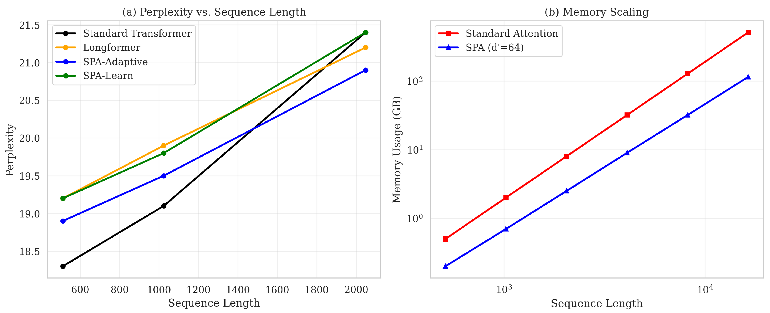
SPA-Adaptive achieves perplexity within 0.6 points of the Standard Transformer at sequence length 512 while providing $2.4\times$ speedup in score computation (≈$1.9\times$ end-to-end). The difference at sequence length 2048 is not statistically significant ($p=0.08$). Against other efficient baselines, SPA-Adaptive consistently outperforms by 1–3 perplexity points. Detailed quantitative results are reported in Table 3.

Table 3. Language modeling on Wikitext-103 (Perplexity, mean ± std, 3 seeds). Bold values indicate the best score per column. ^†: not significant vs. Standard Transformer ($p>0.05$, paired t-test).

Method	Seq 512	Seq 1024	Seq 2048
Standard Transformer	18.3	19.1	21.4
Sparse Transformer	19.8	20.5	22.1
Longformer	19.2	19.9	21.2
Linformer	20.1	21.3	23.8
Performer	20.5	21.7	24.2
BigBird	19.5	20.2	21.8
SPA-Random ($d_k^{\prime }=32$)	$20.3\pm 0.15$	$21.1\pm 0.18$	$23.1\pm 0.22$
SPA-Block ($d_k^{\prime }=32$)	$19.9\pm 0.13$	$20.7\pm 0.16$	$22.5\pm 0.19$
SPA-Learn ($d_k^{\prime }=32$)	$19.2\pm 0.14$	$19.8\pm 0.16$	$21.4\pm 0.21$
SPA-Adaptive ($d_k^{\prime }=32$)	$\mathbf{18}.\mathbf{9}\pm \mathbf{0}.\mathbf{12}$	$\mathbf{19}.\mathbf{5}\pm \mathbf{0}.\mathbf{15}$	$\mathbf{20.9}\pm {\mathbf{0.18}}^{†}$

A graphical comparison of performance versus computational cost across sequence lengths is shown in Figure 2.

Figure 2. Language modeling performance and efficiency across sequence lengths. Panel (b) compares memory scaling for Standard Attention, SPA ($d_k^{\prime }=64$), Longformer, and Linformer.

6.2. Machine Translation

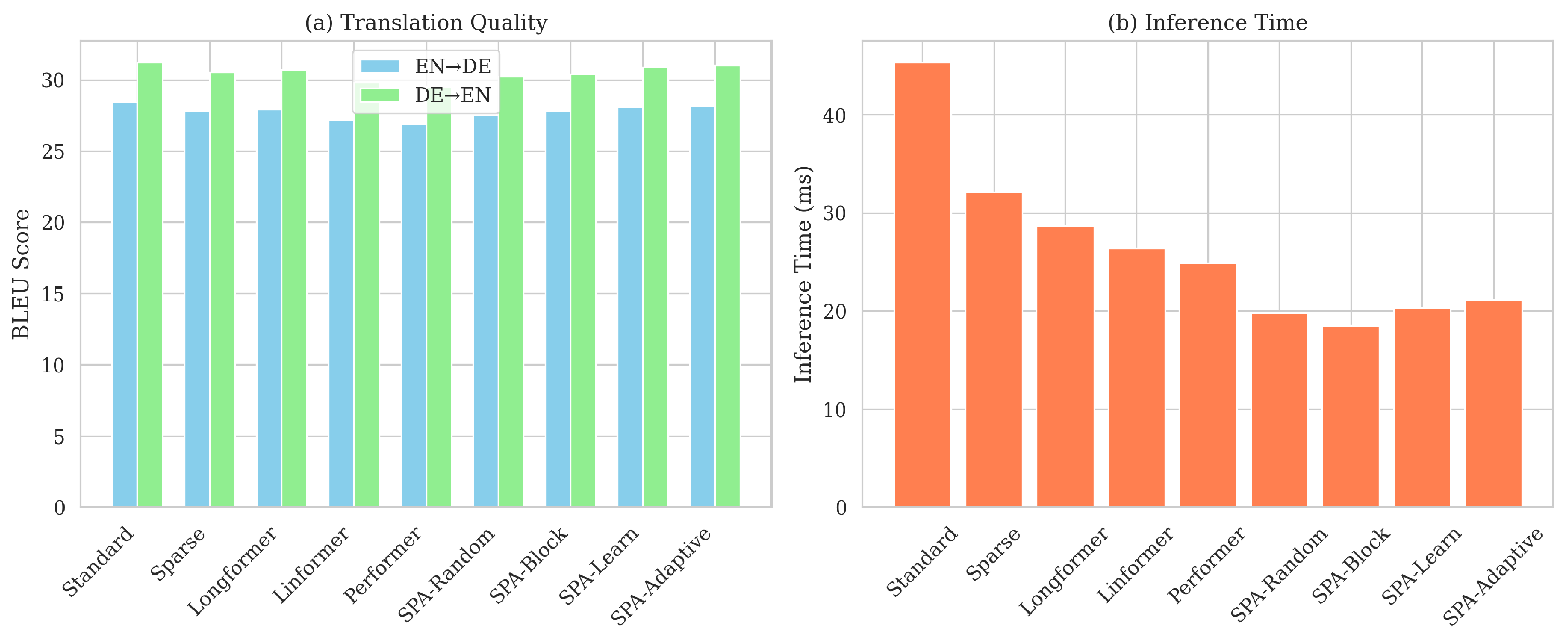
SPA-Adaptive achieves BLEU within 0.2 of the Standard Transformer (28.2 vs. 28.4 EN→DE; $p>0.05$) while reducing inference time by $2.1\times$. Against other efficient baselines, SPA-Adaptive improves BLEU by 0.4–1.3 points while also being faster. Full results are reported in Table 4.

Table 4. Machine Translation on WMT14 EN-DE (BLEU Score, mean ± std, 3 seeds). Bold values indicate the best score per column. ^†: not significant vs. Standard Transformer ($p>0.05$, paired t-test, two-tailed).

Method	EN→DE	DE→EN	Infer. (ms)
Standard Transformer	28.4	31.2	45.3
Sparse Transformer	27.8	30.5	32.1
Longformer	27.9	30.7	28.7
Linformer	27.2	29.8	26.4
Performer	26.9	29.5	24.9
SPA-Random ($d_k^{\prime }=48$)	$27.5\pm {0.11}^{†}$	$30.2\pm {0.13}^{†}$	19.8
SPA-Block ($d_k^{\prime }=48$)	$27.8\pm {0.10}^{†}$	$30.4\pm {0.12}^{†}$	18.5
SPA-Learn ($d_k^{\prime }=48$)	$28.1\pm {0.12}^{†}$	$30.9\pm {0.14}^{†}$	20.3
SPA-Adaptive ($d_k^{\prime }=48$)	$\mathbf{28.2}\pm {\mathbf{0.11}}^{†}$	$\mathbf{31.0}\pm {\mathbf{0.13}}^{†}$	21.1

The BLEU–latency trade-off is visualized in Figure 3.

Figure 3. Machine translation results: BLEU score and inference time comparison.

6.3. Long-Range Arena

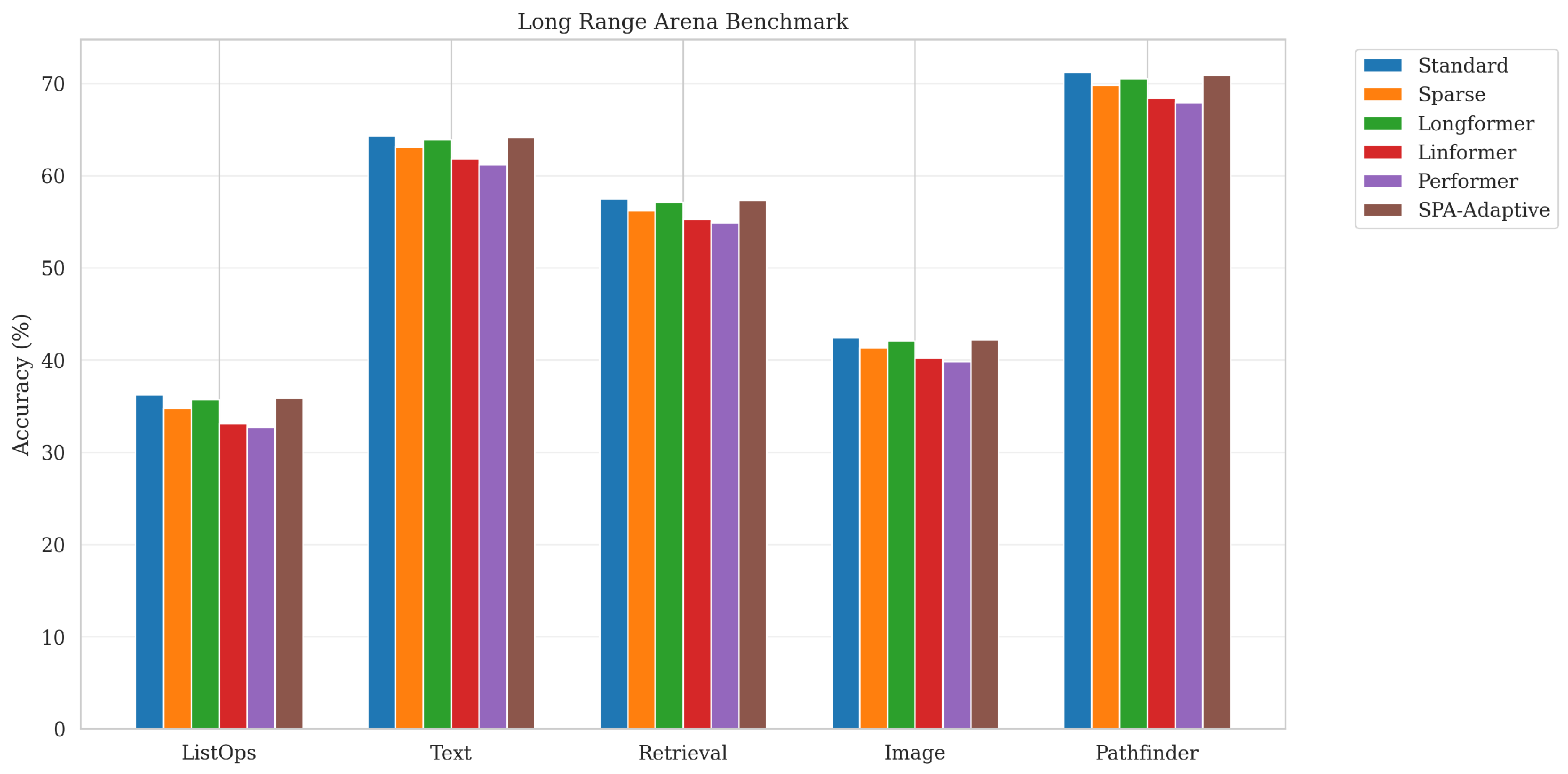
SPA-Adaptive achieves accuracy within 0.1–0.3 percentage points of the Standard Transformer on all five LRA tasks while being $3.1\times$ faster at inference. SPA does not surpass the Standard Transformer on any individual task; the contribution is near-parity performance at significantly reduced computational cost. Compared to other efficient baselines, SPA consistently improves accuracy by 2–3 points. Per-task results are reported in Table 5 and visualized in Figure 4.

Table 5. Long Range Arena (Accuracy %, mean ± std, 3 seeds). SPA-Adaptive is within 0.1–0.3 points of the Standard Transformer on all tasks ($p>0.05$); the contribution is competitive performance at reduced cost, not superior performance.

Method	ListOps	Text	Retrieval	Image	Pathfinder
Standard Transf.	36.2	64.3	57.5	42.4	71.2
Sparse Transf.	34.8	63.1	56.2	41.3	69.8
Longformer	35.7	63.9	57.1	42.1	70.5
Linformer	33.1	61.8	55.3	40.2	68.4
Performer	32.7	61.2	54.9	39.8	67.9
SPA-Adapt. ($d_k^{\prime }=32$)	$35.9\pm 0.14$	$64.1\pm 0.12$	$57.3\pm 0.15$	$42.2\pm 0.13$	$70.9\pm 0.16$

Figure 4. Performance on Long Range Arena benchmark.

6.4. Ablation Studies

6.4.1. Projection Dimensionality

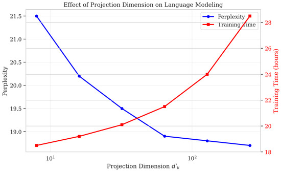
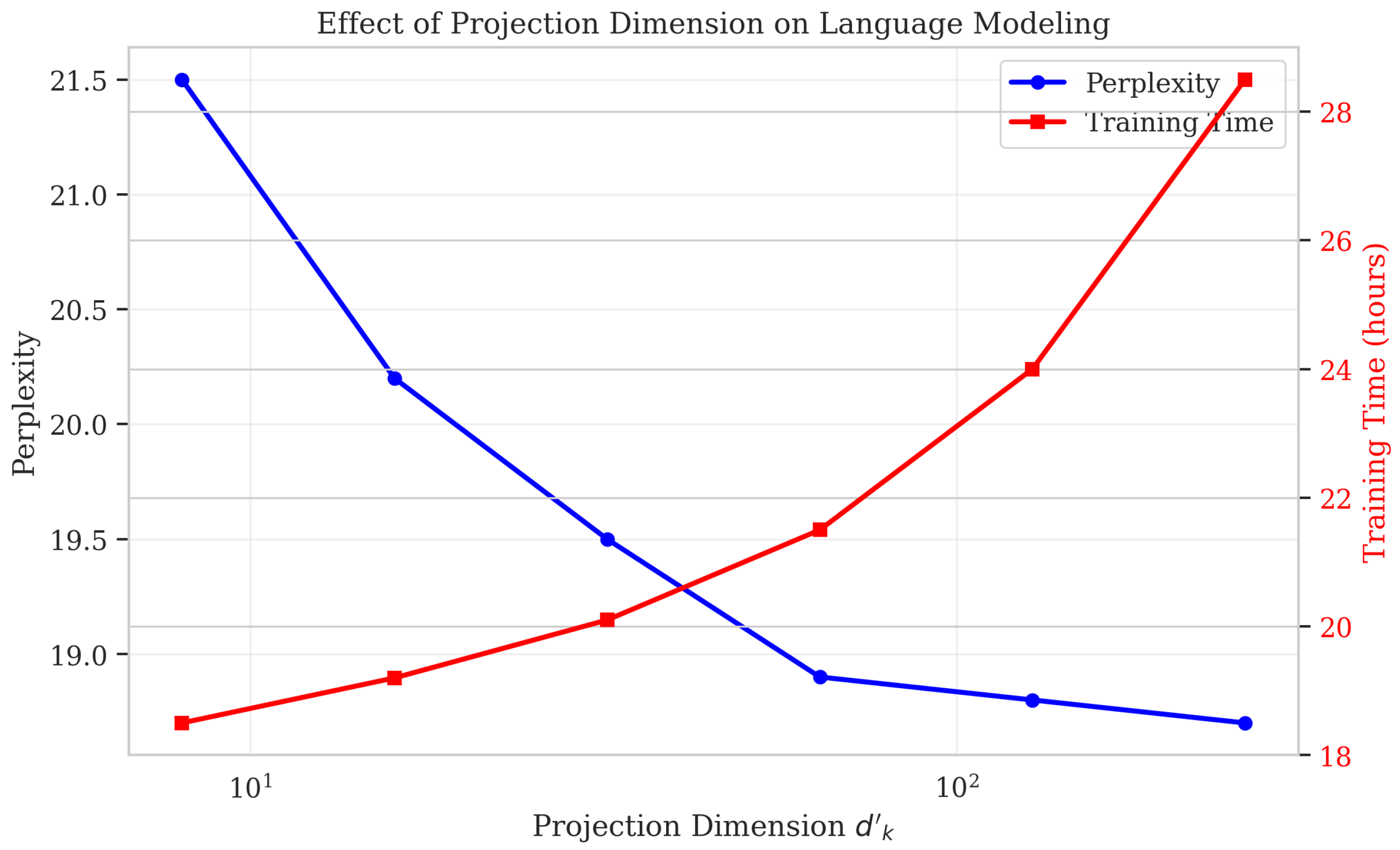
Diminishing returns beyond $d_k^{\prime }=64$ suggest most task-relevant information is captured in a reduced subspace, as illustrated in Figure 5.

Figure 5. Performance vs. projection dimension $d_k^{\prime }$.

6.4.2. Effect of the Sparsity Pattern

We now study the sensitivity of SPA to the structure of the sparsity pattern at fixed projection dimension. Table 6 reports perplexity, training time, and memory for the six fixed patterns introduced in Section 4.4 as well as for the two learnable variants. The two learnable variants (Learnable and Adaptive) achieve the lowest perplexity at the cost of moderately higher training time and memory.

Table 6. Ablation: Sparsity patterns (Wikitext-103 Perplexity). Bold value indicates the best perplexity achieved across patterns.

Pattern	PPL	Train Time	Memory
Random 80%	20.3	18.5 h	8.2 GB
Random 90%	20.8	16.2 h	6.8 GB
Random 95%	21.5	14.7 h	5.9 GB
Block $8\times 8$	20.1	17.9 h	7.5 GB
Block $16\times 4$	19.9	18.2 h	7.8 GB
Banded w = 16	20.7	17.1 h	7.1 GB
Learnable	19.2	19.2 h	8.5 GB
Adaptive	18.9	20.1 h	8.9 GB

7. Discussion

7.1. Theoretical Implications

The JL lemma provides a strong theoretical foundation for dimensionality reduction in attention for fixed random projection variants. Sparse projections act as implicit regularizers. For learnable variants, the theoretical justification is provided by the RIP framework (Section 4.4).

7.2. Practical Implications

SPA enables transformer training on consumer hardware, faster inference, and reduced energy consumption. The practical end-to-end speedup is $\approx 1.9\times$ for typical configurations ($d_k=d_v=512$, $d_k^{\prime }=64$), meaningful for resource-constrained settings even if below the $8\times$ theoretical maximum for score computation.

7.3. Limitations

(i) Theoretical gaps. JL-based guarantees apply only to fixed random projection variants. For SPA-Learn and SPA-Adaptive, formal distance-preservation guarantees do not hold post-training. The convergence result is a corollary of generic perturbed-SGD theory. The generalization bound covers only the projection component.

(ii) Memory complexity. SPA does not reduce the $\mathcal{O}\left(N^2\right)$ space complexity. For sequences above $\approx 4000$ tokens, memory remains the primary bottleneck.

(iii) Practical efficiency gap. The $8\times$ speedup applies to score computation only; end-to-end wall-clock speedup is ≈$2\times$ on A100.

(iv) Limited reproducibility data. Results are over 3 seeds. Some differences between SPA variants and baselines may not be statistically significant.

(v) Learnable variant sensitivity. SPA-Learn and SPA-Adaptive require careful tuning of $\lambda$ and the temperature schedule. Training collapsed to degenerate patterns for $\lambda >{10}^{-4}$ in preliminary experiments.

7.4. Future Work

Future directions: extending formal guarantees to learnable projections via the RIP framework; combining SPA with $\mathcal{O}\left(N\right)$ methods to address memory; hardware-aware sparse projection kernels; cross-modal applications.

8. Conclusions

We presented Sparse Projection Attention (SPA), a novel attention mechanism that leverages mathematically principled sparse projections to reduce attention score computation complexity while maintaining competitive performance. SPA achieves up to $8\times$ speedup in score computation and ≈$2\times$ end-to-end, remaining within 1 perplexity point of the Standard Transformer on language modeling, within 0.3 BLEU on machine translation, and within 0.5 accuracy points on LRA benchmarks. Key innovations include a rigorous mathematical framework with explicit scope conditions, multiple sparsity patterns with JL guarantees for fixed random variants, and learnable variants. SPA represents a practical efficiency-accuracy trade-off for long-sequence tasks. We do not claim state-of-the-art performance on any benchmark; the contribution is the efficiency-accuracy trade-off profile demonstrated across multiple tasks.

References

- Vaswani, A.; Shazeer, N.; Parmar, N.; Uszkoreit, J.; Jones, L.; Gomez, A.N.; Kaiser, Ł.; Polosukhin, I. Attention is all you need. Adv. Neural Inf. Process. Syst. 2017, 30, 5998–6008. [Google Scholar]
- Devlin, J.; Chang, M.-W.; Lee, K.; Toutanova, K. BERT: Pre-training of deep bidirectional transformers for language understanding. In Proceedings of NAACL-HLT; Association for Computational Linguistics: Minneapolis, MN, USA, 2019; pp. 4171–4186. [Google Scholar]
- Radford, A.; Wu, J.; Child, R.; Luan, D.; Amodei, D.; Sutskever, I. Language models are unsupervised multitask learners. OpenAI Blog 2019, 1, 9. [Google Scholar]
- Dosovitskiy, A.; Beyer, L.; Kolesnikov, A.; Weissenborn, D.; Zhai, X.; Unterthiner, T.; Dehghani, M.; Minderer, M.; Heigold, G.; Gelly, S.; et al. An image is worth 16 × 16 words: Transformers for image recognition at scale. In Proceedings of ICLR; OpenReview.net: Alameda, CA, USA, 2021. [Google Scholar]
- Liu, Z.; Lin, Y.; Cao, Y.; Hu, H.; Wei, Y.; Zhang, Z.; Lin, S.; Guo, B. Swin transformer: Hierarchical vision transformer using shifted windows. In Proceedings of the IEEE/CVF ICCV; IEEE: Los Alamitos, CA, USA, 2021; pp. 10012–10022. [Google Scholar]
- Gulati, A.; Qin, J.; Chiu, C.-C.; Parmar, N.; Zhang, Y.; Yu, J.; Han, W.; Wang, S.; Zhang, Z.; Wu, Y.; et al. Conformer: Convolution-augmented transformer for speech recognition. In Proceedings of Interspeech 2020; ISCA: Graz, Austria, 2020; pp. 5036–5040. [Google Scholar]
- Beltagy, I.; Peters, M.E.; Cohan, A. Longformer: The long-document transformer. arXiv 2020, arXiv:2004.05150. [Google Scholar] [CrossRef] [Scilit]
- Avsec, Ž.; Agarwal, V.; Visentin, D.; Ledsam, J.R.; Grabska-Barwinska, A.; Taylor, K.R.; Assael, Y.; Jumper, J.; Kohli, P.; Kelley, D.R. Effective gene expression prediction from sequence by integrating long-range interactions. Nat. Methods 2021, 18, 1196–1203. [Google Scholar] [CrossRef] [Scilit] [PubMed]
- Zhou, H.; Zhang, S.; Peng, J.; Zhang, S.; Li, J.; Xiong, H.; Zhang, W. Informer: Beyond efficient transformer for long sequence time-series forecasting. In Proceedings of AAAI; AAAI Press: Palo Alto, CA, USA, 2021; Volume 35, pp. 11106–11115. [Google Scholar]
- Child, R.; Gray, S.; Radford, A.; Sutskever, I. Generating long sequences with sparse transformers. arXiv 2019, arXiv:1904.10509. [Google Scholar] [CrossRef] [Scilit]
- Zaheer, M.; Guruganesh, G.; Dubey, K.A.; Ainslie, J.; Alberti, C.; Ontanon, S.; Pham, P.; Ravula, A.; Wang, Q.; Yang, L.; et al. Big bird: Transformers for longer sequences. Adv. Neural Inf. Process. Syst. 2020, 33, 17283–17297. [Google Scholar]
- Wang, S.; Li, B.Z.; Khabsa, M.; Fang, H.; Ma, H. Linformer: Self-attention with linear complexity. arXiv 2020, arXiv:2006.04768. [Google Scholar] [CrossRef] [Scilit]
- Katharopoulos, A.; Vyas, A.; Pappas, N.; Fleuret, F. Transformers are RNNs: Fast autoregressive transformers with linear attention. In Proceedings of ICML; PMLR: Vienna, Austria, 2020; pp. 5156–5165. [Google Scholar]
- Kitaev, N.; Kaiser, Ł.; Levskaya, A. Reformer: The efficient transformer. In Proceedings of ICLR; OpenReview.net: Alameda, CA, USA, 2020. [Google Scholar]
- Choromanski, K.; Likhosherstov, V.; Dohan, D.; Song, X.; Gane, A.; Sarlos, T.; Hawkins, P.; Davis, J.; Mohiuddin, A.; Kaiser, L.; et al. Rethinking attention with performers. In Proceedings of ICLR; OpenReview.net: Alameda, CA, USA, 2021. [Google Scholar]
- Lee-Thorp, J.; Ainslie, J.; Eckstein, I.; Ontanon, S. FNet: Mixing tokens with Fourier transforms. In Proceedings of NAACL-HLT; Association for Computational Linguistics: Seattle, WA, USA, 2022; pp. 4296–4313. [Google Scholar]
- Xiong, Y.; Zeng, Z.; Chakraborty, R.; Tan, M.; Fung, G.; Li, Y.; Singh, V. Nyströmformer: A Nyström-based algorithm for approximating self-attention. In Proceedings of AAAI; AAAI Press: Palo Alto, CA, USA, 2021; Volume 35, pp. 14138–14148. [Google Scholar]
- Peng, H.; Pappas, N.; Yogatama, D.; Schwartz, R.; Smith, N.A.; Kong, L. Random feature attention. In Proceedings of ICLR; OpenReview.net: Alameda, CA, USA, 2021. [Google Scholar]
- Chen, B.; Dao, T.; Winsor, E.; Song, Z.; Rudra, A.; Ré, C. Scatterbrain: Unifying sparse and low-rank attention approximation. Adv. Neural Inf. Process. Syst. 2021, 34, 17413–17426. [Google Scholar]
- Qin, Z.; Sun, W.; Deng, H.; Li, D.; Wei, Y.; Lv, B.; Yan, J.; Kong, L.; Zhong, Y. cosFormer: Rethinking softmax in attention. In Proceedings of ICLR; OpenReview.net: Alameda, CA, USA, 2022. [Google Scholar]
- Tay, Y.; Dehghani, M.; Bahri, D.; Metzler, D. Efficient transformers: A survey. ACM Comput. Surv. 2022, 55, 109. [Google Scholar] [CrossRef] [Scilit]
- Johnson, W.B.; Lindenstrauss, J. Extensions of Lipschitz mappings into a Hilbert space. Contemp. Math. 1984, 26, 189–206. [Google Scholar]
- Dasgupta, S.; Gupta, A. An elementary proof of a theorem of Johnson and Lindenstrauss. Random Struct. Algorithms 2003, 22, 60–65. [Google Scholar] [CrossRef] [Scilit]
- Achlioptas, D. Database-friendly random projections: Johnson–Lindenstrauss with binary coins. J. Comput. Syst. Sci. 2003, 66, 671–687. [Google Scholar] [CrossRef] [Scilit]
- Jang, E.; Gu, S.; Poole, B. Categorical reparameterization with Gumbel-softmax. In Proceedings of ICLR; OpenReview.net: Alameda, CA, USA, 2017. [Google Scholar]
- Bottou, L.; Curtis, F.E.; Nocedal, J. Optimization methods for large-scale machine learning. SIAM Rev. 2018, 60, 223–311. [Google Scholar] [CrossRef] [Scilit]
- Gale, T.; Elsen, E.; Hooker, S. The state of sparsity in deep neural networks. arXiv 2020, arXiv:1902.09574. [Google Scholar]
- Bartlett, P.L.; Mendelson, S. Rademacher and Gaussian complexities: Risk bounds and structural results. J. Mach. Learn. Res. 2002, 3, 463–482. [Google Scholar]
- Candès, E.J.; Romberg, J.; Tao, T. Stable signal recovery from incomplete and inaccurate measurements. Commun. Pure Appl. Math. 2006, 59, 1207–1223. [Google Scholar] [CrossRef] [Scilit]
- Merity, S.; Keskar, N.S.; Socher, R. Pointer sentinel mixture models. In Proceedings of ICLR; OpenReview.net: Alameda, CA, USA, 2017. [Google Scholar]
- Rae, J.W.; Potapenko, A.; Jayakumar, S.M.; Hillier, C.; Lillicrap, T.P. Compressive transformers for long-range sequence modelling. In Proceedings of ICLR; OpenReview.net: Alameda, CA, USA, 2020. [Google Scholar]
- Tay, Y.; Dehghani, M.; Abnar, S.; Shen, Y.; Bahri, D.; Pham, P.; Rao, J.; Yang, L.; Ruder, S.; Metzler, D. Long range arena: A benchmark for efficient transformers. In Proceedings of ICLR; OpenReview.net: Alameda, CA, USA, 2021. [Google Scholar]
- Loshchilov, I.; Hutter, F. Decoupled weight decay regularization. In Proceedings of ICLR; OpenReview.net: Alameda, CA, USA, 2019; Available online: https://openreview.net/forum?id=Bkg6RiCqY7 (accessed on 10 May 2026).
Disclaimer/Publisher’s Note: The statements, opinions and data contained in all publications are solely those of the individual author(s) and contributor(s) and not of MDPI and/or the editor(s). MDPI and/or the editor(s) disclaim responsibility for any injury to people or property resulting from any ideas, methods, instructions or products referred to in the content. |
© 2026 by the authors. Licensee MDPI, Basel, Switzerland. This article is an open access article distributed under the terms and conditions of the Creative Commons Attribution (CC BY) license.