Modeling Foot-and-Mouth Disease Dynamics Among Livestock and Wild Ruminants: Integrating Community Viral Load and Environmental Transmission Pathways

Abstract

Foot-and-mouth disease (FMD) is a highly transmissible viral infection of livestock that threatens food security and causes substantial economic losses in endemic regions. Despite its economic impact, the role of environmental viral load and wildlife reservoirs in sustaining FMD transmission remains poorly quantified. The aim of this study is to assess the extent to which community viral load sustains FMD persistence and to identify key transmission drivers in a coupled livestock–wildlife–environment system. A Susceptible–Exposed–Infected (SEI) model with a free-living virus compartment was analyzed via the basic reproduction number ($R_0$) and solved numerically using a Nonstandard Finite Difference Method. Sensitivity analysis identified wild host population size, transmission rates, host recruitment, environmental viral decay, and viral load thresholds as major determinants of $R_0$. Results indicate that higher transmission rates accelerate susceptible depletion and increase exposed and infected classes, with wildlife dominating environmental viral contributions. Community viral load is central to sustaining outbreaks and informs targeted control strategies.

1. Introduction

Livestock diseases pose a significant threat to global food security, poverty reduction, and economic development [1,2,3,4,5,6,7]. Among these, foot-and-mouth disease (FMD) is one of the most economically devastating due to its highly contagious nature and broad host range, affecting cattle, pigs, sheep, and goats [8]. The disease is characterized by fever and vesicular lesions in the mouth and on the feet of infected animals, resulting in reduced productivity, weight loss, and severe trade restrictions [9,10]. Although mortality in adult animals is generally low, young animals may experience myocarditis and sudden death, while dairy cattle suffer substantial losses in milk production and pigs exhibit reduced growth rates [8,11]. FMD is caused by an RNA virus of the genus Aphthovirus (family Picornaviridae) and exists in seven immunologically distinct serotypes (O, A, C, Asia1, SAT1, SAT2, SAT3), with no cross-protection between them [12,13]. This antigenic diversity complicates vaccination and long-term disease control. Consequently, outbreaks lead to major economic losses due to culling, trade bans, and movement restrictions [10]. While FMD has been eradicated from most high-income countries, it remains endemic in many parts of Asia, Africa, and South America, where limited resources, inadequate surveillance systems, and the presence of wildlife reservoirs hinder effective control [13]. Mathematical and computational models have played a crucial role in understanding FMD transmission dynamics, informing risk assessment, and evaluating control strategies [14,15,16]. Following the 2001 United Kingdom foot-and-mouth disease outbreak, a substantial body of modeling work was developed to study epidemic spread [17]. However, most of these models were designed for non-endemic, high-income settings and primarily focus on the post-detection phase, where local transmission between farms or herds is the dominant driver of infection [18,19,20]. In contrast, FMD persistence in endemic regions is driven by more complex processes, including waning immunity, repeated viral introductions, and cross-species transmission involving wildlife reservoirs [21]. These differences limit the applicability of existing models, as variations in farming systems, animal movement patterns, and ecological conditions significantly influence disease dynamics.

A wide range of modeling approaches has been developed to study FMD, including stochastic farm-level simulations, network-based models, and optimization frameworks for vaccination and resource allocation [14,15,16]. For example, Belsham [22] investigated transmission rates associated with carrier animals, while Kao et al. [23] developed a network-based framework to analyze epidemic spread. Other studies have examined the effectiveness of combined control strategies, such as vaccination and culling, demonstrating that integrated approaches can reduce transmission when sufficient resources are available [24]. More recent work has extended these frameworks to near-endemic settings, highlighting the importance of sustained vaccination strategies for long-term control. Despite these advances, many existing models emphasize direct host-to-host transmission and often neglect the role of environmental viral persistence and wildlife reservoirs in sustaining infection. In endemic regions, disease persistence is influenced by a combination of factors, including reinfection, multi-host interactions, and environmental contamination, all of which are difficult to quantify due to limited data availability [10,25]. The coexistence of domestic livestock and wild ruminants further complicates control efforts, as these populations differ in susceptibility, contact structure, and transmission potential [26]. Consequently, traditional control measures such as vaccination, culling, and movement restrictions remain insufficient in many settings. Infectious disease systems are inherently complex, involving interactions among the host, pathogen, and environment [27]. The environment, in particular, can act both as a reservoir of infectious agents and as a medium facilitating transmission between hosts. In the context of FMD, the virus can survive outside the host for extended periods, enabling indirect transmission through contaminated environments and interactions between domestic and wild animal populations. However, the contribution of community viral load to disease persistence remains insufficiently understood. To address this gap, this study develops and analyzes a mathematical model of FMD transmission within a coupled livestock–wildlife–environment system. The model incorporates susceptible, exposed, and infected compartments for both domestic and wild ruminants, together with an environmental viral load compartment representing the accumulation and decay of infectious viral particles. Environmental contamination arises from viral shedding by infected animals, while feedback mechanisms allow for reinfection of susceptible hosts. By integrating both direct transmission and indirect transmission mediated through environmental viral persistence, the model provides a more realistic representation of FMD dynamics in endemic settings. The aim of this study is to develop a novel epidemiological framework that explicitly incorporates community viral load into a multi-host transmission system. It examines the extent to which community viral load can sustain the persistence of foot-and-mouth disease and identifies the key parameters driving its transmission dynamics. Additionally, it provides a foundation for understanding the roles of wildlife reservoirs and environmental contamination in long-term disease persistence, and for evaluating the effectiveness of targeted control interventions. Accordingly, this study addresses the following research question: How do interactions among livestock, wildlife, and the environment including environmental viral load shape the transmission dynamics and persistence of foot-and-mouth disease, and what insights can these dynamics provide for the design of effective disease control strategies in endemic settings?

The remainder of this paper is organized as follows. Section 2 presents the development of the foot-and-mouth disease transmission model system. Mathematical analysis of the foot-and-mouth disease transmission model system is performed in Section 3. In Section 4, we present the sensitivity analysis of the foot-and-mouth disease transmission model system. Section 5 describes the construction of the Nonstandard Finite Difference (NSFD) scheme and the corresponding numerical analysis of the model. Finally, Section 6 provides the discussion and conclusions.

2. Model Formulation and Mathematical Analysis

In this section, we formulate and examine an epidemiological model for foot-and-mouth disease (FMD). The model captures the transmission dynamics of FMD among wild and domestic animal populations, driven by both direct and indirect contact with the virus (FMDV). It tracks the evolution of eight distinct compartments over time t, denoted as follows: susceptible wild animals $S_W\left(t\right)$, susceptible domestic animal $S_D\left(t\right)$, exposed wild animals $E_W\left(t\right)$, exposed domestic animal $E_D\left(t\right)$, infected wild animal $I_W\left(t\right)$, infected domestic animal $I_D\left(t\right)$ and community/regional FMDV load $V_E\left(t\right)$. We made the following assumptions for the FMD model:

(i)

The disease is not transmitted vertically.

(ii)

The total populations of both domestic and wild animals are assumed to remain constant.

(iii)

Disease transmission occurs through contact with the community viral load $\left(V_E\right)$, which represents both direct and indirect pathways of infection.

(v)

The community viral load $V_E$ = $V_E\left(t\right)$ serves as a proxy for the infectiousness of both domestic and wild ruminants and is assumed to be shed via feces by infected individuals.

(vi)

Domestic and wild animals enter their respective populations through birth.

A summary of the model variables along with the model parameters is given in Table 1 and Table 2, respectively.

Table 1. Description of variables in the model (1).

Variable	Variable Description
$S_D$(t)	Susceptible domestic population at time (t)
$E_D\left(t\right)$	Exposed domestic population at time (t)
$I_D$(t)	Infected domestic population at time (t)
$S_W$(t)	Susceptible wild population at time (t)
$E_W$(t)	Exposed wild population at time (t)
$I_W$(t)	Infected wild population at time (t)
$V_E$(t)	FMD Viral load at time (t)
$V_0$	Viral load threshold required for infection in domestic animals
$V_1$	Viral load threshold required for infection in wild animals

Table 2. Description of parameters in the FMD transmission model, including their values, units, and references or assumptions.

Parameter	Description	Value	Reference/Note
${\beta }_D$	Transmission rate for domestic ruminants	$0.05{\mathrm{day}}^{-1}$	[28]
${\beta }_W$	Transmission rate for wild ruminants	$0.03{\mathrm{day}}^{-1}$	[28]
${\alpha }_D$	Rate at which exposed domestic ruminants become infectious	$0.1{\mathrm{day}}^{-1}$	Assumed
${\alpha }_W$	Rate at which exposed wild ruminants become infectious	$0.1{\mathrm{day}}^{-1}$	Assumed
${\mu }_D$	Natural death rate in the domestic ruminant population	$0.01{\mathrm{day}}^{-1}$	[29]
${\mu }_W$	Natural death rate in the wild ruminant population	$0.01{\mathrm{day}}^{-1}$	[29]
${\delta }_D$	Disease-induced death rate in the domestic ruminant population	$0.05{\mathrm{day}}^{-1}$	[30]
${\delta }_W$	Disease-induced death rate in the wild ruminant population	$0.05{\mathrm{day}}^{-1}$	[30]
${\Lambda }_D$	Birth rate in the domestic ruminant population	$0.3{\mathrm{day}}^{-1}$	[31]
${\Lambda }_W$	Birth rate in the wild ruminant population	$0.4{\mathrm{day}}^{-1}$	[31]
$N_d$	Average FMD community viral load due to domestic animals	100 viral load units	Assumed
$N_w$	Average FMD community viral load due to wild animals	100 viral load units	Assumed
${\alpha }_V$	FMD viral load decay rate in the environment	$0.01{\mathrm{day}}^{-1}$	Assumed
${\alpha }_d$	Excretion rate of FMD viral load by infected domestic animals	$0.02{\mathrm{day}}^{-1}$	Assumed
${\alpha }_w$	Excretion rate of FMD viral load by infected wild animals	$0.02{\mathrm{day}}^{-1}$	Assumed
$V_0$	FMD viral load threshold for domestic infection	100 viral load units	Assumed
$V_1$	FMD viral load threshold for wild infection	30 viral load units	Assumed

Table 2 presents the model parameter values. In the absence of direct empirical estimates, the viral excretion parameters ${\alpha }_d$ and ${\alpha }_w$ were assigned $0.1{\mathrm{day}}^{-1}$, corresponding to an average shedding period of 10 days, consistent with experimental studies in FMD-infected cattle [32]. Other parameters, including ${\alpha }_V$, $V_0$, and $V_1$, representing environmental viral decay and viral load thresholds for domestic and wild hosts, were assumed based on biological plausibility to ensure realistic disease dynamics. Due to limited published data on FMDV, and some were chosen to ensure realistic model behavior.

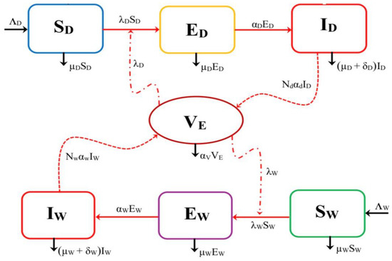
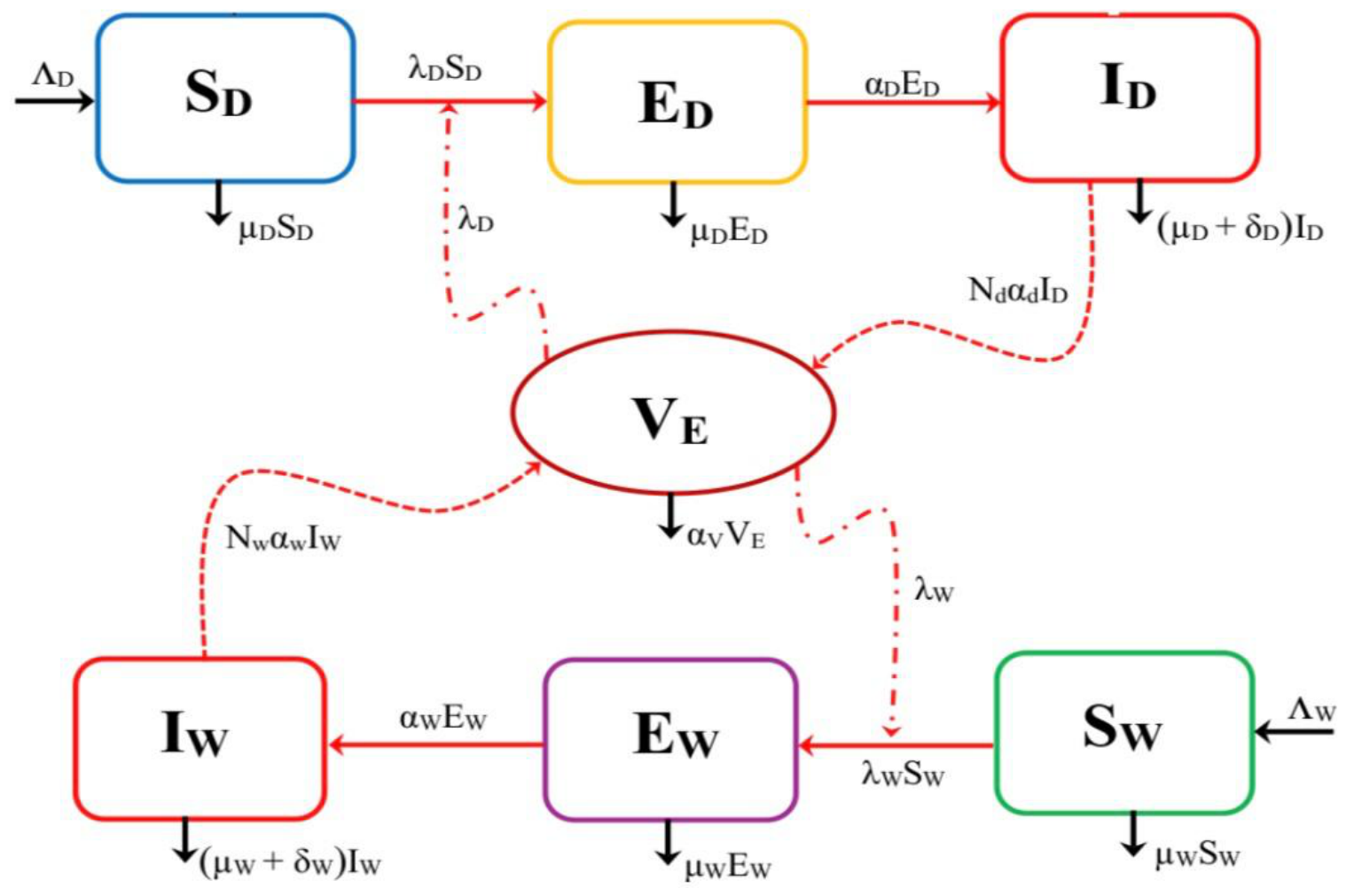
Figure 1 below presents a schematic diagram illustrating the transmission of FMD between domestic and wild animal populations.

Figure 1. A schematic illustration of the foot-and-mouth disease epidemiological model.

Based on the schematic diagram in Figure 1 and the assumptions outlined above, the complete model is described by the following system of differential equations:

$$\left\{\begin{array}{c}1.\dot{S_D}={\Lambda }_D-{\lambda }_D{S}_D-{\mu }_D{S}_D,\hfill \\ \\ 2.\dot{E_D}={\lambda }_D{S}_D-({\mu }_D+{\alpha }_D)E_D,\hfill \\ \\ 3.\dot{I_D}={\alpha }_D{E}_D-({\mu }_D+{\delta }_D)I_D,\hfill \\ \\ 4.\dot{V_E}=N_d{\alpha }_d{I}_D+N_w{\alpha }_w{I}_W-{\alpha }_V{V}_E,\hfill \\ \\ 5.\dot{S_W}={\Lambda }_W-{\lambda }_W{S}_W-{\mu }_W{S}_W,\hfill \\ \\ 6.\dot{E_W}={\lambda }_W{S}_W-({\mu }_W+{\alpha }_W)E_W,\hfill \\ \\ 7.\dot{I_W}={\alpha }_W{E}_W-({\mu }_W+{\delta }_W)I_W,\hfill \end{array}\right.$$

(1)

where ${\lambda }_W={\displaystyle \frac{{\beta }_W{V}_E{S}_W}{V_0+V_E}}$ and ${\lambda }_D={\displaystyle \frac{{\beta }_D{V}_E{S}_D}{V_1+V_E}}.$

The first equation in the model system (1) is the susceptible population at time t, which increases as new susceptible domestic animals are added to the class through births at a constant recruitment rate ${\Lambda }_D$. It is assumed that all newly recruited domestic animals are susceptible. Additionally, the number of susceptible domestic animals declines either due to infection at a rate ${\lambda }_D$ or natural death at a rate ${\mu }_D$. ${\beta }_D$ represents the transmission rate and $V_0$ indicates the FMDV saturation level. The second equation in the model system (1) represents the exposed domestic animal population $E_D\left(t\right)$; this population grows over time as susceptible animals become infected and enter this class. It is also assumed that this population declines either due to natural mortality at rate ${\mu }_D$ or progression to the infected class at a constant rate ${\alpha }_D$. The third equation in the model system (1) is the infected domestic animal population, which increases as exposed animals transition into the infected class at a rate ${\alpha }_D$. Additionally, it is assumed that this population declines due to natural mortality at rate ${\mu }_D$ and disease-related deaths at rate ${\delta }_D$. In the fourth equation of the model system (1), the dynamics of the FMDV population are represented by the average number of infectious viral particles shed into the environment by infected domestic and wild animals. Both groups contribute to environmental contamination at distinct rates: ${\alpha }_W$ denotes the rate at which each infected wild animal releases infectious FMDV particles $N_W$, while ${\alpha }_d$ represents the rate at which infected domestic animals excrete infectious FMDV particles $N_d$ into the environment. The FMDV population is assumed to decay naturally at a rate ${\alpha }_V$. In the fifth equation of the model system (1), the susceptible wild animal population at any time t increases as new individuals are added at a constant rate ${\Lambda }_W\left(t\right)$, assumed to result from natural births. All newly recruited wild animals are considered susceptible. This population declines either due to infection at a rate ${\lambda }_W$ or natural death at a rate ${\mu }_W\left(t\right)$. Here, ${\beta }_W$ denotes the transmission rate within the wild animal population, and $V_1$ represents the FMDV saturation level. The sixth equation of the model system (1) represents the exposed wild animal population, $E_W\left(t\right)$. This population increases as susceptible individuals become infected and enter this class. It is assumed to decline due to natural death at a rate ${\mu }_W$ or to progress to the infected class at a constant rate ${\alpha }_W$. The seventh equation of the model system (1) represents the infected wild animal population. This population increases as exposed wild animals transition into the infected class at a rate ${\alpha }_W$ and decreases due to natural mortality at a rate ${\mu }_W$ and disease-induced mortality at a rate ${\delta }_W$.

3. Mathematical Analysis for Foot-and-Mouth Disease Model Dynamics

In this section, we examine the mathematical properties of the model system given by Equation (1). Our primary goal is to show that all solutions remain positive. Beginning with non-negative initial conditions, we will prove that the solutions stay non-negative throughout. Furthermore, we will confirm that the model is well-posed.

3.1. Positivity

Theorem 1.

Given the initial conditions of the model system (1), $S_D\left(0\right)\ge 0, E_D\left(0\right)\ge 0$, $I_D\left(0\right)\ge 0, S_W\left(0\right)\ge 0, E_W\left(0\right)\ge 0, I_W\left(0\right)\ge 0, V_E\left(0\right)\ge 0$, the resulting solutions, $S_D\left(t\right), E_D\left(t\right), I_D\left(t\right), S_W\left(t\right), E_W\left(t\right), I_W\left(t\right), V_E\left(t\right)$, are all positive for all $t\ge$ 0.

Proof. 

Consider the first equation of the model system (1) and note that $\dot{S_D}={\displaystyle \frac{d{S}_D\left(t\right)}{dt}}$, a differential inequality governing the time evolution of the susceptible domestic animal population, is expressed as:

$${\displaystyle \frac{d{S}_D\left(t\right)}{dt}}\ge -({\mu }_D+{\lambda }_D\left(t\right))S_D\left(t\right),$$

(2)

which can be solved using the method of separation of variables, yielding:

$${\displaystyle \frac{d{S}_D\left(t\right)}{S_D\left(t\right)}}\ge -({\mu }_D+{\lambda }_D\left(t\right))dt.$$

(3)

Now, by letting

$$\widehat{t}=sup\{t>0:S_D>0;E_D>0;I_D>0;I_W>0;S_W>0;I_W>0;V_E>0\}\in [0,t],$$

and integrating Equation (3), we get

$$ln|S_D\left(t\right)|\ge -({\mu }_D\left(t\right)+{\int }_0^t{\lambda }_D\left(\widehat{t}\right)d\widehat{t})+C_1.$$

(4)

So that

$$S_D\left(t\right)\ge S_D\left(0\right).exp\{-({\mu }_D\left(t\right)+{\int }_0^t{\lambda }_D\left(\widehat{t}\right)d\widehat{t}\left)\right\}>0.$$

(5)

This implies that

$$\underset{t\to \infty }{\lim }\inf \left(S_D\left(t\right)\right)\ge 0.$$

(6)

From the second equation of the model system (1), a differential inequality representing the time dynamics of exposed domestic animals is formulated as:

$${\displaystyle \frac{d{E}_D\left(t\right)}{dt}}\ge -({\mu }_D+{\alpha }_D)E_D,$$

(7)

then integrating Equation (7), we have

$$ln|E_D\left(t\right)|\ge -({\mu }_D\left(t\right)+{\alpha }_D\left(t\right))+C_1.$$

(8)

so that

$$E_D\left(t\right)\ge E_D\left(0\right).exp\{-({\mu }_D\left(t\right)+{\alpha }_D\left(t\right)\left)\right\}>0.$$

(9)

This implies that

$$\underset{t\to \infty }{\lim }\inf \left(E_D\left(t\right)\right)\ge 0.$$

(10)

Similarly, it can be shown that solutions of $I_D>0, S_W>0, E_W>0, I_W>0$ and $V_E>0$ for all t > 0. □

3.2. Feasible Region

Letting $N_D=S_D+E_D+I_D$ and adding the 1st–3rd equations of model system (1), we obtain

$${\displaystyle \frac{d{N}_D\left(t\right)}{dt}}={\Lambda }_D-{\mu }_D{N}_D\left(t\right)-{\delta }_D{I}_D.$$

(11)

Now, assuming that

$${\displaystyle \frac{d{N}_D\left(t\right)}{dt}}\le {\Lambda }_D-{\mu }_D{N}_D\left(t\right),$$

(12)

which then implies that

$$\underset{t\to \infty }{\lim }\sup \left(N_D\left(t\right)\right)\le {\displaystyle \frac{{\Lambda }_D}{{\mu }_D}}.$$

(13)

Furthermore, concerning the wild animal population, we let $N_w=S_w+E_w+I_w$ and adding the 5th–7th equations of model system (1), we obtain

$${\displaystyle \frac{d{N}_W\left(t\right)}{dt}}={\Lambda }_W-{\mu }_W{N}_W\left(t\right)-{\delta }_W{I}_W,$$

(14)

so that

$${\displaystyle \frac{d{N}_W\left(t\right)}{dt}}\le {\Lambda }_W-{\mu }_W{N}_W\left(t\right),$$

(15)

which then implies that

$$\underset{t\to \infty }{\lim }\sup \left(N_W\left(t\right)\right)\le {\displaystyle \frac{{\Lambda }_W}{{\mu }_W}}.$$

(16)

In the same way, the fourth equation of the model system (1) can be written as

$${\displaystyle \frac{d{V}_E\left(t\right)}{dt}}=N_d{\alpha }_d{I}_D+N_w{\alpha }_w{I}_W-{\alpha }_V{V}_E,$$

(17)

and when substituting $I_D$ and $I_W$ with $N_D\left(t\right)\le {\displaystyle \frac{{\Lambda }_D}{{\mu }_D}}$ and $\left(N_W\left(t\right)\right)\le {\displaystyle \frac{{\Lambda }_W}{{\mu }_W}}$, respectively, we get:

$${\displaystyle \frac{d{V}_E\left(t\right)}{dt}}\le \left[N_d{\alpha }_d{\displaystyle \frac{{\Lambda }_D}{{\mu }_D}}+N_w{\alpha }_w{\displaystyle \frac{{\Lambda }_W}{{\mu }_W}}\right]-{\alpha }_V{V}_E,$$

(18)

Thus, the solution to Equation (18) can be found by applying an appropriate integrating factor ($e^{-{\alpha }_{E}t}$) to obtain

$$V_E\left(t\right)\le \left[{\displaystyle \frac{{\Lambda }_D{N}_d{\alpha }_d}{{\mu }_D{\alpha }_E}}+{\displaystyle \frac{{\Lambda }_W{N}_w{\alpha }_w}{{\mu }_W{\alpha }_V}}\right]+C{e}^{-{\alpha }_{E}t}.$$

(19)

This implies that

$$\underset{t\to \infty }{\lim }\sup \left(V_E\left(t\right)\right)\le \left[{\displaystyle \frac{{\Lambda }_D{N}_d{\alpha }_d}{{\mu }_D{\alpha }_V}}+{\displaystyle \frac{{\Lambda }_W{N}_w{\alpha }_w}{{\mu }_W{\alpha }_V}}\right].$$

(20)

We let

$$\left\{\begin{array}{c}\Omega =\{(S_D\left(t\right),E_D\left(t\right),I_D\left(t\right),V_E\left(t\right)),S_D\left(t\right),E_D\left(t\right),I_D\left(t\right)|0\hfill \\ \le S_D\left(t\right)+E_D\left(t\right)+I_D\left(t\right)\le Z_1,\hfill \\ 0\le S_D\left(t\right)+E_D\left(t\right)+I_D\left(t\right)\le Z_2,0\le V_E\left(t\right)\le Z_3\}.\hfill \end{array}\right.$$

(21)

be an invariant region of the model system (1), where

$$\left\{\begin{array}{c}{Z}_1={\displaystyle \frac{{\Lambda }_D}{{\mu }_D}},Z_2={\displaystyle \frac{{\Lambda }_W}{{\mu }_W}},\hfill \\ \\ Z_3=\left[{\displaystyle \frac{{\Lambda }_D{N}_d{\alpha }_d}{{\mu }_D{\alpha }_V}}+{\displaystyle \frac{{\Lambda }_W{N}_w{\alpha }_w}{{\mu }_W{\alpha }_V}}\right].\hfill \end{array}\right.$$

(22)

Therefore, $\Omega$ is a positively invariant and attracting region because every solution that begins within $\Omega$ stays there for all $t\ge 0$. Consequently, we can confidently conclude that the model system (1) is both mathematically and epidemiologically well-posed, having non-negative, bounded solutions with existence and uniqueness [33]. Hence, it suffices to analyze the dynamics of the flow generated by the model system within $\Omega$.

3.3. Disease-Free Steady State and Its Stability

The disease-free steady state (DFE) refers to the condition where all animal populations are free of foot-and-mouth disease infection. To find the DFE of the model system (1), we set $I_D=E_D=V_E=E_W=I_W=0$ and then equate the left-hand side of the system (1) to zero, resulting in:

$$\left\{\begin{array}{c}{E}_0=(S_D^0,E_D^0,I_D^0,V_E^0,S_W^0,E_W^0,I_W^0),\hfill \\ \\ E_0=({\displaystyle \frac{{\Lambda }_D}{{\mu }_D}},0,0,0,{\displaystyle \frac{{\Lambda }_W}{{\mu }_W}},0,0,).\hfill \end{array}\right.$$

(23)

Here, $E_0$ represents the disease-free equilibrium point of the model system (1) in the absence of vaccination. The basic reproduction number $R_0$ for the FMD system is calculated using the next-generation operator method. Accordingly, the model system (1) can be expressed in the following form:

$$\begin{array}{c}\hfill \left\{\begin{array}{ccc}{\displaystyle \frac{dX}{dt}}\hfill & =& f(X,Y,Z),\hfill \\ & & \\ {\displaystyle \frac{dY}{dt}}\hfill & =& g(X,Y,Z),\hfill \\ & & \\ {\displaystyle \frac{dZ}{dt}}\hfill & =& h(X,Y,Z).\hfill \end{array}\right.\end{array}$$

(24)

where

• $X=(S_D,S_W)$ includes all groups of individuals who remain uninfected.
• $Y=(E_D,I_D,E_W,I_W)$ denotes all groups of infected individuals who are not capable of transmitting the infection to others.
• $Z=\left(V_E\right)$ denotes all groups of infected individuals who can transmit the infection to others.

Now, letting

$$\begin{array}{c}\hfill E_0=({\displaystyle \frac{{\Lambda }_D}{{\mu }_D}},0,0,0,{\displaystyle \frac{{\Lambda }_W}{{\mu }_W}},0,0,).\end{array}$$

(25)

correspond to the disease-free steady state of the model (1), we can assume that:

$$\begin{array}{c}\hfill \tilde{g}(X^{*},Y)=({\tilde{g}}_1(X^{*},Y),{\tilde{g}}_2(X^{*},Y),{\tilde{g}}_3(X^{*},Y),{\tilde{g}}_4(X^{*},Y)),\end{array}$$

(26)

with

$$\begin{array}{c}\hfill \left\{\begin{array}{c}{\tilde{g}}_1(X^{*},Y)={\displaystyle \frac{{\beta }_D{V}_E{\Lambda }_D}{(V_0+V_E)({\mu }_D+{\alpha }_D){\mu }_D}},\hfill \\ \\ {\tilde{g}}_2(X^{*},Y)={\displaystyle \frac{{\alpha }_D{\beta }_D{V}_E{\Lambda }_D}{(V_0+V_E)({\mu }_D+{\alpha }_D)({\mu }_D+{\delta }_D){\mu }_D}},\hfill \\ \\ {\tilde{g}}_3(X^{*},Y)={\displaystyle \frac{{\beta }_D{V}_E{\Lambda }_W}{(V_1+V_E)({\mu }_W+{\alpha }_W){\mu }_W}},\hfill \\ \\ {\tilde{g}}_4(X^{*},Y)={\displaystyle \frac{{\alpha }_W{\beta }_W{V}_E{\Lambda }_W}{(V_1+V_E)({\mu }_W+{\alpha }_W)({\mu }_W+{\delta }_W){\mu }_W}}.\hfill \end{array}\right.\end{array}$$

(27)

So that

$$\begin{array}{c}\hfill \left\{\begin{array}{ccc}{\displaystyle \frac{d{V}_E}{dt}}\hfill & =& {\displaystyle \frac{N_d{\alpha }_d{\beta }_D{\Lambda }_D}{({\mu }_D+{\alpha }_D)({\mu }_D+{\delta }_D){\mu }_D}}{\displaystyle \frac{V_E}{(V_0+V_E)}}\hfill \\ & & +{\displaystyle \frac{N_w{\alpha }_w{\beta }_W{\Lambda }_W}{({\mu }_W+{\alpha }_W)({\mu }_W+{\delta }_W){\mu }_W}}{\displaystyle \frac{V_E}{(V_1+V_E)}}-{\alpha }_V{V}_E,\hfill \\ & =& {\displaystyle \frac{a_0{V}_E}{V_0+V_E}}+{\displaystyle \frac{a_1{V}_E}{V_1+V_E}}-{\alpha }_V{V}_E.\hfill \end{array}\right.\end{array}$$

(28)

where

$$\begin{array}{c}\hfill \left\{\begin{array}{ccc}{a}_0\hfill & =& {\displaystyle \frac{N_d{\alpha }_d{\beta }_D{\Lambda }_D}{({\mu }_D+{\alpha }_D)({\mu }_D+{\delta }_D){\mu }_D}},\hfill \\ a_1\hfill & =& {\displaystyle \frac{N_w{\alpha }_w{\beta }_W{\Lambda }_W}{({\mu }_W+{\alpha }_W)({\mu }_W+{\delta }_W){\mu }_W}}.\hfill \end{array}\right.\end{array}$$

(29)

so now we have

$$\begin{array}{c}\hfill \left\{\begin{array}{ccc}h\hfill & =& {\displaystyle \frac{a_0{V}_E}{V_0+V_E}}+{\displaystyle \frac{a_1{V}_E}{V_1+V_E}},\hfill \\ {\displaystyle \frac{dh}{d{V}_E}}& =& {\displaystyle \frac{a_0{V}_0}{{(V_0+V_E)}^2}}+{\displaystyle \frac{a_1{V}_1}{{(V_1+V_E)}^2}}-{\alpha }_V,\hfill \\ {\displaystyle \frac{dh\left(E_0\right)}{d{V}_E}}& =& {\displaystyle \frac{a_0}{V_0}}+{\displaystyle \frac{a_1}{V_1}}-{\alpha }_V.\hfill \end{array}\right.\end{array}$$

(30)

can be presented in the form $A=M-D$, where

$$M={\displaystyle \frac{a_0}{V_0}}+{\displaystyle \frac{a_1}{V_1}}andD={\alpha }_V.$$

Also

$$D^{-1}={\displaystyle \frac{1}{{\alpha }_V}},$$

so that

$$\begin{array}{c}\hfill M{D}^{-1}={\displaystyle \frac{a_0}{V_0{\alpha }_V}}+{\displaystyle \frac{a_1}{V_1{\alpha }_V}}.\end{array}$$

(31)

The basic reproductive number is the spectral radius (dominant eigenvalue) of the matrix $T=M{D}^{-1}$; that is

$$\begin{array}{c}\hfill R_0={\displaystyle \frac{a_0}{V_0{\alpha }_V}}+{\displaystyle \frac{a_1}{V_1{\alpha }_V}},\end{array}$$

(32)

which can be written as

$$\begin{array}{c}\hfill R_0={\displaystyle \frac{N_d{\alpha }_d{\alpha }_D{\beta }_D{\Lambda }_D}{V_0({\mu }_D+{\alpha }_D)({\mu }_D+{\delta }_D){\mu }_D{\alpha }_V}}+{\displaystyle \frac{N_W{\alpha }_w{\alpha }_w{\beta }_W{\Lambda }_W}{V_1({\mu }_W+{\alpha }_W)({\mu }_W+{\delta }_W){\mu }_W{\alpha }_V}}.\end{array}$$

(33)

3.4. Local Stability of of Disease-Free Equilibrium

To assess the local stability of the disease-free equilibrium (DFE) for the model system (1), we linearize the system’s equations to derive the Jacobian matrix and then evaluate it at the DFE

$$E_0=({\displaystyle \frac{{\Lambda }_D}{{\mu }_D}},0,0,0,{\displaystyle \frac{{\Lambda }_W}{{\mu }_W}},0,0,).$$

(34)

We obtain:

$$\begin{array}{c}\hfill J_{E_0}=\left[\begin{array}{ccccccc}-{\mu }_D& 0& 0& -{\displaystyle \frac{{\beta }_D{\Lambda }_D}{V_0{\mu }_D}}& 0& 0& 0\\ & & & & & & \\ 0& -a_0& 0& {\displaystyle \frac{{\beta }_D{\Lambda }_D}{V_0{\mu }_D}}& 0& 0& 0\\ & & & & & & \\ 0& {\alpha }_D& -a_1& 0& 0& 0& 0\\ & & & & & & \\ 0& 0& N_d{\alpha }_d& -{\alpha }_V& 0& 0& N_w{\alpha }_w\\ & & & & & & \\ 0& 0& 0& -{\displaystyle \frac{{\beta }_W{\Lambda }_W}{V_1{\mu }_W}}& -{\mu }_W& 0& 0\\ & & & & & & \\ 0& 0& 0& {\displaystyle \frac{{\beta }_W{\Lambda }_W}{V_1{\mu }_W}}& 0& -a_2& 0\\ & & & & & & \\ 0& 0& 0& 0& 0& {\alpha }_W& -a_3\end{array}\right],\end{array}$$

where

$$\begin{array}{c}\hfill \left\{\begin{array}{c}{a}_0=({\mu }_D+{\alpha }_D),\hfill \\ \\ a_1=({\mu }_D+{\delta }_D),\hfill \\ \\ a_2=({\mu }_W+{\alpha }_W),\hfill \\ \\ a_3=({\mu }_W+{\delta }_W).\hfill \end{array}\right.\end{array}$$

(35)

The stability of the DFE is analyzed by finding the eigenvalues ${\lambda }_s$ of the Jacobian matrix. The characteristic equation for these eigenvalues is expressed as:

$${\lambda }^5+{\psi }_1{\lambda }^4+{\psi }_2{\lambda }^3+{\psi }_3{\lambda }^2+{\psi }_4\lambda +{\psi }_5=0,$$

(36)

where

$$\left\{\begin{array}{c}{\varphi }_1=a_0+a_1+a_2+a_3,\hfill \\ {\varphi }_2=a_0{a}_1+a_2{a}_3+(a_0+a_1)(a_2+a_3),\hfill \\ {\varphi }_3=a_2{a}_3(a_0+a_1)+a_0{a}_1(a_2+a_3),\hfill \\ {\varphi }_4=a_0{a}_1{a}_2{a}_3.\hfill \end{array}\right.$$

(37)

To draw conclusions about the stability of the DFE, we apply the Routh–Hurwitz criteria (36) to assess the signs of the polynomial’s eigenvalues.

$$P\left(\lambda \right)={\lambda }^5+{\varphi }_1{\lambda }^4+{\varphi }_2{\lambda }^3+{\varphi }_3{\lambda }^2+{\varphi }_4\lambda +{\varphi }_5=0,$$

(38)

Consider a polynomial with real constant coefficients $a_i$ for for $i=1,2,\dots ,n$. The n Hurwitz matrices are constructed from these coefficients $a_i$ of the polynomial $P(\Lambda )$. If the determinants of all these Hurwitz matrices are positive, then all roots of $P(\Lambda )$ have negative real parts or are negative. In our case, the following matrices are defined, with their elements consisting of the coefficients (${\varphi }_S$) of the characteristic polynomial $P(\Lambda )$ given in Equation (38):

$$\begin{array}{c}\hfill H_1=\left(\begin{array}{c}{\varphi }_1\end{array}\right),H_2=\left(\begin{array}{cc}{\varphi }_1& 1\\ {\varphi }_3& {\varphi }_2\end{array}\right),\end{array}$$

(39)

and

$$\begin{array}{c}\hfill H_3=\left(\begin{array}{ccc}{\varphi }_1& 1& 0\\ {\varphi }_3& {\varphi }_2& {\varphi }_1\\ {\varphi }_5& {\varphi }_4& {\varphi }_3\end{array}\right),H_4=\left(\begin{array}{cccc}{\varphi }_1& 1& 0& 0\\ {\varphi }_3& {\varphi }_2& {\varphi }_1& 1\\ 0& {\varphi }_4& {\varphi }_3& {\varphi }_2\\ 0& 0& {\varphi }_5& {\varphi }_4\end{array}\right).\end{array}$$

(40)

Evaluating the determinant of $H_1$, we obtain

$$\begin{array}{c}\hfill \left\{\begin{array}{ccc}|H_1|\hfill & =& \left|\begin{array}{c}{\varphi }_1\end{array}\right|\hfill \\ & & \\ & =& {\varphi }_1,\hfill \end{array}\right.\end{array}$$

(41)

the determinant of $H_2$, we get

$$\begin{array}{c}\hfill \left\{\begin{array}{ccc}|H_2|\hfill & =& \left|\begin{array}{cc}{\varphi }_1& 1\\ {\varphi }_3& {\varphi }_2\end{array}\right|\hfill \\ & & \\ & =& {\varphi }_1{\varphi }_2-{\varphi }_3,\hfill \end{array}\right.\end{array}$$

(42)

the determinant of $H_3$, we obtain

$$\begin{array}{c}\hfill \left\{\begin{array}{ccc}|H_3|\hfill & =& \left|\begin{array}{ccc}{\varphi }_1& 1& 0\\ {\varphi }_3& {\varphi }_2& {\varphi }_1\\ {\varphi }_5& {\varphi }_4& {\varphi }_3\end{array}\right|\hfill \\ & & \\ & =& {\varphi }_1{\varphi }_2{\varphi }_3-{\varphi }_1^2{\varphi }_4-{\varphi }_3^2-{\varphi }_1{\varphi }_5,\hfill \end{array}\right.\end{array}$$

(43)

and the determinant of $H_4$, we obtain

$$\begin{array}{c}\hfill \left\{\begin{array}{ccc}|H_4|\hfill & =& \left|\begin{array}{cccc}{\varphi }_1& 1& 0& 0\\ {\varphi }_3& {\varphi }_2& {\varphi }_1& 1\\ 0& {\varphi }_4& {\varphi }_3& {\varphi }_2\\ 0& 0& {\varphi }_5& {\varphi }_4\end{array}\right|\hfill \\ & & \\ & =& {\varphi }_4({\varphi }_1{\varphi }_2{\varphi }_3-{\varphi }_1^2{\varphi }_4-{\varphi }_3^2).\hfill \end{array}\right.\end{array}$$

(44)

Therefore, to ensure the local stability of the disease-free equilibrium of the model system (1), the following conditions $C_1$, $C_2$, and $C_3$ must be met:

$$\begin{array}{c}\hfill \left\{\begin{array}{ccc}& & C1:{\varphi }_1,{\varphi }_2,{\varphi }_3>0,\hfill \\ & & \\ & & C2:{\varphi }_1{\varphi }_2-{\varphi }_3>0,\hfill \\ & & \\ & & C2:{\varphi }_1{\varphi }_2{\varphi }_3-{\varphi }_1^2{\varphi }_4-{\varphi }_3^2>0.\hfill \end{array}\right.\end{array}$$

(45)

From Equation (38), it becomes obvious that all the coefficients ${\varphi }_1$, ${\varphi }_2$, ${\varphi }_3$, and ${\varphi }_4$ of the polynomial $P\left(\lambda \right)$ maintain positive values whenever $R_0<1$. In addition, the determinants of all matrices $H_1$, $H_2$, $H_3$, and $H_4$ are positive if and only if $R_0<1$. Therefore, all roots of the polynomial $P(\Lambda )$ are either negative or possess negative real parts. The results are summarized in the following theorem.

Theorem 2.

The disease-free equilibrium point of the model system (1) is locally asymptotically stable if $R_0<1$.

3.5. Global Stability

We employ the next-generation operator method [34] to establish the global stability of the disease-free equilibrium (DFE) for the model system (1). Thus the system (1) can be re-written in the form

$$\left\{\begin{array}{c}{\displaystyle \frac{dX}{dt}}=F(X,Z),\hfill \\ \\ {\displaystyle \frac{dZ}{dt}}=G(X,Z),\hfill \end{array}\right.$$

(46)

where

• X = ($S_D,S_W$) represent susceptible compartment.
• Z = $(E_D,I_D,V_E,E_W,I_W)$ represent all compartments that can infect others and those who are infected but cannot infect others.

We let

$$E_0=({\displaystyle \frac{{\Lambda }_D}{{\mu }_D}},0,0,0,{\displaystyle \frac{{\Lambda }_W}{{\mu }_W}},0,0).$$

(47)

The disease-free equilibrium (DFE) of the model system (1) is denoted by Equation (47). For $X^{*}$ to be globally asymptotically stable, the following conditions (H1) and (H2) must be satisfied.

H1. 

${\displaystyle \frac{dX}{dt}}$= F(X, 0) is globally asymptotically stable (g.a.s).

H2. 

G(X,Z) = AZ − $\widehat{G}(X,Z)$, $\widehat{G}(X,Z)$≥ 0 for (X, Z) ∈${\mathbb{R}}_{+}^6$ where A = $D_{Z}G(X^{*},0)$ is an M-matrix and ${\mathbb{R}}_{+}^6$ is the region where the model makes biological sense.

In this case, we have

$$F(X,0)=\left[\begin{array}{c}{\Lambda }_D-{\mu }_D{S}_D\\ \\ {\Lambda }_W-{\mu }_W{S}_W\end{array}\right],$$

(48)

and the matrix A is given by

$$A=\left[\begin{array}{ccccccccc}-a_0& & 0& & {\displaystyle \frac{{\beta }_D{\Lambda }_D}{{\mu }_D{V}_0}}& & 0& & 0\\ & & & & & & & & \\ N_d{\alpha }_d& & 0& & -{\alpha }_V& & 0& & N_w{\alpha }_d\\ & & & & & & & & \\ 0& & 0& & {\displaystyle \frac{{\beta }_W{\Lambda }_W}{{\mu }_W{V}_1}}& & -a_2& & 0\\ & & & & & & & & \\ 0& & 0& & 0& & -{\alpha }_W& & -a_3\end{array}\right],$$

(49)

and

$$\widehat{G}(X,Z)=\left[\begin{array}{c}{\displaystyle \frac{{\beta }_D{\Lambda }_D{V}_E}{{\mu }_D{V}_0}}-{\displaystyle \frac{{\beta }_D{V}_E{S}_D}{V_0+V_E}}\\ \\ 0\\ \\ 0\\ \\ {\displaystyle \frac{{\beta }_W{\Lambda }_W{V}_E}{{\mu }_W{V}_1}}-{\displaystyle \frac{{\beta }_W{V}_E{S}_W}{V_1+V_E}}\\ \\ 0\end{array}\right].$$

(50)

Since

$${\displaystyle \frac{{\Lambda }_D}{{\mu }_D}}\ge {\displaystyle \frac{S_D}{V_0+V_E}}\mathrm{and}{\displaystyle \frac{{\Lambda }_W}{{\mu }_W}}\ge {\displaystyle \frac{S_W}{V_1+V_E}},$$

it follows that

$$\widehat{G}(X,Z)\ge 0\mathrm{for}\mathrm{all}(X,Z)\in {\mathbb{R}}_{+}^n.$$

Furthermore, the matrix associated with the linearized infected subsystem has non-negative off-diagonal elements and therefore qualifies as an M-matrix. Hence, the conditions required for the global stability theorem are satisfied. Therefore, by

Theorem 3.

The fixed point

$$E_0=(X^{*},0)=({\displaystyle \frac{{\Lambda }_D}{{\mu }_D}},0,0,0,{\displaystyle \frac{{\Lambda }_W}{{\mu }_W}},0,0,)$$

of the model system (1) is global asymptotically stable (GAS) if $R_0$≤ 1 and the assumptions (H1) and (H2) are satisfied.

3.6. Endemic Equilibrium Point

In the case of the endemic equilibrium, we assume:

$$E^{*}=(S_D^{*},E_D^{*},I_D^{*},V_E^{*},S_W^{*},E_W^{*},I_W^{*}),$$

(51)

To determine the endemic equilibrium point of the model system (1), we equate the left-hand sides of the system’s equations to zero. The corresponding expression for the number of susceptible domestic ruminants at this equilibrium is given by:

$$S_D^{*}={\displaystyle \frac{{\Lambda }_D}{{\lambda }_D^{*}+{\mu }_D}}.$$

(52)

From the expression in Equation (52), it is observed that the number of susceptible domestic ruminants at endemic equilibrium is influenced by the average duration spent in the susceptible class and the recruitment rate of new susceptibles through natural births. Additionally, this population is affected whenever susceptible domestic animals exit the class due to infection at varying rates ${\lambda }_D$ or natural death at rate ${\mu }_D$. The endemic level of exposed domestic ruminants, as described in Equation (1), is given by:

$$E_D^{*}={\displaystyle \frac{{\lambda }_D^{*}{S}_D^{*}}{{\mu }_D+{\alpha }_D}}.$$

(53)

From Equation (53), it is clear that the number of exposed domestic ruminants at the endemic equilibrium is determined by the average duration spent in the exposed class and the rate at which susceptible domestic ruminants become infected. This population is also affected when exposed individuals exit the class, either due to natural death at a constant rate ${\mu }_D$ or by progressing to the infectious class at rate ${\alpha }_D$. The corresponding endemic value of infected domestic ruminants from Equation (1) is given by:

$$I_D^{*}={\displaystyle \frac{{\alpha }_D{E}_D^{*}}{{\mu }_D+{\delta }_D}}.$$

(54)

Similarly, from Equation (54), it can be observed that the number of infected domestic ruminants at the endemic equilibrium is influenced by the average duration spent in the infected class. This population decreases as infected individuals exit the class, either due to natural death at rate ${\mu }_D$ or disease-induced mortality at rate ${\delta }_D$. Furthermore, the endemic level of the community FMDV load is provided in Equation (1) as follows:

$$V_E^{*}={\displaystyle \frac{N_d{\alpha }_d{I}_D^{*}+N_w{\alpha }_w{I}_W^{*}}{{\alpha }_V}}.$$

(55)

As shown in Equation (55), the size of the community FMDV load at endemic equilibrium is determined by the virus’s lifespan and the rate at which infected domestic and wild ruminant populations contribute to the overall infectiousness of the community or region. This contribution occurs through the shedding of FMDV into the environment, with domestic and wild infected ruminants releasing the virus at average rates of $N_d{\alpha }_d$ and $N_w{\alpha }_w$, respectively. The endemic value of the susceptible wild ruminant population is now given by:

$$S_W^{*}={\displaystyle \frac{{\Lambda }_W}{{\lambda }_W^{*}+{\mu }_W}}.$$

(56)

From Equation (56), it is noticeable that the number of susceptible wild ruminants at endemic equilibrium is influenced by the average duration spent in the susceptible class and the recruitment rate of new individuals through natural births, denoted by ${\Lambda }_W$. This population decreases as wild ruminants exit the susceptible class, either by becoming infected at a variable rate ${\lambda }_D$ and transitioning to the exposed class, or by dying naturally at a rate ${\mu }_W$. The corresponding endemic value of exposed wild ruminants, as given in Equation (1), is:

$$E_W^{*}={\displaystyle \frac{{\lambda }_W^{*}{S}_W^{*}}{{\mu }_W+{\alpha }_W}}.$$

(57)

From Equation (57), it is clear that the population of exposed wild ruminants at endemic equilibrium is determined by the average time individuals remain in the exposed class and the rate at which susceptible wild ruminants acquire infection. Additionally, individuals in this class exit either through natural death at a constant rate ${\mu }_W$ or by progressing to the infectious class at rate ${\alpha }_W$. The endemic level of infected wild ruminants, as described in Equation (1), is given by:

$$I_W^{*}={\displaystyle \frac{{\alpha }_W{E}_W^{*}}{{\mu }_W+{\delta }_W}}.$$

(58)

It can also be observed from Equation (58) that the number of infected wild ruminants at endemic equilibrium is influenced by the average duration spent in the infected class and the rate at which susceptible wild ruminants become infected. This population decreases as infected individuals exit the class due to natural death at rate ${\mu }_W$ or disease-induced mortality at rate ${\delta }_W$.

3.7. Local Stability of Endemic Equilibrium Point

To analyze the local stability of the endemic equilibrium and non-hyperbolic equilibrium points, we apply the Center Manifold Theory [35]. The theorem is presented as follows:

Theorem 4

(Center Manifold Theory). Consider the general system of ordinary differential equations involving a parameter ϕ:

(1) 

A = $D_{x}f(0,0)=\left({\displaystyle \frac{\partial f_i(0,0)}{\partial x_i}}\right)$; this is called linearization of the system at the equilibrium 0 with ϕ evaluated at 0.

(2) 

A has an eigenvalue of zero and other eigenvalues have the negative real part.

(3) 

The left eigenvector of matrix A is denoted by u and the right eigenvector A denoted by v, corresponding to the zero eigenvalue.

Let $f_k$ be the kth component of f and

$$a={\displaystyle \sum _{k,i,j=1}^n}{u}_k{v}_i{v}_j{\displaystyle \frac{{\partial }^2{f}_k}{\partial x_i\partial x_j}}(0,0),$$

(59)

$$b={\displaystyle \sum _{k,i,j=1}^n}{u}_k{v}_i{\displaystyle \frac{{\partial }^2{f}_k}{\partial x_i\partial \varphi }}(0,0).$$

(60)

The local behavior of the system near the equilibrium point at 0 is entirely determined by the signs of the parameters a and b.

(i) 

$a>0,b>0$, when $\varphi <0$ with $\left|\varphi \right|\ll 1,0$ is locally asymptotically stable, and there exists a positive unstable equilibrium; when $0<\varphi \ll 1$, 0 is unstable and there exists a negative and locally asymptotically stable equilibrium.

(ii) 

$a<0,b<0$, when $\varphi <0$ with $\left|\varphi \right|\ll 1,$ 0 is unstable; when $0<\varphi \ll 1,0$ is locally asymptotically stable, and there exists a positive unstable equilibrium point.

(iii) 

$a>0,b<0$, when $\varphi <0$ with $\left|\varphi \right|\ll 1,0$ is unstable and there exists a locally asymptotically stable negative equilibrium; when $0<\varphi \ll 1,0$ is stable and a positive unstable equilibrium appears.

(iv) 

$a<0,b>0$, when ϕ changes from negative to positive, 0 changes its stability from stable to unstable. Correspondingly a negative unstable equilibrium becomes positive and local asymptotically stable.

We apply the above theorem by introducing the following change of variables: $S_D=x_1$, $E_D=x_2$,$I_D=x_3$, $V_E=x_7$, $S_W=x_5$, $E_W=x_6$, and $I_W=x_7$. Further, we let $\varphi ={\beta }^{*}$, where ${\beta }^{*}$ is considered as the bifurcation parameter. Now, let us consider ${\beta }^{*}={\beta }_D$ and ${\beta }_W=k{\beta }_D$, regardless of whether $k\in (0,1)$ or $k>1$. Taking ${\beta }_D={\beta }^{*}$ as the bifurcation and considering $R_0=1$, and further solve for ${\beta }^{*}$, we obtain

$${\beta }^{*}={\displaystyle \frac{V_0{V}_1{\mu }_D{\mu }_W({\mu }_D+{\alpha }_D)({\delta }_D+{\mu }_D)({\mu }_W+{\alpha }_W)({\mu }_W+{\delta }_W){\alpha }_V}{{\alpha }_D{\Lambda }_D{N}_d{\alpha }_d({\delta }_W+{\mu }_W)({\alpha }_W+{\mu }_W){\mu }_W{V}_1+{\alpha }_W{\Lambda }_W{N}_w{\alpha }_w({\alpha }_D+{\mu }_D)({\delta }_D+{\mu }_D){\mu }_D{V}_0}}.$$

(61)

We further use the vector notation $\mathbf{x}={(x_1,x_2,x_3,x_4,x_5,x_6,x_7)}^T$ so that the model system (1) can be written in the form

$${\displaystyle \frac{d\mathbf{x}}{dt}}=\mathbf{F}(\mathbf{x},{\beta }^{*}),$$

(62)

where

$$\mathbf{F}=(f_1,f_2,f_3,f_4,f_5,f_6,f_7),$$

(63)

so that

$$\left\{\begin{array}{c}\dot{x_1}=f_1={\Lambda }_D-{\displaystyle \frac{{\beta }^{*}{x}_4}{V_0+x_4}}{x}_1-{\mu }_D{x}_1,\hfill \\ \\ \dot{x_2}=f_2={\displaystyle \frac{{\beta }^{*}{x}_4}{V_0+x_4}}{x}_1-({\mu }_D+{\alpha }_D)x_2,\hfill \\ \\ \dot{x_3}=f_3={\alpha }_D{x}_2-({\mu }_D+{\delta }_D)x_3,\hfill \\ \\ \dot{x_4}=f_4=N_d{\alpha }_d{x}_3+N_w{\alpha }_w{x}_7-{\alpha }_V{x}_4,\hfill \\ \\ \dot{x_5}=f_5={\Lambda }_W-{\displaystyle \frac{k{\beta }^{*}{x}_4}{V_1+x_4}}{x}_5-{\mu }_W{x}_5,\hfill \\ \\ \dot{x_6}=f_6={\displaystyle \frac{k{\beta }^{*}{x}_4}{V_1+x_4}}{x}_5-({\mu }_W+{\alpha }_W)x_6,\hfill \\ \\ \dot{x_7}=f_7={\alpha }_W{x}_6-({\mu }_W+{\delta }_W)x_7,\hfill \end{array}\right.$$

(64)

The Jacobian matrix associated with the system of Equation (64) evaluated at the disease-free equilibrium ($E_0$) is given by

$$J\left(E_0\right)=\left[\begin{array}{ccccccc}-{\mu }_D& 0& 0& -{\displaystyle \frac{{\beta }^{*}{\Lambda }_D}{V_0{\mu }_D}}& 0& 0& 0\\ & & & & & & \\ 0& -a_0& 0& {\displaystyle \frac{{\beta }^{*}{\Lambda }_D}{V_0{\mu }_D}}& 0& 0& 0\\ & & & & & & \\ 0& {\alpha }_D& -a_1& 0& 0& 0& 0\\ & & & & & & \\ 0& 0& N_d{\alpha }_d& -{\alpha }_V& 0& 0& N_w{\alpha }_w\\ & & & & & & \\ 0& 0& 0& -{\displaystyle \frac{k{\beta }^{*}{\Lambda }_W}{V_1{\mu }_W}}& -{\mu }_W& 0& 0\\ & & & & & & \\ 0& 0& 0& {\displaystyle \frac{k{\beta }^{*}{\Lambda }_W}{V_1{\mu }_W}}& 0& -a_2& 0\\ & & & & & & \\ 0& 0& 0& 0& 0& {\alpha }_W& -a_3\end{array}\right].$$

(65)

The Jacobian matrix of the model system (65) has the right eigenvector $\mathbf{u}=(u_1,u_2,u_3,u_4,u_5$, $u_6,v_7{)}^T$ given by

$$\left\{\begin{array}{c}{u}_1=-{\displaystyle \frac{{\beta }^{*}{\Lambda }_D}{{\mu }_D^2{V}_0}},u_2={\displaystyle \frac{{\beta }^{*}{\Lambda }_D}{{\mu }_D{V}_0({\mu }_D+{\alpha }_D)}},u_3={\displaystyle \frac{{\alpha }_D{\beta }^{*}{\Lambda }_D}{({\mu }_D+{\delta }_D)({\mu }_D+{\alpha }_D){\mu }_D{V}_0}},\hfill \\ \\ u_4=1,u_5=-{\displaystyle \frac{k{\beta }^{*}{\Lambda }_W}{{\mu }_W^2{V}_1}},u_6={\displaystyle \frac{k{\beta }^{*}{\Lambda }_W}{{\mu }_W{V}_1({\mu }_W+{\alpha }_W)}},\hfill \\ \\ u_7={\displaystyle \frac{{\alpha }_{W}k{\beta }^{*}{\Lambda }_W}{({\mu }_W+{\delta }_W)({\mu }_W+{\alpha }_W){\mu }_W{V}_1}}.\hfill \end{array}\right.$$

(66)

And the left eigenvector given by $\mathbf{v}=(v_1,v_2,v_3,v_4,v_5,v_6,v_7)$ given by

$$\left\{\begin{array}{c}{v}_1=0,v_2={\displaystyle \frac{{\alpha }_D{N}_d{\alpha }_d}{({\mu }_D+{\delta }_D)({\mu }_D+{\alpha }_D)}},v_3={\displaystyle \frac{N_d{\alpha }_d}{({\mu }_D+{\delta }_D)}},\hfill \\ \\ v_4=1,v_5=0,v_6=-{\displaystyle \frac{{\alpha }_W{N}_w{\alpha }_w}{({\mu }_W+{\delta }_W)({\mu }_W+{\alpha }_W)}}{v}_7=-{\displaystyle \frac{N_w{\alpha }_w}{({\mu }_W+{\delta }_W)}}.\hfill \end{array}\right.$$

(67)

The non-zero second-order mixed derivatives of F concerning each variable, used to determine the sign of a, are given by

$$\left\{\begin{array}{c}{\displaystyle \frac{{\partial }^2{f}_1}{\partial {x_4}^2}}={\displaystyle \frac{2{\beta }^{*}{\Lambda }_D}{{\mu }_D{V_0}^2}},\hfill \\ \\ {\displaystyle \frac{{\partial }^2{f}_2}{\partial {x_4}^2}}={\displaystyle \frac{-2{\beta }^{*}{\Lambda }_D}{{\mu }_D{V_0}^2}},\hfill \\ \\ {\displaystyle \frac{{\partial }^2{f}_5}{\partial {x_4}^2}}={\displaystyle \frac{2k{\beta }^{*}{\Lambda }_W}{{\mu }_W{V_1}^2}},\hfill \\ \\ {\displaystyle \frac{{\partial }^2{f}_6}{\partial {x_4}^2}}={\displaystyle \frac{-2k{\beta }^{*}{\Lambda }_W}{{\mu }_W{V_1}^2}}.\hfill \end{array}\right.$$

(68)

The non-zero partial derivatives of F concerning variables and ${\beta }^{*}$ are used to determine the sign of b, and are given by

$$\left\{\begin{array}{c}{\displaystyle \frac{{\partial }^2{f}_1}{\partial x_4\partial {\beta }^{*}}}=-{\displaystyle \frac{{\Lambda }_D}{{\mu }_D{V}_0}},\hfill \\ \\ {\displaystyle \frac{{\partial }^2{f}_2}{\partial x_4\partial {\beta }^{*}}}={\displaystyle \frac{{\Lambda }_D}{{\mu }_D{V}_0}},\hfill \\ \\ {\displaystyle \frac{{\partial }^2{f}_5}{\partial x_4\partial {\beta }^{*}}}=-{\displaystyle \frac{k{\Lambda }_W}{V_1{\mu }_W}},\hfill \\ \\ {\displaystyle \frac{{\partial }^2{f}_5}{\partial x_4\partial {\beta }^{*}}}={\displaystyle \frac{k{\Lambda }_W}{V_1{\mu }_W}}.\hfill \end{array}\right.$$

(69)

Substituting expressions (66)–(69) into Equations (59) and (60), respectively, we get

$$\left\{\begin{array}{c}a=u_1{\left(v_4\right)}^2\left({\displaystyle \frac{{\partial }^2{f}_1}{\partial {x_4}^2}}\right)+u_2{\left(v_4\right)}^2\left({\displaystyle \frac{{\partial }^2{f}_2}{\partial {x_4}^2}}\right)+u_5{\left(v_4\right)}^2\left({\displaystyle \frac{{\partial }^2{f}_5}{\partial {x_4}^2}}\right)+u_6{\left(v_4\right)}^2\left({\displaystyle \frac{{\partial }^2{f}_6}{\partial {x_4}^2}}\right),\hfill \\ \\ a={\displaystyle \frac{2{\beta }^{*}{\Lambda }_D}{{\mu }_D{v}_0^2}}[u_1-u_2]+{\displaystyle \frac{2k{\beta }^{*}{\Lambda }_W}{{\mu }_W{v}_1^2}}[u_5-u_6]<0.\hfill \end{array}\right.$$

(70)

since $u_1-u_2<0$ and

$$\left\{\begin{array}{c}b=u_1{v}_4\left({\displaystyle \frac{{\partial }^2{f}_1}{\partial x_4\partial {\beta }^{*}}}\right)+u_2{v}_4\left({\displaystyle \frac{{\partial }^2{f}_1}{\partial x_4\partial {\beta }^{*}}}\right)+u_5{v}_4\left({\displaystyle \frac{{\partial }^2{f}_5}{\partial x_4\partial {\beta }^{*}}}\right)+u_6{v}_4\left({\displaystyle \frac{{\partial }^2{f}_6}{\partial x_4\partial {\beta }^{*}}}\right),\hfill \\ \\ b={\displaystyle \frac{{\Lambda }_D}{{\mu }_D{V}_0}}[u_2-u_1]+{\displaystyle \frac{k{\Lambda }_W}{{\mu }_W{V}_1}}[u_6-u_5]>0.\hfill \end{array}\right.$$

(71)

Since $u_1-u_2,u_5-u_6<0$ and $u_2-u_1,u_6-u_5>0$. Thus, $a<0$ and $b>0$. Using Theorem 4, item $\left(iv\right)$, we can conclude that the endemic steady state of the model system (1) is locally asymptotically stable, which holds for $R_0>1$ but close to 1. The following theorem therefore summarizes these results.

Theorem 5.

The FMD endemic steady state of the model system (1) guaranteed by Theorem 3 is locally asymptotically stable for $R_0>1$ near 1.

4. Sensitivity Analysis

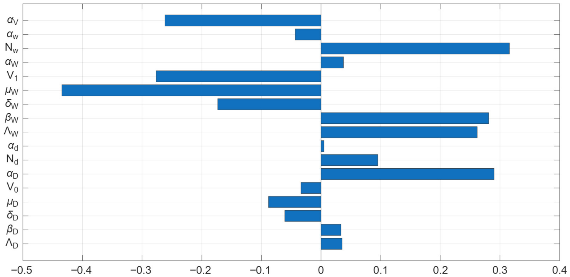
In this section, a global sensitivity analysis was performed to evaluate how variations in model parameters affect the basic reproduction number, $R_0$, of the system (1). Parameter values are listed in Table 2, and the analysis used Latin Hypercube Sampling (LHS) combined with partial rank correlation coefficients (PRCCs) over 1000 simulations.

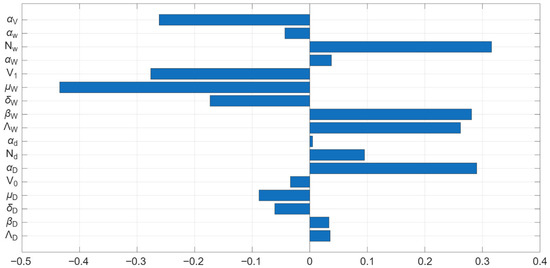
Figure 2 shows a tornado plot of the PRCCs, indicating both the strength and direction of each parameter’s influence on $R_0$: positive values increase viral transmission potential, while negative values reduce $R_0$ and suppress transmission. The results identify the most influential parameters driving viral spread in the model. The disease is primarily driven by parameters that strongly affect viral transmission. Increases in wild host population ($N_W$), transmission rates (${\alpha }_D$, ${\beta }_W$), and host recruitment (${\Lambda }_W$) enhance $R_0$ and promote spread. Conversely, higher wild host mortality (${\mu }_W$), vaccination ($V_1$), virus clearance (${\alpha }_V$), and disease-induced mortality (${\delta }_W$) reduce $R_0$ and limit transmission. These findings identify critical targets for interventions aimed at controlling the outbreak. Overall, the identified parameters play a significant role in the transmission dynamics of FMD and are therefore essential for effective infection management throughout the pathogen’s transmission cycle. Consequently, these parameters should be carefully considered and appropriately managed during outbreak response at the hosts level.

Figure 2. Tornado plot of partial rank correlation coefficients (PRCCs) of all the model parameters that influence the viral transmission metric $R_0$.

5. Numerical Analysis

To complement the theoretical analysis and gain deeper insight into the epidemiological implications of the model, numerical simulations of system (1) were performed using MATLAB R2023b. These simulations examined how variations in key transmission and progression parameters, including ${\beta }_D$, ${\beta }_W$, ${\alpha }_D$, ${\alpha }_W$, $N_D$, $N_W$, and ${\alpha }_V$, affect the dynamics of domestic and wild ruminant populations, as well as the accumulation and decay of community viral load ($V_E$) that mediates indirect transmission. The analysis served not only to validate the mathematical results derived in Section 3 but also to provide a deeper understanding of the mechanisms sustaining FMD within a coupled livestock–wildlife–environment system. Numerical simulations were implemented using the Nonstandard Finite Difference (NSFD) method, chosen for its ability to preserve essential model properties such as positivity and stability, which are critical in studying infectious disease dynamics. The model incorporates compartments for susceptible, exposed, and infected individuals in both domestic and wild populations, along with the environmental viral load representing the overall community viral burden. The initial conditions for the simulations were set as $S_W=80$, $E_W=10$, $I_W=10$, $S_D=70$, $E_D=15$, $I_D=15$, and $V_E=2000$, providing a baseline for exploring the temporal evolution of the system and assessing the effects of key parameters on FMD transmission and persistence.

5.1. Numerical Methods

This section presents the construction of the Nonstandard Finite Difference (NSFD) scheme for Equations (1)–(7). This scheme is primarily designed to guarantee unconditional stability and preserve positivity in the variables representing the subpopulations $S_W\left(t\right)$, $S_D\left(t\right)$, $E_W\left(t\right)$, $E_D\left(t\right)$, $I_W\left(t\right)$, $I_D\left(t\right)$, and $V_E\left(t\right)$. The NSFD scheme, introduced by Ronald E. Mickens, is a numerical technique used to discretize differential equations while preserving key qualitative properties of the original continuous system, properties that are often lost in standard numerical methods. We use the symbols $S_W\left(t\right)$, $S_D\left(t\right)$, $E_W\left(t\right)$, $E_D\left(t\right)$, $I_W\left(t\right)$, $I_D\left(t\right)$, and $V_E\left(t\right)$ to represent the estimated values of $S_W\left(kh\right)$, $S_D\left(kh\right)$, $E_W\left(kh\right)$, $E_D\left(kh\right)$, $I_W\left(kh\right)$, $I_D\left(kh\right)$, and $V_E\left(kh\right)$, respectively, for values of $k=0,1,2,\dots$, and with a constant h representing the time step of the scheme where $h>0$. For the sequences $S_W\left(t\right)$, $S_D\left(t\right)$, $E_W\left(t\right)$, $E_D\left(t\right)$, $I_W\left(t\right)$, $I_D\left(t\right)$, and $V_E\left(t\right)$ to be consistent with the model’s biological nature, the equations should be non-negative [36]. Generally, a standard finite difference scheme approximates a derivative as:

$${\displaystyle \frac{dy}{dt}}\approx {\displaystyle \frac{y_{k+1}-y_k}{h}}.$$

But in an NSFD scheme, the denominator is replaced with a nonlinear function ${\varphi }_h$ that better captures the system’s dynamics:

$${\displaystyle \frac{dy}{dt}}\approx {\displaystyle \frac{y_{k+1}-y_k}{{\varphi }_h}},$$

where ${\varphi }_h\to h.$

The two fundamental principles upon which nonstandard schemes are based can be briefly stated as follows:

$$\begin{array}{c}\hfill \left\{\begin{array}{ccc}& & 1.{\displaystyle \frac{S_D^{(k+1)}-S_D^k}{{\psi }_1}}={\Lambda }_D-{\displaystyle \frac{{\beta }_D{V}_E^k{S}_D^{k+1}}{V_0+V_E^k}}-{\mu }_D{S}_D^{(k+1)},\hfill \\ & & \\ & & 2.{\displaystyle \frac{E_D^{(k+1)}-E_D^{\left(k\right)}}{{\psi }_2}}={\displaystyle \frac{{\beta }_D{V}_E^k{S}_D^{k+1}}{V_0+V_E^k}}-({\mu }_D+{\alpha }_D)E_D^{k+1},\hfill \\ & & \\ & & 3.{\displaystyle \frac{I_D^{k+1}-I_D^k}{{\psi }_3}}={\alpha }_D{E}_D^{k+1}-({\mu }_D+{\delta }_D)I_D^{k+1},\hfill \\ & & \\ & & 4.{\displaystyle \frac{V_E^{k+1}-V_E^k}{{\psi }_4}}=N_D{\alpha }_D{I}_D^{k+1}+N_W{\alpha }_W{I}_W^{k+1}-{\alpha }_V{V}_E^{k+1},\hfill \\ & & \\ & & 5.{\displaystyle \frac{S_W^{k+1}-S_W^k}{{\psi }_5}}={\Lambda }_W-{\displaystyle \frac{{\beta }_W{V}_E^k{S}_W^{k+1}}{V_0+V_E^k}}-{\mu }_W{S}_W^{k+1},\hfill \\ & & \\ & & 6.{\displaystyle \frac{E_W^{k+1}-E_W^k}{{\psi }_6}}={\displaystyle \frac{{\beta }_D{V}_E^k{E}_W^{k+1}}{V_0+V_E^k}}-({\mu }_W+{\alpha }_W)E_W^{k+1},\hfill \\ & & \\ & & 7.{\displaystyle \frac{I_W^{k+1}-I_W^k}{{\psi }_7}}={\alpha }_W{E}_W^{k+1}-({\mu }_W+{\delta }_W)I_W^{k+1}.\hfill \end{array}\right.\end{array}$$

(72)

Below are the denominator functions considered in this study:

$$\begin{array}{c}\hfill \left\{\begin{array}{ccc}& {\psi }_1& ={\displaystyle \frac{e^{{\mu }_{D}h}-1}{{\mu }_D}},\hfill \\ & {\psi }_2& ={\displaystyle \frac{e^{({\mu }_D+{\alpha }_D)h}-1}{{\mu }_D+{\alpha }_D}},\hfill \\ & {\psi }_3& ={\displaystyle \frac{e^{({\mu }_D+{\delta }_D)h}-1}{{\mu }_D+{\delta }_D}},\hfill \\ & {\psi }_4& ={\displaystyle \frac{e^{{\alpha }_{V}h}-1}{{\alpha }_V}},\hfill \\ & {\psi }_5& ={\displaystyle \frac{e^{{\mu }_{W}h}-1}{{\mu }_W}},\hfill \\ & {\psi }_6& ={\displaystyle \frac{e^{({\mu }_W+{\alpha }_W)h}-1}{{\mu }_W+{\alpha }_W}},\hfill \\ & {\psi }_7& ={\displaystyle \frac{e^{({\mu }_W+{\delta }_W)h}-1}{{\mu }_W+{\delta }_W}}.\hfill \end{array}\right.\end{array}$$

Rearranging (72), we obtain the following explicit scheme

$$\begin{array}{c}\hfill \left\{\begin{array}{ccc}& & 1.S_D^{(k+1)}={\displaystyle \frac{S_D^k+{\psi }_1{\Lambda }_D}{{\displaystyle 1+{\psi }_1{\mu }_D+{\psi }_1\frac{{\beta }_D{V}_E^k}{V_0+V_E^k}}}},\hfill \\ & & \\ & & 2.E_D^{(k+1)}={\displaystyle \frac{{\displaystyle E_D^{\left(k\right)}+{\psi }_2\frac{{\beta }_D{V}_E^k{S}_D^{k+1}}{V_0+V_E^n}}}{1+{\psi }_2({\mu }_D+{\alpha }_D)}},\hfill \\ & & \\ & & {\displaystyle 3.I_D^{(k+1)}=\frac{I_D^{\left(k\right)}+{\psi }_3{\alpha }_D{E}_D^{k+1}}{1+{\psi }_3({\mu }_D+{\delta }_D)},}\hfill \\ & & \\ & & 4.V_E^{(k+1)}={\displaystyle \frac{V_E^{\left(k\right)}+{\psi }_4\left(N_D{\alpha }_D{I}_D^{k+1}+N_W{\alpha }_W{I}_W^{k+1}\right)}{1+{\psi }_4{\alpha }_V}},\hfill \\ & & \\ & & 5.S_W^{(k+1)}={\displaystyle \frac{S_W^{\left(k\right)}+{\psi }_5{\Lambda }_W}{{\displaystyle 1+{\psi }_5{\mu }_W+{\psi }_5\frac{{\beta }_W{V}_E^k}{V_0+V_E^k}}}},\hfill \\ & & \\ & & 6.E_W^{(k+1)}={\displaystyle \frac{E_W^{\left(k\right)}}{1-{\psi }_6{\displaystyle \frac{{\beta }_D{V}_E^k}{V_0+V_E^k}}+{\psi }_6({\mu }_W+{\alpha }_W)}},\hfill \\ & & \\ & & 7.I_W^{k+1}={\displaystyle \frac{I_W^k+{\psi }_7{\alpha }_W{E}_W^{k+1}}{1+{\psi }_7({\mu }_W+{\delta }_W)}}.\hfill \end{array}\right.\end{array}$$

(73)

Equation (73) must be evaluated sequentially, as the computation of $S_D^{(k+1)}$ provides the input for determining $E_D^{(k+1)}$. The value of $I_D^{(k+1)}$ is subsequently required for the evaluation of $V_E^{(k+1)}$, which in turn is used to compute $S_W^{(k+1)}$. This iterative procedure is carried out successively until the prescribed terminal time is attained.

5.2. Numerical Simulations

5.2.1. Intrinsic Population Dynamics for FMD Dynamics

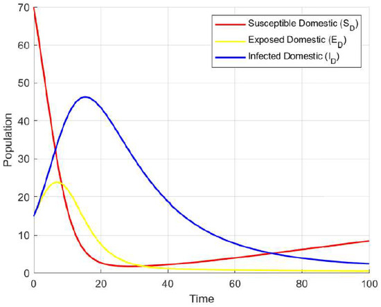
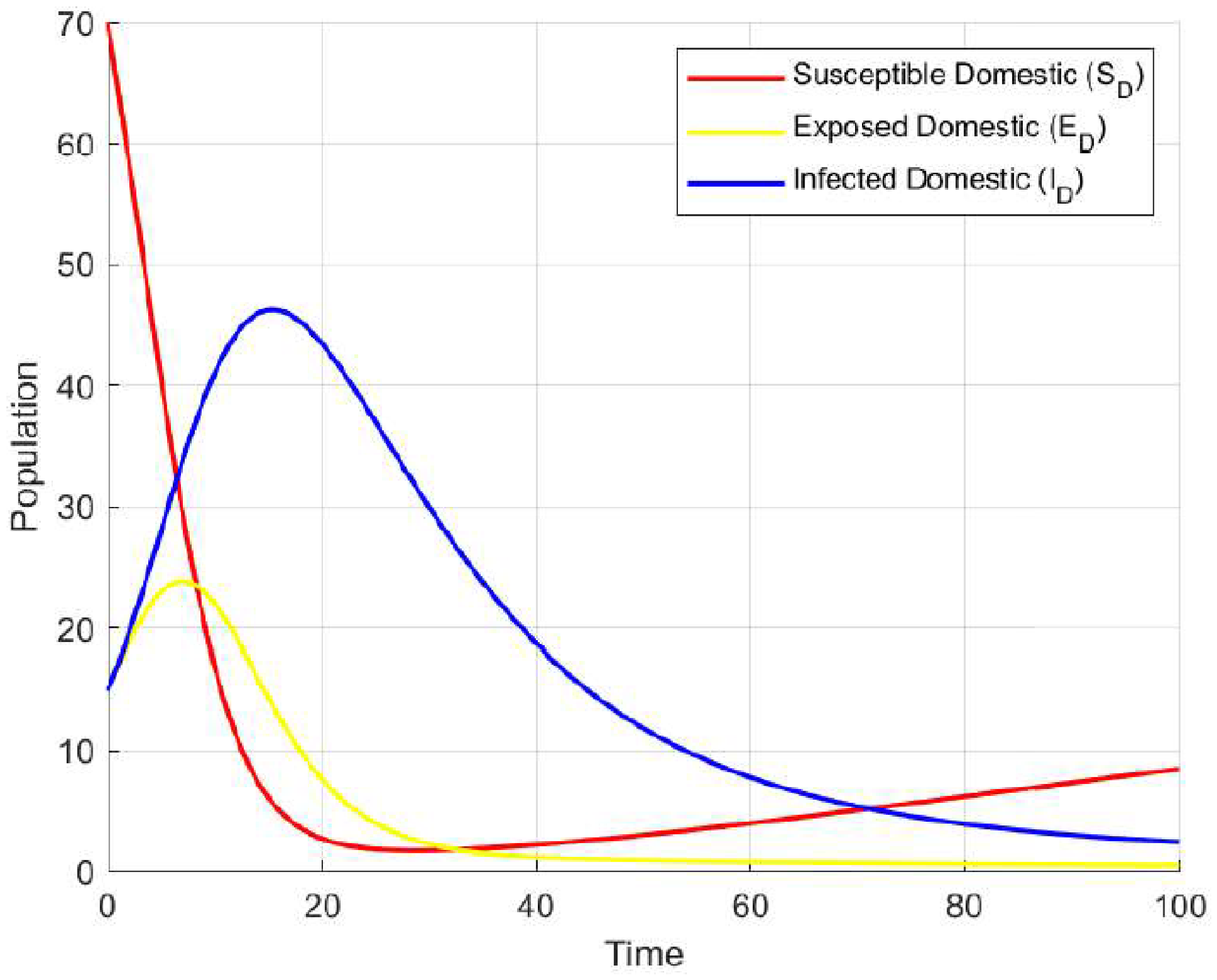
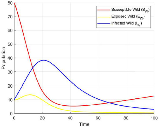
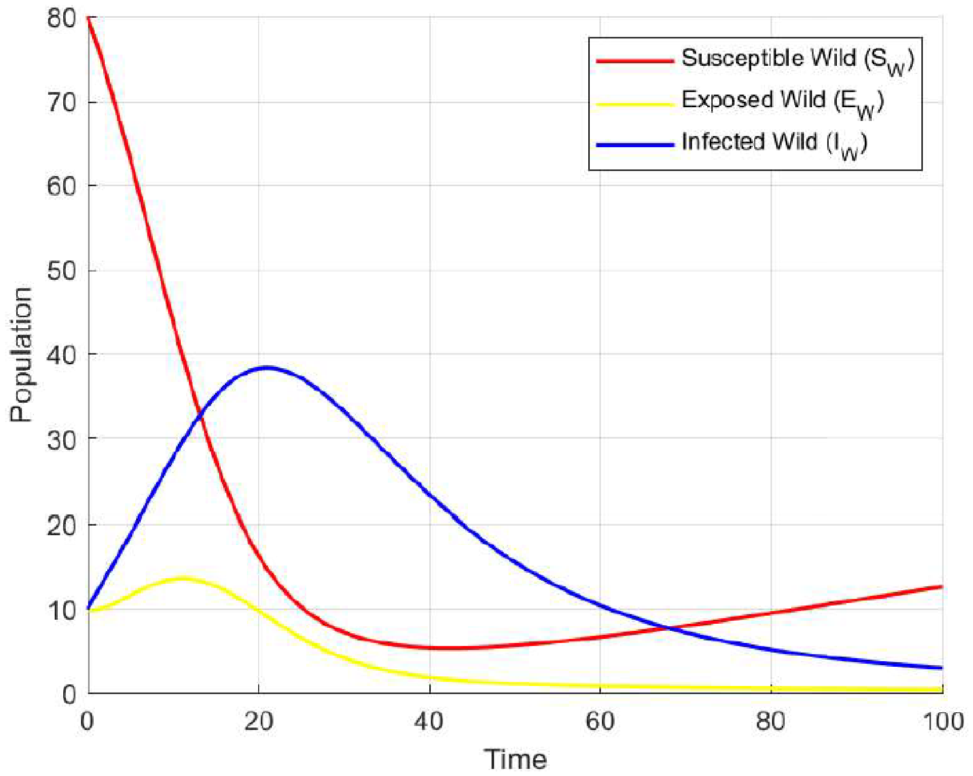
In this subsection, we present plots showing numerical solutions for the model system (1), illustrating the intrinsic population dynamics of both the domestic and wild animals under the influence of FMD. Figure 3 shows the evolution in time of the population dynamics of domestic animals in the presence of the FMD and Figure 4 illustrates the evolution in time of the population dynamics of different stages of FMD transmission between domestic and wild animals.

Figure 3. Simulation of model system (1) showing the dynamics of a domestic population with initial conditions: $S_D\left(0\right)$ = 70, $I_D\left(0\right)$ = 15, $E_D\left(0\right)$ = 15.

Figure 4. Simulation of model system (1) showing the dynamics of a wild population with initial conditions: $S_W\left(0\right)$ = 80, $I_W\left(0\right)$ = 10, $E_W\left(0\right)$ = 10.

The simulation results of the FMD model system (1) presented in Figure 3 show the temporal dynamics of domestic ruminants under FMD. The susceptible population ($S_D$) declines as individuals become exposed and subsequently infected. The exposed class ($E_D$) rises briefly before stabilizing as animals progress to the infectious state. The infected population ($I_D$) peaks early in the outbreak, reflecting active transmission, then declines as susceptibles are depleted. These trends highlight the role of viral shedding in maintaining the community viral load and driving disease progression within the domestic population.

Figure 4 illustrates FMD transmission across domestic and wild animals. The rise in exposed and infected individuals shows active transmission between populations, mediated by direct contact and environmental viral contamination. Infection levels eventually decline as susceptible animals decrease, demonstrating the interplay between population depletion and viral spread. The results emphasize how the community viral load facilitates cross-species transmission and sustains the outbreak.

5.2.2. Influence of FMD Intervention on the Disease Dynamics

In this section, we explore the influence of seven selected key parameters of the model system (1), ${\beta }_D$, ${\beta }_W$, ${\alpha }_D$, ${\alpha }_W$, $N_D$, $N_W$, and ${\alpha }_D$, on the system’s six variables ($S_D$, $E_D$, $I_D$, $S_W$, $E_W$, $I_W$). Numerical simulations were performed to verify the analytical results obtained in Section 3 and to examine how variations in key epidemiological parameters influence the transmission dynamics and persistence of the virus. By varying these parameters, we gain a better understanding of their roles in driving disease spread and identify those that have the greatest impact on FMD dynamics, thereby providing useful insights for designing interventions aimed at controlling and reducing FMD transmission within the community.

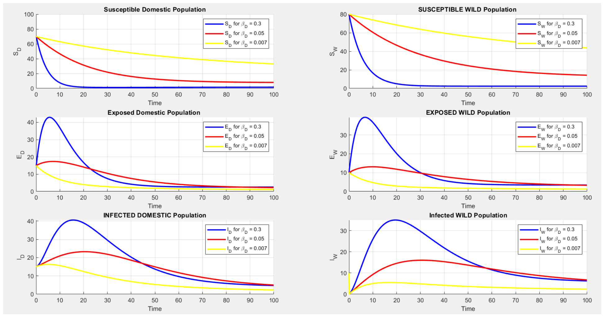
Figure 5 illustrates the effect of varying the infection rate associated with the domestic animal population (${\beta }_D$) on both domestic ($S_D$, $E_D$, $I_D$) and wild ($S_W$, $E_W$, $I_W$) ruminant population dynamics. As ${\beta }_D$ increases, the number of susceptible individuals in both populations declines rapidly, reflecting higher exposure to FMD. This accelerated transition from susceptible to exposed and infected classes also increases the community viral load, which drives transmission within and between populations. The results highlight the critical impact of high transmission rates on overall population health and emphasize the importance of interventions aimed at reducing viral spread to protect both livestock and wildlife.

Figure 5. Graphs of numerical solutions of model system (1) showing the evolution in time of domestic and wild animal populations for different values of the transmission rate between wild population and the environment ${\beta }_W$: ${\beta }_D$ = 0.2, ${\beta }_D$ = 0.03, ${\beta }_D$ = 0.007.

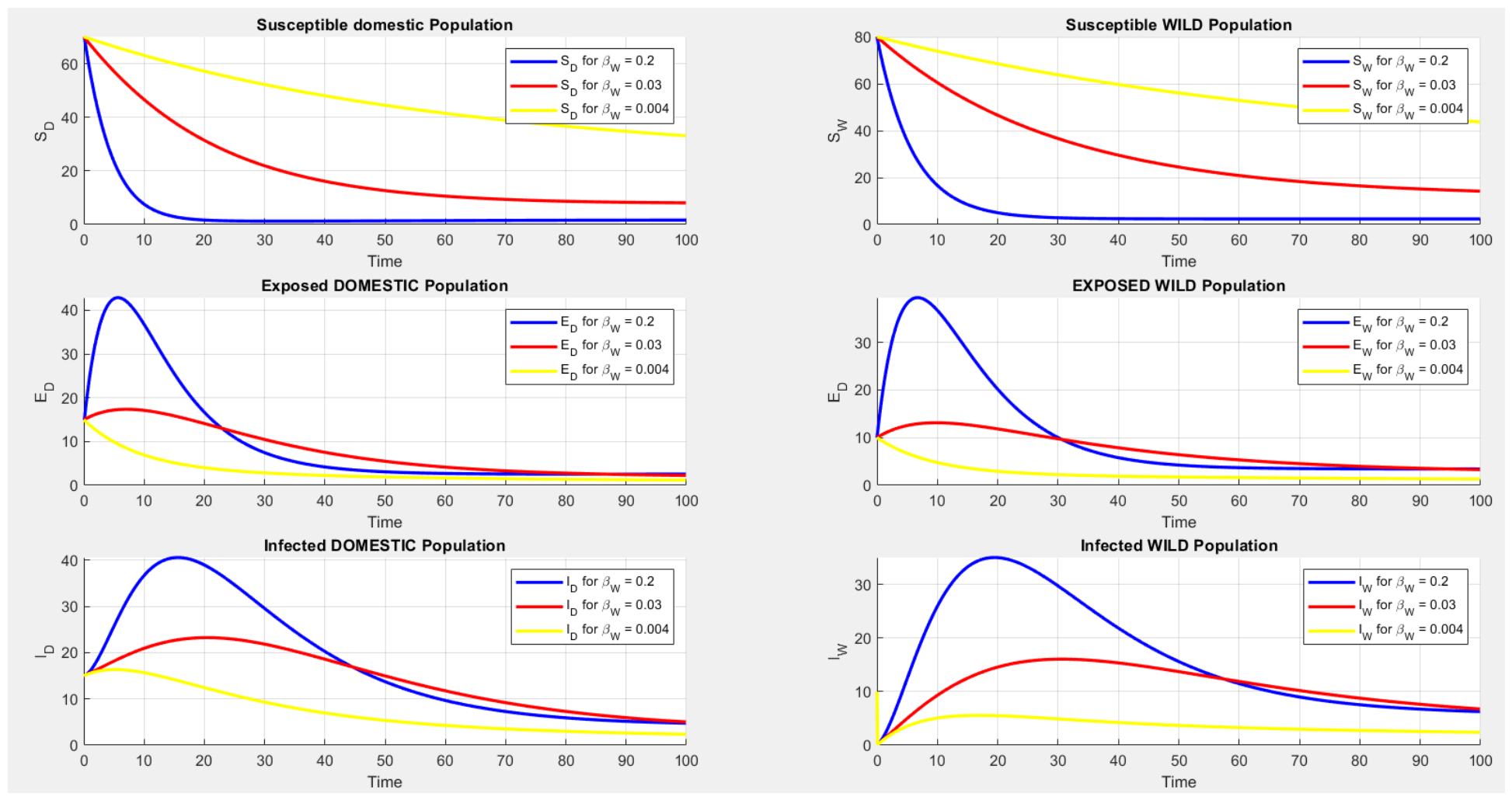
Figure 6 illustrates the effect of varying the infection rate associated with the wild animal population (${\beta }_W$) on the dynamics of the wild ruminant population variables ($S_W$, $E_W$, $I_W$) and the domestic ruminant population variables ($S_D$, $E_D$, $I_D$). The simulations are presented for different values of ${\beta }_W$: ${\beta }_W$ = 0.2, ${\beta }_W$ = 0.03, ${\beta }_W$ = 0.004. As ${\beta }_W$ increases, the number of susceptible individuals in both populations declines rapidly, indicating increased exposure to FMD. Higher transmission from the wild population leads to more infected individuals.

Figure 6. Graphs of numerical solutions of model system (1) showing the evolution in time of domestic and wild animal populations for different values of the transmission rate between wild population and the environment ${\beta }_W$: ${\beta }_W$ = 0.2, ${\beta }_W$ = 0.03, ${\beta }_W$ = 0.004.

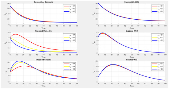
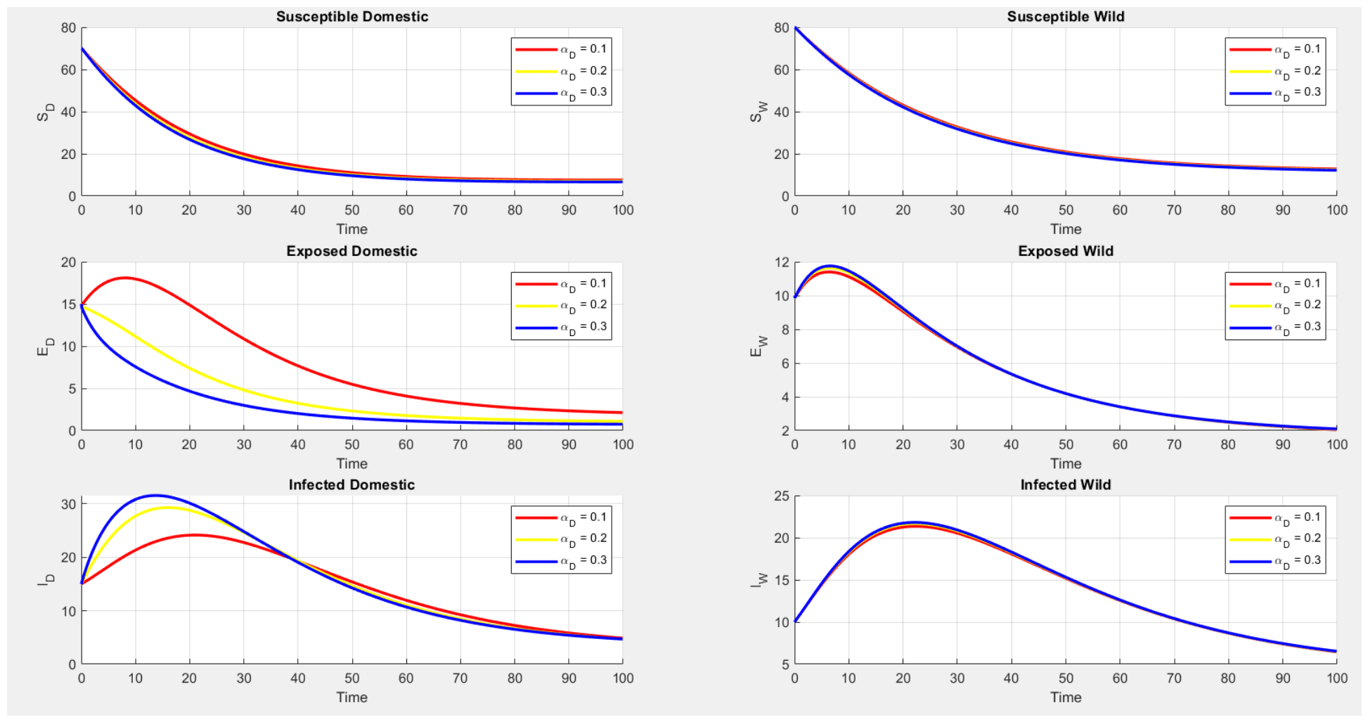
Figure 7 illustrates the effect of varying the progression rate from the exposed to the infectious state for the domestic animal population (${\alpha }_D$) on both the domestic ruminant variables ($S_D$, $E_D$, $I_D$) and the wild ruminant variables ($S_W$, $E_W$, $I_W$). The simulations are presented for different values of ${\alpha }_D$: 0.1, 0.2, and 0.3. As ${\alpha }_D$ increases, exposed domestic animals progress more rapidly to the infectious class, leading to noticeable changes in the domestic population dynamics. This increase in infectious individuals enhances viral shedding, thereby contributing to the community viral load and promoting transmission within the domestic population. In contrast, the effect on the wild population remains relatively small. These results suggest that interventions aimed at slowing the progression from exposure to infection in domestic animals could reduce the burden of FMD within domestic herds while having only limited effects on the wild population.

Figure 7. Graphs of numerical solutions of model system (1) showing the evolution in time of domestic and wild population for different values of the rate at which exposed domestic animals become infected ${\alpha }_D$: ${\alpha }_D$ = 0.1, ${\alpha }_D$ = 0.2, ${\alpha }_D$ = 0.3.

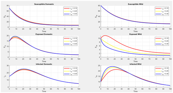
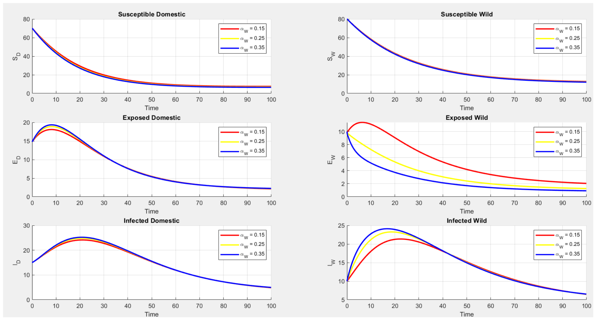
Figure 8 illustrates the effect of varying the progression rate from the exposed to the infectious state for the wild animal population (${\alpha }_W$) on both the wild ruminant variables ($S_W$, $E_W$, $I_W$) and the domestic ruminant variables ($S_D$, $E_D$, $I_D$). The simulations are presented for different values of ${\alpha }_W$: 0.15, 0.25, and 0.35. As ${\alpha }_W$ increases, exposed wild animals progress more rapidly to the infectious class, leading to noticeable changes in the dynamics of the wild population. This increase in infectious wild animals contributes to the community viral load, which can facilitate environmental transmission. However, the impact on the domestic population remains relatively small. These results suggest that reducing the progression of infection among wild animals could help lower the burden of FMD in wildlife populations, with only limited effects on domestic animals.

Figure 8. Graphs of numerical solutions of model system (1) showing the evolution in time of domestic and wild population for different values of the rate at which exposed domestic animals become infected ${\alpha }_W$: ${\alpha }_W$ = 0.15, ${\alpha }_W$ = 0.25, ${\alpha }_W$ = 0.35.

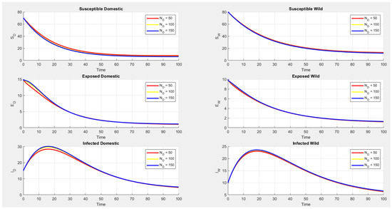
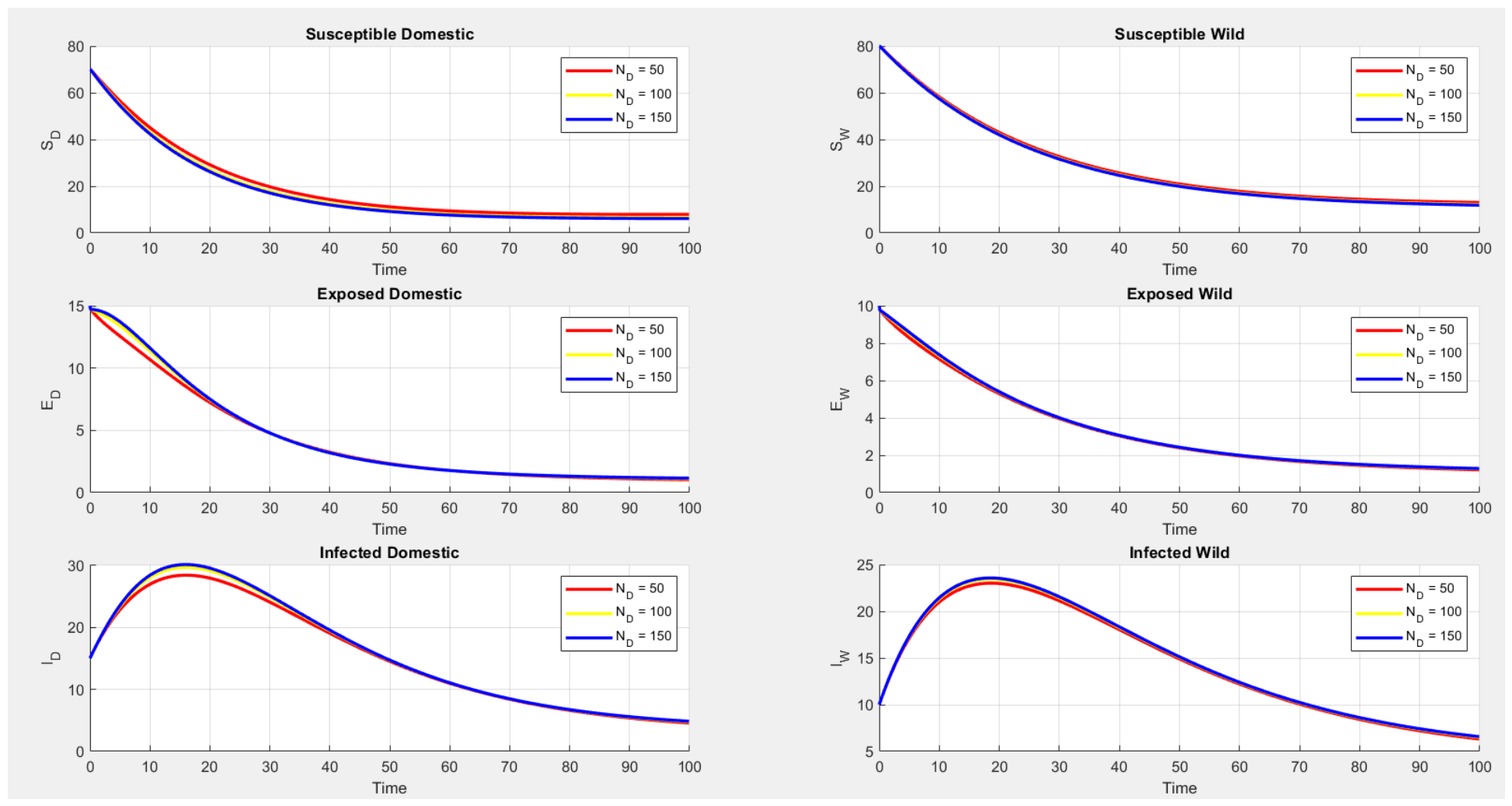
Figure 9 illustrates the effect of varying the average FMD community viral load contributed by domestic animals ($N_D$) on the temporal dynamics of both domestic and wild ruminant populations. The figure presents the evolution of the domestic variables ($S_D$, $E_D$, $I_D$) and the wild variables ($S_W$, $E_W$, $I_W$) for different values of $N_D$: 50, 100, and 150. As $N_D$ increases, only a slight change is observed in the dynamics of both populations. This indicates that increases in the community viral load originating from domestic animals produce relatively small changes in disease transmission within and between the two populations. Consequently, interventions aimed solely at reducing the domestic contribution to the community viral load may have a limited impact on controlling the spread of FMD.

Figure 9. The effect of varying the average number of FMD community viral loads due to domestic animals on evolution in time of domestic and wild population for different values of $N_D$: $N_D=50$, $N_D$: $N_D=100$ and $N_D$: $N_D=150$.

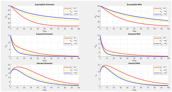
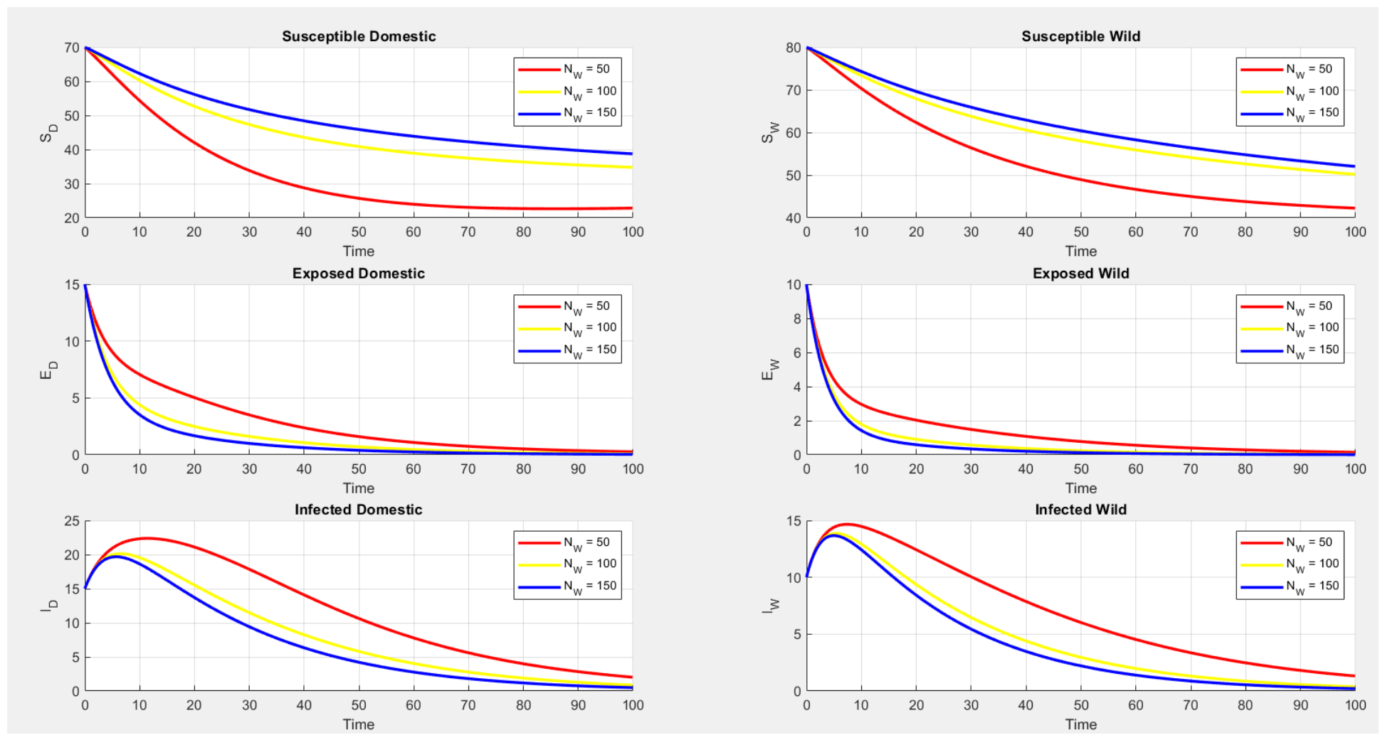
Figure 10 illustrates the effect of varying the average FMD community viral load contributed by wild animals ($N_W$) on the temporal dynamics of both wild and domestic ruminant populations. The figure shows the evolution of the wild variables ($S_W$, $E_W$, $I_W$) and the domestic variables ($S_D$, $E_D$, $I_D$) for different values of $N_W$: 50, 100, and 150. As $N_W$ increases, noticeable changes occur in the dynamics of both populations, with higher infection levels observed among wild and domestic animals. This indicates that increases in the community viral load originating from wild animals can enhance transmission within and between the two populations. Consequently, interventions aimed at reducing the viral load contributed by wild animals may play an important role in mitigating the spread of FMD.

Figure 10. The effect of varying the average number of FMD community viral loads due to domestic animals on evolution in time of domestic and wild population for different values of $N_W$: $N_W=50$, $N_W=100$ and $N_W=150$.

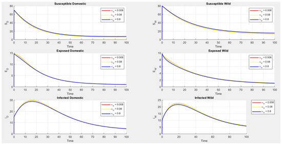
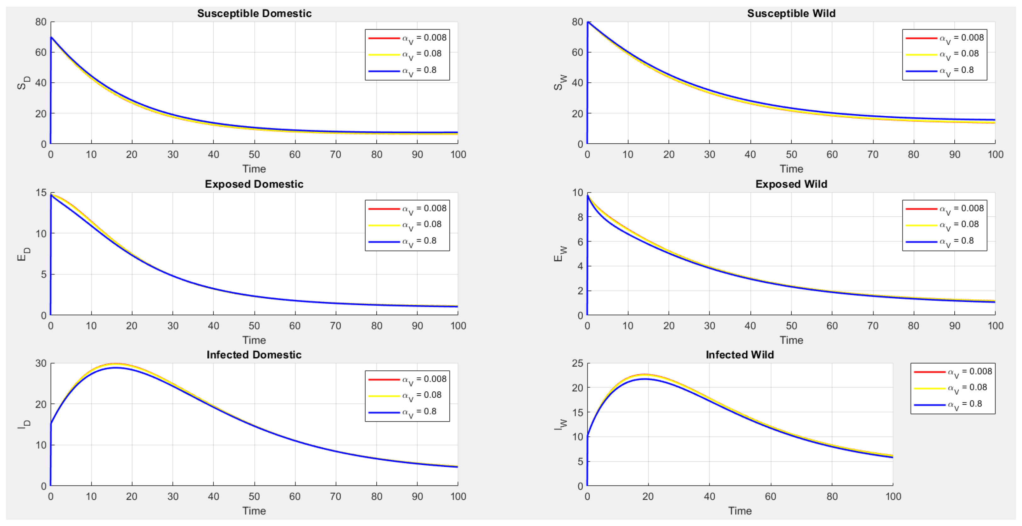
Figure 11 illustrates the numerical solutions of the model system (1), showing the temporal dynamics of both domestic and wild ruminant populations. The figure presents the evolution of the domestic variables ($S_D$, $E_D$, $I_D$) and the wild variables ($S_W$, $E_W$, $I_W$) for different values of the viral decay rate ${\alpha }_V$: 0.008, 0.08, and 0.8. The results indicate that variations in the decay rate of the FMD community viral load produce only modest changes in the population dynamics of both domestic and wild animals. This suggests that increasing the rate at which the virus decays in the environment may reduce viral persistence, but its overall effect on the population dynamics and transmission between the two populations remains limited.

Figure 11. Graphs of numerical solutions of model system (1) showing the evolution in time of domestic and wild populations for different values of viral decay rate in the environment ${\alpha }_V$: ${\alpha }_V$ = 0.008, ${\alpha }_V$ = 0.08, ${\alpha }_V$ = 0.8.

6. Discussion and Conclusions

The model was formulated using a Susceptible–Exposed–Infected (SEI) framework extended with a free-living virus compartment to capture environmental persistence and indirect transmission. In line with the aim of this study to investigate the extent to which community viral load sustains FMD persistence and identify key drivers of transmission, this formulation provides a novel perspective by explicitly incorporating community viral load and environmental viral decay within a multi-host livestock wildlife framework. This allows the role of environmental contamination in sustaining FMD outbreaks to be examined more explicitly.

The basic reproduction number ($R_0$) was derived to assess equilibrium stability, with $R_0<1$ indicating disease fade-out and $R_0>1$ implying sustained transmission. Sensitivity analysis using partial rank correlation coefficients (PRCCs) identified the parameters most influential on $R_0$. Increases in wild host population size ($N_W$), transmission rates (${\beta }_W$, ${\alpha }_D$), and host recruitment (${\Lambda }_W$) enhanced $R_0$ and promoted viral spread, whereas higher wild host mortality (${\mu }_W$), virus clearance (${\alpha }_V$), FMD viral load threshold for wild infection ($V_1$), and disease-induced mortality (${\delta }_W$) reduced $R_0$ and limited transmission. Parameters associated with community viral load ($N_D$, $N_W$) and environmental viral decay (${\alpha }_V$) were particularly critical, confirming that the accumulation and persistence of viral load are central to sustaining indirect transmission, with wildlife contributions exerting a stronger effect than domestic populations.

Numerical simulations using the NSFD method confirmed these findings: higher transmission rates accelerated declines in susceptible populations and increased the exposed and infected classes, while progression rates primarily influenced their respective populations. These results support the study’s aim by demonstrating how community viral load mediates interactions between domestic and wild populations and sustains disease transmission through environmental persistence. Integrating environmental viral load dynamics with both domestic and wild host populations provides new insight into how indirect transmission pathways contribute to FMD persistence.

Combining sensitivity analysis, $R_0$, and numerical simulations demonstrates that incorporating both direct host-to-host transmission and community viral load provides a robust framework for understanding FMD persistence and guiding targeted interventions. These findings offer practical guidance for reducing transmission intensity and environmental viral load, even in resource-limited settings with limited recovery data.

Our results align with previous studies such as in [37,38,39,40], confirming that interactions among wildlife, livestock, and the environment drive FMD transmission. They emphasize the importance of targeting interventions to reduce transmission, manage viral load, and control wildlife–livestock interfaces. Unlike many previous models that focus primarily on direct transmission, this study fulfills its aim by explicitly quantifying the contribution of community viral load and viral threshold dynamics in a coupled livestock–wildlife system, thereby extending existing modeling approaches. Although recovery dynamics were not included due to data limitations, the model provides a theoretical basis for informing control strategies and maintaining healthy domestic and wild animal populations.

Future research should integrate recovery dynamics, environmental factors, and economic considerations to develop more comprehensive and effective strategies for controlling FMD. Incorporating recovery dynamics will enhance understanding of how animals regain health, the duration of recovery, and the time required for their return to production. Accounting for environmental influences, such as climate variability, habitat conditions, and seasonal patterns, will provide a more complete perspective on the factors driving FMD outbreaks. Moreover, assessing the economic impacts, including the costs of vaccination programs, losses in livestock productivity, and broader effects on markets and supply chains, will enable more balanced and sustainable planning. By combining these aspects, future studies can provide policymakers and stakeholders with the insights needed to design evidence-based interventions that improve animal health, strengthen biosecurity, and support agricultural sustainability.

References

- Woolhouse, M.; Donaldson, A. Managing foot-and-mouth. Nature 2001, 410, 515–516. [Google Scholar] [CrossRef] [Scilit]
- Fair, K.R.; Bauch, C.T.; Anand, M. Dynamics of the global wheat trade network and resilience to shocks. Sci. Rep. 2017, 7, 7177. [Google Scholar] [CrossRef] [Scilit] [PubMed]
- Stockdale, J.E.; Liu, P.; Colijn, C. The potential of genomics for infectious disease forecasting. Nat. Microbiol. 2022, 7, 1736–1743. [Google Scholar] [CrossRef] [Scilit]
- Sobrino, F.; Sáiz, M.; Jiménez-Clavero, M.A.; Núñez, J.I.; Rosas, M.F.; Baranowski, E.; Ley, V. Foot-and-mouth disease virus: A long known virus, but a current threat. Vet. Res. 2001, 32, 1–30. [Google Scholar] [CrossRef] [Scilit] [PubMed]
- Mwiine, F.N.; Ayebazibwe, C.; Olaho-Mukani, W.; Alexandersen, S. Persistence of foot-and-mouth disease virus in African buffalo (Syncerus caffer) in Uganda. PLoS ONE 2019, 14, e0209658. [Google Scholar]
- Henning, A.; Odendaal, L.; Loots, A.; Quan, M. Demonstrating persistence of foot-and-mouth disease virus in African buffalo (Syncerus caffer) using BaseScope™ in situ hybridisation. Vet. Res. Commun. 2025, 49, 324. [Google Scholar] [CrossRef] [Scilit] [PubMed]
- Dixon, S.M. Collaborative Response and Recovery from a Foot-and-Mouth Disease Animal Health Emergency: Supporting Decision Making in a Complex Environment with Multiple Stakeholders; Naval Postgraduate School: Monterey, CA, USA, 2013. [Google Scholar]
- Alexandersen, S.; Zhang, Z.; Donaldson, A.I.; Garland, A.J.M. The pathogenesis and diagnosis of foot-and-mouth disease. J. Comp. Pathol. 2003, 129, 1–36. [Google Scholar] [CrossRef] [Scilit]
- Grubman, M.J.; Baxt, B. Foot-and-mouth disease. Clin. Microbiol. Rev. 2004, 17, 465–493. [Google Scholar] [CrossRef] [Scilit]
- Knight-Jones, T.J.D.; Rushton, J. The economic impacts of foot and mouth disease—What are they, how big are they and where do they occur? Prev. Vet. Med. 2013, 112, 161–173. [Google Scholar] [CrossRef] [Scilit]
- Paton, D.J.; Sumption, K.J.; Charleston, B. Foot-and-mouth disease virus: A long known but still dangerous foe. Infect. Genet. Evol. 2009, 9, 229–240. [Google Scholar]
- Domingo, E.; Baranowski, E.; Escarmís, C.; Sobrino, F. Foot-and-mouth disease virus. Comp. Immunol. Microbiol. Infect. Dis. 2003, 26, 297–308. [Google Scholar]
- World Organization for Animal Health (OIE). Foot-and-Mouth Disease; OIE: Paris, France, 2016; Available online: https://www.woah.org/en/disease/foot-and-mouth-disease/ (accessed on 29 January 2026).
- Keeling, M.J.; Woolhouse, M.E.J.; Shaw, D.J.; Matthews, L.; Chase-Topping, M.; Haydon, D.T.; Cornell, S.J.; Kappey, J.; Wilesmith, J.; Grenfell, B.T. Dynamics of the 2001 UK foot and mouth epidemic: Stochastic dispersal in a heterogeneous landscape. Science 2001, 294, 813–817. [Google Scholar] [CrossRef] [Scilit]
- Tildesley, M.J.; Savill, N.J.; Shaw, D.J.; Deardon, R.; Brooks, S.P.; Woolhouse, M.E.J.; Grenfell, B.T.; Keeling, M.J. Optimal reactive vaccination strategies for an outbreak of foot-and-mouth disease in Great Britain. Nature 2006, 440, 83–86. [Google Scholar] [CrossRef] [Scilit]
- Cardenas, N.C.; Lopes, F.P.N.; Machado, A.; Maran, V.; Trois, C.; Machado, F.A.; Machado, G. Modeling foot-and-mouth disease dissemination in Rio Grande do Sul, Brazil and evaluating the effectiveness of control measures. Front. Vet. Sci. 2024, 11, 1468864. [Google Scholar] [CrossRef] [Scilit] [PubMed]
- Chase-Topping, M.E.; Handel, I.; Bankowski, B.M.; Juleff, N.D.; Gibson, D.; Cox, S.J.; Windsor, M.A.; Reid, E.; Doel, C.; Howey, R.; et al. Understanding foot-and-mouth disease virus transmission biology: Identification of the indicators of infectiousness. Vet. Res. 2013, 44, 46. [Google Scholar] [PubMed]
- Guerra, F.M.; Bolotin, S.; Lim, G.; Heffernan, J.; Deeks, S.L.; Li, Y.; Crowcroft, N.S. The basic reproduction number (R0) of measles: A systematic review. Lancet Infect. Dis. 2017, 17, e420–e428. [Google Scholar] [CrossRef] [Scilit]
- Aslam, M.; Alkheraije, K.A. The prevalence of foot-and-mouth disease in Asia. Front. Vet. Sci. 2023, 10, 1201578. [Google Scholar]
- Bernstein, A.S.; Ando, A.W.; Loch-Temzelides, T.; Vale, M.M.; Li, B.V.; Li, H.; Busch, J.; Chapman, C.A.; Kinnaird, M.; Nowak, K.; et al. The costs and benefits of primary prevention of zoonotic pandemics. Sci. Adv. 2022, 8, eabl4183. [Google Scholar] [CrossRef] [Scilit]
- La, A.; Zhang, Q.; Cicek, N.; Coombs, K.M. Current understanding of the airborne transmission of important viral animal pathogens in spreading disease. Biosyst. Eng. 2022, 224, 92–117. [Google Scholar] [CrossRef] [Scilit]
- Belsham, G.J. Towards improvements in foot-and-mouth disease vaccine performance. Acta Vet. Scand. 2020, 62, 20. [Google Scholar] [CrossRef] [Scilit]
- Kao, R.R.; Danon, L.; Green, D.M.; Kiss, I.Z. Demographic structure and pathogen dynamics on the network of livestock movements in Great Britain. Proc. R. Soc. B 2006, 273, 1999–2007. [Google Scholar] [CrossRef] [Scilit]
- Ringa, N.; Bauch, C.T. Impacts of constrained culling and vaccination on control of foot and mouth disease in near-endemic settings: A pair approximation model. Epidemics 2014, 9, 18–30. [Google Scholar] [CrossRef] [Scilit] [PubMed]
- Souley Kouato, B.; De Clercq, K.; Abatih, E.; Dal Pozzo, F.; King, D.P.; Thys, E.; Marichatou, H.; Saegerman, C. Review of epidemiological risk models for foot-and-mouth disease: Implications for prevention strategies with a focus on Africa. PLoS ONE 2018, 13, e0208296. [Google Scholar]
- Humphreys, J.M.; Stenfeldt, C.; King, D.P.; Knight-Jones, T.; Perez, A.M.; VanderWaal, K.; Sanderson, M.W.; Di Nardo, A.; Jemberu, W.T.; Pamornchainavakul, N.; et al. Epidemiology and Economics of Foot-and-Mouth Disease: Current Understanding and Knowledge Gaps. Vet. Res. 2025, 56, 141. [Google Scholar] [CrossRef] [Scilit]
- Garira, W. The Research and Development Process for Multiscale Models of Infectious Disease Systems. PLoS Comput. Biol. 2020, 16, e1007734. [Google Scholar] [CrossRef] [Scilit]
- Bravo de Rueda, C.; de Jong, M.C.; Eblé, P.L.; Dekker, A. Estimation of the transmission of foot-and-mouth disease virus from infected sheep to cattle. Vet. Res. 2014, 45, 58. [Google Scholar] [CrossRef] [Scilit]
- Paton, D.J.; Sumption, K.J.; Charleston, B. Options for control of foot-and-mouth disease: Knowledge, capability and policy. Philos. Trans. R. Soc. B 2009, 364, 2657–2667. [Google Scholar] [CrossRef] [Scilit]
- Center for Food Security and Public Health. Foot-and-Mouth Disease (FMD) Factsheet. CFSPH. July 2025. Available online: https://www.cfsph.iastate.edu/Factsheets/pdfs/foot_and_mouth_disease.pdf (accessed on 10 February 2026).
- Brooks-Pollock, E.; de Jong, M.C.M.; Keeling, M.J.; Klinkenberg, D.; Wood, J.L.N. Eight challenges in modelling infectious livestock diseases. Epidemics 2014, 8, 1–5. [Google Scholar] [CrossRef] [Scilit] [PubMed]
- Parthiban, A.B.R.; Mahapatra, M.; Gubbins, S.; Parida, S. Virus excretion from foot-and-mouth disease virus carrier cattle and their potential role in causing new outbreaks. PLoS ONE 2015, 10, e0128815. [Google Scholar] [CrossRef] [Scilit]
- Walker, C. Well-posedness and stability analysis of an epidemic model with infection age and spatial diffusion. J. Math. Biol. 2023, 87, 52. [Google Scholar] [CrossRef] [Scilit]
- Van den Driessche, P.; Watmough, J. Reproduction numbers and sub-threshold endemic equilibria for compartmental models of disease transmission. Math. Biosci. 2002, 180, 29–48. [Google Scholar] [CrossRef] [Scilit]
- Almuzini, M.; Abdullah, F.A.; Adewole, M.O.; Momani, S.; Khuri, S.A. Generalized mathematical model of infectious disease during medicinal intervention by employing fractional differential equations. Math. Methods Appl. Sci. 2025, 48, 12153–12173. [Google Scholar] [CrossRef] [Scilit]
- Sharma, K.; Swami, S.; Joshi, V.K.; Bhardwaj, S.B. Review on non-standard finite difference (NSFD) schemes for solving linear and non-linear differential equations. In Advanced Numerical Methods for Differential Equations; CRC Press: Boca Raton, FL, USA, 2021; pp. 135–154. [Google Scholar]
- Tildesley, M.J.; Smith, G.; Keeling, M.J. Modeling the spread and control of foot-and-mouth disease in a multi-host system. J. Theor. Biol. 2012, 300, 89–99. [Google Scholar]
- Donaldson, A.I.; Alexandersen, S. Predicting the spread of foot and mouth disease by airborne virus. Rev. Sci. Tech. OIE 2002, 21, 569–575. [Google Scholar] [CrossRef] [Scilit] [PubMed]
- Parham, P.E.; Michael, E. Modeling the effects of weather and climate change on malaria transmission. Environ. Health Perspect. 2008, 116, 1409–1414. [Google Scholar] [CrossRef] [Scilit] [PubMed]
- Miguel, E.; Grosbois, V.; Caron, A.; Boulinier, T.; Fritz, H. Contacts and foot and mouth disease transmission from wild to domestic bovines in Africa. Ecosphere 2013, 4, 1–32. [Google Scholar] [CrossRef] [Scilit]
Disclaimer/Publisher’s Note: The statements, opinions and data contained in all publications are solely those of the individual author(s) and contributor(s) and not of MDPI and/or the editor(s). MDPI and/or the editor(s) disclaim responsibility for any injury to people or property resulting from any ideas, methods, instructions or products referred to in the content. |
© 2026 by the authors. Licensee MDPI, Basel, Switzerland. This article is an open access article distributed under the terms and conditions of the Creative Commons Attribution (CC BY) license.