Geometric Characterization of the Numerical Ranges of Generalized Pencils of Pairs of Projections

Abstract

Let $\mathcal{H}$ be a complex separable Hilbert space. We study the closure of the numerical range of the generalized pencil $T=P+\alpha Q+\beta PQ$, where $(P,Q)$ is a pair of orthogonal projections and $(\alpha ,\beta )\in {\mathbb{R}}^2$. Using Halmos’ two-subspace theorem, it is shown that, under suitable assumptions, $\overline{W\left(T\right)}$ is the closed convex hull of a family of ellipses $\mathcal{E}\left(\lambda \right)$ parametrized by $\lambda \in \sigma \left(PQ\right)$. Moreover, the spectrum $\sigma \left(T\right)$ coincides with the set of all foci of this elliptic family, revealing a precise geometric relation between the spectrum and the numerical range of such operators.

1. Introduction and Preliminaries

Let $\mathcal{H}$ be a complex separable Hilbert space and let $\mathcal{B}\left(\mathcal{H}\right)$ denote the algebra of all bounded linear operators on $\mathcal{H}$. An operator $P\in \mathcal{B}\left(\mathcal{H}\right)$ is called an orthogonal projection if $P=P^2=P^{*}$. For $T\in \mathcal{B}\left(\mathcal{H}\right)$, let $W\left(T\right)$ and $\sigma \left(T\right)$ denote its numerical range and spectrum, respectively, i.e.,

$$W\left(T\right)=\{⟨Tx,x⟩:x\in \mathcal{H},\parallel x\parallel =1\},\sigma \left(T\right)=\{\lambda \in \mathbb{C}:T-\lambda I\mathrm{is}\mathrm{not}\mathrm{invertible}\}.$$

Recall that $W\left(T\right)$ is a nonempty bounded convex subset of $\mathbb{C}$ and that its closure $\overline{W\left(T\right)}$ always contains $\sigma \left(T\right)$. For $A\in \mathcal{B}\left(\mathcal{H}\right)$, $A^{*}$ denotes its adjoint and $Re\left(A\right)={\displaystyle \frac{A+A^{*}}{2}}$ is its real part. Moreover, for $T_1,T_2\in \mathcal{B}\left(\mathcal{H}\right)$, the direct sum $T_1\oplus T_2$ is defined as $\left(\begin{array}{cc}{T}_1& 0\\ 0& T_2\end{array}\right)$, and it holds that $W(T_1\oplus T_2)=conv(W\left(T_1\right)\cup W\left(T_2\right))$. An operator U is unitary if $U{U}^{*}=U^{*}U=I$, and we write $A\sim B$ if there exists a unitary operator U such that $A=UB{U}^{*}$. Consequently, $W\left(A\right)=W\left(B\right)$ whenever $A\sim B$. We refer the reader to [1] for further properties of the numerical range. Let $P,Q\in \mathcal{B}\left(\mathcal{H}\right)$ be two nonzero projections and let $(\alpha ,\beta )\in {\mathbb{C}}^2$. As defined in [2], we call

$$T=P+\alpha Q+\beta PQ$$

the generalized pencil of a pair $(P,Q)$ of projections at $(\alpha ,\beta )$. In [3], Markus referred to the operator $T=P+\alpha Q$ as the pencil of a pair of projections $(P,Q)$. Cui and Ji [4] later built upon this by establishing necessary and sufficient conditions for a self-adjoint operator T to be represented, at a point $\lambda \in \mathbb{R}\setminus \{-1,0\}$, as the pencil $\lambda P+Q$ of a pair $(P,Q)$ of projections. Building on this, Chen, Lai and Deng [2,5] focused on the generalized pencil, with the aim of investigating its fundamental properties and establishing necessary and sufficient conditions for an operator to be represented in this form. Such operators arise in several areas, including functional analysis, mathematical physics, signal processing, numerical analysis, and statistics. Previous studies have mainly focused on algebraic characterizations and representation conditions, while the geometric aspect, particularly the numerical range, has received limited attention. In this paper, we take a geometric perspective to gain deeper insight into the structure of these operators.

It is shown in [6,7] that the closure of the numerical range can be expressed as the closed convex hull of a family of ellipses parametrized by the spectrum. Each ellipse is determined uniquely by the spectral parameter, and degeneracies occur only at the endpoints of the spectrum. The generalized pencil $T=P+\alpha Q+\beta PQ$ involves the cross term $\beta PQ$ and depends on two real parameters $(\alpha ,\beta )$. In contrast to the operators studied in [6,7], which involve only a single fixed parameter, the analysis of T requires additional algebraic constraints on the parameters. Moreover, the triviality of the four intersection subspaces in the Halmos decomposition must also be taken into account. The support function of the ellipses is derived via the Lagrange multiplier method, which does not directly rely on parametric representations. This approach differs from the pointwise differentiation technique used in [6,7]. The geometry of this elliptic family is governed by $(\alpha ,\beta )$ together with the spectrum of $PQ$. As the parameters vary, the ellipses undergo geometric transitions, with degeneracies requiring a careful case-by-case analysis.

From this geometric description, we characterize the closed convex hull of the elliptic family as the closure of the numerical range of the generalized pencil. This provides a unified framework for describing the family and classifying its degeneracies. It also clarifies the relationship between the spectrum and the foci of the ellipses. These results extend the descriptions in [6,7] to the generalized pencil with two free parameters, and provide a geometric interpretation of its numerical range and spectral structure.

The investigation uses Halmos’ two-subspace theoremin in an essential way, together with the Borel functional calculus for self-adjoint operators. Both are reviewed below.

Let P and Q be two orthogonal projections on $\mathcal{H}$. The ranges of P and Q are denoted by $\mathcal{L}$ and $\mathcal{N}$, respectively. According to Halmos’ two-subspace theorem (see [8,9]), there is a representation of $\mathcal{H}$ as an orthogonal sum

$$\mathcal{H}=(\mathcal{L}\cap \mathcal{N})\oplus (\mathcal{L}\cap {\mathcal{N}}^{\perp })\oplus ({\mathcal{L}}^{\perp }\cap \mathcal{N})\oplus ({\mathcal{L}}^{\perp }\cap {\mathcal{N}}^{\perp })\oplus \tilde{\mathcal{H}},$$

(1)

where $\tilde{\mathcal{H}}={\mathcal{M}}_0\oplus {\mathcal{M}}_1$, ${\mathcal{M}}_0=\mathcal{L}\ominus ((\mathcal{L}\cap \mathcal{N})\oplus (\mathcal{L}\cap {\mathcal{N}}^{\perp }))$, ${\mathcal{M}}_1={\mathcal{L}}^{\perp }\ominus (({\mathcal{L}}^{\perp }\cap \mathcal{N})\oplus ({\mathcal{L}}^{\perp }\cap {\mathcal{N}}^{\perp }))$. We denote $\tilde{T}{=T|}_{\tilde{\mathcal{H}}}:\tilde{\mathcal{H}}\to \tilde{\mathcal{H}}$, and call $\tilde{T}$ the regular part of T on $\tilde{\mathcal{H}}$. If one of the spaces ${\mathcal{M}}_0$ and ${\mathcal{M}}_1$ is nontrivial, then these two spaces have the same dimension and there exist two self-adjoint operators S and C on ${\mathcal{M}}_0$ such that $0\le S\le I$, $0\le C\le I$, $S^2+C^2=I$, $Ker\left(S\right)=Ker\left(C\right)=\left\{0\right\}$, and such that P and Q are simultaneously unitarily equivalent to the following operator matrices

$$P\sim I\oplus I\oplus 0\oplus 0\oplus \left(\begin{array}{cc}I& 0\\ 0& 0\end{array}\right),Q\sim I\oplus 0\oplus I\oplus 0\oplus \left(\begin{array}{cc}{C}^2& CS\\ CS& S^2\end{array}\right).$$

(2)

Moreover, there exists a self-adjoint operator $T_0$ satisfying $0\le T_0\le {\displaystyle \frac{\pi }{2}}I$ such that $cos\left(T_0\right)=C$ and $sin\left(T_0\right)=S$.

If $\mathcal{L}\cap \mathcal{N}=\mathcal{L}\cap {\mathcal{N}}^{\perp }={\mathcal{L}}^{\perp }\cap \mathcal{N}={\mathcal{L}}^{\perp }\cap {\mathcal{N}}^{\perp }=\left\{0\right\}$, then the pair $(P,Q)$ is said to be regular. In this case, $\mathcal{H}={\mathcal{M}}_0\oplus {\mathcal{M}}_1$ and the operator matrices in (2) reduce to

$$P\sim \left(\begin{array}{cc}I& 0\\ 0& 0\end{array}\right),Q\sim \left(\begin{array}{cc}{cos}^2\left(T_0\right)& cos\left(T_0\right)sin\left(T_0\right)\\ cos\left(T_0\right)sin\left(T_0\right)& {sin}^2\left(T_0\right)\end{array}\right).$$

(3)

If P and Q are given by the operator matrices in (2), then

$$P+\alpha Q+\beta PQ\sim (1+\alpha +\beta )I\oplus I\oplus \alpha I\oplus 0\oplus \left(\begin{array}{cc}1+(\alpha +\beta ){cos}^2{T}_0& (\alpha +\beta )cos{T}_{0}sin{T}_0\\ \alpha cos{T}_{0}sin{T}_0& \alpha {sin}^2{T}_0\end{array}\right).$$

(4)

If the pair $(P,Q)$ is regular, the above matrix reduces to

$$P+\alpha Q+\beta PQ\sim \left(\begin{array}{cc}1+(\alpha +\beta ){cos}^2{T}_0& (\alpha +\beta )cos{T}_{0}sin{T}_0\\ \alpha cos{T}_{0}sin{T}_0& \alpha {sin}^2{T}_0\end{array}\right).$$

(5)

In what follows, we assume $\tilde{\mathcal{H}}\ne \left\{0\right\}$ unless otherwise stated.

Let $T\in \mathcal{B}\left(\mathcal{H}\right)$ be a self-adjoint operator with spectral measure E supported on $\sigma \left(T\right)$. For every bounded Borel measurable function f defined on $\sigma \left(T\right)$, the Borel functional calculus defines an operator

$$f\left(T\right)={\int }_{\sigma \left(T\right)}f\left(\lambda \right)dE\left(\lambda \right),$$

which satisfies the following properties:

(i)

$(f+g)\left(T\right)=f\left(T\right)+g\left(T\right)$, $\left(fg\right)\left(T\right)=f\left(T\right)g\left(T\right)$, $\overline{f}\left(T\right)=f{\left(T\right)}^{*}$;

(ii)

$f\left(T\right)$ is self-adjoint whenever f is real-valued;

(iii)

$f\left(T\right)\ge g\left(T\right)$ whenever f and g are real-valued and $f\left(\lambda \right)\ge g\left(\lambda \right)$ for all $\lambda \in \sigma \left(T\right)$;

(iv)

$\sigma \left(f\left(T\right)\right)\subseteq \overline{f\left(\sigma \right(T\left)\right)}$. In particular, when f is continuous, $\sigma \left(f\right(T\left)\right)=f\left(\sigma \right(T\left)\right)$.

As usual, $\overline{f}$ denotes the complex conjugate of f, and $f{\left(T\right)}^{*}$ the adjoint of $f\left(T\right)$. We refer the reader to [10] for a detailed account of these facts; see also [11].

2. Geometric Characterization of the Numerical Range of the Generalized Pencil

In this section, we show that, under suitable assumptions, the closure $\overline{W\left(T\right)}$ of the numerical range of the generalized pencil can be expressed as the closed convex hull of a family of ellipses $\mathcal{E}\left(\lambda \right)$ indexed by $\lambda \in \sigma \left(PQ\right)$. For simplicity, orthogonal projections will be referred to as projections.

Definition 1.

Let $\lambda \in [0,1]$ and $\alpha \le 0$. We denote by $\mathcal{E}\left(\lambda \right)$ the (possibly degenerate) ellipse with foci at

$$\left({\displaystyle \frac{1+\alpha +\beta \lambda \pm \sqrt{{(1+\alpha +\beta \lambda )}^2-4\alpha (1-\lambda )}}{2}},0\right),$$

center at $\left({\displaystyle \frac{1+\alpha +\beta \lambda }{2}},0\right)$, and minor axis length $\sqrt{{\beta }^2\lambda (1-\lambda )}$. Equivalently, its boundary satisfies the Cartesian equation

$${\displaystyle \frac{{(x-c)}^2}{a^2}}+{\displaystyle \frac{y^2}{b^2}}=1,$$

where

$$c={\displaystyle \frac{1+\alpha +\beta \lambda }{2}},a^2={\displaystyle \frac{{(1+\alpha +\beta \lambda )}^2-4\alpha (1-\lambda )+{\beta }^2\lambda (1-\lambda )}{4}},b^2={\displaystyle \frac{{\beta }^2\lambda (1-\lambda )}{4}}.$$

Theorem 1.

Let T be the generalized pencil of the pair $(P,Q)$ of projections at $(\alpha ,\beta )\in {\mathbb{R}}^2$, and assume that $\alpha \le 0$, $\alpha +\beta \ge 0$, and $0\in \sigma \left(T_0\right)$, where $T_0$ is the self-adjoint operator given by (3). We distinguish the following two cases.

(i) 

If ${\mathcal{L}}^{\perp }\cap \mathcal{N}\ne \left\{0\right\}$, then the closure of the numerical range of T is the closed convex hull of the family of ellipses $\mathcal{E}\left(\lambda \right)$ for $\lambda \in \sigma \left(PQ\right)$, i.e.,

$$\overline{W\left(T\right)}=\overline{\mathrm{conv}\left\{{\cup }_{\lambda \in \sigma \left(PQ\right)}\mathcal{E}\left(\lambda \right)\right\}}.$$

(ii) 

If ${\mathcal{L}}^{\perp }\cap \mathcal{N}=\left\{0\right\}$, then the closure of the numerical range of T is the closed convex hull of the family of ellipses $\mathcal{E}\left(\lambda \right)$ for $\lambda \in \sigma \left(PQ\right)\setminus \left\{0\right\}$, i.e.,

$$\overline{W\left(T\right)}=\overline{\mathrm{conv}\left\{{\cup }_{\lambda \in \sigma \left(PQ\right)\setminus \left\{0\right\}}\mathcal{E}\left(\lambda \right)\right\}}.$$

We now turn to the proof of the following theorem, which holds for a regular pair $(P,Q)$ of projections.

Theorem 2.

Let $(P,Q)$ be a regular pair of projections, and let T be the generalized pencil of a pair $(P,Q)$ of projections at $(\alpha ,\beta )\in {\mathbb{R}}^2$. If $\alpha \le 0$, then the closure of the numerical range of T is the closed convex hull of the family of ellipses $\mathcal{E}\left(\lambda \right)$ for $\lambda \in \sigma \left(PQ\right)\setminus \left\{0\right\}$, i.e.,

$$\overline{W\left(T\right)}=\overline{\mathrm{conv}\left\{{\cup }_{\lambda \in \sigma \left(PQ\right)\setminus \left\{0\right\}}\mathcal{E}\left(\lambda \right)\right\}}.$$

In order to prove Theorem 2, we need the following definition and lemmas.

Definition 2

(see [12,13]). Let $\mathcal{S}$ be a bounded convex set in $\mathbb{C}$. Let $\alpha \in \mathbb{R}$. The support function of $\mathcal{S}$, of angle θ, is defined by the following formula

$${\rho }_{\mathcal{S}}\left(\theta \right)=sup\{\mathrm{Re}(zexp(-i\theta )):z\in \mathcal{S}\}.$$

Lemma 1

(see [12,13]). We denote by $\overline{\mathcal{S}}$ the closure of $\mathcal{S}$. We have

$$\overline{\mathcal{S}}=\{z\in \mathbb{C}:\forall \theta ,\mathrm{Re}(zexp(-i\theta ))\le {\rho }_{\mathcal{S}}\left(\theta \right)\}.$$

Lemma 2

(see [12,13]). Let ${\mathcal{S}}_1,{\mathcal{S}}_2$ be two bounded convex sets of the plane $\mathbb{C}$ with support functions ${\rho }_{{\mathcal{S}}_1}\left(\theta \right)$ and ${\rho }_{{\mathcal{S}}_2}\left(\theta \right)$, respectively. Let $\mathcal{S}$ be such that ${\rho }_{\mathcal{S}}\left(\theta \right)={max}_{i=1,2}{\rho }_{{\mathcal{S}}_i}\left(\theta \right)$. Then we have

$$\overline{\mathcal{S}}=\overline{\mathrm{conv}\left\{{\mathcal{S}}_1\cup {\mathcal{S}}_2\right\}}.$$

Lemma 3

(Lagrange multiplier method [14,15]). Let $f,g:{\mathbb{R}}^n\to \mathbb{R}$ be continuously differentiable. Consider the optimization problem

$$\underset{x\in {\mathbb{R}}^n}{max}f\left(x\right)\mathit{subject}\mathit{to}g\left(x\right)=0.$$

If $x^{*}$ is a local maximizer and $\nabla g\left(x^{*}\right)\ne 0$, then there exists a Lagrange multiplier ${\mu }^{*}\in \mathbb{R}$ such that

$$\nabla f\left(x^{*}\right)+{\mu }^{*}\nabla g\left(x^{*}\right)=0,$$

or equivalently, ${\nabla }_{x}L(x^{*},{\mu }^{*})=0$, where $L(x,\mu )=f\left(x\right)+\mu g\left(x\right)$ is the Lagrangian. Together with the constraint $g\left(x^{*}\right)=0$, these conditions are necessary for optimality.

Lemma 4.

Let $(P,Q)$ be a regular pair of projections, and let T be the generalized pencil of a pair $(P,Q)$ of projections at $(\alpha ,\beta )\in {\mathbb{R}}^2$. If $\alpha \le 0$, then the support function of the numerical range of the generalized pencil T is given by

$${\rho }_{W\left(T\right)}\left(\theta \right)=\underset{\lambda \in \sigma \left(PQ\right)\setminus \left\{0\right\}}{sup}{\displaystyle \frac{1}{2}}\left[(1+\alpha +\beta \lambda )cos\theta +\sqrt{({(1+\alpha +\beta \lambda )}^2-4\alpha (1-\lambda )){cos}^2\theta +{\beta }^2\lambda (1-\lambda )}\right].$$

Proof. 

Let $\theta \in [0,2\pi ]$. For any operator A, the identity $Re⟨Ah,h⟩=⟨Re\left(A\right)h,h⟩$ holds for every unit vector $h\in \mathcal{H}$, since $Re\left(A\right)={\displaystyle \frac{A+A^{*}}{2}}$. From Definition 2, we then have

$$\begin{array}{cc}\hfill {\rho }_{W(P+\alpha Q+\beta PQ)}\left(\theta \right)& =sup\left\{\mathrm{Re}\left(⟨(P+\alpha Q+\beta PQ)h,h⟩exp(-i\theta )\right):h\in \mathcal{H},\parallel h\parallel =1\right\},\hfill \\ \hfill & =sup\left\{\mathrm{Re}\left(⟨exp(-i\theta )(P+\alpha Q+\beta PQ)h,h⟩\right):h\in \mathcal{H},\parallel h\parallel =1\right\},\hfill \\ \hfill & =sup\left\{⟨Re(exp(-i\theta \left)\right(P+\alpha Q+\beta PQ\left)\right)h,h⟩:h\in \mathcal{H},\parallel h\parallel =1\right\}.\hfill \end{array}$$

By Halmos’ two-subspace theorem, we have

$$P+\alpha Q+\beta PQ\sim \left(\begin{array}{cc}I+(\alpha +\beta ){cos}^2{T}_0& (\alpha +\beta )cos{T}_{0}sin{T}_0\\ \alpha cos{T}_{0}sin{T}_0& \alpha {sin}^2{T}_0\end{array}\right),$$

$$P+\alpha Q+\beta QP\sim \left(\begin{array}{cc}I+(\alpha +\beta ){cos}^2{T}_0& \alpha cos{T}_{0}sin{T}_0\\ (\alpha +\beta )cos{T}_{0}sin{T}_0& \alpha {sin}^2{T}_0\end{array}\right).$$

Using this together with the identity $Re\left(A\right)={\displaystyle \frac{A+A^{*}}{2}}$ for any operator A, we obtain

$$\begin{array}{c}\mathrm{Re}(exp(-i\theta )(P+\alpha Q+\beta PQ))={\displaystyle \frac{1}{2}}\left[exp(-i\theta )(P+\alpha Q+\beta PQ)+exp\left(i\theta \right)(P+\alpha Q+\beta QP)\right]\\ \sim \left(\begin{array}{cc}cos\theta +(\alpha +\beta )cos\theta {cos}^2{T}_0& \alpha cos\theta cos{T}_{0}sin{T}_0+{\displaystyle \frac{1}{2}}\beta exp(-i\theta )cos{T}_{0}sin{T}_0\\ \alpha cos\theta cos{T}_{0}sin{T}_0+{\displaystyle \frac{1}{2}}\beta exp\left(i\theta \right)cos{T}_{0}sin{T}_0& \alpha cos\theta {sin}^2{T}_0\end{array}\right).\end{array}$$

(6)

From

$$A(t,\theta )=\left(\begin{array}{cc}cos\theta +(\alpha +\beta )cos\theta {cos}^{2}t& \alpha cos\theta costsint+{\displaystyle \frac{1}{2}}\beta exp(-i\theta )costsint\\ \alpha cos\theta costsint+{\displaystyle \frac{1}{2}}\beta exp\left(i\theta \right)costsint& \alpha cos\theta {sin}^{2}t\end{array}\right),$$

where $t\in [0,{\displaystyle \frac{\pi }{2}}]$, a direct computation shows that the eigenvalues of $A(t,\theta )$ are given by

$$\begin{array}{cc}\hfill v_1(t,\theta )& ={\displaystyle \frac{1}{2}}\left[cos\theta (1+\alpha +\beta {cos}^{2}t)+\sqrt{{cos}^2\theta \left({(1+\alpha +\beta {cos}^{2}t)}^2-4\alpha {sin}^{2}t\right)+{\beta }^2{cos}^{2}t{sin}^{2}t}\right],\hfill \\ \hfill v_2(t,\theta )& ={\displaystyle \frac{1}{2}}\left[cos\theta (1+\alpha +\beta {cos}^{2}t)-\sqrt{{cos}^2\theta \left({(1+\alpha +\beta {cos}^{2}t)}^2-4\alpha {sin}^{2}t\right)+{\beta }^2{cos}^{2}t{sin}^{2}t}\right].\hfill \end{array}$$

Note that for $\alpha \le 0$ and $\beta \in \mathbb{R}$, the expression under the square root satisfies

$${cos}^2\theta \left({(1+\alpha +\beta {cos}^{2}t)}^2-4\alpha {sin}^{2}t\right)+{\beta }^2{cos}^{2}t{sin}^{2}t\ge 0$$

for all $t\in [0,{\displaystyle \frac{\pi }{2}}]$ and $\theta \in [0,2\pi ]$.

Recall from (5) that $T_0$ is the self-adjoint operator with $0\le T_0\le {\displaystyle \frac{\pi }{2}}I$ provided by Halmos’ two-subspace theorem. The entries of $A(t,\theta )$ are continuous in t, hence bounded Borel measurable on $\sigma \left(T_0\right)$. By the Borel functional calculus, the operator matrix $A(T_0,\theta )$ is well defined. From (6) we then have

$$\mathrm{Re}\left(exp(-i\theta )(P+\alpha Q+\beta PQ)\right)\sim A(T_0,\theta ).$$

Meanwhile, define

$$B(t,\theta )=\left(\begin{array}{cc}{v}_1(t,\theta )& 0\\ 0& v_2(t,\theta )\end{array}\right).$$

Since $A(t,\theta )$ is Hermitian, it is unitarily diagonalizable. Hence, there exists a unitary matrix $U(t,\theta )$ such that

$$U(t,\theta )A(t,\theta )U{(t,\theta )}^{*}=B(t,\theta ).$$

We first construct $U(t,\theta )$ for $t\in (0,{\displaystyle \frac{\pi }{2}})$ and treat the endpoints separately afterward.

$$U(t,\theta )=\left(\begin{array}{cc}-{\displaystyle \frac{a_{12}(t,\theta )}{n_1(t,\theta )}}& -{\displaystyle \frac{a_{12}(t,\theta )}{n_2(t,\theta )}}\\ {\displaystyle \frac{a_{11}(t,\theta )-v_1(t,\theta )}{n_1(t,\theta )}}& {\displaystyle \frac{a_{11}(t,\theta )-v_2(t,\theta )}{n_2(t,\theta )}}\end{array}\right),$$

where

$$\begin{array}{cc}\hfill a_{11}(t,\theta )& =cos\theta +(\alpha +\beta )cos\theta {cos}^{2}t,\hfill \\ \hfill a_{12}(t,\theta )& =\alpha cos\theta costsint+{\displaystyle \frac{1}{2}}\beta exp(-i\theta )costsint,\hfill \\ \hfill n_1(t,\theta )& =\sqrt{-\left(a_{11}(t,\theta )-v_1(t,\theta )\right)\left(v_1(t,\theta )-v_2(t,\theta )\right)},\hfill \\ \hfill n_2(t,\theta )& =\sqrt{\left(a_{11}(t,\theta )-v_2(t,\theta )\right)\left(v_1(t,\theta )-v_2(t,\theta )\right)}.\hfill \end{array}$$

A direct computation shows that $U(t,\theta )A(t,\theta )U^{*}(t,\theta )=B(t,\theta )$, and consequently $U(t,\theta )U^{*}(t,\theta )=U^{*}(t,\theta )U(t,\theta )=I$, so $U(t,\theta )$ is unitary.

When $t=0$, we have

$$A(0,\theta )=\left(\begin{array}{cc}(1+\alpha +\beta )cos\theta & 0\\ 0& 0\end{array}\right),$$

where

$$v_1(0,\theta )=max(cos\theta (1+\alpha +\beta ),0),v_2(0,\theta )=min(cos\theta (1+\alpha +\beta ),0).$$

If $cos\theta (1+\alpha +\beta )\ge 0$, the unitary matrix

$$U(0,\theta )=\left(\begin{array}{cc}1& 0\\ 0& 1\end{array}\right),$$

satisfies $U(0,\theta )A(0,\theta )U^{*}(0,\theta )=B(0,\theta )$. If $cos\theta (1+\alpha +\beta )<0$, the unitary matrix

$$U(0,\theta )=\left(\begin{array}{cc}0& 1\\ 1& 0\end{array}\right),$$

also satisfies $U(0,\theta )A(0,\theta )U^{*}(0,\theta )=B(0,\theta )$. A similar analysis applies to the case $t={\displaystyle \frac{\pi }{2}}$.

Thus, for every $t\in [0,{\displaystyle \frac{\pi }{2}}]$ and every $\theta \in [0,2\pi ]$, there exists a unitary matrix $U(t,\theta )$ such that $U(t,\theta )A(t,\theta )U^{*}(t,\theta )=B(t,\theta )$.

All entries of $U(t,\theta )$ are continuous, hence bounded Borel measurable on $\sigma \left(T_0\right)$. By properties (i)–(iii) stated in the Introduction, the identities

$$U(t,\theta )A(t,\theta )U^{*}(t,\theta )=B(t,\theta ),U(t,\theta )U^{*}(t,\theta )=U^{*}(t,\theta )U(t,\theta )=I,$$

which hold for every $t\in [0,{\displaystyle \frac{\pi }{2}}]$, remain valid after replacing t by $T_0$. Consequently,

$$A(T_0,\theta )=U(T_0,\theta )B(T_0,\theta )U^{*}(T_0,\theta ),U(T_0,\theta )U^{*}(T_0,\theta )=U^{*}(T_0,\theta )U(T_0,\theta )=I.$$

Thus, in view of (6), $\mathrm{Re}\left(exp(-i\theta )(P+\alpha Q+\beta PQ)\right)\sim B(T_0,\theta )$. Note that for all $t\in [0,{\displaystyle \frac{\pi }{2}}]$ and $\theta \in [0,2\pi ]$, the inequality $v_2(t,\theta )\le 0\le v_1(t,\theta )$ holds when $\alpha \le 0$. Since $\sigma \left(T_0\right)\subseteq [0,{\displaystyle \frac{\pi }{2}}]$ and $v_1,v_2$ are continuous in t, the Borel functional calculus yields $v_2(T_0,\theta )\le 0\le v_1(T_0,\theta )$. Moreover, the operators $v_1(T_0,\theta )$ and $v_2(T_0,\theta )$ are self-adjoint. Hence,

$$\mathrm{Re}\left(exp(-i\theta )(P+\alpha Q+\beta PQ)\right)\sim v_1(T_0,\theta )\oplus v_2(T_0,\theta ),$$

with $v_2(T_0,\theta )\le 0\le v_1(T_0,\theta )$. Therefore,

$$\begin{array}{cc}\hfill {\rho }_{W(P+\alpha Q+\beta PQ)}\left(\theta \right)& =sup\left\{⟨\mathrm{Re}(exp(-i\theta \left)\right(P+\alpha Q+\beta PQ\left)\right)h,h⟩,h\in \mathcal{H},\Vert h\Vert =1\right\},\hfill \\ \hfill & =sup\left\{⟨(v_1(T_0,\theta )\oplus v_2(T_0,\theta ))h^{\prime },h^{\prime }⟩,h^{\prime }\in \mathcal{H},\Vert h^{\prime }\Vert =1\right\},\hfill \\ \hfill & =sup\left\{⟨v_1(T_0,\theta )h^{\prime },h^{\prime }⟩,h^{\prime }\in \mathcal{H},\Vert h^{\prime }\Vert =1\right\},\hfill \\ \hfill & =\parallel v_1(T_0,\theta )\parallel =\underset{t_0\in \sigma \left(T_0\right)}{sup}{v}_1(t_0,\theta ).\hfill \end{array}$$

From Equation (3) we obtain

$$PQP\sim \left(\begin{array}{cc}{cos}^2{T}_0& 0\\ 0& 0\end{array}\right).$$

Since

$$\sigma \left(PQ\right)\setminus \left\{0\right\}=\sigma \left(P\right(PQ\left)\right)\setminus \left\{0\right\}=\sigma \left(\right(PQ\left)P\right)\setminus \left\{0\right\},$$

and $\sigma \left(PQP\right)={cos}^2\left(\sigma \left(T_0\right)\right)\cup \left\{0\right\}$, we set $\lambda ={cos}^2{t}_0$ with $t_0\in \sigma \left(T_0\right)$. Then

$$\begin{array}{cc}\hfill {\rho }_{W\left(T\right)}\left(\theta \right)& =\underset{t_0\in \sigma \left(T_0\right)}{sup}{v}_1(t_0,\theta ),\hfill \\ \hfill & =\underset{\lambda \in \sigma \left(PQ\right)\setminus \left\{0\right\}}{sup}{\displaystyle \frac{1}{2}}\left[(1+\alpha +\beta \lambda )cos\theta +\sqrt{({(1+\alpha +\beta \lambda )}^2-4\alpha (1-\lambda )){cos}^2\theta +{\beta }^2\lambda (1-\lambda )}\right].\hfill \end{array}$$

This completes the proof. □

Remark 1.

By Definition 1, the ellipse $\mathcal{E}\left(\lambda \right)$ is determined by its foci, center, and axes. Its geometric character depends on the parameters as follows.

Case $\beta \ne 0$. For $\lambda \in (0,1)$, if $\alpha <0$, then $\mathcal{E}\left(\lambda \right)$ is a non-degenerate ellipse; if $\alpha =0$, the shape depends on ${(1+\beta \lambda )}^2$, giving a circle when ${(1+\beta \lambda )}^2=0$ and a non-degenerate ellipse otherwise.

For $\lambda =0$, $\mathcal{E}\left(\lambda \right)$ degenerates to the line segment $[c-a,c+a]$. For $\lambda =1$, it degenerates to a point when $1+\alpha +\beta =0$, and to a line segment otherwise.

Case $\beta =0$. In this case, $\mathcal{E}\left(\lambda \right)$ degenerates to the line segment $[c-a,c+a]$ for every $\lambda \in [0,1]$. Moreover, when $\alpha =-1$ and $\lambda =1$, this segment further reduces to a point.

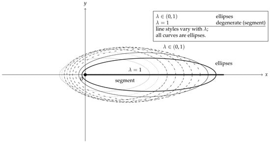
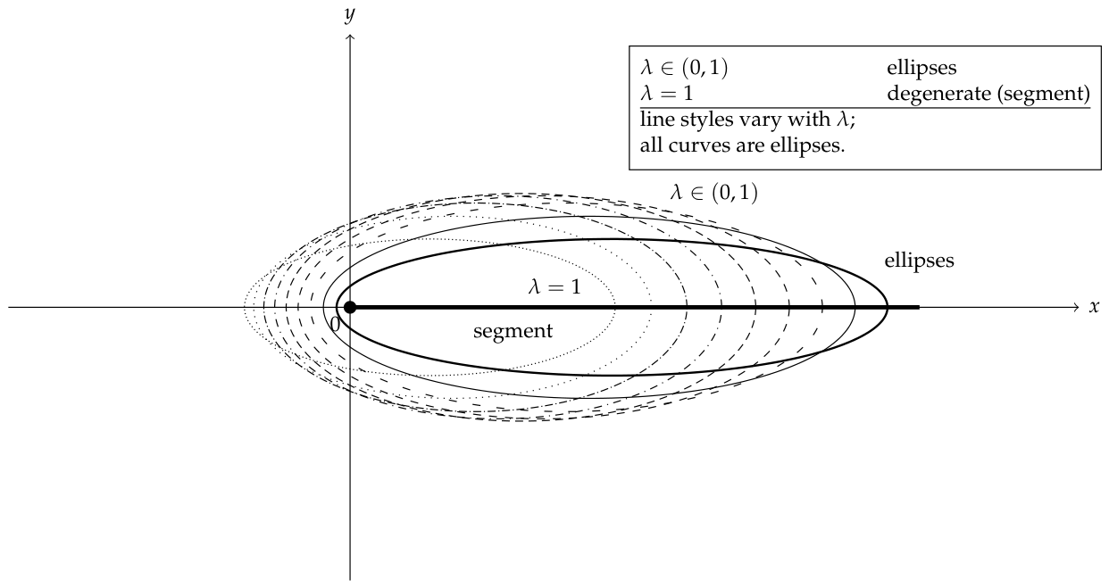
Figure 1 shows the family $\mathcal{E}\left(\lambda \right)$ for $\alpha =-0.5$ and $\beta =2$. For $\lambda \in (0,1)$, the curves are non-degenerate ellipses drawn with different line styles. At $\lambda =1$, the ellipse degenerates to a line segment, illustrating one of the degenerate cases described in Remark 1.

Figure 1. The family $\mathcal{E}\left(\lambda \right)$ for $\alpha =-0.5$, $\beta =2$. At $\lambda =1$ the ellipse degenerates to a line segment.

The following result shows that the support function of the ellipse $\mathcal{E}\left(\lambda \right)$ defined in Definition 1 coincides with that of the numerical range of the generalized pencil T.

Lemma 5.

For $\lambda \in [0,1]$, the support function of the ellipse $\mathcal{E}\left(\lambda \right)$ in Definition 1 is given by:

$${\rho }_{\mathcal{E}\left(\lambda \right)}\left(\theta \right)={\displaystyle \frac{1}{2}}\left[(1+\alpha +\beta \lambda )cos\theta +\sqrt{\left({(1+\alpha +\beta \lambda )}^2-4\alpha (1-\lambda )\right){cos}^2\theta +{\beta }^2\lambda (1-\lambda )}\right].$$

Proof. 

We proceed by distinguishing two cases.

Case (i): $\beta \ne 0$. If $\lambda \in (0,1)$, then by Remark 1 we have $a^2>0$ and $b^2>0$. Hence the boundary of $\mathcal{E}\left(\lambda \right)$ can be expressed in the quadratic form

$${(X-C)}^{\top }A(X-C)=1,$$

where

$$X=\left(\begin{array}{c}x\\ y\end{array}\right),C=\left(\begin{array}{c}c\\ 0\end{array}\right),A=\left(\begin{array}{cc}{a}^{-2}& 0\\ 0& b^{-2}\end{array}\right)$$

is positive definite. By [13], the support function of the compact convex set $\mathcal{E}\left(\lambda \right)$ is

$${\rho }_{\mathcal{E}\left(\lambda \right)}\left(\theta \right)=\underset{X\in \mathcal{E}\left(\lambda \right)}{sup}{d}^{\top }X,d=\left(\begin{array}{c}cos\theta \\ sin\theta \end{array}\right).$$

Since the supremum of a linear function over a compact convex set is attained on the boundary, it suffices to maximize $d^{\top }X$ subject to the boundary constraint ${(X-C)}^{\top }A(X-C)=1$. By Lemma 3, we form the Lagrangian

$$L(X,\mu )=d^{\top }X+\mu \left(1-{(X-C)}^{\top }A(X-C)\right),$$

and note that

$$d^{\top }X=xcos\theta +ysin\theta ,{(X-C)}^{\top }A(X-C)={\displaystyle \frac{{(x-c)}^2}{a^2}}+{\displaystyle \frac{y^2}{b^2}}.$$

Taking partial derivatives and setting them to zero yields

$${\displaystyle \frac{\partial L}{\partial x}}=cos\theta -2\mu {\displaystyle \frac{x-c}{a^2}}=0,{\displaystyle \frac{\partial L}{\partial y}}=sin\theta -2\mu {\displaystyle \frac{y}{b^2}}=0.$$

In vector form this reads

$$d-2\mu A(X-C)=0,$$

hence $d=2\mu A(X-C)$ and

$$X=C+{\displaystyle \frac{1}{2\mu }}{A}^{-1}d.$$

(7)

Substituting (7) into the constraint ${(X-C)}^{\top }A(X-C)=1$ gives

$${\displaystyle \frac{1}{4{\mu }^2}}{d}^{\top }{A}^{-1}d=1,$$

so that

$$\mu =\pm {\displaystyle \frac{1}{2}}\sqrt{d^{\top }{A}^{-1}d}.$$

Inserting these values of $\mu$ back into (7), we obtain two critical points

$$X=C\pm {\displaystyle \frac{A^{-1}d}{\sqrt{d^{\top }{A}^{-1}d}}}.$$

Evaluating the objective function at these critical points yields

$$d^{\top }X=d^{\top }C\pm \sqrt{d^{\top }{A}^{-1}d},$$

and the maximum is attained at the plus sign. Therefore,

$${\rho }_{\mathcal{E}\left(\lambda \right)}\left(\theta \right)=d^{\top }C+\sqrt{d^{\top }{A}^{-1}d}.$$

Substituting the explicit expressions for c, $a^2$, and $b^2$ given in Remark 1 into the right-hand side, we obtain

$${\rho }_{\mathcal{E}\left(\lambda \right)}\left(\theta \right)={\displaystyle \frac{1}{2}}\left[(1+\alpha +\beta \lambda )cos\theta +\sqrt{\left({(1+\alpha +\beta \lambda )}^2-4\alpha (1-\lambda )\right){cos}^2\theta +{\beta }^2\lambda (1-\lambda )}\right].$$

(8)

It remains to verify that (8) also holds at the endpoints of $[0,1]$.

For $\lambda =0$, Remark 1 shows that $\mathcal{E}\left(0\right)$ degenerates to the line segment $[c-a,c+a]$. Hence

$$\begin{array}{cc}\hfill {\rho }_{\mathcal{E}\left(0\right)}\left(\theta \right)& =\underset{x\in [c-a,c+a]}{sup}xcos\theta =ccos\theta +a|cos\theta |\hfill \\ & ={\displaystyle \frac{1}{2}}\left[(1+\alpha +\beta )cos\theta +\sqrt{\left({(1+\alpha +\beta )}^2-4\alpha \right){cos}^2\theta }\right].\hfill \end{array}$$

Setting $\lambda =0$ in (8) reduces to the same expression.

For $\lambda =1$, Remark 1 distinguishes two subcases. If $1+\alpha +\beta =0$, then $\mathcal{E}\left(1\right)$ degenerates to a point, and both the direct computation and (8) give ${\rho }_{\mathcal{E}\left(1\right)}\left(\theta \right)=0$. If $1+\alpha +\beta \ne 0$, then $\mathcal{E}\left(1\right)$ degenerates to the line segment $[c-a,c+a]$, and a computation analogous to the case $\lambda =0$ shows that its support function also agrees with (8).

Case (ii): $2=0$. In this case, Remark 1 shows that $\mathcal{E}\left(\lambda \right)$ degenerates to a line segment for every $\lambda \in [0,1]$, and an analogous direct computation confirms that its support function is still given by (8).

Having verified (8) for $\lambda \in (0,1)$ in the non-degenerate case, for the endpoints $\lambda =0,1$, and for the degenerate case $\beta =0$, we conclude that for every $\lambda \in [0,1]$,

$${\rho }_{\mathcal{E}\left(\lambda \right)}\left(\theta \right)={\displaystyle \frac{1}{2}}\left[(1+\alpha +\beta \lambda )cos\theta +\sqrt{\left({(1+\alpha +\beta \lambda )}^2-4\alpha (1-\lambda )\right){cos}^2\theta +{\beta }^2\lambda (1-\lambda )}\right].$$

□

We thus obtain the following explicit characterization of the closure of the numerical range of the generalized pencil T.

Proof of Theorem 2.

From Lemmas 4 and 5, we have

$$\begin{array}{cc}\hfill {\rho }_{W\left(T\right)}\left(\theta \right)& =\underset{\lambda \in \sigma \left(PQ\right)\setminus \left\{0\right\}}{sup}{\displaystyle \frac{1}{2}}\left[(1+\alpha +\beta \lambda )cos\theta +\sqrt{\left[{(1+\alpha +\beta \lambda )}^2-4\alpha (1-\lambda )\right]{cos}^2\theta +{\beta }^2\lambda (1-\lambda )}\right],\hfill \\ \hfill & =\underset{\lambda \in \sigma \left(PQ\right)\setminus \left\{0\right\}}{sup}{\rho }_{\mathcal{E}\left(\lambda \right)}\left(\theta \right).\hfill \end{array}$$

By Lemma 2, the support function of a convex hull of a family of sets equals the supremum of their individual support functions. Hence,

$$\overline{W\left(T\right)}=\overline{\mathrm{conv}\left\{{\cup }_{\lambda \in \sigma \left(PQ\right)\setminus \left\{0\right\}}\mathcal{E}\left(\lambda \right)\right\}}.$$

□

Combining Theorem 2 with the decomposition (1), we obtain the main result for the general case.

Proof of Theorem 1.

From the matrix form in (2), we have

$$P+\alpha Q+\beta PQ\sim (1+\alpha +\beta )I\oplus I\oplus \alpha I\oplus 0\oplus \left(\begin{array}{cc}1+(\alpha +\beta ){cos}^2{T}_0& (\alpha +\beta )cos{T}_{0}sin{T}_0\\ \alpha cos{T}_{0}sin{T}_0& \alpha {sin}^2{T}_0\end{array}\right).$$

Suppose $\tilde{\mathcal{H}}\ne \left\{0\right\}$. We consider the four intersection subspaces in turn.

(i)

If ${\mathcal{L}}^{\perp }\cap {\mathcal{N}}^{\perp }\ne \left\{0\right\}$, then $T=0$ on ${\mathcal{L}}^{\perp }\cap {\mathcal{N}}^{\perp }$. Hence on $({\mathcal{L}}^{\perp }\cap {\mathcal{N}}^{\perp })\oplus \tilde{\mathcal{H}}$ we obtain

$$\mathrm{conv}\left\{\right\{0\}\cup \overline{\mathrm{conv}\left\{{\cup }_{\lambda \in \sigma \left(PQ\right)\setminus \left\{0\right\}}\mathcal{E}\left(\lambda \right)\right\}}\}.$$

Since $\left\{0\right\}\subset \mathcal{E}\left(\lambda \right)$ for all $\lambda \in (0,1]$, the set $\left\{0\right\}$ is already contained in the convex hull of the ellipses. Therefore

$$\overline{W\left(T\right)}=\overline{\mathrm{conv}\left\{{\cup }_{\lambda \in \sigma \left(PQ\right)\setminus \left\{0\right\}}\mathcal{E}\left(\lambda \right)\right\}}$$

on the space ${\mathcal{L}}^{\perp }\cap {\mathcal{N}}^{\perp }\oplus \tilde{\mathcal{H}}$.

(ii)

If ${\mathcal{L}}^{\perp }\cap \mathcal{N}\ne \left\{0\right\}$, then $T=\alpha I$ on ${\mathcal{L}}^{\perp }\cap \mathcal{N}$. Hence on $({\mathcal{L}}^{\perp }\cap \mathcal{N})\oplus \tilde{\mathcal{H}}$ we obtain

$$\mathrm{conv}\left\{\right\{\alpha \}\cup \overline{\mathrm{conv}\left\{{\cup }_{\lambda \in \sigma \left(PQ\right)\setminus \left\{0\right\}}\mathcal{E}\left(\lambda \right)\right\}}\}.$$

Since $\alpha \le 0$, $\alpha +\beta \ge 0$, and $0\in \sigma \left(T_0\right)$, we have $\left\{1\right\}\subset \mathcal{E}\left(1\right)$. Because $\tilde{\mathcal{H}}\ne \left\{0\right\}$, the segment $[-0.5,1]$ is contained in $\overline{W\left(T\right)}$ on this subspace. Consequently,

$$\mathrm{conv}\{[\alpha ,1]\cup \overline{\mathrm{conv}\left\{{\cup }_{\lambda \in \sigma \left(PQ\right)\setminus \left\{0\right\}}\mathcal{E}\left(\lambda \right)\right\}}\}.$$

Under our assumptions, $\mathcal{E}\left(0\right)=[\alpha ,1]$ and $0\in \sigma \left(PQ\right)$. Thus

$$\overline{W\left(T\right)}=\mathrm{conv}\{\mathcal{E}\left(0\right)\cup \overline{\mathrm{conv}\left\{{\cup }_{\lambda \in \sigma \left(PQ\right)\setminus \left\{0\right\}}\mathcal{E}\left(\lambda \right)\right\}}\}=\overline{\mathrm{conv}\left\{{\cup }_{\lambda \in \sigma \left(PQ\right)}\mathcal{E}\left(\lambda \right)\right\}}$$

on the space $({\mathcal{L}}^{\perp }\cap \mathcal{N})\oplus \tilde{\mathcal{H}}$.

(iii)

If $\mathcal{L}\cap {\mathcal{N}}^{\perp }\ne \left\{0\right\}$, then $T=I$ on $\mathcal{L}\cap {\mathcal{N}}^{\perp }$. Hence on $(\mathcal{L}\cap {\mathcal{N}}^{\perp })\oplus \tilde{\mathcal{H}}$,

$$\mathrm{conv}\left\{\right\{1\}\cup \overline{\mathrm{conv}\left\{{\cup }_{\lambda \in \sigma \left(PQ\right)\setminus \left\{0\right\}}\mathcal{E}\left(\lambda \right)\right\}}\}.$$

Since $\left\{1\right\}\subset \mathcal{E}\left(1\right)$, the point 1 already belongs to the convex hull of the ellipses. Therefore

$$\overline{W\left(T\right)}=\overline{\mathrm{conv}\left\{{\cup }_{\lambda \in \sigma \left(PQ\right)\setminus \left\{0\right\}}\mathcal{E}\left(\lambda \right)\right\}}$$

on the space $(\mathcal{L}\cap {\mathcal{N}}^{\perp })\oplus \tilde{\mathcal{H}}$.

(iv)

If $\mathcal{L}\cap \mathcal{N}\ne \left\{0\right\}$, then $T=(1+\alpha +\beta )I$ on $\mathcal{L}\cap \mathcal{N}$. Hence on $(\mathcal{L}\cap \mathcal{N})\oplus \tilde{\mathcal{H}}$,

$$\mathrm{conv}\left\{\right\{(1+\alpha +\beta )\}\cup \overline{\mathrm{conv}\left\{{\cup }_{\lambda \in \sigma \left(PQ\right)\setminus \left\{0\right\}}\mathcal{E}\left(\lambda \right)\right\}}\}.$$

Since $\alpha +\beta \ge 0$, the segment $[0,1+\alpha +\beta ]$ is contained in $\overline{W\left(T\right)}$ on this subspace. Because $1\in \sigma \left(PQ\right)$ and, under our assumptions, $\mathcal{E}\left(1\right)=[0,1+\alpha +\beta ]$, we obtain

$$\overline{W\left(T\right)}=\mathrm{conv}\{\mathcal{E}\left(1\right)\cup \overline{\mathrm{conv}\left\{{\cup }_{\lambda \in \sigma \left(PQ\right)\setminus \left\{0\right\}}\mathcal{E}\left(\lambda \right)\right\}}\}=\overline{\mathrm{conv}\left\{{\cup }_{\lambda \in \sigma \left(PQ\right)\setminus \left\{0\right\}}\mathcal{E}\left(\lambda \right)\right\}}$$

on the space $(\mathcal{L}\cap \mathcal{N})\oplus \tilde{\mathcal{H}}$.

If several of these subspaces are simultaneously nontrivial, their scalar contributions combine within the convex hull and are already accounted for by the degenerate ellipses $\mathcal{E}\left(0\right)$ or $\mathcal{E}\left(1\right)$, as shown in the four cases above. Hence, under our assumptions, we arrive at the following dichotomy.

(a)

If ${\mathcal{L}}^{\perp }\cap \mathcal{N}\ne \left\{0\right\}$, then

$$\overline{W\left(T\right)}=\overline{\mathrm{conv}\left\{{\cup }_{\lambda \in \sigma \left(PQ\right)}\mathcal{E}\left(\lambda \right)\right\}}.$$

(b)

If ${\mathcal{L}}^{\perp }\cap \mathcal{N}=\left\{0\right\}$, then

$$\overline{W\left(T\right)}=\overline{\mathrm{conv}\left\{{\cup }_{\lambda \in \sigma \left(PQ\right)\setminus \left\{0\right\}}\mathcal{E}\left(\lambda \right)\right\}}.$$

□

Corollary 1.

Let T be the generalized pencil of a pair $(P,Q)$ of projections at $(\alpha ,\beta )\in {\mathbb{R}}^2$. If $\tilde{\mathcal{H}}=0$ and $\alpha \le 0$, then the closure of the numerical range of T is the closed convex hull of the family of ellipses $\mathcal{E}\left(\lambda \right)$ for $\lambda \in \sigma \left(PQ\right)$, under any of the following six conditions

(i) 

$\mathcal{L}\cap \mathcal{N}$, $\mathcal{L}\cap {\mathcal{N}}^{\perp }$, ${\mathcal{L}}^{\perp }\cap \mathcal{N}$ are all nontrivial.

(ii) 

$\mathcal{L}\cap \mathcal{N}=\left\{0\right\}$, while $\mathcal{L}\cap {\mathcal{N}}^{\perp }$, ${\mathcal{L}}^{\perp }\cap \mathcal{N}$, and ${\mathcal{L}}^{\perp }\cap {\mathcal{N}}^{\perp }$ are all nontrivial.

(iii) 

$\mathcal{L}\cap {\mathcal{N}}^{\perp }=\left\{0\right\}$, while $\mathcal{L}\cap \mathcal{N}$ and ${\mathcal{L}}^{\perp }\cap \mathcal{N}$ are nontrivial, and $1+\alpha +\beta \ge 1$.

(iv) 

${\mathcal{L}}^{\perp }\cap \mathcal{N}=\left\{0\right\}$, while $\mathcal{L}\cap \mathcal{N}$ and $\mathcal{L}\cap {\mathcal{N}}^{\perp }$ are nontrivial, and $\alpha =0$.

(v) 

$\mathcal{L}\cap \mathcal{N}\ne \left\{0\right\}$, while $\mathcal{L}\cap {\mathcal{N}}^{\perp }=\left\{0\right\}$ and ${\mathcal{L}}^{\perp }\cap \mathcal{N}=\left\{0\right\}$, and $\alpha =0$, $1+\alpha +\beta \ge 1$.

(vi) 

$\mathcal{L}\cap {\mathcal{N}}^{\perp }\ne \left\{0\right\}$, while $\mathcal{L}\cap \mathcal{N}=\left\{0\right\}$ and ${\mathcal{L}}^{\perp }\cap \mathcal{N}=\left\{0\right\}$, and $\alpha =0$.

Proof. 

When $\tilde{\mathcal{H}}=0$, from the matrix form in (4), we have

$$P+\alpha Q+\beta PQ\sim (1+\alpha +\beta )I\oplus I\oplus \alpha I\oplus 0.$$

Suppose condition (i) holds. Then $W\left(T\right)=W\left(\right(1+\alpha +\beta )I\oplus I\oplus \alpha I)=\mathrm{conv}\left\{\right\{1\}\cup \{\alpha \}\cup \{1+\alpha +\beta \left\}\right\}$. If $1+\alpha +\beta \ge 1$, then $W\left(T\right)=[\alpha ,1+\alpha +\beta ]$. In this case $\lambda \in \sigma \left(PQ\right)=\{0,1\}$, with $\mathcal{E}\left(0\right)=[\alpha ,1]$ and $\mathcal{E}\left(1\right)=[0,1+\alpha +\beta ]$, hence $W\left(T\right)=\mathrm{conv}\left\{\mathcal{E}\right(0)\cup \mathcal{E}(1\left)\right\}$. If $0\le 1+\alpha +\beta <1$ or $1+\alpha +\beta <0$, the conclusion follows similarly.

Now suppose condition (ii) holds. Since ${\mathcal{L}}^{\perp }\cap {\mathcal{N}}^{\perp }\ne \left\{0\right\}$ in this case, we have $W\left(T\right)=W(0\oplus I\oplus \alpha I)=\mathrm{conv}\left\{\right\{0\}\cup \{1\}\cup \{\alpha \left\}\right\}=[\alpha ,1]$. Here $\lambda \in \sigma \left(PQ\right)=\left\{0\right\}$, and since $\mathcal{E}\left(0\right)=[\alpha ,1]$, we obtain $W\left(T\right)=\mathcal{E}\left(0\right)$.

The remaining four conditions follow by analogous arguments; we omit the routine details. □

Corollary 2.

Let T be the generalized pencil of a pair $(P,Q)$ of projections at $(\alpha ,\beta )\in {\mathbb{R}}^2$. If $\alpha \le 0$, $\alpha +\beta \ge 0$, and $0\in \sigma \left(T_0\right)$, where $T_0$ is the self-adjoint operator appearing in (3), then

$$\overline{W\left(T\right)}=\overline{\mathrm{conv}\left\{{\cup }_{\lambda \in \sigma \left(PQ\right)\setminus \left\{0\right\}}\mathcal{E}\left(\lambda \right)\right\}}\subseteq \overline{\mathrm{conv}\left\{{\cup }_{\lambda \in [0,1]}\mathcal{E}\left(\lambda \right)\right\}}.$$

In particular, when ${\mathcal{L}}^{\perp }\cap \mathcal{N}\ne \left\{0\right\}$ and $\sigma \left(PQ\right)=[0,1]$,

$$\overline{W\left(T\right)}=\overline{\mathrm{conv}\left\{{\cup }_{\lambda \in [0,1]}\mathcal{E}\left(\lambda \right)\right\}}.$$

Proof. 

By Theorem 1 and the inclusion $\sigma \left(PQ\right)\subseteq [0,1]$, the result follows directly. □

3. Geometric Relations Between the Spectrum and the Numerical Range of Generalized Pencils

While Section 2 characterized the closure of the numerical range of the generalized pencil T in terms of the spectrum $\sigma \left(PQ\right)$, this section examines the geometric relationship between the closure of the numerical range of T and $\sigma \left(PQ\right)$. As shown in Section 2, under suitable assumptions, this closure coincides with the closed convex hull of a family of ellipses, i.e.,

$$\overline{W\left(T\right)}=\overline{\mathrm{conv}\left\{{\cup }_{\lambda \in \sigma \left(PQ\right)\setminus \left\{0\right\}}\mathcal{E}\left(\lambda \right)\right\}}.$$

From Definition 1, the set of all foci of the ellipses in this family is given by

$$\mathcal{F}=\left\{{\displaystyle \frac{1+\alpha +\beta \lambda \pm \sqrt{{(1+\alpha +\beta \lambda )}^2-4\alpha (1-\lambda )}}{2}}:\lambda \in \sigma \left(PQ\right)\setminus \left\{0\right\}\right\}.$$

we define the extended set ${\mathcal{F}}^{\prime }$ by allowing $\lambda$ to range over the full spectrum $\sigma \left(PQ\right)$.

Theorem 3.

Let $(P,Q)$ be a regular pair of projections, and let T be the generalized pencil of a pair $(P,Q)$ of projections at $(\alpha ,\beta )\in {\mathbb{R}}^2$. If $\alpha \le 0$, then

$$\overline{W\left(T\right)}=\overline{\mathrm{conv}\left\{{\cup }_{\lambda \in \sigma \left(PQ\right)\setminus \left\{0\right\}}\mathcal{E}\left(\lambda \right)\right\}},$$

and the spectrum of T coincides with the set of all foci of the ellipses in this family, i.e.,

$$\sigma \left(T\right)=\mathcal{F}.$$

Proof. 

From (3) we have the unitary equivalence

$$T\sim \left(\begin{array}{cc}1+(\alpha +\beta ){cos}^2{T}_0& (\alpha +\beta )cos{T}_{0}sin{T}_0\\ \alpha cos{T}_{0}sin{T}_0& \alpha {sin}^2{T}_0\end{array}\right).$$

Denote the operator matrix on the right-hand side by A. Set $H={sin}^2{T}_0$; then $I-H={cos}^2{T}_0$ and $0\le H\le I$ with $KerH=Ker(I-H)=\left\{0\right\}$. With $W=\sqrt{H(I-H)}$, the operator matrix A can be rewritten as

$$A=\left(\begin{array}{cc}1+(\alpha +\beta )(I-H)& (\alpha +\beta )W\\ \alpha W& \alpha H\end{array}\right).$$

All four entries of A are continuous functions of the self-adjoint operator H, hence they commute pairwise. For a $2\times 2$ operator matrix with commuting entries, invertibility is equivalent to the invertibility of its operator determinant. The operator determinant of $A-\lambda I$ is

$$\begin{array}{cc}\hfill Det(A-\lambda I)& =\left(1+(\alpha +\beta )(I-H)-\lambda I\right)(\alpha H-\lambda I)-\alpha (\alpha +\beta )W^2\hfill \\ & =\left((1+\alpha +\beta -\lambda )I-(\alpha +\beta )H\right)(\alpha H-\lambda I)-\alpha (\alpha +\beta )H(I-H).\hfill \end{array}$$

Since all factors commute, we may expand this in the same way as scalar polynomials. Using H as the variable, we obtain after simplification

$$Det(A-\lambda I)=(\alpha +\beta \lambda )H-(1+\alpha +\beta -\lambda )\lambda I.$$

Observe that $Det(A-\lambda I)$ is a continuous function of H, namely $g\left(H\right)$ with

$$g\left(x\right)=-({\lambda }^2-(1+\alpha +\beta -\beta x)\lambda +\alpha x),x\in \sigma \left(H\right).$$

By the spectral mapping property (iv) of the Borel functional calculus and continuity of g, $Det(A-\lambda I)$ is invertible if and only if $g\left(x\right)\ne 0$ for all $x\in \sigma \left(H\right)$. Thus, $\lambda \in \sigma \left(A\right)$ precisely when $det\left(A\right(x)-\lambda I)=0$ for some $x\in \sigma \left(H\right)$, where

$$A\left(x\right)=\left(\begin{array}{cc}1+(\alpha +\beta )(1-x)& (\alpha +\beta )\sqrt{x(1-x)}\\ \alpha \sqrt{x(1-x)}& \alpha x\end{array}\right).$$

A direct computation of the characteristic polynomial gives

$$\lambda ={\displaystyle \frac{1+\alpha +\beta -\beta x\pm \sqrt{{(1+\alpha +\beta -\beta x)}^2-4\alpha x}}{2}},x\in \sigma \left(H\right).$$

Rewrite (9) in terms of $y=1-x\in \sigma (I-H)$:

$$\lambda ={\displaystyle \frac{1+\alpha +\beta y\pm \sqrt{{(1+\alpha +\beta y)}^2-4\alpha (1-y)}}{2}},y\in \sigma (I-H).$$

Using $\sigma \left(PQP\right)=\sigma \left({cos}^2{T}_0\right)\cup \left\{0\right\}=\sigma (I-H)\cup \left\{0\right\}$ and $\sigma \left(PQP\right)\setminus \left\{0\right\}=\sigma \left(PQ\right)\setminus \left\{0\right\}$, we obtain $\sigma (I-H)\setminus \left\{0\right\}=\sigma \left(PQ\right)\setminus \left\{0\right\}$. Since 0 is not an eigenvalue of $I-H$, it can be removed without affecting the validity of (10); therefore

$$\sigma \left(T\right)=\left\{{\displaystyle \frac{1+\alpha +\beta \lambda \pm \sqrt{{(1+\alpha +\beta \lambda )}^2-4\alpha (1-\lambda )}}{2}},\lambda \in \sigma \left(PQ\right)\setminus \left\{0\right\}\right\}.$$

In this case Theorem 2 yields

$$\overline{W\left(T\right)}=\overline{\mathrm{conv}\left\{{\cup }_{\lambda \in \sigma \left(PQ\right)\setminus \left\{0\right\}}\mathcal{E}\left(\lambda \right)\right\}}.$$

From Definition 1, the set of all foci of the ellipses $\mathcal{E}\left(\lambda \right)$ for $\lambda \in \sigma \left(PQ\right)\setminus \left\{0\right\}$ in this family is

$$\mathcal{F}=\left\{{\displaystyle \frac{1+\alpha +\beta \lambda \pm \sqrt{{(1+\alpha +\beta \lambda )}^2-4\alpha (1-\lambda )}}{2}},\lambda \in \sigma \left(PQ\right)\setminus \left\{0\right\}\right\},$$

which is exactly the set on the right-hand side of (11).

Thus

$$\sigma \left(T\right)=\mathcal{F}.$$

Together with Theorem 2, this completes the proof. □

By Theorem 1, the result now extends to general pairs $(P,Q)$ of projections.

Theorem 4.

Let T be the generalized pencil of a pair $(P,Q)$ of projections at $(\alpha ,\beta )\in {\mathbb{R}}^2$, and assume that $\alpha \le 0$, $\alpha +\beta \ge 0$, and $0\in \sigma \left(T_0\right)$, where $T_0$ is the self-adjoint operator appearing in (3). Then Theorem 1 holds and we distinguish two cases.

(i) 

If ${\mathcal{L}}^{\perp }\cap \mathcal{N}\ne \left\{0\right\}$ and $\mathcal{L}\cap {\mathcal{N}}^{\perp }\ne \left\{0\right\}$, then

$$\sigma \left(T\right)={\mathcal{F}}^{\prime }.$$

(ii) 

If ${\mathcal{L}}^{\perp }\cap \mathcal{N}=\left\{0\right\}$ and $\mathcal{L}\cap {\mathcal{N}}^{\perp }=\left\{0\right\}$, then

$$\sigma \left(T\right)=\mathcal{F}.$$

Proof. 

From the matrix form in (2), we have

$$T\sim (1+\alpha +\beta )I\oplus I\oplus \alpha I\oplus 0\oplus \left(\begin{array}{cc}1+(\alpha +\beta ){cos}^2{T}_0& (\alpha +\beta )cos{T}_{0}sin{T}_0\\ \alpha cos{T}_{0}sin{T}_0& \alpha {sin}^2{T}_0\end{array}\right).$$

By Theorem 3, we have

$$\sigma \left(\tilde{T}\right)=\left\{{\displaystyle \frac{1+\alpha +\beta \lambda \pm \sqrt{{(1+\alpha +\beta \lambda )}^2-4\alpha (1-\lambda )}}{2}},\lambda \in \sigma \left(PQ\right)\setminus \left\{0\right\}\right\}.$$

The four intersection subspaces, if nontrivial, give the scalar eigenvalues

$$\sigma \left((1+\alpha +\beta )I\oplus I\oplus \alpha I\oplus 0\right)\subseteq \{1+\alpha +\beta ,1,\alpha ,0\}.$$

Therefore, the full spectrum of T is

$$\sigma \left(T\right)\subseteq \{1+\alpha +\beta ,1,\alpha ,0\}\cup \left\{{\displaystyle \frac{1+\alpha +\beta \lambda \pm \sqrt{{(1+\alpha +\beta \lambda )}^2-4\alpha (1-\lambda )}}{2}}:\lambda \in \sigma \left(PQ\right)\setminus \left\{0\right\}\right\}.$$

We now distinguish two cases.

Case (i): ${\mathcal{L}}^{\perp }\cap \mathcal{N}\ne \left\{0\right\}$ and $\mathcal{L}\cap {\mathcal{N}}^{\perp }\ne \left\{0\right\}$. On ${\mathcal{L}}^{\perp }\cap \mathcal{N}$ we have $T=\alpha I$, so $\alpha \in \sigma \left(T\right)$, and $PQ=0$, hence $0\in \sigma \left(PQ\right)$. On $\mathcal{L}\cap {\mathcal{N}}^{\perp }$ we have $T=I$, so $1\in \sigma \left(T\right)$. The hypothesis $0\in \sigma \left(T_0\right)$ gives $1\in \sigma \left(PQ\right)$. Since $\alpha +\beta \ge 0$, we have $\mathcal{E}\left(1\right)=[0,1+\alpha +\beta ]$, and by (12) at $\lambda =1$ the regular part $\tilde{T}$ contributes its two foci as spectral points. Since $0\in \sigma \left(PQ\right)$, the degenerate ellipse $\mathcal{E}\left(0\right)=[\alpha ,1]$ also enters the family, and its foci $\alpha$ and 1 coincide with the scalar eigenvalues coming from the two intersection subspaces. Therefore,

$$\sigma \left(T\right)={\mathcal{F}}^{\prime }.$$

Case (ii): ${\mathcal{L}}^{\perp }\cap \mathcal{N}=\left\{0\right\}$ and $\mathcal{L}\cap {\mathcal{N}}^{\perp }=\left\{0\right\}$. The scalar eigenvalues $\alpha$ and 1 are absent, and $\mathcal{E}\left(0\right)$ does not enter the family. Any remaining scalar contributions are already contained in the spectrum of the regular part. Therefore,

$$\sigma \left(T\right)=\mathcal{F}.$$

□

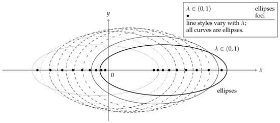
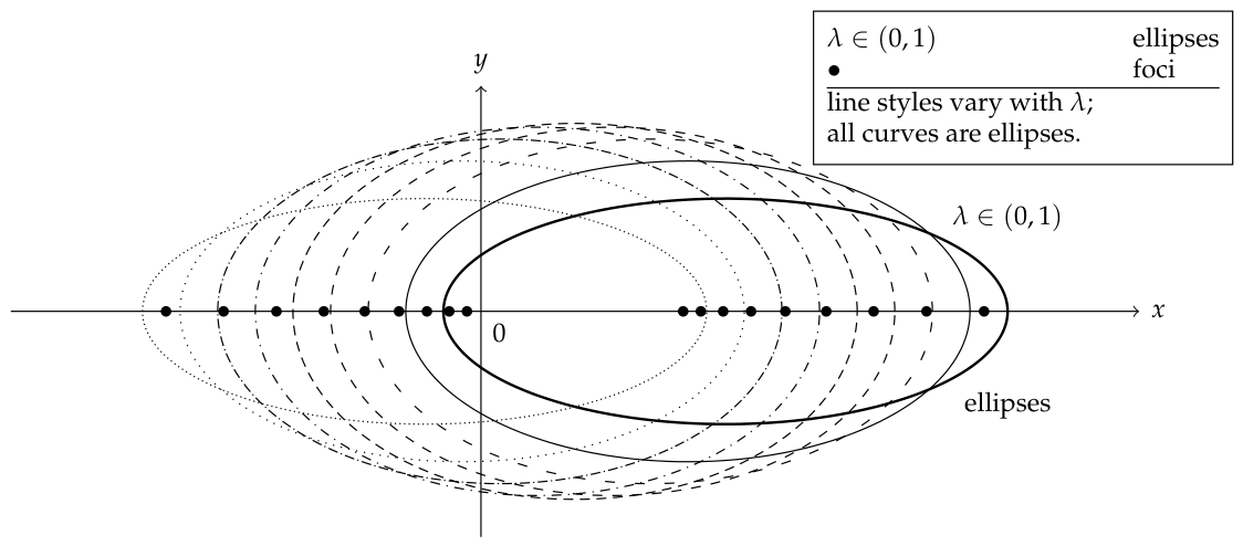
Theorem 3 (or Theorem 4) provides a clear geometric picture of how the spectrum $\sigma \left(T\right)$ sits inside the closure of the numerical range. Specifically, the spectrum $\sigma \left(T\right)$ coincides with the set of foci of the family of ellipses that characterize $\overline{W\left(T\right)}$, offering a precise geometric insight into the relationship between $\sigma \left(T\right)$ and $\overline{W\left(T\right)}$. Figure 2 shows several ellipses and the distribution of their foci.

Figure 2. The ellipses $\mathcal{E}\left(\lambda \right)$ for $\alpha =-2$, $\beta =4$. The black dots indicate the foci of each ellipse.

References

- Gustafson, K.E.; Rao, D.K.M. Numerical Range; Springer: New York, NY, USA, 1997. [Google Scholar]
- Chen, T.; Lai, W.N.; Deng, C.Y. Characterizations of generalized pencils of pairs of projections. Banach J. Math. Anal. 2024, 18, 11. [Google Scholar] [CrossRef] [Scilit]
- Markus, A.S. Introduction to the Spectral Theory of Polynomial Operator Pencils; American Mathematical Society: Providence, RI, USA, 1988. [Google Scholar]
- Cui, M.M.; Ji, G.X. Pencils of pairs of projections. Stud. Math. 2019, 249, 117–141. [Google Scholar] [CrossRef] [Scilit]
- Lai, W.N.; Chen, T.; Deng, C.Y. On the Generalized Pencils of Pairs of Projections. Acta Math. Sin. Chin. Ser. 2024, 67, 11. [Google Scholar]
- Yu, W.Y.; Wang, R.; Zhang, C. Geometric Characterization of the Numerical Range of Parallel Sum of Two Orthogonal Projections. J. Math. 2024, 2024, 1448498. [Google Scholar] [CrossRef] [Scilit]
- Zhang, C.; Yu, W.Y. The numerical range of the operator P + QP. J. Shangdong Univ. (Nat. Sci.) 2023, 58, 92–98. [Google Scholar]
- Halmos, P.R. Two subspaces. Trans. Am. Math. Soc. 1969, 144, 381–389. [Google Scholar] [CrossRef]
- Böttcher, A.; Spitkovsky, I.M. A gentle guide to the basics of two projections theory. Linear Algebra Its Appl. 2010, 432, 1412–1459. [Google Scholar] [CrossRef] [Scilit]
- Riesz, F.; Nagy, S.B. Functional Analysis; Dover Publications: New York, NY, USA, 1990. [Google Scholar]
- Conway, J.B. A Course in Functional Analysis, 2nd ed.; Springer: New York, NY, USA, 1989. [Google Scholar]
- Klaja, H. The numerical range and the spectrum of a product of two orthogonal projections. J. Math. Anal. Appl. 2014, 411, 177–195. [Google Scholar] [CrossRef] [Scilit]
- Rockafellar, R.T. Convex Analysis; Princeton University Press: Princeton, NJ, USA, 1970. [Google Scholar]
- Boyd, S.; Vandenberghe, L. Convex Optimization; Cambridge University Press: Cambridge, UK, 2004. [Google Scholar]
- Bertsekas, D.P. Constrained Optimization and Lagrange Multiplier Methods; Cambridge, MA, USA, 2014. [Google Scholar]
Disclaimer/Publisher’s Note: The statements, opinions and data contained in all publications are solely those of the individual author(s) and contributor(s) and not of MDPI and/or the editor(s). MDPI and/or the editor(s) disclaim responsibility for any injury to people or property resulting from any ideas, methods, instructions or products referred to in the content. |
© 2026 by the authors. Licensee MDPI, Basel, Switzerland. This article is an open access article distributed under the terms and conditions of the Creative Commons Attribution (CC BY) license.