


Abstract
Pitch control is the standard approach to regulating the rotational speed of large wind energy systems when the wind speed goes over its rated value. However, the pitch control system can also be used to reduce blade loads. In this last case, it is necessary to extend the classic collective pitch control system by including a complicated mechanism, which involves a Coleman or a Clarke transformation. This extension is known as the individual pitch control (IPC). While the performance of the IPC is satisfactory regarding the load alleviation, its dynamics remain insufficiently comprehended, especially due to the previously mentioned embedded transformations. Hence, the tuning of the IPC is sometimes challenging, and the controller can exhibit unexpected behaviours. The idea of this work is to formulate the IPC as a multivariable controller in the input/output representation such that the classic tools for the analysis and control of linear systems can be applied. As a result, some lesser-known properties as well as limitations are disclosed. Specifically, the approach makes apparent the existence of proportional-resonant controllers, which are crucial for dynamical behaviour. This additional knowledge can assist in the design of control systems and the tuning of controllers. A simulation study completes the presentation, including qualitative and quantitative analysis.
MSC:
93C35; 93C99
1. Introduction
Wind has always been an important source of energy, sometimes used directly through conversion into mechanical work, and more recently through extraction and conversion into electrical energy. That is the work carried out by modern wind turbines.
Over time, wind turbines have increased in size to meet an ever-growing demand for energy. This has led to the almost exclusive use of three-bladed machines with variable speed and variable pitch [1,2]. Consequently, the safety net and control systems have had to be improved to ensure safe and optimal operation in each of the different states in which the machine must be operated, which depend on wind speed [3,4].
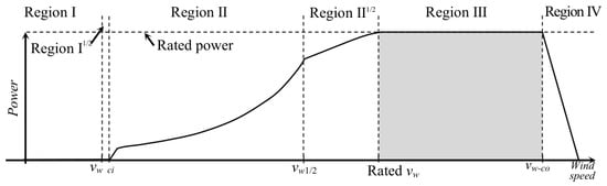
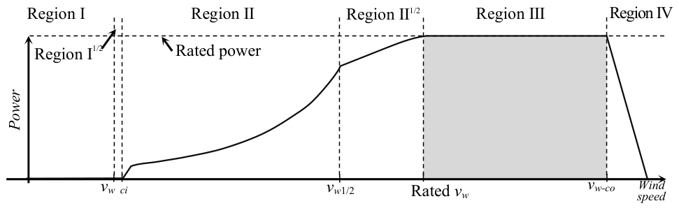
In particular, normally four discrete operational states can clearly be distinguished, which are associated with four operating regions. Each region has particular characteristics and requires different control strategies and configurations.
For a wind speed under the cut-in value, the wind energy converter cannot generate any power because the wind speed is very slow. This scenario is termed Region I. The second region (Region II), where the wind turbine produces energy without reaching the rated value, is determined by the range between cut-in and rated values. In this instance, there is a margin to maximise the energy conversion. The wind energy system moves to the third region (Region III) if the wind speed exceeds the rated value and remains there for wind speeds below the cut-out value. For all wind speeds in this region, the rotational speed must be regulated to the rated value in order to avoid damages and to maintain power generation at the specific design value of the machine. Finally, the wind turbine enters the fourth region (Region IV), where it must be shut down to preserve its structural health. The transition zones between Regions I and II, as well as Regions II and III, are often referred to as Regions I½ and II½, respectively. Figure 1 summarises the operational aspects previously described.
Figure 1.
Operational regions of a wind energy converter [4], where the region of interest is shadowed.
For the present contribution, the interest is focused on the third region, where a system for controlling blade pitch is such that the azimuthal rotational speed is maintained constantly despite the wind speed variations. The simplest approach is called collective pitch control (CPC) and is characterised by rotating the same pitch angle for all three blades [5]. However, the control objective for Region III should not necessarily be limited to the speed regulation. In addition to this, the pitch control system can also be used in order to reduce the loads acting on the blades. A review about pitch control in wind energy systems is provided, e.g., in [6].
Thus, both control objectives must simultaneously be satisfied by the pitch control system but, in this case, the CPC alone is insufficient. Therefore, the pitch angle delivered by the CPC for all the blades is individually corrected for each one by a second control mechanism. This mechanism is known as individual pitch control (IPC). The name refers to the individual fine adjustment of each pitch angle in relation to the collective pitch angle, rather than indicating a completely separate control for each blade, as the name might suggest. This procedure has been being developed and improved for more than 25 years. However, the focus has primarily been on the practical aspects and the capacity to alleviate blade loads, rather than figuring out the internal implications of the controller dynamics. The interest in the dynamic behaviour of the IPC has emerged more recently and is presented in seminal studies [7,8,9].
The IPC requires the measurements of all root bending moments of the blades and uses this information for the individual correction of the pitch angle of each blade. For further processing of this information, there are two approaches available in the literature: One that includes the transformation of the root bending moments and the corresponding inverse transformation of pitch angles, and the other that avoids using transformations at all. For the approach with transformations, there are also two possibilities. The classical and oldest approach was first proposed in [10] and later analysed, modified, and improved in [11]. It makes use of the Coleman transform, which was first used for the mechanical modelling of helicopters [12] and is mathematically identical to the Park transformation that is used in electrical systems. The Coleman transform converts the three root bending moments that are 120° out of phase with each other into two orthogonal moments.
The other approach, based on a transformation, was proposed about ten years later than the first one and uses the Clarke transformation [13]. The main difference between both is the fact that the Coleman transform requires the rotational angle, i.e., it is dynamic, while the Clarke transformation is a static one. Both approaches share the fact that they are based on multi-SISO control configurations (single input, single output).
The IPC can also be formulated as a fully coupled multivariable concept. Typical MIMO approaches based on LQG (linear–quadratic–Gaussian) can be found in [11,14,15]. IPC using the H∞ method is proposed in [16,17]. However, MIMO-IPC is not studied in the present work, since multi-SISO IPC configurations are at present the only ones of industrial interest, and are widely used.
On the other hand, despite its frequent use, the dynamics of the IPCs based on a multi-SISO configuration have still not been investigated in depth, particularly because they are overshadowed by transformations or by the reframing of the rotating parts into an inertial coordinate system, which complicates the study by using standard analysis tools.
In particular, multi-SISO IPCs are implemented with PI controllers in a rotating coordinate system. However, these PI controllers become proportional resonant controllers in an inertial coordinate system, which require different analyses and tunings. Moreover, it is not determined in the standard approaches if the IPCs have minimum phase dynamics or how the individual gains of each PI controller affect the overall IPC scheme.
On the other hand, a complete coupled multivariable controller that reveals the specific properties of the multi-SISO IPC mentioned above can be obtained by analytically substituting the transformations into the control system configurations.
Thus, this MIMO representation of the multi-SISO IPC is deduced in the current work, and its dynamic features are examined. The second section presents the classic IPC for the purpose of completeness. Finding the above-mentioned multivariable equivalent is the focus of Section 3, while the analysis with an example is the focus of Section 4. A simulation study is presented in Section 5, and finally, the conclusions are drawn in Section 6.
2. The IPC: Basic Formulation
2.1. General Aspects
The IPC was formulated with load reduction in mind. Although wind turbines may be subject to a variety of loads, which fall into five distinct groups (see [1]), the IPC is only focused on loads that arise from the periodic rotation of the wind turbine, or, to put it another way, at a frequency known as one per revolution (1P), which also corresponds to the rotor angular speed. Moreover, the IPC can also be used to reduce the higher harmonic components of the rotor speed, which are similarly significant and are typically denoted as 2P, 3P, …, nP.
According to Fourier analysis of the forces and moments, unsteady loads appear to be concentrated on the 1P, 2P, … frequency components [18]. In particular, fatigue loads that impact the hub, nacelle, tower, drivetrain, and blades can be found as 1P components [11]. The most significant impact on the non-rotary structure is provided by the 3kP fatigue load components (where k = 1, 2, …).
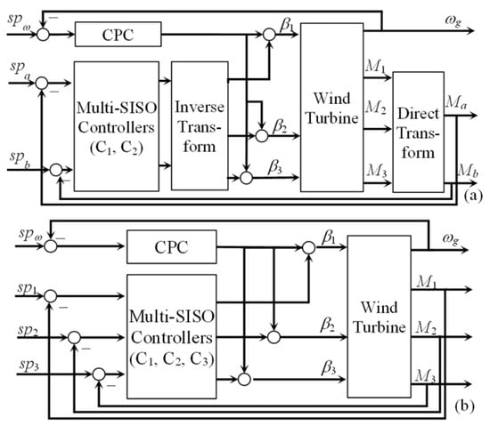
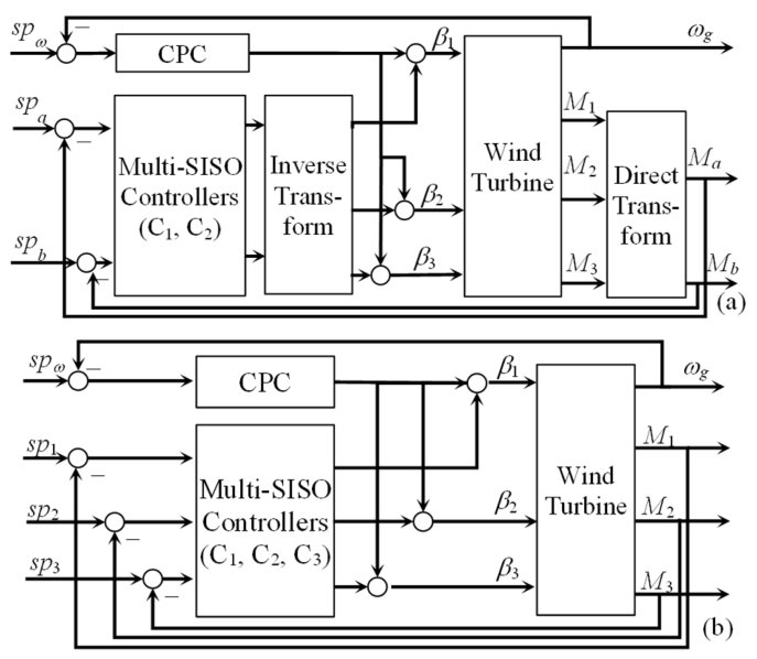
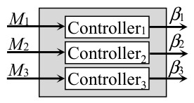
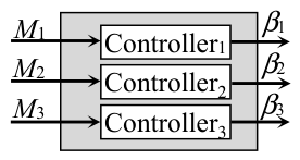
The control system configuration considers the three blade root bending moments as the output variables that are fed back to the controller, which provide the three pitch angle variations as control variables. Each variation is then individually added to the pitch angle supplied by the CPC to yield the correct angle for the pitch actuator of each blade. Hence, the control system implementation might include a transformation (see Figure 2a), or the transformation can be dispensed with, as shown in Figure 2b.
Figure 2.
IPC with transformation (a), without transformation (b).
It should be noted that the measured root bending moments require filtering. However, the dynamics of the filters are not included in the study to make the analysis more straightforward. The reference variables are set to zero, and PI control laws are used to implement the C1, C2, and C3 controllers referred to in Figure 2.
PI controllers can be configured in different ways (see, for instance, [19]). For this study it is necessary to have a controller whose parameters can be adjusted independently. This property is satisfied by the parallel non-interacting representation of a PI, whose transfer function is given by
2.2. Individual Pitch Control Based on the Coleman Transformation (Col-IPC)
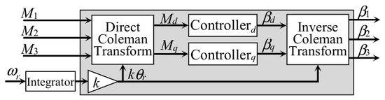
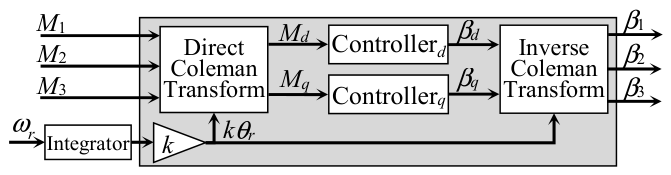
In the original IPC, the signals corresponding to the root bending moments are converted, using the Coleman transform, into two orthogonal moments (qd coordinate system). Hence, two controllers are placed in this dq coordinate system, with the transformed variables serving as feedback and zero set points. Finally, the control variables of both controllers are returned back to the initial coordinate system by means of the inverse Coleman transform.
In general, the k-th harmonic component of three variables that are coupled and phased 120 degrees apart can be Coleman transformed by using
where θr is the rotational angle. All the moments are described by the letter M. Moreover, number subscripts identify the variables in the original coordinated system, while the letter subscripts (d, q) denote the transformed variables. Variables generated in the rotating frame are transformed back by using the inverse Coleman transform expressed by
As a result, the block diagram depicted in Figure 3 represents the IPC, where the azimuthal angle is obtained by the integration of the rotational speed. PI controllers are the typically used in this scheme.
Figure 3.
Individual pitch control, including the Coleman transform.
2.3. Individual Pitch Control Based on the Clarke Transformation (Cla-IPC)
An important tool in the field of electrical engineering is the Clarke transform [20], also known as the αβγ transform. It is mainly used to simplify the design of control systems for three-phase inverters as well as the analysis of three-phase circuits. The transform becomes simpler when the system is balanced, and consequently, the component γ reduces to zero.
The design of an IPC on the basis of the Clarke transform is proposed in [13], adopting the name proportional-resonant IPC (PR-IPC). Since the Clarke transform takes place between two stationary coordinate systems, the outcome does not depend on the rotational angle, and this is its benefit. Although this approach has at present no industrial relevance, it is presented here for the sake of completeness and to show its similarities with the other approaches.
Proportional resonant controllers are more complex than the PI controller. The common equations for the Clarke transform are
for the forward way and
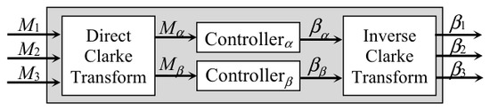
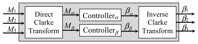
for the back way. The block diagram for the Cla-IPC is depicted in Figure 4.
Figure 4.
Individual pitch control, including the Clarke transform.
The proportional resonant controller is a PI controller translated to the αβ frame, whose transfer function is then given by
with ωr as the rotational frequency derived from the azimuthal speed.
2.4. Direct Individual Pitch Control (Without Any Transformation, Dia-IPC)
The direct IPC, i.e., an IPC that does not consider transformations, has been suggested in [21]. It implements a diagonal multi-SISO control topology that is called individual blade control (IBC). Additional references on the topic are [22,23].
The formulation assumes that the root bending moments are not coupled. Consequently, three independent PI controllers (one per blade) can be used, which result in a basic control scheme as shown in Figure 5. However, the PI controllers are expressed in a rotating coordinate system, and therefore should be reframed to an inertial coordinate system to carry out the analysis.
Figure 5.
Individual pitch control without any transformation.
3. IPC Described as a Multivariable Controller in Laplace Domain
The analysis of the individual pitch control system is challenging due to the existence of transformations. Hence, the way to simplify the mathematical treatment is by removing the transformations such that the controller is expressed as a transfer matrix with three inputs and three outputs. The development makes use of some concepts applied first in [7].
3.1. Col-IPC Formulated as Transfer Matrix
The derivation of the transfer matrix requires the assumption that the collective pitch controller is operating flawlessly. In such a case, the rotational speed is constant, which results in a rotational angle θr proportional to the time t, i.e., θr = ωr t, where ωr is the rotational frequency.
Combining the trigonometric angle addition and subtraction theorems and the above-mentioned assumption, (2) can be rewritten as
and it can also be reformulated as
The Laplace transforms of functions multiplied by time-dependent sines and cosines are given by
where j2 = −1, i.e., j is the imaginary unit. Hence, the Laplace transform of (8), taking into account (9), is expressed by
which can be rewritten in the vector form as
Matrix J* denotes the conjugated transpose of J. Moreover, J and L are defined by
respectively. M123 is the vector whose components are the Laplace-transformed moments M1, M2, and M3.
It has been practically observed [11,18] that the Coleman transform produces a phase shift within the transformed variables. Hence, the 1P, 2P, 4P, etc., harmonics in the fixed frame change to 0P, to 1P and 3P, to 3P and 5P, and so on, in the rotating frame. This characteristic is now analytically evident in (10) and (11).
It follows from Figure 3 that
where Mdq,ref are the references, and the PI controllers are defined by
It is also important to note that the references are zero and then
Following the same procedure in the output direction over the inverse Coleman transformation
the pitch angles are given by the vector
and considering (15), it can be written as
From (11), it follows that
such that (17) becomes
Since
(20) is then expressed as
or, reordering, also
The first product corresponds to
where Gc(s − jkωr) = Gcd(s − jkωr) + Gcq(s − jkωr), and the second product is
with Gc(s + jkωr) = Gcd(s + jkωr) + Gcq(s + jkωr). Adding both products, the bracket of (23) becomes
By shifting the variable s to s − jkωr and s + jkωr, the PI controllers are now rewritten as
with Kpc = Kpd + Kpq and Kic = Kid + Kiq. Hence, the addition and subtraction of the two equations yield
Thus, (26) becomes
whether (28) is introduced in (26). Finally, pre- and post-multiplying by LT and L, respectively, it follows
which, under consideration of (23), leads to the final control law given by
Several aspects that are typically concealed by the Coleman transform are revealed by the final equations. They are examined in the following section.
3.2. Cla-IPC Expressed as Transfer Matrix
When the Coleman transform is substituted with the Clarke one, the control system design confronts several difficulties. For example, the design does not consider harmonics 1P, 2P, …, and nP, and the controller works within a fixed frame while managing a rotating system. Accordingly, the PI controller needs to be reframed from the qd to the αβ coordinated system. The controller reframing can be done by using
as proposed in [24]. Hence, when (32) is applied to (1), it results in a controller whose control law is
It is referred to as an ideal proportional resonant (PR) controller. It should be pointed out that the transfer functions on the diagonal of (31) are PR controllers as well.
The transfer matrix of the Cla-IPC is obtained in the same way as the Col-IPC, but considering PR controllers and the Clarke transform instead of PI controllers and the Coleman transform, the result is expressed by
where
respectively.
3.3. Dia-IPC Expressed as Transfer Matrix
The IPC without transformation from Figure 5 is normally implemented as a transfer matrix with only PI controllers in the diagonal, namely
However, this case also consists of controllers for a fixed frame operating with a turning system. Therefore, the controllers should also be reframed by using (32). This leads to
4. Analysis of the IPC Dynamics
Several findings can be extracted from the transfer matrices (31), (34), and (36). These aspects are analysed in the ensuing subsections.
4.1. General Observations
Both the Coleman-transformed and Clarke-transformed IPC are fully coupled MIMO controllers. The IPC without transformation is completely decoupled. The assumption of decoupling or weak coupling that supports the IPC without transformations seems to be a very strong assertion. This may depend on the particular machine in question, and therefore, before implementation, the validity of the decoupling assumption should be examined for the different wind speeds of Region III.
Another observation is the fact that the diagonal elements of transfer matrices for the Col-IPC and Dia-IPC are filled with proportional resonant controllers. Moreover, all diagonal elements in the same transfer matrix are identical. The case of Cla-IPC is slightly more complex, but proportional resonant controllers are also present. Proportional resonant controllers have particular dynamics that require a separate analysis.
In the case of Col-IPC, the controller parameters in the elements of the transfer matrix are obtained by adding the parameters of both PI controllers, specifically, Kpc = Kpd + Kpq and Kic = Kid + Kiq. Hence, the individual consideration in the MIMO-IPC of each PI controller is non-sensitive because they produce a joint effect. Moreover, three elements of the Col-IPC transfer matrix might have zeros on the right side of the s-plane. This characteristic corresponds to the elements G12, G23, and G31.
That is, the angle of a given blade receives a negative contribution from its root bending moment. The root bending moment of the blade at 120° in front of the given blade contributes an angle affected by a zero that can be non-minimum phase, while the moment of the blade 120° behind the given blade contributes an angle affected by a minimum- phase zero.
Controllers with such characteristics are not necessarily problematic, but they can introduce some limitations, such as, for instance, a phase lag that reduces phase margin, a bandwidth limitation, and a slower reaction. For these reasons, the following analysis will focus on the necessary conditions for the controller parameters to avoid zeros on the right side.
According to the Routh–Hurwitz criterion [25], the condition for the second-order numerator of elements G12, G23, and G31 to have roots with negative real parts is that all coefficients are positive, namely,
The first condition requires that both parameters, Kpc and Kic, have the same sign. The second inequality, considering that k and ωr are positive, leads to
Finally, considering that Kpc = Kpd + Kpq and Kic = Kid + Kiq, it follows
The simplest case is to choose Kp = Kpd = Kpq and Ki = Kid = Kiq, which gives
where normally k = 1, 2, or 3. If the parameters of both controllers are chosen differently, then the condition can be expressed by
Thus, (41) and (42) can be used as constraints in the parametric optimisation to determine the controller parameters.
Finally, the root bending moment of a blade entering full-coupled MIMO controllers contributes positively to the corresponding pitch angle and negatively to the cross-pitch angles.
4.2. Analysis of the Controller Behaviour
This analysis is only for the Col-IPC, which is the most popular and widely utilised. However, similar studies can be performed for the other IPCs. The transfer matrix (31) is now brought into the form of
with Kc = Kic/Kpc, and . On the other hand, the characteristic equation is given by
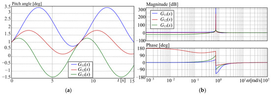
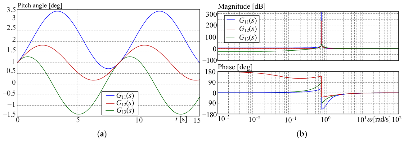
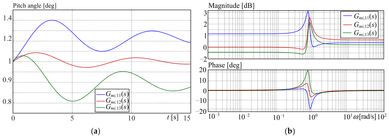
which means that the controller has two poles on the imaginary axis s1,2 = ±jkωr. That is, the controller as an isolated system has a step response with constant-amplitude oscillations, as depicted in Figure 6a.
Figure 6.
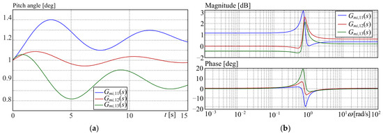
Analysis of G11, G12, and G13. (a) Step response, (b) Bode diagram.
For a better understanding of the controller behaviour, the following values are assigned to the parameters ωr = 0.7495 rad/s, Kpc = 1.3, Kic = 0.8, and k = 1. Thus, the poles are placed on s1,2 = ±j 0.7495, and the zeros are z1,2 = −0.6474 ± j 0.7631, z1,2 = 0.032 ± j 0.763, and z1,2 = −0.3077 ± j 0.6833 for G11(s), G12(s), and G13(s), respectively. Notice that the zeros of G12 are on the right half plane. The Bode diagrams of G11(s), G12(s), and G13(s) are depicted in Figure 6a.
4.3. Properties of Proportional Resonant Controllers
From the Bode diagram of Figure 6a, it is observable that proportional resonant controllers have a large amplitude peak at the rotating frequency. The objective is to reduce vibrations caused by mass imbalance and misalignment, as well as periodic moments. However, it can also lead to system instability [26].
Hence, if the MIMO-IPC is going to be implemented for real applications, the controller should be modified. Thus, one method to increase stability is to replace the integrator of the PI controller (1) in the rotation frame with a first-order filter, such that
where ωc is the cut frequency that determines the resonant peak width. When (32) is applied to (45), the PI changes in the stationary frame to
Moreover, if the condition ωc << ωr is met, the proportional resonant controller approximates
With this new controller (47), the diagonal elements of the transfer matrix (31) are
The non-diagonal elements of the transfer matrix can also be derived in the same manner, and the result is expressed by
For ωc = 0.1 rad/s, the poles move to s1,2 = −0.1± j 0.7428, and the zeros are locked now at z1,2 =−0.1308 ± j 0.7379, z1,2 =−0.1308 ± j 0.6962, and z1,2 =−0.1308 ± j 0.7774 for Gmi,11, Gmi,12, and Gmi,13, respectively. Figure 7 shows the step response and Bode diagram for the controller with the modified integrator.
Figure 7.
Analysis for the controller with a modified integrator. (a) Step response, (b) Bode diagram.
5. Numerical Study Based on Simulations
5.1. Reference Wind Turbine
The IPC formulated as a transfer matrix has been subject to a comparative study on the 20 MW reference wind turbine. The machine was proposed in [27]. Later, it was studied from the control point of view in [28]. Afterwards, it was parametrically modified and adjusted to guarantee compliance with OpenFAST 4.2.1 (previously referred to as FAST [29]). For the pitch control system, MATLAB/Simulink (R2025b) and the interface provided by OpenFAST are used.
The pertinent specs of the reference wind turbine are extracted from [28] and summarised in Table 1.
Table 1.
Relevant data of the 20 MW reference wind turbine.
5.2. Setup for Performing the Simulations
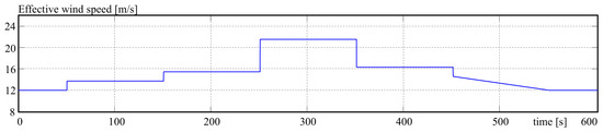
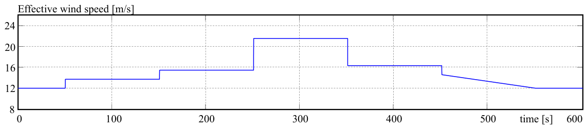
The reference wind energy converter is simulated using OpenFAST v. 4.2.1. In order to study the performance of the pitch control system, the machine is operated in Region III with a stepwise changing effective wind speed between 12 and 23 m/s perpendicular to the rotor, whose profile is depicted in Figure 8.
Figure 8.
Profile of the effective wind speed.
The solver has been configured with a fourth-order Adams–Bashforth–Moulton algorithm and an integration step of 0.0125 s. The initial conditions are set to the nominal operational conditions for Region III and the simulation time to 600 s. In addition, the root bending moments are notch-filtered for a rotational frequency of 0.7497 rad/s.
5.3. Control System Design
The subject of this work is individual pitch control. However, other control loops are essential for the normal operation of the wind turbine: for instance, the torque control and the collective pitch control. Thus, such control systems have to be included in the design in order to ensure the reproducibility of the experiments.
For the torque control, the classic optimal torque control (OTC), whose control law is given by
is used, and the collective pitch control system is implemented by using a PI controller with gain scheduling. All controller parameters are summarised in Table 2.
Table 2.
Controller parameters for all controllers.
It is important to mention here that the parameters for the proportional resonant controller are obtained as the sum of the parameters of the Col-IPC, i.e., Kpd + Kpq and Kid + Kiq. These two parameters are then used in all nine elements of the transfer matrix.
Notice that the parameters of the CPC are negative in order to satisfy the inverse proportionality characteristic of this control system, i.e., the rotational speed is reduced when the pitch angle is increased. Moreover, the root bending moments expressed in Nm are in the order of 105. For this reason, the integral gains of the controllers are consequently very small.
5.4. Simulation Results
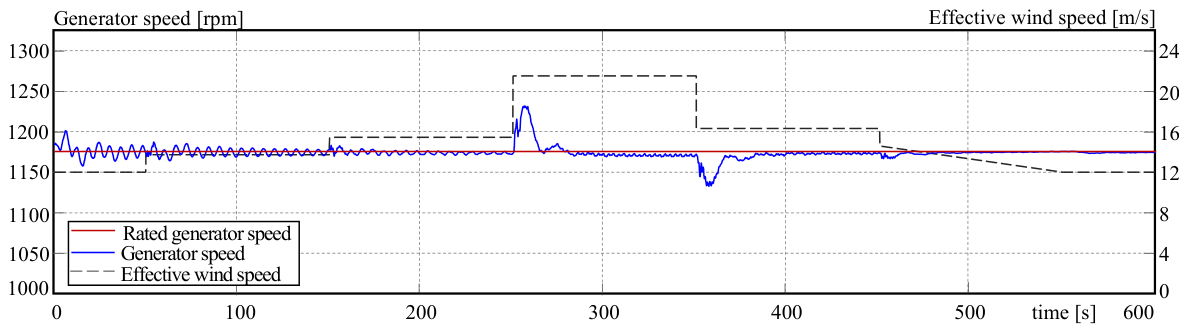
The duty of the individual pitch control system is not related to the regulation of the generator speed at its rated value. This is the task of the collective pitch control system. However, the validity of the development is based on the assumption that the wind turbine is operated under perfect collective pitch control. Thus, the first simulation experiment is to confirm that this requisite is satisfied. The regulation takes place at the rated value of 1173.7 rpm. The simulation is shown in Figure 9.
Figure 9.
Generator speed under the operation of the collective pitch controller.
Hence, the controller is able to maintain the generator speed around the nominal value with a ripple below 0.1%. There are only some deviations when the wind speed changes abruptly, but the differences are lower than 3.5%, and they are rapidly reduced by the controller. Hence, the CPC can be considered as working perfectly from a practical viewpoint.
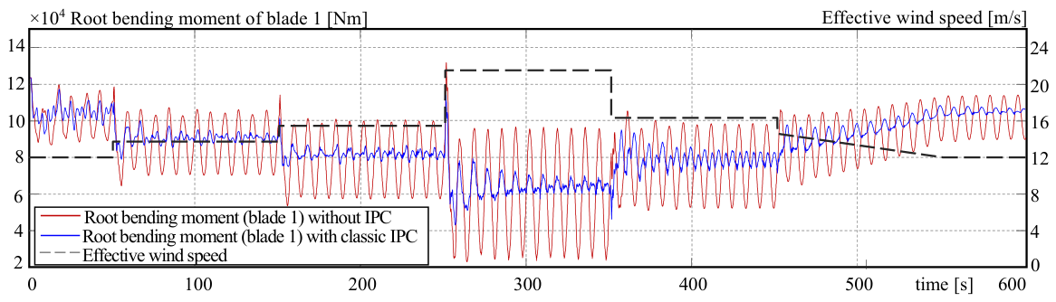
It is also important to confirm the correct operation of the IPC. This is done by contrasting the root bending moment of blade 1 without and with IPC. The IPC used is that which includes the Coleman transform. The result is depicted in Figure 10, where it is possible to appreciate the amplitude reduction in the root bending moment.
Figure 10.
Root bending moments in blade one, without and with IPC.
It should be remarked that the reference wind turbine has identical, balanced blades. Thus, only one blade is analysed because the others show similar results.
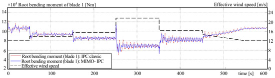
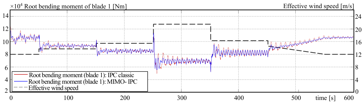
The next step is to verify whether the derived MIMO controller exhibits behaviour similar to that of the IPC with the Coleman transform. An important point to take into account is the fact that the MIMO controller is obtained under the assumption that the rotational speed is constant. However, although this is achieved because that is the task of the CPC, there are deviations around the rated value, particularly when there are abrupt changes in wind speed, as can be seen in Figure 9. Hence, it is necessary to analyse the impact of non-compliance with this condition on the differences with the original IPC. The result is presented in Figure 11.
Figure 11.
Root bending moments in blade 1, under Col-IPC and MIMO-IPC.
As it is possible to observe, the MIMO-IPC exhibits a response very similar to the Coleman IPC, and occasionally it even shows a greater attenuation of the amplitude of the root bending moments. This improvement is partly due to the elimination of the non-linearities as well as numeric approximations that are introduced when the calculation includes sine and cosine functions.
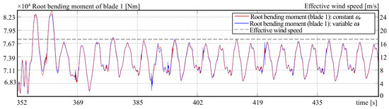
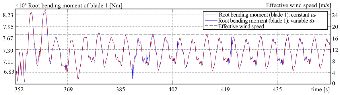
Another aspect to consider is the calculation using a constant rotational speed, which in this case was defined as ωr = 0.7497 rad/s. If the CPC is unable to reduce vibrations below a value for which the rotational speed can be assumed to be constant from a practical perspective, the approach can be improved by doing parameter adaptation. Since a measurement of the generator speed is available and the gearbox ratio is known, the instantaneous value of the rotational speed can be continuously recalculated, and with them, the controller parameters are adjusted. Although the CPC for this example has optimally been tuned, the adaptive approach was also implemented and tested. Results are illustrated in Figure 12.
Figure 12.
MIMO-IPC without and with parameter adaptation.
As the collective pitch control improves its performance, it becomes less necessary to adjust the controller parameters. Moreover, the variability of the rotational speed depends on the wind as well as machine dynamics. As mentioned above, since the CPC has optimised parameters in this example, the benefit of adaptation is smaller, as shown in Figure 12. However, the quantitative analysis in the following section clearly shows that it provides an improvement. Since the variability in rotational speed can increase at any time, it is advantageous to directly implement the adaptive approach.
5.5. Quantitative Analysis
To perform a quantitative comparison of the results produced by the different controllers, several parametric statistical measures are calculated. The most important ones are mean value (MV), standard deviation (SD), peak-to-peak value (P2P), root mean square (RMS) and crest factor (CF).
Based on the theoretical derivation as well as the qualitative analysis of the previous section, several premises can be formulated that should be confirmed by the quantitative analysis:
- -
- The amplitudes of the root bending moments should be considerably reduced as a consequence of adding the individual pitch control concept to the pitch control system. This is one of the reasons to complement the CPC with an IPC.
- -
- The MIMO-IPC is another mathematical representation of the IPC based on the Coleman transformation. However, it is derived assuming that the rotational speed is constant. Hence, if the rotational speed shows some variations, the results can differ from the results of the Coleman-IPC. On the other hand, the MIMO-IPC does not compute sine and cosine functions, which can affect the accuracy in the calculations. Consequently, this advantage can compensate for variations in the rotational speed.
- -
- The adaptive MIMO-IPC is designed to avoid the possible variations in the rotational speed. Thus, its results should be closer to the Coleman-IPC than to the MIMO-IPC. On the other hand, it does not compute sine and cosine functions, and therefore, it could potentially provide slightly better results than the Coleman-IPC.
The numeric calculations of the statistic measures for blade 1 are summarised in Table 3.
Table 3.
Quantitative parameters for blade 1.
The most remarkable improvement is observed between results without and with IPC for all parameters, showing the positive effect of the IPC on the root bending moments. The first premise is confirmed by the first two rows in the peak-to-peak (P2P) session of Table 3.
In order to study the second premise, the second and third rows of all sections of Table 3 are analysed. As the numbers are very similar, it can be concluded that both controllers have an equivalent behaviour. This result also indicates that the CPC performed sufficiently well that variations in the rotational speed are not numerically significant.
The last premise requires the analysis of the last three rows of each section of Table 3. This comparison shows that the most numbers of the adaptive MIMO-IPC are set between the Coleman-IPC and the MIMO-IPC. Moreover, the numbers of both MIMO-IPCs are slightly better than the Coleman-IPC. Since the second premise is satisfied, the improved differences of the MIMO-IPC can be attributed to its superior numerical properties.
6. Conclusions
The current study reformulates individual pitch control as a transfer matrix. This representation elucidates certain dynamic aspects of the controllers that would otherwise remain masked by the transformations. The newly revealed aspects are further examined.
For example, the frequency shifts observed experimentally in the Coleman IPC are now explicitly expressed in the analytical description. Moreover, the transfer matrix shows how the IPC dynamically affects the blade couplings through the pitch angles, with the possible appearance of non-minimal phase zeros. Another important finding is the fact that the PI controllers included in the standard IPC correspond to proportional resonant controllers in the stationary frame, whose properties differ from those of the classic PI. Thus, an analysis of the overall control system should consider PR controllers instead of PI controllers.
It was also verified by means of simulations that the derived MIMO-IPC performs very similarly to the Col-IPC, confirming the equivalence for the given scenario. In several situations, the MIMO-IPC performs even better than the Col-IPC because it offers better numerical properties. Hence, although it was first developed for analytical purposes, it can also be used for control because of its performance.
A deep comparison with the Clarke IPC and the diagonal IPC is not included in this work.; however, the topic is under study and will be part of work in the near future.
Funding
This research received no external funding.
Data Availability Statement
The raw data supporting the conclusions of this article will be made available by the authors on request if this is allowed by the academic institution.
Conflicts of Interest
The author declares no conflicts of interest. The funders had no role in the design of its study, in the collection, analyses, or interpretation of data, in the writing of the manuscript, or in the decision to publish these results.
Abbreviations
| CPC | Collective Pitch Control |
| IPC | Individual Pitch Control |
| LQG | Linear–Quadratic–Gaussian |
| MIMO | Multi Input, Multi Output |
| OTC | Optimal Torque Control |
| PI | Proportional Integral |
| PR | Proportional Resonant |
| SISO | Single Input, Single Output |
Nomenclature
| Parameters | |
| j | Imaginary unit, -- |
| k | Multiplicity that indicates the harmonic under consideration (1P, 2P, etc.) |
| Kp, Ki | Parameters of the PI controller |
| Kp1, Kp2, Kp3, Ki1, Ki2, Ki3 | Parameters of the three PI controllers |
| Kpd, Kpq, Kid, Kiq | Parameters of the PI controllers in the d and q axis |
| ωc | Cut frequency for the first order filter |
| Variables | |
| Β1, β2, β3, βα, ββ, βd, βq | Pitch angles, rad |
| β123, βdq, βαβ | Vectors of pitch angles, rad |
| M1, M2, M3, Mα, Mβ, Md, Mq | Roots bending moments, Nm |
| M123, Mdq, Mαβ | Vectors of roots bending moments, rad |
| sp1, sp2, sp3, spa, spb, spω | Set points for different control loops |
| t | Time |
| θg, θr | Generator rotational angle, rotor rotational angle, rad |
| ωg, ωr | Generator speed, rotor speed, rad/s |
| Functions | |
| f(t), F(s) | Generic function, and its Laplace transform |
| Gc(s) | Transfer matrix of the MIMO controller |
| Gc1 (s), Gc2 (s), Gc3 (s) | Transfer functions of controllers |
| Gαβ(s), Gdq(s), Gcα(s), Gcβ(s) | Transfer functions of controllers in the αβ- and dq-axis |
| Gpi(s), Gpr(s) | Transfer functions of PI and PR controllers |
References
- Manwell, J.F.; McGowan, J.G.; Ram, B. Wind Energy Explained: On Land and Offshore, 3rd ed.; John Wiley & Sons: Chichester, UK, 2024. [Google Scholar]
- Burton, T.; Jenkins, N.; Bossanyi, E.; Sharpe, D.; Graham, M. Wind Energy Handbook, 3rd ed.; John Wiley and Sons: Chichester, UK, 2021. [Google Scholar]
- Bianchi, F.D.; de Battista, H.; Mantz, R.J. Wind Turbine Control Systems; Springer: London, UK, 2007. [Google Scholar]
- Gambier, A. Control of Large Wind Energy Systems; Springer Nature: Basel, Switzerland, 2022. [Google Scholar]
- Bossanyi, E.A. The design of closed loop controllers for wind turbines. Wind Energy 2000, 3, 149–163. [Google Scholar] [CrossRef]
- Gambier, A. Pitch control of three bladed large wind energy converters—A Review. Energies 2021, 14, 8083. [Google Scholar] [CrossRef] [Scilit]
- Lu, Q.; Bowyer, R.; Jones, B.L. Analysis and design of Coleman transform-based individual pitch controllers for wind-turbine load reduction. Wind Energy 2015, 18, 1451–1468. [Google Scholar] [CrossRef] [Scilit]
- Lio, W.H.; Jones, B.L.; Lu, Q.; Rossiter, J.A. Fundamental performance similarities between individual pitch control strategies for wind turbines. Int. J. Control 2017, 90, 37–52. [Google Scholar] [CrossRef] [Scilit]
- Gambier, A. Multivariable representation and analysis of controllers used for individual pitch control of large wind energy converters. In Proceedings of the 22nd International Conference on Control, Automation and Systems (ICCAS), Jeju, Republic of Korea, 27 November–1 December 2022; pp. 403–408. [Google Scholar] [CrossRef] [Scilit]
- Caselitz, P.; Kleinkauf, W.; Krüger, T.; Petschenka, J.; Reichardt, M.; Störzel, K. Reduction of fatigue loads on wind energy converters by advanced control methods. In Proceedings of the European Wind Energy Conference, Dublin, Ireland, 8 October 1997; pp. 555–558. [Google Scholar]
- Bossanyi, E.A. Individual blade pitch control for load reduction. Wind Energy 2003, 6, 119–128. [Google Scholar] [CrossRef] [Scilit]
- Coleman, R.P.; Feingold, A.M. Theory of Self-Excited Mechanical Oscillations of Helicopter Rotors with Hinged Blades; Technical Notes; National Advisory Committee for Aeronautics: Langley, VA, USA, 1957. [Google Scholar]
- Zhang, Y.; Chen, Z.; Cheng, M. Proportional resonant individual pitch control for mitigation of wind turbines loads. IET Renew. Power Gener. 2013, 7, 191–200. [Google Scholar] [CrossRef] [Scilit]
- Stol, K.A.; Moll, H.-G.; Bir, G.; Namik, H. A comparison of multi-blade coordinate transformation and direct periodic techniques for wind turbine control design. In Proceedings of the 47th AIAA Aerospace Sciences Meeting, Orlando, FL, USA, 5–8 January 2009; pp. 1–10. [Google Scholar] [CrossRef] [Scilit]
- Selvam, K.; Kanev, S.; van Wingerden, J.W.; van Engelen, T.; Verhaegen, M. Feedback–feedforward individual pitch control for wind turbine load reduction. Int. J. Robust Nonlinear Control 2009, 19, 72–91. [Google Scholar] [CrossRef] [Scilit]
- Shan, M. Load Reducing Control for Wind Turbines; Fraunhofer Verlag: Stuttgart, Germany, 2017. [Google Scholar]
- Ungurán, R.; Petrovic, V.; Boersma, S.; van Wingerden, J.-W.; Pao, L.Y.; Kühn, M. Feedback-feedforward individual pitch control design for wind turbines with uncertain measurements. In Proceedings of the 2019 American Control Conference, Philadelphia, PA, USA, 10–12 July 2019; pp. 4151–4158. [Google Scholar] [CrossRef] [Scilit]
- Barlas, T.K.; van Kuik, G.A.M. Review of state of the art in smart rotor control research for wind turbines. Prog. Aerosp. Sci. 2009, 46, 1–27. [Google Scholar] [CrossRef] [Scilit]
- Visioli, A. Practical PID Control; Springer: London, UK, 2006. [Google Scholar]
- Duesterhoeft, W.C.; Schulz, M.W.; Clarke, E. Determination of instantaneous currents and voltages by means of alpha, beta, and zero components. Trans. Am. Inst. Electr. Eng. 1951, 70, 1248–1255. [Google Scholar] [CrossRef] [Scilit]
- Leithead, W.E.; Neilson, V.; Dominguez, S. Alleviation of unbalanced rotor loads by single blade controllers. In Proceedings of the Wind Energy Conference and Exhibition (EWEC), Marseille, France, 16–19 March 2009; pp. 1–9. [Google Scholar]
- Han, Y.; Leithead, W.E. Combined wind turbine fatigue and ultimate load reduction by individual blade control. J. Phys. Conf. Ser. 2014, 524, 012062. [Google Scholar] [CrossRef] [Scilit]
- Pettas, V.; Salari, M.; Schlipf, D.; Cheng, P.W. Investigation on the potential of individual blade control for lifetime extension. J. Phys. Conf. Ser. 2018, 1037, 032006. [Google Scholar] [CrossRef] [Scilit]
- Zmood, D.N.; Holmes, D.G.; Bode, G.H. Frequency-domain analysis of three-phase linear current regulators. IEEE Trans. Ind. Appl. 2001, 37, 601–610. [Google Scholar] [CrossRef] [Scilit]
- Ogata, K. Modern Control Engineering; Pearson Education, Inc.: Upper Saddle River, NJ, USA, 2010. [Google Scholar]
- Xiao, F.; Mai, Z.; Liu, J.; Lian, C. Rotation-frequency oscillations suppression strategy for AC drive system with large inertia rotating load. IET Electr. Power Appl. 2020, 14, 2412–2421. [Google Scholar] [CrossRef] [Scilit]
- Ashuri, T.; Martins, J.R.R.A.; Zaaijer, M.B.; van Kuik, G.A.; van Bussel, G.J. Aeroservoelastic design definition of a 20 MW common research wind turbine model. Wind Energy 2016, 19, 2071–2087. [Google Scholar] [CrossRef] [Scilit]
- Gambier, A.; Meng, F. Control system design for a 20 MW reference wind turbine. In Proceedings of the 12th Asian Control Conference, Hong Kong, China, 9–12 June 2019; pp. 258–263. [Google Scholar] [CrossRef] [Scilit]
- Jonkman, J.M.; Buhl, L.M., Jr. FAST User’s Guide; Technical Report; NREL: Battelle, OH, USA, 2005.

Disclaimer/Publisher’s Note: The statements, opinions and data contained in all publications are solely those of the individual author(s) and contributor(s) and not of MDPI and/or the editor(s). MDPI and/or the editor(s) disclaim responsibility for any injury to people or property resulting from any ideas, methods, instructions or products referred to in the content. |
© 2026 by the author. Licensee MDPI, Basel, Switzerland. This article is an open access article distributed under the terms and conditions of the Creative Commons Attribution (CC BY) license.