


Abstract
With the expansion of offshore oil and gas exploration into deep-water regions, the efficient scheduling of platform supply vessels (PSVs) is critical to offshore operations. The platform supply vessel routing and scheduling problem (PSVRSP) is an NP-hard combinatorial optimization problem, which is further complicated by uncertainty in offshore demand. Existing studies reveal a methodological gap: exact optimization algorithms have rarely been applied to this problem, as most prior research relies on heuristic methods that cannot guarantee optimality. To address this gap, this study proposes a novel enhanced branch-and-price (B&P) algorithm for the platform supply vessel routing and scheduling problem with uncertain demand (PSVRSP-UD). The proposed approach integrates NG-route labeling, a group-representative label mechanism, and a two-level branching strategy to efficiently obtain globally optimal solutions under demand uncertainty. A scenario-based mixed-integer linear programming (MILP) model is formulated, in which demand uncertainty is captured using Latin hypercube sampling (LHS) combined with Cholesky decomposition and sample-based reduction (SBR). Based on Dantzig–Wolfe decomposition, the proposed B&P algorithm integrates NG-route labeling and a two-level branching strategy to achieve global optimization. Computational experiments show that the B&P algorithm outperforms CPLEX in both computational efficiency and solution quality. Sensitivity analyses examine the impacts of scenario number, demand fluctuation, time window tightness, and weight coefficients on the results. The new results in this study can provide a practical decision-support tool for offshore logistics operations.
MSC:
90-10
1. Introduction
Against the backdrop of global oil and gas exploration and with development expanding into deep and ultra-deep waters, supply vessels serve as the core logistics link connecting onshore supply bases with offshore facilities such as drilling platforms and production platforms [1]. Their routing and scheduling optimization directly determines the continuity and economic efficiency of offshore oil and gas operations. Given the limited space on offshore installations, regular deliveries of equipment and materials, as well as the removal of waste materials, rely heavily on platform supply vessel (PSV) services. As one of the costliest resources in offshore logistics, PSVs require high operational efficiency and rational scheduling for effective cost control in oil and gas companies. Therefore, the platform supply vessel routing and scheduling problem (PSVRSP) has become a central topic in upstream supply chain optimization for the offshore industry [2].
The PSVRSP is essentially a complex combinatorial optimization problem, whose difficulty arises from the interplay of multi-dimensional constraints and various sources of uncertainty. In terms of constraints, scheduling must comply with visit-frequency requirements of offshore platforms, PSV capacity limits, onshore base service capacity (maximum daily departures), PSV-specific characteristics (power, speed, cargo-capacity heterogeneity), and time-window restrictions related to operational windows and voyage duration limits. In terms of uncertainty, volatile demand from offshore platforms and disruptions caused by adverse weather conditions often invalidate pre-planned schedules, leading to extra costs such as vessel chartering and route rerouting. Moreover, the PSVRSP is inherently NP-hard. As the number of offshore facilities increases, the solution space expands exponentially, rendering traditional experience-based scheduling and basic optimization methods inadequate for real-world applications.
Existing studies have achieved considerable progress in the optimization of PSVRSP. Early research mainly focused on deterministic environments, where scheduling models were typically formulated using mixed-integer linear programming (MILP) and solved with heuristic algorithms such as genetic algorithms and tabu search, providing preliminary optimization for fleet composition and route planning. With a deeper understanding of practical operational scenarios, the impacts of demand uncertainty have attracted increasing attention. Researchers have adopted approaches including two-stage stochastic programming, robust optimization, and simulation–optimization embedded with metaheuristics to incorporate demand volatility, thereby improving the practicality and robustness of scheduling solutions. Nevertheless, the application of exact solution methods in PSVRSP remains relatively limited. A notable contribution was made by Friedberg [3], who introduced a branch-and-price (B&P) algorithm for an MILP model of PSVRSP, in which supply vessels operated in coordination with bunkering vessels as offshore hubs. Their work validated the effectiveness of decomposition-based exact methods for PSV routing problems. However, their model was developed under a deterministic setting and did not account for demand uncertainty. To date, few exact algorithms have been proposed for PSVRSP under stochastic demand, leaving a clear methodological gap in the literature.
Despite the advances covering both deterministic and stochastic settings as well as various heuristic approaches, critical research gaps still exist. Most studies addressing demand uncertainty rely on heuristics or metaheuristics, which cannot guarantee solution optimality. Meanwhile, the few studies that employ exact algorithms ignore demand variability and thus deviate from real-world operational conditions. Therefore, developing an exact solution framework that integrates demand uncertainty and enables rigorous global optimization is of great theoretical significance and practical value for enhancing the reliability and cost-effectiveness of offshore logistics. Building on the existing literature, this study focuses on the complexity and practical requirements of the PSVRSP. By incorporating multiple operational constraints and demand uncertainty, this paper aims to develop more efficient exact optimization approaches, so as to provide scientific and practical decision support for offshore oil and gas companies and facilitate the refined management and sustainable development of offshore logistics.
2. Literature Review
This section provides a systematic review of the literature related to the platform supply vessel routing and scheduling problem (PSVRSP) in both deterministic and uncertain environments.
Early research on PSVRSP can be traced back to Fagerholt [4], who first established a mixed-integer linear programming (MILP) model for the periodic routing and scheduling of heterogeneous platform supply vessels, considering pickup and delivery tasks for deck cargo. This work laid the foundation for the subsequent modeling of supply vessel operations. Aas et al. [5] further expanded this model by incorporating constraints related to deck-space availability on offshore platforms. For large-scale instances, Gribkovskaia et al. [6] designed a tabu search heuristic to improve computational efficiency. Shyshou et al. [7] focused on simplified versions of the problem and developed customized heuristics. Halvorsen-Weare et al. [8] formulated an MILP model that limited voyage duration and controlled departure times from the supply base to improve schedule feasibility. Although the existing literature has increasingly addressed multi-commodity, multi-vessel, and complex operational settings, most early studies relied on heuristic algorithms to obtain feasible solutions. Friedberg et al. [3] introduced an important advancement by applying a branch-and-price (B&P) algorithm to an MILP model for platform supply vessel routing and scheduling, in which supply vessels operated alongside refueling vessels as offshore hubs. This study demonstrated the strength of decomposition techniques for platform supply vessel routing problems.
Research on the supply vessel planning problem (SVPP) under uncertainty includes papers addressing uncertain weather conditions, uncertain demand, and the combination of both uncertain demand and uncertain weather conditions. Most studies adopt a two-stage framework that integrates simulation and optimization and can be divided into two categories. The first category constructs robust schedules using deterministic models enhanced by either probabilistic constraints to accommodate uncertain demand [8] or time slack to absorb delays caused by rough weather [9]. The second category estimates the average undelivered demand via simulation and then incorporates penalty costs into a deterministic optimization model [10]. Following a similar philosophy, Cruz et al. [11] generate candidate routes under stochastic demand and travel times and then use reliability levels to build robust weekly schedules. Meanwhile, Ksciuk et al. [12] provide a comprehensive review of uncertainty handling in maritime routing, including supply vessel scheduling. Adverse weather is widely recognized as the primary cause of schedule failures [13]. To improve robustness, Halvorsen-Weare et al. [8] propose a set-covering model with mandatory time slack between consecutive voyages. However, they do not verify actual robustness through simulation. Halvorsen-Weare et al. [10] later extend this work by using discrete-event simulation to compute expected unmet demand and assign penalties accordingly. For uncertain demand, common strategies include enforcing voyage-level chance constraints to guarantee service reliability or inflating demand forecasts to accommodate variability. Notably, Halvorsen-Weare et al. combine demand inflation and time buffers to address both demand and weather uncertainty simultaneously.
Nevertheless, these approaches have notable drawbacks. Most of these methods do not aim to minimize the actual expected total cost, which can result in economically inefficient schedules. By comparison, Monte Carlo sampling has proven effective for discrete stochastic optimization problems where full scenario enumeration is intractable, including stochastic vehicle routing and supply chain design [14]. It is also widely used to evaluate solutions within heuristic frameworks to handle both NP-hardness and scenario intractability [15].
In addition to maritime logistics, the platform supply vessel routing and scheduling problem (PSVRSP) is closely related to several classical and emerging routing problem variants in the broader operations research literature. In particular, the multi-trip vehicle routing problem (MTVRP)—in which a vehicle may perform multiple routes within a single planning horizon—shares strong structural similarities with multi-voyage vessel scheduling. Early studies by Taillard et al. [16] and Brandão and Mercer [17] demonstrate that allowing multiple trips substantially increases routing complexity, especially when time-window constraints are imposed. More recently, exact solution methods, including branch-and-price approaches for multi-trip and rich VRPs, have been developed by Azi et al. [18] and Vidal et al. [19], providing important methodological foundations for decomposition-based maritime routing problems.
Beyond vehicle routing, location–routing problems (LRPs), which integrate facility location and routing decisions within a single framework, have been extensively studied, as summarized in the survey by Prodhon and Prins [20]. These models highlight the critical role of joint decision-making in large-scale logistics systems. In the context of sustainable logistics, integrated location–routing formulations have been further extended to biomass and waste-based supply chains. For example, stochastic location–inventory–routing models such as [21] consider coordinated network design and transportation planning under multiple objectives, while the study published in Computers & Industrial Engineering [22] extends this line of research by incorporating dynamic facility decisions under uncertainty. From a methodological perspective, NG-route-based neighborhood restrictions [23] can be interpreted as a form of implicit clustering, whereby selectively restricting neighborhood expansion reduces labeling complexity. This idea is consistent with clustering-based decomposition strategies widely adopted in large-scale logistics and supply chain optimization. Collectively, these studies indicate that decomposition methods, clustering principles, and multi-trip routing structures form a unified class of advanced routing problems. However, their integrated application to stochastic offshore supply vessel routing—particularly under demand uncertainty and time-window constraints—remains limited.
Despite these advances, most studies addressing the stochastic supply vessel routing and scheduling problem (SVRSP) rely predominantly on heuristic or simulation-based approaches, while exact decomposition-based algorithms remain largely underexplored in uncertain demand settings. Moreover, existing robust and simulation-aided strategies seldom optimize the long-term expected total cost under explicit time-window requirements, often leading to overly conservative or economically inefficient scheduling solutions. In particular, few studies have integrated an exact branch-and-price framework with systematic stochastic scenario generation to simultaneously capture demand randomness, multi-trip vessel operations, and the dual trade-offs between operational costs and carbon emissions. Addressing these identified gaps, this paper develops a scenario-driven stochastic MILP formulation for the PSVRSP with uncertain demand and proposes an enhanced branch-and-price algorithm incorporating NG-route labeling and tailored branching strategies to efficiently obtain high-quality globally optimal solutions.
3. Problem Description
A PSVRSP typically involves several core components, including an onshore supply base, a set of offshore platforms that generate orders, and a fleet of platform supply vessels (PSVs), which must fulfill all service orders. In practical offshore logistics operations, each platform may issue multiple orders, and each order exhibits diverse loading and unloading requirements as well as time windows during which vessels must initiate service.
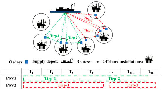
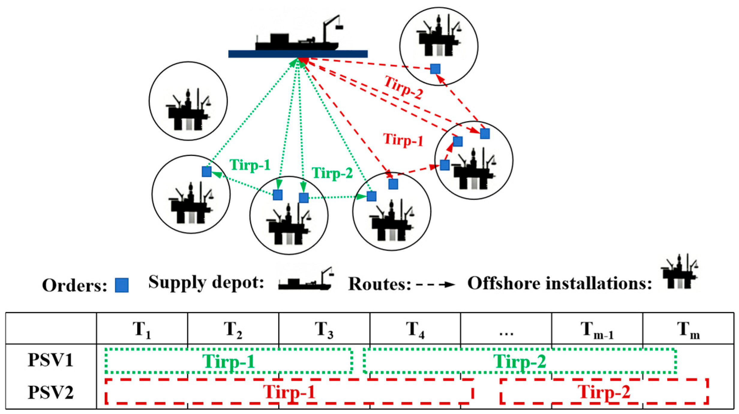
In practical offshore logistics operations, the PSVRSP can be described on a graph , where the node set represents order locations, and the arc set represents sailing legs, each associated with the sailing distance between pairs of orders. Let denote the set of offshore platforms that require service, and the set of all orders to be performed. Let be the unit cargo-handling rate at each offshore platform, and the set of available PSVs. In this work, a trip is defined as a complete voyage cycle performed by a single vessel, consisting of three sequential tasks: (i) departing empty from the onshore supply base; (ii) serving orders offshore; and (iii) returning to the onshore supply base to unload any pickup cargo collected during the trip. Each vessel is allowed to complete at most consecutive trips. The entire sequence of trips performed by a vessel is collectively referred to as a route. Figure 1 illustrates the structure of the transportation network, including the spatial distribution of offshore installations and the time-indexed table at the bottom, which explicitly shows the time occupied by each trip and ensures that no vessel is assigned overlapping tasks.
Figure 1.
Illustrative diagram of a PSVRSP.
In addition, several practical and commonly adopted modeling assumptions are introduced to ensure the rationality and operability of the proposed optimization framework. First, all platform supply vessels (PSVs) are assumed to be homogeneous in terms of sailing speed, cargo capacity, and unit operational cost. Second, the planning horizon is predefined and fixed, and no emergent or temporary tasks arise during the scheduling cycle. Third, vessel sailing speed is assumed to be constant, and sailing time is determined solely by travel distance, while short-term meteorological disturbances are neglected. Fourth, each offshore demand order must be served entirely by a single vessel; therefore, split deliveries and partial services are not allowed. Fifth, vessels are permitted to visit duplicated supply-base nodes only in a strict sequential order, which standardizes multi-trip scheduling and prevents cross-trip route conflicts. In addition, the assumption of demand independence across different offshore installations is explicitly stated and discussed in the Numerical Experiments section to characterize stochastic demand uncertainty.
To clarify the fundamental scheduling unit and facilitate subsequent model construction and algorithm design, the formal definition of a trip is provided below.
Definition 1.
A trip is composed of an ordered node sequence , a planned start time , a maximum postponable time and a planned end time such that:
- The total loading demand on the sequence does not exceed the vessel’s capacity constraint;
- The vessel can start service at , serve all orders according to the given sequence, return to the onshore supply base, and satisfy all time windows and sailing time constraints;
- The planned start time and maximum postponable time jointly form the feasible departure time interval of the trip, covering all valid departure times under the visiting sequence.
Mathematical Modeling
In this section, we present an MILP formulation for the PSVRSP-UD. Before we proceed, we first introduce some pertinent notation. Table 1 lists the sets, parameters, and variables involved in the model.
Table 1.
Notation of sets, parameters and variables.
In this study, duplicated supply base nodes are used to model the multi-trip scheduling problem for a single vessel [24]. By constructing an ordered chain of depot-copy nodes to characterize the trip sequence, cross-trip service is avoided without introducing additional trip-index variables. To ensure the sequential use of duplicated supply base nodes, the arc set A is defined as , where represents the arc set between customer nodes, represents the arc set from duplicated supply base nodes to customer nodes, represents the arc set from customer nodes to duplicated supply base nodes, and represents the sequential arc set between consecutive duplicated supply base nodes. This definition ensures that supply vessels can only visit duplicated supply base nodes in strict trip sequence within the planning horizon, and any non-sequential jump across trips is prohibited.
The PSVRSP-UD model aims to generate feasible routes and schedules for platform supply vessels (PSVs) to minimize the total cost while satisfying all order fulfillment and operational constraints. As PSVs represent one of the costliest resources in offshore logistics, and in response to the requirements of energy conservation and emission reduction in international shipping, the total cost consists of vessel operating cost and carbon emission cost, where is a weight coefficient that balances the importance of the two cost components. A larger emphasizes operational efficiency, while a smaller α indicates greater focus on carbon emission reduction. In practical applications, can be chosen to reflect corporate operational strategies and low-carbon policies. The carbon emission cost adopts the fuel consumption function proposed by Psaraftis and Kontovas [25], which comprehensively considers the nonlinear relationship among demand scenario probability, vessel speed, payload, and fuel consumption. The complete MIP model of PSVRSP-UD is as follows.
Subject to
The objective function (1) is to minimize the expected value of the total cost over all demand scenarios. Constraint (2) is the out-degree constraint for the starting duplicated supply base node. Constraint (3) is the in-degree constraint for the ending duplicated supply base node. Constraint (4) is the flow conservation constraint for intermediate duplicated supply base nodes, ensuring the orderly connection between consecutive trips. Constraint (5) is the flow balance constraint for order nodes. Constraint (6) is the uniqueness constraint, ensuring each order is served exactly once. Constraint (7) ensures that each vessel must visit the duplicated supply base nodes in sequence. Constraint (8) is the maximum payload constraint, ensuring the vessel load does not exceed capacity Q under any demand scenario. Constraint (9) is the payload update constraint, ensuring the load of vessel under scenario s is properly updated when traversing arc . Constraint (10) is the payload reset constraint, ensuring the vessel completes unloading at each intermediate duplicated supply base node. Constraint (11) defines the calculation of vessel sailing time. Constraint (12) defines the calculation of order service time. Constraints (13)–(14) are order service time window constraints, ensuring the service start time falls within the specified interval. Constraint (15) is the time continuity constraint, ensuring the start time of service for order j is no earlier than the completion time of service for order plus the sailing time from to . Constraints (16)–(18) are variable definition constraints.
4. Proposed Branch-And-Price Algorithm for the PSVRSP-UD
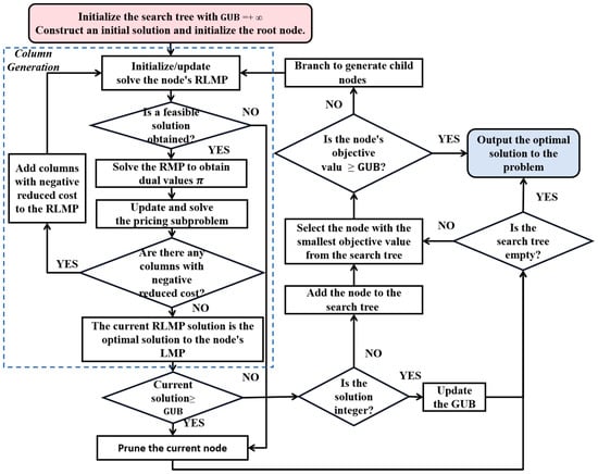
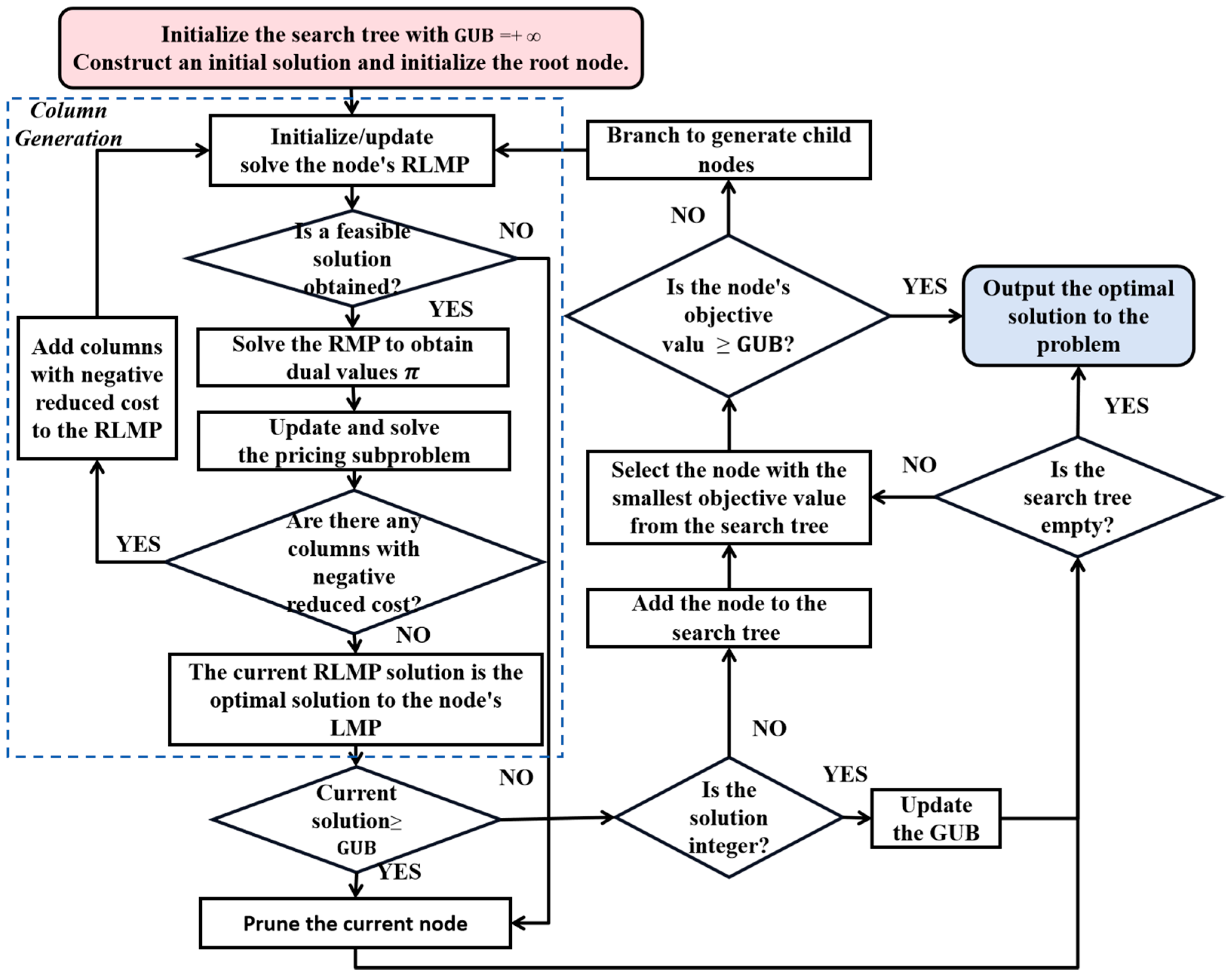
To precisely solve the PSVRSP-UD, this study designs and implements a B&P algorithm [26]. Its core idea is to embed column generation (CG) within a branch-and-bound (B&B) framework [27]. By dynamically generating feasible trips with negative reduced cost, it avoids the combinatorial explosion caused by explicitly enumerating all routes, thereby achieving efficient global optimal solution of large-scale integer programming models. From a theoretical perspective, the proposed framework follows the standard branch-and-price paradigm, in which column generation is embedded within a branch-and-bound procedure. It is well established in the literature that, for branch-and-price, convergence to the global optimum is guaranteed when the pricing subproblem is solved to optimality and the branching scheme ensures a complete partition of the feasible solution space [27]. In this study, both conditions are satisfied, which guarantees the optimality of the final solution.
To enhance the clarity of the algorithmic framework, a flow chart of the proposed branch-and-price procedure is provided in Figure 2, which illustrates the interaction between the master problem, pricing subproblem, and branching process.
Figure 2.
Flow chart of the B&P algorithm.
The following sequentially presents the model reformulation, pricing subproblem solution, branching strategy, and integer solution repair mechanism.
4.1. Model Reformulation via Dantzig–Wolfe Decomposition
The PSVRSP-UD is essentially analogous to the multi-trip vehicle routing problem with time windows (MTVRPTW). For such multi-trip routing and scheduling problems, two typical set-partitioning models have been widely studied. The first model uses a complete vessel route as a column, directly representing a consecutive multi-trip sequence from departure to return [28]. Although structurally intuitive, this leads to an explosion of the column space due to the combination of trip connections and time schedules, making it impractical for real-scale instances. The second model takes a single trip as the basic column unit and does not explicitly model the full route of a vessel [29]. This model controls the non-overlapping trips of the same vessel via constraints, drastically reducing problem complexity and difficulty. This study adopts the second modeling approach and follows the exact solution paradigm for multi-trip problems.
The cost of trip under scenario is denoted , and the set of trips is denoted . Based on this definition, the PSVRSP-UD can be modeled as a set-partitioning problem with mutual exclusion constraints, where denotes whether trip is selected, and the set to be covered is the order demand of offshore platforms. Mutual exclusion constraints ensure that selected trips can be assigned to K PSVs without overlapping in time for the same PSV. This paper ensures that most K PSVs are used at any time. By discretizing time, a Boolean indicator is defined to indicate whether trip covers time , such that the number of occupied vessels at any time does not exceed the fleet size.
The resulting set-partitioning formulation of the PSVRSP-UD is presented as follows:
Subject to
where indicates whether order is covered by trip and is the number of decimal digits for time precision. This objective (19) minimizes the expected total cost over all scenarios and selected trips. Constraint (20) ensures each order is served once. Constraint (21) ensures the number of PSVs used at any time interval does not exceed the fleet size limit.
To avoid an explosion of constraints due to overly fine time precision, this study adopts a coarse time interval relaxation strategy. If the relaxed solution is feasible, it is optimal; otherwise, the granularity is refined. Specifically, the planning horizon is partitioned as follows. Let be a small value guaranteeing that the duration of any feasible trip is greater than . The interval is partitioned as , and constraint (21) is replaced by constraint (23).
where is the time proportion of trip within interval . As is smaller than any trip duration, can accurately compute the start time of any trip without loss of precision. If the optimal relaxed solution is infeasible (violating (21)), then is halved and recomputed.
The relaxed linear master problem (RLMP) is formulated as follows:
Subject to
where is the restricted set of columns (trips) generated dynamically in column generation.
4.2. Pricing Subproblem: NG-Route Labeling Algorithm
The pricing subproblem seeks a trip with negative reduced cost under all scenarios. Given dual values and corresponding to constraints (25) and (26) of the RLMP, the reduced cost for is presented as follows.
This subproblem can be viewed as the elementary shortest path problem with resource constraints (ESPPRC) [30], typically solved by a dynamic programming labeling algorithm. The ESPPRC is known to be NP-hard due to the presence of resource constraints such as time windows and capacity limitations. In the context of PSVRSP-UD, the problem becomes even more challenging as resource feasibility must be maintained simultaneously across multiple demand scenarios, which significantly increases the dimensionality of the state space. However, for the PSVRSP-UD studied in this paper, the traditional labeling algorithm faces two challenges:
- The search space of the pricing subproblem corresponds to trips, and the time dual variable leads to different reduced costs for different departure times of the same order sequence;
- Multi-scenario demand constraints require each label to track resource consumption and feasibility under all demand scenarios, significantly increasing label dimension and pruning difficulty.
To improve computational efficiency and avoid this combinatorial difficulty, this paper introduces the NG-route relaxation strategy [29] into the labeling algorithm, combined with the group of labels and representative label mechanisms [31]. The theoretical validity of this mechanism follows the proven framework in Hernández et al. (2016) [32]. Labels in the same group correspond to identical paths and differ only in departure times; thus, retaining a single representative label with the earliest arrival time is sufficient to recover all feasible schedules in the group without loss of optimality. The designed dominance rule is formally guaranteed to prune only dominated labels and will never discard potentially optimal paths. This group-label mechanism avoids redundant enumeration of identical visiting sequences with different departure times. Instead of generating multiple labels for each feasible departure time, a single representative label captures the entire feasible departure interval, which significantly reduces the number of labels and improves computational efficiency while preserving global optimality.
4.2.1. Definition of NG-Labels
The ESPPRC is defined on a directed graph , where nodes and represent the onshore supply base as the path start and end, respectively. Under the NG-route relaxation framework, a neighborhood set is predefined for each node , consisting of the closest nodes to . Path extension is only allowed within the neighborhood, thereby significantly compressing the state space. Meanwhile, to avoid generating numerous duplicate labels with the same path but different times due to different departure times, this paper further introduces the group of labels and representative label mechanism. The core logic includes the following:
- All labels in the same group correspond to an identical visiting sequence path, differing only in departure time;
- Only one representative label is retained per group, and the postponable time rt(∙) describes the flexible range of all feasible departure times within the group, such that every feasible trip in the same group can be derived from the representative label.
On this basis, an NG-label characterizes the partial path state of the vessel under multi-scenario demand, time windows, and capacity constraints. Compared with traditional labels, the NG-label not only records path information but also contains a neighborhood set to control the extension direction, further improving efficiency.
Each label stores the following data, and describe the visited sequence and current node; is the parent label; records the vessel load under all demand scenarios; , and characterize the temporal state and flexibility of the trip, respectively; and represents the accumulated reduced cost, and is the neighborhood set of the current node .
4.2.2. Label Extension Rules
The label extension procedure consists of two steps: feasibility checking and label updating, as described below. In the extension phase, each label extension is checked for feasibility according to the following constraints.
Neighborhood constraint: Only extend to nodes in the neighborhood of the current node .
Time window constraint: Ensure the vessel’s arrival time does not exceed the latest service time of the node.
Load constraint: Vessel load must not exceed the maximum capacity under all scenarios.
where is the current load in scenario s.
If all constraints are satisfied, a new label is generated with updated information.
Equations (32)–(40) update the information of the newly generated label , including the path extended to the new node , the current node position, the parent label, the vessel’s load upon across all scenarios, the departure time from , the trip start time, the updated arrival and departure time at the new node, the maximum feasible postponement time, and the updated neighborhood set. In Equation (39), denotes the index of the discretized time interval that contains the time . Let and represent the lower and upper bounds of the time interval , respectively. A small positive constant is introduced in order to avoid a division by 0 when . With this definition, the dual variables are accumulated proportionally according to the proportion of time interval included in [, ]. Overall, these update rules ensure that each extended label remains feasible with respect to time windows and capacity constraints under all demand scenarios.
4.2.3. Dominance Rule
In the labeling algorithm, the design of the dominance rule determines computational efficiency. The core idea is that, if one label at the same node is not better than another in terms of resource consumption and cost, it cannot lead to a better solution and can be pruned early. Traditional dominance strategies are usually based on the deterministic shortest path framework. However, given the multi-scenario demand and temporal flexibility of labels in the PSVRSP-UD, the following dominance criterion is designed. A label dominates another label if all following conditions are satisfied simultaneously.
Conditions (41)–(46) ensure that label 1 is strictly better in path, load, time, flexibility, and cost. Intuitively, this rule ensures that a label is discarded if another label exists that is no worse in all resource dimensions and strictly better in at least one dimension. This dominance rule reduces the number of labels and improves the efficiency of the pricing subproblem without losing optimality. From a theoretical perspective, the dominance rule ensures that inferior labels are pruned without excluding any potentially optimal solution. This property is essential for maintaining both correctness and computational tractability of the labeling algorithm.
To further clarify the overall procedure, the labeling algorithm is summarized in Algorithm 1.
| Algorithm 1: NG-Route Labeling Algorithm for the pricing subproblem | |
| Input: Graph G, neighborhood sets, demand scenarios, dual variables, vessel information, order information | |
| Output: Set of feasible trips with negative reduced cost | |
| 1 | Initialize label at depot |
| 2 | Add initial label to list |
| 3 | While label list is not empty do |
| 4 | |
| 5 | For do |
| 6 | Check time feasibility |
| 7 | Check capacity feasibility (all scenarios) |
| 8 | If feasible then |
| 9 | |
| 10 | Update time, load, and cost |
| 11 | Apply dominance rule |
| 12 | If not dominated then |
| 13 | to label list |
| 14 | End if |
| 15 | End if |
| 16 | End for |
| 17 | If can return to depot with negative reduced cost then |
| 18 | Generate a new column |
| 19 | End if |
| 20 | End while |
4.3. Branching Strategy and Integer Solution Repair
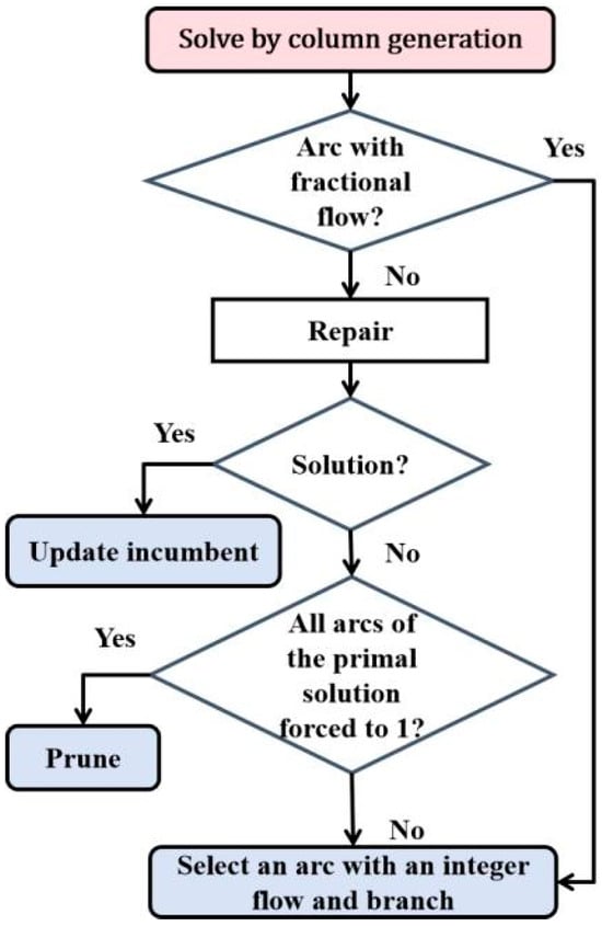
Solving the RLMP via CG only obtains a linear relaxation solution. To obtain an optimal schedule satisfying integer constraints, CG must be embedded within a B&B framework to form a complete B&P algorithm. However, in multi-trip scheduling problems such as the PSVRSP-UD, the traditional arc branching strategy has obvious limitations. This limitation arises because in multi-trip scheduling problems, integer arc flows do not necessarily imply integer trip selections. The same sequence of visited nodes may correspond to multiple feasible trips with different departure times, leading to fractional solutions even when arc variables are integral. Therefore, additional mechanisms are required to enforce integrality at the trip level. Even if all arc flows are integer-valued, trip variables may still be fractional. This occurs because the same visiting sequence can form multiple feasible trips at different departure times, making arc flows unable to uniquely determine the time schedule of trips. To address this issue, this section designs a two-level branching strategy tailored to the problem’s characteristics, as shown in Figure 3.
Figure 3.
Proposed two-level branching strategy.
If a fractional-flow arc exists, the conventional arc branching strategy is applied. If all arc flows are integer, a repair procedure is initiated to construct an integer trip schedule without time conflicts. All feasible trip structures in the current fractional solution are treated as virtual customers, constructing an auxiliary VRPTW subproblem. Each virtual customer corresponds to a trip node sequence , with time window [,] representing the feasible start interval of the sequence; service time and demand are set to 0; the fleet size is consistent with the original problem. The goal is to assign a conflict-free service sequence to these virtual customers, i.e., to construct a set of integer trips without overlapping times. The auxiliary VRPTW problem is solved by CG. If a feasible integer solution is obtained, the global optimal upper bound is updated and the current node is pruned. If repair fails, no integer solution can be formed based on the structures in the current solution, implying at least one arc in these structures does not belong to the optimal solution. A standard branching rule is applied on unconstrained arcs, creating two branches that force the arc flow to 0 and 1, respectively. If no feasible solution exists after all arcs with flow 1 are forbidden, the current node is directly pruned.
This two-level branching strategy effectively resolves the special issue of integer arc flows but fractional trip variables in multi-trip scheduling, guaranteeing that the algorithm converges to the global optimal solution. The proposed two-level branching strategy explicitly addresses this structural issue. The first level eliminates fractional arc flows, while the second level resolves temporal ambiguity among trips by enforcing non-overlapping schedules. This combination ensures that the branching process remains complete and leads to a valid integer solution. Therefore, the overall branch-and-price algorithm is guaranteed to produce an optimal integer solution.
5. Numerical Experiments
To verify the effectiveness of the proposed model and algorithm, various computational experiments are conducted. The flow-based MILP model was solved using ILOG CPLEX 12.9, implemented in C++, with a time limit of 3600 s. All experiments were conducted on a Windows 10 system with an Intel(R) Core(TM) i5-8500 CPU @ 3.0 GHz and 8 GB RAM.
5.1. Test Instances and Parameter Settings
5.1.1. Demand Uncertainty Modeling and Scenario Generation
In this section, we present a method to approximate the probability distribution of demand at offshore installations. We assume that demands at different installations are mutually independent; that is, demand at each installation follows an independent probability distribution, which may include normal, Erlang, or Weibull distributions [9]. Based on such probabilistic representations, several modeling approaches can be employed, including robust optimization, chance-constrained programming, and scenario-based stochastic programming. Robust and chance-constrained models provide protection against uncertainty but may lead to overly conservative decisions or complex probabilistic constraints [33]. By comparison, scenario-based stochastic programming discretizes the underlying demand distribution into a finite set of representative realizations, which supports direct comparisons across different demand outcomes. Given this balance between modeling fidelity and computational tractability, this study adopts scenario-based representations. To incorporate this uncertainty into the model, demand is treated as a random variable, and a combination of scenario generation and scenario reduction approach is employed.
To generate a diverse set of demand scenarios, this study adopts an approach that combines LHS and Cholesky decomposition [34]. LHS provides stratified sampling that ensures more uniform coverage of multidimensional distribution space. However, when sampling multiple random variables, their inherent correlation may reduce the representativeness of the generated scenarios. To address this issue, Cholesky decomposition is incorporated to weaken inter-order demand correlations, thereby improving independence and diversity of the scenario set.
Suppose there are orders, and their demands are represented by . The cumulative distribution function for the demand at order is expressed as follows,
Using this formulation, a total of M scenarios is generated through the process. First, an ordered sampling matrix is constructed via the LHS method. Next, the Cholesky decomposition is applied to adjust the sampled vectors and mitigate correlation among port demands. The final output is an M-scenario demand matrix for the orders, completing the multi-scenario generation procedure.
To improve computational efficiency and reduce redundant scenarios, the stepwise backward reduction (SBR) algorithm [35] is applied. This algorithm iteratively computes the distances between scenarios and removes the scenario with the smallest distance to others until the initial scenarios are reduced to the predefined number. The final output consists of representative scenarios and their associated probabilities. Specifically, denotes the scenario set , and each scenario occurs with probability .
5.1.2. Instance Configuration
This section specifies the test instances and parameter settings adopted for PSVRSPUD. The benchmark instances are constructed based on real-world operational data from an oil and gas company operating in Brazilian waters, as reported in Silva’s work [36]. A total of six offshore platforms are selected to form the test network. The sailing time from the onshore supply base to each platform ranges from 16 to 19 h, and the average sailing time between any two platforms is 1.1 h. During the planning horizon, each platform generates a random number of service orders. For each order, the expected demand is uniformly distributed in the interval [70, 150]. To capture demand uncertainty, a scenario generation and reduction method is employed to construct a set of representative demand scenarios denoted by . Each scenario is assigned with an occurrence probability . The actual demand under each scenario follows a normal distribution with the expected demand as the mean and a standard deviation . Each standard deviation corresponds to a distinct demand variation level, which enables a comprehensive evaluation of the impact of different demand uncertainty degrees on scheduling decisions. For time-related parameters, the service time windows are generated in accordance with the classic Solomon scheme. The earliest arrival time at each node is determined by the sailing distance, and the width of each time window ranges from 30 to 70 h, which does not exceed the total planning horizon of 168 h.
Each instance is named according to a consistent rule that includes the number of platforms, orders, vessels, and the standard deviation of demand. For illustration, the instance name c6-o12-v3-d3-5 indicates an instance with 6 platforms (c), 12 orders (o), 3 vessels (v), a demand standard deviation of 0.3 (d), and the replicate index (n) 5.
5.2. Experimental Results and Analysis
5.2.1. Performance of the B&P Algorithm
The performance of the proposed B&P algorithm is compared with the flow-based model solved by CPLEX 12.9. Experiments in this section are conducted under a fixed demand standard deviation () and a weight coefficient (), considering 10 demand scenarios. In each instance, statistical comparisons are performed on multiple metrics, including objective function value (Obj), computational time (T), upper bound (UB), lower bound (LB), gap (), and relative deviation ().
The comparative results of the algorithms on different test instances are summarized in Table 2 and Table 3. For small-scale instances with 4–8 orders, both CPLEX and B&P can obtain optimal solutions within the 3600 s time limit. In terms of computational efficiency, the B&P algorithm exhibited a significant advantage. The objective values are exactly the same, and the relative deviation (RD) is 0%, which verifies that the optimal solutions obtained by the B&P algorithm are consistent with those of CPLEX. In terms of computational efficiency, the B&P algorithm demonstrates a remarkable advantage. For instances with four orders, the average solution time of B&P is only 0.012 s, while CPLEX requires approximately 0.25 s, making B&P more than 95% faster on average. For instances with 8 orders, the computational time of CPLEX increases sharply to a range of 522.5 s to 1586.91 s, with an average of 461.97 s. In contrast, the B&P algorithm solves the same instances in only 0.02 s to 1.7 s, with an average of merely 0.31 s. These results also indicate that B&P’s advantage in computational efficiency becomes more pronounced with modest increases in problem size.
Table 2.
Comparison of B&P and CPLEX results for small-scale instances.
Table 3.
Comparison of B&P and CPLEX results for medium- and large-scale instances.
For medium- and large-scale instances (involving 12 to 28 orders), CPLEX 12.9 fails to obtain optimal solutions within the 3600 s time limit. As reported in Table 3, the average optimality gap of CPLEX reaches 97.24%, and the gap generally increases with the problem size, indicating a rapid deterioration in the quality of the linear relaxation for large-scale PSVRSP-UD instances. For several large instances, CPLEX is unable to sufficiently tighten the lower bound within the time limit, leading to weak dual bounds and limited solution quality. In addition, for some instances, either the lower bound or both bounds are not further improved within the time limit, resulting in missing entries (“–”) in Table 3 due to premature termination before meaningful bound updates can be obtained. These results demonstrate that the flow-based formulation is not scalable for solving large-scale instances of the considered problem.
In contrast, the proposed branch-and-price (B&P) algorithm shows significantly stronger performance in both solution quality and computational efficiency. For medium-scale instances (12–24 orders), the B&P algorithm consistently obtains optimal solutions with zero optimality gap. The solutions either match or improve the upper bounds reported by CPLEX, while requiring substantially less computational time. The average runtime of the B&P algorithm is 1103.66 s, compared with the full 3600 s time limit required by CPLEX, demonstrating its superior efficiency.
For large-scale instances (28 orders), the B&P algorithm is further tested on a selected set of representative and computationally challenging instances. As the problem size increases, the underlying structure becomes significantly more complex, leading to an exponential growth in the number of feasible routes and pricing subproblems. This results in a combinatorial explosion in the labeling process, making the column generation procedure increasingly difficult to converge within the given time limit. In addition, demand uncertainty further increases the computational burden by introducing multiple demand realizations, which expand the effective decision space and strengthen the coupling between routing decisions and stochastic outcomes. As a result, although the B&P algorithm still obtains optimal solutions for several instances, a few cases exhibit mild optimality gaps ranging from 1.28% to 11.32% due to time limit termination. This behavior is consistent with the characteristics of exact branch-and-price methods for large-scale stochastic combinatorial optimization problems. Despite this, the solution quality remains strong, and all solutions are within or improving upon the upper bounds reported by CPLEX. The RD analysis further confirms the advantage of the proposed method, with an average RD of −4.48%, indicating that the B&P algorithm generally produces better solutions than CPLEX. In particular, instance c6-o20-v3-d3-4 achieves the largest improvement, with an RD of −12.74%, while several instances show identical performance between the two methods (RD = 0.00%).
In summary, the B&P algorithm significantly outperforms CPLEX in both solution quality and computational efficiency. It can obtain exact solutions within a reasonable computational time and exhibits robust convergence behavior, making it highly suitable for complex real-world PSVRSP applications. As this study focuses on exact optimization methods, the comparison is primarily conducted against CPLEX; incorporating heuristic approaches as additional benchmarks is left for future research due to the focus on exact solution quality in this study.
5.2.2. Sensitivity Analysis on Number of Scenarios
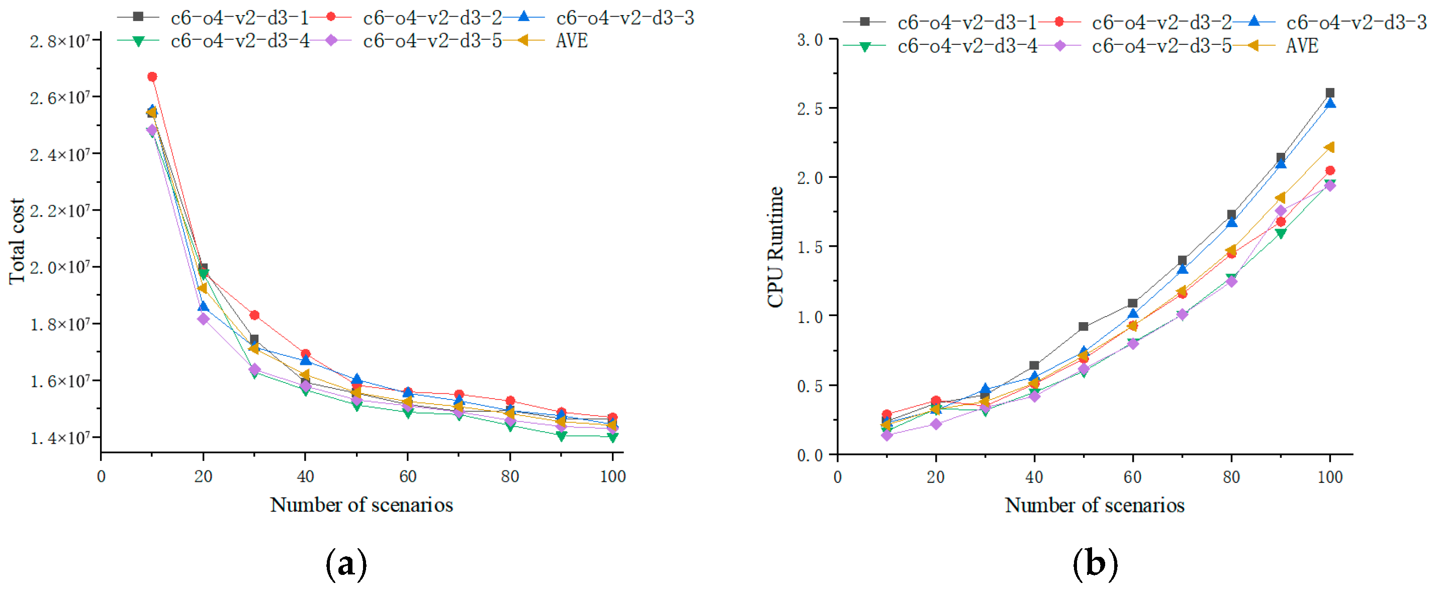
To investigate the influence of the number of demand scenarios on solutions under demand uncertainty, this section conducts a sensitivity analysis on the 4-port instance c6-o4-v2-d3-n, varying the number of scenarios from 10 to 100. The total cost and CPU time are illustrated in Figure 4. It shows that the total cost exhibits a significant downward trend as the number of scenarios increases from 10 to 100, rather than remaining robust as previously described. Specifically, the average total cost of the five instances decreases from 25,456,139.56 (10 scenarios) to 14,426,007.87 (100 scenarios), with a total reduction of approximately 43.33%. This indicates that increasing the number of scenarios can better capture the characteristics of demand uncertainty, and that the optimal scheduling decisions are gradually adjusted to be more cost-effective as the scenario number increases.
Figure 4.
Sensitivity analysis for the number of scenarios: (a) Total cost and (b) computational time.
In terms of computational efficiency, the algorithm’s runtime shows a stable positive correlation with the number of scenarios. For example, the CPU runtime of c6-o4-v2-d3-1 increases from 0.24 s to 2.61 s; for c6-o4-v2-d3-5, the runtime rises from 0.14 s to 1.94 s. On average, the runtime of the five instances increases from 0.214 s to 2.218 s, which is a tenfold increase but still remains at a low level, ensuring high computational efficiency.
To mitigate the increased computational burden, a scenario reduction technique is employed in this study. The scenario reduction method aims to preserve the most representative demand realizations while reducing computational complexity. Although some approximation is introduced, the sensitivity analysis shows that increasing the number of scenarios leads to more stable and cost-effective solutions, indicating that the reduction process keeps the essential characteristics of demand uncertainty.
Overall, the results indicate that the scenario setting adopted in this study can balance the trade-off between solution quality and computational efficiency.
5.2.3. Sensitivity Analysis on Demand Fluctuation Levels
To investigate the impacts of demand uncertainty on scheduling results, this section conducts a sensitivity analysis under different levels of demand fluctuation. Tests are carried out on the 8-order instance c6-o8-v2-n as an example; the standard deviation of demand is varied. Specifically, σ is set to 0.1, 0.2, 0.3, 0.4, and 0.5, representing increasing uncertainty levels. All other parameters remain unchanged. The detailed results are reported in Table 4.
Table 4.
Sensitivity analysis for demand variability.
In terms of solution quality, the total cost generally shows an upward trend as demand uncertainty increases. As σ rises from 0.1 to 0.5, the average total cost increases from 52,513,500.63 to 52,998,710.12, indicating that higher demand volatility requires more conservative scheduling and additional capacity reserves to ensure feasibility, thereby raising the overall operational cost. At the instance level, most test problems show a gradual rise in objective value with increasing σ, reflecting the additional economic burden induced by demand uncertainty. Regarding computational efficiency, an overall decline in solution time can be observed as σ increases. The average computing time decreases monotonically from 1256.17 s at σ = 0.1 to 800.82 s at σ = 0.5. This phenomenon suggests that stronger demand uncertainty leads to a more constrained solution space and tighter feasibility conditions, which in turn accelerates the convergence of the algorithm and reduces the overall solution time without significantly compromising solution quality.
In summary, increasing demand fluctuation results in higher total expected cost due to the need for more robust scheduling arrangements, while simultaneously improving the computational efficiency of the proposed B&P algorithm.
5.2.4. Sensitivity Analysis on Time Window Tightness
To examine the impact of temporal constraints on optimal scheduling decisions, a sensitivity analysis is conducted with respect to time-window tightness. The experiments are performed on the 4-order test instances c6-o4-v2-d3-n, while all other model parameters are held constant. Three representative levels of time-window tightness are considered: tight (tw0), moderate (tw1), and loose (tw2). These time-window settings are generated following the Solomon-style scheme by varying the width of service time windows.
The resulting optimal scheduling outcomes under different time-window configurations are evaluated in terms of total sailing time (ST) and total sailing distance (SD). The corresponding results are summarized in Table 5, which illustrates how varying degrees of temporal flexibility affect the structure and efficiency of the optimal schedules.
Table 5.
Sensitivity analysis for time window tightness.
The experimental results indicate that time-window tightness has a clear and consistent influence on sailing time, sailing distance, and, consequently, total operational cost. As time windows become looser, the overall solution quality improves steadily.
With respect to sailing time (time in best cost), the average value exhibits a mild decreasing trend as time-window flexibility increases. Specifically, the average sailing time decreases from 129.81 under tight time windows (tw0) to 127.89 under medium time windows (tw1), and then slightly increases to 128.22 under loose time windows (tw2). This pattern suggests that relaxing time windows provides additional scheduling flexibility, enabling vessels to better coordinate service sequences and reduce unnecessary waiting or detours. However, the overall variation in sailing time remains modest, indicating that time-related adjustments are not the primary driver of cost reduction.
In contrast, sailing distance (distance in best cost) shows a more pronounced and monotonic decrease as time windows are relaxed. The average sailing distance is reduced from 1531.61 (tw0) to 1513.22 (tw1) and further to 1494.94 (tw2), corresponding to an overall reduction of approximately 2.39%. This finding indicates that looser time windows allow the model to construct more compact and efficient routing structures by eliminating inefficient paths and improving route consolidation.
These effects are further reflected in the total cost performance. The average total cost decreases from 12,475,712.64 under tight time windows to 12,318,132.03 under medium time windows, and further to 12,169,749.70 under loose time windows. This confirms that tighter time-window constraints impose stricter feasibility requirements, which limit routing flexibility and lead to higher operational costs.
Overall, although time-window tightness significantly affects scheduling flexibility, its impact on sailing time is relatively limited, whereas its influence on sailing distance and total cost is more substantial. This suggests that the primary benefit of relaxing time-window constraints lies in improved route optimization rather than temporal adjustments alone.
In summary, the results demonstrate that the proposed model is sensitive to temporal constraints while remaining stable across different time-window settings. From a practical perspective, moderately relaxed time windows can effectively reduce operational costs and enhance routing efficiency, whereas excessively tight constraints may result in inefficient and costly scheduling solutions.
5.2.5. Sensitivity Analysis on Weight Coefficient
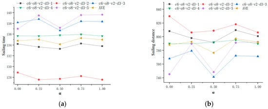
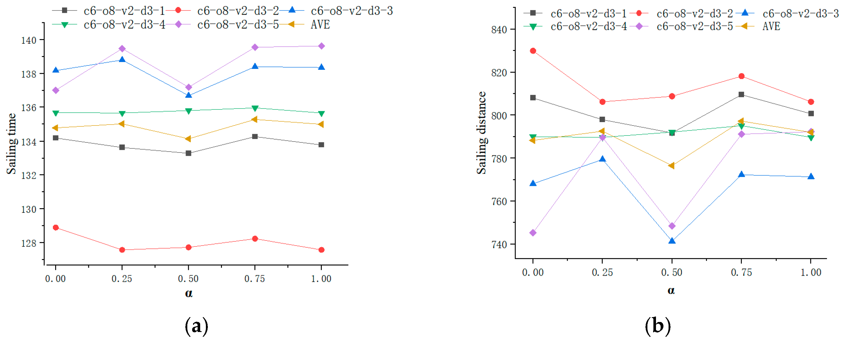
To explore the impact of economic objectives and low-carbon objectives on the optimal scheduling scheme, a sensitivity analysis is conducted with respect to the weight coefficient . Tests are carried out on 8-order instance c6-o8-v2-d3-n as an example; all other parameters are held constant. Specifically, is set to five typical levels: 0, 0.25, 0.5, 0.75, and 1, where a larger indicates greater emphasis on minimizing operational time cost, and a smaller highlights the control of carbon emissions. The corresponding results of sailing time and sailing distance of the optimal scheduling scheme under different weight configurations are presented in Figure 5.
Figure 5.
Sensitivity analysis for the weight coefficient: (a) Sailing time of the optimal scheduling scheme and(b) sailing distance of the optimal scheduling scheme.
Experimental results show that the weight coefficient has a mild but stable impact on both sailing time and distance, without causing significant fluctuations or monotonic trends. When varies from 0 to 1, the sailing time (time in best cost) maintains a relatively steady level across all 8-order instances. Specifically, the sailing time ranges approximately between 127.59 and 138.40, with no abrupt increases or decreases. For example, the time for instance c6-o8-v2-d3-2 remains 127.59 when = 0.25 and = 1, while the time for c6-o8-v2-d3-3 reaches the maximum of 138.80 when 0.25, showing only slight variations across different levels.
In terms of sailing distance (distance in best cost), it also remains stable with the change of . The distance ranges between 741.38 and 829.96, with no obvious monotonic trend as increases or decreases. For most instances, the distance fluctuates slightly within a narrow range across different levels; for example, the distance of c6-o8-v2-d3-4 varies only between 789.71 and 795.14, with a maximum variation of less than 0.7%.
Although adjusts the trade-off priority between operational time cost and carbon emission cost, the optimal scheduling scheme remains robust and efficient. The stable sailing time and distance across different levels indicate that adjusting the weight coefficient does not alter the core structure of the optimal route. In practical applications, decision-makers can flexibly select an appropriate according to corporate emission-reduction policies, operational budgets, or energy-saving requirements, without causing obvious deterioration in sailing efficiency or route rationality.
6. Conclusions
This study addresses the platform supply vessel routing and scheduling problem under demand uncertainty, aiming to minimize the expected total cost, including vessel operating and carbon emission costs, while satisfying key operational constraints such as capacity, time windows, and multi-trip requirements. A scenario-based MILP model is developed to capture stochastic offshore demand, where uncertainty is represented through a finite set of scenarios generated using LHS combined with Cholesky decomposition. Scenario reduction is further applied to improve computational efficiency while preserving solution quality. To solve the resulting NP-hard problem, a branch-and-price algorithm is proposed, integrating Dantzig–Wolfe decomposition and an enhanced labeling scheme with a tailored branching strategy. Computational results show that the proposed B&P algorithm consistently outperforms CPLEX 12.9 in terms of both solution quality and efficiency. It achieves optimal solutions for all tested instances, while CPLEX fails to converge within the time limit for medium- and large-scale cases. Sensitivity analyses indicate that scenario settings effectively balance solution quality and computational effort, and that higher demand uncertainty increases total cost while having limited impact on computational stability. The weighting parameter between operational and emission costs provides flexible trade-offs for decision-making. Future work may extend this study by incorporating correlated demand structures, multi-source uncertainties such as weather conditions, and more advanced solution acceleration techniques, including parallel computing, improved pruning strategies, and comparisons with state-of-the-art heuristic algorithms.
Author Contributions
Conceptualization, B.J. and J.L.; methodology, B.J. and J.L.; software, J.L.; validation, B.J., J.L. and S.S.Y.; formal analysis, J.L.; investigation, J.L.; resources, B.J.; data curation, J.L.; writing—original draft preparation, B.J. and J.L.; writing—review and editing, B.J. and S.S.Y.; visualization, J.L.; supervision, B.J. and S.S.Y.; project administration, B.J.; funding acquisition, B.J. All authors have read and agreed to the published version of the manuscript.
Funding
This research was funded by National Natural Science Foundation of China, grant number No. 72371250; Natural Science Outstanding Youth Foundation of Hunan Province, China, grant number No. 2024JJ4073 and The Science and Technology Innovation Program of Hunan Province, China, grant number No. 2024RC3011.
Data Availability Statement
The original contributions presented in this study are included in the article. Further inquiries can be directed to the corresponding author.
Conflicts of Interest
The authors declare no conflicts of interest.
References
- Guo, L.; Song, W.; Long, Y. Maritime service network design with oil-fueled and LNG-fueled mixed vessel fleet under uncertainty: Overview and future research directions. Transp. Econ. Manag. 2025, 3, 423–431. [Google Scholar] [CrossRef] [Scilit]
- Shu, Y.; Guo, Y.; Du, Y.; Wang, S. A Mixed-Integer Linear Programming Framework for Multi-Period Offshore Wind Personnel Logistics: Integrating Routing, Scheduling, and Personnel Inventory Management. Mathematics 2026, 14, 978. [Google Scholar] [CrossRef] [Scilit]
- Friedberg, D.O.; Uglane, V.T. Routing and Scheduling of Platform Supply Vessels; Norwegian University of Science and Technology: Trondheim, Norway, 2013. [Google Scholar]
- Fagerholt, K.; Lindstad, H. Optimal policies for maintaining a supply service in the Norwegian Sea. Omega 2000, 28, 269–275. [Google Scholar] [CrossRef] [Scilit]
- Aas, B.; Gribkovskaia, I.; Halskau, Ø., Sr.; Shlopak, A. Routing of supply vessels to petroleum installations. Int. J. Phys. Distrib. Logist. Manag. 2007, 37, 164–179. [Google Scholar] [CrossRef] [Scilit]
- Gribkovskaia, I.; Laporte, G.; Shlopak, A. A tabu search heuristic for a routing problem arising in servicing of offshore oil and gas platforms. J. Oper. Res. Soc. 2008, 59, 1449–1459. [Google Scholar] [CrossRef] [Scilit]
- Shyshou, A.; Gribkovskaia, I.; Laporte, G.; Fagerholt, K. A large neighbourhood search heuristic for a periodic supply vessel planning problem arising in offshore oil and gas operations. INFOR Inf. Syst. Oper. Res. 2012, 50, 195–204. [Google Scholar] [CrossRef] [Scilit]
- Kisialiou, Y.; Gribkovskaia, I.; Laporte, G. Supply vessel routing and scheduling under uncertain demand. Transp. Res. Part C Emerg. Technol. 2019, 104, 305–316. [Google Scholar] [CrossRef] [Scilit]
- Halvorsen-Weare, E.E.; Fagerholt, K.; Nonås, L.M.; Asbjørnslett, B.E. Optimal fleet composition and periodic routing of offshore supply vessels. Eur. J. Oper. Res. 2012, 223, 508–517. [Google Scholar] [CrossRef] [Scilit]
- Halvorsen-Weare, E.E.; Fagerholt, K. Optimization in offshore supply vessel planning. Optim. Eng. 2017, 18, 317–341. [Google Scholar] [CrossRef] [Scilit]
- Cruz, R.; Mendes, A.B.; Bahiense, L. Schedule robustness in the periodic supply vessels planning problem with stochastic demand and travel time. Int. Trans. Oper. Res. 2024, 31, 2338–2365. [Google Scholar] [CrossRef] [Scilit]
- Ksciuk, J.; Kuhlemann, S.; Tierney, K.; Koberstein, A. Uncertainty in maritime ship routing and scheduling: A literature review. Eur. J. Oper. Res. 2023, 308, 499–524. [Google Scholar] [CrossRef] [Scilit]
- Aas, B.; Halskau, Ø., Sr.; Wallace, S.W. The role of supply vessels in offshore logistics. Marit. Econ. Logist. 2009, 11, 302–325. [Google Scholar] [CrossRef] [Scilit]
- Salehi Sadghiani, N.; Torabi, S.A.; Sahebjamnia, N. Retail supply chain network design under operational and disruption risks. Transp. Res. Part E Logist. Transp. Rev. 2015, 75, 94–113. [Google Scholar] [CrossRef] [Scilit]
- Alrefaei, M.H.; Andradottir, S. Simulated annealing algorithm with constant temperature for discrete stochastic optimization. Manag. Sci. 1999, 45, 772–786. [Google Scholar] [CrossRef] [Scilit]
- Taillard, É.D.; Laporte, G.; Gendreau, M. Vehicle routeing with multiple use of vehicles. J. Oper. Res. Soc. 1996, 47, 1065–1070. [Google Scholar] [CrossRef]
- Brandão, J.; Mercer, A. A tabu search algorithm for the multi-trip vehicle routing and scheduling problem. Eur. J. Oper. Res. 1997, 100, 180–191. [Google Scholar] [CrossRef] [Scilit]
- Azi, N.; Gendreau, M.; Potvin, J.Y. An exact algorithm for a vehicle routing problem with time windows and multiple use of vehicles. Eur. J. Oper. Res. 2010, 202, 756–763. [Google Scholar] [CrossRef] [Scilit]
- Vidal, T.; Crainic, T.G.; Gendreau, M.; Prins, C. A unified solution framework for multi-attribute vehicle routing problems. Eur. J. Oper. Res. 2014, 234, 658–673. [Google Scholar] [CrossRef] [Scilit]
- Prodhon, C.; Prins, C. A survey of recent research on location-routing problems. Eur. J. Oper. Res. 2014, 238, 1–17. [Google Scholar] [CrossRef] [Scilit]
- Chávez, M.M.M.; Costa, Y.; Sarache, W. A three-objective stochastic location-inventory-routing model for agricultural waste-based biofuel supply chain. Comput. Ind. Eng. 2021, 162, 107759. [Google Scholar] [CrossRef] [Scilit]
- Croella, A.L.; Fraccascia, L. A location-sizing and routing model for a biomethane production chain fed by municipal waste. Comput. Ind. Eng. 2024, 198, 110714. [Google Scholar] [CrossRef] [Scilit]
- Baldacci, R.; Mingozzi, A.; Roberti, R. New route relaxation and pricing strategies for the vehicle routing problem. Oper. Res. 2011, 59, 1269–1283. [Google Scholar] [CrossRef] [Scilit]
- Avolio, M.; Di Francesco, M.; Fuduli, A.; Gorgone, E.; Calvo, R.W. Multi-day routes in a multi-depot vehicle routing problem with intermediate replenishment facilities and time windows. Comput. Oper. Res. 2025, 182, 107084. [Google Scholar] [CrossRef] [Scilit]
- Psaraftis, H.N.; Kontovas, C.A. Ship speed optimization: Concepts, models and combined speed-routing scenarios. Transp. Res. Part C Emerg. Technol. 2014, 44, 52–69. [Google Scholar] [CrossRef] [Scilit]
- Zhu, Z.; Zhang, S.; Cao, Z. Exact and heuristic methods for the integrated optimisation of vessel deployment and liner shipping routing schedule. Int. J. Syst. Sci. Oper. Logist. 2025, 12, 2505920. [Google Scholar] [CrossRef] [Scilit]
- Ji, B.; Zhou, S.; Zhang, D.; Yu, S.S. A branch-and-price-based heuristic for the vehicle routing problem with two-dimensional loading constraints and time windows. Int. Trans. Oper. Res. 2024, 31, 658–691. [Google Scholar] [CrossRef] [Scilit]
- Barnhart, C.; Johnson, E.L.; Nemhauser, G.L.; Savelsbergh, M.W.; Vance, P.H. Branch-and-price: Column generation for solving huge integer programs. Oper. Res. 1998, 46, 316–329. [Google Scholar] [CrossRef] [Scilit]
- Ceselli, A.; Righini, G.; Salani, M. A column generation algorithm for a rich vehicle-routing problem. Transp. Sci. 2009, 43, 56–69. [Google Scholar] [CrossRef] [Scilit]
- Ji, B.; Zhang, D.; Zhang, Z.; Yu, S.S.; Van Woensel, T. The generalized serial-lock scheduling problem on inland waterway: A novel decomposition-based solution framework and efficient heuristic approach. Transp. Res. Part E Logist. Transp. Rev. 2022, 168, 102935. [Google Scholar] [CrossRef] [Scilit]
- Hernandez, F.; Feillet, D.; Giroudeau, R.; Naud, O. A new exact algorithm to solve the multi-trip vehicle routing problem with time windows and limited duration. 4OR 2014, 12, 235–259. [Google Scholar] [CrossRef] [Scilit]
- Hernandez, F.; Feillet, D.; Giroudeau, R.; Naud, O. Branch-and-price algorithms for the solution of the multi-trip vehicle routing problem with time windows. Eur. J. Oper. Res. 2016, 249, 551–559. [Google Scholar] [CrossRef] [Scilit]
- Christiansen, M.; Fagerholt, K. Robust ship scheduling with multiple time windows. Nav. Res. Logist. 2002, 49, 611–625. [Google Scholar] [CrossRef] [Scilit]
- Hu, J.; Li, H. A new clustering approach for scenario reduction in multi-stochastic variable programming. IEEE Trans. Power Syst. 2019, 34, 3813–3825. [Google Scholar] [CrossRef] [Scilit]
- Nikzad, E.; Bashiri, M.; Oliveira, F. Two-stage stochastic programming approach for the medical drug inventory routing problem under uncertainty. Comput. Ind. Eng. 2019, 128, 358–370. [Google Scholar] [CrossRef] [Scilit]
- Silva, V.A.; Wang, A.; Ferreira Filho, V.J.M.; Gounaris, C.E. Routing and scheduling of platform supply vessels in offshore oil and gas logistics. Comput. Oper. Res. 2024, 164, 106556. [Google Scholar] [CrossRef] [Scilit]

Disclaimer/Publisher’s Note: The statements, opinions and data contained in all publications are solely those of the individual author(s) and contributor(s) and not of MDPI and/or the editor(s). MDPI and/or the editor(s) disclaim responsibility for any injury to people or property resulting from any ideas, methods, instructions or products referred to in the content. |
© 2026 by the authors. Licensee MDPI, Basel, Switzerland. This article is an open access article distributed under the terms and conditions of the Creative Commons Attribution (CC BY) license.