


Abstract
Green investment is increasingly important in sustainable supply chain management, but it remains unclear whether the associated costs should be borne by manufacturers or retailers in competitive markets. To address this issue, this study develops a two-tier green supply chain model with one manufacturer and two competing retailers, where demand depends on retail prices and product greenness. A Stackelberg game framework is used to compare two green cost-bearing structures: manufacturer-borne green cost (MBG) and retailer-borne green cost (RBG). The results show that neither mode is universally superior. When green investment costs are low, both modes lead to the maximum feasible green level. When costs are higher, their relative performance depends on product substitutability and green cost sensitivity. Stronger substitutability increases the strategic value of greenness and may favor RBG, whereas higher green cost sensitivity tends to favor MBG because manufacturers can recover green investment through wholesale pricing. This study contributes by clarifying how green cost allocation affects pricing, demand, and profit distribution under retail competition, and it provides guidance for designing green investment arrangements in practice.
MSC:
91A65; 91B54; 91B32
1. Introduction
In recent years, the growing prominence of sustainability goals and the tightening of environmental regulations have fundamentally reshaped firms’ production and operational decisions. Against the broader backdrop of climate change mitigation, low-carbon transition, and increasing stakeholder attention to environmental responsibility, firms are facing mounting pressure to integrate sustainability into their core business strategies rather than treating it as a peripheral concern. Across industries such as new energy vehicles, household appliances, and consumer electronics, the environmental performance of products has become increasingly important for both market competitiveness and long-term corporate development. Green attributes are no longer viewed merely as an ethical concern; rather, they have become a strategic dimension of product differentiation and market positioning. This trend is also reflected in the rapid expansion of green-related industries. For instance, in 2024, the total sales and investment in clean energy-related products and services in China exceeded RMB 13 trillion, accounting for nearly 10% of GDP [1]. At the consumer level, willingness to pay for environmentally friendly products has also risen steadily [2]. As a result, how to organize green investment and coordinate corresponding operational decisions within supply chains has become a central issue in sustainable supply chain management [3].
A key challenge in green supply chains is that the implementation of greener products or processes usually requires substantial additional investment. Such investment may arise from greener product design, cleaner production technologies, low-carbon manufacturing processes, sustainable packaging, green marketing, environmental services, or low-carbon logistics. Because these activities may be undertaken by different supply chain members, an important managerial question emerges: who should bear the green investment cost, and how does this allocation affect operational decisions and market performance? In practice, manufacturers often take the lead in improving product greenness through product design and production innovation, whereas retailers may also play an active role by investing in green promotion, environmental services, and sustainable distribution practices. Different allocations of green investment responsibility therefore not only influence firms’ incentives to improve product greenness but also reshape pricing behavior, demand realization, and profit distribution across the supply chain.
This issue becomes particularly important in competitive retail markets. Many green products are sold through multiple downstream retailers that compete primarily on price. Under such conditions, retailers typically engage in Bertrand competition, which may intensify downward price pressure and erode profits. At the same time, product greenness may serve as a non-price competitive instrument that helps firms alleviate pure price competition and attract environmentally conscious consumers. Therefore, the interaction among green investment, cost-bearing responsibility, and retail competition is critical for understanding the performance of green supply chains in practice.
Although the literature on green supply chain management has developed rapidly, important gaps remain. First, many existing studies focus on single-retailer settings, bilateral relationships, or centralized systems, while less attention has been paid to decentralized retail markets with multiple competing retailers. Second, prior studies have examined green investment, cost sharing, leadership structure, and competition in related contexts, but these dimensions are often studied separately or only partially combined. In particular, limited research has systematically compared alternative green cost-bearing structures while simultaneously accounting for endogenous product greenness and downstream Bertrand competition. Third, although some studies consider either green leadership or competitive interaction, it remains unclear how the joint roles of green cost allocation, product substitutability, and green cost sensitivity shape pricing decisions, market demand, and profit distribution across the supply chain. Therefore, the existing literature still lacks an integrated analysis of who should bear green costs in a competitive retail environment and under what market conditions each cost-bearing mode is preferable.
Motivated by these gaps, this study investigates two representative green investment modes in a two-tier supply chain consisting of one manufacturer and two competing retailers. In the first mode, the manufacturer bears the green investment cost and determines the green level, while retailers only make retail pricing decisions. In the second mode, retailers bear the green investment cost and take the lead in green investment decisions, whereas the manufacturer influences the downstream market through wholesale pricing. These two modes differ not only in cost allocation but also in decision authority, cost recovery channels, and strategic responses to market competition. Comparing them provides a useful basis for understanding how different governance structures affect green supply chain performance.
Accordingly, this study addresses the following research questions. First, how do equilibrium outcomes—including green level, wholesale price, retail price, market demand, and profits—differ between the manufacturer-borne green cost mode and the retailer-borne green cost mode? Second, how do product substitutability and the green cost sensitivity coefficient jointly affect green investment incentives, pricing decisions, and the relative desirability of the two modes? Third, under what market conditions do manufacturers and retailers prefer different green cost-bearing arrangements?
To address these questions, we develop a Stackelberg game model for a green supply chain composed of one manufacturer and two competing retailers. Consumer demand depends jointly on retail prices and product greenness, capturing the fact that green attributes affect market demand while retail competition shapes firms’ pricing incentives. Two alternative decision structures are examined: manufacturer-borne green costs (MBG) and retailer-borne green costs (RBG). By applying backward induction, we derive the equilibrium decisions under each mode and further conduct sensitivity and comparative analyses with respect to key parameters.
Our analysis shows that the relative performance of the two modes depends critically on product substitutability and green cost sensitivity. The equilibrium green level, wholesale price, retail price, market demand, and profit allocation all vary across market conditions. In particular, when green investment cost is relatively low, both modes tend to support the maximum feasible green level, so the difference between them is limited. As green investment cost increases, however, clearer differences emerge. When downstream competition is relatively intense and green cost sensitivity is at a moderate level, the retailer-borne mode (RBG) tends to perform better because greenness serves as a more effective non-price competitive instrument for retailers. By contrast, when green cost sensitivity is relatively high, the manufacturer-borne mode (MBG) becomes more advantageous because the manufacturer is better able to sustain greenness and recover green investment cost through wholesale pricing. In addition, when downstream competition is relatively weak, MBG is generally more effective, especially when green investment cost is not low. These findings indicate that the choice of green cost-bearing mode should be based on specific market conditions rather than treated as a one-size-fits-all arrangement.
This study contributes to the literature in three ways. First, it contributes to the green supply chain literature by providing an integrated analysis of three elements that are often treated separately in prior research: endogenous product greenness, alternative green cost-bearing structures, and downstream Bertrand competition. To the best of our knowledge, this study is among the first to systematically compare manufacturer-borne and retailer-borne green cost modes within a unified competitive retail framework. Second, it extends existing research on green investment and supply chain governance by identifying the mechanism through which product substitutability and green cost sensitivity jointly determine whether manufacturer-borne or retailer-borne green investment is more advantageous. Thus, this paper goes beyond showing that the two modes yield different outcomes and clarifies the market conditions under which each mode becomes preferable. Third, it provides managerial implications for firms seeking to design appropriate green investment arrangements under different levels of market competition and green investment cost, especially by showing that green investment responsibility should be aligned with both competitive intensity and firms’ cost-recovery ability.
The remainder of this paper is organized as follows. Section 2 reviews the related literature. Section 3 presents the model framework and assumptions. Section 4 analyzes the equilibrium outcomes under the MBG mode. Section 5 examines the equilibrium results under the RBG mode. Section 6 compares the two modes and discusses their managerial implications. Section 7 presents two extensions of the benchmark model. Section 8 concludes this paper.
2. Literature Review
This section reviews the literature most relevant to our study from two perspectives: green supply chain management and competition models in supply chains. The first stream clarifies how prior studies have examined green investment, pricing, coordination, and policy interventions in sustainable supply chains. The second stream highlights how Cournot and Bertrand competition frameworks have been used to capture firms’ strategic interactions in vertically related markets. Based on this review, we identify the research gap addressed in this paper.
2.1. Green Supply Chains
Research on green supply chains originated from the idea that environmental concerns should be systematically incorporated into supply chain management. Early studies emphasized the integration of environmental impacts, resource efficiency, and sustainable practices into supply chain decisions [4,5]. As the field developed, the focus gradually shifted from conceptual discussions to the assessment of green supply chain implementation and performance. For example, Refs. [6,7] examined green supply chain practices and performance evaluation from the perspectives of organizational motivation and multi-criteria decision-making. These studies laid the conceptual and methodological foundation for subsequent research by clarifying why environmental considerations should be embedded into supply chain management. However, this early stream is mainly descriptive and evaluative in nature. It provides limited insight into how supply chain members make strategic operational decisions when green investment is costly and when firms interact competitively. As a result, although it establishes the importance of green supply chains, it does not explain how green investment responsibilities should be allocated among supply chain members. This limitation motivates the need for analytical models that explicitly examine green decision-making and cost allocation.
More recent studies have increasingly adopted quantitative models to analyze operational and strategic decisions in green supply chains. A major line of research focuses on how consumer environmental awareness affects green investment and pricing decisions. Ref. [8] incorporated consumer environmental awareness into a green supply chain pricing model and showed that stronger green awareness can stimulate demand and improve the profits of both manufacturers and retailers. Similarly, Ref. [9] used a newsvendor framework to study green design decisions and found that greener design can simultaneously reduce environmental impacts and expand market demand. This literature highlights the demand-expansion effect of product greenness and shows that consumer preferences can create incentives for firms to invest in environmental improvement. Nevertheless, most of these studies mainly emphasize the role of market demand and consumer sensitivity, while paying less attention to the organizational question of who should undertake the corresponding green investment. In particular, they do not directly compare alternative green cost-bearing structures within a decentralized supply chain. Therefore, while these studies clarify why firms may wish to improve greenness, they leave open the issue of how the resulting costs should be distributed across supply chain tiers.
Another important stream examines which supply chain member undertakes green investment and how differences in decision roles affect equilibrium outcomes. Ref. [10] developed a two-period model to compare manufacturers’ and retailers’ incentives for green investment and their performance implications. Related studies further explored how information structure and power distribution influence green decisions. For example, Ref. [11] analyzed pricing decisions under different information disclosure strategies, while [12] investigated how information advantages and green optimism affect green pricing decisions under alternative power structures. These studies suggest that green decision-making is closely related to the allocation of information, channel power, and investment responsibility within the supply chain. However, much of this literature focuses on bilateral settings, dynamic structures, or information asymmetry, rather than on competitive downstream markets with multiple retailers. Consequently, the interaction between green investment leadership and horizontal retail competition remains insufficiently understood. In particular, existing studies do not clearly show whether manufacturer-led or retailer-led green investment performs better when downstream firms compete strategically in prices. This unresolved issue motivates the research question examined in this paper.
A further branch of the literature focuses on coordination mechanisms and contractual arrangements designed to improve green performance. Ref. [13] showed that cost-sharing and revenue-sharing contracts can incentivize firms to increase green design efforts. Ref. [14] examined the effect of eco-labeling policies in dual-channel green supply chains, and Ref. [15] further analyzed pricing and coordination mechanisms from the perspectives of information structure and contract design. This literature demonstrates that appropriate governance arrangements are critical for aligning supply chain members’ incentives in sustainable operations. However, the main concern of these studies is typically how to coordinate a given green supply chain more efficiently, rather than whether the green investment cost should be borne upstream or downstream in the first place. In many models, the bearer of green cost is assumed ex ante or embedded in a particular contract structure, so the cost-bearing issue itself is not treated as the focal comparison. As a result, the literature provides important insights into coordination design but does not fully resolve the more fundamental governance question addressed in this paper: which green cost-bearing structure is more effective under different market conditions?
Government interventions have also attracted substantial attention in the green supply chain literature. Prior studies have examined the roles of environmental taxes, subsidies, and carbon regulation in shaping firms’ green decisions and pricing behavior. Ref. [16] showed that environmental taxes can, under certain conditions, motivate firms to adopt greener technologies. Subsequent studies extended this line of inquiry by incorporating subsidy allocation, financing constraints, carbon regulation, and risk aversion into green supply chain models [17,18,19,20]. More recently, Ref. [21] compared multiple Stackelberg game structures involving manufacturer leadership, platform participation, and government subsidies, whereas [22] studied the joint effects of green subsidies and firms’ risk aversion in a three-stage model. In the context of carbon emission control, Ref. [23] further analyzed how alternative emission-reduction approaches affect pricing and environmental performance. This stream significantly enriches our understanding of how policy instruments reshape green incentives. Nevertheless, these studies mainly examine how external regulation modifies firms’ behavior, rather than how green investment responsibility should be allocated among supply chain members in the absence of, or alongside, policy intervention. Put differently, government policies are often treated as the main driver of greening, while the endogenous governance problem inside the supply chain receives comparatively less attention. Therefore, although policy-oriented studies provide valuable institutional insights, they do not directly answer the internal organizational question of who should bear green costs in a competitive supply chain.
In addition, some studies have explored how market structure and uncertainty influence green decisions. Ref. [24] compared centralized and decentralized decision-making in a dual-channel green supply chain and found that centralized systems generally achieve higher green levels. Under demand uncertainty, Ref. [25] showed that disruptions may, under certain conditions, induce firms to increase both green investment and prices. These studies demonstrate that market structure and uncertainty can materially affect green decisions and supply chain performance. However, the comparison between centralized and decentralized systems does not directly reveal how alternative green cost-bearing entities affect equilibrium outcomes, and uncertainty-based studies often focus on disruption responses rather than on the allocation of green investment responsibility. Thus, the literature has not yet provided a systematic comparison of manufacturer-borne versus retailer-borne green costs in a competitive decentralized market.
Overall, the existing green supply chain literature provides rich insights into green demand, investment incentives, contract design, policy intervention, and market structure. However, three limitations remain. First, many studies focus on single-retailer settings, bilateral relationships, or centralized coordination, while downstream competition among multiple retailers receives less attention. Second, although prior work has examined cost-sharing contracts and green leadership, fewer studies directly compare equilibrium outcomes when different supply chain members bear green investment costs. Third, the interaction between green cost allocation and downstream price competition remains insufficiently clarified. In particular, it is still unclear how manufacturer-borne and retailer-borne green cost structures affect green level, wholesale pricing, retail pricing, market demand, and profit distribution when products are substitutable and retailers compete strategically.
To address these gaps, this paper develops a competitive green supply chain model to compare manufacturer-borne and retailer-borne green costs and shows how product substitutability and green cost sensitivity jointly determine which cost-bearing mode is preferable.
2.2. Cournot and Bertrand Models
Cournot and Bertrand models are the two benchmark frameworks most widely used to characterize firms’ strategic interactions. Because supply chains involve both vertical relationships and horizontal competition, these competition models have been extensively embedded in manufacturer–retailer structures to study pricing, output, and profit allocation. In the economics literature, the comparison between price competition and quantity competition has long been a central topic. Ref. [26] showed that the relative performance of Bertrand and Cournot competition depends critically on product substitutability. This comparison was later extended to more general oligopoly environments and asymmetric cost settings by [27,28]. Other studies examined equilibrium existence, information structure, and commitment behavior under alternative competition modes. For example, Ref. [29] studied the existence of pure-strategy equilibria in Bertrand games, Ref. [30] analyzed mixed-strategy equilibria under decreasing returns to scale, and [31] compared information-sharing incentives under Cournot and Bertrand competition with uncertainty and private information. In addition, Refs. [32,33] showed that the boundary between quantity and price competition can be influenced by commitment timing and supply function strategies. However, this classical stream is largely developed in generic oligopoly settings and does not treat green investment responsibility as an endogenous strategic choice. As a result, it explains why competition mode matters, but it does not explain how competition mode interacts with the allocation of green investment costs across supply chain tiers.
Building on these classical models, recent green supply chain studies have increasingly used Cournot or Bertrand competition as the underlying market structure and incorporated realistic features such as green design, emission reduction, carbon taxation, financing risk, and government subsidies. For instance, Ref. [34] examined how green product design interacts with different competition modes in supply chains. Refs. [35,36] analyzed the interplay between environmental policies and supply chain competition under multi-tier structures and financing risk, respectively. From a dynamic Cournot perspective, Ref. [37] further investigated the relationship between green innovation and environmental taxation. More directly related to competitive green supply chains, Ref. [38] analyzed pricing and greening decisions for substitutable products under different game structures and a cost-sharing contract, while [39] compared Cournot and Bertrand competition in competing supply chains with greening efforts and showed that the mode of competition can materially reshape equilibrium greening incentives. These studies confirm that competition structure matters for green decisions. Nevertheless, most of them focus on how competition affects greenness, prices, or information sharing, rather than on who should bear the green investment cost. Therefore, the connection between competition mode and green cost-bearing remains only indirectly addressed.
A related stream studies green investment leadership, cost-sharing arrangements, and coordination mechanisms. Ref. [40] investigated supply chain decisions under green-sensitive consumer demand and a cost-sharing contract, showing that cost allocation affects firms’ incentives to undertake green initiatives. Ref. [41] compared cartelization and cost-sharing as two cooperation modes in a green supply chain and highlighted the role of cooperative arrangements in supporting green R&D. Ref. [10] examined whether the manufacturer or the retailer should lead green product development, while Ref. [42] studied who should invest in clean technologies in a supply chain with one manufacturer and two competing retailers. In addition, Ref. [43] showed that downstream competition may generate a prisoner’s dilemma for retailers’ green investment, and Ref. [24] analyzed manufacturers’ green investment in a competitive market with a common retailer. This literature significantly advances our understanding of green investment incentives and governance mechanisms. However, many of these studies consider dyadic supply chains, two-period settings, common-retailer structures, or specific contractual forms and therefore do not provide a clean comparison between manufacturer-borne and retailer-borne green costs under downstream price competition among multiple retailers. In particular, the joint roles of product substitutability, Bertrand retail competition, and green cost sensitivity in shaping the preferred green cost-bearing structure remain insufficiently clarified.
Compared with Cournot-based studies, Bertrand-based research is particularly suitable for contexts in which downstream firms compete through retail prices. This stream therefore places greater emphasis on price responses, channel governance, and platform mechanisms. Ref. [44] analyzed how alternative platform selling modes affect green development and pricing equilibria, and Ref. [45] examined the dynamic relationship among information sharing, green design, and retail pricing. In addition, Refs. [46,47] showed that governance arrangements such as vertical shareholding and technological cooperation can reshape competitive intensity and thereby influence green investment decisions. However, even in this Bertrand-oriented literature, the bearer of green investment cost is usually fixed ex ante or embedded in a particular coordination mechanism, rather than treated as the focal comparison.
Overall, the existing literature has separately examined competition mode, green investment, and contractual coordination, but their intersection remains insufficiently understood. In particular, we still know little about how the allocation of green investment costs between upstream and downstream firms interacts with downstream price competition and product substitutability. To address this gap, this paper develops a two-tier green supply chain model with one manufacturer and two competing retailers under Bertrand competition and compares manufacturer-borne and retailer-borne green cost modes. It shows how these two structures affect greenness, pricing, demand, and profit allocation and identifies the conditions under which each mode is preferable.
3. Problem Description
To investigate green cost allocation in competitive supply chains, this study considers a two-tier supply chain consisting of one manufacturer (M) and two competing retailers ( and ), as shown in Figure 1. All supply chain members are assumed to be independent, risk-neutral, and profit-maximizing, and all firms operate under symmetric information.
Figure 1.
A two-tier supply chain with one manufacturer and two retailers.
The manufacturer produces two differentiated but substitutable green products, each of which is sold through an exclusive retailer. Specifically, product i is supplied to retailer at a wholesale price , and retailer then sells the product to end consumers at a retail price , where . The manufacturer incurs a constant unit production cost c. The two retailers compete in the downstream market through retail prices.
A key feature of the model is product greenness, denoted by e. In line with the green supply chain literature, e represents the environmental performance embodied in the product, such as greener design, cleaner production, or other environmentally improved product attributes.
One real-life example that fits this setting is the market for energy-efficient household appliances or green consumer electronics. In such markets, an upstream manufacturer may improve product greenness through greener design and cleaner production, while the products are distributed through multiple competing downstream retailers. At the same time, retailers may also invest in green promotion, eco-label display, sustainable packaging, or environmentally friendly delivery services. Therefore, the question of whether green-related costs should be borne primarily by the manufacturer or by the retailers is both practically relevant and consistent with the structure of the formulated model.
Assumptions
The model is based on the following assumptions.
First, consistent with most studies in the green supply chain literature and following the consumer demand setting in Ref. [48], this study assumes a standard linear demand function. Let denote the price of green product i, and let e represent the product’s green level. The term captures the cross-price effect from the competing product, where reflects the degree of substitutability between the two green products. With the potential market size normalized to 1, the market demand is given by [49].
Second, the decision sequence in the green supply chain follows a Stackelberg game structure, in which the manufacturer acts as the leader and makes decisions first, while the retailers act as followers and make decisions subsequently.
Third, a higher green level indicates that the product is more environmentally friendly. Following standard practice in the green supply chain literature, the green investment cost is assumed to take the quadratic form . This form is commonly used to reflect the increasing marginal cost of greenness: initial improvements are easier, but further improvements require higher investments in R&D, technology, and coordination. This quadratic specification ensures concavity and solvability of the model, as widely adopted in studies like Refs. [34,38,40].
Fourth, denotes the maximum feasible level of green technology and is assumed to be a positive constant.
The main notation used in the model is summarized in Table 1.
Table 1.
Notation and parameter definitions.
To avoid ambiguity in the notation, the superscripts and subscripts used in this paper are clarified as follows. The subscripts mainly indicate the corresponding decision-maker or object of a variable. For example, M denotes the manufacturer, and denote retailer 1 and retailer 2, and is used to distinguish different products or retailers. The superscripts are used to distinguish different decision modes. Specifically, denotes the manufacturer-borne green cost mode, and denotes the retailer-borne green cost mode.
4. MBG Model
In this section, we analyze the manufacturer-borne green cost mode, hereafter denoted by the superscript MBG. The decision sequence is shown in Figure 2. Under this mode, the manufacturer is responsible for the green investment and therefore determines the product green level e. After choosing the green level, the manufacturer sets the wholesale prices and for the two retailers. The retailers then simultaneously choose their respective retail prices .
Figure 2.
Decision sequence under the MBG mode.
Under the MBG mode, the manufacturer earns wholesale revenue from both products and bears the entire green investment cost. Each retailer earns the margin between its retail price and wholesale price multiplied by the corresponding market demand. Accordingly, the profit functions of the manufacturer and the two retailers are given by
The MBG mode is modeled as a Stackelberg game in which the manufacturer acts as the leader and the two retailers are followers. The manufacturer chooses the green level and wholesale prices to maximize its profit, anticipating the retailers’ subsequent pricing responses. The retailers then simultaneously determine their optimal retail prices given the manufacturer’s decisions. Following the decision sequence described above, the game is solved by backward induction.
Lemma 1.
The equilibrium outcomes under the MBG mode are characterized as follows.
(i) If the green cost sensitivity coefficient satisfies , then the equilibrium decisions are given by
The corresponding equilibrium demands are
The equilibrium profits are
(ii) If the green cost sensitivity coefficient satisfies , then the equilibrium decisions are given by
The corresponding equilibrium demands are
The equilibrium profits are
Lemma 1 reveals that the manufacturer’s green decision under the MBG mode is essentially governed by a trade-off between the market value of greenness and the cost of providing it. In economic terms, the manufacturer invests in greenness because a higher green level improves consumers’ willingness to buy, expands market demand, and supports more favorable pricing outcomes. However, these benefits come at the expense of additional green investment cost. Therefore, the manufacturer will increase the green level only to the point at which the incremental market benefit of greenness is balanced against its incremental cost.
This trade-off leads to two possible equilibrium regimes. When the green cost sensitivity coefficient K is sufficiently low, green investment is relatively inexpensive, and the manufacturer has an incentive to choose the maximum feasible green level . In this case, the demand-expansion effect of greenness dominates the cost burden. By contrast, when K is relatively high, further improving greenness becomes increasingly costly, so the manufacturer no longer finds it optimal to reach the technological upper bound. Instead, it chooses an interior green level to balance the marginal return from higher demand against the marginal investment cost.
The degree of product substitutability b further shapes this decision by affecting the intensity of downstream competition. A larger b means that the two products are closer substitutes, so retail price competition becomes more severe. Under such circumstances, greenness becomes more valuable not only as an environmental attribute but also as a strategic differentiation instrument. By improving greenness, the manufacturer can reduce the intensity of pure price competition, make the products more attractive to consumers, and partially protect demand from competitive pressure. For this reason, stronger substitutability tends to strengthen the manufacturer’s incentive to invest in greenness. In contrast, when substitutability is weak, competitive pressure is less severe, the differentiation role of greenness is smaller, and the manufacturer’s incentive for aggressive green investment is correspondingly reduced.
From a managerial perspective, Lemma 1 implies that the manufacturer’s green investment decision should not be viewed solely as a cost issue. Rather, it should be understood as a strategic response to market competition. In highly competitive markets, green investment can serve as an effective non-price instrument for product differentiation, whereas in markets with high green investment costs, firms are more likely to adopt a moderate rather than maximal green strategy.
We next examine how the equilibrium outcomes respond to changes in the key parameters b, c, and K. Because of the symmetry of the model, the comparative statics for , , , and are analogous to those for retailer 1.
Proposition 1.
Under the MBG mode, the following comparative statics hold.
- (i)
- If or , then both the wholesale price and the retail price are increasing in the unit production cost c. If , then both and are decreasing in c. If , then is increasing in c, whereas is decreasing in c.
- (ii)
- Both the wholesale price and the retail price are increasing in the product substitutability parameter b but non-increasing in the green cost sensitivity coefficient K.
- (iii)
- The optimal green level is non-increasing in the unit production cost c and in the green cost sensitivity coefficient K but non-decreasing in the product substitutability parameter b.
- (iv)
- The market demand , the manufacturer’s profit , and retailer 1’s profit are all increasing in the product substitutability parameter b but decreasing in the unit production cost c and non-increasing in the green cost sensitivity coefficient K.
Proposition 1 characterizes how the equilibrium outcomes in the MBG mode respond to the key parameters b, c, and K. The results show that product substitutability and green investment cost jointly shape the manufacturer’s green decision and the resulting market outcomes.
First, an increase in product substitutability b intensifies downstream retail competition, but it also increases the strategic value of product greenness as a non-price competitive instrument. When products become closer substitutes, the manufacturer has a stronger incentive to improve greenness in order to stimulate demand and soften competitive pressure. Consequently, the equilibrium green level weakly increases with b, and this effect in turn supports higher wholesale prices, retail prices, market demand, and profits for both the manufacturer and the retailers.
Second, a higher green cost sensitivity coefficient K makes green investment more expensive and therefore weakens the manufacturer’s incentive to enhance product greenness. This reduction in greenness lowers market demand and weakens pricing power, which ultimately reduces the profits of both the manufacturer and the retailers. Hence, under the MBG mode, green investment cost is a key factor constraining the achievement of a high-greenness, high-profit equilibrium.
Third, the effect of the unit production cost c is more nuanced. A higher production cost generally reduces the manufacturer’s incentive to invest in greenness, which lowers demand and decreases the profits of all supply chain members. However, the responses of wholesale and retail prices to changes in c depend on the magnitude of K. When green investment is relatively inexpensive, firms may reduce prices in response to higher production costs in order to preserve demand. When green investment is more costly, the manufacturer is more likely to pass the cost increase downstream, causing wholesale prices, and in some cases retail prices, to rise with c. This interaction reflects the balance between cost pass-through and demand maintenance.
Figure 3 illustrates this mechanism. The horizontal axis represents the unit production cost c, and the vertical axis represents the wholesale price and the retail price . Under the MBG mode, an increase in unit production cost does not necessarily lead to the same response in wholesale and retail prices. The manufacturer tends to raise the wholesale price to pass through cost pressure, whereas the retailer may strategically lower the retail price to maintain market demand.
Figure 3.
Wholesale and retail prices under MBG as functions of the unit production cost c (, ).
When the green level is constrained by the technological upper bound and fixed at , the manufacturer can no longer adjust greenness in response to changes in market conditions. In this case, the system behaves more like a standard vertically structured price competition model with a given green level. Product substitutability continues to affect equilibrium prices, demand, and profits through retail competition, while the green cost sensitivity coefficient K affects the manufacturer’s profit mainly through the cost term rather than through endogenous adjustment of the green level.
Overall, the MBG results indicate that the manufacturer’s green investment decision is jointly determined by competitive pressure in the downstream market and the cost of green technology. When the green level remains adjustable, stronger competition may stimulate green investment and thereby improve market performance. When the green level reaches its upper bound, the role of cost pass-through becomes more prominent, and the influence of green cost sensitivity is reflected primarily in the manufacturer’s cost burden.
5. RBG Model
In this section, we analyze the retailer-borne green cost mode, denoted by the superscript RBG. The corresponding decision sequence is illustrated in Figure 4. Under this mode, the manufacturer first determines the wholesale prices and . The two retailers then jointly determine the product green level e, after which they simultaneously choose their respective retail prices and . Retailer bears a fraction of the total green investment cost, while retailer bears the remaining fraction .
Figure 4.
Decision sequence under the RBG mode.
This setting reflects a situation in which downstream firms jointly internalize green investment because product greenness enhances the overall market appeal of the products, while they continue to compete independently through retail prices. In practice, retailers may cooperate in setting green standards, sustainable packaging requirements, or low-carbon service initiatives but still engage in price competition in the downstream market. This coexistence of cooperation in green investment and competition in retail pricing provides the behavioral basis for the RBG mode considered here.
Under the RBG mode, the manufacturer earns wholesale revenue from selling products to the two retailers and does not bear any green investment cost. Each retailer earns its retail margin multiplied by market demand, minus its allocated share of the green investment cost. Specifically, retailer bears the fraction of the total green investment cost, while retailer bears the remaining fraction . Hence, the green investment costs incurred by and are and , respectively.
Accordingly, the profit functions of the manufacturer and the two retailers are given by
The aggregate profit of the two retailers is therefore
Following the decision sequence described above, the game is solved by backward induction.
Lemma 2.
The equilibrium outcomes under the RBG mode are characterized as follows.
(i) If , then the equilibrium decisions are given by
The corresponding equilibrium demands are
The equilibrium profits are
(ii) If , then the equilibrium decisions are given by
The corresponding equilibrium demands are
The equilibrium profits are
Lemma 2 shows that, similar to the MBG case, the equilibrium green decision under the RBG mode depends jointly on the degree of product substitutability b and the green cost sensitivity coefficient K. The equilibrium may involve either an interior green level or the maximum feasible green level .
When green investment is relatively inexpensive, the retailers have stronger incentives to adopt the highest feasible green level because product greenness improves demand and helps alleviate the negative effects of retail price competition. By contrast, when green investment is relatively costly, the retailers optimally choose an interior green level in order to balance the market benefit of greenness against the associated investment burden.
The parameter b also plays an important strategic role. As product substitutability increases, downstream competition becomes more intense, which makes non-price competition through product greenness more valuable. Consequently, stronger retail competition tends to increase retailers’ incentives to invest in greenness. In contrast, when products are less substitutable, the strategic value of greenness in mitigating price competition is weaker, and retailers are less willing to invest aggressively in green improvement.
We next examine the comparative statics of the RBG equilibrium with respect to the key parameters b, c, and K. Because of the symmetry of the model, the results for , , , and are analogous.
Proposition 2.
Under the RBG mode, the following comparative statics hold.
- (i)
- The retail price increases with the unit production cost c when or but decreases with c when . By contrast, the wholesale price always increases with c.
- (ii)
- Both the wholesale price and the retail price increase with the product substitutability parameter b, whereas is non-increasing in the green cost sensitivity coefficient K.
- (iii)
- The optimal green level is non-increasing in the unit production cost c and in the green cost sensitivity coefficient K but non-decreasing in the product substitutability parameter b.
- (iv)
- The market demand , the manufacturer’s profit , and retailer 1’s profit are all increasing in the product substitutability parameter b but decreasing in the unit production cost c and non-increasing in the green cost sensitivity coefficient K.
Proposition 2 characterizes how the equilibrium outcomes under the RBG mode respond to changes in product substitutability, production cost, and green investment cost. Similar to the MBG case, the interaction between market competition and green investment cost is central to the retailers’ green decision.
First, an increase in the product substitutability parameter b intensifies retail price competition but at the same time increases the strategic value of greenness as a non-price competitive instrument. As a result, the retailers are more inclined to increase the green level in order to attract demand and mitigate the adverse effect of stronger price competition. This explains why the equilibrium green level, wholesale price, retail price, market demand, and manufacturer profit all increase with b.
Second, an increase in the unit production cost c raises the manufacturer’s cost burden and is therefore transmitted upstream through a higher wholesale price. This increases retailers’ procurement costs and generally weakens their incentive to invest in greenness, leading to lower demand and reduced profits. However, the response of retail prices to c is not monotonic. When green investment cost is relatively low, retailers may reduce prices to preserve demand despite higher wholesale prices. By contrast, when green investment is sufficiently costly, the cost pass-through effect dominates, and retail prices increase with c.
Third, a higher green cost sensitivity coefficient K directly increases the retailers’ cost of green investment, thereby suppressing green effort and reducing the equilibrium green level. This decline in greenness lowers market demand and reduces profits for both upstream and downstream firms. Unlike the retail price, the wholesale price is independent of K under the RBG mode because the manufacturer does not bear the green investment cost.
When K is sufficiently small, the equilibrium green level reaches the technological upper bound, that is, . In this case, the system enters a price-competition regime with a fixed maximum green level. Product substitutability continues to affect equilibrium prices, demand, and profits through competitive pricing, while production cost mainly influences outcomes through cost pass-through. In this regime, K does not affect the manufacturer’s pricing decision or market demand, but it still reduces retailer profits directly through the green cost term.
Overall, the RBG results indicate that, under retailer-borne green investment, stronger downstream competition can stimulate green effort because greenness serves as an effective non-price strategic instrument. By contrast, higher production cost and green investment cost weaken green incentives, reduce demand, and lower profits. These results provide a basis for comparing the performance of the RBG and MBG modes in the next section.
6. Comparative Analysis
This section compares the equilibrium outcomes under the manufacturer-borne green cost mode (MBG) and the retailer-borne green cost mode (RBG). The comparison focuses on six dimensions: green level, wholesale price, retail price, market demand, manufacturer profit, and retailer profit. The results show that the relative performance of the two modes depends jointly on the product substitutability parameter b and the green cost sensitivity coefficient K. In particular, the comparison exhibits clear threshold effects, indicating that neither mode is uniformly superior across all market conditions.
6.1. Comparison of Green Levels
We first compare the equilibrium green levels under the two modes, in order to examine how the allocation of green investment costs affects firms’ incentives to improve product greenness under different market conditions.
Proposition 3.
The comparison of the equilibrium green levels under the MBG and RBG modes is characterized as follows.
(i) When :
- If or , then .
- If , then .
- If , then .
(ii) When :
- If , then .
- If , then .
- If , then .
Proposition 3 shows that the comparison of green levels is governed by the trade-off between green investment cost and the strategic value of greenness in competition. As shown in Figure 5, when K is sufficiently small, green investment is inexpensive and both modes choose the technological upper bound, so that . In this region, the cost-bearing structure does not affect the equilibrium green level.
Figure 5.
Comparison of optimal green levels under MBG and RBG.
When K is relatively high, MBG tends to generate a higher green level because the manufacturer can recover green investment through wholesale pricing and internalize the demand-expansion effect more directly. By contrast, under RBG, the retailers bear the green cost while simultaneously facing downstream price competition, which weakens their willingness to invest aggressively in greenness. This mechanism explains why in high-cost regions.
However, when K lies in an intermediate range and product substitutability is relatively strong, greenness becomes an effective non-price competitive instrument for retailers. In this case, under RBG, the retailers have a stronger incentive to increase the green level in order to mitigate price competition and sustain demand, which may lead to . Therefore, the relative dominance of MBG and RBG depends on whether greenness primarily functions as an upstream demand-expansion device or as a downstream competitive instrument.
6.2. Comparison of Wholesale Prices
We next compare the equilibrium wholesale prices under the two modes to examine how different green cost-bearing structures affect the manufacturer’s upstream pricing decisions.
Proposition 4.
The comparison of the equilibrium wholesale prices under the MBG and RBG modes is given as follows.
- (i)
- If with , or if with , then
- (ii)
- In all other parameter regions,
Proposition 4 indicates that wholesale prices are identical only when both modes choose the same maximum green level. As shown in Figure 6, in that case, the green decision is no longer endogenous, so the manufacturer’s wholesale pricing problem becomes equivalent across the two modes.
Figure 6.
Comparison of wholesale prices under MBG and RBG.
In all other parameter regions, the manufacturer sets a higher wholesale price under MBG. The reason is that, under MBG, the manufacturer directly controls green investment and can coordinate the green level with wholesale pricing. A higher green level supports market demand and strengthens the manufacturer’s upstream pricing power. Under RBG, by contrast, the manufacturer does not control greenness. Raising the wholesale price would increase retailers’ procurement costs and further weaken their willingness to invest in greenness, thereby reducing demand and limiting the manufacturer’s ability to extract profit upstream. As a result, the manufacturer sets a lower wholesale price under RBG.
6.3. Comparison of Retail Prices
The comparison of retail prices depends jointly on b and K and is summarized in the following proposition.
Proposition 5.
The equilibrium retail prices under the MBG and RBG modes satisfy the following relations.
- (i)
- When :
- If or , then .
- If , then .
- If , then .
- (ii)
- When :
- If , then .
- If , then .
- If , then .
Proposition 5 shows that the comparison of retail prices is more complex than that of wholesale prices. As shown in Figure 7, when both modes adopt the maximum green level, wholesale prices and retail prices coincide. Outside this region, however, retail prices reflect the interaction of three forces: wholesale cost pass-through, endogenous green investment, and retailers’ incentives to preserve demand under competition.
Figure 7.
Comparison of retail prices under MBG and RBG.
In regions where MBG generates both a higher green level and a higher wholesale price, retail prices are generally also higher under MBG. However, this effect is not universal. When competition is relatively strong or demand maintenance becomes particularly important, retailers under MBG may strategically reduce their markups in order to preserve market demand, even though they face higher wholesale prices. Conversely, when RBG induces a relatively high green level, retailers may sustain a higher retail price because greenness relaxes price competition and enlarges the effective markup. Accordingly, the comparison of retail prices is determined not only by upstream cost transmission but also by the strategic role of greenness in downstream competition.
6.4. Comparison of Market Demand
We next compare the equilibrium market demand under the two modes to examine how differences in green investment and pricing decisions jointly affect market outcomes.
Proposition 6.
The equilibrium market demands under the MBG and RBG modes satisfy the following relations.
- (i)
- When :
- If , then .
- If , then .
- If , then .
- (ii)
- When :
- If , then .
- If , then .
- If , then .
Proposition 6 indicates that demand differences are jointly determined by the relative green level and the resulting retail pricing pattern. As shown in Figure 8, when green investment costs are sufficiently low, both modes generate the same green level and demand therefore coincides.
Figure 8.
Comparison of market demand under MBG and RBG.
Outside this region, the comparison depends on which effect dominates. If MBG yields a sufficiently higher green level and this greenness effect outweighs the associated price increase, then market demand is higher under MBG. By contrast, if RBG allows retailers to maintain lower prices or use greenness more effectively as a competitive instrument, RBG may generate higher demand. Thus, the demand comparison reflects the balance between a green-expansion effect and a price-suppression effect.
6.5. Comparison of Manufacturer Profits
The comparison of manufacturer profits under MBG and RBG is summarized below, illustrating how cost allocation affects the manufacturer’s profit outcomes.
Proposition 7.
The equilibrium manufacturer profits under the MBG and RBG modes satisfy the following relations.
- (i)
- When :
- If , then .
- If or , then .
- (ii)
- When :
- If , then .
- If , then .
Proposition 7 shows that the manufacturer’s preferred mode depends on whether the additional wholesale profit generated by controlling greenness can compensate for the green investment cost borne under MBG.
As shown in Figure 9, when K is low, both modes adopt the maximum green level, and the manufacturer does not gain a strategic advantage from bearing green cost. In this case, MBG merely adds a cost burden, so the manufacturer prefers RBG. When K is very high, the green investment cost under MBG again becomes difficult to offset, especially when competition is weak. By contrast, in intermediate or high-competition regions, the manufacturer may benefit from MBG because direct control over greenness strengthens demand and upstream pricing power, allowing the resulting wholesale profit to outweigh the green investment cost.
Figure 9.
Comparison of manufacturer profits under MBG and RBG.
6.6. Comparison of Retailer Profits
Finally, we compare the equilibrium retailer profits under the two modes to examine how green cost allocation and market competition jointly affect retailers’ profitability.
Proposition 8.
The equilibrium profits of retailer 1 under the MBG and RBG modes satisfy the following relations.
- (i)
- When :
- If , then .
- If , then .
- If , then .
- (ii)
- When :
- If or , then .
- If , then .
As shown in Figure 10, when K is low, both modes adopt the maximum green level. In this case, retailers prefer MBG because they do not bear the green investment cost. This explains why retailer profit is higher under MBG in the low-cost region.
Figure 10.
Comparison of retailer profits under MBG and RBG.
When K is moderate, the retailer preference becomes sensitive to market competition. If competition is relatively weak, retailers under RBG may benefit from lower wholesale prices and stronger pricing flexibility so that the sales expansion effect can compensate for the green investment burden. If competition is intense, retailers may prefer RBG only when greener products significantly alleviate price competition and expand demand. Once K becomes sufficiently high, however, the green cost burden under RBG becomes excessive and retailer profit falls below that under MBG.
Overall, the comparative analysis suggests that neither MBG nor RBG dominates unambiguously. MBG is more advantageous when the manufacturer’s direct control over green investment substantially enhances upstream pricing power and market demand, especially in high-cost or strongly competitive environments. RBG becomes more attractive when greenness functions primarily as a downstream competitive instrument and retailers can use green investment to alleviate price competition more effectively. Therefore, the optimal green cost-bearing structure should be aligned with both the competitive intensity of the market and the cost characteristics of green technology.
7. Extension
7.1. Cubic Green Investment Cost
In this extension, we retain the same demand structure, market setting, and decision sequence as in the benchmark model but replace the quadratic green investment cost with a cubic specification: The demand for product i is
where e denotes the common green level and is the maximum feasible green level. For notational convenience, define
and assume .
The corner solution in which the green upper bound is binding can be characterized in the same way as in the benchmark model. Therefore, to keep the extension concise, we focus on the interior equilibrium and only report the interior solutions below.
Lemma 3.
The optimal decisions and profits under the MBG and RBG modes are as follows.
(i) MBG. Under the manufacturer-borne green cost mode, the interior optimal green level is
The corresponding equilibrium wholesale price, retail price, and demand are
The equilibrium profits are
(ii) RBG. Under the retailer-borne green cost mode, the interior optimal green level is
The corresponding equilibrium wholesale price, retail price, and demand are
The equilibrium profits are
Lemma 3 shows that the equilibrium under the cubic cost structure is still governed by the trade-off between the market benefit of greenness and the cost of green investment. Under MBG, the manufacturer directly chooses the green level and coordinates it with wholesale pricing, so the green decision reflects both demand expansion and cost recovery considerations. Under RBG, the retailers bear the green investment cost themselves, and thus their green decision is more sensitive to the competitive value of greenness in the downstream market. Therefore, although the cubic cost changes the exact equilibrium expressions, it does not alter the underlying economic mechanism: greener products improve demand and soften price competition, whereas a higher green cost parameter discourages green investment.
Corollary 1.
The main economic insights of the benchmark model remain qualitatively robust under the cubic cost structure, with modified threshold values.
(i) When the green investment cost is sufficiently low, both modes still reach the maximum feasible green level, i.e., the equilibrium is characterized by
(ii) When product substitutability is sufficiently high and the green cost parameter K lies in an intermediate interval, the RBG mode may yield higher profits for the retailers, because greenness continues to function as an effective downstream non-price competitive instrument.
(iii) When K is sufficiently high, the MBG mode becomes more advantageous for the manufacturer, since the manufacturer can better coordinate green investment with wholesale pricing and partially recover the green investment cost through the upstream margin.
Corollary 1 shows that the cubic cost structure changes the threshold values but does not overturn the main economic insights of the benchmark model. In particular, low green investment cost still leads both modes to the maximum feasible green level, strong competition with intermediate K may still favor RBG, and sufficiently high K tends to make MBG more advantageous. The reason is that the strategic role of greenness remains the same, while the cubic cost only makes high green investment more expensive at the margin. Detailed derivations are provided in Appendix B.
7.2. Asymmetric Downstream Competition
In this extension, we retain the same market setting, timing structure, and quadratic green investment cost as in the benchmark model but allow the two downstream products to have asymmetric cross-price effects. Specifically, the demand functions are
where . Here, e denotes the common green level and is the maximum feasible green level.
For brevity, define
Since , we have , , and .
As in the benchmark model, the corner solution in which the green upper bound is binding can be characterized analogously by comparing the interior green choice with . To keep the extension concise, we focus on the interior equilibrium and report the interior solutions below.
Lemma 4.
The optimal decisions under the MBG and RBG modes are as follows.
(i) MBG. Under the manufacturer-borne green cost mode, the interior optimal green level is
The equilibrium wholesale prices are
The corresponding retail prices are
(ii) RBG. Under the retailer-borne green cost mode, define
Then, the equilibrium wholesale prices are
The interior optimal green level is
The corresponding retail prices are
Lemma 4 shows that allowing asymmetric downstream competition changes the exact equilibrium expressions, but the underlying economic mechanism remains the same. Under MBG, the manufacturer directly chooses the green level and coordinates it with wholesale pricing, so the green decision reflects both the demand-expansion effect of greenness and the manufacturer’s upstream cost-recovery ability. Under RBG, the retailers bear the green investment cost themselves, so their green decision remains more sensitive to the downstream competitive value of greenness. The main difference from the benchmark model is that equilibrium outcomes are no longer symmetric across retailers: wholesale prices, retail prices, demands, and retailer profits generally differ across the two downstream firms.
Corollary 2.
The main economic insights of the benchmark model remain qualitatively robust under asymmetric downstream competition, although the threshold conditions become region-dependent in .
(i) When the green investment cost is sufficiently low, both modes still reach the maximum feasible green level, i.e.,
(ii) When downstream competition is sufficiently strong in the sense that the overall substitutability level is high, and the asymmetry is not too large, the RBG mode may still yield higher profits over an intermediate range of K, because greenness continues to function as an effective downstream non-price competitive instrument.
(iii) When K is sufficiently high, the MBG mode becomes more likely to be advantageous for the manufacturer, and often also for total downstream profit, because the manufacturer can better coordinate green investment with wholesale pricing and partially recover the green investment cost through the upstream margin.
Corollary 2 shows that introducing asymmetric cross-price effects modifies the threshold regions but does not overturn the benchmark economic logic. In particular, sufficiently low green cost still drives both modes to the technological upper bound, stronger downstream competition still tends to enlarge the strategic value of greenness under RBG, and sufficiently high green cost still tends to favor MBG because of the manufacturer’s superior cost-recovery ability. The main new feature is that, under asymmetry, the comparison is no longer governed by a single scalar parameter b but instead by the joint configuration of , or equivalently by the overall competition intensity and the degree of asymmetry. Detailed derivations are provided in Appendix C.
8. Conclusions
This study investigates green cost allocation in a two-tier supply chain consisting of one manufacturer and two competing retailers. In a setting where market demand depends jointly on retail prices and product greenness, we compare two governance structures: the manufacturer-borne green cost mode (MBG) and the retailer-borne green cost mode (RBG). Using a Stackelberg game framework and backward induction, we derive the equilibrium green level, wholesale price, retail price, market demand, and the profits of the manufacturer and retailers under each mode, and we further examine how these outcomes vary with product substitutability and green cost sensitivity.
The analysis yields three main findings. First, the equilibrium green level depends jointly on downstream competition and green investment cost. When green investment cost is sufficiently low, both modes lead to the maximum feasible green level. When green investment cost becomes higher, the preferred mode depends on threshold conditions. In particular, when competition is relatively intense, i.e., , and green cost sensitivity is in the intermediate range , RBG yields a higher green level than MBG. By contrast, when , MBG yields a higher green level. These results suggest that the green cost-bearing mode should be selected according to specific market conditions rather than by a uniform rule.
Second, the two modes generate different pricing and demand outcomes. In general, the manufacturer sets a higher wholesale price under MBG whenever the equilibrium green decisions differ across the two modes. However, the comparison of retail prices and market demand is more nuanced because it depends on the interaction among cost pass-through, green-investment incentives, and retailers’ pricing responses. Therefore, neither mode uniformly dominates in terms of downstream market performance.
Third, the profit comparison shows that supply chain members’ preferences are condition-dependent. When competition is intense, i.e., , and green cost sensitivity is moderate, i.e., , both the manufacturer and retailers prefer RBG. By contrast, when , both parties prefer MBG. When competition is weaker, i.e., , MBG is generally more attractive in the interval . Hence, the model provides quantitative guidance on when firms should shift from MBG to RBG or vice versa.
8.1. Managerial Implications
This study provides several concrete managerial implications. First, firms can use the threshold conditions in the model as a governance guideline. If downstream competition is strong and green cost sensitivity is moderate , RBG is more suitable because greenness plays a stronger role as a downstream non-price competitive instrument. If green cost sensitivity becomes sufficiently high , firms should switch to MBG because the manufacturer is then better able to coordinate greenness with wholesale pricing and recover green investment costs. If competition is relatively weak , MBG is generally the more appropriate arrangement, especially when green investment costs are not low.
Second, managers should estimate the two key parameters in practice. The substitutability parameter b can be inferred from cross-price elasticity or diversion data, while the green cost sensitivity parameter K can be approximated from the marginal cost of improving greenness through cleaner materials, greener packaging, or low-carbon technologies. Even a rough classification of the market into low-, medium-, and high-cost regions can help firms choose a more suitable green cost-bearing mode.
8.2. Policy Implications
Although government intervention is not modeled explicitly, the results suggest several policy implications. First, policy support for green investment should be differentiated across market environments. When downstream competition is intense and green cost sensitivity is moderate, retailer-side subsidies or incentives may be more effective because retailer-led green investment can improve both greenness and market performance. By contrast, when green investment cost is high, manufacturer-side support, such as green technology subsidies, tax credits, or low-interest financing, is likely to be more effective because the manufacturer is better positioned to coordinate green decisions and recover costs.
Second, stricter environmental regulation may change the preferred governance mode by effectively increasing the burden of green investment. Therefore, regulatory measures should be accompanied by targeted financial support; otherwise, high compliance costs may weaken firms’ incentives to invest in greenness. In addition, when green investment is already inexpensive and both modes achieve the maximum feasible green level, policy should focus less on further subsidies and more on certification, disclosure, and monitoring mechanisms.
Several limitations of this study should be acknowledged. First, the analysis is based on a symmetric supply chain structure with one manufacturer and two retailers. Future research may extend the framework by considering competition among multiple manufacturers. Second, this study assumes deterministic demand and static decision-making. Introducing demand uncertainty, dynamic green investment, or repeated interactions may provide further insight into the long-term evolution of green supply chain decisions. Third, policy implications in this paper are inferential rather than derived from an explicit policy model. Future research may incorporate government subsidies, carbon regulation, or social welfare objectives directly into the analytical framework.
Author Contributions
Conceptualization, Y.C.; methodology, Y.L.; software, Y.L.; validation, Y.L. and Y.C.; formal analysis, Y.L.; investigation, Y.L.; resources, Y.L.; data curation, Y.L.; writing—original draft preparation, Y.L.; writing—review and editing, Y.L.; visualization, Y.L.; supervision, Y.C.; project administration, Y.C. All authors have read and agreed to the published version of the manuscript.
Funding
This research was funded by Macau University of Science and Technology Faculty Research Grants through FRG-25-100-MSB.
Data Availability Statement
The original contributions presented in this study are included in the article. Further inquiries can be directed to the corresponding author.
Conflicts of Interest
The authors declare no conflicts of interest.
Appendix A. Proof
Appendix A.1. Proof of Lemma 1
In the MBG mode, the green investment cost is borne by the manufacturer.
The manufacturer’s profit function is given by
The profit functions of retailer 1 and retailer 2 are, respectively,
Under the MBG mode, the manufacturer maximizes its profit by choosing the product’s green level e and the wholesale prices and , while retailers and maximize their respective profits by choosing retail prices and . The manufacturer acts as the leader in a Stackelberg game, and the retailers are followers. Given the manufacturer’s decisions, the two retailers simultaneously determine their retail prices. Based on this decision sequence, the game is solved using backward induction.
We first derive the retailers’ optimal pricing decisions. Since and , the retailers’ profit functions are strictly concave in their own prices. Solving the first-order conditions and simultaneously yields , .
Substituting these expressions into the manufacturer’s profit function, we next solve for the optimal wholesale prices and . The Hessian matrix with respect to is
which is negative definite. Therefore, the first-order conditions and yield a unique maximum. Solving , , we obtain , .
Finally, we determine the manufacturer’s optimal green level e. The second derivative of the manufacturer’s profit with respect to e is , which is not always negative. Therefore, two cases must be considered.
Case 1. When , the second derivative is negative, and the profit function is concave in e. Solving the first-order condition yields the optimal decisions , , .
The corresponding equilibrium demand and profits are , , .
Case 2. When , the second derivative is positive and the first derivative is strictly increasing in e. Since , the profit function is increasing over the feasible range of e, and the optimal green level is the upper bound . The optimal decisions are therefore , , .
The corresponding equilibrium demand and profits are , , , the demand remains positive .
Appendix A.2. Proof of Proposition 1
Under the MBG mode, the sensitivity of the equilibrium solution with respect to parameters c, K, and b can be obtained by taking first-order derivatives. The proof is as follows (the conclusions for the symmetric variables are analogous):
When :
since , the denominator is greater than 0. Because the substitution parameter b lies in the interval , the numerator is less than 0. Therefore,
The remaining sensitivity analyses can be derived analogously by applying the same differentiation and sign-analysis procedure and thus are not reported here to avoid redundancy.
When , we have ; when , we have .
When , we have ; when , we have .
When :
At this point, the denominator is squared and therefore positive. Since and , both and are positive, so the numerator is positive. Because there is a negative sign in front of the fraction, it follows that
The remaining sensitivity analyses can be derived analogously by applying the same differentiation and sign-analysis procedure and thus are not reported here to avoid redundancy.
When :
Under the given conditions , , and , the partial derivative is positive for the following reasons:
First, the denominator is squared and thus positive. From , we know that , so the denominator is strictly positive.
Next, the sign of the numerator determines the sign of the fraction. Let . Since , we have and , thus . When , ; when , . Since A is linear and increasing in c, it follows that for all .
For the partial derivative to be positive, we need the numerator to be negative, i.e., . Since , this inequality is equivalent to . From , if we can show that then K automatically satisfies . Through equivalent transformations, this inequality reduces to , which always holds under and . Hence, Therefore, , implying that the numerator is negative. Since the numerator is negative and the denominator is positive, the fraction is negative, and after applying the leading minus sign, the entire derivative is positive:
The remaining sensitivity analyses can be derived analogously by applying the same differentiation and sign-analysis procedure and thus are not reported here to avoid redundancy.
When :
When :
When :
Overall, these results provide a complete characterization of the comparative statics of the MBG equilibrium across different parameter regions and clarify the distinct roles of b, c, and K in shaping strategic decisions and profit outcomes.
Appendix A.3. Proof of Lemma 2
In the RBG mode, the green investment cost is borne by the retailers. The manufacturer M earns profit solely from wholesale revenues obtained by selling products to the two retailers. Each retailer’s profit equals its per-unit retail margin multiplied by the corresponding market demand, net of the green investment cost. Specifically, retailer bears a proportion of the total green cost, while retailer bears the remaining proportion . Aggregating the profits of the two retailers yields the total retail-side profit, which consists of the retail markup revenues from both products minus the total green investment cost . Accordingly, the profit functions of the manufacturer and the retailers are defined as follows.
At this stage, the manufacturer’s profit function is given by
The profit functions of retailer 1 and retailer 2 are, respectively,
The aggregate profit of the two retailers is therefore
Given the above decision sequence, the game is solved by backward induction. We first determine the optimal retail pricing decisions and . Since and , each retailer’s profit function is strictly concave in its own price. Solving the first-order conditions and simultaneously yields , .
Next, we solve for the jointly determined green level e chosen by retailers and . The second derivative of the aggregate retail profit with respect to e is , which is not always negative. Hence, two cases must be considered.
In the first case, when , the second derivative is negative and the aggregate retail profit is concave in e. Setting the first-order condition yields . We then solve for the manufacturer’s wholesale prices and . The Hessian matrix is negative definite, ensuring a unique maximum. Solving the first-order conditions and yields and . Therefore, the optimal decisions are , , and . The corresponding equilibrium demand and profits are , , , and .
In the second case, when , the second derivative is positive and the first derivative is strictly increasing in e. Since the first derivative is already positive at , the aggregate retail profit is increasing in e over the feasible range. Consequently, the optimal green level is the upper bound . Solving the manufacturer’s wholesale pricing problem yields and . Thus, the optimal decisions are , , and . The corresponding equilibrium demand and profits are , , , and .
Appendix A.4. Proof of Proposition 2
Under the RBG mode, the sensitivity of the equilibrium solution with respect to parameters can be obtained by taking first-order derivatives. The proof is as follows (the conclusions for the symmetric variables are analogous):
When :
Under the given conditions , , , the denominator of is always positive. Therefore, the sign of the derivative is determined by the numerator .
Since , we have , thus . Moreover, , , , so the numerator M is an increasing function of K. Let , then , and After simplification, Since , , we have , i.e., ; meanwhile , thus Therefore M is greater than a positive number, i.e., . The numerator is positive and the denominator is positive, thus
and the remaining sensitivity analyses can be derived analogously by applying the same differentiation and sign-analysis procedure and thus are not reported here to avoid redundancy.
When :
at this time the denominator is positive, and the numerator is negative, therefore
and the remaining sensitivity analyses can be derived analogously by applying the same differentiation and sign-analysis procedure and thus are not reported here to avoid redundancy.
when , is negative; when , is positive.
When :
at this time the denominator is squared and positive, and the numerator is also positive. Since there is a negative sign in front of the fraction, therefore
and the remaining sensitivity analyses can be derived analogously by applying the same differentiation and sign-analysis procedure and thus are not reported here to avoid redundancy.
When :
When :
When :
Overall, these results provide a complete characterization of the comparative statics of the RBG equilibrium and clarify the distinct roles of b, c, and K in shaping strategic decisions and profit outcomes.
Appendix A.5. Proof of Proposition 3
In the comparative analysis section, for analytical convenience, we assume that the two retailers symmetrically share the green cost, that is, . In addition, both the production cost c and the product substitute factor b are restricted to the interval . Our analysis focuses on the region in which demand is positive. To avoid redundancy, the comparative analysis of the two modes is conducted with respect to decision variables and profits associated with product 1, including the optimal green level, wholesale price, retail price, market demand, and profit. The corresponding results for the remaining variables (e.g., retailer and product 2) follow analogously and are therefore omitted.
The green cost sensitivity factor K is assumed to be strictly positive. The parameter denotes the maximum achievable level of green technology and is a positive constant. We further assume that is not excessively large, that is, .
Next, we compare the optimal green level e under the MBG and RBG modes. The relative magnitude of e varies with the substitute factor b and the green cost sensitivity coefficient K.
- (A)
The proof is as follows:
Under the conditions we have
Since and , we have . Together with it follows that thus the denominator is positive.
Moreover, since and , we have . Rewrite and since , we obtain
Since both the denominator and are positive, we have thus
When , always holds. Therefore, the proof is complete. The other comparative results can be established by applying the same derivation steps and sign analyses and are thus omitted for conciseness.
- (B)
- (C)
- (D)
- (E)
- (F)
Appendix A.6. Proof of Proposition 4
Next, we compare the optimal wholesale price under the MBG and RBG modes. The relative magnitude of varies with the substitution parameter b and the green cost sensitivity coefficient K.
- (A)
The proof is as follows,
Under and , since ,
Moreover, because and , together with we obtain thus the denominator satisfies Therefore, both the numerator and the denominator are negative, and hence
The other comparative results can be established by applying the same derivation steps and sign analyses and are thus omitted for conciseness.
- (B)
- (C)
- (D)
- (E)
- (F)
Appendix A.7. Proof of Proposition 5
Next, we compare the optimal retail price under the MBG and RBG modes. The relative magnitude of under the two modes varies with the substitution parameter b and the green cost sensitivity coefficient K.
- (1)
- .
Under , , and , compare Since , , and , and from we obtain . Hence, the denominator is negative.
Now consider the numerator. Since , we have Moreover, For , we have . Therefore,
Since the denominator is negative and , we have
Thus,
This completes the proof. The other comparative results can be established by applying the same derivation steps and sign analyses and are thus omitted for conciseness.
- (2)
- .
- (3)
- .
- (4)
- .
- (5)
- .
- (6)
- .
Appendix A.8. Proof of Proposition 6
Next, we compare the optimal demand under the MBG and RBG modes. The relative magnitude of across the two modes varies with the substitute factor b and the green cost sensitivity coefficient K.
- (1)
- .
Proof is as follows:
Under the conditions , , , and , consider Since , we have . Moreover, because and , thus . Together with , the numerator is negative.
On the other hand, from we obtain . Since and , it follows that . Therefore, the denominator is positive.
In conclusion, the numerator is negative and the denominator is positive, hence
This completes the proof. The other comparative results can be established by applying the same derivation steps and sign analyses and are thus omitted for conciseness.
- (2)
- .
- (3)
- .
- (4)
- .
- (5)
- .
- (6)
- .
Appendix A.9. Proof of Proposition 7
Next, we compare the supplier’s profit under the MBG and RBG modes. The relative magnitude of varies with the substitute factor b and the green cost sensitivity coefficient K.
- (1)
- .
Under , , and , we compare .
Since the numerator (excluding the leading negative sign) is negative, hence the overall numerator is positive. Moreover, so the denominator is negative.
Therefore, the fraction is a positive number divided by a negative number, and thus
This completes the proof. The other comparative results can be established by applying the same derivation steps and sign analyses and are thus omitted for conciseness.
- (2)
- .
- (3)
- .
- (4)
- .
- (5)
- .
- (6)
- .
Appendix A.10. Proof of Proposition 8
Next, we compare the retailer’s profit under the MBG and RBG modes. The relative magnitude of profits varies with the substitute factor b and the green cost sensitivity coefficient K.
- (1)
- .
From we know that under and ,
, , , and . Hence, the denominator is positive, and among the factors in the numerator, all are positive except .
Therefore,
Moreover, thus when we have
when we have
This completes the proof. The other comparative results can be established by applying the same derivation steps and sign analyses and are thus omitted for conciseness.
- (2)
- .
- (3)
- .
- (4)
- .
- (5)
- .
- (6)
- .
Appendix B. Proofs for the Cubic-Cost Extension
Appendix B.1. Preliminary Result: Retail Pricing Stage
Under either MBG or RBG, given , retailer solves
The first-order conditions are
Under symmetry, and , hence
Moreover,
Appendix B.2. Proof of Lemma 3: MBG
Under MBG, the manufacturer’s profit is
Substituting
we obtain
The first-order condition with respect to w is
which yields
Substituting this back gives
and therefore
The first-order condition with respect to e is
Equivalently,
The economically relevant positive root is
Imposing the technological upper bound yields
The condition for is , namely
Finally, substituting into the pricing equations yields
Since , each retailer’s equilibrium profit is
This completes the proof.
Appendix B.3. Proof of Lemma 3: RBG
Under RBG, the manufacturer does not bear the green cost. The aggregate profit of the two retailers is
Given w, the retailers jointly choose e by solving
The first-order condition is
Rearranging,
Hence,
The manufacturer’s profit is
Using (A30), we write
Also,
Therefore,
Differentiating with respect to e and simplifying yields
Equivalently,
The positive root is
Thus,
The condition for is , namely
If , then from the first-order condition,
Substituting into the pricing expressions gives
The manufacturer’s equilibrium profit is
Since each retailer earns before paying its share of the green cost,
If , then the manufacturer solves the standard wholesale-pricing problem given a fixed , implying
This completes the proof.
Appendix B.4. Proof of the Corollary 1
The first claim follows immediately from the threshold conditions:
The second claim follows from the same mechanism as in the benchmark model: when b is high, greenness acts as a stronger non-price competitive instrument in the downstream market, so RBG may still outperform MBG over an intermediate range of K.
For the third claim, note that the cubic specification implies a steeper marginal green cost:
Hence, compared with the quadratic benchmark, the cost of maintaining a high green level rises faster, which typically shrinks the parameter region in which RBG is profit-superior.
Finally, as ,
Thus, both green levels converge to zero, so both modes approach the same no-greenness benchmark when green investment becomes extremely expensive. Therefore, MBG is best interpreted as being more likely to dominate over a high-but-finite range of K, rather than globally and strictly dominating RBG for arbitrarily large K.
Appendix C. Proofs for the Asymmetric-Competition Extension
Appendix C.1. Preliminary Result: Retail Pricing Stage
Under either MBG or RBG, given , retailer solves
The first-order conditions are
Solving the system yields
where .
Substituting back gives the demand levels
where .
Moreover, from the first-order conditions,
Hence, each retailer’s operating profit before green-cost sharing is simply .
Appendix C.2. Proof of Lemma 4: MBG
Under MBG, the manufacturer solves
It is convenient to define
so that
Also define
The first-order conditions with respect to u and v yield
Therefore,
Substituting these expressions into the manufacturer’s profit function and differentiating with respect to e, after simplification, we obtain
where
Hence, the interior optimal green level is
Substituting back into the wholesale-pricing equations yields
where
Finally, using the pricing-stage formulas, the equilibrium retail prices and demands are
Since , the retailers’ equilibrium profits are
The manufacturer’s profit is
This completes the proof.
Appendix C.3. Proof of Lemma 4: RBG
Under RBG, the aggregate profit of the two retailers is
Given , the retailers jointly choose e by solving
Using the demand expressions from the pricing stage, the first-order condition with respect to e can be simplified to
where
and
Hence, the retailers’ green-reaction function is
The manufacturer then solves
anticipating the retailers’ green reaction. Equivalently, the manufacturer solves with respect to after substituting .
After substitution and simplification, the first-order conditions can be written as the following linear system:
where
Let
Solving the linear system yields
Therefore,
Substituting into the green-reaction function gives
Finally, substituting , , and into the pricing-stage formulas yields
Since , the retailers’ equilibrium profits are
The manufacturer’s equilibrium profit is
This completes the proof.
Appendix C.4. Proof of Corollary 2
The first claim follows from the same logic as in the benchmark model. Under both MBG and RBG, the interior green choices are decreasing in the green cost parameter K. Therefore, there exist threshold values and such that
The second claim follows from the same mechanism as in the benchmark model, but now the strength of downstream competition is jointly determined by rather than by a single scalar b. When the overall substitutability level is high, greenness remains a valuable non-price competitive instrument for the retailers. Hence, over an intermediate range of K, the RBG mode may still outperform MBG. However, when the asymmetry becomes large, the corresponding parameter region generally becomes less regular and the profit ranking may differ across the two retailers.
For the third claim, note that under MBG the manufacturer directly internalizes the demand effect of greenness and can coordinate the green decision with the wholesale margins . By contrast, under RBG the downstream firms must finance green investment themselves while still competing in prices. Therefore, when K becomes sufficiently large, MBG is more likely to dominate in terms of manufacturer profit and often also total downstream profit.
References
- Centre for Research on Energy and Clean Air (CREA). Clean Energy Contributed a Record Share of China’s GDP in 2024. 2024. Available online: https://www.carbonbrief.org/analysis-clean-energy-contributed-a-record-10-of-chinas-gdp-in-2024/ (accessed on 10 January 2026).
- White, K.; Habib, R.; Hardisty, D.J. How to SHIFT consumer behaviors to be more sustainable: A literature review and guiding framework. J. Mark. 2019, 83, 22–49. [Google Scholar] [CrossRef] [Scilit]
- Maheshwari, S.; Jaggi, C.K.; Gautam, P. A state-of-the-art review of green supply chain management: Observations and business insights. Ann. Oper. Res. 2026, 358, 193–273. [Google Scholar] [CrossRef] [Scilit]
- Handfield, R.; Walton, S.; Melnyk, S. Green supply chain: Best practices from the furniture industry, USA. In Proceedings of the Annual Meeting of the Decision Science Institute, Atlanta, GA, USA, 24–26 November 1996; pp. 1295–1297. [Google Scholar]
- Handfield, R.B.; Walton, S.V.; Seegers, L.K.; Melnyk, S.A. ‘Green’ value chain practices in the furniture industry. J. Oper. Manag. 1997, 15, 293–315. [Google Scholar] [CrossRef] [Scilit]
- Zhu, Q.; Sarkis, J.; Lai, K.h. Initiatives and outcomes of green supply chain management implementation by Chinese manufacturers. J. Environ. Manag. 2007, 85, 179–189. [Google Scholar] [CrossRef] [Scilit] [PubMed]
- Govindan, K.; Khodaverdi, R.; Vafadarnikjoo, A. Intuitionistic fuzzy based DEMATEL method for developing green practices and performances in a green supply chain. Expert Syst. Appl. 2015, 42, 7207–7220. [Google Scholar] [CrossRef] [Scilit]
- Liu, Z.L.; Anderson, T.D.; Cruz, J.M. Consumer environmental awareness and competition in two-stage supply chains. Eur. J. Oper. Res. 2012, 218, 602–613. [Google Scholar] [CrossRef] [Scilit]
- Raz, G.; Druehl, C.T.; Blass, V. Design for the environment: Life-cycle approach using a newsvendor model. Prod. Oper. Manag. 2013, 22, 940–957. [Google Scholar] [CrossRef] [Scilit]
- Dong, C.; Liu, Q.; Shen, B. To be or not to be green? Strategic investment for green product development in a supply chain. Transp. Res. Part E Logist. Transp. Rev. 2019, 131, 193–227. [Google Scholar] [CrossRef] [Scilit]
- Li, S.; He, Y. Compensation and information disclosure strategies of a green supply chain under production disruption. J. Clean. Prod. 2021, 281, 124851. [Google Scholar] [CrossRef] [Scilit]
- Ma, J.; Sun, X. Green technology licensing: Evaluating government subsidies based on different efficiency levels across competitors. Manag. Decis. Econ. 2023, 44, 1920–1934. [Google Scholar] [CrossRef] [Scilit]
- Li, G.; Wu, H.; Sethi, S.P.; Zhang, X. Contracting green product supply chains considering marketing efforts in the circular economy era. Int. J. Prod. Econ. 2021, 234, 108041. [Google Scholar] [CrossRef] [Scilit]
- Gao, J.; Han, H.; Hou, L.; Wang, H. Pricing and effort decisions in a closed-loop supply chain under different channel power structures. J. Clean. Prod. 2016, 112, 2043–2057. [Google Scholar] [CrossRef] [Scilit]
- Cai, J.; Sun, H.; Shang, J.; Hegde, G.G. Information structure selection in a green supply chain: Impacts of wholesale price and greenness level. Eur. J. Oper. Res. 2023, 306, 34–46. [Google Scholar] [CrossRef] [Scilit]
- Krass, D.; Nedorezov, T.; Ovchinnikov, A. Environmental taxes and the choice of green technology. Prod. Oper. Manag. 2013, 22, 1035–1055. [Google Scholar] [CrossRef] [Scilit]
- Bian, J.; Zhang, G.; Zhou, G. Manufacturer vs. consumer subsidy with green technology investment and environmental concern. Eur. J. Oper. Res. 2020, 287, 832–843. [Google Scholar] [CrossRef] [Scilit]
- Huang, S.; Fan, Z.P.; Wang, N. Green subsidy modes and pricing strategy in a capital-constrained supply chain. Transp. Res. Part E Logist. Transp. Rev. 2020, 136, 101885. [Google Scholar] [CrossRef] [Scilit]
- Cai, Y.J.; Choi, T.M.; Feng, L.; Li, Y. Producer’s choice of design-for-environment under environmental taxation. Eur. J. Oper. Res. 2022, 297, 532–544. [Google Scholar] [CrossRef] [Scilit]
- Hua, J.; Lin, J.; Wang, K.; Liu, G. Government interventions in new technology adoption to improve product greenness. Int. J. Prod. Econ. 2023, 262, 108924. [Google Scholar] [CrossRef] [Scilit]
- Zhang, W.; Wu, Y.; Luo, R.; Wang, Y. Sustainable strategies for green supply chain within the platform economy consider subsidies and marketing efforts. PLoS ONE 2023, 18, e0292349. [Google Scholar] [CrossRef] [Scilit]
- Liu, P.; Yu, S.; Lin, Z. Supply chain decision based on green investment subsidy and risk aversion. PLoS ONE 2023, 18, e0293924. [Google Scholar] [CrossRef] [Scilit]
- Wu, X.; Miao, W.; Zhang, X.; Zuo, W.; Shen, B. Recycling and remanufacturing or technology upgrading? Emission reduction decisions of supply chain under carbon cap-and-trade mechanism. PLoS ONE 2025, 20, e0318952. [Google Scholar] [CrossRef] [Scilit] [PubMed]
- Zhang, X.; Jin, Y.; Shen, C. Manufacturers’ green investment in a competitive market with a common retailer. J. Clean. Prod. 2020, 276, 123164. [Google Scholar] [CrossRef] [Scilit]
- Rahmani, K.; Yavari, M. Pricing policies for a dual-channel green supply chain under demand disruptions. Comput. Ind. Eng. 2019, 127, 493–510. [Google Scholar] [CrossRef] [Scilit]
- Singh, N.; Vives, X. Price and quantity competition in a differentiated duopoly. Rand J. Econ. 1984, 15, 546–554. [Google Scholar] [CrossRef] [Scilit]
- Häckner, J. A note on price and quantity competition in differentiated oligopolies. J. Econ. Theory 2000, 93, 233–239. [Google Scholar] [CrossRef] [Scilit]
- Zanchettin, P. Differentiated duopoly with asymmetric costs. J. Econ. Manag. Strategy 2006, 15, 999–1015. [Google Scholar] [CrossRef] [Scilit]
- Dastidar, K.G. On the existence of pure strategy Bertrand equilibrium. Econ. Theory 1995, 5, 19–32. [Google Scholar] [CrossRef] [Scilit]
- Hoernig, S.H. Mixed Bertrand equilibria under decreasing returns to scale: An embarrassment of riches. Econ. Lett. 2002, 74, 359–362. [Google Scholar] [CrossRef] [Scilit]
- Vives, X. Duopoly information equilibrium: Cournot and Bertrand. J. Econ. Theory 1984, 34, 71–94. [Google Scholar] [CrossRef] [Scilit]
- Kreps, D.M.; Scheinkman, J.A. Quantity precommitment and Bertrand competition yield Cournot outcomes. Bell J. Econ. 1983, 14, 326–337. [Google Scholar] [CrossRef] [Scilit]
- Klemperer, P.D.; Meyer, M.A. Supply function equilibria in oligopoly under uncertainty. Econom. J. Econom. Soc. 1989, 57, 1243–1277. [Google Scholar] [CrossRef] [Scilit]
- Zhu, W.; He, Y. Green product design in supply chains under competition. Eur. J. Oper. Res. 2017, 258, 165–180. [Google Scholar] [CrossRef] [Scilit]
- Yu, M.; Cruz, J.M.; Li, D. The sustainable supply chain network competition with environmental tax policies. Int. J. Prod. Econ. 2019, 217, 218–231. [Google Scholar] [CrossRef] [Scilit]
- Wu, T.; Kung, C.C. Carbon emissions, technology upgradation and financing risk of the green supply chain competition. Technol. Forecast. Soc. Change 2020, 152, 119884. [Google Scholar] [CrossRef] [Scilit]
- Martín-Herrán, G.; Rubio, S.J. Cournot competition and green innovation in a dynamic oligopoly. Environ. Resour. Econ. 2025, 88, 2729–2761. [Google Scholar] [CrossRef] [Scilit]
- Ma, P.; Zhang, C.; Hong, X.; Xu, H. Pricing decisions for substitutable products with green manufacturing in a competitive supply chain. J. Clean. Prod. 2018, 183, 618–640. [Google Scholar] [CrossRef] [Scilit]
- Quadir, A.; Raj, A.; Foropon, C.R. Sharing demand information in competing supply chains with greening efforts. J. Environ. Manag. 2025, 373, 123626. [Google Scholar] [CrossRef] [Scilit] [PubMed]
- Ghosh, D.; Shah, J. Supply chain analysis under green sensitive consumer demand and cost sharing contract. Int. J. Prod. Econ. 2015, 164, 319–329. [Google Scholar] [CrossRef] [Scilit]
- Dai, R.; Zhang, J.; Tang, W. Cartelization or Cost-sharing? Comparison of cooperation modes in a green supply chain. J. Clean. Prod. 2017, 156, 159–173. [Google Scholar] [CrossRef] [Scilit]
- Shi, X.; Dong, C.; Zhang, C.; Zhang, X. Who should invest in clean technologies in a supply chain with competition? J. Clean. Prod. 2019, 215, 689–700. [Google Scholar] [CrossRef] [Scilit]
- Yan, Y.; Zhao, R.; Chen, H. Prisoner’s dilemma on competing retailers’ investment in green supply chain management. J. Clean. Prod. 2018, 184, 65–81. [Google Scholar] [CrossRef] [Scilit]
- Li, J.; Wang, H.; Shi, V.; Sun, Q. Manufacturer’s choice of online selling format in a dual-channel supply chain with green products. Eur. J. Oper. Res. 2024, 318, 131–142. [Google Scholar] [CrossRef] [Scilit]
- Li, M.; Hong, Z.; Guo, X.; Yu, Y. Green design and information sharing in a horizontally competitive supply chain. Transp. Res. Part E Logist. Transp. Rev. 2025, 194, 103858. [Google Scholar] [CrossRef] [Scilit]
- Ren, D.; Guo, R.; Lan, Y.; Shang, C. Shareholding strategies for selling green products on online platforms in a two-echelon supply chain. Transp. Res. Part E Logist. Transp. Rev. 2021, 149, 102261. [Google Scholar] [CrossRef] [Scilit]
- Yu, X.; Lan, Y.; Zhao, R. Strategic green technology innovation in a two-stage alliance: Vertical collaboration or co-development? Omega 2021, 98, 102116. [Google Scholar] [CrossRef] [Scilit]
- Hong, Z.; Guo, X. Green product supply chain contracts considering environmental responsibilities. Omega 2019, 83, 155–166. [Google Scholar] [CrossRef] [Scilit]
- Saha, S.; Banaszak, Z.; Bocewicz, G.; Nielsen, I.E. Pricing and quality competition for substitutable green products with a common retailer. Oper. Res. 2022, 22, 3713–3746. [Google Scholar] [CrossRef] [Scilit]
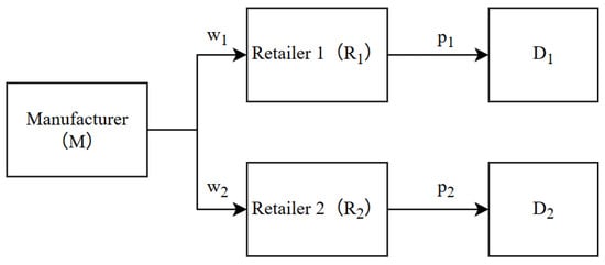
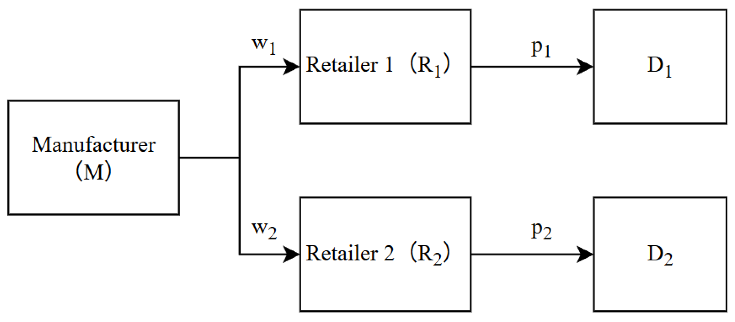
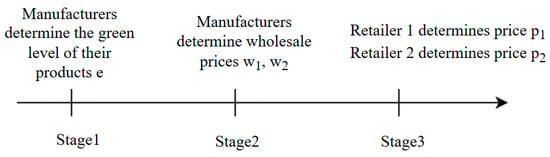
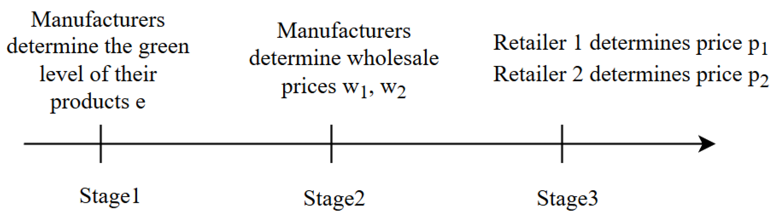
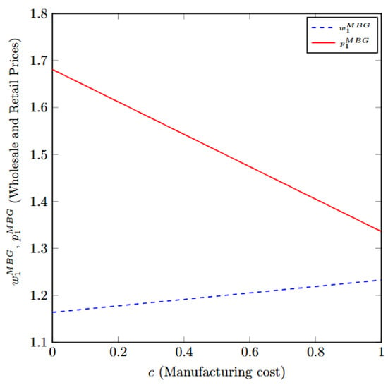
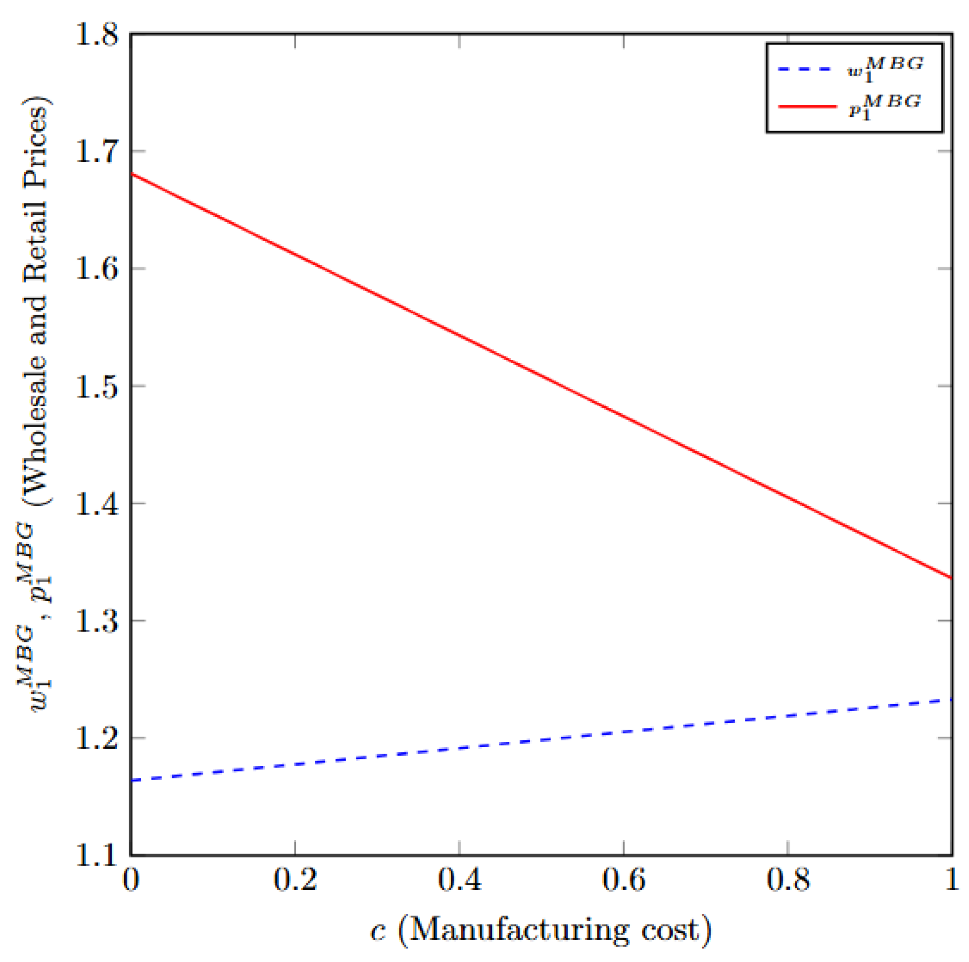
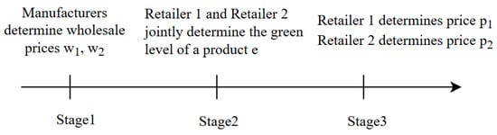
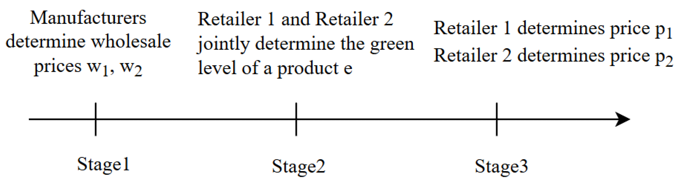
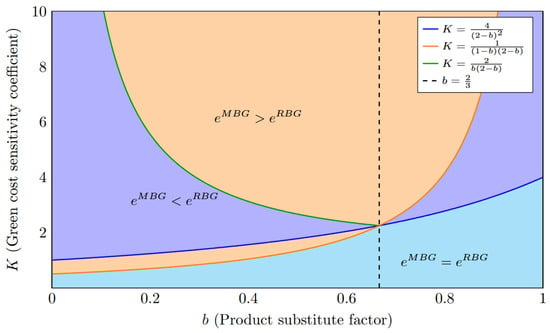
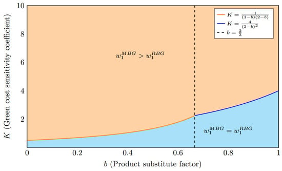
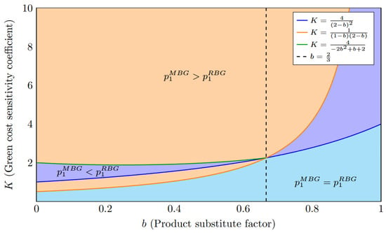
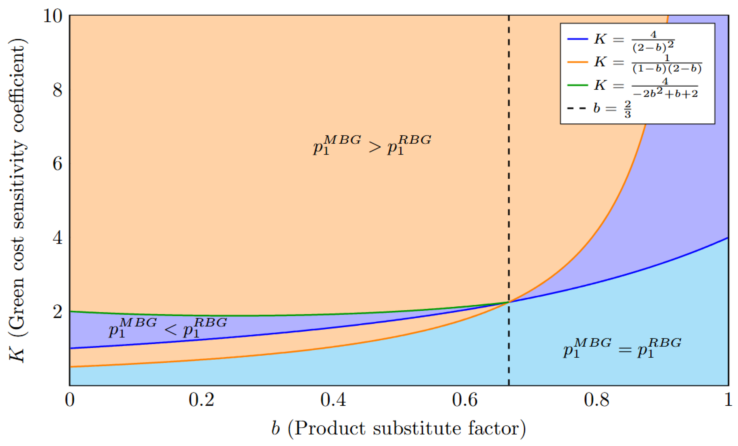
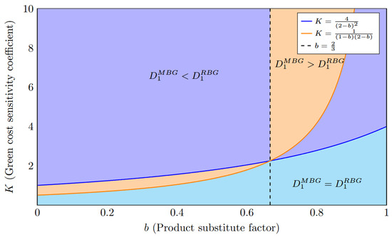
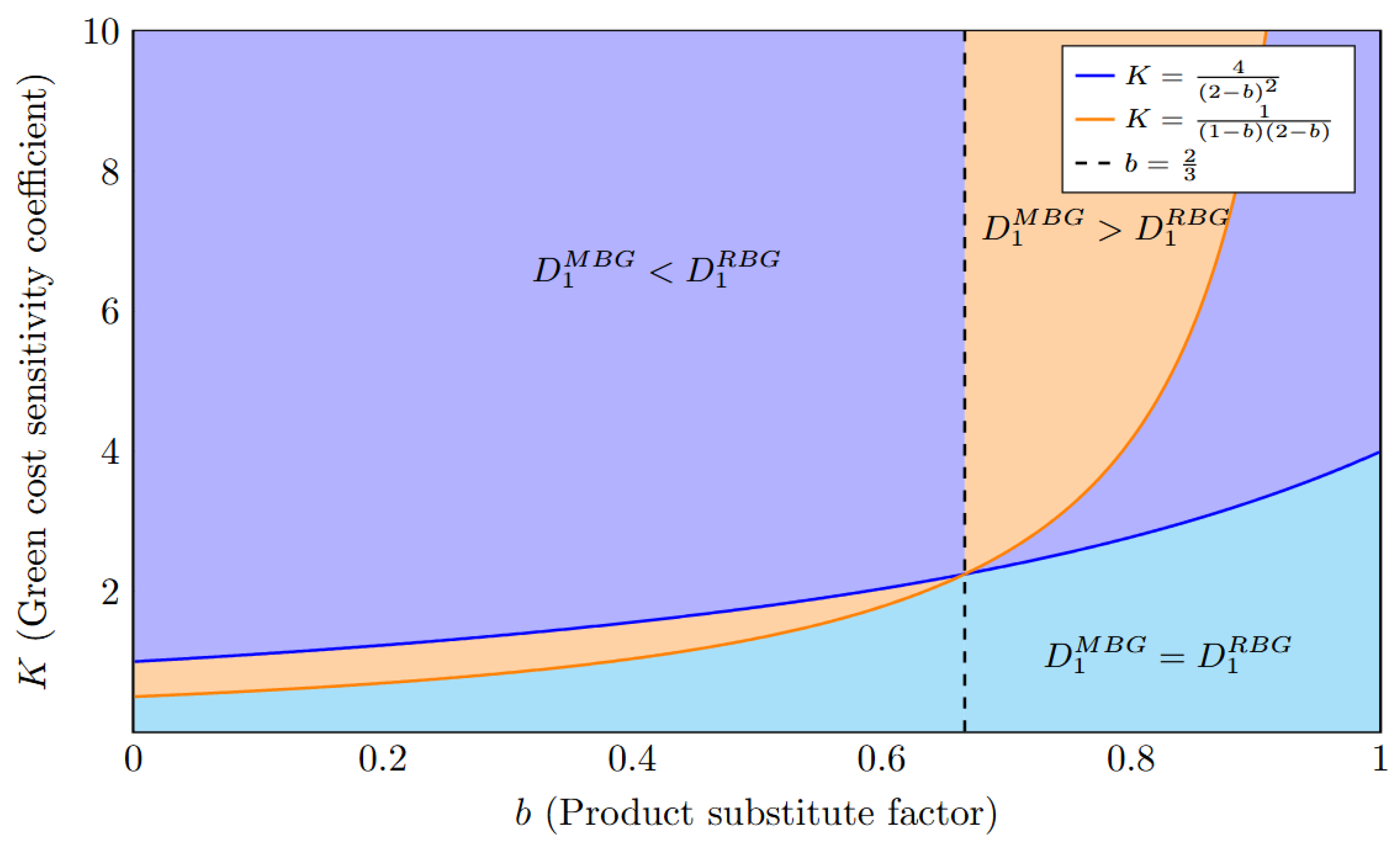
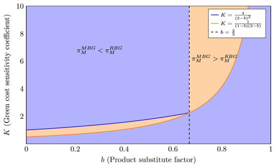
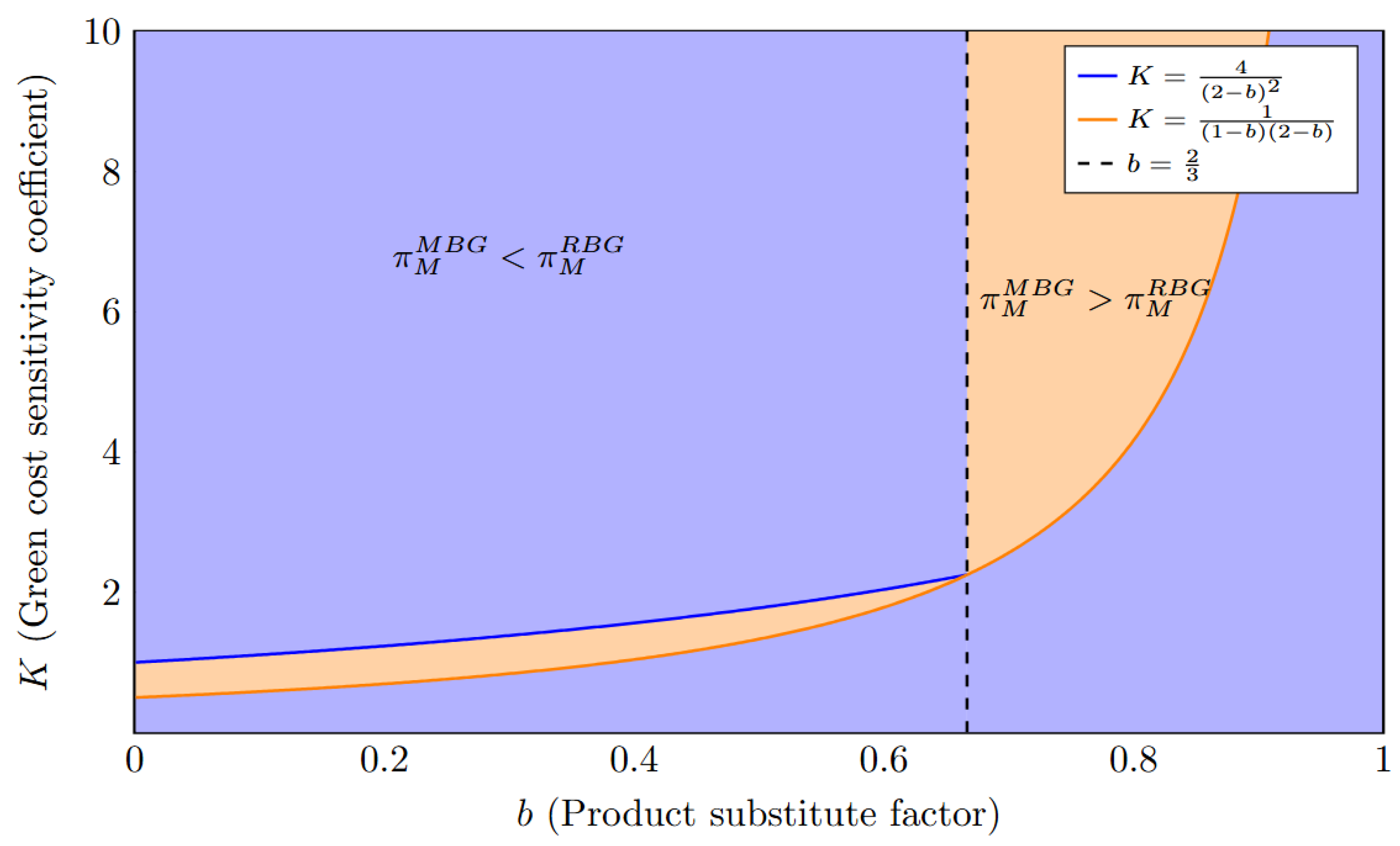
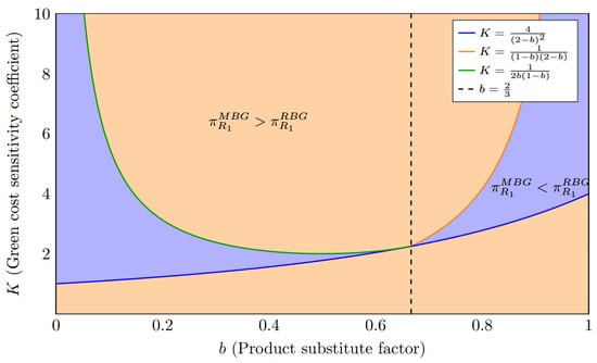
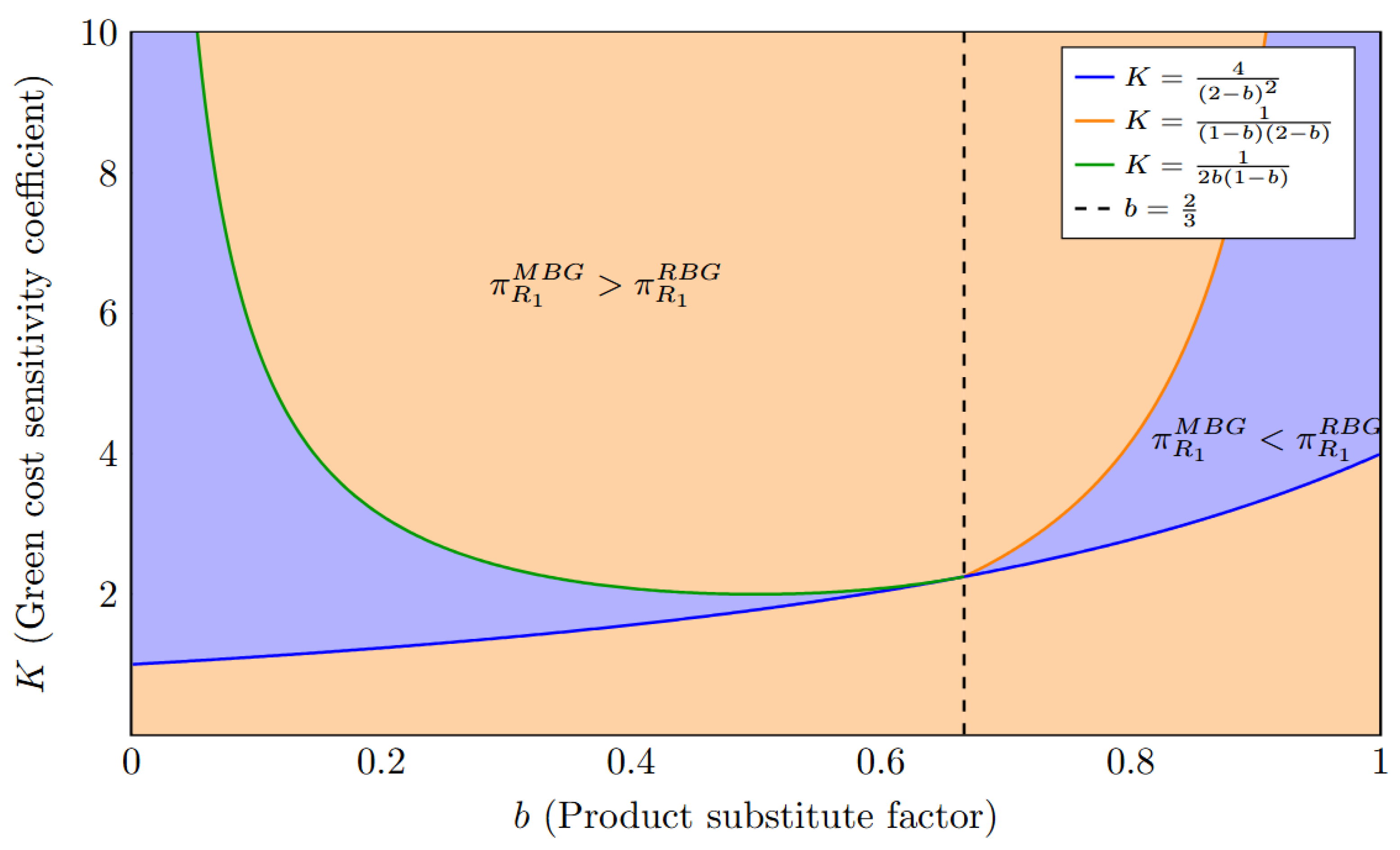

Disclaimer/Publisher’s Note: The statements, opinions and data contained in all publications are solely those of the individual author(s) and contributor(s) and not of MDPI and/or the editor(s). MDPI and/or the editor(s) disclaim responsibility for any injury to people or property resulting from any ideas, methods, instructions or products referred to in the content. |
© 2026 by the authors. Licensee MDPI, Basel, Switzerland. This article is an open access article distributed under the terms and conditions of the Creative Commons Attribution (CC BY) license.