


Abstract
In this study, we develop a stochastic optimal control model for corporate carbon management that synergistically combines emission reduction initiatives with carbon trading mechanisms. The model incorporates two control variables: the autonomous emission reduction rate and initial carbon allowance purchases, while accounting for both deterministic and stochastic carbon pricing scenarios. The solution is obtained through a two-step optimization procedure that addresses each control variable sequentially. In the first step, the problem is transformed into a Hamilton–Jacobi–Bellman (HJB) equation in the sense of viscosity solution. A key aspect of the methodology is deriving the corresponding analytical solution based on this equation’s structure. The second-step optimization results are shown to depend on the relationship between the risk-free interest rate and carbon price dynamics. Furthermore, we employ daily closing prices from 16 July 2021, to 31 December 2024, as the sample dataset to calibrate the parameters governing carbon allowance price evolution. The marginal abatement cost (MAC) curve is calibrated using data derived from the Emissions Prediction and Policy Analysis (EPPA) model, enabling the estimation of the emission reduction efficiency parameter. Additional policy-related parameters are obtained from relevant regulatory documents. The numerical results demonstrate how enterprises can implement the model’s outputs to inform carbon emission reduction decisions in practice and offer enterprises a decision-support tool that integrates theoretical rigor and practical applicability for achieving emission targets in the carbon market.
MSC:
35F21; 49L12; 93E20
1. Introduction
The global climate crisis, intensified by the greenhouse effect, continues to worsen. According to EU climate monitoring data, 2023 was the hottest summer on record since 1940 and marked by frequent extreme weather events, including heat waves, droughts, floods, and wildfires. In response, international treaties such as the UN Framework Convention on Climate Change, the Kyoto Protocol, and the Paris Agreement have been established. In particular, the Kyoto Protocol introduced mandatory carbon emission caps for participating countries, which subsequently set limits for regulated companies. Firms that exceed these limits must either pay penalties or purchase carbon emission allowances (“carbon quotas”), while those that emit less can sell surplus quotas, forming a “carbon trading” mechanism and giving rise to carbon markets. According to ICAP’s Global Carbon Market Progress Report 2025, carbon markets have expanded rapidly since 2014 in both number and coverage, with nearly one-third of the global population now living in regions with active carbon markets (https://icapcarbonaction.com/en/publications/emissions-trading-worldwide-icap-status-report-2025, (accessed on 8 April 2025)). In China, climate action remains a high priority. The Chinese government has committed to peaking carbon emissions before 2030 and achieving carbon neutrality before 2060—targets known as the “dual carbon” goals.
Early mathematical modeling studies of carbon markets primarily focused on trading mechanisms and quota pricing. The theoretical foundation was established by Dales and Montgomery’s tradable permit model for environmental goods [1,2]. Subsequent research involved empirical analyses of carbon quota prices based on carbon market data, such as the studies by Benz and Trück [3] and Koop and Tole [4]. Additionally, several studies explored equilibrium problems in carbon markets, including Seifert et al.’s stochastic model of EU ETS price formation [5] and Carmona et al.’s work on dynamic equilibrium and market design [6]. Building on this approach, researchers further examined the economic mechanisms behind carbon allowance price formation and provided quantitative tools to analyze alternative market designs [7]. Later, Hinz and Novikov [8] developed a risk-neutral pricing model, revealing the disconnect between social optimality and market equilibrium under risk aversion. Moreover, since carbon quota prices exhibit fluctuations similar to financial assets, derivative products based on carbon allowances have emerged. Consequently, Carmona et al. [9] established a system of singular forward–backward stochastic differential equations to study carbon option pricing. For further research on the pricing of carbon emission derivatives, refer to the works of Carmona and Hinz [10] and Çetin and Verschuere [11], among others.
Given the constraints of limited resources, it is crucial for both nations and enterprises to achieve carbon dioxide emission reduction targets in a more efficient and cost-effective manner. Consequently, in another branch of research, stochastic optimal control models related to reducing carbon emissions have been developed from the perspective of production optimization for countries and firms. Zagheni and Billari [12] established a model within the Black–Scholes option-pricing framework to evaluate the cost of a nation’s excess carbon emissions, thereby incorporating the carbon emission problem into a partial differential equation framework. Building upon this work, Yang and Liang [13] introduced a logistic population growth model to enhance the model’s realism. Subsequently, within Merton’s consumption framework [14,15], they incorporated control factors into the contingent claim-pricing model to formulate the optimal control problem for reducing carbon emissions. Later, Yang et al. [16] developed two models based on distinct emission reduction strategies within a stochastic optimal control framework. Furthermore, Guo and Liang [17,18] extended the work of [13] by integrating carbon trading mechanisms and assuming that market carbon allowance prices follow geometric Brownian motion. In addition, many studies have been conducted from the perspective of optimizing the cost of reducing enterprise emissions. Taking an example from the literature [19], Liang et al. considered the existence of the carbon market. At the time of verification, an enterprise can purchase carbon quotas to compensate for its own shortage of quotas instead of accepting an excessive penalty. Meanwhile, if an enterprise has remaining carbon quotas, they can sell for profit. The enterprise can optimize the cost of reducing emissions by controlling its internal emission reduction rate and initial quantity of carbon quotas purchased. Based on this information, they established an optimal stochastic control model for the enterprise and conducted theoretical research on the corresponding Hamilton–Jacobi–Bellman (HJB) equation through viscosity solutions. On this basis, Huang [20] discovered that the HJB equation in [19] is actually a semi-linear partial differential equation with bounded coefficients, which can prove the existence and uniqueness of its classical solution. Recently, Huang et al. [21] also considered a model that simultaneously optimizes two control factors, namely, the emission reduction strategy and the initial volume of carbon quotas purchased. They studied the classical solutions of the model and discussed the existence and uniqueness of the optimal strategy. Aïd and Biagini [22] have addressed similar problems in a more complex framework. By employing variational methods, the authors derive a closed-form market equilibrium that is contingent upon the regulator’s dynamic allocation strategy. Wang et al. [23] further incorporated environmental noise into the system by proposing a stochastic carbon emission model. Their findings demonstrate that effective mitigation strategies must balance ecological sustainability with economic feasibility. However, these studies primarily focus on theoretical properties and often rely on numerical solutions for practical applications.
To address barriers to the practical application of existing carbon emission reduction models, particularly those in [19,21], this study focuses on overcoming their reliance on numerical methods. Although prior research established relatively comprehensive theoretical frameworks, such as analyses based on classical and viscosity solutions, their practical implementation remains dependent on numerical approaches, which limits the intuitiveness of model outputs and constrains decision-support capabilities. Therefore, the objective of this study is to derive an analytical solution for the model, enabling enterprises to directly utilize the resulting explicit formulas to determine optimal emission reduction strategies. Fortunately, we observe that the state variables in the proposed model evolve linearly, while the objective function takes a quadratic form. This structure is that of a Linear–Quadratic (LQ) control problem [24], which enables the derivation of an analytical solution. This approach is expected to yield two major breakthroughs: First, it will transform optimal emission reduction strategies into clear decision rules, enabling enterprises to directly compute optimal strategies based on their specific parameters—much like applying a formula—without resorting to complex simulations. Second, through analytical expressions, it will explicitly reveal the direct influence of key parameters (such as carbon price and technology cost) on optimal strategies, thereby significantly enhancing the model’s transparency, interpretability, and practical operability. Ultimately, this study provides enterprises with a carbon management decision-support tool that integrates theoretical rigor with practical guidance. Therefore, based on the research in [19,20,21], we continue to examine the issue of optimal control of carbon emission reduction in an enterprise. In our model, the enterprise can optimize the cost of reducing emissions by controlling its internal emission reduction rate and initial quantity of carbon quotas purchased. The model is developed under two distinct carbon pricing scenarios: deterministic and stochastic. Through stochastic control theory, the model is transformed into an HJB equation in the sense of the viscosity solution. In fact, the HJB equation, also referred to as the dynamic programming equation, represents the infinitesimal version of the dynamic programming principle. This principle, originally introduced by Bellman in 1957 [25], provides a foundational methodology for solving stochastic optimal control problems. Given that the model presented in this paper incorporates stochastic disturbances, such as those affecting carbon emission levels and carbon prices, it becomes essential to employ the HJB equation. This approach transforms the complex problem of identifying an optimal control trajectory into the task of determining a scalar-valued function, which subsequently yields an optimal feedback control law in closed form. Consequently, solving the HJB equation within our model constitutes a critical step toward deriving an explicit analytical solution. According to the structural characteristics of the equation, its analytical solution can be obtained. Therefore, the explicit expression of the enterprise’s optimal emission reduction strategy can be obtained. Finally, the numerical results collectively demonstrate the model’s practical utility and provide actionable insights for carbon market participants.
In summary, although existing studies have established relatively comprehensive theoretical frameworks for carbon emission reduction from perspectives such as classical and viscosity solutions, their practical application typically relies on numerical solutions. By deriving explicit analytical solutions, this study facilitates, to a considerable extent, enterprises’ direct utilization of model outputs for carbon reduction decision-making, thereby enhancing operational feasibility in practical implementation.
The remainder of this paper is organized as follows: In the next section, we establish models under both deterministic and stochastic carbon price scenarios. In Section 3, we prove that the value function generated by this optimization problem is the unique viscosity solution of the corresponding HJB equation. In Section 4, we present the analytical solutions to the optimal emission control problem under both scenarios. Section 5 demonstrates the model’s numerical results and practical implications. Section 6 concludes the paper by summarizing the main findings and their implications.
2. Model
Let be a filtered probability space that satisfies the usual conditions. Suppose, in the period , an enterprise emits carbon dioxide through its production activities and is required to reduce its emissions. At time , the enterprise obtains carbon quotas of tons freely from the government and tons by purchasing them on the carbon market, where is given and is undetermined. Let represent the carbon quota price on the carbon market at time t. In the following sections, we will discuss its evolution in two scenarios: deterministic and stochastic. Define as the firm’s expected cumulative emissions within at time t. Thus, at time T, is equal to the accumulated carbon dioxide emissions of the enterprise within the time period . The formulation of the expected cumulative carbon emission process X is motivated by that in [5,21]. Suppose the process is satisfied by
where the control is a progressively measurable (with respect to ) process, representing the instantaneous emission reduction rate. We denote by the set of admissible control processes u such that , where M is a sufficiently large, fixed positive constant. The existence of such an M ensures that the optimization problem is well-posed over a non-empty set of controls with finite second moments. is the standard Brown motion, and is a smooth function of time t with a positive lower bound, representing the volatility. In this model, the impact of reducing emissions on production and profit is not considered. That is, through reducing its emissions, the enterprise only reduces the amount of carbon dioxide emitted per unit of production.
At verification time T, if the total carbon dioxide emissions of the enterprise exceed the prescribed limit, that is, the allowable emissions, the enterprise needs to purchase additional carbon quotas on the market. The permitted emissions consist of two parts: The first part is the free permitted quota issued by the government at the initial time, , and the second is the emission quota purchased by the enterprises at the initial time, . If the limit is not exceeded, the remaining part can be sold on the carbon market for profit. Therefore, the total expected cost at the initial moment is
where the parameter denotes the discount rate, and represents the per-unit-time cost for the company to implement emission reduction strategies, which is a function of the reduction rate. We assume that , where m is a positive constant and reflects the emission reduction efficiency. The choice of a quadratic form for the function is in line with the literature on carbon emission reduction (see Yang et al. [16], Gollier [26], and the references therein). In ref. [16], the authors used actual data to fit the emission reduction cost function and found that the quadratic function had the best fitting effect, and in ref. [22], the authors emphasized that the quadratic form captures the nondecreasing feature of the marginal abatement cost. From an investment point of view, it means that there is some irreversibility in the abatement decision. Furthermore, according to the definition of the state variable in (1), its uncertainty originates from the stochastic term , which represents the increment of a Wiener process and follows a normal distribution with a mean of 0 and a variance of . Therefore, the expectation in (2) is adopted with respect to this normal distribution.
The right-hand side of the Equation (2) consists of three cash flow components: The first term accounts for the expenses incurred due to emission control measures during the interval . The second term reflects the cost or revenue associated with carbon allowances. If the cumulative emissions exceed the cap , the company must purchase additional allowances at price . Conversely, if falls below the limit, the company can earn revenue by selling surplus allowances at . The third term represents the initial cost of purchasing emission quotas at time .
Suppose the company’s goal is to minimize the total cost of reducing emissions by optimizing the emission reduction control strategy u and the initial amount of carbon quotas purchased, , that is, to find the optimal control strategy and the optimal purchase amount such that
Referring to the result in [21], for all , we can prove that
holds. See Theorem A1 in Appendix A for the specific proof. Therefore, we can optimize the problem (3) in two steps. In the following sections, we will solve the aforementioned optimization problem for two distinct scenarios: deterministic and stochastic carbon allowance prices.
2.1. Case 1: Deterministic Carbon Allowance Price
In this section, we consider the case in which the carbon allowance price is deterministic, specifically modeling the price as a time-varying function . The total expected cost at the initial moment is
Therefore, according to (4), we can decompose the aforementioned optimization problem into a two-step solution procedure.
Step 1: Fix and find the optimal emission reduction control strategy such that .
Let
Then,
Thus, in order to find , we need to solve . According to the dynamic programming principle [27], we will prove in the next section that the value function is the unique viscosity solution of the following HJB equation:
In fact, the theory of viscosity solutions [27,28] was a major breakthrough in the analysis of HJB equations, as it relaxes the smoothness requirements for V. This framework allows the value function V to be defined as a “generalized solution” of the HJB Equation (7), even when it is not differentiable everywhere. Therefore, within the viscosity solution framework, we can transform the stochastic optimal control problem into solving an HJB equation. Moreover, since we derive an analytical solution, specifically, a classical solution, to this HJB Equation (7) in subsequent analysis, it naturally recovers the original value function V.
Since is equal to according to the previous definition, satisfies . Thus, letting , we can obtain . Therefore, the optimal emission reduction strategy can be obtained as follows:
That is to say, once we have obtained the value function V, the corresponding optimal feedback control can also be obtained.
Step 2: With the solution of Step 1, find the optimal purchase amount .
The total cost is
Therefore, the optimal auction amount is the minimum point of the function about .
2.2. Case 2: Stochastic Carbon Allowance Price
In the previous section, we discussed a simplified scenario in which the carbon allowance price follows a deterministic function for formulating corporate emission reduction strategies. However, actual market conditions demonstrate that carbon allowance prices typically exhibit stochastic fluctuations. Here, we assume that the price follows a geometric Brownian motion, i.e.,
where and are constant drift and volatility terms, respectively, and and are mutually independent. Similar assumption can be found in [19,20,21].
Since the carbon allowance price now follows a stochastic process, compared to the deterministic case discussed in the previous section, the model’s state variables will gain an additional dimension. Consequently, the total expected cost at the initial time can be reformulated as follows:
Similarly, we can decompose the aforementioned optimization problem into a two-step solution process.
Step 1: Fix , find the optimal emission reduction control strategy , such that .
Let
Then,
Thus, in order to find , we need to solve the value function .
According to the dynamic programming principle [27], we will prove in the next section that the value function is the unique viscosity solution of the following HJB equation:
Following a derivation procedure analogous to that of (8) in the deterministic carbon pricing model, the optimal emission reduction strategy can be obtained as
Step 2: With the solution of Step 1, find the optimal purchase amount . Similar to the analysis in the deterministic model, the total cost is
Therefore, the optimal auction amount is the minimum point of the function about .
3. Existence and Uniqueness of the Viscosity Solution
Based on the above analysis, we recognize that the key to solving the aforementioned stochastic optimal control problem lies in determining the value function V. According to the classical dynamic programming principle, we can establish, within the framework of viscosity solutions, an equivalence between the value function and the corresponding HJB equation. Specifically, the value function is the unique viscosity solution of the associated HJB equation. Consequently, solving the stochastic control problem can be transformed into solving the HJB equation.
In the following, we take the case with a stochastic carbon price as an example and prove that the value function defined in (12) is the unique viscosity solution of the HJB Equation (13). As for the case with a deterministic carbon price, the corresponding HJB Equation (7) becomes one-dimensional, which is simpler compared to the two-dimensional case of (13). Therefore, its proof can be derived by reference to the proof for the two-dimensional case, and we will not elaborate on it further here. The proof follows a standard structure in stochastic control theory: we first show continuity and growth properties of V (Propositions 1–3), then verify that it satisfies the viscosity solution definition (Theorem 1), and finally prove uniqueness via a comparison principle (Lemma 1, Theorem 2). The key idea is that even if V is not differentiable everywhere, the viscosity solution framework allows us to work with its sub- and super-differentials, which carry the necessary first-order condition information for optimality.
To simplify notation, we abbreviate to . We now turn to an analysis of the properties of the value function .
Proposition 1.
is a non-decreasing function of x for all , .
Proof.
Let
For any control , initial time , and initial state x, the emission process (with ) is defined accordingly. Suppose , we then have . According to (16), for all , we have
Thus,
□
Proposition 2.
Throughout the domain , is continuous.
Proof.
We first establish the continuity of in the variable x, which holds uniformly for . For fixed , there exist controls for any satisfying
It follows from Proposition 1 that
Then
, we have
where, for , the term represents the expectation at time T for the process X defined in (1), starting from the initial condition .
According to the estimates of the moments for the stochastic differential equations (SDEs) [27], and
we have
where is a positive constant. Then
We now proceed to demonstrate the continuity of with respect to s, uniformly over t. For fixed parameters and any ordered pair , there exist admissible controls such that
Similar to the previous one, we have
Then, for all ,
where, for , represents the expectation at time T of process S in (10) with initial condition . is a positive constant. Then
We proceed to demonstrate that is continuous in t. Given fixed , for all with , the dynamic programming principle [27] gives
where is a positive constant. Since V is Lipschitz in uniformly in t and from the estimates of the moments for the SDEs [27], we have
where , , are positive constants. Thus,
□
Proposition 3.
exhibits at most quadratic growth. That is, for any , there exists , such that .
Proof.
From (12), for any , we have
Moreover, under any admissible control and initial condition , each of the SDEs (1) for and (10) for possesses a unique strong solution. Thus, according to [29], there exists and , such that
□
In the following, we prove the existence of the viscosity solution for our problem, referring to [27,28].
Proof.
Having established the continuity of , we also note that it clearly satisfies the terminal condition.
We now prove that is a viscosity subsolution of Equation (13). Consider a test function and a point at which attains a local maximum with . By definition, this implies the existence of a neighborhood wherein the inequality holds. Corresponding to the initial state and a control , let solve (1) and (10). We introduce the stopping time . Then, for and any constant control , it follows from the dynamic programming principle [27] that
Apply It ’s formula to , we can obtain
Plugging this into the preceding inequality yields
Multiplying both sides by and then taking the limit as yields
By the arbitrariness of u, we have
Hence, constitutes a viscosity subsolution of (13).
We now turn to proving that is a viscosity supersolution of (13). Similarly, let be a test function, and suppose is a local minimum point of with . This implies the existence of a neighborhood such that for all . Consider the solution of (1) and (10) starting from under control , and introduce the stopping time . Applying the dynamic programming principle [27], we obtain that for all there exists an admissible control with the property that
where , the processes and are the corresponding solutions of (1) and (10) under the control . Then, applying Itô’s formula to the expression , we obtain
This leads to the following inequality upon substitution:
Since
It has thus been proven that is a viscosity supersolution, and hence a viscosity solution, of Equation (13). □
Having established that the value function is a viscosity solution, we proceed to prove a comparison principle for this problem. This, in turn, will imply the uniqueness of the viscosity solution.
Setting , , , we have
Lemma 1
Proof.
Suppose otherwise, it would follow that there exists a point and a constant satisfying
where . Otherwise (i.e., if ), due to the continuity of U and V, condition (20) can be satisfied at some point near . We now introduce the following auxiliary function
where and
Let
Due to the polynomial growth bound and the semi-continuity of U and V, it follows that admits a maximum point, which we denote as , i.e.,
Provided that is sufficiently small, the following holds:
Since , we then have
That is
Since
we then have
where is a positive constant. The preceding equation yields positive constants and satisfying , and , which ensures the boundedness of . For any fixed , this sequence has a convergent subsequence (without relabeling) whose limit we denote by . Furthermore, the existence of a constant such that implies that and tend to zero as . Hence, at the limit point, and , we accordingly set and .
According to , then
Let , we have
Were it the case that , taking the limit and invoking the terminal inequality would yield , contradicting our initial assumption. Thus, , and so for sufficiently large , the points and belong to . An application of the Crandall–Ishii lemma (detailed in [28], Chapter V, Theorem 6.1), then provides the existence of , , p, , M, N satisfying , , i.e., belonging to the superdifferential of V and the subdifferential of U at the respective points and
Given that V is a viscosity subsolution and U is a supersolution, a control can be chosen satisfying
Subtracting the two equations yields
Setting , we have
Let
Choose sufficiently large so that . We now consider two cases for : in the case where and , we have ; if either or , we may pick small enough so that . Combining these estimates leads to . Thus we reach a contradiction, refuting the original hypothesis and proving that for all . □
An immediate consequence of the comparison principle is:
4. Analytic Solution
Within the framework of viscosity solutions, we have transformed the aforementioned stochastic optimal control problem into solving the HJB equation. That is to say, if we can obtain an analytical solution (classical solutions are naturally also viscosity solutions) to the HJB equation, then we can derive the corresponding value function. Therefore, we will next attempt to derive explicit expressions for the solutions of HJB Equations (7) and (13).
4.1. Case 1: Deterministic Carbon Allowance Price
Since the state variables in the proposed model evolve linearly, while the objective function takes a quadratic form, this structure is a Linear–Quadratic (LQ) control problem, which enables the derivation of an analytical solution. Based on the structure of Equation (21), we conjecture that its solution should be of a linear form, i.e.,
where and are undetermined parameters. Substituting (22) into (21), we obtain
Solving the aforementioned two ordinary differential equations, we obtain
Since
This indicates that is a monotonic function of . Therefore, when , monotonically increases with —in other words, if the initial carbon allowance price is higher than its discounted present value at the verification time—the enterprise should minimize purchases at the initial time (i.e., ) to achieve the lowest total cost. Conversely, when , monotonically decreases with , it implies that if the initial carbon allowance price is lower than its discounted present value at the verification time, the enterprise should purchase as much as possible at the initial time to minimize the total cost.
4.2. Case 2: Stochastic Carbon Allowance Price
For the stochastic carbon price case, according to the two-step optimization in Section 2, the key to solving this optimization problem lies in solving the HJB Equation (13). Substituting (14) into (13), we have
This is also a LQ control problem. Therefore, based on the structure of (28), we conjecture that its solution admits the following quadratic form:
where , and are undetermined parameters. Substituting (29) into (28), we obtain
Solving the aforementioned three ordinary differential equations, we obtain
Therefore,
From (14), the optimal control strategy can be derived as
Furthermore, we find the optimal purchase amount . Similar to the analysis in the deterministic model, the total cost is
Since
This indicates that is a monotonic function of . Therefore, when , i.e., , monotonically increases with . In other words, if the expected growth rate of the carbon allowance price is lower than the risk-free interest rate, the enterprise should minimize purchases at the initial time (i.e., ) to achieve the lowest total cost. Conversely, when , i.e., , monotonically decreases with . This implies that if the expected growth rate of the carbon allowance price is higher than the risk-free interest rate, the enterprise should purchase as much as possible at the initial time to minimize the total cost.
5. Numerical Results and Practical Implications
In previous sections, we determined the minimum total emission reduction cost and optimal mitigation strategy by solving Equations (7) and (13). This section is designed to transform the aforementioned theoretical model into a decision support tool that can be directly utilized by carbon market participants. We begin with a detailed description of how to calibrate model parameters using publicly available and market data. Subsequently, we employ numerical simulations to demonstrate how key market variables influence firms’ optimal strategies. Finally, we distill specific actionable guidelines for carbon market participants.
5.1. Parameter Calibration
The first step for enterprises to apply this model is parameter calibration. Based on actual data from China’s carbon market, we provide a comprehensive parameter setting guide (summarized in Table 1), which can be directly applied or adapted by companies. In the stochastic carbon allowance pricing model, there are six key parameters to be determined: the emission reduction efficiency parameter m, the compliance period T, the risk-free interest rate r, the drift term and diffusion term of the price of carbon allowance, and the government-allocated free carbon allowance quota . Specifically, similar to [16], the marginal abatement cost (MAC) curve can be fitted through the data obtained from the Emissions Prediction and Policy Assessment (EPPA) model, so as to obtain the value of the emission reduction efficiency parameter m. We refer to the fitting results of the emission reduction cost curve in [16] to select the parameter . In accordance with the current policy of China’s carbon emission trading market (https://www.kwm.com/cn/zh/insights/latest-thinking/focus-on-carbon-trading-development-and-current-situation-of-carbon-emission-trading-market.html, (accessed on 31 December 2024) (In Chinese)), the compliance period for emission-regulated enterprises is one year. Therefore, we select the parameter . Furthermore, since all enterprises are allocated a carbon emission allowance of 10,000 tons (https://esg.cueb.edu.cn/article/p-173.html, (accessed on 31 December 2024) (In Chinese)), we set . The risk-free rate r can be set as the current yield of China’s 10-year government bonds, given its current annualized yield of 1.68% (https://quote.eastmoney.com/stock/171.CN10Y.html, (accessed on 31 December 2024) (In Chinese)), the equivalent daily rate is approximately calculated as . Following the methodology in [30], we determine the drift term and diffusion term for the carbon emission allowance (CEA) prices. Since trading on China’s national carbon market commenced 16 July 2021, we employ the daily closing prices of CEA from 16 July 2021, to 31 December 2024 as the sample dataset. (Note on Data Recency: The parameter calibration in this study utilizes historical data up to 31 December 2024, which corresponds to the latest complete and verified dataset available at the time of this research. The model framework is designed to be forward-looking, and its parameters can and should be updated as new market data becomes available. Future applications of this model are encouraged to incorporate data from 2025 and beyond to ensure the inputs reflect the most current market conditions. The analytical nature of the solution makes such periodic re-calibration a straightforward task for practitioners.) Specifically, the drift term is estimated as the mean logarithmic return of the CEA prices. The volatility term is derived by fitting an ARMA(2,2)-GARCH(1,1) model to the log-return series of the CEA prices. This approach effectively captures the clustering of volatility and time-varying characteristics of carbon market risk. To ensure the model specification is adequate and that the estimated volatility is reliable, we report the key diagnostic tests on the standardized residuals as conducted in [30]. The Ljung–Box tests on both the residual series and the squared residual series showed no significant autocorrelation up to 20 lags (p-values > 0.1), and the ARCH-LM test indicated no remaining ARCH effects (p-value > 0.1). These results collectively suggest that the standardized residuals approximate a white noise process. This validates that the chosen ARMA-GARCH model has sufficiently captured the linear and non-linear dependencies in the price dynamics, thereby providing a reliable and robust estimate for the volatility parameter used in our stochastic control model. Based on the results in [30], we set , . Thus, , based on the previous discussion of (32), the enterprise should purchase as much as possible at the initial time to minimize the total cost. Subject to relevant policies (https://www.cets.org.cn/gpxyjy/index.jhtml, (accessed on 31 December 2024) (in Chinese)), there is an upper limit on the transaction amount, denoted as = 100,000. Therefore, the optimal purchase amount = 100,000. In the deterministic carbon allowance pricing model, for simplicity, we can assume the time-varying price function satisfies (10) with , i.e., . Consistent with the stochastic model, we set .
Table 1.
Guidelines for Model Parameter Calibration and Reference Values.
5.2. Sensitivity Analysis
Next, we will substitute the selected parameter values mentioned above into the expressions derived in Section 3 and Section 4 to calculate the corresponding optimal abatement strategies and optimal costs, and conduct sensitivity analysis on the parameters.
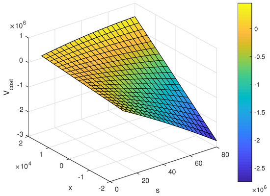
Figure 1 illustrates the minimum total emission reduction cost for the firm in the context of stochastic carbon allowance prices. The total cost increases with higher expected carbon emissions. Notably, when the initial expected emissions are low, rising carbon prices lead to reduced total costs or even increased profits. This occurs because the firm is more likely to hold surplus allowances when it is evaluated for compliance, which can be sold on the carbon market for higher prices, thus increasing revenue. Conversely, when initial expected emissions are high, increasing carbon prices drive up total costs. In this scenario, the firm is more likely to exceed its allowance quotas and purchase additional allowances to maintain compliance, resulting in cost escalation proportional to price rises.
Figure 1.
Total cost under stochastic carbon allowance prices.
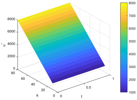
Figure 2 presents the optimal emission reduction rate for the firm under stochastic carbon allowance prices. As shown in the figure, at any given time point, the optimal emission reduction rate increases with rising carbon allowance prices. This occurs because both the cost of purchasing additional allowances and the revenue from selling surplus allowances increase with higher allowance prices at the time of the compliance evaluation. Consequently, to minimize costs or maximize profits, the firm should reduce emissions as much as possible. Furthermore, when the carbon allowance price remains constant, the optimal emission reduction rate for the firm increases progressively as the compliance deadline approaches.
Figure 2.
Optimal emission reduction rate under stochastic carbon allowance prices.
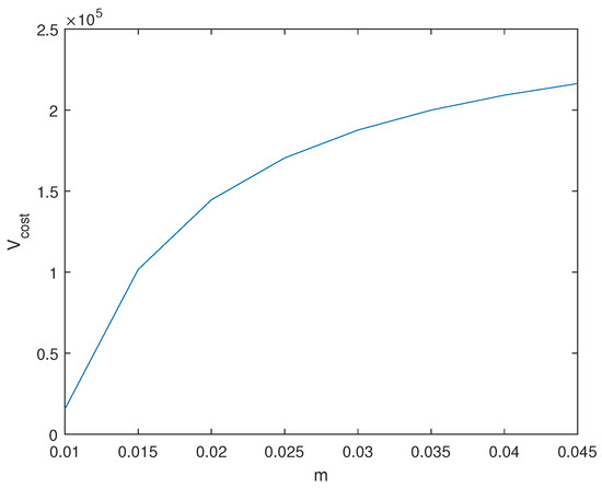
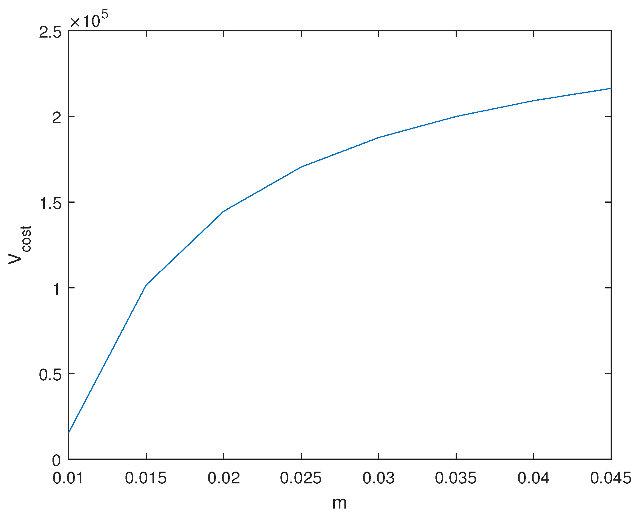
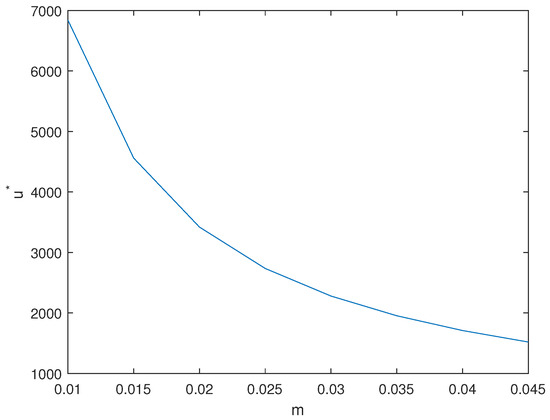
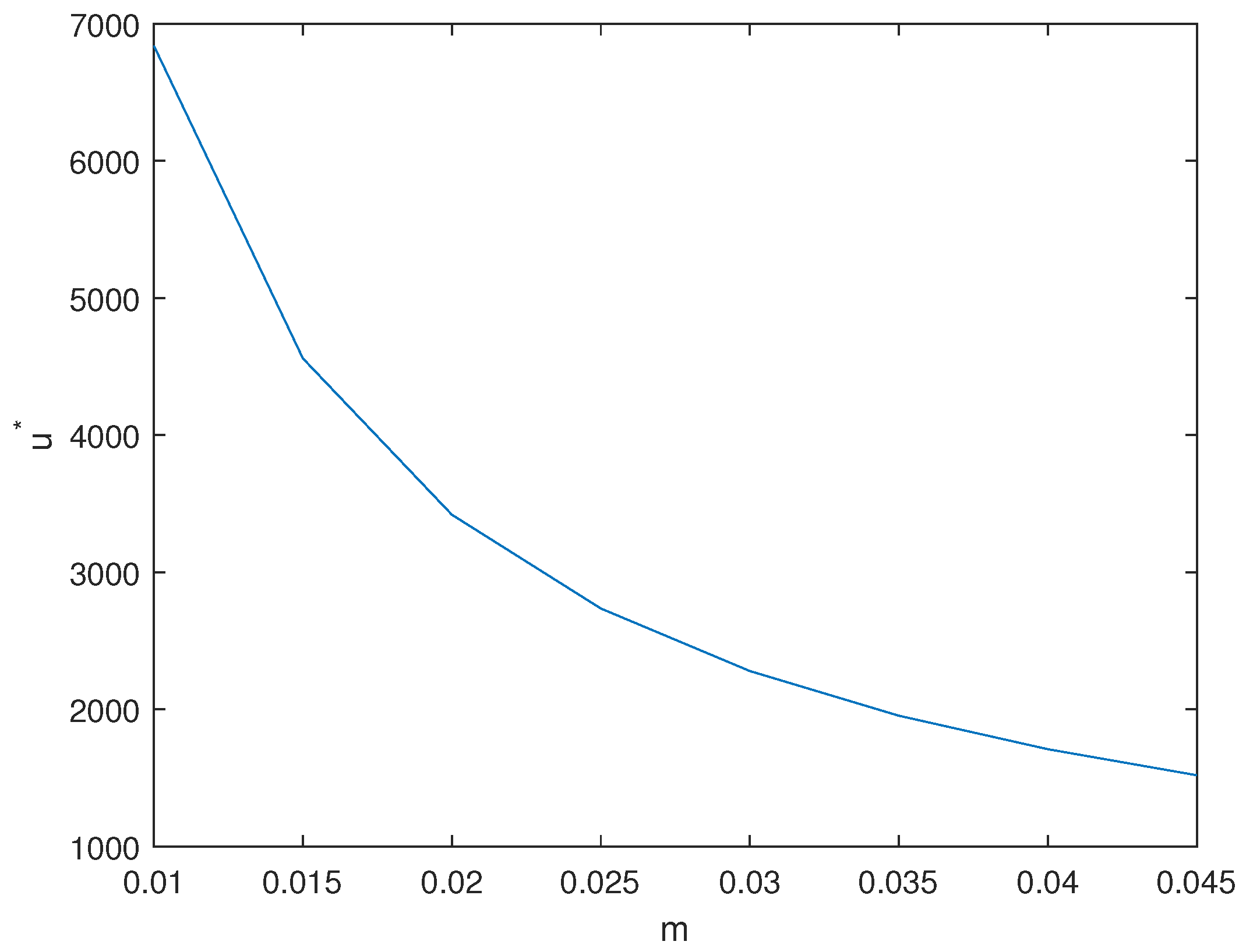
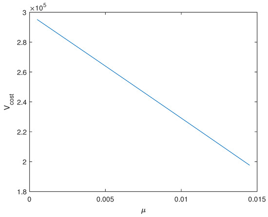
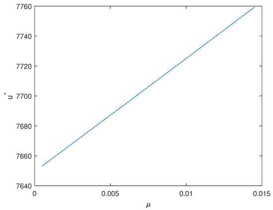
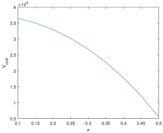
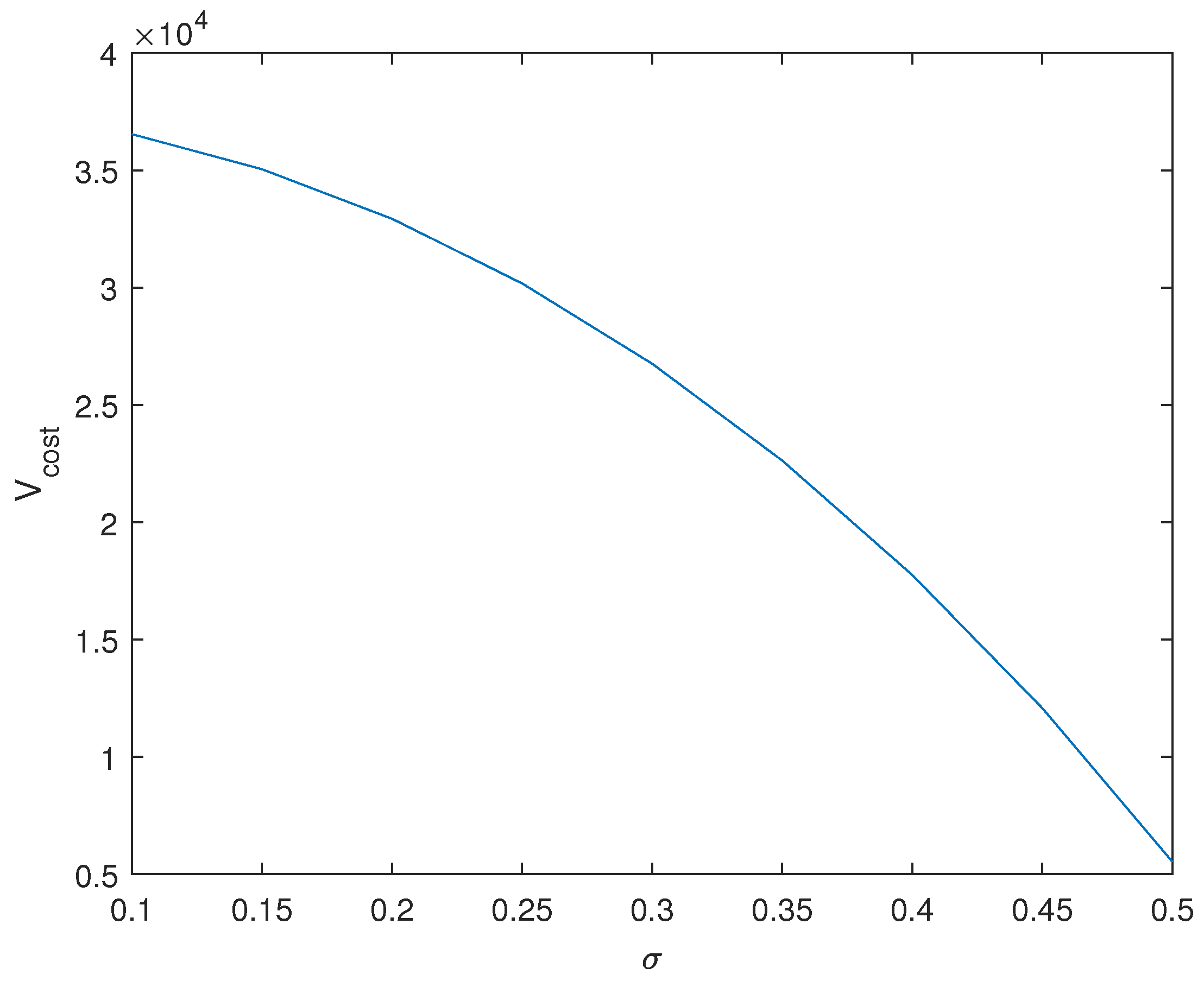
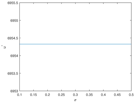
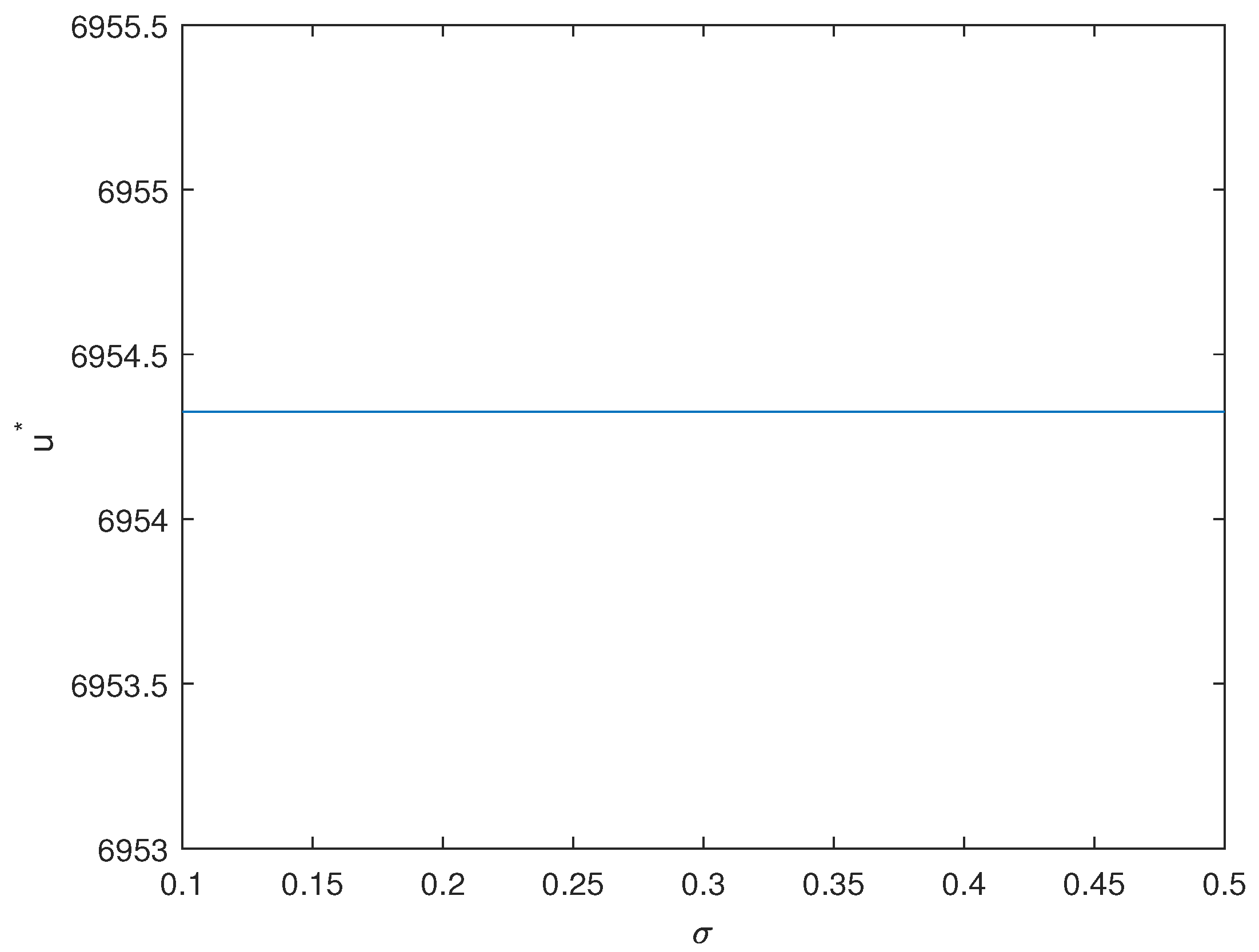
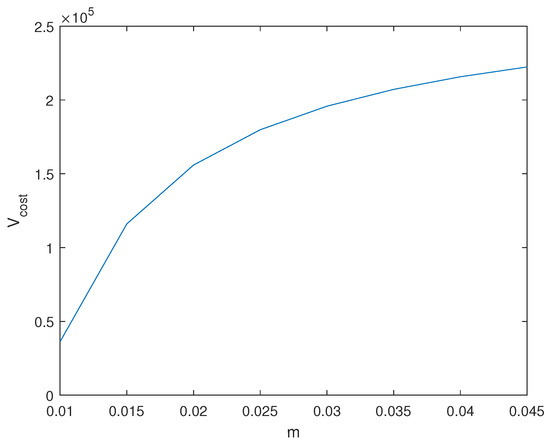
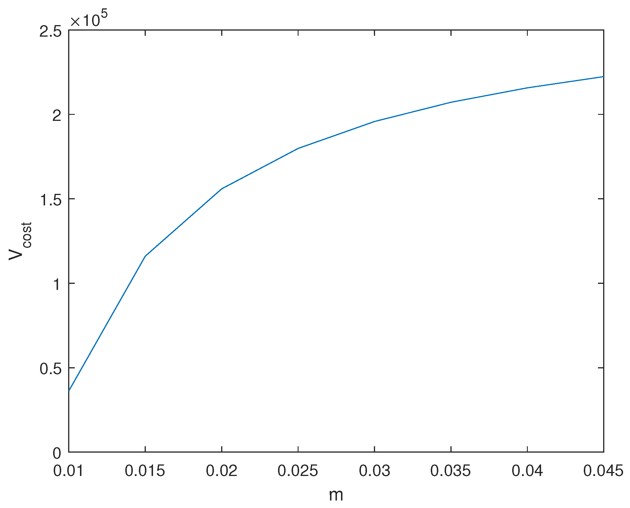
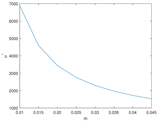
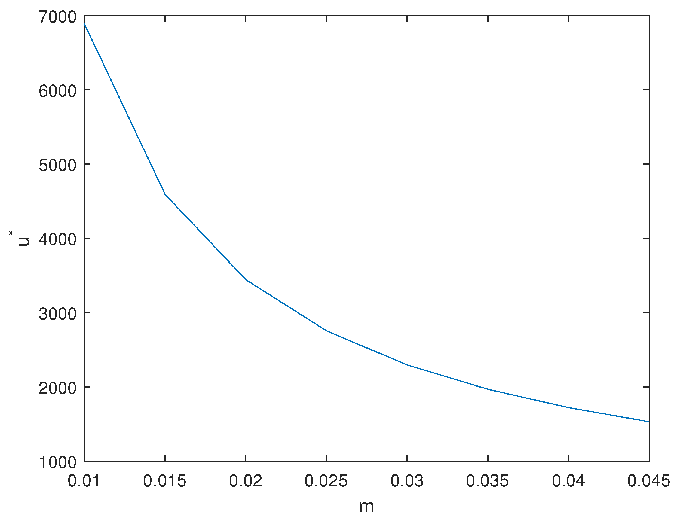
Figure 3, Figure 4, Figure 5, Figure 6, Figure 7 and Figure 8 illustrate the relationships between the minimum total cost, optimal emission reduction rate, and various parameters. As shown in Figure 3, the total cost increases with m. This is because a larger m leads to higher unit emission reduction cost, thereby increasing the total cost and consequently resulting in a decreasing optimal emission reduction rate, as demonstrated in Figure 4. Figure 5 indicates that as the expected growth rate of carbon allowance prices rises, the total cost decreases accordingly. This occurs because the revenue from selling surplus carbon allowances at the verification moment would increase. Correspondingly, Figure 6 shows that the increase in the expected growth rate of carbon allowance prices raises the cost of purchasing allowances, prompting the enterprise to enhance its emission reduction efforts to lower costs, thus leading to an increase in the optimal emission reduction rate. Figure 7 and Figure 8 present the trends of the minimum total cost and optimal emission reduction rate with respect to the volatility () of the carbon allowance price, which are consistent with the findings in (31) and (32).
Figure 3.
Total cost under stochastic carbon allowance prices with m.
Figure 4.
Optimal emission reduction rate under stochastic carbon allowance prices with m.
Figure 5.
Total cost under stochastic carbon allowance prices with .
Figure 6.
Optimal emission reduction rate under stochastic carbon allowance prices with .
Figure 7.
Total cost under stochastic carbon allowance prices with .
Figure 8.
Optimal emission reduction rate under stochastic carbon allowance prices with .
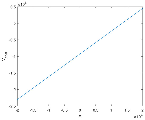
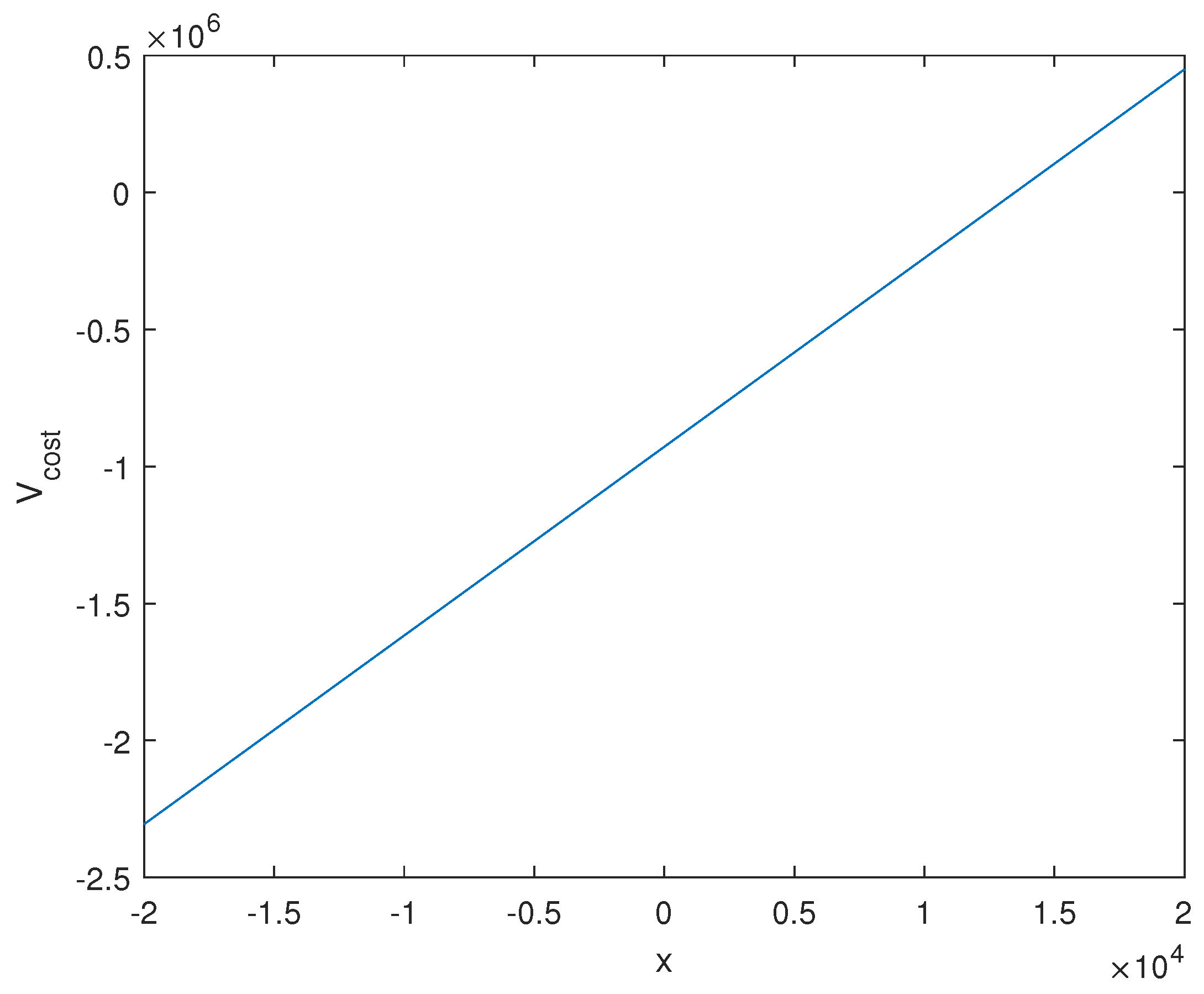
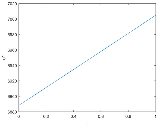
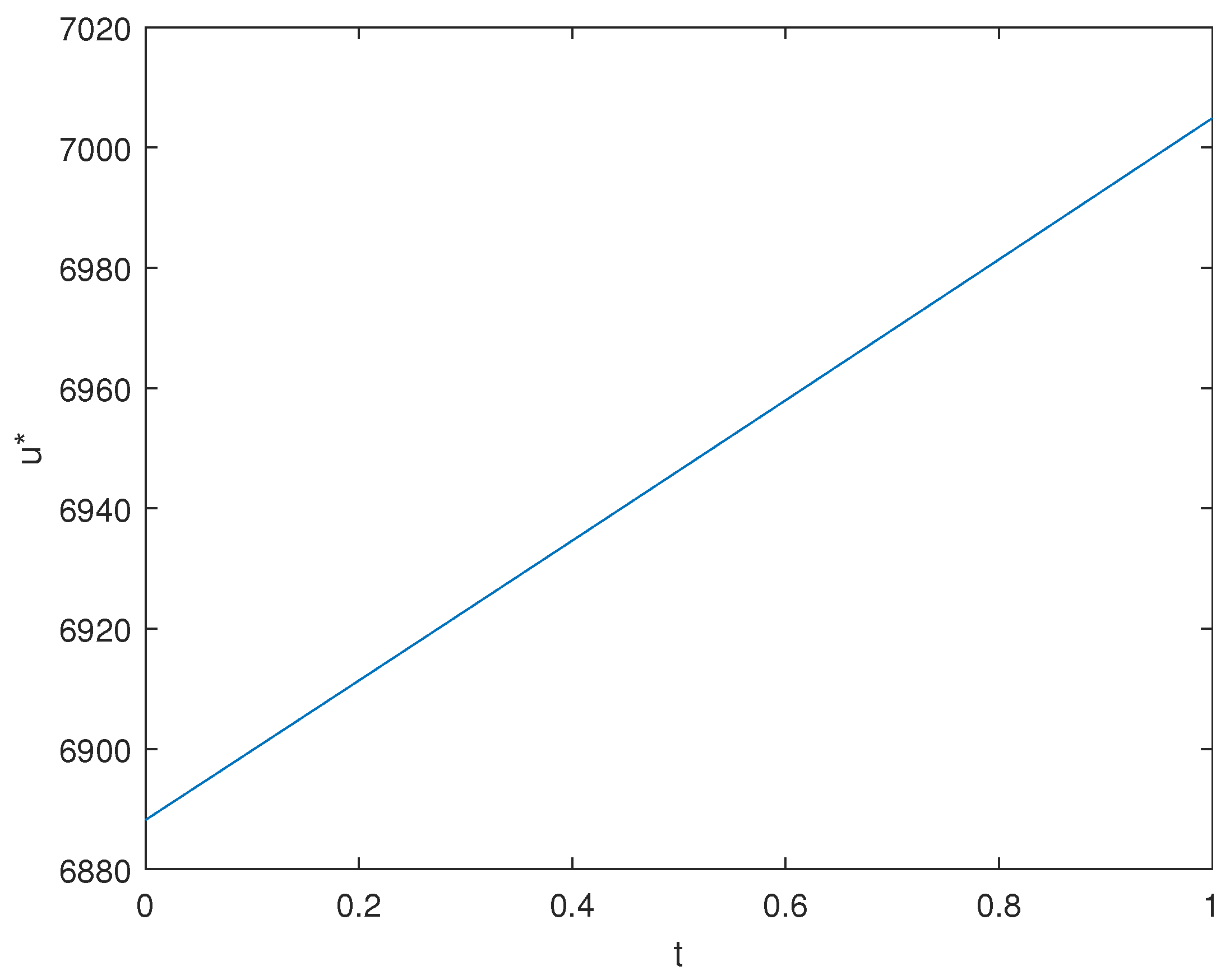
Furthermore, we also present the relationships between the minimum total cost, optimal emission reduction rate, and some parameters under the deterministic carbon allowance price model. As shown in Figure 9, the total cost increases with the expected emissions. Additionally, the closer the moment of verification is, the higher the optimal emission reduction rate becomes, as illustrated in Figure 10. Meanwhile, Figure 11 and Figure 12 demonstrate the impact of the emission reduction efficiency parameter m on these outcomes, which aligns with the findings in the stochastic model.
Figure 9.
Total cost under deterministic carbon allowance prices with x.
Figure 10.
Optimal emission reduction rate under deterministic carbon allowance prices with t.
Figure 11.
Total cost under deterministic carbon allowance prices with m.
Figure 12.
Optimal emission reduction rate under deterministic carbon allowance prices with m.
Based on a comprehensive analysis of the above discussions, the key findings and comparative insights are summarized as follows: For the stochastic carbon price model, the firm’s minimum total cost is positively correlated with its expected carbon emissions (Figure 1). The relationship between the carbon price and total cost, however, is dual-faceted: When initial expected emissions are low, the firm can profit from selling surplus allowances, so a higher carbon price leads to lower total costs. When initial expected emissions are high, the firm must buy additional allowances, so a higher carbon price leads to increased total costs. Additionally, the optimal emission reduction rate is influenced by both the carbon price and time (Figure 2): It increases with a rising carbon allowance price at any given time. It increases as the compliance deadline approaches, even if the carbon price remains constant. Furthermore, for the impact of key parameters under stochastic prices (Figure 3, Figure 4, Figure 5, Figure 6, Figure 7 and Figure 8), an increase in the emission reduction efficiency parameter (m) increases the total cost (Figure 3) and discourages abatement effort, thus decreasing the optimal emission reduction rate (Figure 4). Furthermore, due to the higher expected growth rate, the selling revenue is greater, thereby reducing the total cost (Figure 5). In response, the firm increases its optimal emission reduction rate to mitigate these higher future costs (Figure 6). The trends of the total cost and reduction rate relative to volatility align with those observed in (31) and (32). Ultimately, for validation in the context of deterministic carbon prices (Figure 9, Figure 10, Figure 11 and Figure 12), the core relationships hold in a deterministic price model, confirming the robustness of our findings. Specifically, the total cost increases with expected emissions (Figure 9). The emission reduction rate increases as the verification moment approaches (Figure 10). The influence of the emission reduction efficiency parameter (m) (Figure 11 and Figure 12) is consistent with the findings obtained with the stochastic model (Figure 3 and Figure 4).
5.3. Practical Implications
The above discussion provides a case for the practical application of the model, demonstrating how it transforms optimal emission reduction strategies into clear decision rules. This enables enterprises to determine optimal strategies directly from their specific parameters, eliminating the need for complex simulations. Further, the results explicitly reveal how key parameters directly influence optimal strategies, thereby significantly enhancing the model’s transparency, interpretability, and practical applicability. Based on the above analysis, we thus provide the following practical insights for carbon market participants (from corporate and government perspectives, respectively):
From an enterprise perspective, first of all, enterprises should establish a dedicated carbon asset management department responsible for continuously monitoring and updating key parameters, especially those related to carbon prices, to ensure strategies remain responsive to market dynamics. Parameters related to abatement efficiency should be reassessed following significant technological upgrades. Second, the results indicate that while total abatement costs rise with expected emission levels, their sensitivity to carbon prices exhibits a dual characteristic. This finding suggests that firms should dynamically adjust their strategies based on their marginal abatement costs and market price trends. For example: Low-emission industries may consider locking in trading positions during periods of rising carbon prices; High-emission industries should increase internal abatement investments to hedge against future cost risks. Furthermore, an increase in the abatement efficiency parameter (m-value) leads to higher total costs while suppressing the optimal abatement rate. Enterprises should therefore incorporate carbon price impacts into their evaluation criteria for technological retrofit projects. By comparing the marginal benefits of efficiency improvements against investment costs, firms can prioritize a transformation path from high m-value to low m-value technologies. As the expected growth rate of carbon prices increases, the future cost of purchasing quotas rises, incentivizing enterprises to enhance current abatement rates. Thus, carbon prices should be treated as a core parameter in investment assessments. When the expected market carbon price growth rate exceeds the marginal abatement cost, firms should prioritize emission reduction investments and establish a “carbon price–investment” linkage mechanism to ensure strategic alignment with market trends. Furthermore, from model output to cash flow management: The optimal strategies and directly translate into a forecasted cash flow profile for carbon-related activities. The term in Equation (2) represents the present value of a planned outflow for internal abatement investments, spread over time. The optimal determines an immediate cash outflow (if purchasing). Finally, the stochastic terminal term represents a hedged future cash flow exposure, converting an uncertain regulatory liability/asset into a planned present cost. By implementing the model, a company shifts from facing uncertain future carbon penalties to executing a sequenced financial plan, thereby improving cash flow predictability and budgeting accuracy.
From a government perspective, first, when designing industry-specific emission reduction standards or quota allocation schemes, the government should account for differences in marginal abatement costs across sectors. For industries with low abatement efficiency (high m-value), targeted subsidies or innovation incentives can be introduced to reduce m-value, thereby enhancing overall market efficiency. In determining free quota allocations and compliance cycle duration, policymakers must balance dual objectives: Excessive free quotas may undermine corporate abatement incentives and weaken carbon price signals; Excessively short compliance cycles could lead firms to prioritize short-term compliance over long-term low-carbon investments. Second, the government can mitigate systemic risks from market volatility by establishing price stabilization mechanisms. For instance, implementing a price floor to prevent carbon prices from falling too low and eroding abatement motivation; Setting a price ceiling to avoid excessive carbon prices escalating compliance costs for enterprises. Additionally, regulators should leverage volatility data to gauge market sentiment and dynamically adjust quota supply or release reserves accordingly. Such measures would enhance carbon market liquidity and resilience while ensuring stable progress toward emission reduction goals.
In summary, the numerical results in this section provides relatively complete practical insights for carbon market participants on how to apply this theoretical model to practice. Enterprises can use the described parameter calibration methods to estimate key variables and solve the model to derive optimal abatement pathways and cost-minimizing strategies over the full compliance cycle. For policymakers, the results also provide valuable references for refining mechanisms such as quota allocation and price regulation. Furthermore, the model explicitly identifies the risk-free interest rate r as a critical parameter determining the optimal strategy, particularly in the decision to purchase allowances upfront Equations (27) and (32). This establishes a direct channel through which macroeconomic and monetary policy can influence corporate carbon management. Future research could powerfully extend this work by incorporating endogenous economic policy scenarios. For instance, an expansionary monetary policy that lowers r would, ceteris paribus, increase the present value of future carbon costs, making early technological investments in abatement more attractive relative to purchasing allowances later. Conversely, a tightening cycle could have the opposite effect. This “domino effect” where policy affects r, which alters the optimal (, ) mix, thereby shifting demand for low-carbon technologies and ultimately impacting the global cost trajectory of the energy transition—represents a promising avenue for integrating stochastic carbon control models with dynamic macro-financial frameworks.
5.4. Model Generalizability to Other Carbon Markets
While our calibration uses data from China’s national carbon market, the model structure is general and can be adapted to other jurisdictions. The key to transferability lies in re-calibrating the following market-specific parameters:
For price dynamics (, ): In more mature markets like the EU ETS, the drift may reflect different macroeconomic and policy expectations, while volatility can be estimated from longer and more liquid price series. For policy parameters (T, ): Compliance periods (T) and free allocation rules () vary across systems. For example, the EU ETS operates in multi-year phases with declining caps, which can be modeled by adjusting over time. Besides, the emission reduction efficiency parameter (m) should be re-estimated using local MAC data, which can be derived from country-specific marginal abatement cost studies or technology databases. The risk-free rate (r) should reflect the local currency government bond yield. We provide a summary of adaptable parameters and suggested data sources for major carbon markets in Table 2 below.
Table 2.
Parameter adaptation guide for selected carbon markets.
This adaptability ensures that the model can serve as a versatile decision-support tool for multinational firms operating in multiple carbon markets or for policymakers designing new emissions trading systems.
6. Concluding Remarks
6.1. Main Findings and Contributions
This study develops a stochastic optimal control model for corporate carbon management that integrates internal abatement efforts with carbon market trading mechanisms. The model is solved under both deterministic and stochastic carbon price scenarios using a two-stage optimization procedure. The core theoretical contribution is the derivation of an explicit analytical solution to the HJB equation, achieved by leveraging the Linear–Quadratic structure of the problem. This transforms the optimal strategy into a clear decision rule. Empirically, the model is calibrated with actual data from China’s national carbon market, and numerical simulations vividly illustrate the influence of key parameters, such as carbon price, abatement efficiency, and interest rates, on the optimal emission reduction rate and total cost. The numerical results bridge theoretical modeling and practical application. For enterprises, the findings underscore the necessity of establishing a dynamic carbon asset management function. Key operational insights include: (i) total cost is positively correlated with expected emissions, but the sensitivity to carbon price is dual-faceted—firms with surplus allowances may benefit from rising prices, while those with a deficit face higher costs; (ii) the optimal abatement rate increases with both the carbon price and as the compliance deadline approaches. Firms should therefore continuously monitor key parameters and adjust their mix of internal abatement and market transactions accordingly. For policymakers, the model offers quantitative insights for market design. It highlights how factors like abatement efficiency (m), free quota allocation (), and compliance period (T) influence corporate behavior, informing the calibration of allocation rules and the potential design of price stabilization mechanisms (e.g., floors and ceilings) to ensure both environmental effectiveness and economic efficiency. Furthermore, while the analytical solution provides a clear decision rule, its practical implementation requires several prerequisites and faces operational challenges. First, enterprises need to establish a dedicated carbon asset management function capable of continuously monitoring and updating key parameters, particularly carbon price trends (, ) and firm-specific abatement efficiency (m). This may involve integrating real-time market data feeds and periodic reassessment of internal abatement technologies. Second, the model assumes that enterprises can accurately forecast their cumulative emissions () and dynamically adjust the abatement rate (). In practice, this requires robust emissions monitoring and reporting systems, as well as operational flexibility to adjust production or abatement technologies in response to control signals. Third, integrating the model into existing enterprise resource planning or environmental management systems may require software adaptation and staff training. The decision rule in the stochastic case can be embedded as a module that recommends daily or weekly abatement adjustments based on updated parameter inputs. Potential challenges include: parameter uncertainty, especially in volatile carbon markets; Lags in abatement technology deployment; Regulatory changes affecting quota allocation or penalty structures. Despite these challenges, the model offers a structured framework for carbon management that enhances strategic clarity and supports data-driven decision-making. Collectively, this work provides enterprises with a decision-support tool that combines theoretical rigor with actionable insights for navigating carbon markets and achieving compliance in a cost-optimal manner.
6.2. A Comparison with Numerical Methods
A pivotal advancement of this study is obtaining a closed-form analytical solution. Compared to the numerical approximation methods (e.g., finite difference, Monte Carlo simulation) commonly employed in prior literature, the analytical approach offers distinct advantages, as summarized in Table 3.
Table 3.
Comparison between analytical solution and numerical approximation approaches.
Consequently, the analytical solution elevates the model from a simulation tool to a prescriptive decision rule, significantly enhancing its practical utility for corporate decision-makers who require timely, interpretable, and robust guidance.
6.3. Limitations and Future Research Directions
This paper adopts a quadratic abatement cost function, i.e., . This assumption implies a linearly increasing marginal abatement cost (MAC), which endows the HJB equation with a quasilinear structure amenable to closed-form solution. From an empirical perspective, a quadratic function can provide a reasonable fit for cost data within moderate abatement ranges and aligns with the fundamental economic principle of increasing marginal costs. However, we acknowledge the limitations of this assumption. In practice, MAC curves may exhibit non-smooth characteristics or even discontinuities due to technological leaps, regulatory thresholds, or resource constraints. For instance, the adoption of carbon capture and storage (CCS) technology often involves a significant fixed cost, leading to a jump in the MAC curve once a certain emission reduction threshold is crossed. Similarly, sector-specific abatement options (e.g., fuel switching in power generation and process improvements in cement production) may create a piecewise MAC structure. Relaxing this assumption would likely preclude an explicit analytical solution, but we can prove the existence and uniqueness of a classical solution to the corresponding HJB equation (see prior work [20]) and the description of its solution needs to be characterized through numerical methods. Nevertheless, the quadratic form provides a tractable approximation that captures the increasing cost of deeper emission reductions, which is a common feature in many abatement scenarios. The model’s qualitative insights, such as the trade-off between internal abatement and market purchases, remain relevant even if the functional form is generalized, though the precise optimal rates would differ. Therefore, the model under the quadratic assumption establishes a clear benchmark and delivers intuitive economic insights. Furthermore, it provides a reference point for the construction and calibration of more complex models.
The current study focuses on deriving an analytical decision rule and demonstrating its numerical properties. A full empirical backtest against actual firm-level abatement decisions or aggregate market outcomes is beyond its scope, primarily due to the lack of publicly available, high-frequency data on firm-specific abatement actions and internal carbon trading strategies. However, we outline potential approaches for future empirical validation and back testing. First, for the aggregate market test, we can compare model-predicted aggregate allowance demand with actual auction results or secondary market net positions in markets with transparent data. Second, for the sectoral calibration, we can use sector-average abatement cost curves and observed emission trends to see if the model’s predicted abatement rates align with historical sectoral emission reductions. Last, for the controlled case studies, we can collaborate with participating firms to implement the model in real time and compare its prescriptions with actual management decisions, adjusting for unmodeled constraints. We acknowledge that such validation is an essential next step to confirm the model’s predictive power and encourage future research in this direction.
In summary, this study provides a solid framework, several limitations point to fruitful directions for future research: The quadratic abatement cost and geometric Brownian motion price dynamics are useful approximations but may not capture all real-world complexities. Future work could explore alternative cost structures (e.g., piecewise convex, incorporating learning-by-doing) and price processes (e.g., mean-reverting with jumps). In addition, the model considers an isolated firm in a single compliance period. Extensions could include multi-period dynamics with banking/borrowing of allowances, strategic interactions in oligopolistic markets, or supply chain coordination mechanisms. Furthermore, the carbon price is exogenous. A promising direction is to embed the firm-level model into a general equilibrium or agent-based framework to study the endogenous feedback between aggregate abatement actions and allowance prices. A full empirical backtest against actual firm-level decisions remains an open challenge due to data limitations. Future research could involve collaborations with industry to access proprietary data or utilize sectoral emission trends for indirect validation. The model minimizes compliance costs. Integrating carbon constraints into a holistic corporate planning model that simultaneously considers production, finance, and reputational goals would be a valuable step towards more comprehensive decision-support systems.
Author Contributions
Conceptualization, W.H.; methodology, W.H.; software, D.S.; validation, D.S.; formal analysis, D.S.; investigation, D.S.; resources, W.H.; data curation, W.H.; writing—original draft preparation, D.S.; writing—review and editing, W.H.; visualization, D.S.; supervision, W.H.; project administration, W.H.; funding acquisition, W.H. All authors have read and agreed to the published version of the manuscript.
Funding
This work is supported by the National Natural Science Foundation of China (No. 12401618).
Data Availability Statement
The original contributions presented in this study are included in the article; further inquiries can be directed to the corresponding author.
Conflicts of Interest
The authors declare no conflicts of interest.
Appendix A
Theorem A1.
For all , we have
Proof.
On the one hand, for any , , we have
Since u is arbitrary, we have
Then, according to the arbitrariness of , we can obtain
On the other hand, first assume that . For all , there exists , such that
Since
then
Since is arbitrary, we have
If , then for all , there exists , such that
Similarly, we shall have
Letting , we shall have the same result. □
References
- Dales, J.H. Pollution, Property and Prices; University of Toronto Press: Toronto, ON, Canada, 1968. [Google Scholar]
- Montgomer, W.D. Markets in licenses and efficient pollution control programs. J. Econ. Theory 1972, 5, 395–418. [Google Scholar] [CrossRef] [Scilit]
- Benz, E.; Truck, S. Modeling the price dynamics of CO2 emission allowances. Energy Econ. 2009, 31, 4–15. [Google Scholar] [CrossRef] [Scilit]
- Koop, G.; Tole, L. Forecasting the European carbon market. J. R. Stat. Soc. A Stat. 2013, 76, 723–741. [Google Scholar] [CrossRef] [Scilit]
- Seifert, J.; Uhrig-Homburg, M.; Wagner, M. Dynamic behavior of CO2 spot prices. J. Environ. Econ. Manag. 2008, 56, 180–194. [Google Scholar] [CrossRef] [Scilit]
- Carmona, R.; Fehr, M.; Hinz, J. Optimal stochastic control and carbon price formation. SIAM J. Control Optim. 2009, 48, 2168–2190. [Google Scholar] [CrossRef] [Scilit]
- Carmona, R.; Fehr, M.; Hinz, J.; Porchet, A. Market design for emission trading schemes. SIAM Rev. 2010, 52, 403–452. [Google Scholar] [CrossRef] [Scilit]
- Hinz, J.; Novikov, A. On fair pricing of emission-related derivatives. Bernoulli 2010, 16, 1240–1261. [Google Scholar] [CrossRef] [Scilit]
- Carmona, R.; Delarue, F.; Espinosa, G.E.; Touzi, N. Singular forward-backward stochastic differential equations and emissions derivatives. Ann. Appl. Probab. 2013, 23, 1086–1128. [Google Scholar] [CrossRef] [Scilit]
- Carmona, R.; Hinz, J. Risk-neutral models for emission allowance prices and option valuation. Manag. Sci. 2011, 57, 1453–1468. [Google Scholar] [CrossRef] [Scilit]
- Cetin, U.; Verschuere, M. Pricing and hedging in carbon emissions markets. Int. J. Theor. Appl. Fin. 2009, 12, 949–967. [Google Scholar] [CrossRef] [Scilit]
- Zagheni, E.; Billari, F.C. A cost valuation model based on a stochastic representation of the IPAT equation. Popul. Environ. 2007, 29, 68–82. [Google Scholar] [CrossRef] [Scilit]
- Yang, X.; Liang, J. Minimization of the nation cost due to carbon emission. Syst. Eng. Theory Pract. 2014, 34, 640–647. [Google Scholar]
- Merton, R.C. Optimum consumption and portfolio rules in a continuous-time model. J. Econ. Theory 1971, 3, 373–413. [Google Scholar] [CrossRef] [Scilit]
- Merton, R.C. Lifetime portfolio selection under uncertainty: The continuous-time case. Rev. Econ. Stat. 1969, 51, 247–257. [Google Scholar] [CrossRef] [Scilit]
- Yang, X.; Liang, J.; Hu, B. Minimization of carbon abatement cost: Modeling, analysis and simulation. Discret. Cont. Dyn-B. 2017, 22, 2939–2969. [Google Scholar] [CrossRef] [Scilit]
- Guo, H.; Liang, J. An optimal control model for reducing and trading of carbon emissions. Phys. A 2016, 446, 11–21. [Google Scholar] [CrossRef] [Scilit]
- Guo, H.; Liang, J. An optimal control model of carbon reduction and trading. Math. Control Relat. Fields 2016, 6, 535–550. [Google Scholar] [CrossRef] [Scilit]
- Liang, J.; Huang, W. Optimal control model of an enterprise for single and inheriting periods of carbon emission reduction. Math. Financ. Econ. 2022, 16, 89–123. [Google Scholar] [CrossRef] [Scilit]
- Huang, W. Optimal stochastic control for carbon emission with allowances trading. Appl. Anal. 2025, 104, 2250–2270. [Google Scholar] [CrossRef] [Scilit]
- Huang, W.; Liang, J.; Dong, Y. Optimal stochastic control problem for a carbon emission reduction process. SIAM J. Appl. Math. 2023, 83, 1272–1295. [Google Scholar] [CrossRef] [Scilit]
- Aid, R.; Biagini, S. Optimal dynamic regulation of carbon emissions market. Math. Financ. 2023, 33, 80–115. [Google Scholar] [CrossRef] [Scilit]
- Wang, X.; Zhang, T.; Yuan, S. Dynamical analysis and near-optimal control strategy of a stochastic carbon emissions model. Chaos 2025, 35, 103103. [Google Scholar] [CrossRef] [Scilit] [PubMed]
- Kalman, R. Contributions to the theory of optimal control. Bol. Soc. Mat. Mexicana. 1960, 5, 102–119. [Google Scholar]
- Bellman, R. Dynamic Programming; Princeton University Press: Princeton, NJ, USA, 1957. [Google Scholar]
- Gollier, C. The cost efficiency carbon pricing puzzle. J. Environ. Econ. Manag. 2024, 128, 103062. [Google Scholar] [CrossRef] [Scilit]
- Pham, H. Continuous-Time Stochastic Control and Optimization with Financial Applications; Springer: Berlin/Heidelberg, Germany, 2009. [Google Scholar]
- Fleming, W.; Soner, H. Controlled Markov Processes and Viscosity Solutions; Springer: New York, NY, USA, 2006. [Google Scholar]
- Yong, J.; Zhou, X. Stochastic Controls: Hamiltonian Systems and HJB Equations; Springer: New York, NY, USA, 1999. [Google Scholar]
- Zheng, Y. Carbon Option Product Design and Pricing Based on Carbon Emission Quota. Master’s Thesis, Northwest Normal University, Lanzhou, China, 2024. [Google Scholar]

Disclaimer/Publisher’s Note: The statements, opinions and data contained in all publications are solely those of the individual author(s) and contributor(s) and not of MDPI and/or the editor(s). MDPI and/or the editor(s) disclaim responsibility for any injury to people or property resulting from any ideas, methods, instructions or products referred to in the content. |
© 2025 by the authors. Licensee MDPI, Basel, Switzerland. This article is an open access article distributed under the terms and conditions of the Creative Commons Attribution (CC BY) license.