Two-Dimensional Probability Models for the Weighted Discretized Fréchet–Weibull Random Variable with Min–Max Operators: Mathematical Theory and Statistical Goodness-of-Fit Analysis

Abstract

This study introduces two bivariate extensions of the recently proposed weighted discretized Fréchet–Weibull distribution, termed as bivariate weighted discretized Fréchet–Weibull (BWDFW) distributions. These models are specifically designed for analyzing two-dimensional discrete datasets and are developed using two distinct structural approaches: the minimum operator (BWDFW-I) and the maximum operator (BWDFW-II). A rigorous mathematical formulation is presented, encompassing the joint cumulative distribution function, joint probability mass function, and joint (reversed) hazard rate function. The dependence structure of the models is investigated, demonstrating their capability to capture positive quadrant dependence. Additionally, key statistical measures, including covariance, Pearson’s correlation coefficient, Spearman’s rho, and Kendall’s tau, are derived using the joint probability-generating function. For robust statistical inferences, the parameters of the proposed models are estimated via the maximum likelihood estimation method, with extensive simulation studies conducted to assess the efficiency and accuracy of the estimators. The practical applicability of the BWDFW distributions is demonstrated through their implementation in two real-world datasets: one from the aviation sector and the other from the security and safety domain. Comparative analyses against four existing discrete bivariate Weibull extensions reveal the superior performance of the BWDFW models, with BWDFW-I (minimum operator based) exhibiting greater flexibility and predictive accuracy than BWDFW-II (maximum operator based). These findings underscore the potential of the BWDFW models as effective tools for modeling and analyzing bivariate discrete data in diverse applied contexts.

1. Introduction

The Fréchet and Weibull distributions hold a prominent place in research because of their versatility and wide-ranging applications. These continuous probability models are renowned for their ability to encapsulate the characteristics of various other continuous distributions, making them highly adaptable to diverse scenarios. Both distributions are extensively studied as extreme value models, particularly in reliability and survival analysis, where they effectively model critical phenomena. Their applicability spans a broad spectrum of disciplines, including physical sciences, chemistry, environmental studies, medicine, and engineering, where experimental data often exhibit behaviors that align with their properties. This widespread utility underscores their importance as foundational tools in statistical modeling and analysis.

In recent years, numerous generalized distributions have been developed and employed to model a wide range of phenomena. A key characteristic of these generalized distributions is their inclusion of additional parameters, enhancing their flexibility and applicability. Teamah et al. [1] introduced the relatively new Fréchet–Weibull (FW) distribution, which is derived using the T-X method for generating distribution families, as proposed by Alzaatreh et al. [2]. The authors explored the statistical properties of the FW distribution and demonstrated its practical utility by applying it to earthquake datasets. This distribution offers a more adaptable framework for modeling experimental data, with applications consistently demonstrating its superiority in fitting data compared to other extensions of the Weibull distribution.

Although continuous probability distributions play significant roles in various fields, there are numerous practical scenarios where discrete probability distributions are indispensable. In certain cases, measuring the life length of a machine on a continuous scale is either impractical or impossible. Examples include the on–off switching cycles of machines or the lifespan of photocopier bulbs. To address such needs, Das and Das [3] introduced a four-parameter discrete distribution, known as the discretized Fréchet–Weibull (DFW) distribution, derived as a discrete counterpart of the continuous Fréchet–Weibull distribution. This novel discrete distribution was constructed using the survival function approach to discretization, endowing it with a range of flexible properties. The DFW distribution is capable of modeling data with both positive and negative skewness. Additionally, its hazard rate function (HRF) exhibits diverse shapes, including increasing, decreasing, and upside-down bathtub forms, behaviors not commonly observed in many count data distributions. The probability mass function (PMF) of a random variable (Y), following the DFW distribution with shape parameters $\alpha$ and k, and scale parameters $\beta$ and m, is expressed as follows:

$$P_{DFW}[Y=y]=exp\left\{-{\beta }^{\alpha }{\left({\displaystyle \frac{m}{y+1}}\right)}^{\alpha k}\right\}-exp\left\{-{\beta }^{\alpha }{\left({\displaystyle \frac{m}{y}}\right)}^{\alpha k}\right\},$$

(1)

where $y\in {\mathbf{Z}}_{+}$, and the parameters $(\alpha ,\beta ,m,k)>0$. Let $\xi$ denote the parameter vector of the DFW distribution, defined as $\xi =(\alpha ,\beta ,m,k)$, where $\xi \in {\mathbb{R}}_{+}\times {\mathbb{R}}_{+}\times {\mathbb{R}}_{+}\times {\mathbb{R}}_{+}$. This construction highlights the versatility of the DFW distribution in modeling discrete data arising from real-world applications.

In a subsequent development, Das and Das [4] introduced a novel discrete distribution termed as the weighted discretized Fréchet–Weibull (WDFW) distribution. This distribution builds upon the CDF of the discrete Weibull (DW) distribution to define the weight function as follows:

$$w\left(y\right)=1-exp\left\{-{\left({\displaystyle \frac{y+1}{m}}\right)}^k\right\},y\in {\mathbf{Z}}_{+},$$

where $(m,k)>0$. The choice of this CDF as the weight function is motivated by its non-negativity and its asymptotic behavior, $w\left(y\right)\to 1$ as $k\to \infty$. This weight function plays a crucial role in constructing the WDFW model by modifying the probabilities of the parent distribution to capture complex data behaviors. The PMF of $Y\sim \mathrm{WDFWD}(\alpha ,\beta ,m,k)$ is given as follows:

$$P_{WDFW}[Y=y;\xi ]={\displaystyle \frac{q(y;\xi )}{{\sum }_{s=0}^{\infty }q(s;\xi )}}={\displaystyle \frac{q(y;\xi )}{Q(y;\xi )}}.$$

(2)

The corresponding CDF and survival function (SF) are expressed as follows:

$$\begin{array}{ccc}\hfill F_{WDFW}(y;\xi )& =& {\displaystyle \frac{{\sum }_{s=0}^{y}q(s;\xi )}{Q(y;\xi )}}={\displaystyle \frac{V(y;\xi )}{Q(y;\xi )}},\hfill \end{array}$$

(3)

$$\begin{array}{ccc}\hfill S_{WDFW}(y;\xi )& =& 1-F_{WDFW}(y;\xi )+P_{WDFW}[Y=y;\xi ].\hfill \end{array}$$

(4)

where $q(y;\xi )$ and $Q(y;\xi )$ are defined as follows:

$$\begin{array}{ccc}\hfill q(y;\xi )& =& w\left(y\right)·P[Y=y],\hfill \\ \hfill Q(y;\xi )& =& \sum _{s=0}^{\infty }q(s;\xi ),\hfill \end{array}$$

where $q(y;\xi )$ is computed using the weight function ($w\left(y\right)$) and the PMF of the discretized Fréchet–Weibull distribution. Although $Q(y;\xi )$ lacks a closed-form expression, it is finite and can be evaluated numerically. The theory of weighted distributions provides a cohesive framework for addressing model specification and interpreting diverse datasets. Weighted distributions are commonly encountered in fields such as survival analysis, intervention studies, ecology, and biomedicine. A notable aspect of the proposed WDFW distribution is that the introduction of the weight function does not increase the number of parameters relative to the parent distribution, maintaining parsimony. Furthermore, this distribution exhibits diverse hazard rate functions, including increasing, decreasing, and bathtub-shaped behaviors, which are rarely observed in count data models. With support on the set of positive integers, the WDFW distribution proves to be a versatile tool for modeling overdispersed count data, offering a promising alternative for real-world applications requiring such flexibility.

Research on bivariate distributions has been a focal point for statisticians for decades because of their relevance in modeling real-life phenomena involving two dimensions. In statistics, bivariate probability distributions are essential for describing scenarios where two interdependent variables are present. Univariate distributions are insufficient for such data, emphasizing the necessity of bivariate models. These models find applications in diverse fields, such as engineering, reliability, meteorology, drought analysis, sports (e.g., goals scored by two competing teams), insurance claims for different causes, symptom types in patients with the same disease, academic performance in two subjects, and many other areas.

Bivariate data naturally occur in many practical settings, driving the development of specialized models to analyze such datasets. These models play a critical role in understanding two-dimensional data structures that arise in a variety of disciplines. The literature contains numerous bivariate extensions of both continuous and discrete univariate distributions. Comprehensive overviews on bivariate distributions are available in the works of Johnson et al. [5] and Balakrishnan and Lai [6], which focus on discrete and continuous distributions, respectively. For continuous bivariate distributions, significant contributions include studies by Kundu and Gupta [7], Sarhan et al. [8], El-Sherpieny [9], Wagner and Artur [10], Balakrishnan and Shiji [11], and El-Gohary et al. [12]. Recent advancements include the bivariate Weibull distribution by Hiba [13], the bivariate exponentiated extended Weibull distribution by Rasool and Akbar [14], the bivariate Gumbel-G family of distributions, and the bivariate odd Weibull-G family of distributions introduced by Eliwa and El-Morshedy [15].

Detailed surveys on discrete bivariate distributions are provided by Kocherlakota and Kocherlakota [16] and Johnson et al. [5]. Further contributions can be found in the works of Basu and Dhar [17], Kumar [18], Kemp [19], Lee and Cha [20], and Nekoukhou and Kundu [21]. Recent developments in discrete bivariate distributions encompass a range of innovative models: the bivariate discrete exponentiated Weibull distribution by El-Morshedy et al. [22] and the bivariate discrete Nadarajah and Haghighi distribution discussed by Ali et al. [23]. Other notable advancements include the bivariate discrete Weibull distribution proposed by Kundu and Nekoukhou [24] and the bivariate discrete modified Weibull distribution developed by Shibu and Beegum [25].

This paper introduces a new flexible discrete bivariate distribution called the BWDFW distribution, designed for application in various data fields. The proposed discrete bivariate model is constructed using three independent random variables that follow the WDFW distribution. The development of the BWDFW distribution is based on two techniques: the minimum operator and the maximum operator, as outlined by Lee and Cha [20]. The model derived using the minimum operator is denoted as BWDFW-I, while the one based on the maximum operator is referred to as BWDFW-II. The motivation for introducing the BWDFW distribution stems from multiple considerations:

1.

The proposed distribution is a bivariate extension of the WDFW distribution, offering a robust framework for modeling dispersion phenomena and addressing complex real-life discrete datasets.

2.

The joint PMF of the proposed model exhibits remarkable flexibility, allowing for diverse shapes influenced by parameter values. This adaptability makes it suitable for evaluating asymmetric data under various kurtosis structures.

3.

The joint HRF and its marginals of the proposed distribution are WDFW distributions, enabling the analysis of various hazard rate functions, such as increasing, decreasing, and bathtub-shaped rates, in discrete settings. This capability supports the comprehensive modeling of diverse data types.

4.

The BWDFW distribution possesses positive quadrant dependence, a critical property for modeling interdependencies in bivariate data. This characteristic enhances its relevance in applications requiring the joint modeling of correlated phenomena.

5.

The straightforward generation mechanism of the BWDFW distribution facilitates simulation studies, while its versatility makes it applicable to a wide range of fields, including engineering, reliability, and social sciences.

This paper is structured as follows: Section 2 explores the two primary methods for generating discrete bivariate distributions: the minimum operator and the maximum operator. Section 3 introduces the BWDFW distributions, derived using both operators, leading to the BWDFW-I and BWDFW-II models. The examination of positive quadrant dependence is presented in Section 4. Section 5 derives various moments, using the joint probability-generating function. The maximum likelihood estimation method for the model’s unknown parameters is discussed in Section 6, with simulation results presented in Section 7. In Section 8, the application of the BWDFW-I and BWDFW-II models to two bivariate count datasets illustrates their superiority over four alternative bivariate distributions. Finally, Section 9 summarizes the key findings, and Section 10 outlines potential future research directions.

2. Construction of a Bivariate Distribution

Consider three independent discrete random variables, $U_1,U_2,$ and $U_3$, with probability mass functions $f_1\left(y\right),f_2\left(y\right),$ and $f_3\left(y\right)$, respectively. Their corresponding cumulative distribution functions and survival functions are denoted by $F_1\left(y\right),F_2\left(y\right),F_3\left(y\right)$ and $S_1\left(y\right),S_2\left(y\right),S_3\left(y\right)$, respectively. The construction of a bivariate distribution can be achieved using the minimum and maximum operators. Specifically, the minimum operator utilizes the SF of the baseline distribution, while the maximum operator employs the CDF.

2.1. The Minimum Operator

Now consider the following six mutually exclusive cases that encompass all the possible outcomes regarding $U_1,U_2,$ and $U_3$:

$$\begin{array}{ccc}\hfill \mathrm{Case}1:\{U_2<U_1\le U_3\},& \mathrm{Case}2:\{U_2<U_3<U_1\},& \mathrm{Case}3:\{U_1<U_2\le U_3\},\hfill \\ \hfill \mathrm{Case}4:\{U_1<U_3<U_2\},& \mathrm{Case}5:\{U_3\le U_1,U_2\},& \mathrm{Case}6:\{U_2=U_1<U_3\}.\hfill \end{array}$$

Theorem 1. 

Let $U_1,U_2,U_3$ be three independent baseline random variables. If $Y_1=min\{U_1,U_3\}$ and $Y_2=min\{U_2,U_3\}$ then the joint probability mass function is given by

$$\begin{array}{c}\hfill f(y_1,y_2)=\left\{\begin{array}{cc}{f}_2\left(y_2\right)\left\{f_1\left(y_1\right)S_3(y_1-1)+f_3\left(y_1\right)S_1\left(y_1\right)\right\}\hfill & ;y_1>y_2,\hfill \\ f_1\left(y_1\right)\left\{f_2\left(y_2\right)S_3(y_2-1)+f_3\left(y_2\right)S_2\left(y_2\right)\right\}\hfill & ;y_1<y_2,\hfill \\ f_3\left(y\right)S_2(y-1)S_1(y-1)+f_1\left(y\right)f_2\left(y\right)S_3\left(y\right)\hfill & ;y_1=y_2=y,\hfill \end{array}\right.\end{array}$$

(5)

where $f_i(.)$ and $S_i(.)$ are the PMF and SF of the baseline random variable.

Proof. 

To obtain the joint PMF of $(Y_1,Y_2)$, we need to consider the six mutually exclusive subcases, as mentioned in Section 2.1.

Case 1: 

$y_1>y_2$

Here, we focus on the relation $Y_1=min\{U_1,U_3\}$. The value of $Y_1$ can be determined by $U_1$ or solely by $U_3$. Thus, we follow subcases 1 and 2. Also, these two cases are mutually exclusive. First, when the value of $Y_1$ is determined by $U_1$, we have subcase 1, therefore

$$\begin{array}{ccc}\hfill P[Y_1=y_1,Y_2=y_2]& =& P(U_1=y_1,U_2=y_2,U_3\ge y_1)\hfill \\ & =& f_1\left(y_1\right)f_2\left(y_2\right)S_3(y_1-1).\hfill \end{array}$$

(6)

Second, when the value of $Y_1$ is determined by $U_3$, we have subcase 2, therefore

$$\begin{array}{ccc}\hfill P[Y_1=y_1,Y_2=y_2]& =& P(U_3=y_1,U_2=y_2,U_1\ge y_1)\hfill \\ & =& f_3\left(y_1\right)f_2\left(y_2\right)S_1\left(y_1\right).\hfill \end{array}$$

(7)

Because subcases 1 and 2 are mutually exclusive, we obtain the desirable result by combining Equations (6) and (7).

Case 2: 

$y_2>y_1$

In this case, we focus on the relation $Y_2=min\{U_2,U_3\}$. The value of $Y_2$ can be determined by $U_2$ or solely by $U_3$. Here, we follow subcases 3 and 4. Proceeding similarly as in case 1, we obtain

$$\begin{array}{ccc}\hfill P[Y_1=y_1,Y_2=y_2]& =& P(U_2=y_2,U_1=y_1,U_3\ge y_2)+P(U_3=y_2,U_1=y_1,U_2>y_2)\hfill \\ & =& f_2\left(y_2\right)f_1\left(y_1\right)S_3(y_2-1)+f_3\left(y_2\right)f_1\left(y_1\right)S_2\left(y_2\right).\hfill \end{array}$$

(8)

Case 3: 

$y_1=y_2=y$

In this case, the values of $Y_1$ and $Y_2$ can be determined by $U_3$ or solely by $(U_1,U_2)$. Here, we follow subcases 5 and 6, such that

$$\begin{array}{ccc}\hfill P[Y_1=y_1,Y_2=y_2]& =& P(U_3=y,U_2\ge y,U_1\ge y)+P(U_1=y,U_2=y,U_3>y)\hfill \\ & =& f_3\left(y\right)S_2(y-1)S_1(y-1)+f_1\left(y\right)f_2\left(y\right)S_3\left(y\right).\hfill \end{array}$$

(9)

Hence, the result. □

The concept of the minimum operator has several applications in statistics. For example, in lifetime modeling, an organism may die because of one of two distinct causes: Cause I or Cause II. Denote the times to death of Organisms 1 and 2 from Cause I by $U_1$ and $U_2$, respectively. Assume that Cause II represents a shared fatal environmental factor, causing both organisms to die simultaneously while exposed to the same environment. In such a scenario, the random variable $U_3$ is typically employed to represent the time to death resulting from Cause II. The competing risk models ($Y_1=min\{U_1,U_3\}$ and $Y_2=min\{U_2,U_3\}$) then define the lifespans of the organisms.

2.2. The Maximum Operator

The following six mutually exclusive cases encompass all the possible outcomes regarding $U_1,U_2,$ and $U_3$:

$$\begin{array}{ccc}\hfill \mathrm{Subcase}1:\{U_3\le U_2<U_1\},& \mathrm{Subcase}2:\{U_2<U_3<U_1\},& \mathrm{Subcase}3:\{U_1<U_3<U_2\},\hfill \\ \hfill \mathrm{Subcase}4:\{U_3\le U_1<U_2\},& \mathrm{Subcase}5:\{U_1,U_2\le U_3\},& \mathrm{Subcase}6:\{U_3<U_1=U_2\}.\hfill \end{array}$$

Theorem 2. 

For $U_1,U_2,U_3$ as three independent baseline random variables, if $Y_1=max\{U_1,U_3\}$ and $Y_2=max\{U_2,U_3\}$ then the joint probability mass function is given by

$$\begin{array}{c}\hfill f(y_1,y_2)=\left\{\begin{array}{cc}{f}_1\left(y_1\right)\left\{f_2\left(y_2\right)F_3\left(y_2\right)+f_3\left(y_2\right)F_2(y_2-1)\right\},\hfill & y_1>y_2,\hfill \\ f_2\left(y_2\right)\left\{f_1\left(y_1\right)F_3\left(y_1\right)+f_3\left(y_1\right)F_1(y_1-1)\right\},\hfill & y_1<y_2,\hfill \\ f_3\left(y\right)F_2\left(y\right)F_1\left(y\right)+f_1\left(y\right)f_2\left(y\right)F_3(y-1),\hfill & y_1=y_2=y,\hfill \end{array}\right.\end{array}$$

(10)

where $f_i(.)$ and $F_i(.)$ represent the PMF and CDF of the baseline random variable, respectively.

Proof. 

The joint probability mass function of $(Y_1,Y_2)$ is obtained by analyzing the six mutually exclusive subcases outlined in Section 2.2.

Case 1: 

$y_1>y_2$

The relationship $Y_1=max\{U_1,U_3\}$ is considered. The probability $P[Y_1=y_1,Y_2=y_2]$ depends on subcases 1 and 2:

$$\begin{array}{ccc}\hfill P[Y_1=y_1,Y_2=y_2]& =& P(U_1=y_1,U_2=y_2,U_3\le y_2)+P(U_1=y_1,U_3=y_2,U_2\le y_2)\hfill \\ & =& f_1\left(y_1\right)f_2\left(y_2\right)F_3\left(y_2\right)+f_1\left(y_1\right)f_3\left(y_2\right)F_2(y_2-1).\hfill \end{array}$$

(11)

Case 2: 

$y_2>y_1$

This case follows subcases 3 and 4. Using a similar approach as that in Case 1:

$$\begin{array}{ccc}\hfill P[Y_1=y_1,Y_2=y_2]& =& P(U_1=y_1,U_2=y_2,U_3\le y_1)+P(U_3=y_1,U_2=y_2,U_1<y_1)\hfill \\ & =& f_1\left(y_1\right)f_2\left(y_2\right)F_3\left(y_1\right)+f_3\left(y_1\right)f_2\left(y_2\right)F_1(y_1-1).\hfill \end{array}$$

(12)

Case 3: 

$y_1=y_2=y$

Subcases 5 and 6 are relevant here, leading to

$$\begin{array}{ccc}\hfill P[Y_1=y_1,Y_2=y_2]& =& P(U_3=y,U_1\le y,U_2\le y)+P(U_1=y,U_2=y,U_3<y)\hfill \\ & =& f_3\left(y\right)F_1\left(y\right)F_2\left(y\right)+f_1\left(y\right)f_2\left(y\right)F_3(y-1).\hfill \end{array}$$

(13)

This completes the proof. □

The maximal-operator-based construct can have meaningful statistical applications. For example, consider a scenario where an organism dies if its stress level exceeds a certain threshold. The stress levels $U_1$ and $U_2$ represent the separate, independent stresses experienced by Organisms 1 and 2. Additionally, both organisms are subjected to a common stress level ($U_3$). Then, $Y_1=max\{U_1,U_3\}$ and $Y_2=max\{U_2,U_3\}$ describe the dependent stress levels of the two organisms. The joint distribution of $(Y_1,Y_2)$ models the dependent joint life distribution of these organisms.

3. The Bivariate Weighted Discretized Fréchet–Weibull Distribution

3.1. The BWDFW Model Constructed Using the Minimum Operator

Suppose $U_1\sim \mathrm{WDFW}$$(\alpha ,{\beta }_1,m,k)$, $U_2\sim \mathrm{WDFW}(\alpha ,{\beta }_2,m,k)$, and $U_3\sim \mathrm{WDFW}$$(\alpha ,{\beta }_3,m,k)$, and these random variables are independently distributed. Define $Y_1=min\{U_1,U_3\}$ and $Y_2=min\{U_2,U_3\}$. Then, the bivariate vector $\mathbf{Y}=(Y_1,Y_2)$ follows a BWDFW distribution with the parameter vector $\Omega ={(\alpha ,{\beta }_1,{\beta }_2,{\beta }_3,m,k)}^{\top }$. This bivariate discrete distribution is denoted by $\mathrm{BWDFW}(\alpha ,{\beta }_1,{\beta }_2,{\beta }_3,m,k)$. The distribution BWDFW constructed using the minimum operator is referred to as the BWDFW-I model. The joint PMF of $(Y_1,Y_2)$ is expressed as

$$\begin{array}{ccc}\hfill f_{Y_1,Y_2}(y_1,y_2;\Omega )& =& P[Y_1=y_1,Y_2=y_2;\Omega ]\hfill \\ & =& \left\{\begin{array}{cc}{f}_1(y_1,y_2;\Omega ),\hfill & y_1>y_2,\hfill \\ f_2(y_1,y_2;\Omega ),\hfill & y_1<y_2,\hfill \\ f_3(y;\Omega ),\hfill & y_1=y_2=y,\hfill \end{array}\right.\hfill \end{array}$$

(14)

where the terms are defined as

$$\begin{array}{ccc}\hfill f_1(y_1,y_2;\Omega )& =& f_2\left(y_2\right)\left\{f_1\left(y_1\right)S_3(y_1-1)+f_3\left(y_1\right)S_1\left(y_1\right)\right\},\hfill \\ \hfill f_2(y_1,y_2;\Omega )& =& f_1\left(y_1\right)\left\{f_2\left(y_2\right)S_3(y_2-1)+f_3\left(y_2\right)S_2\left(y_2\right)\right\},\hfill \\ \hfill f_3(y;\Omega )& =& f_3\left(y\right)S_2(y-1)S_1(y-1)+f_1\left(y\right)f_2\left(y\right)S_3\left(y\right),\hfill \end{array}$$

where $f_i(·)$ and $S_i(·)$ represent the PMF and SF of $U_i\sim \mathrm{WDFW}(\alpha ,{\beta }_i,m,k)$.

3.1.1. The Joint SF of the BWDFW-I Model

The joint SF of $(Y_1,Y_2)$ is given by

$$\begin{array}{ccc}\hfill S_{Y_1,Y_2}(y_1,y_2;\Omega )& =& P[Y_1>y_1,Y_2>y_2;\Omega ]\hfill \\ & =& \left\{\begin{array}{cc}{S}_1(y_1,y_2;\Omega ),\hfill & y_1>y_2,\hfill \\ S_2(y_1,y_2;\Omega ),\hfill & y_2>y_1,\hfill \\ S_3(y;\Omega ),\hfill & y_1=y_2=y,\hfill \end{array}\right.\hfill \end{array}$$

(15)

where the terms are defined as follows:

$$\begin{array}{ccc}\hfill S_1(y_1,y_2;\Omega )& =& S_1\left(y_1\right)S_2\left(y_2\right)S_3\left(y_1\right),\hfill \\ \hfill S_2(y_1,y_2;\Omega )& =& S_1\left(y_1\right)S_2\left(y_2\right)S_3\left(y_2\right),\hfill \\ \hfill S_3(y;\Omega )& =& S_1\left(y\right)S_2\left(y\right)S_3\left(y\right).\hfill \end{array}$$

$S_i(·)$ denotes the SF of $U_i\sim \mathrm{WDFW}(\alpha ,{\beta }_i,m,k)$. From the joint SF, the marginal SF is derived as

$$S_{Y_i}\left(y_i\right)=S_i\left(y_i\right)S_3\left(y_i\right),i=1,2.$$

(16)

The corresponding marginal PMF is specified as

$$\begin{array}{ccc}\hfill f_{Y_i}\left(y_i\right)& =& S_{Y_i}\left(y_i\right)-S_{Y_i}(y_i+1)\hfill \\ & =& f_i\left(y_i\right)S_3(y_i+1)+f_3\left(y_i\right)S_i\left(y_i\right),y_i\ge 0,i=1,2,\hfill \end{array}$$

(17)

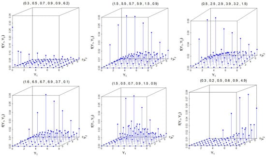
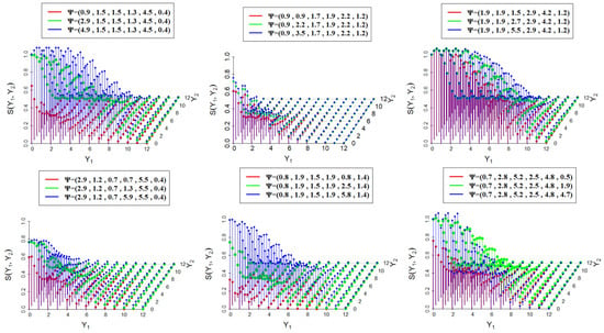
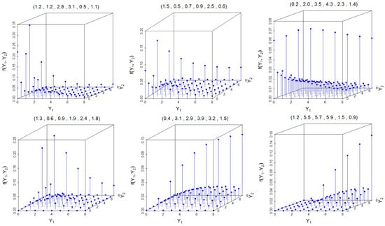
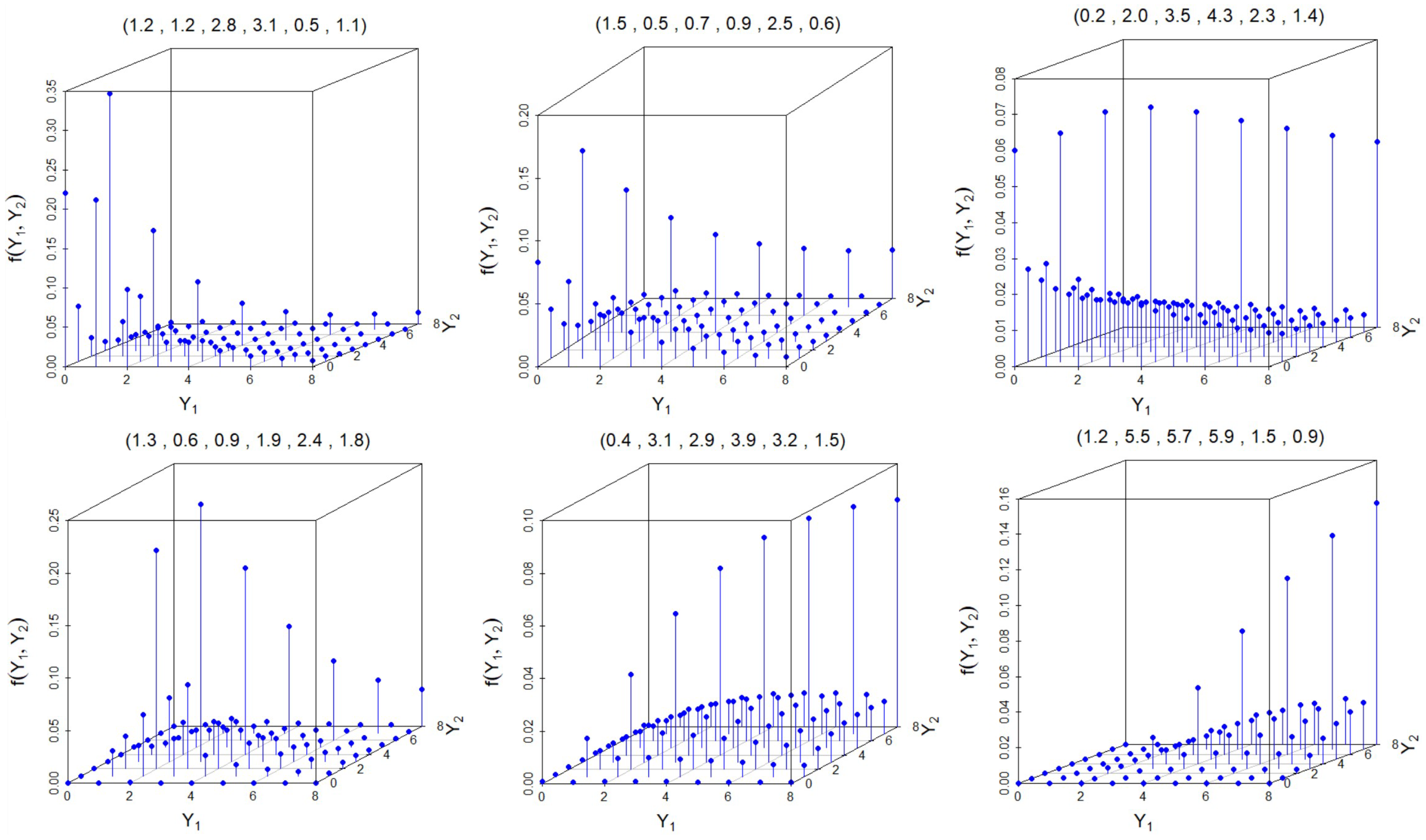
where $f_i(·)$ and $S_i(·)$ denote the PMF and SF of $U_i\sim \mathrm{WDFW}(\alpha ,{\beta }_i,m,k)$. Figure 1 and Figure 2 present scatter plots of the joint PMF and joint SF of the BWDFW-I model for various parameter values $(\alpha ,{\beta }_1,{\beta }_2,{\beta }_3,m,k)$.

Figure 1. The scatter plots of the joint PMF of the BWDFW-I model for different parameter values $(\alpha ,{\beta }_1,{\beta }_2,{\beta }_3,m,k)$.

Figure 2. The scatter plots of the joint SF of the BWDFW-I model for different parameter values $(\alpha ,{\beta }_1,{\beta }_2,{\beta }_3,m,k)$.

The PMF of the BWDFW-I model exhibits versatility in addressing and analyzing a broad range of data types. This model is particularly effective in representing data with varying distributional characteristics, including unimodal and multimodal structures, while accommodating asymmetry in the shape of the distribution. Such flexibility is critical in applications where data do not conform to standard symmetric patterns or exhibit multiple peaks, which are commonly observed in real-world scenarios across diverse fields.

Moreover, the BWDFW-I model provides a robust framework for handling specialized data scenarios, such as zero-inflated datasets with an excess of zero observations. This feature is crucial in many practical settings, including medical studies, ecological data, or quality-control processes, where zero inflation arises naturally because of underlying phenomena. Additionally, the model is equally adept at analyzing non-inflated datasets, thereby covering the entire spectrum of possible data structures. Another significant advantage of this model is its ability to perform reliably in the presence of outliers or extreme values. Such outliers often distort traditional analyses, leading to biased or misleading conclusions. The BWDFW-I model, with its inherent flexibility and well-defined mathematical structure, offers robust tools for mitigating the impacts of these anomalies. Consequently, it serves as an ideal choice for applications requiring robust statistical modeling under complex conditions, ensuring reliable insights, even in challenging datasets.

3.1.2. The Joint CDF of the BWDFW-I Model

The joint CDF, $(Y_1,Y_2)$, of the BWDFW-I model can be expressed using the relation

$$F_{Y_1,Y_2}(y_1,y_2)=F_{Y_1}\left(y_1\right)+F_{Y_2}\left(y_2\right)+S_{Y_1,Y_2}(y_1,y_2)-1,$$

(18)

where $F_{Y_1}\left(y_1\right)$ and $F_{Y_2}\left(y_2\right)$ represent the marginal CDFs $Y_1$ and $Y_2$, respectively, and $S_{Y_1,Y_2}(y_1,y_2)$ denotes the joint SF $(Y_1,Y_2)$ of the BWDFW-I model. The explicit form of the joint CDF, $F_{Y_1,Y_2}(y_1,y_2)$, of the BWDFW-I model is given by

$$\begin{array}{ccc}\hfill F_{Y_1,Y_2}(y_1,y_2;\Omega )& =& \left\{\begin{array}{cc}{F}_1(y_1,y_2;\Omega ),\hfill & y_1>y_2,\hfill \\ F_2(y_1,y_2;\Omega ),\hfill & y_2>y_1,\hfill \\ F_3(y;\Omega ),\hfill & y_1=y_2=y,\hfill \end{array}\right.\hfill \end{array}$$

where $F_1$, $F_2$, and $F_3$ represent different components of the joint CDF, depending on the relative magnitudes of $y_1$ and $y_2$. The first and second terms in Equation (18), corresponding to the marginal CDFs $Y_1$ and $Y_2$, are expressed as

$$F_{Y_i}\left(y_i\right)=1-S_{Y_i}\left(y_i\right)=1-\left\{S_i\left(y_i\right)S_3\left(y_i\right)\right\},i=1,2,$$

where $S_i(·)$ is the SF of $U_i\sim \mathrm{WDFW}(\alpha ,{\beta }_i,m,k)$.

3.1.3. The Joint HRF of the BWDFW-I Model

The joint HRF $(Y_1,Y_2)$, denoted by $h(y_1,y_2)$, can be expressed in terms of the joint PMF, $f(y_1,y_2)$, and the joint survival function (SF), $S(y_1,y_2)$, as follows:

$$h(y_1,y_2)={\displaystyle \frac{f(y_1,y_2)}{S(y_1,y_2)}}.$$

For the BWDFW-I model, the joint HRF, $h_{Y_1,Y_2}(y_1,y_2;\Omega )$, is defined piecewise based on the relationship between $y_1$ and $y_2$:

$$\begin{array}{ccc}\hfill h_{Y_1,Y_2}(y_1,y_2;\Omega )& =& \left\{\begin{array}{cc}{h}_1(y_1,y_2;\Omega ),\hfill & y_1>y_2,\hfill \\ h_2(y_1,y_2;\Omega ),\hfill & y_2>y_1,\hfill \\ h_3(y;\Omega ),\hfill & y_1=y_2=y.\hfill \end{array}\right.\hfill \end{array}$$

(19)

The terms $h_1(y_1,y_2;\Omega )$, $h_2(y_1,y_2;\Omega )$, and $h_3(y;\Omega )$ are further specified as follows:

$$h_i(y_1,y_2;\Omega )={\displaystyle \frac{f_i(y_1,y_2;\Omega )}{S_i(y_1,y_2;\Omega )}},(i=1,2),$$

and

$$h_3(y;\Omega )={\displaystyle \frac{f_3(y;\Omega )}{S_3(y;\Omega )}},$$

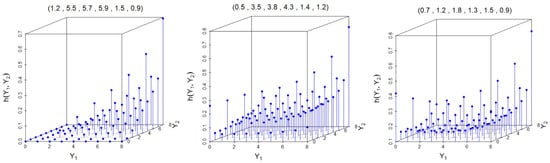
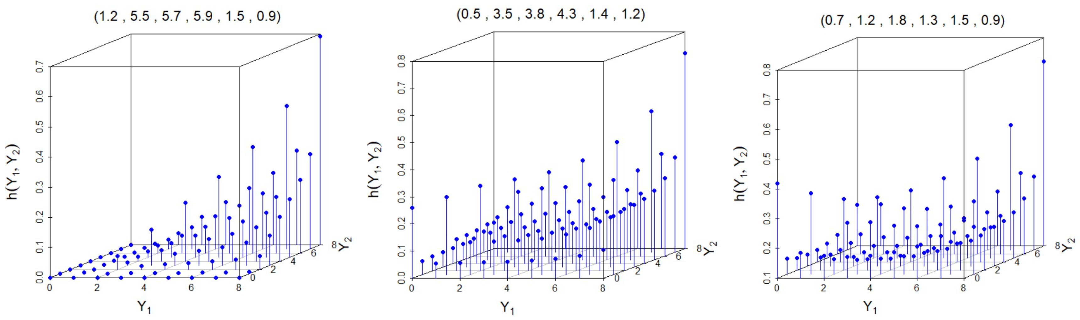
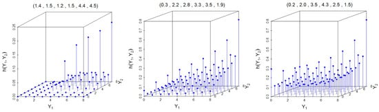
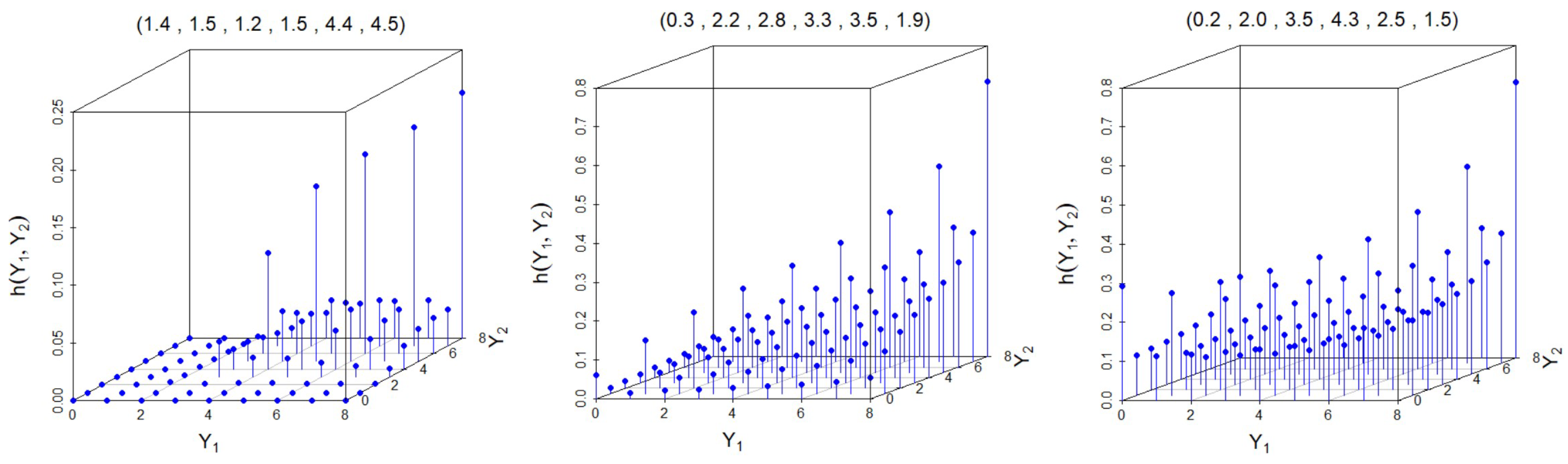
where $f_i(y_1,y_2;\Omega )$ and $S_i(y_1,y_2;\Omega )$ represent the PMF and SF for the corresponding components, as defined in Equation (14) and Equation (15), respectively. The various shapes of the joint HRF of the BWDFW-I model for various selections of model parameters are visually illustrated as scatter plots in Figure 3. This demonstrates the adaptability of the BWDFW-I distribution.

Figure 3. The scatter plots of the joint HRF of the BWDFW-I model for different parameter values $(\alpha ,{\beta }_1,{\beta }_2,{\beta }_3,m,k)$.

3.1.4. The Joint Reversed HRF of the BWDFW-I Model

The joint reversed hazard rate function (RHRF), $(Y_1,Y_2)$, of the BWDFW-I model is defined as follows:

$$\begin{array}{ccc}\hfill h_{Y_1,Y_2}^{*}(y_1,y_2;\Omega )& =& \left\{\begin{array}{cc}{h}_1^{*}(y_1,y_2;\Omega ),\hfill & y_1>y_2,\hfill \\ h_2^{*}(y_1,y_2;\Omega ),\hfill & y_2>y_1,\hfill \\ h_3^{*}(y;\Omega ),\hfill & y_1=y_2=y.\hfill \end{array}\right.\hfill \end{array}$$

(20)

The components of the RHRF, $h_1^{*}(y_1,y_2;\Omega )$, $h_2^{*}(y_1,y_2;\Omega )$, and $h_3^{*}(y;\Omega )$, are given by

$$h_1^{*}(y_1,y_2;\Omega )={\displaystyle \frac{f_1(y_1,y_2;\Omega )}{F_1(y_1,y_2;\Omega )}},h_2^{*}(y_1,y_2;\Omega )={\displaystyle \frac{f_2(y_1,y_2;\Omega )}{F_2(y_1,y_2;\Omega )}},\mathrm{and}{h}_3^{*}(y;\Omega )={\displaystyle \frac{f_3(y;\Omega )}{F_3(y;\Omega )}},$$

where $f_i(y_1,y_2;\Omega )$ and $F_i(y_1,y_2;\Omega )$ are the joint PMF and joint CDF of the BWDFW-I model, as defined in Equation (14) and Equation (18), respectively. The joint HRF and the joint RHRF of a bivariate model differ in their conditional interpretations and applications. The joint HRF measures the likelihood of the event pair $(Y_1,Y_2)$ occurring at specific values, given that no event has occurred up to those values, focusing on the “future” conditional risk. In contrast, the joint RHRF assesses the likelihood of the event pair $(Y_1,Y_2)$ occurring at specific values, given that the event has already occurred at or before those values, emphasizing the “past” conditional risk. The joint HRF is commonly used in survival analysis and reliability studies to predict future events, while the joint RHRF is relevant in reversed reliability analysis or retrospective studies to understand the likelihood of past events. These measures provide complementary perspectives, with the joint HRF focusing on the forward-looking risk and the joint RHRF on the retrospective likelihood.

3.2. The BWDFW Model Constructed Using the Maximum Operator

This section involves constructing and discussing the BWDFW distribution, using the maximum operator. Let us define $Y_1=max\{U_1,U_3\}$ and $Y_2=max\{U_2,U_3\}$, where $U_i\sim WDFW(\alpha ,{\beta }_i,m,k);(i=1,2,3)$, are independently distributed. By definition, the bivariate vector $\mathbf{Y}=(Y_1,Y_2)$ has a BWDFW distribution with the parameter vector $\Omega ={(\alpha ,{\beta }_1,{\beta }_2,{\beta }_3,m,k)}^T$. We denote the BWDFW distribution constructed using the maximum operator as BWDFW-II. Then, the joint PMF of $(Y_1,Y_2)\sim$ BWDFW-II is given by

$$\begin{array}{ccc}\hfill f_{Y_1,Y_2}(y_1,y_2;\Omega )& =& P[Y_1=y_1,Y_2=y_2;\Omega ]\hfill \\ & =& \left\{\begin{array}{cc}{f}_1(y_1,y_2;\Omega )\hfill & ;y_1>y_2,\hfill \\ f_2(y_1,y_2;\Omega )\hfill & ;y_1<y_2,\hfill \\ f_3(y;\Omega )\hfill & ;y_1=y_2=y,\hfill \end{array}\right.\hfill \end{array}$$

(21)

where

$$\begin{array}{ccc}\hfill f_1(y_1,y_2;\Omega )& =& f_1\left(y_1\right)\left\{f_2\left(y_2\right)F_3\left(y_2\right)+f_3\left(y_2\right)F_2(y_2-1)\right\};y_1>y_2,\hfill \\ \hfill f_2(y_1,y_2;\Omega )& =& f_2\left(y_2\right)\left\{f_1\left(y_1\right)F_3\left(y_1\right)+f_3\left(y_1\right)F_1(y_1-1)\right\};y_1<y_2,\hfill \\ \hfill f_3(y;\Omega )& =& f_3\left(y\right)F_2\left(y\right)F_1\left(y\right)+f_1\left(y\right)f_2\left(y\right)F_3(y-1);y_1=y_2=y,\hfill \end{array}$$

where $f_i(.)$ and $F_i(.)$ are the PMF and CDF of $U_i\sim$ WDFW$(\alpha ,{\beta }_i,m,k)$.

3.2.1. The Joint CDF of the BWDFW-II Model

The joint CDF of the $(Y_1,Y_2)\sim$ BWDFW-II model is given by

$$\begin{array}{ccc}\hfill F_{Y_1,Y_2}(y_1,y_2;\Omega )& =& P[Y_1\le y_1,Y_2\le y_2;\Omega ]\hfill \\ & =& P[max\{U_1,U_3\}\le y_1,max\{U_2,U_3\}\le y_2;\Omega ]\hfill \\ & =& \left\{\begin{array}{cc}{F}_1(y_1,y_2)\hfill & ;y_1>y_2,\hfill \\ F_2(y_1,y_2)\hfill & ;y_2>y_1,\hfill \\ F_3\left(y\right)\hfill & ;y_1=y_2=y.\hfill \end{array}\right.\hfill \end{array}$$

(22)

$F_1(y_1,y_2),F_1(y_1,y_2)$, and $F_3\left(y\right)$ are defined as follows:

$$\begin{array}{ccc}\hfill F_1(y_1,y_2)& =& F_1\left(y_1\right)F_2\left(y_2\right)F_3\left(y_2\right),\hfill \\ \hfill F_2(y_1,y_2)& =& F_1\left(y_1\right)F_2\left(y_2\right)F_3\left(y_1\right),\hfill \\ \hfill F_3\left(y\right)& =& F_1\left(y\right)F_2\left(y\right)F_3\left(y\right),\hfill \end{array}$$

where $F_i(.)$ is the cumulative distribution function of $U_i\sim$ WDFWD$(\alpha ,{\beta }_i,m,k)$, as defined in Equation (3). It is evident that the marginal CDF can be derived from the joint CDF as follows:

$$F_{Y_i}\left(y_i\right)=F_i\left(y_i\right)F_3\left(y_i\right);i=1,2.$$

(23)

The corresponding marginal PMF can be specified as

$$\begin{array}{ccc}\hfill f_{Y_i}\left(y_i\right)& =& F_{Y_i}(y_i+1)-F_{Y_i}\left(y_i\right)\hfill \\ & =& F_i(y_i+1)F_3(y_i+1)+F_i\left(y_i\right)F_3\left(y_i\right)\hfill \\ & =& f_i\left(y_i\right)F_3\left(y_i\right)+f_3\left(y_i\right)F_i(y_i+1);y_i\ge 0(i=1,2),\hfill \end{array}$$

(24)

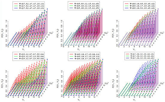
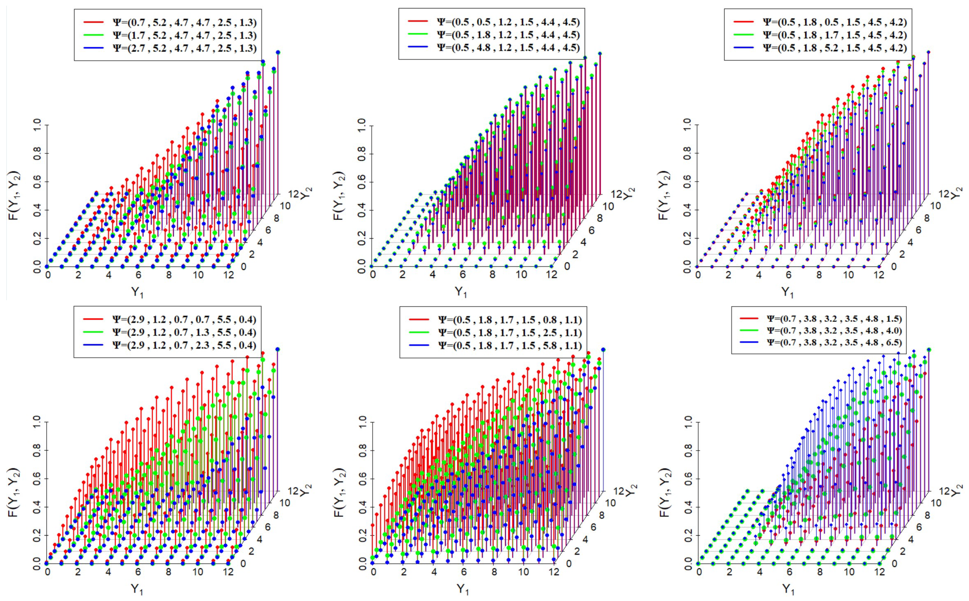
where $f_i(.)$ and $F_i(.)$ are the PMF and CDF of $U_i\sim$ WDFW$(\alpha ,{\beta }_i,m,k)$. Figure 4 and Figure 5 represent the scatter plots of the joint PMF and joint CDF of the BWDFW-II model for different parameter values $(\alpha ,{\beta }_1,{\beta }_2,{\beta }_3,m,k)$. These plots reveal that the joint PMF of the BWDFW-II model exhibits considerable flexibility, assuming diverse shapes based on the parameter values $(\alpha ,{\beta }_1,{\beta }_2,{\beta }_3,m,k)$. Notably, the joint mass can display both long left and long right tails, highlighting its adaptability in capturing various distributional behaviors. This flexibility extends to scenarios involving zero-inflated and non-zero-inflated structures, accommodating excess zeros or the absence thereof in the data. The plots of the CDF illustrate the adaptability of the joint CDF through its wide range of possible shapes, further emphasizing the model’s robustness in handling different data patterns, including those with and without zero-inflation.

Figure 4. The scatter plots of the joint PMF of the BWDFW-II model for different parameter values $(\alpha ,{\beta }_1,{\beta }_2,{\beta }_3,m,k)$.

Figure 5. The scatter plots of the joint CDF of the BWDFW-II model for different parameter values $(\alpha ,{\beta }_1,{\beta }_2,{\beta }_3,m,k)$.

3.2.2. The Joint SF of the BWDFW-II Model

The joint SF, $(Y_1,Y_2)$, of the BWDFW-II model can be derived using the following relation:

$$S_{Y_1,Y_2}(y_1,y_2)=1-F_{Y_1}\left(y_1\right)-F_{Y_2}\left(y_2\right)+F_{Y_1,Y_2}(y_1,y_2).$$

(25)

Thus, the joint SF of the BWDFW-II model can be formulated as

$$\begin{array}{ccc}\hfill S_{Y_1,Y_2}(y_1,y_2;\Omega )& =& \left\{\begin{array}{cc}{S}_1(y_1,y_2;\Omega )\hfill & ;y_1>y_2,\hfill \\ S_2(y_1,y_2;\Omega )\hfill & ;y_2>y_1,\hfill \\ S_3(y;\Omega )\hfill & ;y_1=y_2=y.\hfill \end{array}\right.\hfill \end{array}$$

The second and third terms of Equation (25) represent the marginal cumulative distribution functions (CDFs) $Y_1$ and $Y_2$, respectively, as defined in Equation (23). The fourth term, $F_{Y_1,Y_2}(y_1,y_2)$, corresponds to the joint CDF of the BWDFW-II model. Other reliability characteristics, such as the joint hazard rate function and the joint reversed hazard rate function of the BWDFW-II model, can be expressed analogously to those of the BWDFW-I model but are formulated based on Equations (21), (22), and (25), respectively.

Figure 6 presents scatter plots that illustrate the joint HRF of the BWDFW-II model in various parameter configurations. The different shapes of these joint HRF information graphics highlight the flexibility of the model.

Figure 6. The scatter plots of the joint HRF of the BWDFW-II model for different parameter values $(\alpha ,{\beta }_1,{\beta }_2,{\beta }_3,m,k)$.

4. Positive Quadrant Dependence

Positive quadrant dependence (PQD) is a concept that characterizes the relationship between two random variables when they tend to be simultaneously small or large. It represents a form of dependence where the probability of both random variables being small or large together is at least as high as it would be if they were independent. PQD implies that when one variable takes on a higher value, the likelihood of the other variable also being higher increases. Although PQD indicates positive dependence between the bivariate random variables $Y_1$ and $Y_2$, it does not necessarily imply that their correlation is always positive. PQD is particularly important in areas such as finance and reliability analysis, as it helps in understanding the dependencies between variables, which is crucial for effective modeling and prediction. In this section, we demonstrate that both the BWDFW-I and BWDFW-II models exhibit PQD. As a result, a bivariate random pair ($(Y_1,Y_2)$) from either the BWDFW-I or BWDFW-II model shows positive dependence.

Theorem 3. 

If the $(Y_1,Y_2)\sim$ BWDFW-I model, with parameters $(\alpha ,{\beta }_1,{\beta }_2,{\beta }_3,m,k)$, such that $Y_1=min\{U_1,U_3\}$ and $Y_1=min\{U_1,U_3\}$, where $U_1,U_2$, and $U_3$ are the baseline random variables, then $Y_1$ and $Y_2$ are $PQD$.

Proof. 

Let $U_i\sim$ WDFW $(\alpha ,{\beta }_i,m,k)$ be the baseline distribution for $Y_1$ and $Y_2$, such that $Y_1=min\{U_1,U_3\}$ and $Y_1=min\{U_1,U_3\}$. Then, by definition, $(Y_1,Y_2)\sim$ the BWDFW-I model, with the parameter set $(\alpha ,{\beta }_1,{\beta }_2,{\beta }_3,m,k)$. And to prove that $Y_1$ and $Y_2$ are PQD, it is sufficient to prove the inequality

$$P(Y_1>y_1,Y_2>y_2)\ge P(Y_1>y_1)P(Y_2>y_2);\forall y_1,y_2.$$

(26)

Considering the right-hand side of Equation (26),

$$\begin{array}{ccc}\hfill P(Y_1>y_1)P(Y_2>y_2)& =& S_1\left(y_1\right)S_2\left(y_2\right)\hfill \\ & =& S_1\left(y_1\right)S_3\left(y_1\right)S_2\left(y_2\right)S_3\left(y_2\right).\hfill \end{array}$$

(27)

Now, for the left-hand side of Equation (26), we need to consider two cases as follows:

Case 1: 

$y_1\ge y_2$

$$\begin{array}{ccc}\hfill P(Y_1>y_1,Y_2>y_2)& =& S_{Y_1,Y_2}(y_1,y_2){|}_{y_1\ge y_2}\hfill \\ & =& S_1\left(y_1\right)S_2\left(y_2\right)S_3\left(y_1\right).\hfill \end{array}$$

(28)

Case 2: 

$y_1<y_2$

$$\begin{array}{ccc}\hfill P(Y_1>y_1,Y_2>y_2)& =& S_{Y_1,Y_2}(y_1,y_2){|}_{y_2>y_1}\hfill \\ & =& S_1\left(y_1\right)S_2\left(y_2\right)S_3\left(y_2\right).\hfill \end{array}$$

(29)

It is clearly seen that Equation (28) ≥ Equation (27), and Equation (29) ≥ Equation (27). Thus, the result. □

Theorem 4. 

If $(Y_1,Y_2)\sim$ the BWDFW-II model, such that $Y_1=max\{U_1,U_3\}$ and $Y_1=max\{U_1,U_3\}$, where $U_1,U_2$, and $U_3$ are the baseline random variables, then $Y_1$ and $Y_2$ are PQD.

Proof. 

If $(Y_1,Y_2)\sim$ the BWDFW-II model, with parameters $(\alpha ,{\beta }_1,{\beta }_2,{\beta }_3,m,k)$, then, to prove that $Y_1$ and $Y_2$ are $PQD$, it is sufficient to prove the inequality

$$P(Y_1\le y_1,Y_2\le y_2)\ge P(Y_1\le y_1)P(Y_2\le y_2);\forall y_1,y_2.$$

(30)

Considering the right-hand side of Equation (30),

$$P(Y_1\le y_1)P(Y_2\le y_2)=F_1\left(y_1\right)F_3\left(y_1\right)F_2\left(y_2\right)F_3\left(y_2\right).$$

(31)

Now, for the left-hand side of Equation (30), we need to consider two cases as follows:

Case 1: 

$y_1\le y_2$

$$P(Y_1\le y_1,Y_2\le y_2)=F_1\left(y_1\right)F_2\left(y_2\right)F_3\left(y_2\right).$$

(32)

Case 2: 

$y_1<y_2$

$$P(Y_1\le y_1,Y_2\le y_2)=F_1\left(y_1\right)F_2\left(y_2\right)F_3\left(y_1\right).$$

(33)

It is clearly seen that Equation (32) ≥ Equation (31), and Equation (33) ≥ Equation (31). Thus, the result. □

5. The Joint Probability-Generating Function Along with Associated Measures

If the bivariate vector, $(Y_1,Y_2),\sim$ the BWDFW-I model with parameter set $(\alpha ,{\beta }_1,{\beta }_2,{\beta }_3,m,k)$, then the joint probability-generating function (PGF) of $Y_1$ and $Y_2$ for $|t_1|<1$ and $|t_2|<1$ can be written as

$$\begin{array}{cc}\hfill G_{Y_1,Y_2}(t_1,t_2)& =E\left(t_1^{Y_1}{t}_2^{Y_2}\right)\hfill \\ \hfill & =\sum _{j,i=0}^{\infty }P[Y_1=i,Y_2=j]t_1^i{t}_2^j\hfill \\ \hfill & =\sum _{j=0}^{\infty }\sum _{i=0}^{j-1}{f}_1(y_1,y_2;\Omega )t_1^i{t}_2^j+\sum _{j=0}^{\infty }\sum _{i=j+1}^{\infty }{f}_1(y_1,y_2;\Omega )t_1^i{t}_2^j\hfill \\ \hfill & +\sum _{i=0}^{\infty }{f}_3(y;\Omega )t_1^i{t}_2^i;|t_1|,|t_2|<1,\hfill \end{array}$$

(34)

where $f_1(y_1,y_2;\Omega )$, $f_2(y_1,y_2;\Omega )$, and $f_3(y;\Omega )$ are the joint PMF of the BWDFW-I model, as defined in Equation (14).

Similarly, the joint PGF of the BWDFW-II model can also be expressed, where $f_1(y_1,y_2;\Omega )$, $f_2(y_1,y_2;\Omega )$, and $f_3(y;\Omega )$ represent the joint PMF of the BWDFW-II model, as defined in Equation (21). It is widely recognized that the joint PGF serves as a valuable tool for deriving various moments and product moments. Utilizing this joint PGF in the BWDFW-I and BWDFW-II models, different factorial moments, raw moments, and product moments can be represented as infinite series. For a bivariate vector, $(Y_1,Y_2)$, taking the partial derivative of the joint PGF $G_{Y_1,Y_2}(t_1,t_2)$ with respect to $t_i$ for r times gives the $r^{th}$ factorial moment of $Y_i$ (where $i=1,2$). This can be expressed as follows:

$${{\mu }_{Y_i}^{\prime }}_{\left(r\right)}={\displaystyle \frac{{\partial }^r}{\partial t_i^r}}{G}_{Y_1,Y_2}(t_1,t_2){|}_{t_1=1,t_2=1};i=1,2,$$

(35)

where ${{\mu }_{Y_i}^{\prime }}_{\left(r\right)}$ is the $r^{th}$ factorial moment of $Y_i;(i=1,2)$. Taking the first and second partial derivatives of Equation (35) with respect to “$t_i$” and substituting in $t_1=1 \mathrm{and} t_2=1$, respectively, yields the following relations:

$$\begin{array}{ccc}\hfill {{\mu }_{Y_i}^{\prime }}_{\left(1\right)}& =& {\displaystyle \frac{\partial }{\partial t_i}}{G}_{Y_1,Y_2}(t_1,t_2){|}_{t_1=1,t_2=1}=E\left(Y_i\right),\hfill \\ \hfill {{\mu }_{Y_i}^{\prime }}_{\left(2\right)}& =& {\displaystyle \frac{{\partial }^2}{\partial t_i^2}}{G}_{Y_1,Y_2}(t_1,t_2){|}_{t_1=1,t_2=1}.\hfill \end{array}$$

(36)

Similarly, from Equation (35), we can have

$$E\left(Y_1{Y}_2\right)={\displaystyle \frac{{\partial }^2}{\partial t_1\partial t_2}}{G}_{Y_1,Y_2}(t_1,t_2){|}_{t_1=1,t_2=1}.$$

Thus, the variances $Y_i(i=1,2)$ and the covariance $(Y_1,Y_2)$ can be obtained using the relations

$$\begin{array}{ccc}\hfill Var\left(Y_i\right)& =& {{\mu }_{Y_i}^{\prime }}_{\left(2\right)}+{{\mu }_{Y_i}^{\prime }}_{\left(1\right)}-{\left\{{{\mu }_{Y_i}^{\prime }}_{\left(1\right)}\right\}}^2,\hfill \end{array}$$

(37)

$$\begin{array}{ccc}\hfill Cov(Y_1,Y_2)& =& E\left(Y_1{Y}_2\right)-{{\mu }_{Y_1}^{\prime }}_{\left(1\right)}{{\mu }_{Y_2}^{\prime }}_{\left(1\right)}.\hfill \end{array}$$

(38)

Table 1 presents the descriptive statistics for a randomly selected pair ($Y_1,Y_2$) generated from the BWDFW-I model, including an analysis of covariance, Pearson’s correlation coefficient, Spearman’s rho ($\rho$), and Kendall’s tau ($\tau$). Likewise, Table 2 provides the corresponding values for the BWDFW-II model.

Table 1. Some descriptive statistics for the BWDFW-I model.

$\mathit{\alpha }$	${\mathit{\beta }}_1$	${\mathit{\beta }}_2$	${\mathit{\beta }}_3$	m	k	Cov(${\mathit{Y}}_1,{\mathit{Y}}_2$)	Cor(${\mathit{Y}}_1,{\mathit{Y}}_2$)	$\mathit{\rho }$(${\mathit{Y}}_1,{\mathit{Y}}_2$)	$\mathit{\tau }$(${\mathit{Y}}_1,{\mathit{Y}}_2$)
0.5	4.5	2.5	6.4	2.5	7.5	2.39225	0.96608	0.90881	0.87911
0.9						0.46123	0.85967	0.82312	0.80758
1.7						0.13837	0.53373	0.50025	0.49463
0.7	1.7	2.3	6.0	2.7	7.2	1.07347	0.92541	0.85927	0.83332
	4.5					1.14286	0.90563	0.81902	0.78072
	6.0					1.18204	0.90642	0.78258	0.74836
1.8	4.0	2.5	5.2	3.5	6.5	0.17551	0.61911	0.58162	0.55979
		4.5				0.12939	0.79906	0.69577	0.68757
		6.0				0.28939	0.82651	0.87992	0.86742
1.5	5.2	2.4	3.8	2.6	5.1	0.11673	0.54648	0.53101	0.51852
			4.8			0.12490	0.51522	0.48029	0.46688
			5.2			0.17551	0.59312	0.52037	0.50695
1.3	5.4	2.5	3.5	2.4	5.5	0.29918	0.73049	0.66068	0.64165
				3.5		0.44898	0.80526	0.74152	0.70841
				4.5		0.78928	0.87736	0.82274	0.78307
1.7	4.5	3.2	4.2	2.7	2.5	1.71511	0.96606	0.95796	0.92875
					4.0	0.33347	0.72678	0.66341	0.63503
					7.2	0.01633	0.14744	0.14744	0.14744

Table 2. Some descriptive statistics for the BWDFW-II model.

$\mathit{\alpha }$	${\mathit{\beta }}_1$	${\mathit{\beta }}_2$	${\mathit{\beta }}_3$	m	k	Cov(${\mathit{Y}}_1,{\mathit{Y}}_2$)	Cor(${\mathit{Y}}_1,{\mathit{Y}}_2$)	$\mathit{\rho }$(${\mathit{Y}}_1,{\mathit{Y}}_2$)	$\mathit{\tau }$(${\mathit{Y}}_1,{\mathit{Y}}_2$)
0.6	3.8	5.5	4.2	1.9	5.6	3.04980	0.98617	0.97905	0.96399
1.3						1.56408	0.89377	0.90127	0.89458
1.8						0.53061	0.93037	0.92779	0.92758
0.8	1.5	4.5	3.4	1.5	6.2	0.30082	0.82114	0.80861	0.79306
	2.4					0.37755	0.95183	0.96047	0.95197
	3.2					0.40735	0.97604	0.96826	0.96753
1.5	0.9	1.5	3.0	2.7	4.1	0.35918	0.75211	0.69959	0.66731
		2.7				0.48980	0.88828	0.89514	0.85235
		3.2				0.46939	0.90915	0.93774	0.90086
1.2	0.9	2.7	1.3	2.5	4.5	0.18491	0.67127	0.59604	0.58744
			2.2			0.22908	0.73535	0.63395	0.61371
			2.9			0.23306	0.75522	0.67167	0.65002
2.2	1.8	1.9	2.8	1.5	3.4	0.29918	0.73049	0.66068	0.64165
				2.4		0.44898	0.80526	0.74152	0.70841
				3.3		0.78928	0.87736	0.82274	0.78307
1.9	1.7	2.3	2.4	2.3	2.7	0.85878	0.88365	0.84753	0.79743
					3.5	0.51265	0.82018	0.79669	0.78712
					4.4	0.22082	0.75264	0.76424	0.74579

From Table 1 and Table 2, it is evident that for both the BWDFW-I and BWDFW-II models, the values of covariance, correlation, Spearman’s rho, and Kendall’s tau are greater than zero. This observation directly reflects the property of the PQD.

6. The Maximum Likelihood Estimation

Let us consider a bivariate sample of size n of the form $\{(y_{11},y_{21}),(y_{12},y_{22}),\dots ,(y_{1n},y_{2n})\}$ from the BWDFW-I model. Now, to estimate the values of the unknown parameters ($\alpha ,{\beta }_1,{\beta }_2,{\beta }_3,$$m,k$) of the BWDFW-I model, using the maximum likelihood estimation (MLE) method, let us assume $I_1=\{y_{1j}<y_{2j}\}$, $I_2=\{y_{1j}>y_{2j}\}$, and $I_3=\{y_{1j}=y_{2j}=y_j\}$, such that $I=I_1\cup I_2\cup I_3$. Also, let the numbers of elements in $I_1$, $I_2$, and $I_3$ be $n_1$, $n_2$, and $n_3$, respectively, such that $n=n_1+n_2+n_3$. Using these notations, for the parameter vector $\Omega ={(\alpha ,{\beta }_1,{\beta }_2,{\beta }_3,m,k)}^T$, the likelihood function of the BWDFW-I model is given by

$$L(\Omega )=\prod _{j=1}^{n_1}{f}_1(y_{1j},y_{2j};\Omega )\prod _{j=1}^{n_2}{f}_2(y_{1j},y_{2j};\Omega )\prod _{j=1}^{n_3}{f}_3(y_j;\Omega ).$$

Then, the log-likelihood function can be formulated as

$$l(\Omega )=\sum _{j=1}^{n_1}ln{f}_1(y_{1j},y_{2j};\Omega )+\sum _{j=1}^{n_2}ln{f}_2(y_{1j},y_{2j};\Omega )+\sum _{j=1}^{n_3}ln{f}_3(y_j;\Omega ),$$

(39)

where $f_1(y_{1j},y_{2j};\Omega ),f_2(y_{1j},y_{2j};\Omega )$, and $f_3(y_j;\Omega )$ are the joint PMF cases of the BWDFW-I model, as defined in Equation (14). The MLE of parameters $\alpha ,{\beta }_1,{\beta }_2,{\beta }_3,m$, and k can be obtained by solving the partial derivatives of Equation (39) with respect to $\alpha ,{\beta }_1,{\beta }_2,{\beta }_3,m$, and k and then equating the results to zero. The partial derivatives are expressed as follows:

$$\begin{array}{ccc}\hfill {\displaystyle \frac{\partial l}{\partial \alpha }}& =& {\displaystyle \frac{\partial l_1}{\partial \alpha }}+{\displaystyle \frac{\partial l_2}{\partial \alpha }}+{\displaystyle \frac{\partial l_3}{\partial \alpha }},\hfill \\ \hfill {\displaystyle \frac{\partial l_1}{\partial \alpha }}& =& \sum _{j=1}^{n_1}{\psi }_1(y_{2j};\alpha ,{\beta }_2,m,k)[\left\{{\psi }_1(y_{1j};\alpha ,{\beta }_1,m,k)\times {\psi }_2(y_{1j}-1;\alpha ,{\beta }_3,m,k)\right\}\hfill \\ & & +\left\{{\psi }_1(y_{1j};\alpha ,{\beta }_3,m,k)\times {\psi }_2(y_{1j};\alpha ,{\beta }_1,m,k)\right\}],\hfill \\ \hfill {\displaystyle \frac{\partial l_2}{\partial \alpha }}& =& \sum _{j=1}^{n_2}{\psi }_1(y_{1j};\alpha ,{\beta }_1,m,k)[\left\{{\psi }_1(y_{2j};\alpha ,{\beta }_2,m,k)\times {\psi }_2(y_{2j}-1;\alpha ,{\beta }_3,m,k)\right\}\hfill \\ & & +\left\{{\psi }_1(y_{2j};\alpha ,{\beta }_3,m,k)\times {\psi }_2(y_{2j};\alpha ,{\beta }_2,m,k)\right\}],\hfill \\ \hfill {\displaystyle \frac{\partial l_3}{\partial \alpha }}& =& \sum _{j=1}^{n_3}[\left\{{\psi }_1(y_j;\alpha ,{\beta }_3,m,k)\times {\psi }_2(y_j-1;\alpha ,{\beta }_2,m,k)\times {\psi }_2(y_j-1;\alpha ,{\beta }_1,m,k)\right\}\hfill \\ & & +\left\{{\psi }_1(y_j;\alpha ,{\beta }_1,m,k)\times {\psi }_1(y_j;\alpha ,{\beta }_2,m,k)\times {\psi }_2(y_j;\alpha ,{\beta }_3,m,k)\right\}].\hfill \end{array}$$

$$\begin{array}{ccc}\hfill {\displaystyle \frac{\partial l}{\partial m}}& =& {\displaystyle \frac{\partial l_1}{\partial m}}+{\displaystyle \frac{\partial l_2}{\partial m}}+{\displaystyle \frac{\partial l_3}{\partial m}},\hfill \\ \hfill {\displaystyle \frac{\partial l_1}{\partial m}}& =& \sum _{j=1}^{n_1}{\mathsf{\Psi }}_1(y_{2j};\alpha ,{\beta }_2,m,k)[\left\{{\mathsf{\Psi }}_1(y_{1j};\alpha ,{\beta }_1,m,k)\times {\mathsf{\Psi }}_2(y_{1j}-1;\alpha ,{\beta }_3,m,k)\right\}\hfill \\ & & +\left\{{\mathsf{\Psi }}_1(y_{1j};\alpha ,{\beta }_3,m,k)\times {\mathsf{\Psi }}_2(y_{1j};\alpha ,{\beta }_1,m,k)\right\}],\hfill \\ \hfill {\displaystyle \frac{\partial l_2}{\partial m}}& =& \sum _{j=1}^{n_2}{\mathsf{\Psi }}_1(y_{1j};\alpha ,{\beta }_1,m,k)[\left\{{\mathsf{\Psi }}_1(y_{2j};\alpha ,{\beta }_2,m,k)\times {\mathsf{\Psi }}_2(y_{2j}-1;\alpha ,{\beta }_3,m,k)\right\}\hfill \\ & & +\left\{{\mathsf{\Psi }}_1(y_{2j};\alpha ,{\beta }_3,m,k)\times {\mathsf{\Psi }}_2(y_{2j};\alpha ,{\beta }_2,m,k)\right\}],\hfill \\ \hfill {\displaystyle \frac{\partial l_3}{\partial m}}& =& \sum _{j=1}^{n_3}[\left\{{\mathsf{\Psi }}_1(y_j;\alpha ,{\beta }_3,m,k)\times {\mathsf{\Psi }}_2(y_j-1;\alpha ,{\beta }_2,m,k)\times {\mathsf{\Psi }}_2(y_j-1;\alpha ,{\beta }_1,m,k)\right\}\hfill \\ & & +\left\{{\mathsf{\Psi }}_1(y_j;\alpha ,{\beta }_1,m,k)\times {\mathsf{\Psi }}_1(y_j;\alpha ,{\beta }_2,m,k)\times {\mathsf{\Psi }}_2(y_j;\alpha ,{\beta }_3,m,k)\right\}].\hfill \end{array}$$

$$\begin{array}{ccc}\hfill {\displaystyle \frac{\partial l}{\partial k}}& =& {\displaystyle \frac{\partial l_1}{\partial k}}+{\displaystyle \frac{\partial l_2}{\partial k}}+{\displaystyle \frac{\partial l_3}{\partial k}},\hfill \\ \hfill {\displaystyle \frac{\partial l_1}{\partial k}}& =& \sum _{j=1}^{n_1}{\mathsf{\Phi }}_1(y_{2j};\alpha ,{\beta }_2,m,k)[\left\{{\mathsf{\Phi }}_1(y_{1j};\alpha ,{\beta }_1,m,k)\times {\mathsf{\Phi }}_2(y_{1j}-1;\alpha ,{\beta }_3,m,k)\right\}\hfill \\ & & +\left\{{\mathsf{\Phi }}_1(y_{1j};\alpha ,{\beta }_3,m,k)\times {\mathsf{\Phi }}_2(y_{1j};\alpha ,{\beta }_1,m,k)\right\}],\hfill \\ \hfill {\displaystyle \frac{\partial l_2}{\partial k}}& =& \sum _{j=1}^{n_2}{\mathsf{\Phi }}_1(y_{1j};\alpha ,{\beta }_1,m,k)[\left\{{\mathsf{\Phi }}_1(y_{2j};\alpha ,{\beta }_2,m,k)\times {\mathsf{\Phi }}_2(y_{2j}-1;\alpha ,{\beta }_3,m,k)\right\}\hfill \\ & & +\left\{{\mathsf{\Phi }}_1(y_{2j};\alpha ,{\beta }_3,m,k)\times {\mathsf{\Phi }}_2(y_{2j};\alpha ,{\beta }_2,m,k)\right\}],\hfill \\ \hfill {\displaystyle \frac{\partial l_3}{\partial k}}& =& \sum _{j=1}^{n_3}[\left\{{\mathsf{\Phi }}_1(y_j;\alpha ,{\beta }_3,m,k)\times {\mathsf{\Phi }}_2(y_j-1;\alpha ,{\beta }_2,m,k)\times {\mathsf{\Phi }}_2(y_j-1;\alpha ,{\beta }_1,m,k)\right\}\hfill \\ & & +\left\{{\mathsf{\Phi }}_1(y_j;\alpha ,{\beta }_1,m,k)\times {\mathsf{\Phi }}_1(y_j;\alpha ,{\beta }_2,m,k)\times {\mathsf{\Phi }}_2(y_j;\alpha ,{\beta }_3,m,k)\right\}].\hfill \end{array}$$

${\psi }_1\left(y\right),{\psi }_2\left(y\right),{\mathsf{\Psi }}_1\left(y\right),{\mathsf{\Psi }}_2\left(y\right),{\mathsf{\Phi }}_1\left(y\right)$, and ${\mathsf{\Phi }}_2\left(y\right)$ are defined as follows:

$$\begin{array}{ccc}\hfill {\psi }_1(y;\alpha ,{\beta }_i,m,k)& =& {\displaystyle \frac{E_i(y_j+1)F_i(y_j+1)-E_i\left(y_j\right)F_i\left(y_j\right)}{{\left[G_i\left(y_j\right)\right]}^2}},\hfill \\ \hfill {\psi }_2(y;\alpha ,{\beta }_i,m,k)& =& -{\psi }_1(y;\alpha ,{\beta }_i,m,k),\hfill \\ \hfill {\mathsf{\Psi }}_1(y;\alpha ,{\beta }_i,m,k)& =& m^{-1}{\displaystyle \frac{A_i\left(y_j\right)B_i\left(y_j\right)}{D_i\left(y_j\right)}}+{\displaystyle \frac{E_i(y_j+1)H_i(y_j+1)-E_i\left(y_j\right)H_i\left(y_j\right)}{{\left[G_i\left(y_j\right)\right]}^2}},\hfill \\ \hfill {\mathsf{\Psi }}_2(y;\alpha ,{\beta }_i,m,k)& =& -{\mathsf{\Psi }}_1(y;\alpha ,{\beta }_i,m,k),\hfill \\ \hfill {\mathsf{\Phi }}_1(y;\alpha ,{\beta }_i,m,k)& =& {\displaystyle \frac{A_i\left(y_j\right)B_i\left(y_j\right)C_i\left(y_j\right)}{D_i\left(y_j\right)}}+{\displaystyle \frac{E_i(y_j+1)I_i(y_j+1)-E_i\left(y_j\right)I_i\left(y_j\right)}{{\left[G_i\left(y_j\right)\right]}^2}},\hfill \\ \hfill {\mathsf{\Phi }}_2(y;\alpha ,{\beta }_i,m,k)& =& -{\mathsf{\Phi }}_1(y;\alpha ,{\beta }_i,m,k),\hfill \end{array}$$

whereas $A_i\left(y\right),B_i\left(y\right),C_i\left(y\right),D_i\left(y\right),E_i\left(y\right),F_i\left(y\right),G_i\left(y\right),H_i\left(y\right)$, and $I_i\left(y\right)$ are defined as follows:

$$\begin{array}{cccc}\hfill A\left(y_i\right)& =exp\left\{-{\left({\displaystyle \frac{y_i+1}{m}}\right)}^k\right\},\hfill & \hfill B\left(y_i\right)& ={\left({\displaystyle \frac{y_i+1}{m}}\right)}^k,\hfill \\ \hfill C\left(y_i\right)& =lo{g}_e\left({\displaystyle \frac{y_i+1}{m}}\right),\hfill & \hfill D\left(y_i\right)& =1-exp\left\{-{\left({\displaystyle \frac{y_i+1}{m}}\right)}^k\right\},\hfill \\ \hfill E\left(y_i\right)& =exp\left\{-{\beta }^{\alpha }{\left({\displaystyle \frac{m}{y_i}}\right)}^{\alpha k}\right\},\hfill & \hfill F\left(y_i\right)& ={\left\{-\alpha \beta {\left({\displaystyle \frac{m}{y_i}}\right)}^k\right\}}^{\alpha -1},\hfill \\ \hfill H\left(y_i\right)& =-\alpha k{\beta }^{\alpha }{m}^{\alpha k-1}{y}^{-\alpha k},\hfill & \hfill I\left(y_i\right)& =-{\alpha }^2{\beta }^{\alpha }k{\left({\displaystyle \frac{m}{y_i}}\right)}^{\alpha k-1},\hfill \end{array}$$

and

$$G\left(y_i\right)=P[Y=y_i]=exp\left\{-{\beta }^{\alpha }{\left({\displaystyle \frac{m}{y+1}}\right)}^{\alpha k}\right\}-exp\left\{-{\beta }^{\alpha }{\left({\displaystyle \frac{m}{y}}\right)}^{\alpha k}\right\}.$$

These equations are not easy to solve. We need a numerical technique for the maximum likelihood estimators, like the Newton–Raphson method. The log-likelihood function can similarly be expressed for the BWDFW-II model by considering the cases in the joint PMF, as given by Equation (21). For both models, we used the statistical package “MLE” in R-programming software Version 5 to obtain the maximum likelihood estimates.

7. Simulation: Behaviors of Estimators

Bivariate discrete data generation is crucial in statistical modeling, particularly for real-world applications in medical, engineering, and reliability studies. The BWDFW-I and BWDFW-II models offer enhanced flexibility in capturing overdispersion, skewness, and dependency structures in discrete count data. To assess the performances of their MLEs, a simulation study was conducted using the stats4 package version 5 in R. This section describes the data generation process for these models, considering various sample sizes ($n=50,80,120,150,$ and 200). Parameter values ($\alpha ,{\beta }_1,{\beta }_2,{\beta }_3,m,$ and k) were generated with 1000 replications, demonstrating the models’ practical significance.

7.1. Generation Process of Bivariate Discrete Data

The generation of bivariate discrete data from BWDFW-I and BWDFW-II follows a structured methodology:

Step 1: Define the marginal distributions. Both BWDFW-I and BWDFW-II versions define marginal probability mass functions (PMFs) for each variable.

Step 2: Construct the bivariate joint distribution. To introduce dependency, a copula-based or conditional sampling approach is applied. The joint probability function can be modeled as follows:

$$P(X=x,Y=y)=C(F_X\left(x\right),F_Y\left(y\right);\rho ),$$

where $C(·,·;\rho )$ represents a suitable copula function incorporating correlation $\rho$ into the model dependency.

Step 3: Generate random samples. For various sample sizes ($n=50,80,120,150,$ and 200), the following steps are executed:

• Generate uniform random variables $U_1,U_2$ from $U(0,1)$.
• Transform these uniform variables using the inverse CDF method:

  $$X=F_X^{-1}\left(U_1\right),Y=F_Y^{-1}\left(U_2\right),$$

  where $F_X^{-1}$ and $F_Y^{-1}$ are the inverse CDFs of BWDFW-I and BWDFW-II.
• Apply a copula-based transformation if a dependency structure is required.
• Repeat this process until the desired sample size is achieved.

7.2. Sample Size Considerations and Importance

The choice of the sample size significantly impacts the accuracy and reliability of the statistical inference:

• Small samples ($n=50,n=80$) are suitable for preliminary analysis, small samples’ property testing, and exploratory data assessment;
• Medium samples ($n=120,n=150$) provide more stability in parameter estimation and model validation;
• Large samples ($n=200$) allow for robust inferential procedures, including hypothesis testing and model selection.

7.3. The Accuracy and Precision of the Estimation Method

The accuracy and precision of the estimation method are evaluated using two key criteria:

• Bias:

  $$Bias\left(\delta \right)={\displaystyle \frac{1}{1000}}\sum _{i=1}^{1000}(\widehat{{\delta }_i}-\delta ),$$
• Mean-squared error (MSE):

  $$MSE\left(\delta \right)={\displaystyle \frac{1}{1000}}\sum _{i=1}^{1000}{(\widehat{{\delta }_i}-\delta )}^2,$$

where $\widehat{\delta }$ represents the estimated value of the parameter $\delta$ obtained using the MLE method. Choosing parameters for a bivariate model simulation involves selecting the appropriate model type, defining marginal distributions, establishing the dependence structure, determining the sample size and covariance, testing different parameter combinations, and validating the results against theoretical or real-world data. Based on the simulation results presented in Table 3 and Table 4, it is observed that as the sample size (n) increases, the bias approaches zero, and the mean-squared errors (MSEs) decrease to zero as well. These findings demonstrate the consistency and unbiasedness of the MLE estimates. Furthermore, for large values of n, the average estimate and the initial values are approximately equal. From these observations, it can be concluded that the MLE method provides reliable and effective estimates for parameter analysis in data analysis.

Table 3. The average estimates, biases, and MSEs for the BWDFW-I model.

Case I	$\alpha =1.5$, ${\beta }_1=4.5$, ${\beta }_2=2.5$, ${\beta }_3=6.4$, $m=2.5$, $k=7.5$
Avg. Est.	Size “n”	$\widehat{\alpha }$	$\widehat{{\beta }_1}$	$\widehat{{\beta }_2}$	$\widehat{{\beta }_3}$	$\widehat{m}$	$\widehat{k}$
	50	1.0788	3.3717	1.8259	7.2105	3.4408	6.8215
	80	1.3655	3.3952	1.8259	7.2105	3.4408	6.8215
	120	1.7361	4.1145	2.2081	6.7314	2.8126	7.2314
	150	1.6221	4.3336	2.4002	6.5121	2.7003	7.4008
	200	1.5113	4.5112	2.5013	6.3908	2.5022	7.5040
Bias	50	−0.4212	−0.1283	−0.6741	0.8105	0.9408	−0.6785
	80	−0.1345	−0.6048	−0.4774	0.5042	0.7511	−0.5379
	120	0.2361	−0.3855	−0.2919	0.3314	0.3126	−0.2686
	150	0.1221	−0.1664	−0.0998	0.1121	0.2003	−0.0992
	200	0.0113	0.0111	0.0103	−0.0092	0.0022	0.0040
MSE	50	1.0159	1.0047	0.8543	0.9373	1.0049	1.0008
	80	0.8241	0.7341	0.5225	0.7714	0.6674	0.4673
	120	0.4304	0.5201	0.4927	0.4218	0.5005	0.2155
	150	0.2005	0.1404	0.1881	0.1994	0.3117	0.1074
	200	0.0541	0.0715	0.0335	0.0392	0.1022	0.0093

Table 4. The average estimates, biases and MSEs for the BWDFW-II model.

Case II	$\alpha =1.3$, ${\beta }_1=0.6$, ${\beta }_2=0.9$, ${\beta }_3=1.9$, $m=2.4$, $k=1.8$
Avg. Est.	Size “n”	$\widehat{\alpha }$	$\widehat{{\beta }_1}$	$\widehat{{\beta }_2}$	$\widehat{{\beta }_3}$	$\widehat{m}$	$\widehat{k}$
	50	1.6323	0.8942	1.1347	1.5252	2.1056	2.1104
	80	1.5005	0.8095	1.1058	1.6866	2.2217	2.0026
	120	1.4702	0.7522	1.0448	1.8014	2.2993	1.9413
	150	1.3908	0.6995	1.9213	1.8657	2.3541	1.8522
	200	1.3152	0.6092	0.9047	1.8878	2.3982	1.8041
Bias	50	0.3323	0.2942	0.3347	−0.3748	−0.2944	0.3104
	80	0.2005	0.2095	0.2058	−0.2134	−0.1783	0.2026
	120	0.1702	0.1522	0.1448	−0.0986	−0.1007	0.1413
	150	0.0908	0.0995	0.0213	−0.0343	−0.0459	0.0522
	200	0.0152	0.0092	0.0247	−0.0122	−0.0018	0.0041
MSE	50	0.8542	1.0243	09747	1.0051	0.9827	0.8073
	80	0.5313	0.7204	0.6053	0.8252	0.7224	0.4517
	120	0.2252	0.2415	0.1838	0.4107	0.4318	0.1038
	150	0.0827	0.1008	0.0172	0.1228	0.1427	0.0574
	200	0.0414	0.0342	0.0094	0.0415	0.0219	0.0033

8. Goodness of Fit and Decision Making in Real Data Analysis

This section investigates the practical applicability of the proposed BWDFW-I and BWDFW-II models using two real-world bivariate datasets. To assess the performances of these models, comparisons are made with four other competitive distributions: the bivariate discretized Fréchet–Weibull (BDFW), bivariate discrete generalized inverse Weibull (BDGIW), bivariate discrete inverse Weibull (BDIW), and bivariate discrete Weibull (BDW) distributions. The MLEs of the parameters were computed, and the goodness of fit for each distribution was evaluated using the Akaike information criterion (AIC), Bayesian information criterion (BIC), and consistent Akaike information criterion (CAIC). The distribution that yields the lowest AIC, BIC, and CAIC values is considered as the best fit. These criteria provide a tradeoff between the model’s fit and complexity, helping to mitigate the risk of overfitting. For a graphical comparison, the observed and estimated bivariate frequency plots for BWDFW-I, BWDFW-II, BDFW, BDGIW, BDIW, and BDW are provided for each dataset.

8.1. Aviation Field: Dataset I

The first dataset considered herein consists of the number of flight aborts by 109 flights in two consecutive periods of 6 months each. The two successive periods considered for this dataset are $Y_1$ and $Y_2$ (where $Y_1$ = the first six-month period, and $Y_2$ = the second six-month period). This dataset is extracted from Barbiero [26] and earlier discussed in the work of Mitchell and Paulson [27]. The original data consist of 109 pairs of observations ($Y_{1_i},Y_{2_i}$), where $Y_{1_i}$ represents the number of aborts by flight “i” in the first 6 months, and $Y_{2_i}$ the number of aborts by flight “i” in the second 6 months of one year. The frequency distribution of bivariate dataset I is presented in Table 5, and the summary statistics for this dataset are presented in Table 6.

Table 5. Bivariate frequency distribution of dataset I.

	$Y_2$	0	1	2	3	≥4	Total
$Y_1$
0		34	20	4	6	4	68
1		17	7	0	0	0	24
2		6	4	1	0	0	11
3		0	4	0	0	0	4
4		0	0	0	0	0	0
≥5		2	0	0	0	0	2
Total		59	35	5	6	4	109

Table 6. Descriptive statistics for dataset I.

Median		Mean		Covariance	Pearson’s Correlation	Spearman’s Rho	Kendall’s Tau
$Y_1$	$Y_2$	$Y_1$	$Y_2$	Cov($Y_1$,$Y_2$)	Cor($Y_1$,$Y_2$)	$\rho (Y_1,Y_2)$	$\tau (Y_1,Y_2)$
0.00	0.00	0.6239	0.7248	0.96959	0.92146	0.88893	0.87359

Based on the summary values in Table 6, it is evident that both $Y_1$ and $Y_2$ exhibit right skewness. Additionally, for dataset I, the Pearson’s correlation coefficient, Spearman’s rho $\left(\rho \right)$, and Kendall’s tau $\left(\tau \right)$ values for $Y_1$ and $Y_2$ are 0.9214558, 0.888931, and 0.8735868, respectively. These observations indicate a strong positive relationship between $Y_1$ and $Y_2$. Therefore, these data can be utilized for modeling with the BWDFW-I and BWDFW-II models.

In Table 7, the MLEs (SEs in parentheses), $95\%$ confidence intervals, -log l, AIC, BIC, and CAIC obtained using dataset I are presented for the BWDFW-I, BWDFW-II, BDFW, BDGIW, BDIW, and BDW distributions.

Table 7. The MLEs (SEs in parentheses), $95\%$ confidence intervals, −log l, AIC, BIC, and CAIC for dataset I.

Model	Estimate (SE)	$95\%$ CI	−log l	AIC	BIC	CAIC
BWDFW-I	$\widehat{\alpha }$ = 0.34295  (0.07636)	(0.1933, 0.4926)	75.0703	162.1406	170.5477	166.3442
	$\widehat{{\beta }_1}$ = 2.23410  (0.32125)	(1.6045, 2.8638)
	$\widehat{{\beta }_2}$ = 0.50341  (0.14022)	(0.2286, 0.7782)
	$\widehat{{\beta }_3}$ = 0.85167  (0.29515)	(0.2732, 1.4302)
	$\widehat{m}$ = 0.12472  (0.02116)	(0.0832, 0.1662)
	$\widehat{k}$ = 0.02679  (0.00587)	(0.0153, 0.0383)
BWDFW-II	$\widehat{\alpha }$ = 0.53243  (0.14004)	(0.2580, 0.8069)	103.9928	219.9856	228.3928	224.1892
	$\widehat{{\beta }_1}$ = 1.03863  (0.50223)	(0.0543, 2.0230)
	$\widehat{{\beta }_2}$ = 1.12495  (0.53445)	(0.0774, 2.1725)
	$\widehat{{\beta }_3}$ = 0.65389  (0.29125)	(0.0830, 1.2247)
	$\widehat{m}$ = 0.19232  (0.01557)	(0.1618, 0.2228)
	$\widehat{k}$ = 0.04263  (0.00116)	(0.0404, 0.0449)
BDFW	$\widehat{{\theta }_1}$ = 0.93438  (0.03144)	(0.8728, 0.9960)	202.6919	413.3838	418.9889	416.1862
	$\widehat{{\theta }_2}$ = 0.79851  (0.04603)	(0.7083, 0.8887)
	$\widehat{{\theta }_3}$ = 0.64339  (0.04776)	(0.5498, 0.7370)
	$\widehat{\lambda }$ = 1.77364  (0.21815)	(1.3461, 2.2012)
BDGIW	$\widehat{q_1}$ = 0.95428  (0.03247)	(0.8906, 1.0179)	202.9543	413.9086	419.5133	416.7109
	$\widehat{q_2}$ = 0.80018  (0.04271)	(0.7165, 0.8839)
	$\widehat{q_3}$ = 0.64235  (0.04590)	(0.5524, 0.7323)
	$\widehat{\alpha }$ = 1.80019  (0.21268)	(1.3833, 2.2170)
BDIW	$\widehat{{\alpha }_1}$ = 0.91438  (0.04139)	(0.8333, 0.9955)	207.2054	422.4107	428.9611	425.6859
	$\widehat{{\alpha }_2}$ = 0.75121  (0.02448)	(0.7032, 0.7992)
	$\widehat{{\alpha }_3}$ = 0.54523  (0.06228)	(0.4232, 0.6673)
	$\widehat{\beta }$ = 1.47366  (0.30729)	(0.8714, 2.0759)
BDW	$\widehat{p_1}$ = 0.39143  (0.04539)	(0.3025, 0.4804)	249.5335	507.067	512.6718	509.8694
	$\widehat{p_2}$ = 0.44779  (0.08535)	(0.2805, 0.6151)
	$\widehat{p_3}$ = 0.96749  (0.20109)	(0.5734, 1.3616)
	$\widehat{\alpha }$ = 1.12852  (0.10729)	(0.9182, 1.3388)

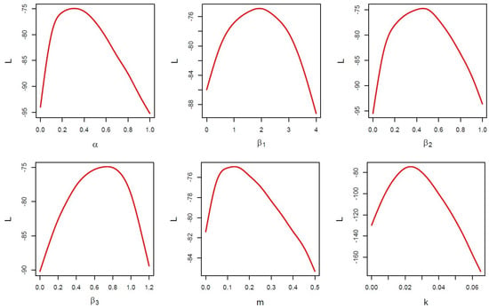
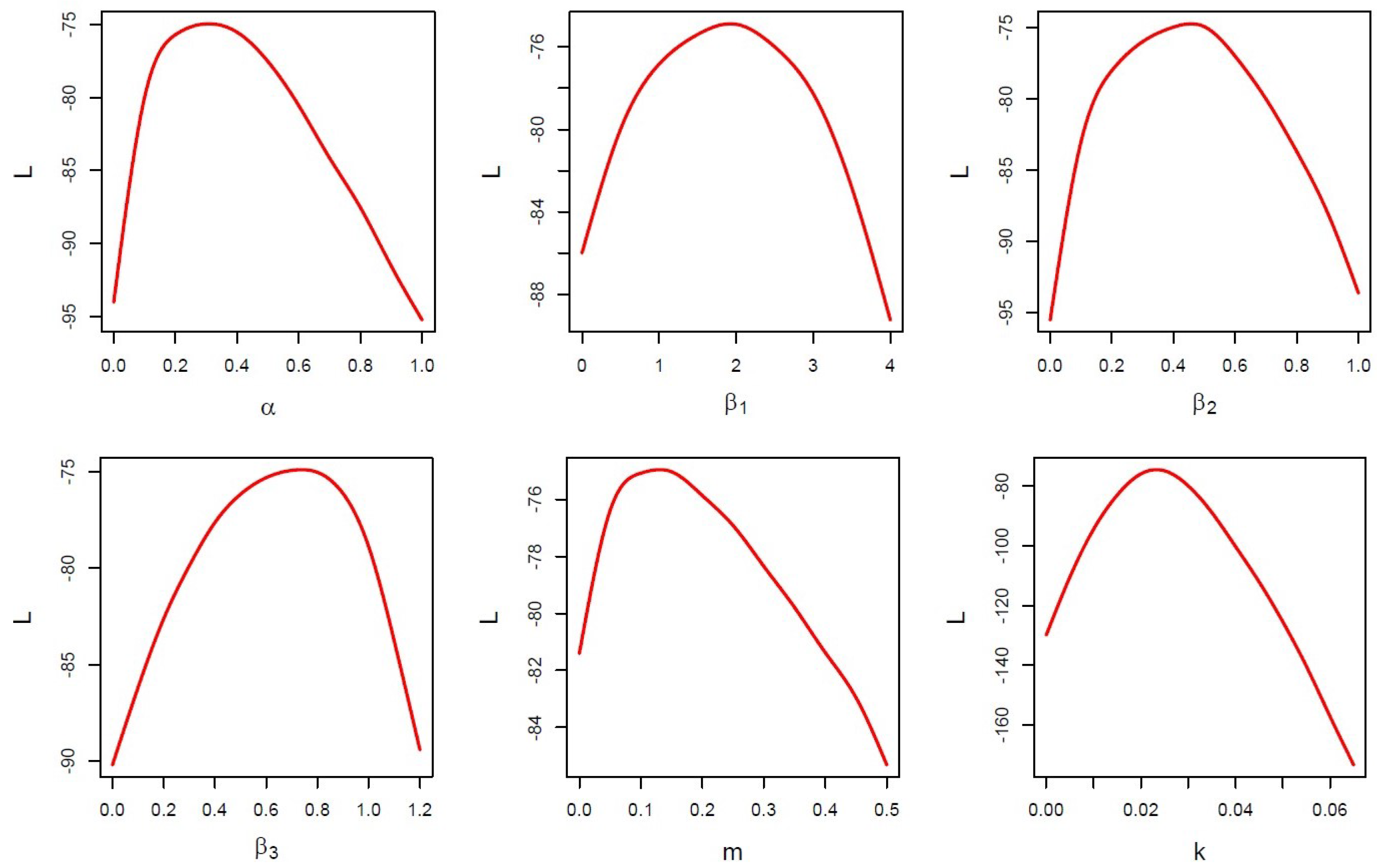
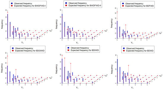
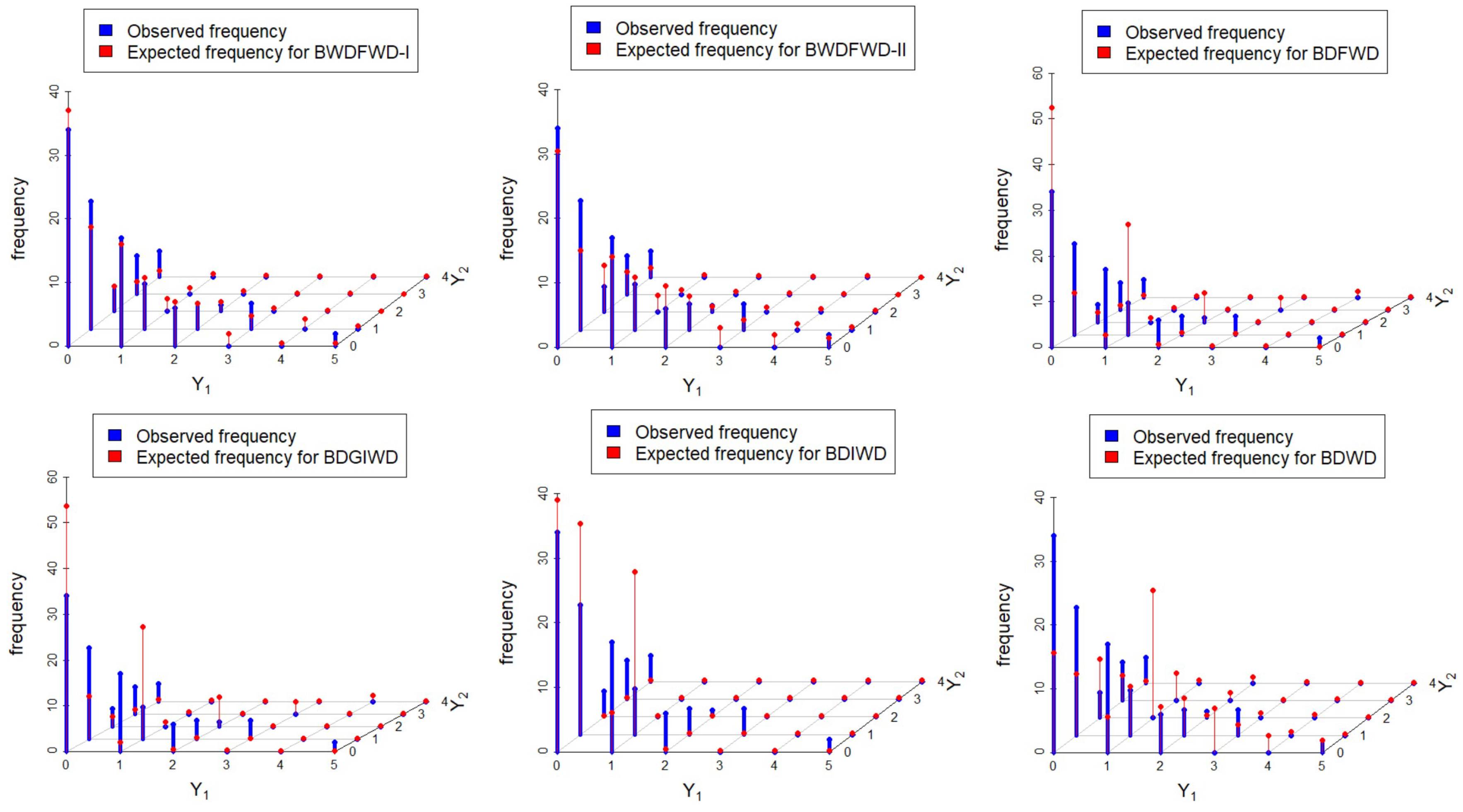
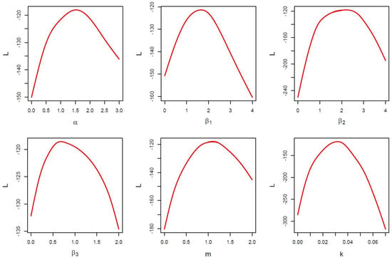
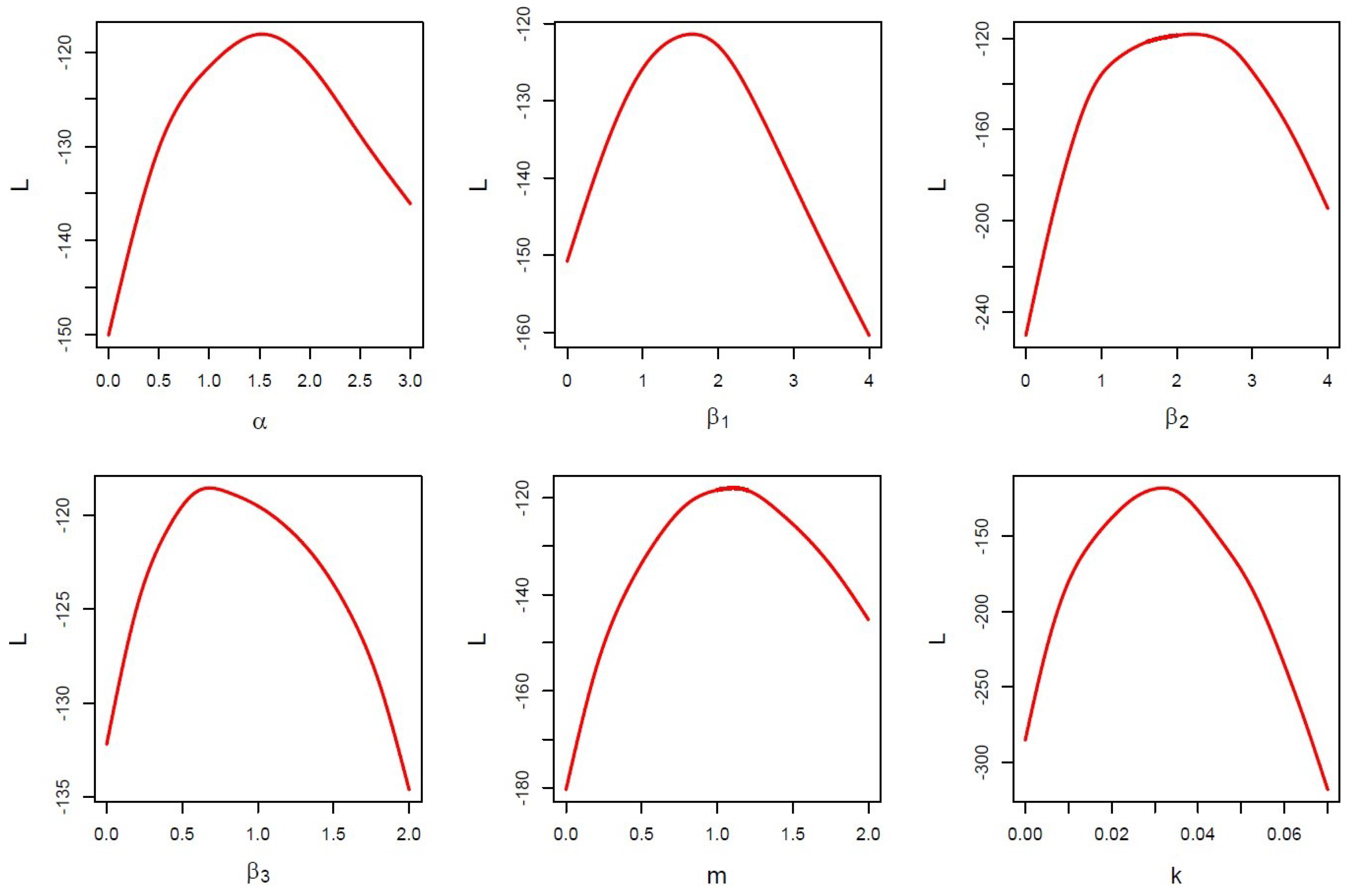
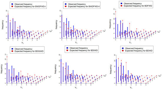
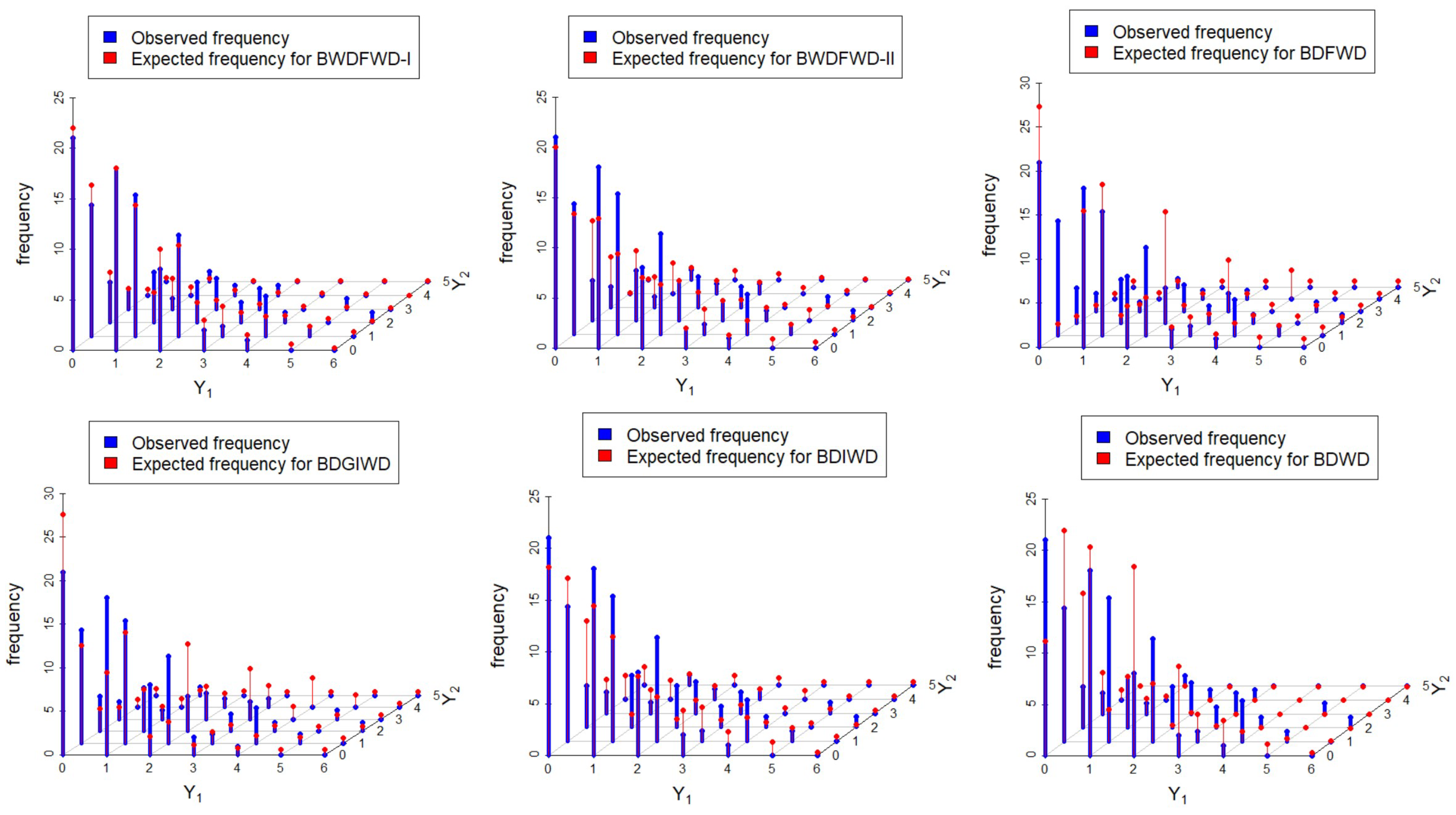
From Table 7, it can be observed that for dataset I, the values of the -log likelihood, AIC, BIC, and CAIC are comparatively the lowest for both the BWDFW-I and BWDFW-II models. However, the lowest values for the BWDFW-I model suggest that it provides the best fit for dataset I. Figure 7 shows the profiles of the L functions for BWDFW-I, which indicate that the estimators are unique. In Figure 8, the estimated joint frequency distributions for the BWDFW-I and BWDFW-II models, along with the BDFW, BDGIW, BDIW, and BDW distributions, are shown. The graphical representation clearly indicates that the BWDFW-I model fits dataset I the best.

Figure 7. The profiles of the L functions obtained using dataset I.

Figure 8. The observed and estimated joint frequency distribution plots of dataset I.

8.2. Security and Safety Field: Dataset II

The second dataset is accident data from 122 experienced shunters, where random variables $Y_1$ and $Y_2$ respectively represent the numbers of accidents in 1937–1942 and 1943–1947 (see Zamani et al. [28]). The frequency distribution of bivariate dataset II is presented in Table 8, and the summary statistics for this dataset are presented in Table 9.

Table 8. Bivariate frequency distribution of dataset II.

	$Y_2$	0	1	2	3	4	≥5	Total
$Y_1$
0		21	13	4	2	0	0	40
1		18	14	5	1	0	1	39
2		8	10	4	3	1	0	26
3		2	1	2	2	1	0	8
4		1	4	1	0	0	0	6
5		0	1	0	1	0	0	2
6		0	0	1	0	0	0	1
Total		50	43	17	9	2	1	122

Table 9. Descriptive statistics for dataset II.

Median		Mean		Covariance	Pearson’s Correlation	Spearman’s Rho	Kendall’s Tau
$Y_1$	$Y_2$	$Y_1$	$Y_2$	Cov($Y_1$,$Y_2$)	Cor($Y_1$,$Y_2$)	$\rho (Y_1,Y_2)$	$\tau (Y_1,Y_2)$
1.00	1.00	1.2700	0.9754	1.36208	0.93013	0.91082	0.87229

From the summary values presented in Table 9, it is clear that $Y_1$ exhibits a left tail, while $Y_2$ shows a right tail. Moreover, for dataset II, the values of the Pearson’s correlation coefficient, Spearman’s rho $\left(\rho \right)$, and Kendall’s tau $\left(\tau \right)$ indicate a strong positive correlation between $Y_1$ and $Y_2$. Therefore, these data are appropriate for modeling using the BWDFW-I and BWDFW-II models.

In Table 10, the MLEs (SEs in parentheses), $95\%$ confidence intervals, −log l, AIC, BIC, and CAIC obtained using dataset II are presented for the BWDFW-I, BWDFW-II, BDFW, BDGIW, BDIW, and BDW distributions.

Table 10. The MLEs (SEs in parentheses), $95\%$ confidence intervals, −log l, AIC, BIC, and CAIC for dataset II.

Model	Estimate (SE)	$95\%$ CI	−log l	AIC	BIC	CAIC
BWDFW-I	$\widehat{\alpha }$ = 1.45323  (0.19872)	(1.0637, 1.8427)	118.0931	248.1862	258.6122	253.3992
	$\widehat{{\beta }_1}$ = 2.08623  (0.32629)	(1.4467, 2.7258)
	$\widehat{{\beta }_2}$ = 2.22495  (0.38345)	(1.4734, 2.9765)
	$\widehat{{\beta }_3}$ = 0.64388  (0.08354)	(0.4801, 0.8076)
	$\widehat{m}$ = 1.19231  (0.12209)	(0.9530, 1.4316)
	$\widehat{k}$ = 0.03662  (0.00561)	(0.0256, 0.0476)
BWDFW-II	$\widehat{\alpha }$ = 0.21199  (0.03842)	(0.1367, 0.2873)	123.6967	259.3934	269.8194	264.6064
	$\widehat{{\beta }_1}$ = 1.61515  (0.38433)	(0.8619, 2.3684)
	$\widehat{{\beta }_2}$ = 1.25150  (0.29413)	(0.6750, 1.8280)
	$\widehat{{\beta }_3}$ = 1.23137  (0.18540)	(0.8680, 1.5948)
	$\widehat{m}$ = 1.04923  (0.22088)	(0.6163, 1.4822)
	$\widehat{k}$ = 0.11366  (0.04613)	(0.0232, 0.2041)
BDFW	$\widehat{{\theta }_1}$ = 0.53722  (0.05599)	(0.4275, 0.6470)	304.4232	616.8464	623.7971	620.3218
	$\widehat{{\theta }_2}$ = 0.96836  (0.03091)	(0.9078, 1.0289)
	$\widehat{{\theta }_3}$ = 0.42012  (0.04545)	(0.3310, 0.5092)
	$\widehat{\lambda }$ = 1.78756  (0.15202)	(1.4896, 2.0855)
BDGIW	$\widehat{q_1}$ = 0.73722  (0.08495)	(0.5707, 0.9037)	324.4139	656.8277	663.7784	660.3031
	$\widehat{q_2}$ = 0.68359  (0.01927)	(0.6458, 0.7214)
	$\widehat{q_3}$ = 0.44223  (0.03147)	(0.3805, 0.5039)
	$\widehat{\alpha }$ = 1.55918  (0.12410)	(1.3159, 1.8024)
BDIW	$\widehat{{\alpha }_1}$ = 0.61985 (0.07761)	(0.4677, 0.7720)	335.704	679.408	686.3587	682.8833
	$\widehat{{\alpha }_2}$ = 0.80355  (0.09387)	(0.6196, 0.9875)
	$\widehat{{\alpha }_3}$ = 0.17942  (0.02531)	(0.1298, 0.2290)
	$\widehat{\beta }$ = 1.61787  (0.18622)	(1.2529, 1.9829)
BDW	$\widehat{p_1}$ = 0.68978 (0.03364)	(0.6238, 0.7557)	367.2133	742.4266	749.3772	745.9019
	$\widehat{p_2}$ = 0.57694  (0.04008)	(0.4984, 0.6555)
	$\widehat{p_3}$ = 0.43879  (0.07138)	(0.2989, 0.5787)
	$\widehat{\alpha }$ = 1.47306  (0.09988)	(1.2773, 1.6688)

Dataset II best fits the suggested BWDFW-I model, as shown in Table 10, where the values of the -log likelihood, AIC, BIC, and CAIC are the lowest for BWDFWD Model 1. Figure 9 shows the profiles of the L functions for BWDFW-I. Furthermore, Figure 10 presents the estimated joint frequency distributions for the BWDFW-I, BWDFW-II, BDFW, BDGIW, BDIW, and BDW distributions. The graphical representation also clearly shows that dataset II is best fitted by the BWDFW-I model.

Figure 9. The profiles of the L functions obtained using dataset II.

Figure 10. The observed and estimated joint frequency distribution plots of dataset II.

9. Summary of the Key Findings

In this article, we proposed a bivariate extension of the weighted discretized Fréchet–Weibull distribution (WDFWD) using two different methods of operators. The first method involved taking the minimum of the two baseline random variables, resulting in what we called the BWDFW-I model. The second method, on the other hand, considered the maximum of the two baseline random variables and was referred to as the BWDFW-II model. Statistical properties, including the joint probability mass function, joint hazard rate, and joint reversed hazard rate functions, were presented for both distributions. The graphs illustrated that both the BWDFW-I and BWDFW-II models exhibited long right and left tails. Additionally, the various shapes of the joint hazard rate functions demonstrated their flexibility. The proposed models could also be applied to discuss dispersion data under various shapes of kurtosis. The joint probability-generating function was derived to obtain different moments and product moments. Positive quadrant dependence was proven. The simulation indicated that the MLE could be effectively used in the estimation process. To demonstrate the practical applicability of the two proposed models, we analyzed two real-life bivariate datasets (from the security and safety field and the aviation field) and compared them to four other discrete bivariate versions of the Weibull and extended Weibull distributions, namely, BDW, BDIW, BDGIW, and BDFW. It is widely acknowledged that augmenting the number of parameters enhances the distribution’s flexibility. Moreover, weighted distribution theory offers a valuable framework for comprehending distributions and contributes to their increased adaptability. The newly introduced bivariate weighted discretized Fréchet–Weibull distribution, which extends the weighted DFWD in a bivariate manner and incorporates six parameters, clearly exhibits greater flexibility than the four other distributions under consideration. Both BWDFW-I and BWDFW-II showed superior performances, yielding the lowest values for AIC, BIC, and CAIC. Furthermore, it was noted that the BWDFW-I model outperformed the BWDFW-II model, as the former exhibited lower values compared to the latter.

10. Future Directions

Bivariate distributions play a crucial role in modeling complex relationships between paired data across various disciplines, offering extensive practical applications. In this context, the BWDFW-I and BWDFW-II models provide a novel framework that can be effectively applied to real-world bivariate datasets. These models have the potential to yield a better fit compared to existing discrete bivariate distributions, making them valuable tools for analyzing dependent data structures in diverse fields.

To enhance the utility and robustness of these models, future research will focus on developing and implementing various parameter estimation techniques. Specifically, different algorithms, including the Expectation–Maximization (EM) algorithm, will be explored to optimize parameter estimation for datasets exhibiting complex dependency structures. Additionally, alternative estimation approaches tailored to different data types and distributions will be investigated to improve the accuracy and efficiency of statistical inferences.

Several existing studies have demonstrated the effectiveness of such algorithms in similar contexts. For instance, the EM algorithm has been successfully applied in a multivariate Student-t process model to analyze dependent tail-weighted degradation data (see Xu et al. [29]). This study highlights the advantages of the EM algorithm in handling complex multivariate structures with heavy tails, making it a promising method for extending the BWDFW models.

Furthermore, stress–strength reliability models have been widely used in reliability analysis, particularly in evaluating system performance under stress conditions. A notable example is the bivariate iterated Farlie–Gumbel–Morgenstern stress–strength reliability model developed for Rayleigh-distributed margins (see Chandra et al. [30]). This model provides valuable insights into the reliability properties of dependent systems, reinforcing the importance of adopting advanced estimation techniques for bivariate models.

Building on these advancements, future research will not only refine the estimation techniques for BWDFW models but also extend their applicability to a broader range of real-life bivariate datasets. This will include exploring hybrid approaches that integrate Bayesian and frequentist methods, leveraging computational techniques, such as Markov Chain Monte Carlo simulations, and assessing the performances of these models under different censoring schemes. By addressing these research directions, the proposed models will contribute significantly to the advancement of discrete bivariate modeling, offering practical solutions for real-world data analysis and decision making.

References

- Teamah, A.-E.A.M.; Elbanna, A.; Ahmed, M. Fréchet-Weibull distribution with application to earthquakes data sets. Pak. J. Stat. 2020, 36, 135–147. [Google Scholar]
- Alzaatreh, A.; Lee, C.; Famoye, F. A new method for generating families of continuous distributions. Metron 2013, 71, 63–79. [Google Scholar] [CrossRef] [Scilit]
- Das, D.; Das, B. Discretized Fréchet–Weibull distribution: Properties and application. J. Indian Soc. Probab. Stat. 2023, 24, 243–282. [Google Scholar] [CrossRef] [Scilit]
- Das, D.; Das, B. On weighted discretized Fréchet–Weibull distribution with application to real life data. Appl. Math. Inf. Sci. Int. J. 2023, 7, 791–806. [Google Scholar]
- Johnson, N.L.; Kotz, S.; Balakrishnan, N. Discrete Multivariate Distributions; Wiley: Hoboken, NJ, USA, 1997. [Google Scholar]
- Balakrishnan, N.; Lai, C. Continuous Bivariate Distributions, 2nd ed.; Springer: Berlin/Heidelberg, Germany, 2009. [Google Scholar]
- Kundu, D.; Gupta, R.D. Bivariate generalized exponential distribution. J. Multivar. Anal. 2009, 100, 581–593. [Google Scholar] [CrossRef] [Scilit]
- Sarhan, A.; Hamilton, D.C.; Smith, B.; Kundu, D. The bivariate generalized linear failure rate distribution and its multivariate extension. Comput. Stat. Data Anal. 2011, 55, 644–654. [Google Scholar] [CrossRef] [Scilit]
- El-Sherpieny, E.A.; Ibrahim, S.A.; Bedar, R.E. A new bivariate distribution with generalized Gompertz marginals. Asian J. Appl. Sci. 2013, 1, 141–150. [Google Scholar]
- Wagner, B.S.; Artur, J.L. Bivariate Kumaraswamy distribution: Properties and a new method to generate bivariate classes. Statistics 2013, 47, 1321–1342. [Google Scholar]
- Balakrishnan, N.; Shiji, K. On a class of bivariate exponential distributions. Stat. Probab. Lett. 2014, 85, 153–160. [Google Scholar] [CrossRef] [Scilit]
- El-Gohary, A.; El-Bassiouny, A.H.; El-Morshedy, M. Bivariate exponentiated modified Weibull extension distribution. J. Appl. Probab. Stat. 2016, 5, 67–78. [Google Scholar] [CrossRef] [Scilit]
- Hiba, Z.M. Bivariate inverse Weibull distribution. J. Stat. Comput. Simul. 2016, 86, 2335–2345. [Google Scholar]
- Rasool, R.; Akbar, A.J. On bivariate exponentiated extended Weibull family of distributions. Ciência Nat. 2016, 38, 564–576. [Google Scholar]
- Eliwa, M.; El-Morshedy, M. Bivariate odd Weibull-G family of distributions: Properties, Bayesian and non-Bayesian estimation with bootstrap confidence intervals and application. J. Taibah Univ. Sci. 2020, 14, 331–345. [Google Scholar] [CrossRef] [Scilit]
- Kocherlakota, S.; Kocherlakota, K. Bivariate Discrete Distributions; Marcel Dekker: New York, NY, USA, 1992. [Google Scholar]
- Basu, A.P.; Dhar, S.K. Bivariate geometric distribution. J. Appl. Stat. Sci. 1995, 2, 33–44. [Google Scholar]
- Kumar, C.S. A unified approach to bivariate discrete distributions. Metrika 2008, 67, 113–123. [Google Scholar] [CrossRef] [Scilit]
- Kemp, A.W. New discrete Appell and Humbert distributions with relevance to bivariate accident data. J. Multivar. Anal. 2013, 113, 2–6. [Google Scholar] [CrossRef] [Scilit]
- Lee, H.; Cha, J.H. On two general classes of discrete bivariate distributions. Am. Stat. 2015, 69, 221–230. [Google Scholar] [CrossRef] [Scilit]
- Nekoukhou, V.; Kundu, D. Bivariate discrete generalized exponential distribution. Statistics 2017, 51, 1143–1158. [Google Scholar] [CrossRef] [Scilit]
- El-Morshedy, M.; Eliwa, M.S.; Gohary, A.E.; Khalil, A.A. Bivariate exponentiated discrete Weibull distribution: Statistical properties, estimation, simulation and applications. Math. Sci. 2020, 14, 29–42. [Google Scholar] [CrossRef] [Scilit]
- Ali, S.; Shafqat, M.; Shah, I.; Dey, S. Bivariate discrete Nadarajah and Haghighi distribution: Properties and different methods of estimation. Filomat 2019, 33, 5589–5610. [Google Scholar] [CrossRef] [Scilit]
- Kundu, D.; Nekoukhou, V. On bivariate discrete Weibull distribution. Commun. Stat.—Theory Methods 2019, 48, 3464–3481. [Google Scholar] [CrossRef] [Scilit]
- Shibu, D.S.; Beegum, N. Bivariate Discrete Modified Weibull (BDMW) Distribution. Statistica 2021, 81, 231–264. [Google Scholar]
- Barbiero, A. Discrete analogues of continuous bivariate probability distributions. Ann. Oper. Res. 2022, 312, 23–43. [Google Scholar] [CrossRef] [Scilit]
- Mitchell, C.R.; Paulson, A.S. A new bivariate negative binomial distribution. Nav. Res. Logist. Q. 1981, 28, 359–374. [Google Scholar] [CrossRef] [Scilit]
- Zamani, H.; Faroughi, P.; Ismail, N. Bivariate Poisson-weighted exponential distribution with applications. AIP Conf. Proc. 2014, 1602, 964–968. [Google Scholar]
- Xu, A.; Fang, G.; Zhuang, L.; Gu, C. A multivariate student-t process model for dependent tail-weighted degradation data. IISE Trans. 2024, 1–17. [Google Scholar] [CrossRef] [Scilit]
- Chandra, N.; James, A.; Domma, F.; Rehman, H. Bivariate iterated Farlie–Gumbel–Morgenstern stress–strength reliability model for Rayleigh margins: Properties and estimation. Stat. Theory Relat. Field 2024, 8, 315–334. [Google Scholar] [CrossRef] [Scilit]
Disclaimer/Publisher’s Note: The statements, opinions and data contained in all publications are solely those of the individual author(s) and contributor(s) and not of MDPI and/or the editor(s). MDPI and/or the editor(s) disclaim responsibility for any injury to people or property resulting from any ideas, methods, instructions or products referred to in the content. |
© 2025 by the authors. Licensee MDPI, Basel, Switzerland. This article is an open access article distributed under the terms and conditions of the Creative Commons Attribution (CC BY) license (https://creativecommons.org/licenses/by/4.0/).