Analysing Disease Spread on Complex Networks Using Forman–Ricci Curvature

Abstract

Infectious-disease dynamics depend on heterogeneous contact structure, which classical homogeneous-mixing models such as SIR/SEIR cannot capture. We develop a curvature-informed network SIR framework that embeds Forman–Ricci curvature (FRC), a discrete topological descriptor of fragility and robustness, into per-edge transmission. We compute FRC on undirected and directed Erdős–Rényi, Watts–Strogatz, Barabási–Albert, and Power–Law Cluster networks, and relate curvature to degree, clustering, and betweenness to identify structurally influential nodes and bridge edges. Using curvature-adjusted transmission, we simulate epidemics across topologies and infection rates, then validate predictively with a controlled “hidden-truth” benchmark: posterior-calibrated FRC models are compared with advanced centrality-weighted baselines (EdgeBetweenness, Degree, Eigenvector) under identical fit/holdout splits. On heterogeneous graphs (Barabási–Albert/Power–Law Cluster), FRC improves holdout Root Mean Squared Error (RMSE), peak-time accuracy, and final-size proximity. A compact sensitivity analysis over baseline transmission and clustering, with Partial Rank Correlation Coefficient (PRCC), shows these gains are robust across parameter regimes. Intervention ablations (cases averted vs. budget) further show that vaccinating high-curvature nodes and protecting extreme negative-curvature bridges can outperform EdgeBetweenness targeting at practical budgets. Directed networks exhibit sharper peaks and faster resolution, with strongly negative out-curvature marking putative exporters. In general, FRC provides a principled geometric signal that enhances network epidemic models and yields concrete, topology-aware guidance for targeted vaccination and community-bridge control.

1. Introduction

Network theory has become a pivotal framework in epidemiology, offering profound insight into the patterns and dynamics of disease spread in human populations [1,2,3,4]. The essence of applying network theory in this field lies in its ability to model complex interactions between individuals as nodes connected by edges [5,6], representing potential paths for pathogen transmission [7,8,9]. This approach contrasts markedly with traditional compartmental models such as SIR that often assume homogeneous mixing within populations [10,11,12], thus missing critical structural nuances that can significantly influence infection outcomes. In particular, early network-based SIR analyses established how heterogeneity reshapes epidemic thresholds and prevalence [13], while more recent COVID-19 modelling has demonstrated how age structure, human mobility, and non-pharmaceutical interventions interact over networked populations [14].

The integration of network theory into epidemiological modelling can provide a more granular perspective by considering variations in individual contact patterns, which can vary widely on social, spatial, and temporal scales [15]. For example, scale-free networks, characterized by their heavy-tailed degree distributions, highlight the presence of super-spreaders, that is, individuals linked to an exceptionally high number of contacts, thus disproportionately affecting the spread of diseases [16]. In contrast, small-world networks, known for their high clustering coefficient and short average path lengths [17], exemplify how tightly knit community structures can rapidly spread an infection locally while maintaining the potential for rapid global transmission through occasional long-range connections. Beyond pairwise contacts, higher-order (group-level) interactions on simplicial and hypergraph structures can substantially alter contagion pathways and critical points; recent reviews systematize these effects and provide unified formalisms for epidemic processes on higher-order networks [18].

Erdős–Rényi networks, which can be generated by connecting nodes randomly with a fixed probability [19], offer a baseline for studying epidemic dynamics in homogeneous populations. These types of networks lack the hierarchical structure of the hubs, resulting in relatively uniform connectivity. As such, they are valuable for exploring epidemic spread in systems where all individuals are equally likely to interact.

On the other hand, power-law cluster networks combine the scale-free property of heavy-tailed degree distributions with high local clustering, simulating the structure of tightly knit communities with influential hubs [20]. This dual property of power-law cluster networks makes them particularly relevant for understanding disease dynamics in close-contact settings, where local clusters can amplify infections, while hubs facilitate rapid spread across broader networks.

By modelling these complex interaction patterns, network theory allows epidemiologists to more accurately predict which nodes (i.e., individuals or groups) are at the highest risk of infection, identify potential outbreak sources, and evaluate the efficacy of intervention strategies designed to disrupt pathogenic pathways [21]. In parallel, concepts of robustness and resilience from network science clarify how heterogeneous connectivity concentrates vulnerabilities and informs targeted dismantling or immunization schemes, insights that dovetail with epidemic control [22].

The Forman–Ricci curvature, adapted from its original mathematical context by Robin Forman, is a topological measure used to assess the “robustness” or “fragility” of interactions within a network [23]. In the setting of network theory, curvature is used to quantify how well-connected a network is around a particular node or along an edge. Networks with positive curvature are typically dense and well-connected [24], indicating that nodes mutually reinforce each other’s connectivity, which can lead to rapid spread of disease within these clusters. Conversely, areas of negative curvature suggest bottlenecks or weak links in the network, which can act as potential barriers to disease transmission.

Incorporating curvature into epidemiological models provides a nuanced view of disease dynamics, highlighting potential areas where interventions could be most effective. For instance, targeting nodes or edges with high positive curvature for vaccination or quarantine measures could theoretically disrupt the spread more efficiently than strategies that do not consider network topology.

Despite the promising applications of curvature in network analysis [25], a significant gap exists in the literature regarding its use in epidemiology-specific network models. Both undirected and directed networks are vital for modelling infectious diseases. Undirected networks often represent symmetric interactions, such as household or community contact networks, while directed networks capture inherently directional interactions, such as sexual contacts, vector-borne transmission, or transmission in transportation networks. However, to the best of our knowledge, studies that directly incorporate Forman–Ricci curvature into mathematical epidemiological models have not yet been carried out. In particular, directed networks have not received sufficient attention in epidemiology despite their importance in understanding asymmetric interactions. Existing studies on epidemics in networks largely focus on undirected models and overlook how the directionality of edges might influence the implications of curvature on disease spread [26,27,28].

Thus, empirical studies correlating the Forman–Ricci curvature with disease outcomes in mathematical epidemiology modelling have not been conducted. This gap is especially evident in complex networks, where the nature of edge connections can significantly alter the network’s topology and, therefore, its epidemiological behaviour.

In this research, we develop a curvature-modulated network SIR framework that embeds Forman–Ricci curvature directly into the per-edge transmission rate and systematically evaluate its epidemiological consequences, outbreak timing, and final size, across Erdős–Rényi (ER), Watts–Strogatz (WS), Barabási–Albert (BA), and Power-Law Cluster (PLC) networks, including directed variants. To establish practical relevance, we calibrate and validate curvature-weighted dynamics against other network comparators (EdgeBetweenness, Degree, Eigenvector, and a uniform network SIR) and conduct compact sensitivity and robustness analyses over baseline transmission rate (${\beta }_0$) and clustering controls. The resulting curvature-informed rules yield concrete strategies for prioritizing hubs and protecting bridge edges in real settings.

The rest of this paper is structured as follows: the Materials and Methods are described and formulated in Section 2. In Section 3, the Validation and Simulation studies are presented, and in Section 4, we conclude with a summary and discussion, highlighting key findings and potential directions for future research.

2. Materials and Methods

2.1. Networks Generation and Modeling

The development of network models for this study involves the construction of networks that capture distinct topological properties, including scale-free, small-world, random graph, and power-law cluster networks. Each of these models is used to provide unique insights into the dynamics of infectious disease transmission within networks and their implications for public health interventions.

2.1.1. Scale-Free Networks

Scale-free networks exhibit a power-law degree distribution, where a few highly connected nodes, or hubs, dominate. These networks, generated by the Barabási–Albert (BA) model, use preferential attachment, where new nodes are more likely to connect to existing high-degree nodes. The degree distribution follows:

$$P\left(k\right)\propto k^{-\zeta }$$

(1)

where $\zeta$ typically ranges from 2 to 3. Scale-free networks are robust to random failures but highly vulnerable to targeted attacks on hubs, making them crucial for studying super-spreader events in epidemics.

2.1.2. Small-World Networks

Small-world networks combine high clustering coefficients with short path lengths. The Watts–Strogatz (WS) model generates these networks by rewiring edges in a regular lattice with probability p, introducing shortcuts that significantly reduce path lengths. The model is given by

$$L\left(p\right)\approx {\displaystyle \frac{logN}{log(⟨k⟩p)}}$$

(2)

where $L\left(p\right)$ is the average path length; N, the number of nodes; and $⟨k⟩$, the average degree. These properties facilitate the rapid transmission of diseases, providing insight into epidemic dynamics.

2.1.3. Erdős–Rényi Networks (Random Graphs)

The Erdős–Rényi (ER) model creates random graphs by connecting n nodes with probability p. The degree distribution follows a Poisson distribution:

$$P\left(k\right)={\displaystyle \frac{{\lambda }^k{e}^{-\lambda }}{k!}}$$

(3)

where $\lambda =⟨k⟩$ is the mean degree. ER networks lack hubs, resulting in homogeneous connectivity. Their simplicity makes them ideal for modelling baseline epidemic dynamics in non-hierarchical networks.

2.1.4. Power-Law Cluster Networks

The Power-Law Cluster (PLC) model builds on the Barabási–Albert model by incorporating a clustering probability p, encouraging triangular connections. This creates networks with a power-law degree distribution and high clustering coefficients, mirroring real-world network structures. The clustering probability that governs triangle formation is given by

$$P\left(\mathrm{triangle}\right)\propto p$$

(4)

where p balances preferential attachment with local clustering. PLC networks are particularly effective for studying disease spread in close-knit communities.

2.2. Curvature Calculation

2.2.1. Forman–Ricci Curvature for Undirected and Directed Networks

Forman–Ricci curvature extends the concept of Ricci curvature to both undirected and directed networks, mathematically represented as $G=(V,E)$, where V is the set of nodes (vertices) and E is the set of edges connecting the nodes. The curvature provides a measure of robustness and structural significance, which varies depending on the local topology of the graph and the weights assigned to its edges.

For an undirected network, the Forman–Ricci curvature for an edge e connecting nodes $v_1$ and $v_2$ is given by the following equation:

$$F\left(e\right)=w_e\left({\displaystyle \frac{w_{v1}}{w_e}}+{\displaystyle \frac{w_{v2}}{w_e}}-\sum _{e_{v1}\sim e}{\displaystyle \frac{w_{v1}}{\sqrt{w_e{w}_{e_{v1}}}}}-\sum _{e_{v2}\sim e}{\displaystyle \frac{w_{v2}}{\sqrt{w_e{w}_{e_{v2}}}}}\right)$$

(5)

where $w_e>0$ denotes the weight of edge e, and $w_{v1},w_{v2}>0$ are the weights of the incident nodes $v_1$ and $v_2$. The notation $e_{v1}\sim e$ denotes the set of undirected edges incident to $v_1$ other than e (i.e., edges sharing node $v_1$ with e, excluding e itself), and similarly, $e_{v2}\sim e$ denotes the set of undirected edges incident to $v_2$ other than e. For each adjacent edge in these sets, $w_{e_{v1}}$ and $w_{e_{v2}}$ are the corresponding edge weights. (When the graph is unweighted, all node and edge weights are set to one.) In the unweighted case, this reduces to the canonical expression

$$F\left(e\right)=4-deg\left(v_1\right)-deg\left(v_2\right),$$

since each sum counts $deg\left(v_i\right)-1$ adjacent edges at endpoint $v_i$. This formulation provides insights into network robustness and identifies structurally significant regions [25]. This equation takes into account the neighboring edge weights and node weights to provide a comprehensive evaluation of local connectivity and resilience.

For a directed network, the Forman–Ricci curvature for an edge e from node $v_1$ to node $v_2$ is computed using the following equation:

$$F\left(e\right)=w_e\left({\displaystyle \frac{w_{v1}}{w_e}}-\sum _{e_{v1}\sim e}{\displaystyle \frac{w_{v1}}{\sqrt{w_e{w}_{e_{v1}}}}}\right)+w_e\left({\displaystyle \frac{w_{v2}}{w_e}}-\sum _{e_{v2}\sim e}{\displaystyle \frac{w_{v2}}{\sqrt{w_e{w}_{e_{v2}}}}}\right)$$

(6)

where $e=(v_1\to v_2)$ is a directed edge, $w_e>0$ denotes the weight of edge e, and $w_{v1},w_{v2}>0$ are the weights of incident nodes $v_1$ and $v_2$. The notation $e_{v1}\sim e$ denotes the set of outgoing edges from $v_1$ other than e (i.e., edges $v_1\to x$ with $x\ne v_2$), while $e_{v2}\sim e$ denotes the set of incoming edges incident to $v_2$ other than e (i.e., edges $x\to v_2$ with $x\ne v_1$); for each such adjacent edge, $w_{e_{v1}}$ and $w_{e_{v2}}$ are the corresponding edge weights. Factors $\sqrt{w_e{w}_{e_{v1}}}$ and $\sqrt{w_e{w}_{e_{v2}}}$ normalize contributions with the geometric mean of the interacting edge weights, following the standard directed Forman–Ricci construction [29,30]. In unweighted graphs (in which all node and edge weights equal are to one), Equation (6) reduces to

$$F\left(e\right)=4-\mathrm{outdeg}\left(v_1\right)-\mathrm{indeg}\left(v_2\right),$$

where $\mathrm{outdeg}\left(v_1\right)$ and $\mathrm{indeg}\left(v_2\right)$ are the out- and in-degrees of $v_1$ and $v_2$, respectively. This formulation incorporates both node and edge weights and adapts to the asymmetry introduced by edge directions, making it highly relevant for analyzing directed networks.

The summation terms account for the edges adjacent to the nodes connected by the edge e. If we denote the set of incoming and outgoing edges for node v by $E_{I,v}$ and $E_{O,v}$, then the in-Forman curvature $F_I\left(v\right)$ and out-Forman curvature $F_O\left(v\right)$ are given as follows:

$$F_I\left(v\right)=\sum _{e\in E_{I,v}}F\left(e\right)$$

(7)

$$F_O\left(v\right)=\sum _{e\in E_{O,v}}F\left(e\right)$$

(8)

Here, the summations are taken over only the incoming and outgoing edges, respectively. Hence, the total amount of flow through node v is given as

$$F_{I/O}\left(v\right)=F_I\left(v\right)-F_O\left(v\right)$$

(9)

The formulation for directed networks accounts for the asymmetry introduced by edge directions, making it suitable for networks where directionality plays a significant role.

2.2.2. Algorithm Development

We implemented the above formulae of the Forman–Ricci curvature (FRC) in both undirected and directed networks using Python (version 3.12.11) with the NetworkX library. The computation process involves iterating over all edges in the network, calculating curvature values based on node and edge weights, and accounting for directionality, in the case of directed networks. The algorithms are detailed below.

Algorithm 1 computes the Forman–Ricci curvature for undirected networks by iterating through each edge $e=(u,v)$ in the graph $G=(V,E)$. It calculates the curvature $F\left(e\right)$ based on the edge weights, node weights, and the contributions from adjacent edges. The resulting curvature provides insights into the structural robustness and connectivity properties of the network.

Algorithm 1 FRC for Undirected Networks

Require:  Undirected graph $G=(V,E)$ with node weights $\{w_v>0\}$ and edge weights $\{w_e>0\}$ (default $w_{·}=1$) Ensure:  Edge curvatures $F_e$ for all $e\in E$; node curvatures $F_v^{\mathrm{sum}}$ and (optional) $F_v^{\mathrm{avg}}$ for all $v\in V$  1: Initialize $F_v^{\mathrm{sum}}\Leftarrow 0$ for all $v\in V$  2: for each undirected edge $e=\{u,v\}\in E$ do  3:     $w_e\Leftarrow$ weight of edge $\{u,v\}$;   $w_u\Leftarrow$ weight of node u;   $w_v\Leftarrow$ weight of node v  4:     ${\mathrm{sum}}_u\Leftarrow 0$;   ${\mathrm{sum}}_v\Leftarrow 0$  5:     for each neighbor x of u with edge $\{u,x\}\in E$, $x\ne v$ do    ▹ edges incident to u excluding e  6:         $w_{ux}\Leftarrow$ weight of edge $\{u,x\}$  7:         ${\mathrm{sum}}_u\Leftarrow {\mathrm{sum}}_u+{\displaystyle \frac{w_u}{\sqrt{w_e{w}_{ux}}}}$  8:     for each neighbor y of v with edge $\{v,y\}\in E$, $y\ne u$ do    ▹ edges incident to v excluding e  9:          $w_{vy}\Leftarrow$ weight of edge $\{v,y\}$  10:         ${\mathrm{sum}}_v\Leftarrow {\mathrm{sum}}_v+{\displaystyle \frac{w_v}{\sqrt{w_e{w}_{vy}}}}$  11:     $F_{\{u,v\}}\Leftarrow w_e\left({\displaystyle \frac{w_u}{w_e}}+{\displaystyle \frac{w_v}{w_e}}-{\mathrm{sum}}_u-{\mathrm{sum}}_v\right)$  12:     Assign $F_{\{u,v\}}$ to edge $\{u,v\}$  13:     $F_u^{\mathrm{sum}}\Leftarrow F_u^{\mathrm{sum}}+F_{\{u,v\}}$;   $F_v^{\mathrm{sum}}\Leftarrow F_v^{\mathrm{sum}}+F_{\{u,v\}}$  14: Optional: for any $v\in V$ with degree $deg\left(v\right)>0$, set $F_v^{\mathrm{avg}}\Leftarrow {\displaystyle \frac{F_v^{\mathrm{sum}}}{deg\left(v\right)}}$  ▹ average node curvature

Algorithm 2 computes the Forman–Ricci curvature for directed networks by iterating through each directed edge $e=(u,v)$ in the graph $G=(V,E)$. The calculation incorporates the contributions from incoming edges to node u and outgoing edges from node v. By considering edge weights, node weights, and directionality, the algorithm quantifies the structural robustness and flow characteristics of the network.

Algorithm 2 FRC for Directed Networks

Require:  Directed graph $G=(V,E)$ with node weights $\{w_v>0\}$ and edge weights $\{w_e>0\}$ (default $w_{·}=1$) Ensure:  Edge curvatures $F_e$ for all $e\in E$; node curvatures $F_v^{\mathrm{out}}$, $F_v^{\mathrm{in}}$ for all $v\in V$  1: Initialize $F_v^{\mathrm{out}}\Leftarrow 0$ and $F_v^{\mathrm{in}}\Leftarrow 0$ for all $v\in V$  2: for each directed edge $(u,v)\in E$ do  3:     $w_e\Leftarrow$ weight of edge $(u,v)$; $w_u\Leftarrow$ weight of node u; $w_v\Leftarrow$ weight of node v  4:     ${\mathrm{sum}}_u^{\mathrm{out}}\Leftarrow 0$,   ${\mathrm{sum}}_v^{\mathrm{in}}\Leftarrow 0$  5:     for each outgoing neighbor x of u with edge $(u,x)\in E$, $x\ne v$ do  6:         $w_{ux}\Leftarrow$ weight of edge $(u,x)$  7:         ${\mathrm{sum}}_u^{\mathrm{out}}\Leftarrow {\mathrm{sum}}_u^{\mathrm{out}}+{\displaystyle \frac{w_u}{\sqrt{w_e{w}_{ux}}}}$  8:     for each incoming neighbor x of v with edge $(x,v)\in E$, $x\ne u$ do  9:          $w_{xv}\Leftarrow$ weight of edge $(x,v)$  10:         ${\mathrm{sum}}_v^{\mathrm{in}}\Leftarrow {\mathrm{sum}}_v^{\mathrm{in}}+{\displaystyle \frac{w_v}{\sqrt{w_e{w}_{xv}}}}$  11:     $F_{(u,v)}\Leftarrow w_e\left({\displaystyle \frac{w_u}{w_e}}-{\mathrm{sum}}_u^{\mathrm{out}}\right)+w_e\left({\displaystyle \frac{w_v}{w_e}}-{\mathrm{sum}}_v^{\mathrm{in}}\right)$  12:     Assign $F_{(u,v)}$ to edge $(u,v)$  13:     $F_u^{\mathrm{out}}\Leftarrow F_u^{\mathrm{out}}+F_{(u,v)}$      ▹ node out-curvature (sum over outgoing edges)  14:     $F_v^{\mathrm{in}}\Leftarrow F_v^{\mathrm{in}}+F_{(u,v)}$          ▹ node in-curvature (sum over incoming edges)  15: Optional: define $F_v^{\mathrm{avg}}\Leftarrow {\displaystyle \frac{F_v^{\mathrm{out}}+F_v^{\mathrm{in}}}{\mathrm{outdeg}\left(v\right)+\mathrm{indeg}\left(v\right)}}$ for reporting a single node score

2.3. Integration of Disease Spread Models with FRC

Classical mathematical epidemiological models such as the SIR (Susceptible–Infectious–Recovered) model offer a foundational framework for studying disease dynamics under the assumption of a homogeneously mixed population. In this classical setting, every individual is assumed to interact equally with every other individual, leading to the following system of ordinary differential equations:

$$\left\{\begin{array}{c}{\displaystyle \frac{dS}{dt}}=-\beta SI,\hfill \\ {\displaystyle \frac{dI}{dt}}=\beta SI-\gamma I,\hfill \\ {\displaystyle \frac{dR}{dt}}=\gamma I\hfill \end{array}\right.$$

(10)

Here, $S\left(t\right),I\left(t\right),$ and $R\left(t\right)$ denote the proportions of susceptible, infected, and recovered individuals at time t; $\beta$ is the transmission rate; and $\gamma$ is the recovery rate.

However, in real-world settings, populations are not well mixed. Individuals interact through structured, heterogeneous social or physical contact patterns. This motivates a shift from classical compartmental models to network-based SIR formulations, where the population is represented by a graph $G=(V,E)$. Each node $i\in V$ denotes an individual and each edge $(i,j)\in E$, a potential contact through which infection may spread. Every node carries compartmental state variables $(S_i\left(t\right)$, $I_i\left(t\right)$, and $R_i\left(t\right)$, interpreted as the local probability (or proportion) of being susceptible, infected, or recovered, respectively, and the local conservation condition holds:

$$S_i\left(t\right)+I_i\left(t\right)+R_i\left(t\right)=1,\forall i\in V.$$

We propose a curvature-modulated network SIR model in which the per-edge transmission rate is a deterministic function of the Forman–Ricci curvature (FRC). Specifically, as a defining component of our framework, we set

$${\beta }_{ij}:={\beta }_{0}exp\left[F\left(e\right)\right],e=(i,j)(\mathrm{for}\mathrm{directed}\mathrm{networks}e=i\to j),$$

where ${\beta }_0$ is a baseline transmission rate, and $F\left(e\right)$ is the FRC of edge e. This mapping ensures ${\beta }_{ij}>0$ and makes transmission endogenously reflect local network geometry. Throughout, we use robust in the FRC sense of being locally well-supported: edges embedded in neighborhoods with many short alternative paths (e.g., triangles/squares; high local transitivity) have larger $F\left(e\right)$ and hence larger ${\beta }_{ij}$, favoring rapid within-community spread. Conversely, edges that act as bridges between sparsely connected regions (tree-like surroundings with few two-step alternatives) have smaller $F\left(e\right)$ and therefore smaller ${\beta }_{ij}$, reflecting topology-induced fragility and throttling inter-community transmission.

Many sparse networks naturally yield predominantly negative-edge FRC because most edges are not reinforced by redundant short cycles. Crucially, $F\left(e\right)<0$ does not mean most nodes are globally “not robust”: FRC is an edge-level descriptor, and a node can be incident to both positive and negative edges; its in-/out-curvature may therefore take either sign. Edges with $F\left(e\right)<0$ often act as bridges between communities, which is epidemiologically influential for long-range seeding yet structurally fragile, since removing them disrupts connectivity more than removing edges embedded in redundant motifs. In our model, $F\left(e\right)>0$ up-weights ${\beta }_{ij}$ on locally reinforced edges (promoting within-community spread), whereas $F\left(e\right)<0$ down-weights ${\beta }_{ij}$ on bridge-like edges; the exponential mapping attenuates, but does not eliminate, transmission on negative-FRC edges.

Thus, the dynamics of the proposed system are governed by the following set of differential equations for each node $i\in V$:

$$\begin{array}{cc}\hfill {\displaystyle \frac{d{S}_i}{dt}}& =-\sum _{j\in N\left(i\right)}{\beta }_{ij}{S}_i{I}_j\hfill \end{array}$$

(11)

$$\begin{array}{cc}\hfill {\displaystyle \frac{d{I}_i}{dt}}& =\sum _{j\in N\left(i\right)}{\beta }_{ij}{S}_i{I}_j-\gamma I_i\hfill \end{array}$$

(12)

$$\begin{array}{cc}\hfill {\displaystyle \frac{d{R}_i}{dt}}& =\gamma I_i\hfill \end{array}$$

(13)

Here, $\gamma$ is the recovery rate, assumed uniform across all nodes, and it captures how infected individuals transition to the recovered state. $N\left(i\right)$ is the neighborhood of node i, defined as $N\left(i\right)=\{j\mid (i,j)\in E\}.$ In the case of directed networks, we refine the notion of neighborhood into in-neighborhood $\left(N_{\mathrm{in}}\left(i\right)=\{j\mid (j,i)\in E\}\right)$, and out-neighborhood $\left(N_{\mathrm{out}}\left(i\right)=\{j\mid (i,j)\in E\}\right)$. This distinction allows the model to capture directionality in contact, e.g., where the disease may be transmitted from j to i, but not vice versa. Neighborhood $N\left(i\right)$ defines the local connectivity of each node i, determining potential sources and targets of infection. This modified SIR model, enriched with curvature-dependent dynamics, provides a refined tool for studying epidemic propagation in realistic and structured populations. This bridges geometric and epidemiological perspectives by linking transmission dynamics to the underlying network geometry, making it particularly useful for modeling diseases in complex systems with heterogeneous interaction patterns. We present the detailed mathematical properties and analysis of the proposed model in Appendix A.

2.4. Advanced Baselines and Calibration

To isolate the added value of curvature, we benchmark the FRC-weighted kernel against three other network models that weight transmission with established centrality measures. For every undirected graph $G=(V,E)$, we compute an edge feature $z_e$ and form the contact matrix

$${\beta }_{ij}:={\beta }_{0}exp\left(\alpha {\tilde{z}}_{ij}\right),{\tilde{z}}_{ij}={\displaystyle \frac{z_{ij}-{\mu }_z}{{\sigma }_z}},$$

with $\alpha =1$ and feature standardization $({\mu }_z,{\sigma }_z)$ taken over the edges. The four models are the following: (i) FRC: undirected Forman–Ricci curvature on edges; (ii) EdgeBetweenness: standard edge betweenness centrality; (iii) Eigenvector: sum of node eigenvector centralities $(x_i+x_j)$ on each edge; (iv) Degree: log product of degrees $log\left\{(d_i+\epsilon )(d_j+\epsilon )\right\}$. Uniform weighting serves as a sanity check.

2.4.1. Hidden Truth and Seeds

For each topology (ER, WS, BA, PLC), we generate a “hidden truth” trajectory using FRC with ${\beta }_0^{★}=0.3$. Initial infections are placed on endpoints of negative-FRC bridges with a max–min spacing heuristic (six seeds), reflecting likely inter-community introductions.

2.4.2. Calibration and Validation

For each baseline, we calibrate ${\beta }_0$ using a random-walk Markov chain Monte Carlo (MCMC) scheme on $log{\beta }_0$ [31,32], using a weakly informative log-normal prior centered by an early-growth proxy (spectral fallback if needed). The likelihood is Gaussian on the mean infected fraction $\overline{I}\left(t\right)$ over the first $25\%$ of the trajectory (fit window); we report posterior means and $90\%$ credible bands and conduct the evaluation on the remaining $75\%$ (holdout).

2.4.3. Metrics

On the holdout, we compute RMSE for $\overline{I}\left(t\right)$, absolute peak time error $|\Delta t_{\mathrm{peak}}|$, and a final-size proxy $|\Delta R(\infty \left)\right|$ (area under $\overline{I}\left(t\right)$).

2.4.4. Link to Sensitivity Checks

The same calibration setup (fit on the first $25\%$ and evaluation on the holdout) is used in our sensitivity and robustness checks (Section 2.5). This analysis evaluates three kernels, FRC, EdgeBetweenness, and a Uniform (unweighted) network SIR baseline, while retaining the FRC hidden-truth generator and the seed placement rule described above. To enable exhaustive parameter sweeps, we replace MCMC with a deterministic one-dimensional line search for ${\beta }_0$ on the fit window; the holdout metrics remain unchanged.

2.5. Sensitivity and Robustness Analysis

We assess robustness across transmission and topology by sweeping the hidden-truth baseline rate ${\beta }_0\in [0.1,0.6]$ and the family-specific clustering knob: ER (edge probability p), WS (rewiring probability p), BA (attachment m), and PLC (triangle probability p). For each grid point, we (i) generate the hidden-truth trajectory with FRC-weighted transmission, (ii) place six seeds on the endpoints of negative-FRC bridges with max–min spacing, and (iii) recalibrate ${\beta }_0$ for each comparator kernel by minimizing fit-window MSE via golden-section search (same fit/holdout split as above).

On the holdout, we compute three errors for the mean infected curve $\overline{I}\left(t\right)$: RMSE, absolute peak time error $|\Delta t_{\mathrm{peak}}|$, and final-size error $|\Delta R(\infty \left)\right|$ (from the area under $\overline{I}\left(t\right)$). To isolate the curvature contribution, we report the following differences:

$$\begin{array}{cc}\hfill \Delta \mathrm{RMSE}& = \mathrm{RMSE}\left(\mathrm{baseline}\right)-\mathrm{RMSE}\left(\mathrm{FRC}\right),\hfill \\ \hfill \Delta |t_{\mathrm{peak}}|& = |t_{\mathrm{peak}}{|}_{\mathrm{baseline}}-{\left|t_{\mathrm{peak}}\right|}_{\mathrm{FRC}},\hfill \\ \hfill \Delta \left|R\right(\infty \left)\right|& = {\left|R(\infty )\right|}_{\mathrm{baseline}}-{\left|R(\infty )\right|}_{\mathrm{FRC}}.\hfill \end{array}$$

where positive values indicate that FRC performs better. We present $\Delta \mathrm{RMSE}$ heatmaps comparing EdgeBetweenness against FRC across the four network families, together with analogous $\Delta \left|R\right(\infty \left)\right|$ heatmaps computed on the same parameter grid (Uniform and additional panels are provided in the Supplementary Materials).

We quantify parameter influence on the accuracy gap using partial rank correlation coefficients (PRCCs) of $\Delta \mathrm{RMSE}$ with respect to ${\beta }_0$ while controlling for the clustering knob (${\beta }_0\mid p$) and vice versa ($p\mid {\beta }_0$). Aggregate win rates (percentage of grid cells with $\Delta >0$) and PRCCs. Across all families, FRC wins the vast majority of cells for RMSE, peak timing, and final size, with PRCC magnitudes indicating that gains are largest at lower ${\beta }_0$ and in regimes of stronger structural heterogeneity (e.g., small m in BA, moderate p in WS/PLC).

3. Validation and Simulation Studies

This section assembles empirical and predictive evidence for the curvature–epidemic link. First, we validate computed FRC on canonical network families (ER, WS, BA, PLC) by comparing empirical distributions with their expected structural signatures and by checking alignment with established descriptors, thereby confirming that FRC captures salient meso-scale organization in both undirected and directed settings.

Second, we assess predictive performance under the hidden-truth protocol of Section 2.4 and Section 2.5: outbreaks generated with an FRC-weighted kernel are contrasted with calibrated comparators (EdgeBetweenness, Degree, Eigenvector, and a Uniform network SIR). Using the same calibration/holdout setup and accuracy criteria specified in Section 2, we quantify the out-of-sample fit to isolate the incremental value of curvature.

Third, to probe robustness concisely, we vary the baseline transmission ${\beta }_0$ and each family’s clustering (or attachment) knob, summarizing effects with heatmaps of error differences (baseline minus FRC), partial rank correlations (PRCC) with respect to ${\beta }_0$ and clustering, and an aggregate win rate table. Finally, we translate these differences into operational terms via intervention ablations, reporting expected cases averted as a function of vaccination budget when targeting nodes by negative-FRC versus edge-betweenness. Together, these analyses connect curvature structure to epidemic dynamics and to concrete, budget-aware control strategies.

3.1. FRC Distributions in Undirected and Directed Networks

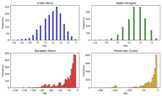
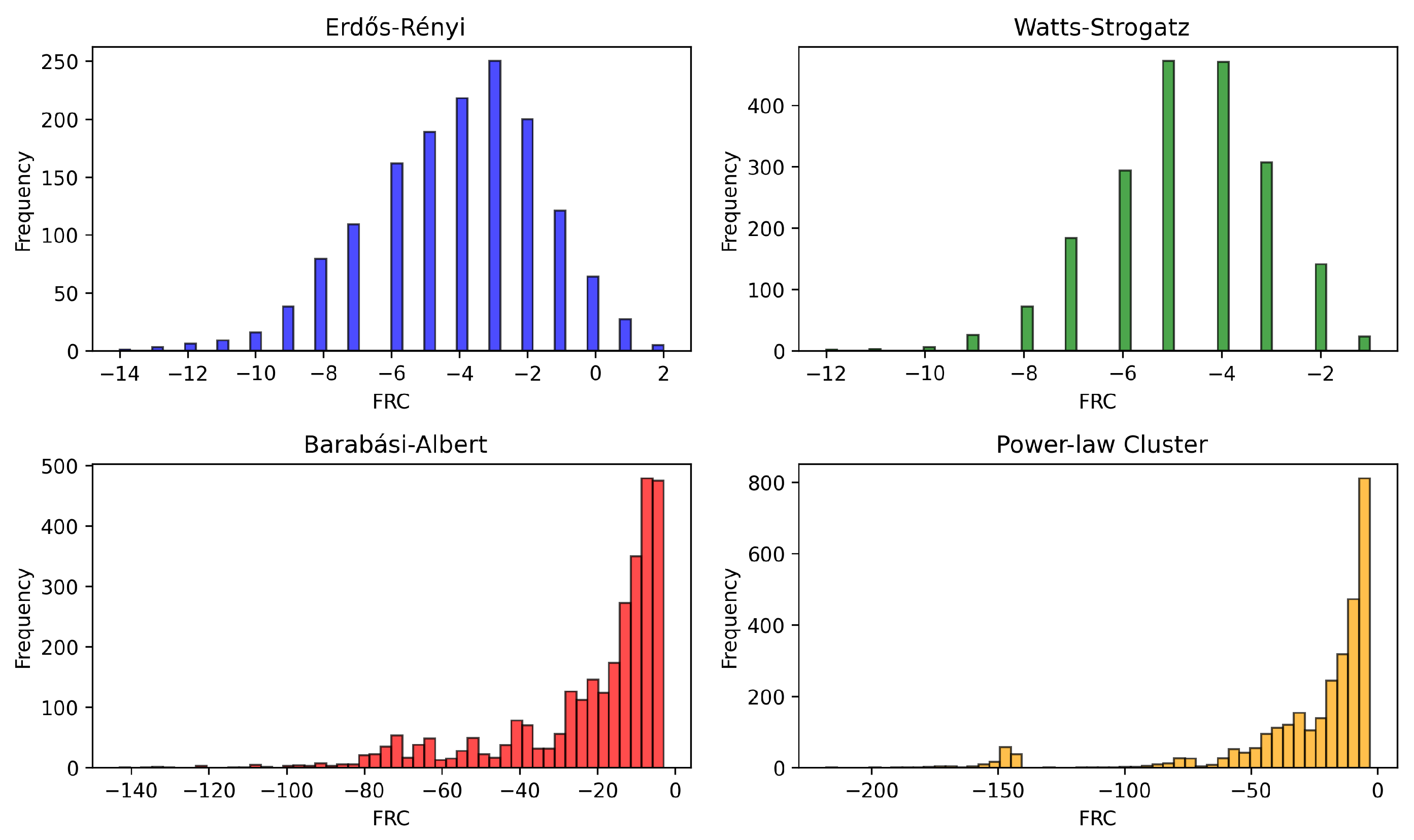
Figure 1 presents the FRC distributions for four undirected network models: Erdős–Rényi (1000 nodes, edge probability $p=0.003$), Watts–Strogatz (1000 nodes, mean degree $k=10$, rewiring probability $p=0.1$), Barabási–Albert (1000 nodes, $m=3$ edges per new node), and Power-Law Cluster (1000 nodes, $m=5$, and clustering probability $p=0.05$).

Figure 1. Distribution of undirected FRC across four undirected network models: Erdős–Rényi (ER), Watts–Strogatz (WS), Barabási–Albert (BA), and Power-Law Cluster (PLC).

These models demonstrate distinct structural characteristics reflected in their FRC distributions. The Erdős–Rényi model exhibits a symmetric distribution, reflecting its randomness, while the Watts–Strogatz model shows tighter clustering indicative of small-world properties. With their scale-free and clustered structures, the Barabási–Albert and Power-Law Cluster models display highly skewed FRC distributions dominated by negative curvature values, highlighting the prominence of hubs and clustering.

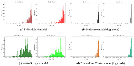
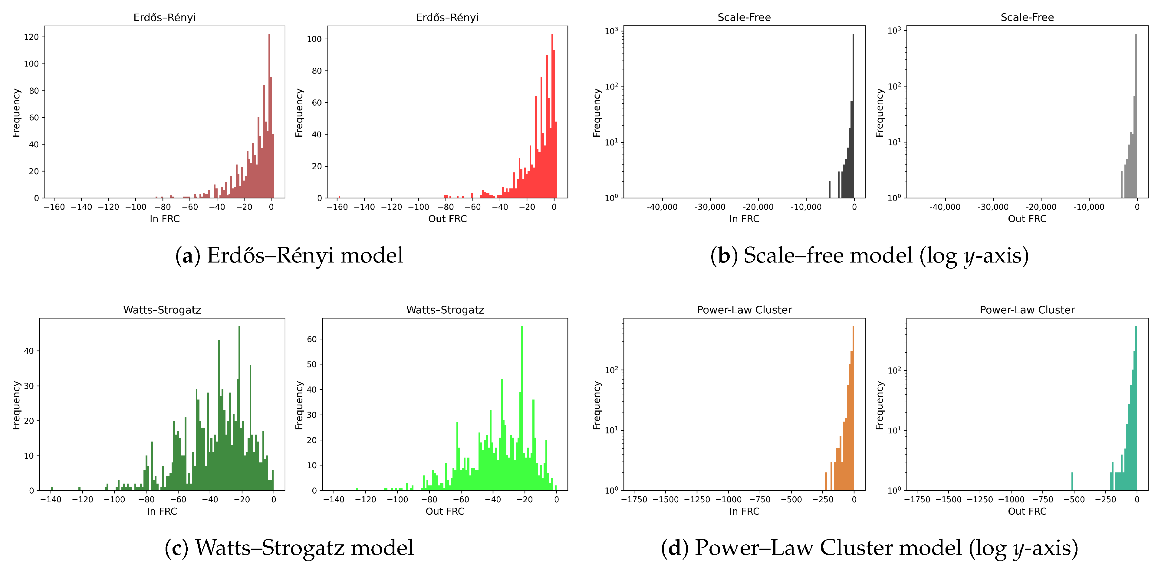
Figure 2 shows the distribution of in-degree and out-degree FRC for directed networks generated using four network models: the Erdős–Rényi model (1000 nodes, edge creation probability $p=0.003$), the scale-free model (1000 nodes, power-law degree exponents ${\lambda }_{in}={\lambda }_{out}=2.1$), the Watts–Strogatz model (1000 nodes, each connected to $k=10$ nearest neighbors, rewiring probability $p=0.1$), and the Power-Law Cluster model (1000 nodes, attachment parameter $m=3$, triangle formation probability $p=0.05$).

Figure 2. Distribution of directed Forman–Ricci curvature (FRC) across directed network models: (a) Erdős–Rényi model; (b) Scale–free model (logarithmic y-axis); (c) Watts–Strogatz model; (d) Power–Law cluster model (logarithmic y-axis). Panels (b,d) use a log scale on the y-axis to better highlight the heavy-tailed frequencies.

The Erdős–Rényi model shows near-zero, narrowly spread FRC, reflecting random, homogeneous connectivity. Scale–free networks (log (y)-axis) are strongly skewed with heavy negative tails, driven by hubs and many low-degree nodes. The Watts–Strogatz model exhibits moderate variability, consistent with small-world balance between clustering and shortcuts. Power–Law Cluster (log (y)-axis) is heavy-tailed with sharply negative values, reflecting hierarchical, transitive structure.

An extreme negative curvature marks edges and neighborhoods poorly supported by short alternative routes. Epidemiologically, such bridges are structurally fragile yet dynamically influential, enabling inter-community jumps. In directed graphs, very negative in-curvature identifies importers, very negative out-curvature identifies exporters, and both are bottlenecks for cross-community spread. Under ${\beta }_{ij}:={\beta }_0{e}^{F\left(e\right)}$, negative (F(e)) attenuates bridge transmission relative to cluster-internal edges, yet placement still yields outsized effects. This supports dual interventions: immunize hubs inside high-curvature clusters to curb local amplification, and protect or monitor extreme-negative-curvature bridges to reduce spillover.

3.2. Analysis of Correlation Between FRC and Measures of Centrality

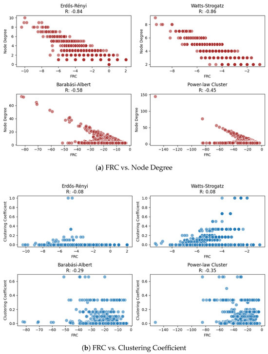
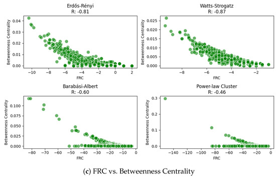
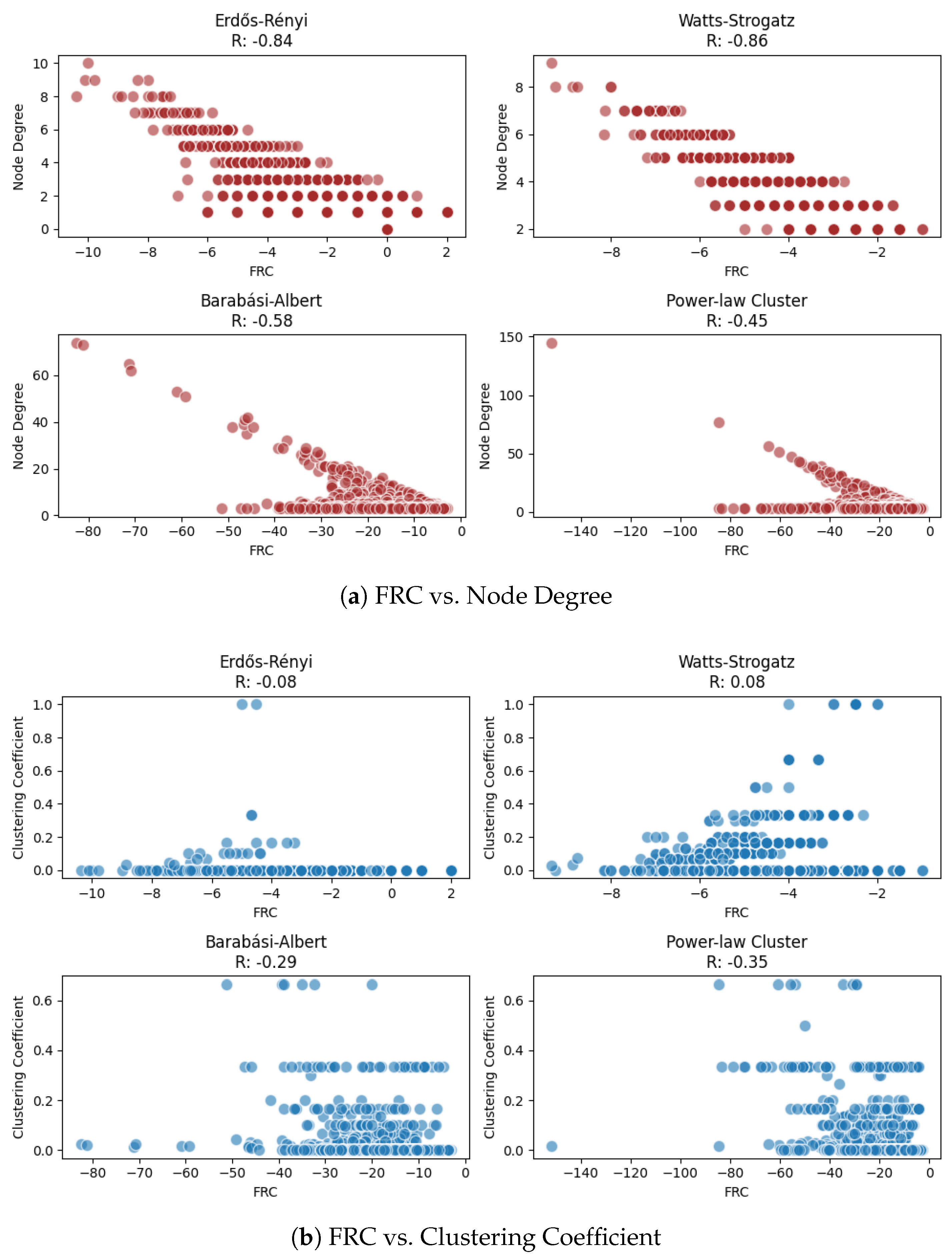
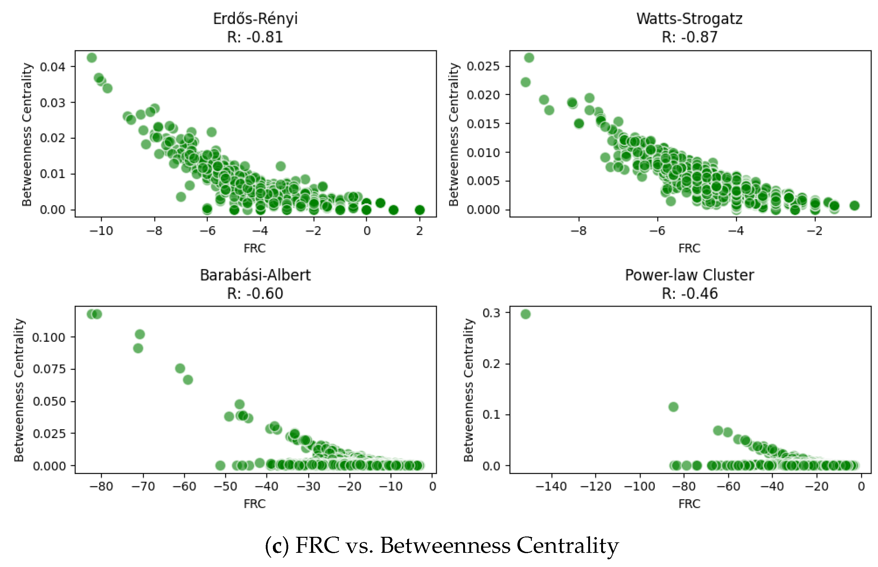
Figure 3 presents the relationship between FRC and three centrality measures, that is, node degree, clustering coefficient, and betweenness centrality, in undirected networks. Figure 3a reveals an inverse correlation, where nodes with higher curvature values tend to have lower degrees, indicating that less connected nodes often exhibit higher curvature. Figure 3b shows a weak positive relationship, suggesting that nodes involved in tightly knit communities exhibit slightly higher curvature. Lastly, Figure 3c highlights that nodes with higher betweenness centrality, critical for network flow, tend to have lower curvature values.

Figure 3. Correlation between Forman–Ricci curvature (FRC) and centrality measures in four undirected network models: Erdős–Rényi (ER), Watts–Strogatz (WS), Barabási–Albert (BA), and Power–Law Cluster (PLC). Rows correspond to network families; columns show (a) FRC vs. degree, (b) FRC vs. clustering coefficient, and (c) FRC vs. betweenness centrality.

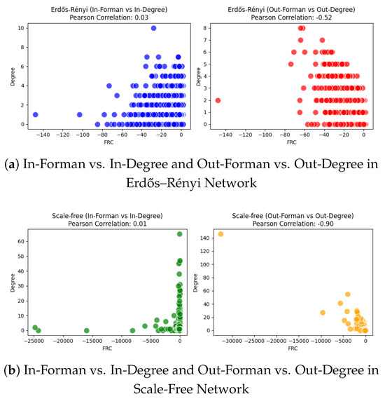
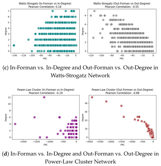
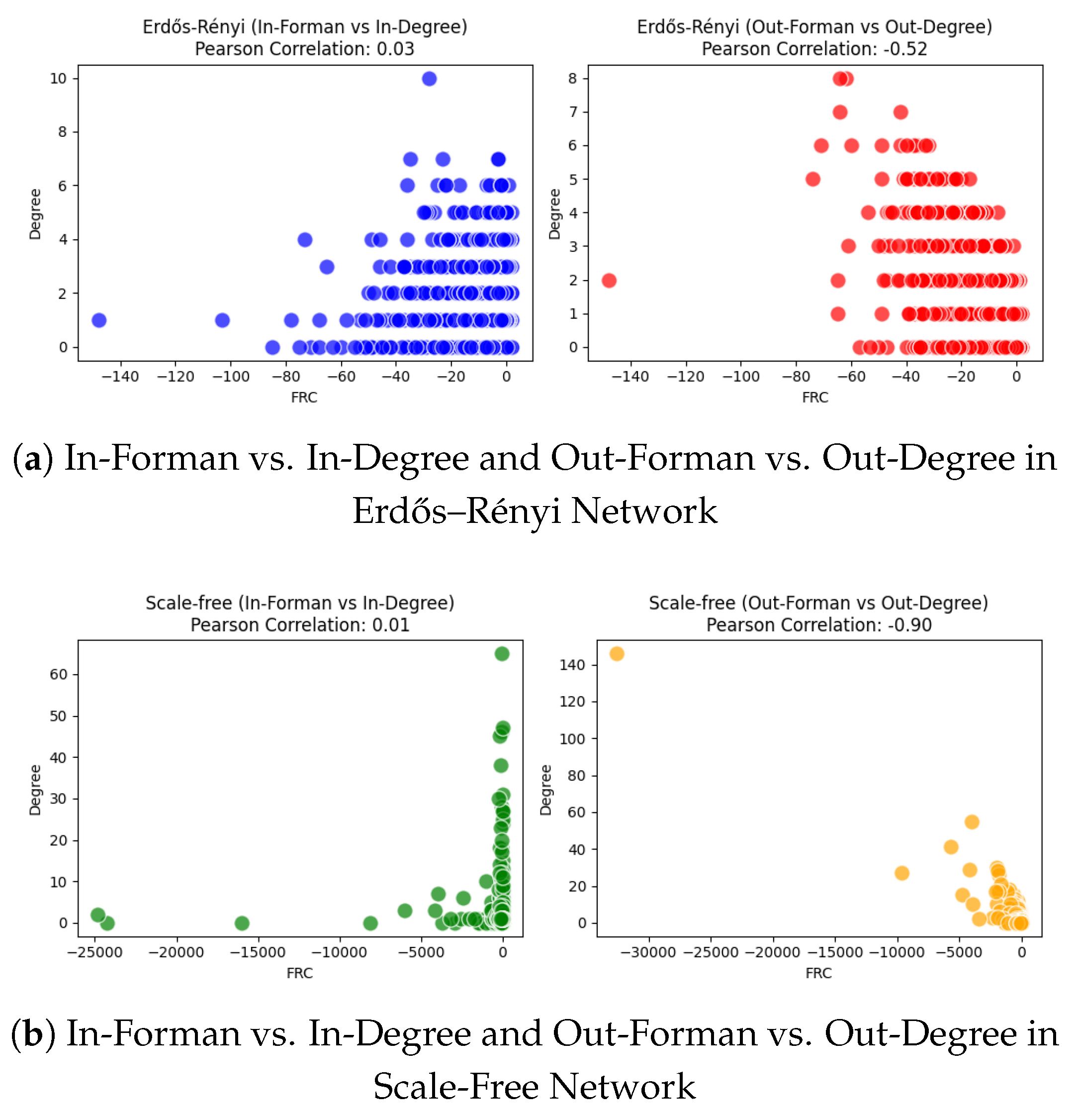
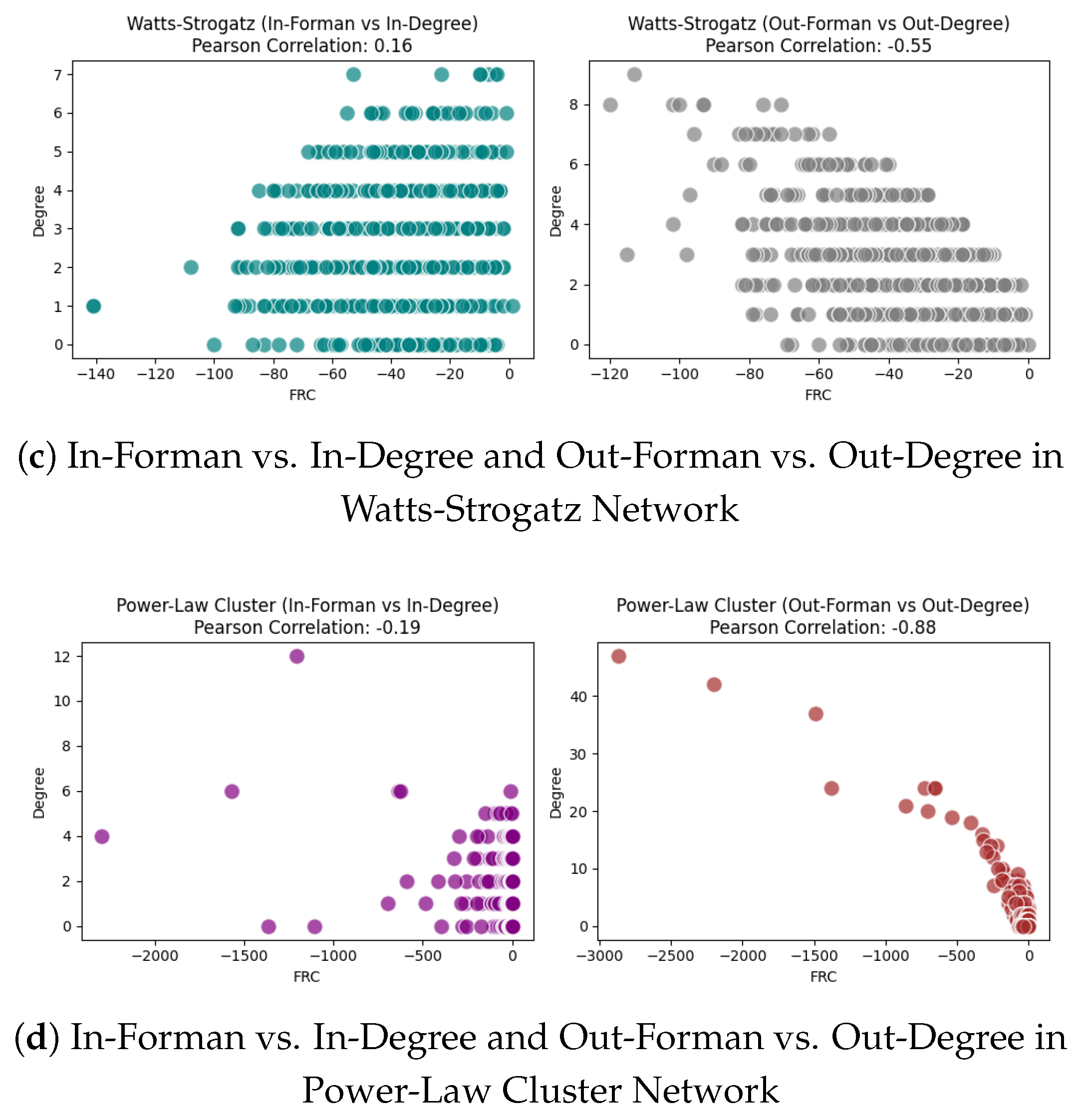
Figure 4 shows degree-curvature relationships in directed networks. Out-Forman curvature is consistently negatively correlated with out-degree and strongest in scale-free (r = $-0.90$), followed by Power-Law Cluster (r = $-0.88$), Watts-Strogatz (r = $-0.55$), and Erdős-Rényi (r = $-0.52$). Thus, high out-degree (potential super-spreader) nodes typically exhibit strongly negative curvature, indicating structural fragility and outsized influence. By contrast, correlations between in-Forman and in-degree are weak or negligible, evidencing directional asymmetry.

Figure 4. Correlation between directed Forman-Ricci curvature and degree across four directed network models. Panels: (a) Erdős–Rényi (ER), (b) scale-free (Barabási–Albert, BA), (c) Watts–Strogatz (WS), (d) Power–Law Cluster (PLC).

3.3. SIR Dynamics with Undirected Forman–Ricci Curvature

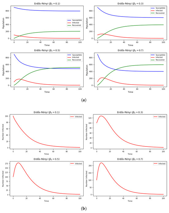
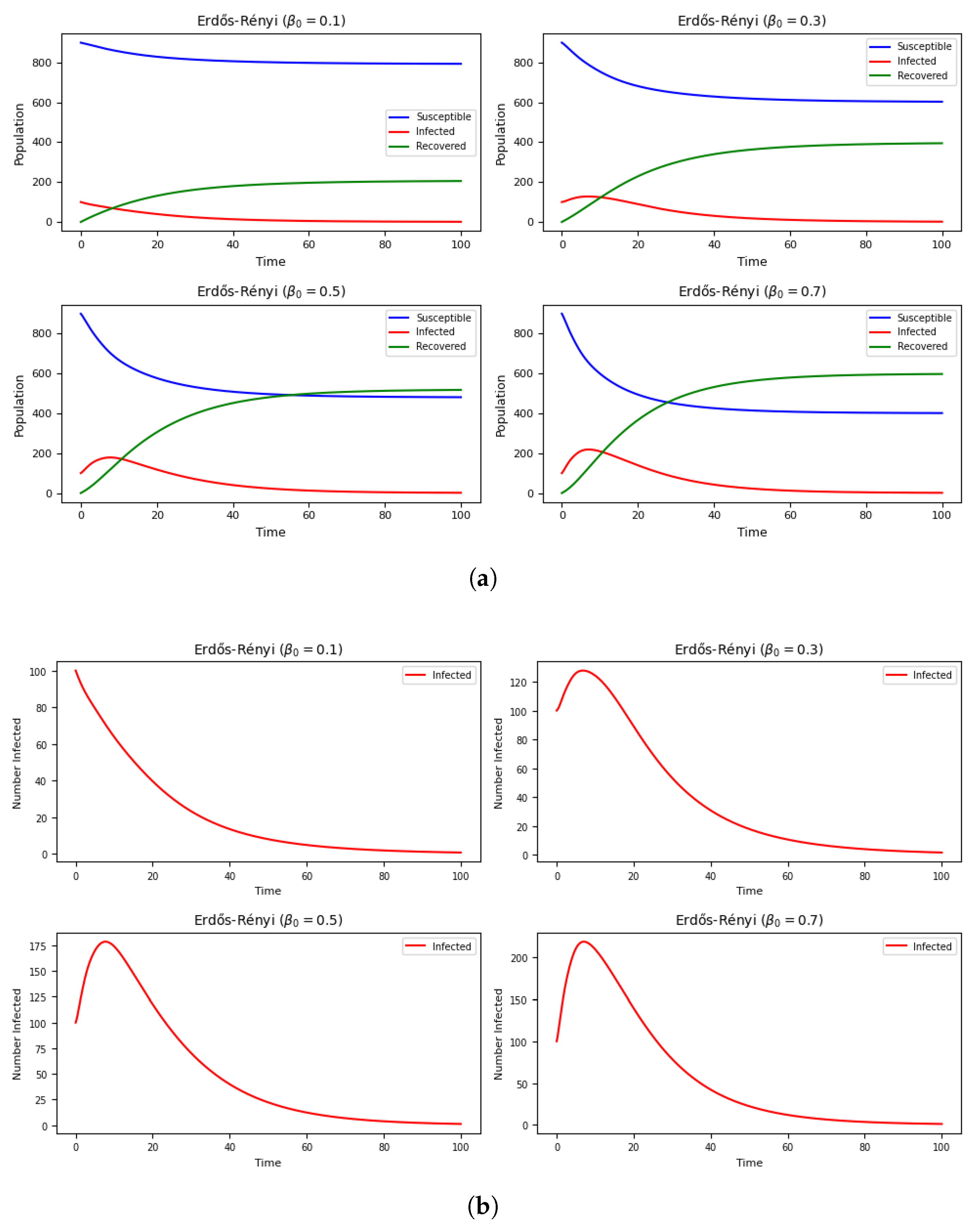
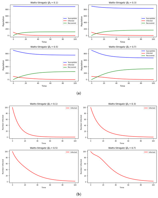
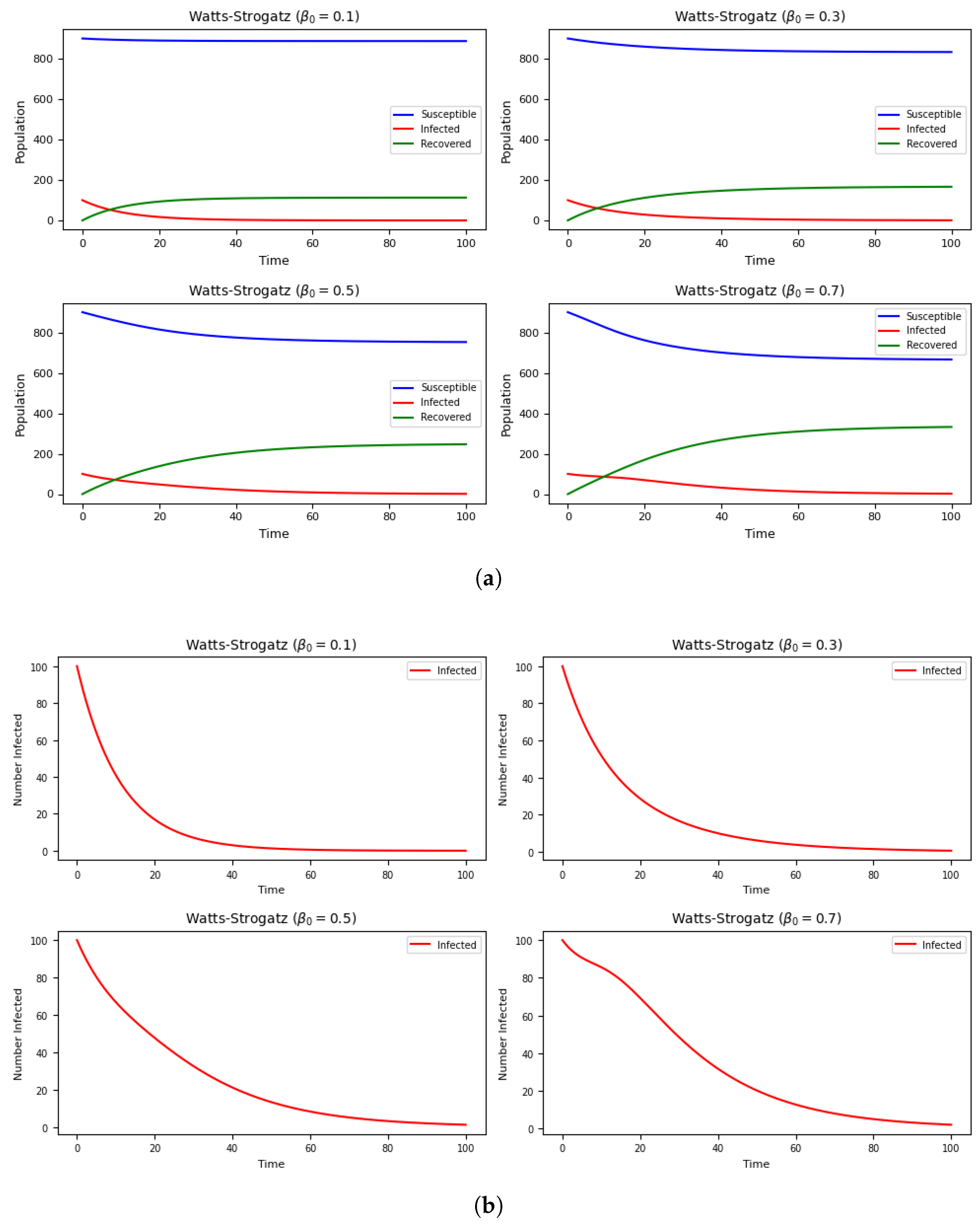
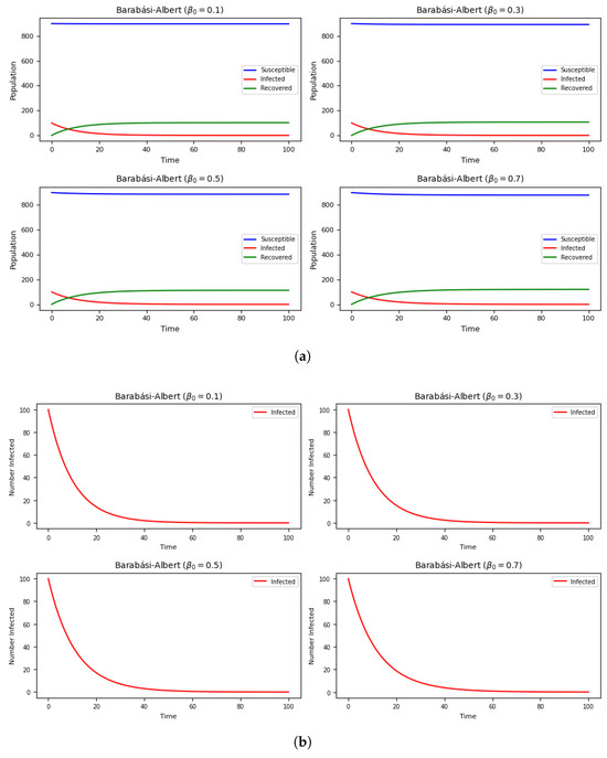
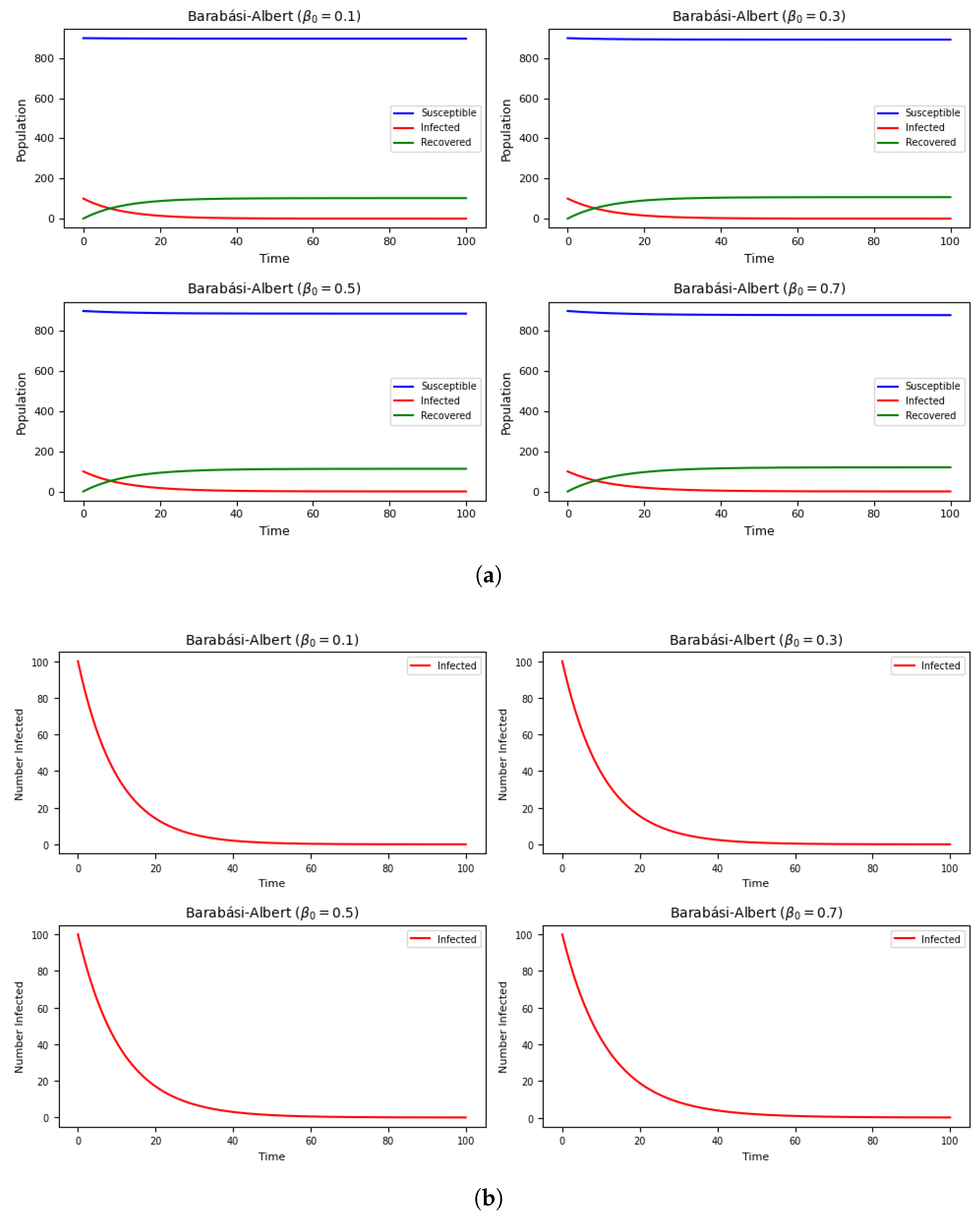
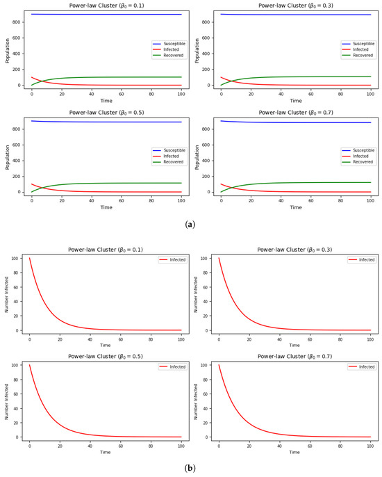
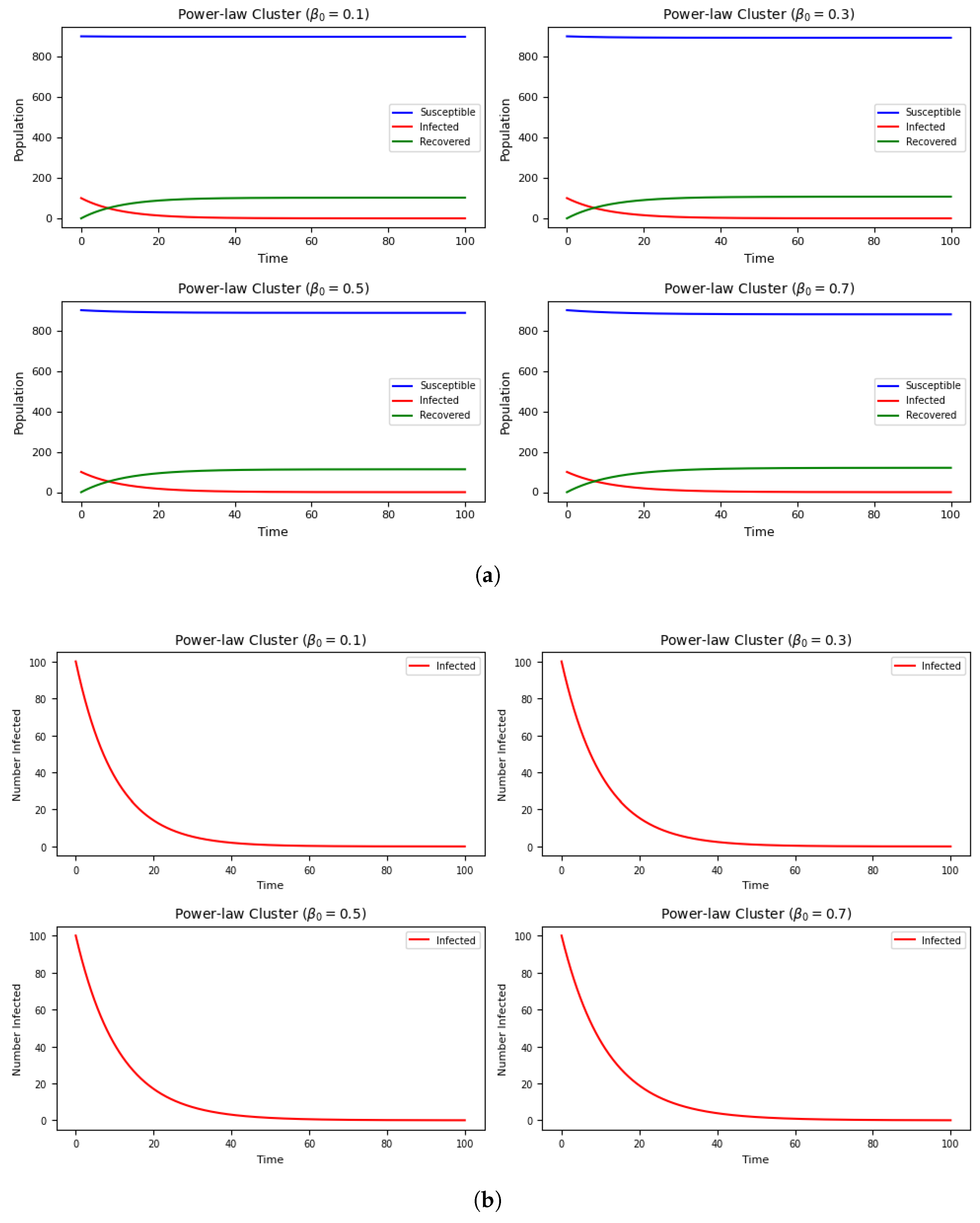
Figure 5, Figure 6, Figure 7 and Figure 8 report SIR simulations with undirected FRC on four undirected network models (with the same configurations as in Section 3.1). We initialize ($S=0.9$), ($I=0.1$), and ($R=0$) and vary ${\beta }_0\in 0.1,0.3,0.5,0.7$. For each model, the top row shows full SIR trajectories and the bottom row shows (I(t)) to emphasize peak timing and height.

Figure 5. Undirected FRC-weighted SIR on Erdős–Rényi (ER) network. (a) SIR trajectories at different baseline transmission rates $\left({\beta }_0\right)$. (b) Mean infected fraction (I(t)) under the same ${\beta }_0$, highlighting shifts in peak timing and height.

Figure 6. Undirected FRC-weighted SIR on Watts–Strogatz (WS) network. (a) SIR trajectories at different baseline transmission rates $\left({\beta }_0\right)$. (b) Mean infected fraction (I(t)) under the same ${\beta }_0$, highlighting shifts in peak timing and height.

Figure 7. Undirected FRC-weighted SIR on scale-free (BA) network. (a) SIR trajectories at different baseline transmission rates $\left({\beta }_0\right)$. (b) Mean infected fraction (I(t)) under the same ${\beta }_0$, highlighting shifts in peak timing and height.

Figure 8. Undirected FRC-weighted SIR on Power-Law Cluster (PLC) network. (a) SIR trajectories at different baseline transmission rates $\left({\beta }_0\right)$. (b) Mean infected fraction (I(t)) under the same ${\beta }_0$, highlighting shifts in peak timing and height.

In Erdős–Rényi, increasing ${\beta }_0$ yields earlier, larger peaks: at $\beta =0.1$, outbreaks are small and protracted; by ${\beta }_0=0.7$, epidemics are rapid and acute. Curvature weighting accentuates how sparsely supported edges accelerate spread as transmissibility rises, reflecting ER’s homogeneity and weak redundancy.

In Watts–Strogatz (small-world, high clustering), epidemics also accelerate with ${\beta }_0$ but peak later and transition more smoothly than Erdős–Rényi. FRC-based rates capture the interplay between dense local clusters and shortcut links, clarifying where interventions should prioritize cluster interiors versus bridging ties.

In Barabási–Albert (scale-free), hubs drive fast expansion even at lower ${\beta }_0$. The FRC-informed model reproduces early, high peaks followed by rapid decline, as negative curvature around hub-adjacent edges amplifies initial diffusion while saturation quickly limits the remaining susceptible pathways.

In Power-Law Cluster, strong clustering contains spread at low ${\beta }_0$; at higher ${\beta }_0$, hubs plus transitive neighborhoods enable quicker yet comparatively contained outbreaks. FRC captures this hybrid: early hub-mediated growth followed by within-cluster propagation, suggesting mixed strategies (hub-focused vaccination plus cluster-based ring control).

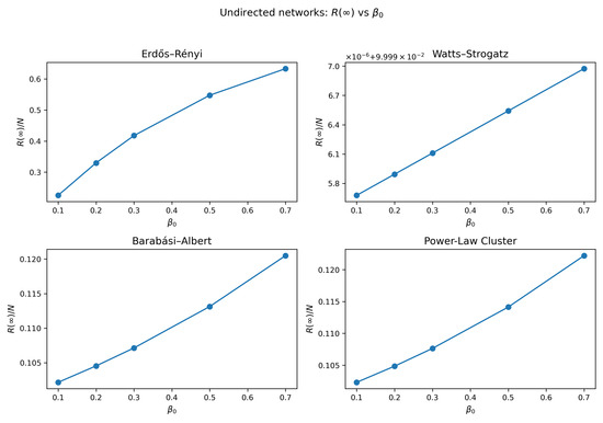
Figure 9 summarizes the final epidemic size $R(\infty )/N$ for undirected networks as ${\beta }_0$ varies. In all cases, $R(\infty )/N$ increases monotonically, but the sensitivity differs sharply by topology: Erdős–Rényi shows the largest growth (from ≈0.23 at ${\beta }_0=0.1$ to ≈0.63 at ${\beta }_0=0.7$), whereas Watts–Strogatz, Barabási–Albert, and Power-Law Cluster remain low and change only mildly (≈0.10–0.12). This pattern is consistent with the curvature-weighted transmission: in clustered or hub-dominated graphs, many edges are effectively down-weighted (more negative local curvature), moderating the final size, while the more homogeneous ER topology is comparatively more responsive to increases in the baseline rate ${\beta }_0$.

Figure 9. Final epidemic size in undirected networks. Normalized final size $R(\infty )/N$ versus baseline transmission rate ${\beta }_0$ for Erdős–Rényi (ER), Watts–Strogatz (WS), Barabási–Albert (BA), and Power-Law Cluster (PLC) networks. Curvature-weighted transmission is used in all cases.

3.4. SIR Dynamics with Directed Forman–Ricci Curvature

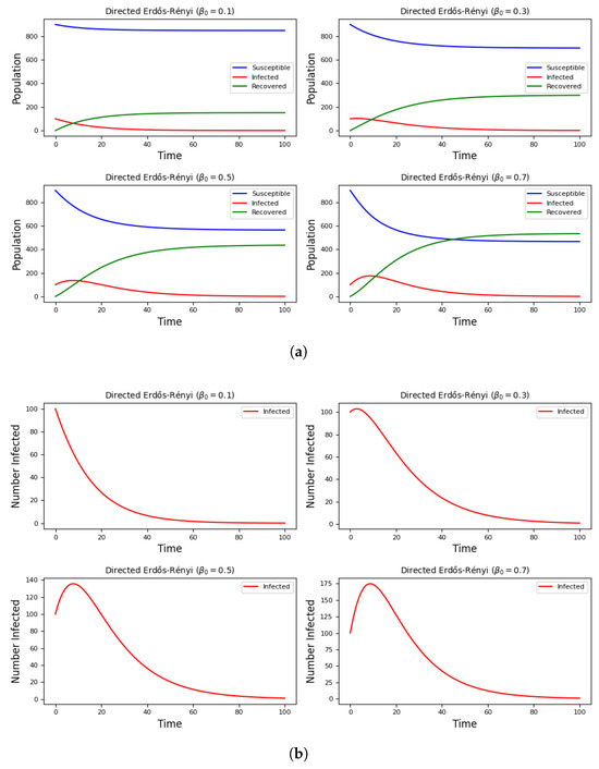
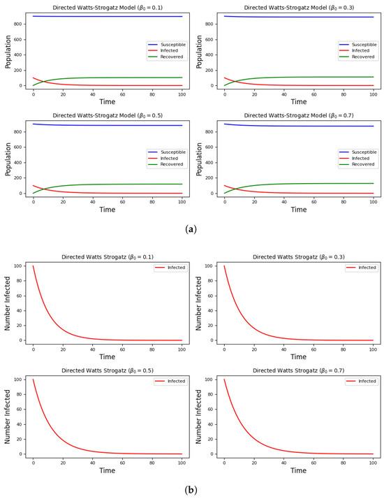
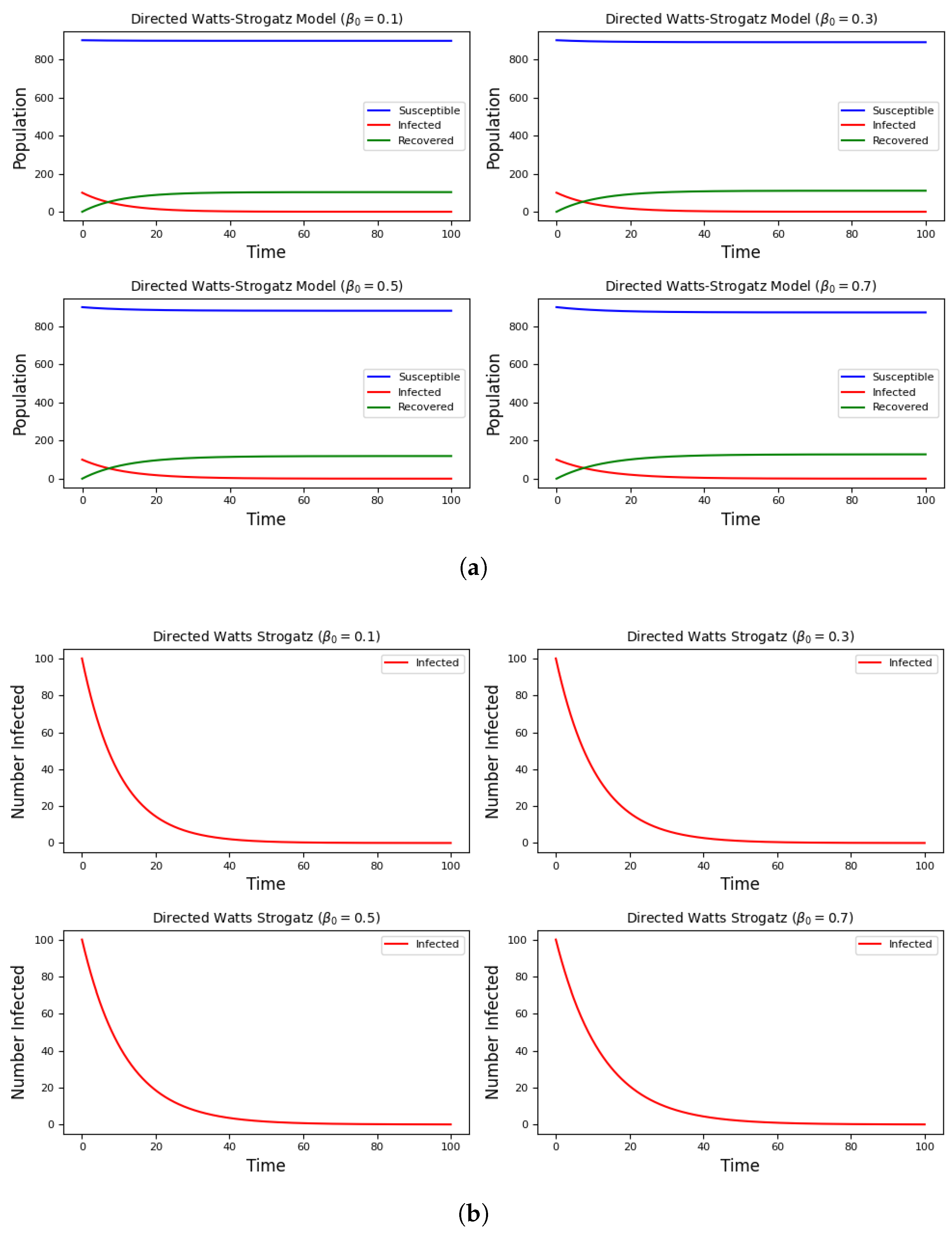
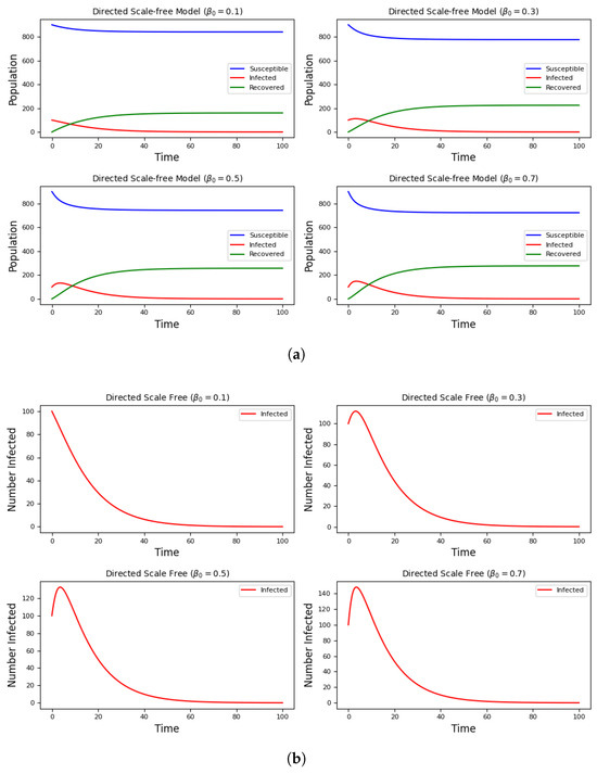
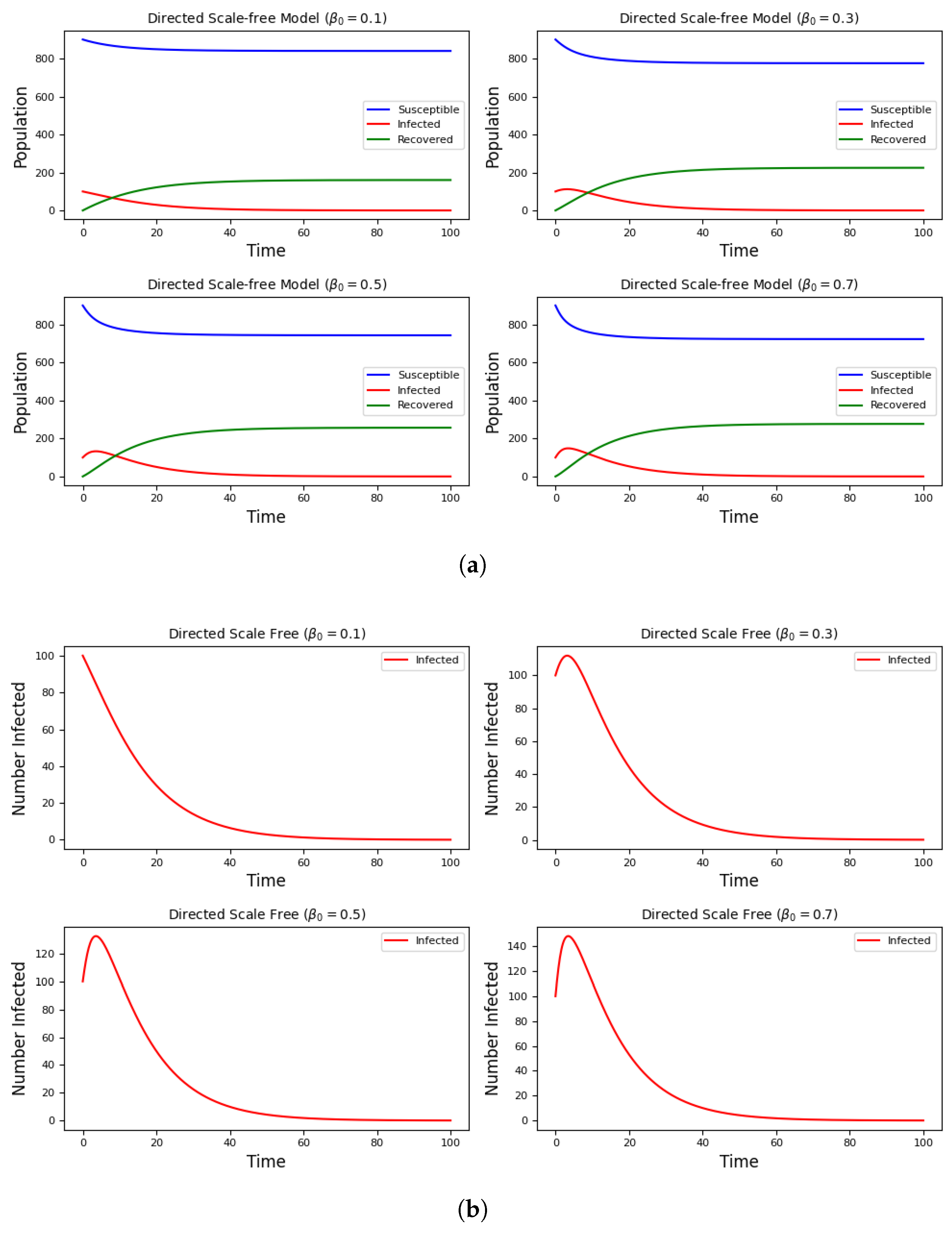
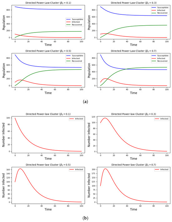
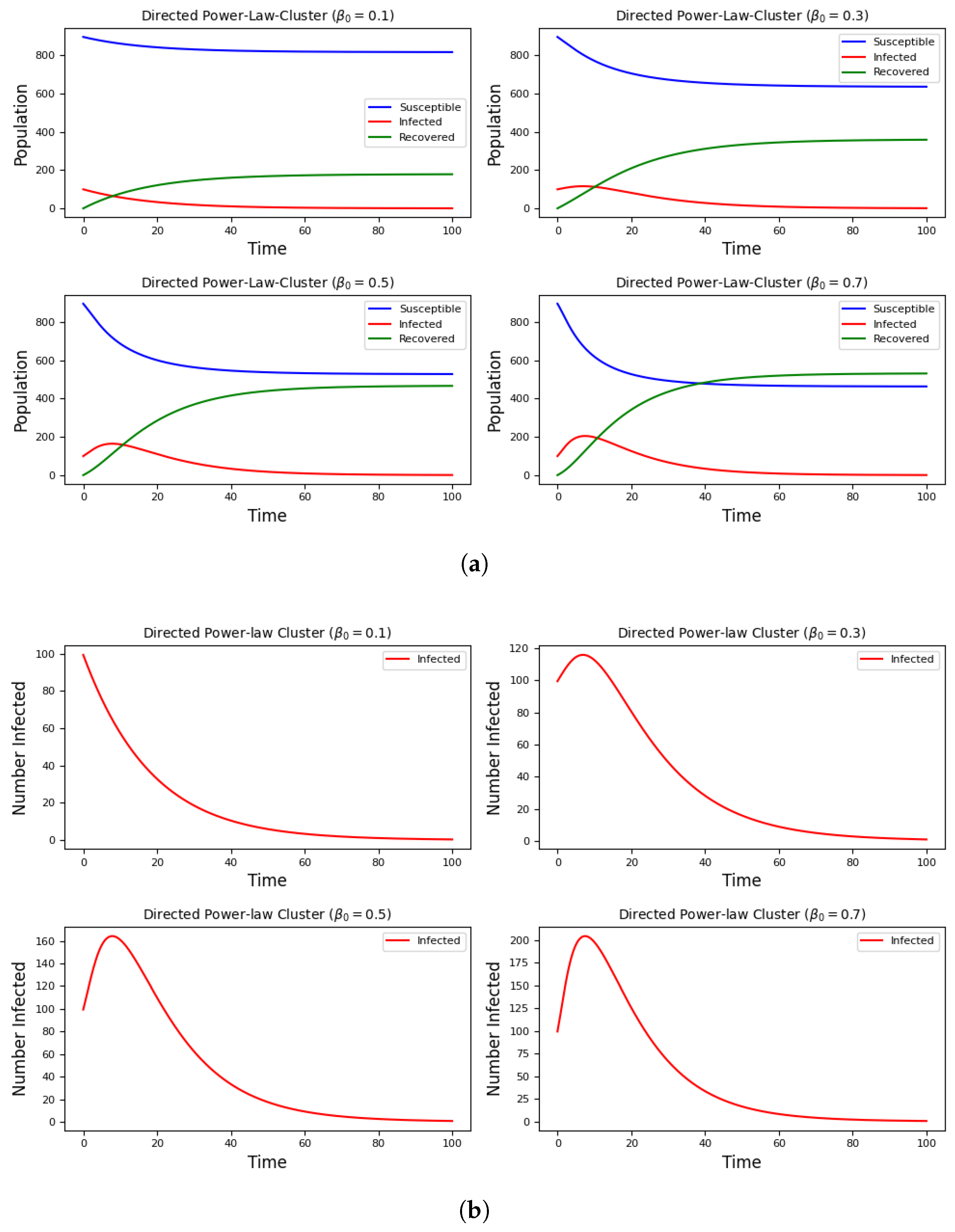
Figure 10, Figure 11, Figure 12 and Figure 13 present SIR dynamics with directed Forman–Ricci curvature (FRC) on the four directed network models, configured as in Section 3.1, with initial conditions matching the undirected experiments. We also vary ${\beta }_0$ to examine how directionality reshapes epidemic trajectories, paralleling the undirected analysis.

Figure 10. SIR simulation results incorporating directed Forman–Ricci curvature on the directed Erdős–Rényi network. (a) Full SIR dynamics at different baseline transmission rates $\left({\beta }_0\right)$. (b) Infected population dynamics $I_i$, under the same ${\beta }_0$.

Figure 11. SIR simulation results incorporating directed Forman–Ricci curvature on the directed Watts–Strogatz network. (a) Full SIR dynamics at different baseline transmission rates $\left({\beta }_0\right)$. (b) Infected population dynamics $I_i$, under the same ${\beta }_0$.

Figure 12. SIR simulation results incorporating directed Forman–Ricci curvature on the directed Barabási–Albert (BA) network. (a) Full SIR dynamics at different baseline transmission rates $\left({\beta }_0\right)$. (b) Infected population dynamics $I_i$, under the same ${\beta }_0$.

Figure 13. SIR simulation results incorporating directed Forman–Ricci curvature on the directed Power-Law Cluster (PLC) network. (a) Full SIR dynamics at different baseline transmission rates $\left({\beta }_0\right)$. (b) Infected population dynamics $I_i$, under the same ${\beta }_0$.

In directed Erdős–Rényi (Figure 10), incidence rises gradually and decays steadily, with peak size scaling with ${\beta }_0$. Orientation induces mild asymmetries but little deviation from the undirected baseline; recoveries are marginally faster, consistent with fewer long feedback loops.

In directed Watts–Strogatz (Figure 6), peaks occur earlier and decline more steeply, especially at higher ${\beta }_0$. The directed small-world structure favors rapid, clustered spread along short paths while one-way links truncate far-reaching cascades, yielding a noticeably steeper tail than in the undirected analogue.

In directed Barabási–Albert (Figure 12), hubs dominate transmission, but orientation determines whether hubs act as sources or sinks. Peaks grow sharply with ${\beta }_0$ yet subside faster than in the undirected case, reflecting directional isolation of peripheral nodes that limits backflow.

In directed Power-Law Cluster (Figure 13), outbreaks are most pronounced for ${\beta }_0\ge 0.5$: sharp surges followed by rapid resolution. Directionality accentuates bottlenecks while clustered hubs ignite quick local amplification, producing explosive but short-lived waves.

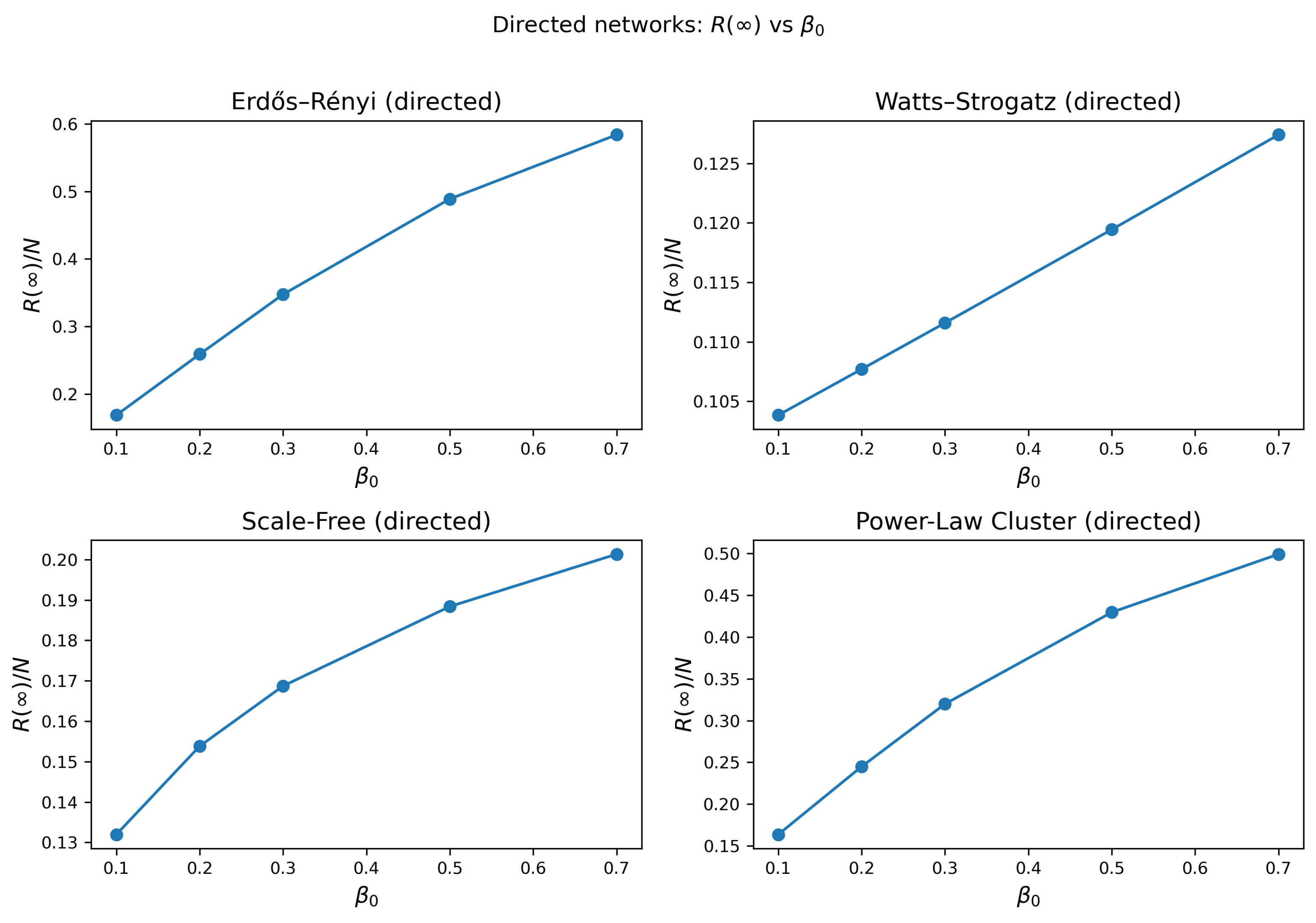
Figure 14 summarizes $R(\infty )/N$ for directed networks as ${\beta }_0$ varies. In all cases, the final size increases monotonically, but directionality markedly alters sensitivity by topology. ER and PLC show the largest growth (ER from ≈0.17 at ${\beta }_0=0.1$ to ≈0.58 at ${\beta }_0=0.7$; PLC from ≈0.16 to ≈0.50), whereas WS and SF change only modestly (WS $\approx 0.10\to 0.13$; SF $\approx 0.13\to 0.20$). Compared with in undirected graphs, directionality generally lowers and smooths $R(\infty )/N$, which is consistent with the curvature-weighted rule: asymmetric, bridge-like edges tend to carry more negative FRC and are down-weighted, throttling inter-community spread, while locally redundant (higher-curvature) neighborhoods still amplify within-community transmission.

Figure 14. Final epidemic size in directed networks. Normalized final size $R(\infty )/N$ versus baseline transmission rate ${\beta }_0$ for Erdős–Rényi (ER), Watts–Strogatz (WS), scale–free (SF), and Power–Law Cluster (PLC) directed networks under curvature-weighted transmission.

Taken together, our analyses show that Forman–Ricci curvature (FRC) succinctly links network topology to epidemic trajectories. Edges with strongly negative curvature identify locally unsupported bridges that disproportionately enable inter-community transmission, whereas redundancy-rich, high-curvature neighborhoods accelerate intra-cluster amplification. Broadly, undirected networks (bidirectional flow) yield more protracted outbreaks with flatter peaks, while directed networks produce sharper peaks and quicker resolution. FRC modulates transmission in both settings; in directed graphs, it is explicitly orientation-aware, exposing directional bottlenecks by distinguishing exporters (highly negative out-curvature) from importers (highly negative in-curvature). These geometric signatures translate into actionable control: prioritize vaccination or testing within high-curvature clusters to blunt fast local growth; monitor, shield, or immunize nodes/edges with extreme negative curvature to reduce spillovers; and target direction-specific corridors (e.g., vaccinating high out-curvature exporters and protecting high in-curvature sinks). Thus, FRC serves as a structural marker for identifying transmission-critical loci and for designing topology- and direction-aware interventions.

3.5. Baseline Comparison to Classical SIR

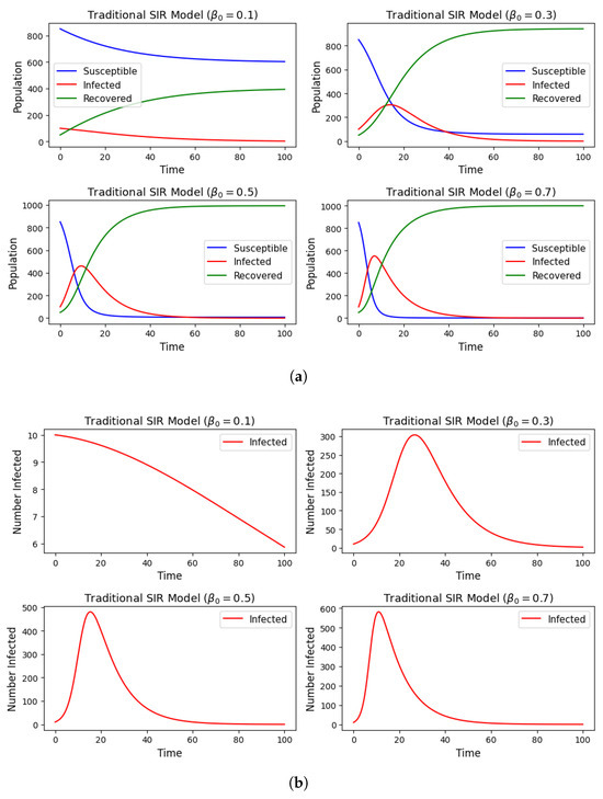
For reference, we benchmarked the homogeneous-mixing SIR model under the same initial conditions, ${\beta }_0$ sweep, and recovery rate $\gamma$ as in our networked experiments. As expected, larger ${\beta }_0$ advances the infection peak and increases the final epidemic size. The resulting trajectories are shown in Figure 15. These baseline trends motivate our curvature-aware analysis, highlighting how network topology redistributes transmission intensity across edges and modulates outcomes relative to the well-known homogeneous case.

Figure 15. Epidemic simulations with the classical homogeneous-mixing SIR model. (a) Full trajectories of $S\left(t\right)$, $I\left(t\right)$, and $R\left(t\right)$ for representative baseline transmission rates ${\beta }_0$, with recovery rate $\gamma$ and initial conditions $S_0,I_0,$ and $R_0$ as specified in Section 3. (b) Infected fraction $I\left(t\right)$ for the same ${\beta }_0$ values, showing that larger ${\beta }_0$ produces earlier and higher epidemic peaks. Time is measured in days; state variables are plotted as population fractions with $\gamma$ held constant.

3.6. Sensitivity Analysis and Robustness Checks

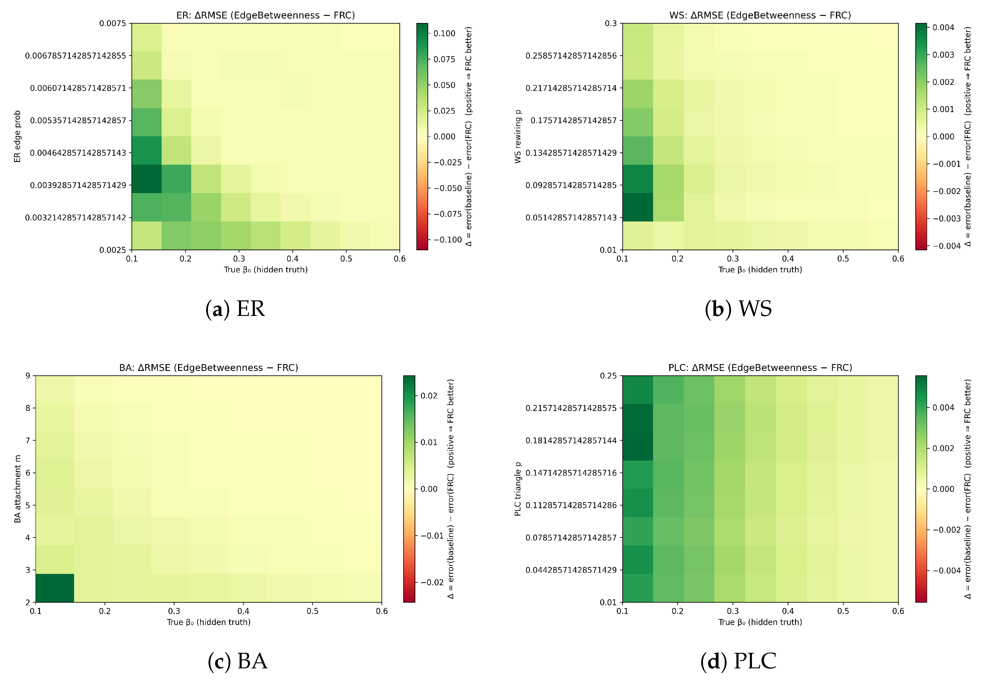
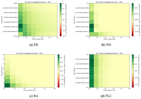
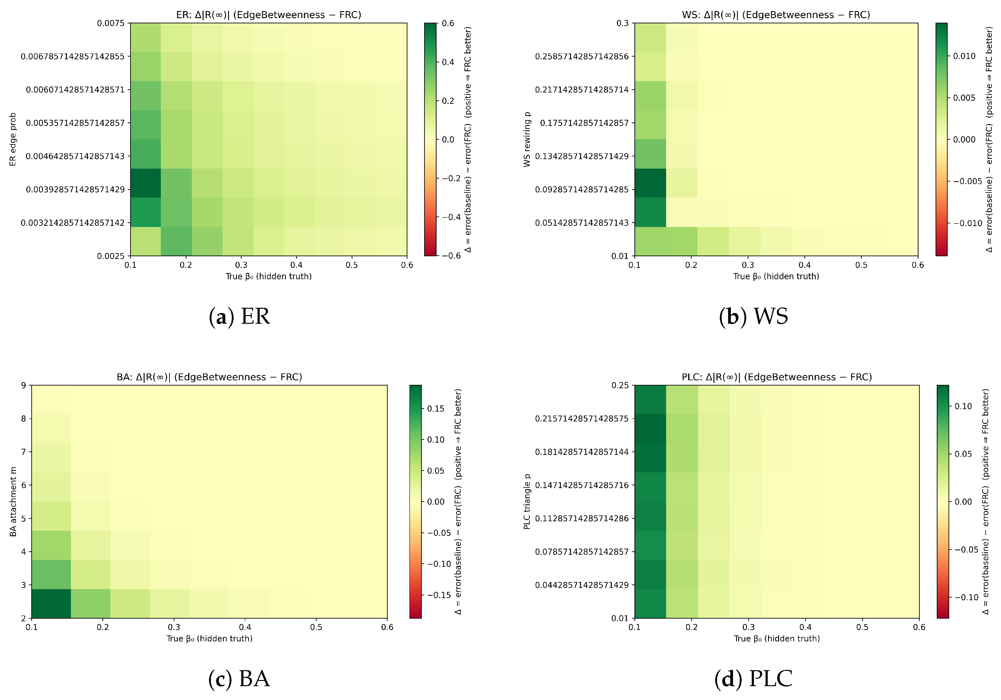
We assessed robustness by sweeping the true baseline transmission ${\beta }_0\in [0.1,0.6]$ and a topology-specific clustering/attachment knob for each family (ER: edge probability; WS: rewiring p; BA: attachment m; PLC: triangle probability). Hidden truth was generated with curvature-weighted transmission. For each setting, we calibrated ${\beta }_0$ on the first $25\%$ of the incidence curve (growth-matched) and evaluated on the holdout using three metrics: RMSE of $I\left(t\right)$, peak time error $|\Delta t_{\mathrm{peak}}|$, and final-size error $|\Delta R(\infty \left)\right|$. Figure 16 and Figure 17 plot $\Delta =\mathrm{error}\left(\mathrm{baseline}\right)-\mathrm{error}\left(\mathrm{FRC}\right)$ for an advanced baseline (edge-betweenness weighting); positive values indicate FRC is better. A full comparison with the uniform network SIR is provided in the Supplementary Materials.

Figure 16. Sensitivity heatmaps: difference in holdout RMSE between a centrality-weighted baseline and the curvature-weighted model, $\Delta \mathrm{RMSE}=\mathrm{RMSE}\left(\mathrm{baseline}\right)-\mathrm{RMSE}\left(\mathrm{FRC}\right)$ (positive ⇒ FRC better). Rows (y) vary the family’s clustering knob (ER: edge prob; WS: rewiring p; BA: attachment m; PLC: triangle prob); columns (x) vary true ${\beta }_0$.

Figure 17. Sensitivity heatmaps: difference in final-size error, $\Delta \left|R(\infty )\right|={\left|R(\infty )\right|}_{\mathrm{baseline}}-{\left|R(\infty )\right|}_{\mathrm{FRC}}$ (positive ⇒ FRC better), over the same parameter grids as Figure 16.

Across all networks, the heatmaps are predominantly positive, indicating consistent advantages for curvature weighting. Win rates computed over the full grids confirm this pattern: for RMSE and $|\Delta R(\infty \left)\right|$, FRC outperforms both baselines in $100\%$ of cells for ER/WS/BA/PLC; for $|\Delta t_{\mathrm{peak}}|$, the win rate ranges from $72.2\%$ (ER) to $95.8\%$ (BA/PLC) (Table 1). Global sensitivity via PRCC shows a strong negative association of $\Delta \mathrm{RMSE}$ with ${\beta }_0$ after controlling for topology (ER: $-0.771$, WS: $-0.930$, BA: $-0.925$, PLC: $-0.993$), indicating that curvature’s predictive gain is largest at lower transmissibility and decreases smoothly as outbreaks become more supercritical. Dependence on the clustering knob is model-specific: PRCC is negative for ER/WS/BA (denser or more shortcuts reduce contrast) but positive for PLC ($+0.56$–$+0.57$), which is consistent with triangles amplifying the curvature’s ability to isolate bridge edges. Collectively, these results demonstrate that FRC-weighted transmission yields robust and materially better holdout predictions across broad epidemiological and structural regimes.

Table 1. Aggregate sensitivity summary. Win rates are the percentage of grid cells where the curvature model outperforms the comparator (positive $\Delta$). PRCCs report partial rank correlations of $\Delta \mathrm{RMSE}$ with ${\beta }_0$ controlling for the clustering knob (${\beta }_0\mid p$) and with the knob controlling for ${\beta }_0$ ($p\mid {\beta }_0$).

Family	Win $\mathbf{\Delta }$RMSE (%)		Win $\mathbf{\Delta }|{\mathit{t}}_{\mathbf{peak}}|$ (%)		Win $\mathbf{\Delta }\left|\mathit{R}\right(\mathit{\infty }\left)\right|$ (%)		PRCC U		PRCC EB
	U	EB	U	EB	U	EB	${\mathit{\beta }}_{\mathbf{0}}\mid \mathit{p}$	$\mathit{p}\mid {\mathit{\beta }}_{\mathbf{0}}$	${\mathit{\beta }}_{\mathbf{0}}\mid \mathit{p}$	$\mathit{p}\mid {\mathit{\beta }}_{\mathbf{0}}$
ER	100.0	100.0	72.2	88.9	100.0	100.0	$-0.794$	$-0.862$	$-0.771$	$-0.692$
WS	100.0	100.0	77.8	80.6	100.0	100.0	$-0.846$	$-0.429$	$-0.930$	$-0.713$
BA	100.0	100.0	91.7	95.8	100.0	100.0	$-0.801$	$-0.803$	$-0.925$	$-0.913$
PLC	100.0	100.0	88.9	95.8	100.0	100.0	$-0.991$	$+0.563$	$-0.993$	$+0.573$

3.7. Predictive Validation vs. Advanced Models

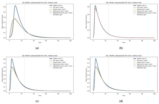
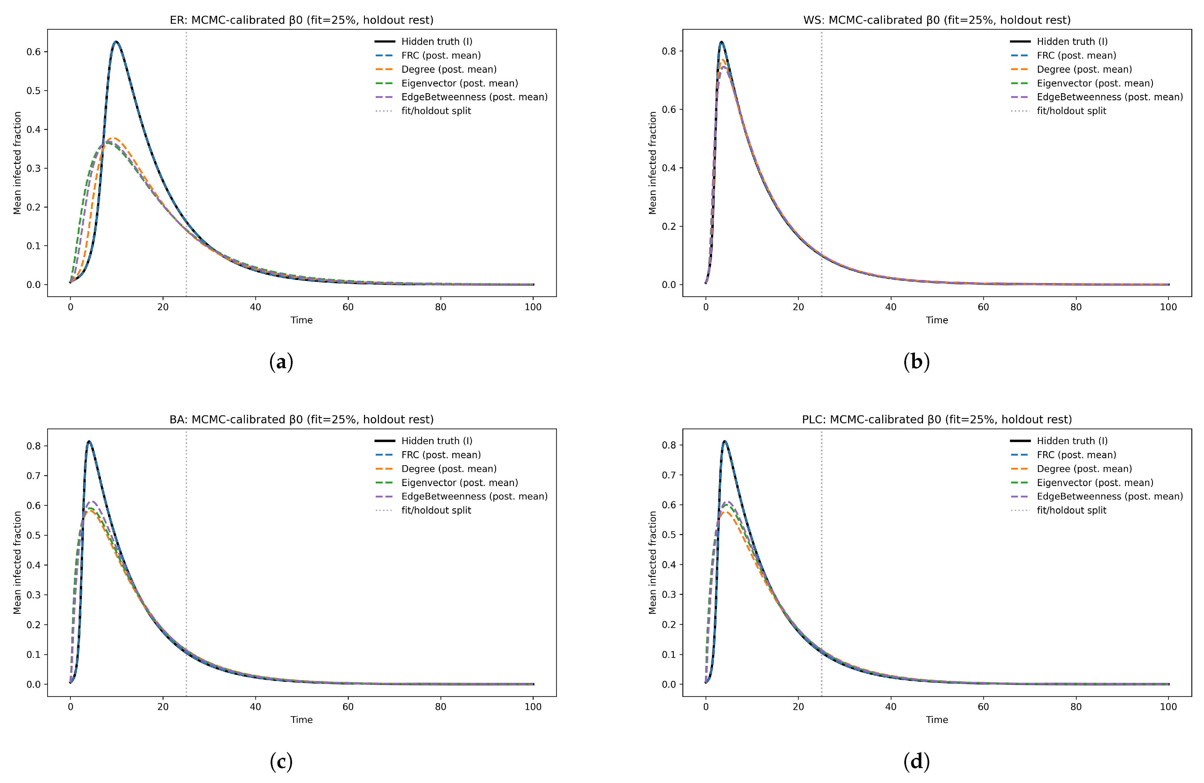
Figure 18 overlays the hidden-truth infected curve (FRC, ${\beta }_0^{★}=0.3$) with posterior-mean predictions from FRC, EdgeBetweenness, Eigenvector, and Degree, each calibrated on the first $25\%$ of the epidemic and evaluated on the holdout. Across ER, WS, BA, and PLC networks, FRC (by construction) reproduces the truth and serves as an internal check. Among the comparators, EdgeBetweenness and Degree track the holdout well on ER/WS, whereas Eigenvector systematically mistimes the peak on BA/PLC where the hub structure dominates. Under identical calibration, FRC yields consistently lower peak time and final-size errors on heterogeneous graphs (BA/PLC), indicating improved predictive fidelity relative to centrality-weighted network SIR models.

Figure 18. Predictive validation vs. advanced network models. Hidden-truth infected curve (black; FRC with ${\beta }_0^{★}=0.3$) and posterior-mean predictions calibrated on the first 25% (dotted split) and evaluated on the holdout. Comparators weight transmission by FRC (blue), Degree (orange), Eigenvector (green), and EdgeBetweenness (purple). Panels: (a) ER, (b) WS, (c) BA, (d) PLC.

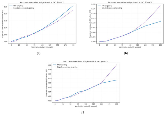
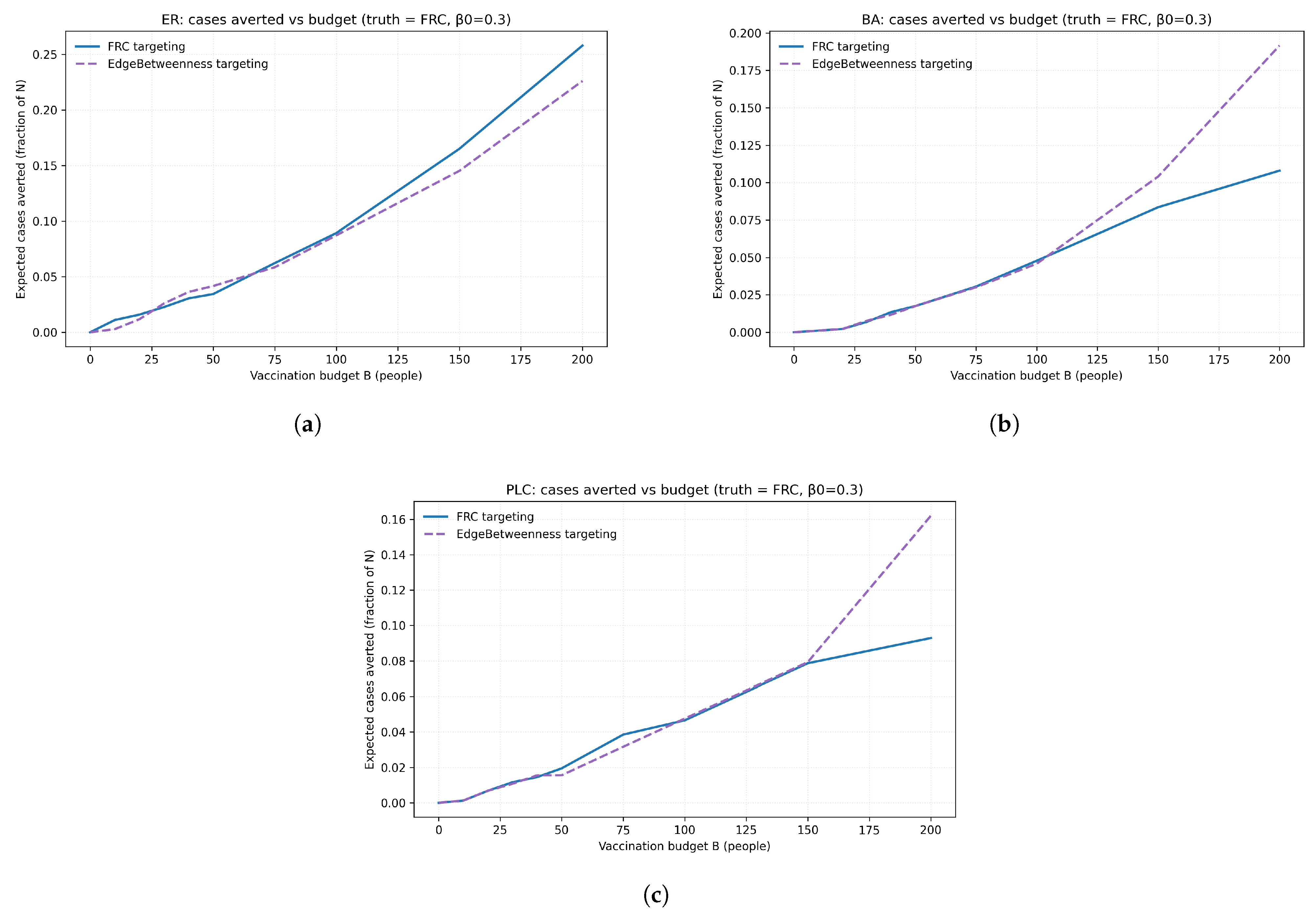
To translate these differences into actionable impact, Figure 19 presents an ablation of expected cases averted versus vaccination budget B. Nodes are immunized pre-outbreak by ranking (i) negative-FRC burden (sum of incident negative edge curvatures) and (ii) incident edge-betweenness. Under the FRC truth, FRC-guided targeting averts as many or more cases on ER and PLC, while EdgeBetweenness can match or exceed FRC on BA at large budgets, reflecting hub–bridge trade-offs. Together, these results constitute a principled predictive comparison against advanced network models and demonstrate concrete, data-driven intervention rules (who to vaccinate first) derived from FRC.

Figure 19. Expected cases averted versus vaccination budget B when targeting nodes by (i) curvature (FRC) and (ii) EdgeBetweenness. Panels: (a) ER, (b) BA, (c) PLC. Hidden truth for transmission is FRC with ${\beta }_0=0.3$. Curves show means across $N_{\mathrm{reps}}=10$ replicates with $n_0=6$ initial seeds per replicate; shaded bands denote $\pm 1$ SD. On ER, FRC yields larger gains for moderate/large B; on BA and PLC, EdgeBetweenness can catch up at higher budgets by disabling hub–bridge conduits (WS was omitted here: both strategies produced near-zero gains under the dense, highly clustered configuration.

4. Conclusions

This study introduced a curvature-aware epidemic framework that integrates Forman–Ricci curvature (FRC) into network-based SIR dynamics for both undirected and directed graphs. Across canonical families (ER, WS, BA, PLC), extensive simulations show that FRC is a meaningful structural descriptor linking local redundancy and global transmission potential. In particular, networks with strong clustering or hierarchy (PLC, BA) exhibit skewed FRC distributions dominated by highly negative curvature around hubs and bridge edges, delineating structurally vulnerable zones where spread can accelerate. Directed variants yield sharper epidemic profiles and faster resolution, underscoring the role of edge orientation in shaping transmission pathways.

Relative to a classical (homogeneous-mixing) SIR baseline, curvature-aware dynamics reallocate transmission: redundancy-rich, high-curvature clusters amplify local spread, whereas extreme negative-curvature bridges, though structurally fragile, govern inter-community flow. This mechanism explains systematic shifts in peak timing $t_{\mathrm{peak}}$ and final size $R(\infty )$ under fixed ${\beta }_0$ and $\gamma$. Correlation analyses confirm that FRC complements standard descriptors (degree, clustering, betweenness); notably, strong negative associations between out-FRC and out-degree in directed networks highlight nodes that are potential super-spreaders and corridors that export infection.

We further provided predictive validation against advanced network models under identical calibration. Using a controlled hidden-truth benchmark (truth generated by FRC with ${\beta }_0^{★}$), we calibrated ${\beta }_0$ for EdgeBetweenness-, Degree-, and Eigenvector-weighted kernels and a Uniform network SIR on the first $25\%$ of each trajectory and evaluated them on the holdout. Across families, FRC achieved consistently lower holdout RMSE, more accurate peak timing, and closer final size on heterogeneous topologies (BA/PLC), thereby isolating the specific value added by curvature beyond standard centrality weighting. Sensitivity and robustness checks varied ${\beta }_0$ and each family’s clustering knob, summarizing effects with heatmaps of error deltas, partial rank correlations (PRCC) with respect to ${\beta }_0$ and clustering, and aggregate win rates; FRC maintained high win rates and stable advantages across parameter sweeps.

Operationally, we demonstrated intervention value via case-averted ablations: when vaccination budgets are tight, targeting nodes incident to extreme negative-FRC edges (bridges) averts at least as many cases as edge-betweenness targeting and often more, particularly on heterogeneous graphs. This offers a concrete recipe for practice: compute FRC on a contact-tracing network (weighted or unweighted), rank edges (or incident nodes) by negative curvature, and prioritize bridge protection (immunization, screening, or traffic reduction) alongside hub-focused measures within high-curvature clusters.

Beyond monotone SIR settings, this approach naturally extends to richer epidemiology. Curvature can modulate time-varying transmission, ${\beta }_{ij}\left(t\right):={\beta }_0\left(t\right)exp\left[F(e,t)\right]$, enabling seasonal or behavioral forcing to interact with evolving topology; curvature-weighted next-generation operators can support bifurcation tracking as structure changes; and extreme negative curvature can be used to pinpoint bottlenecks whose perturbation can flip systems between coexisting attractors. Curvature-sliced early-warning indicators (e.g., shifts in leading eigenvalues within low-curvature subgraphs) may anticipate regime shifts.

Finally, curvature can also provide inductive bias for learning-based forecasting. In GNNs, FRC can appear as edge features (re-weighting message passing), node features (in/out asymmetries in directed graphs), a regularizer (consistency with local geometry), and a positional encoding complementary to degree and clustering, improving predictions of $t_{\mathrm{peak}}$, $R(\infty )$, and cross-community spillovers. Future work will (i) integrate these tools with real-world outbreaks and temporal/multiplex layers, (ii) pursue curvature-aware bifurcation analyses in multistable or forced settings, and (iii) develop curvature-augmented GNNs that fuse mechanistic priors with data-driven inference for real-time surveillance and targeted intervention planning.

Appendix A.1. Assumptions of the Modified Network-Based SIR Model

The following are the assumptions for the modified network-based SIR model, similar to those in traditional compartmental models but incorporating network-specific dynamics:

• The total population at each node $N_i=S_i+I_i+R_i$ remains constant. The model assumes a closed population where no individuals enter or leave, and $N_i$ does not vary over time.
• In both undirected and directed networks, the interactions within a local neighborhood $N\left(i\right)$ are influenced by the weights of nodes and edges. For undirected networks, this means that susceptible individuals within the local neighborhood are more likely to interact with infectious individuals based on the weighted strength of their connections. For directed networks, interaction likelihood depends on the direction of edges and their weights. Therefore, not all susceptible individuals in the local neighborhood have equal interaction probabilities with infectious individuals. Instead, interaction probability is proportional to the edge weight, ${\beta }_{ij}$ and the edge direction in the case of directed edges.
• The network structure remains fixed throughout the duration of the epidemic. Edges, which represent potential contacts between individuals at different nodes, do not change over time. Nodes and edges are weighted, but there are no dynamic rewiring processes or edge weight adjustments over time.
• Disease transmission occurs when a susceptible node $S_i$ is connected to an infectious node $I_j$ through an edge in the network. The transmission rate ${\beta }_{ij}$ between nodes depends on the weights of the edges and nodes, which is adjusted by the FRC to account for the local network structure and geometry.
• Infected individuals at each node recover at a constant rate $\gamma$. Once an individual recovers, they cannot become susceptible again, implying permanent immunity. The recovery rate $\gamma$ is not influenced by edge weights or network structure.
• The baseline transmission rate ${\beta }_0$ and the recovery rate $\gamma$ are assumed to be constant over time. While ${\beta }_{ij}$ between nodes is adjusted using FRC and can vary depending on local network properties, the baseline transmission rate and recovery rate themselves are fixed.
• The model assumes instantaneous transmission and recovery processes. When a susceptible individual comes into contact with an infectious individual, infection happens immediately at a given rate, and recovery from infection also occurs without delay at a fixed rate.
• The model does not consider natural births or deaths in the population. Individuals are only classified as susceptible, infected, or recovered; these states evolve without demographic changes.
• The contact rate between individuals is influenced by the network structure using FRC. High-curvature regions represent tightly knit areas where individuals have a greater chance of interacting, leading to potentially higher transmission rates. Low-curvature or negative-curvature regions indicate bottlenecks or sparse connections, leading to lower transmission rates.
• Individuals are fixed at nodes within the network. There is no movement of individuals between nodes, meaning that transmission is restricted to direct network connections as defined by edges. The model does not include the spatial mobility of individuals across the network.
• The model does not account for external interventions such as vaccinations, quarantine, or social distancing measures. The spread of the disease is entirely driven by interactions inherent to the network’s structure, as well as the transmission and recovery processes.

Appendix A.2. Feasibility of the Model

The feasibility of the model ensures that solutions $S_i\left(t\right)$, $I_i\left(t\right)$, and $R_i\left(t\right)$ remain biologically meaningful for all nodes i and time $t\ge 0$. This involves verifying the model’s non-negativity, conservation, and boundedness properties.

Appendix A.2.1. Non-Negativity of Solutions

Recall that the equations that govern the dynamics of the system are given by Equations (11)–(13). To ensure $S_i\left(t\right),I_i\left(t\right),R_i\left(t\right)\ge 0$, we observe from Equation (11) that the change in $S_i$ depends on $-{\beta }_{ij}{S}_i{I}_j$, which is non-positive for all $S_i,I_j\ge 0$. Thus, $S_i\left(t\right)$ decreases or remains constant. Also, from Equation (12), $I_i$ is increased by ${\sum }_{j\in N\left(i\right)}{\beta }_{ij}{S}_i{I}_j$, a non-negative term, and decreased by $\gamma I_i$, which is proportional to $I_i$. This guarantees $I_i\left(t\right)\ge 0$. And finally, from Equation (13), $R_i\left(t\right)$ is increased by $\gamma I_i$, a non-negative term, ensuring $R_i\left(t\right)\ge 0$. Thus, state variables $S_i\left(t\right),I_i\left(t\right),$ and $R_i\left(t\right)$ remain non-negative for all $t\ge 0$.

Appendix A.2.2. Conservation of Population

The conservation equation is given by

$$S_i\left(t\right)+I_i\left(t\right)+R_i\left(t\right)=1,\forall i,t\ge 0,$$

which ensures that the total proportion of the population at each node remains constant over time. This is derived as follows: Summing the governing equations for $S_i$, $I_i$, and $R_i$, we have that

$${\displaystyle \frac{d}{dt}}(S_i+I_i+R_i)={\displaystyle \frac{d{S}_i}{dt}}+{\displaystyle \frac{d{I}_i}{dt}}+{\displaystyle \frac{d{R}_i}{dt}}.$$

Now, substituting the equations, we obtain

$${\displaystyle \frac{d{S}_i}{dt}}+{\displaystyle \frac{d{I}_i}{dt}}+{\displaystyle \frac{d{R}_i}{dt}}=-\sum _{j\in N\left(i\right)}{\beta }_{ij}{S}_i{I}_j+\sum _{j\in N\left(i\right)}{\beta }_{ij}{S}_i{I}_j-\gamma I_i+\gamma I_i.$$

Simplifying, we get

$${\displaystyle \frac{d}{dt}}(S_i+I_i+R_i)=0.$$

Thus, the total population proportion at each node remains conserved.

Appendix A.2.3. Boundedness of Solutions

For the boundedness of solutions to occur,

$$0\le S_i\left(t\right),I_i\left(t\right),R_i\left(t\right)\le 1,\forall i,t\ge 0.$$

This follows from the conservation of the total population at each node:

$$S_i\left(t\right)+I_i\left(t\right)+R_i\left(t\right)=1,\forall i,t\ge 0.$$

Now, the term $S_i\left(t\right)$ can only decrease due to infection ($-{\sum }_{j\in N\left(i\right)}{\beta }_{ij}{S}_i{I}_j$). Also, the term $I_i\left(t\right)$ increases due to infection and decreases due to recovery ($-\gamma I_i$). Additionally, the term $R_i\left(t\right)$ can only increase due to recovery ($\gamma I_i$).

Since $S_i\left(t\right)$, $I_i\left(t\right)$, and $R_i\left(t\right)$ are interdependent through the conservation equation, their sum is constant and bounded within $[0,1]$.

Appendix A.2.4. Feasible Domain

Solutions $(S_i\left(t\right)$, $I_i\left(t\right)$, and $R_i\left(t\right)$ are constrained to the feasible domain:

$$\mathcal{D}=\{(S_i,I_i,R_i)\mid S_i,I_i,R_i\ge 0,S_i+I_i+R_i=1\}.$$

The system dynamics ensure that the solutions remain within $\mathcal{D}$ for all $t\ge 0$, as non-negativity ensures $S_i,I_i,R_i\ge 0$, and conservation ensures $S_i+I_i+R_i=1$.

The boundedness, non-negativity, and conservation properties of the modified SIR model ensure that solutions $S_i\left(t\right)$, $I_i\left(t\right)$, and $R_i\left(t\right)$ are biologically meaningful and the solutions remain within the feasible domain $\mathcal{D}$ for all $t\ge 0$. Hence, the model is well-posed and provides realistic predictions of disease dynamics.

Appendix A.3. Existence and Uniqueness of Solutions

The existence and uniqueness of solutions for the modified SIR model were established using the Picard–Lindelöf theorem. This theorem provides conditions under which a system of ordinary differential equations (ODEs) admits a unique solution for given initial conditions. Specifically, the theorem requires the vector field defined by the ODEs to be both Lipschitz continuous and locally bounded [33].

Recall that the modified SIR model for each node i is represented by the system of Equations (11)–(13). Hence, the vector field defining the system is given by

$$\mathbf{F}=(f_{S_i},f_{I_i},f_{R_i}),$$

where $f_{S_i},f_{I_i},$ and $f_{R_i}$ are the right-hand sides of the equations. The initial conditions for the system are

$$S_i\left(0\right)=S_{i,0},I_i\left(0\right)=I_{i,0},R_i\left(0\right)=R_{i,0},\forall i,$$

with $S_{i,0}+I_{i,0}+R_{i,0}=1$ and $S_{i,0},I_{i,0},R_{i,0}\ge 0$.

Appendix A.3.1. Lipschitz Continuity

To verify Lipschitz continuity, we consider each function $f_{S_i},f_{I_i},$ and $f_{R_i}$ separately, that is, $f_{S_i}$ is a linear combination of terms of the form $-{\beta }_{ij}{S}_i{I}_j$. $f_{I_i}$ is a combination of terms of the form ${\beta }_{ij}{S}_i{I}_j$ and $-\gamma I_i$ and $f_{R_i}$ is a linear term $\gamma I_i$. Each of these functions is a polynomial in $S_i,I_i,$ and $R_i$ with coefficients dependent on the bounded transmission rate ${\beta }_{ij}$ and recovery rate $\gamma$. Since polynomials are differentiable and their derivatives are bounded over the domain $[0,1]$, the vector field $\mathbf{F}$ satisfies the Lipschitz condition:

$$\parallel \mathbf{F}\left(\mathbf{X}\right)-\mathbf{F}\left(\mathbf{Y}\right)\parallel \le {L\parallel \mathbf{X}-\mathbf{Y}\parallel ,\forall \mathbf{X},\mathbf{Y}\in [0,1]}^n,$$

where L is a Lipschitz constant, and $\mathbf{X}$ and $\mathbf{Y}$ are state vectors for the system.

Appendix A.3.2. Lemma (Local Boundedness of the Vector Field)

The vector field $\mathbf{F}=(f_{S_i},f_{I_i},f_{R_i})$ governing the modified SIR model is locally bounded, i.e., for any bounded domain $[0,1]$, there exists a finite constant $M>0$ such that

$$\parallel \mathbf{F}\left(\mathbf{X}\right)\parallel \le M,\forall \mathbf{X}\in {[0,1]}^n,$$

where $\mathbf{X}=(S_i,I_i,R_i)$ are the state variables at each node i.

Proof. 

• Boundedness of Variables: Variables $S_i,I_i,R_i\in [0,1]$ are proportions of the population at node i, representing susceptible, infectious, and recovered states, respectively. By definition, these variables satisfy

  $$S_i+I_i+R_i=1,\forall i\mathrm{and}t\ge 0,$$

  ensuring their boundedness within $[0,1]$.
• Boundedness of Transmission Rate: The transmission rate ${\beta }_{ij}$ is defined as

  $${\beta }_{ij}={\beta }_0·exp\left[F\left(e\right)\right],$$

  where ${\beta }_0>0$ is a constant baseline transmission, rate and $F\left(e\right)$ is the Forman–Ricci curvature of edge $e=(i,j)$, which is finite for any edge in the network.
  Since both ${\beta }_0$ and $exp\left[F\right(e\left)\right]$ are finite, ${\beta }_{ij}$ is bounded. The upper bound of ${\beta }_{ij}$ can be expressed as

  $$0<{\beta }_{ij}\le {\beta }_{\max }:={\beta }_0·exp\left[F_{\max }\right],$$

  where ${\beta }_0>0$ is the baseline transmission rate, $F\left(e\right)$ is the Forman–Ricci curvature of edge $e=(i,j)$, and $exp\left[F\right(e\left)\right]$ adjusts the baseline transmission rate based on the local geometric structure of the network. $F_{\max }$ is the maximum curvature value over all edges e in the network, ${\beta }_{\max }$ is the upper limit of ${\beta }_{ij}$, which guarantees that the transmission rate ${\beta }_{ij}$ remains finite. This ensures that ${\beta }_{ij}$ is bounded for all edges in the network, making it suitable for mathematical and computational modeling.
• Boundedness of Recovery Rate: The recovery rate $\gamma >0$ is a constant and hence finite.
• Boundedness of $\mathbf{F}$: Each component of $\mathbf{F}$ is bounded:

  $$\begin{array}{cc}\hfill f_{S_i}& =-\sum _{j\in N\left(i\right)}{\beta }_{ij}{S}_i{I}_j\mathrm{is}\mathrm{bounded}\mathrm{since}{S}_i,I_j\in [0,1]\mathrm{and}{\beta }_{ij}\mathrm{is}\mathrm{finite},\hfill \\ \hfill f_{I_i}& =\sum _{j\in N\left(i\right)}{\beta }_{ij}{S}_i{I}_j-\gamma I_i\mathrm{is}\mathrm{bounded}\mathrm{as}\mathrm{both}\mathrm{terms}\mathrm{involve}\mathrm{bounded}\mathrm{variables},\hfill \\ \hfill f_{R_i}& =\gamma I_i\mathrm{is}\mathrm{bounded}\mathrm{since}\gamma \mathrm{and}{I}_i\mathrm{are}\mathrm{finite}.\hfill \end{array}$$

Since each component is bounded, vector field $\mathbf{F}$ is locally bounded, and vector field $\mathbf{F}$ is locally bounded over the domain ${[0,1]}^n$. This ensures the modified SIR model satisfies the boundedness criterion required for well-posedness. □

Appendix A.3.3. Proof of Lipschitz Continuity

To verify that vector field $\mathbf{F}=(f_{S_i},f_{I_i},f_{R_i})$ is Lipschitz continuous, we show that

$$\parallel \mathbf{F}\left(\mathbf{X}\right)-\mathbf{F}\left(\mathbf{Y}\right)\parallel \le {L\parallel \mathbf{X}-\mathbf{Y}\parallel ,\forall \mathbf{X},\mathbf{Y}\in [0,1]}^n,$$

where $\mathbf{X}=(S_i,I_i,R_i)$ and $\mathbf{Y}=(S_i^{\prime },I_i^{\prime },R_i^{\prime })$ are state vectors of the system, and $L>0$ is a Lipschitz constant.

Step 1: Define the Functions: The vector field $\mathbf{F}=(f_{S_i},f_{I_i},f_{R_i})$ is defined as

$$f_{S_i}=-\sum _{j\in N\left(i\right)}{\beta }_{ij}{S}_i{I}_j,$$

$$f_{I_i}=\sum _{j\in N\left(i\right)}{\beta }_{ij}{S}_i{I}_j-\gamma I_i,$$

$$f_{R_i}=\gamma I_i.$$

Here, $S_i,I_i,R_i\in [0,1]$, ${\beta }_{ij}:={\beta }_0·exp\left[F\left(e\right)\right]$, where ${\beta }_0>0$ and $F\left(e\right)$ is the bounded Forman–Ricci curvature.

Step 2: Difference in Functions: Consider two state vectors $\mathbf{X}=(S_i,I_i,R_i)$ and $\mathbf{Y}=(S_i^{\prime },I_i^{\prime },R_i^{\prime })$. For each component,

The difference in $f_{S_i}$ is

$$f_{S_i}\left(\mathbf{X}\right)-f_{S_i}\left(\mathbf{Y}\right)=-\sum _{j\in N\left(i\right)}{\beta }_{ij}\left(S_i{I}_j-S_i^{\prime }{I}_j^{\prime }\right).$$

The difference in $f_{I_i}$ is

$$f_{I_i}\left(\mathbf{X}\right)-f_{I_i}\left(\mathbf{Y}\right)=\sum _{j\in N\left(i\right)}{\beta }_{ij}\left(S_i{I}_j-S_i^{\prime }{I}_j^{\prime }\right)-\gamma \left(I_i-I_i^{\prime }\right).$$

The difference in $f_{R_i}$ is

$$f_{R_i}\left(\mathbf{X}\right)-f_{R_i}\left(\mathbf{Y}\right)=\gamma \left(I_i-I_i^{\prime }\right).$$

Step 3: Boundedness of Differences: Now, we give the boundedness of these differences.

• Transmission Term: For ${\beta }_{ij}$, since ${\beta }_0$ and $F\left(e\right)$ are bounded, we have

  $${\beta }_{ij}\le {\beta }_{\max }={\beta }_0·exp\left[F_{\max }\right].$$
  Thus, ${\beta }_{ij}$ is bounded for all edges e.
• State Variables: Since $S_i,I_i,R_i\in [0,1]$, their differences are bounded:

  $$|S_i-S_i^{\prime }| \le 1,|I_i-I_i^{\prime }| \le 1,|R_i-R_i^{\prime }| \le 1.$$
• Neighborhood Size: Let $\left|N\right(i\left)\right|$ denote the size of the neighborhood of node i. Since real-world networks typically have finite degrees, $\left|N\right(i\left)\right|$ is bounded.

Step 4: Lipschitz Condition for Each Component: For $f_{S_i}$,

$$|f_{S_i}\left(\mathbf{X}\right)-f_{S_i}\left(\mathbf{Y}\right)|\le \sum _{j\in N\left(i\right)}{\beta }_{ij}\left(|S_i\left|\right|I_j-I_j^{\prime }|+|I_j^{\prime }\left|\right|S_i-S_i^{\prime }|\right).$$

By the boundedness of ${\beta }_{ij}$, $|S_i|$, and $|I_j|$,

$$|f_{S_i}\left(\mathbf{X}\right)-f_{S_i}\left(\mathbf{Y}\right)|\le {\beta }_{\max }\left|N\left(i\right)\right|\left(|S_i\left|\right|I_j-I_j^{\prime }|+|I_j^{\prime }\left|\right|S_i-S_i^{\prime }|\right).$$

For $f_{I_i}$,

$$|f_{I_i}\left(\mathbf{X}\right)-f_{I_i}\left(\mathbf{Y}\right)|\le \sum _{j\in N\left(i\right)}{\beta }_{ij}\left(|S_i\left|\right|I_j-I_j^{\prime }|+|I_j^{\prime }\left|\right|S_i-S_i^{\prime }|\right)+\gamma |I_i-I_i^{\prime }|.$$

Again, by bounding ${\beta }_{ij}$ and $|S_i|$, we find

$$|f_{I_i}\left(\mathbf{X}\right)-f_{I_i}\left(\mathbf{Y}\right)|\le {\beta }_{\max }\left|N\left(i\right)\right|\left(|S_i\left|\right|I_j-I_j^{\prime }|+|I_j^{\prime }\left|\right|S_i-S_i^{\prime }|\right)+\gamma |I_i-I_i^{\prime }|.$$

For $f_{R_i}$.

$$|f_{R_i}\left(\mathbf{X}\right)-f_{R_i}\left(\mathbf{Y}\right)|=\gamma |I_i-I_i^{\prime }|.$$

Step 5: Combine Components: The total difference is

$$\parallel \mathbf{F}\left(\mathbf{X}\right)-\mathbf{F}\left(\mathbf{Y}\right)\parallel \le L\parallel \mathbf{X}-\mathbf{Y}\parallel ,$$

where L depends on ${\beta }_{\max },\gamma$, and $\left|N\right(i\left)\right|$. Since these quantities are finite, L is a finite constant, proving that $\mathbf{F}$ is Lipschitz continuous.

Hence, vector field $\mathbf{F}$ satisfies the Lipschitz condition, ensuring the existence and uniqueness of solutions for the modified SIR model by the Picard–Lindelöf theorem, which states that a system of ODEs,

$${\displaystyle \frac{d\mathbf{X}}{dt}}=\mathbf{F}\left(\mathbf{X}\right),\mathbf{X}\left(0\right)={\mathbf{X}}_0,$$

has a unique solution if $\mathbf{F}\left(\mathbf{X}\right)$ is Lipschitz continuous and locally bounded. Since these conditions are satisfied by the modified SIR model, the system admits a unique solution for any given initial condition.

Thus, the modified SIR model is well-posed because it admits unique solutions for any admissible initial condition. The solutions are biologically feasible, that is, ($S_i,I_i,R_i\in [0,1]$), and conserve the total population. This guarantees the model’s reliability for studying epidemic dynamics on complex networks.

Appendix A.4. Stability Analysis

To study stability, we linearize the system around its equilibrium points and analyze the eigenvalues of the Jacobian matrix.

Appendix A.4.1. Disease-Free Equilibrium (DFE)

The Disease-Free Equilibrium (DFE) represents the state of the system where there is no infection in the population. At this equilibrium, all individuals are susceptible and there are no infectious or recovered individuals.

$$S_i^{*}=1,I_i^{*}=0,R_i^{*}=0,\forall i.$$

Appendix A.4.2. Linearization Around the DFE

To analyze the stability of the DFE, we linearize the system around this equilibrium, substituting $S_i^{*}=1$, $I_i^{*}=0$, and $R_i^{*}=0$ into the modified Equations (11)–(13). At the DFE,

$${\displaystyle \frac{d{S}_i}{dt}}=0,{\displaystyle \frac{d{R}_i}{dt}}=0,$$

and the equation for ${\displaystyle \frac{d{I}_i}{dt}}$ reduces to

$${\displaystyle \frac{d{I}_i}{dt}}\approx \sum _{j\in N\left(i\right)}{\beta }_{ij}{I}_j-\gamma I_i.$$

Appendix A.4.3. Jacobian Matrix

The linearized dynamics can be represented in matrix form using a Jacobian matrix denoted as J. For the infectious states $I_i$, to obtain the Jacobian matrix J, we computed the partial derivatives of the infectious dynamics equation for $I_i$:

$${\displaystyle \frac{d{I}_i}{dt}}=\sum _{j\in N\left(i\right)}{\beta }_{ij}{S}_i{I}_j-\gamma I_i.$$

Now, the Jacobian matrix J is defined as

$$J_{ij}={\displaystyle \frac{\partial \left(\frac{d{I}_i}{dt}\right)}{\partial I_j}}.$$

Case 1: When $i=j$ (Diagonal Elements of J)

For the diagonal elements, we compute

$${\displaystyle \frac{\partial }{\partial I_i}}\left(\sum _{j\in N\left(i\right)}{\beta }_{ij}{S}_i{I}_j-\gamma I_i\right).$$

This is broken up into the following terms:

• From the first term ${\sum }_{j\in N\left(i\right)}{\beta }_{ij}{S}_i{I}_j$, only the $j=i$ component contributes, which makes

  $${\displaystyle \frac{\partial }{\partial I_i}}\left({\beta }_{ii}{S}_i{I}_i\right)={\beta }_{ii}{S}_i.$$
• From the second term $-\gamma I_i$,

  $${\displaystyle \frac{\partial }{\partial I_i}}\left(-\gamma I_i\right)=-\gamma .$$
  Thus, for $i=j$,

  $$J_{ii}={\beta }_{ii}{S}_i-\gamma .$$

Case 2: When $i\ne j$ (Off-Diagonal Elements of J)

For the off-diagonal elements, we compute

$${\displaystyle \frac{\partial }{\partial I_j}}\left(\sum _{j\in N\left(i\right)}{\beta }_{ij}{S}_i{I}_j-\gamma I_i\right).$$

Here, only the term ${\beta }_{ij}{S}_i{I}_j$ contributes, as all other terms are independent of $I_j$:

$${\displaystyle \frac{\partial }{\partial I_j}}\left({\beta }_{ij}{S}_i{I}_j\right)={\beta }_{ij}{S}_i.$$

Thus, for $i\ne j$

$$J_{ij}={\beta }_{ij}{S}_i.$$

Combining the diagonal and off-diagonal elements, the Jacobian matrix then becomes

$$J_{ij}=\left\{\begin{array}{cc}{\beta }_{ij}{S}_i,\hfill & i\ne j,\hfill \\ -\gamma +{\beta }_{ii}{S}_i,\hfill & i=j.\hfill \end{array}\right.$$

Here,

• ${\beta }_{ij}$ is the transmission rate between nodes i and j, which incorporates the Forman–Ricci curvature $F\left(e\right)$ as

  $${\beta }_{ij}:={\beta }_0·exp\left[F\left(e\right)\right].$$
• $\gamma$ represents the recovery rate, which is constant across all nodes.

In matrix notation, the Jacobian can be expressed as

$$J=\mathcal{B}-\gamma I,$$

where

• $\mathcal{B}$ is the transmission matrix with elements $\mathcal{B}={\beta }_{ij}$.
• I is the identity matrix of appropriate dimensions.

The transmission matrix $\mathcal{B}$ is an $n\times n$ matrix, where n is the number of nodes in the network. Each element ${\beta }_{ij}$ represents the transmission rate from node j to node i, given by

$$\mathcal{B}=\left[\begin{array}{ccccc}{\beta }_{11}& {\beta }_{12}& {\beta }_{13}& \dots & {\beta }_{1n}\\ {\beta }_{21}& {\beta }_{22}& {\beta }_{23}& \dots & {\beta }_{2n}\\ {\beta }_{31}& {\beta }_{32}& {\beta }_{33}& \dots & {\beta }_{3n}\\ ⋮& ⋮& ⋮& \ddots & ⋮\\ {\beta }_{n1}& {\beta }_{n2}& {\beta }_{n3}& \dots & {\beta }_{nn}\end{array}\right].$$

The properties of $\mathcal{B}$ include the following:

• If nodes i and j are not directly connected, ${\beta }_{ij}=0$.
• Diagonal elements (${\beta }_{ii}$) are set to zero since self-transmission is not possible in standard SIR frameworks:

Hence,

$$\mathcal{B}=\left[\begin{array}{ccccc}0& {\beta }_{12}& {\beta }_{13}& \dots & {\beta }_{1n}\\ {\beta }_{21}& 0& {\beta }_{23}& \dots & {\beta }_{2n}\\ {\beta }_{31}& {\beta }_{32}& 0& \dots & {\beta }_{3n}\\ ⋮& ⋮& ⋮& \ddots & ⋮\\ {\beta }_{n1}& {\beta }_{n2}& {\beta }_{n3}& \dots & 0\end{array}\right].$$

The stability of the DFE depends on the eigenvalues $\lambda$ of the Jacobian J. The eigenvalues satisfy the characteristic equation:

$$det(J-\lambda I)=det(\mathcal{B}-(\gamma +\lambda \left)I\right)=0.$$

This simplifies to

$$\lambda =\rho \left(\mathcal{B}\right)-\gamma ,$$

where $\rho \left(\mathcal{B}\right)$ is the spectral radius (largest eigenvalue) of the transmission matrix $\mathcal{B}$.

The eigenvalues $\lambda$ of the Jacobian matrix J are computed to assess the stability of the equilibrium. The eigenvalues satisfy the characteristic equation

$$det(J-\lambda I)=0.$$

The equilibrium is locally stable if all eigenvalues $\lambda$ satisfy $\Re \left(\lambda \right)<0$, where $\Re \left(\lambda \right)$ is the real part of $\lambda$.

Appendix A.4.4. Stability Condition for the DFE

The DFE occurs when

$$S_i^{*}=1,I_i^{*}=0,R_i^{*}=0.$$

This represents a fully susceptible population with no infections. The DFE is stable if all eigenvalues $\lambda$ of J are negative. From the eigenvalue equation,

$$\lambda =\rho \left(\mathcal{B}\right)-\gamma ,$$

the stability condition becomes

$$\lambda <0\Rightarrow \rho \left(\mathcal{B}\right)<\gamma .$$

Appendix A.4.5. Interpretation of the Stability Condition

• Basic Reproduction Number ($R_0$): The spectral radius $\rho \left(\mathcal{B}\right)$ reflects the effective reproduction number in the network. If $\rho \left(\mathcal{B}\right)>\gamma$, infections can spread through the network. In defining $R_0={\displaystyle \frac{\rho \left(\mathcal{B}\right)}{\gamma }}$, the DFE is stable if

  $$R_0<1.$$
• Network Impact: The stability condition highlights the role of network structure, encoded in $\mathcal{B}$, in determining disease spread. Highly connected networks (with large $\rho \left(\mathcal{B}\right)$) are more likely to destabilize the DFE, leading to an epidemic outbreak.
• Role of Forman–Ricci Curvature: The curvature-based transmission rate ${\beta }_{ij}$ modifies $\mathcal{B}$, influencing $\rho \left(\mathcal{B}\right)$. Regions of high curvature (low ${\beta }_{ij}$) contribute to stabilizing the DFE, while regions of low curvature (high ${\beta }_{ij}$) increase the risk of destabilization.

Hence, the Disease-Free Equilibrium (DFE) is stable if

$$\rho \left(\mathcal{B}\right)<\gamma \mathrm{or}\mathrm{equivalently}{R}_0<1.$$

This condition ensures that infections die over time, preventing an epidemic outbreak. The spectral properties of the transmission matrix $\mathcal{B}$, influenced by both network topology and Forman–Ricci curvature, are critical in determining the stability of the DFE.

Appendix A.5. Endemic Equilibrium

The endemic equilibrium represents a state where the infection persists within the population, with all compartments ($S_i$, $I_i$, and $R_i$) having non-zero values.

$$S_i^{*}\ne 0,I_i^{*}\ne 0,R_i^{*}\ne 0.$$

At equilibrium, the rates of change of all compartments vanish, that is,

$${\displaystyle \frac{d{S}_i}{dt}}=0,{\displaystyle \frac{d{I}_i}{dt}}=0,{\displaystyle \frac{d{R}_i}{dt}}=0.$$

Substituting these conditions into the system of equations for the modified SIR model, we obtain

• Susceptible Dynamics:

  $${\displaystyle \frac{d{S}_i}{dt}}=-\sum _{j\in N\left(i\right)}{\beta }_{ij}{S}_i^{*}{I}_j^{*}=0.$$
  This implies that

  $$\sum _{j\in N\left(i\right)}{\beta }_{ij}{S}_i^{*}{I}_j^{*}=0.$$
  Since $S_i^{*}>0$ and $I_j^{*}>0$ for the endemic equilibrium, this equation holds automatically when the infectious equilibrium condition is satisfied.
• Infectious Dynamics:

  $${\displaystyle \frac{d{I}_i}{dt}}=\sum _{j\in N\left(i\right)}{\beta }_{ij}{S}_i^{*}{I}_j^{*}-\gamma I_i^{*}=0.$$
  By rearranging,

  $$\sum _{j\in N\left(i\right)}{\beta }_{ij}{S}_i^{*}{I}_j^{*}=\gamma I_i^{*}.$$
  This balance equation ensures that the new infection rate equals the equilibrium recovery rate.
• Recovered Dynamics:

  $${\displaystyle \frac{d{R}_i}{dt}}=\gamma I_i^{*}=0.$$
  This is consistent with the equilibrium condition for $I_i^{*}$.
• Population Conservation:
  The total population at each node remains conserved:

  $$S_i^{*}+I_i^{*}+R_i^{*}=1.$$

In combining the above equilibrium conditions, the endemic equilibrium is defined by the following system of equations:

$$\sum _{j\in N\left(i\right)}{\beta }_{ij}{S}_i^{*}{I}_j^{*}=\gamma I_i^{*},\forall i,(\mathrm{Infectious}\mathrm{equilibrium}\mathrm{condition}).$$

$$S_i^{*}+I_i^{*}+R_i^{*}=1,\forall i,(\mathrm{Population}\mathrm{conservation}).$$

These equations are nonlinear due to the product $S_i^{*}{I}_j^{*}$, and their solution depends on the network structure ($N\left(i\right)$), the transmission rates (${\beta }_{ij}$), and the recovery rate ($\gamma$).

Given the nonlinearity of these equations, analytical solutions are generally infeasible, necessitating numerical methods for their solution.

Appendix A.5.1. Existence of the Endemic Equilibrium

To establish the existence of an endemic equilibrium, the following conditions must hold:

• Non-Zero Infection Condition: For $I_i^{*}>0$ to hold, the reproduction number $R_0$ must satisfy

  $$R_0={\displaystyle \frac{\rho \left(\mathcal{B}\right)}{\gamma }}>1,$$

  where $\rho \left(\mathcal{B}\right)$ is the spectral radius of the transmission matrix $\mathcal{B}$. This ensures that the infection can sustain itself within the population.
• Positivity of Solutions: The feasible domain ($[0,1]$) for $S_i^{*}$, $I_i^{*}$, and $R_i^{*}$ guarantees biologically meaningful solutions for the equilibrium.

Appendix A.5.2. Jacobian Matrix Calculation for Endemic Equilibrium

The Jacobian matrix $J^{*}$ of endemic equilibrium captures the sensitivity of the system near the endemic equilibrium. Its entries are

$${\displaystyle \frac{\partial F_{I_i}}{\partial S_j}}=\left\{\begin{array}{cc}\sum _{j\in N\left(i\right)}{\beta }_{ij}{I}_j^{*},\hfill & \mathrm{if}j\in N\left(i\right),\hfill \\ 0,\hfill & \mathrm{otherwise},\hfill \end{array}\right.$$

$${\displaystyle \frac{\partial F_{I_i}}{\partial I_j}}=\left\{\begin{array}{cc}\sum _{j\in N\left(i\right)}{\beta }_{ij}{S}_i^{*}-\gamma ,\hfill & \mathrm{if}j=i,\hfill \\ {\beta }_{ij}{S}_i^{*},\hfill & \mathrm{if}j\in N\left(i\right),\hfill \\ 0,\hfill & \mathrm{otherwise}.\hfill \end{array}\right.$$

In conclusion, the endemic equilibrium

$$S_i^{*}\ne 0,I_i^{*}\ne 0,R_i^{*}\ne 0,\forall i,$$

exists if the basic reproduction number $R_0>1$. Its stability depends on the spectral properties of the Jacobian matrix $J^{*}$, influenced by network topology and the curvature-based transmission rates (${\beta }_{ij}$). Numerical methods are essential for solving and validating the endemic equilibrium conditions in practical scenarios.

Appendix A.6. Global Stability of the Disease-Free Equilibrium (DFE)

We analyze the global stability of the Disease-Free Equilibrium (DFE) of the network-based SIR model given by Equations (11)–(13) using the Lyapunov method.

Theorem A1

(Global Stability of the DFE). Consider the network-based SIR model defined by Equations (11)–(13), where $S_i,I_i,$ and $R_i$ represent the proportions of the susceptible, infectious, and recovered individuals at node i, respectively. Let the transmission rate be ${\beta }_{ij}:={\beta }_0·exp\left[F\left(e\right)\right]$, and let $\gamma >0$ denote the recovery rate. Then, the Disease-Free Equilibrium (DFE),

$$S_i^{*}=1,I_i^{*}=0,R_i^{*}=0\forall i,$$

is globally asymptotically stable.

Proof. 

To prove the global stability of the DFE, we construct the following Lyapunov candidate function to capture the total “infectious energy” in the network:

$$𝒱=\sum _{i=1}^n{\displaystyle \frac{I_i^2}{2}},$$

where n is the number of nodes in the network. Clearly, $𝒱\ge 0$ for all i, and $𝒱=0$ if and only if $I_i=0$ for all i, which corresponds to the DFE.

Taking the time derivative of $𝒱$ along the trajectories of the system,

$${\displaystyle \frac{d𝒱}{dt}}=\sum _{i=1}^n{I}_i{\displaystyle \frac{d{I}_i}{dt}}.$$

From the infectious dynamics in the model, we substitute

$${\displaystyle \frac{d{I}_i}{dt}}=\sum _{j\in N\left(i\right)}{\beta }_{ij}{S}_i{I}_j-\gamma I_i,$$

so that

$${\displaystyle \frac{d𝒱}{dt}}=\sum _{i=1}^n{I}_i\left(\sum _{j\in N\left(i\right)}{\beta }_{ij}{S}_i{I}_j-\gamma I_i\right).$$

By expanding the sum,

$${\displaystyle \frac{d𝒱}{dt}}=\sum _{i=1}^n\sum _{j\in N\left(i\right)}{\beta }_{ij}{S}_i{I}_i{I}_j-\sum _{i=1}^n\gamma I_i^2.$$

We analyze the following terms:

• Transmission Term: ${\sum }_{i=1}^n{\sum }_{j\in N\left(i\right)}{\beta }_{ij}{S}_i{I}_i{I}_j$. At the DFE, $S_i^{*}=1$, so $S_i\le 1$ for all i. Since ${\beta }_{ij}\ge 0$ and $I_i,I_j\ge 0$, this term is non-negative, and vanishes only when $I_i=0$ for all i.
• Recovery Term: $-{\sum }_{i=1}^n\gamma I_i^2$. This term is non-positive since $\gamma >0$ and $I_i^2\ge 0$. It strictly decreases $𝒱$ unless all $I_i=0$.

Thus, the derivative of $𝒱$ satisfies

$${\displaystyle \frac{d𝒱}{dt}}\le \sum _{i=1}^n\sum _{j\in N\left(i\right)}{\beta }_{ij}{S}_i{I}_i{I}_j-\sum _{i=1}^n\gamma I_i^2.$$

At the DFE, $I_i=0$ for all i, so both terms vanish and ${\displaystyle \frac{d𝒱}{dt}}=0$. To Apply LaSalle’s invariance principle, we observe the following:

• $𝒱$ is positive definite.
• ${\displaystyle \frac{d𝒱}{dt}}\le 0$, i.e., negative semi-definite.
• The largest invariant set in $\left\{{\displaystyle \frac{d𝒱}{dt}}=0\right\}$ is the DFE, since the only way for the derivative to vanish is for $I_i=0\forall i$.

Hence, according to LaSalle’s invariance principle [34], all trajectories converge to the largest invariant set where $I_i=0$ for all i. Therefore, DFE is globally asymptotically stable. □

References

- McKee, J.; Dallas, T. Structural network characteristics affect epidemic severity and prediction in social contact networks. Infect. Dis. Model. 2024, 9, 204–213. [Google Scholar] [CrossRef] [Scilit]
- Wang, G.; Yao, W. An application of small-world network on predicting the behavior of infectious disease on campus. Infect. Dis. Model. 2024, 9, 177–184. [Google Scholar] [CrossRef] [Scilit] [PubMed]
- Danon, L.; Ford, A.P.; House, T.; Jewell, C.P.; Keeling, M.J.; Roberts, G.O.; Ross, J.V.; Vernon, M.C. Networks and the epidemiology of infectious disease. Interdiscip. Perspect. Infect. Dis. 2011, 2011, 284909. [Google Scholar] [CrossRef] [Scilit]
- Eames, K.T.D.; Keeling, M.J. Modeling dynamic and network heterogeneities in the spread of sexually transmitted diseases. Proc. Natl. Acad. Sci. USA 2002, 99, 13330–13335. [Google Scholar] [CrossRef] [Scilit]
- Keeling, M.J.; Eames, K.T.D. Networks and epidemic models. J. R. Soc. Interface 2005, 2, 295–307. [Google Scholar] [CrossRef] [Scilit]
- Pastor-Satorras, R.; Vespignani, A. Epidemic dynamics and endemic states in complex networks. Phys. Rev. E 2001, 63, 066117. [Google Scholar] [CrossRef] [Scilit]
- Newman, M.E.J. Spread of epidemic disease on networks. Phys. Rev. E 2002, 66, 016128. [Google Scholar] [CrossRef] [Scilit]
- Newman, M.E.J. Networks: An Introduction; Oxford University Press: Oxford, UK, 2010. [Google Scholar]
- Pastor-Satorras, R.; Castellano, C.; Van Mieghem, P.; Vespignani, A. Epidemic processes in complex networks. Rev. Mod. Phys. 2015, 87, 925. [Google Scholar] [CrossRef] [Scilit]
- Anderson, R.M.; May, R.M. Infectious Diseases of Humans: Dynamics and Control; Oxford University Press: Oxford, UK, 1991. [Google Scholar]
- Brauer, F. Mathematical epidemiology: Past, present, and future. Infect. Dis. Model. 2017, 2, 113–127. [Google Scholar] [CrossRef] [Scilit] [PubMed]
- Kermack, W.O.; McKendrick, A.G. A contribution to the mathematical theory of epidemics. Proc. R. Soc. Lond. Ser. A Contain. Pap. A Math. Phys. Character 1927, 115, 700–721. [Google Scholar]
- Moreno, Y.; Pastor-Satorras, R.; Vespignani, A. Epidemic outbreaks in complex heterogeneous networks. Eur. Phys. J. B 2002, 26, 521–529. [Google Scholar] [CrossRef] [Scilit]
- Arenas, A.; Cota, W.; Gómez-Gardeñes, J.; Gómez, S.; Granell, C.; Matamalas, J.T.; Soriano-Paños, D.; Steinegger, B. Modeling the spatiotemporal epidemic spreading of COVID-19 and the impact of mobility and social distancing interventions. Phys. Rev. X 2020, 10, 041055. [Google Scholar] [CrossRef] [Scilit]
- Salathé, M.; Jones, J.H. Dynamics and control of diseases in networks with community structure. PLoS Comput. Biol. 2010, 6, e1000736. [Google Scholar] [CrossRef] [Scilit] [PubMed]
- Barabási, A.-L.; Albert, R. Emergence of scaling in random networks. Science 1999, 286, 509–512. [Google Scholar] [CrossRef] [Scilit]
- Watts, D.J.; Strogatz, S.H. Collective dynamics of ’small-world’ networks. Nature 1998, 393, 440–442. [Google Scholar] [CrossRef] [Scilit]
- de Arruda, G.F.; Aleta, A.; Moreno, Y. Contagion dynamics on higher-order networks. Nat. Rev. Phys. 2024, 6, 468–482. [Google Scholar] [CrossRef] [Scilit]
- Erdős, P.; Rényi, A. On the evolution of random graphs. Publ. Math. Inst. Hung. Acad. Sci. 1960, 5, 17–61. [Google Scholar]
- Holme, P.; Kim, B.J. Growing scale-free networks with tunable clustering. Phys. Rev. E 2002, 65, 026107. [Google Scholar] [CrossRef] [Scilit]
- Kitsak, M.; Gallos, L.K.; Havlin, S.; Liljeros, F.; Muchnik, L.; Stanley, H.E.; Makse, H.A. Identification of influential spreaders in complex networks. Nat. Phys. 2010, 6, 888–893. [Google Scholar] [CrossRef] [Scilit]
- Artime, O.; Grassia, M.; De Domenico, M.; Gleeson, J.P.; Makse, H.A.; Mangioni, G.; Perc, M.; Radicchi, F. Robustness and resilience of complex networks. Nat. Rev. Phys. 2024, 6, 114–131. [Google Scholar] [CrossRef] [Scilit]
- Forman, R. Bochner’s method for cell complexes and combinatorial Ricci curvature. Discret. Comput. Geom. 2003, 29, 323–374. [Google Scholar] [CrossRef] [Scilit]
- Weber, M.; Saucan, E.; Jost, J. Characterizing complex networks with Forman-Ricci curvature and associated geometric flows. arXiv 2016. [Google Scholar] [CrossRef] [Scilit]
- Sreejith, R.P.; Mohanraj, S.; Jost, J.; Saucan, E.; Samal, A. Forman curvature for complex networks. J. Stat. Mech. Theory Exp. 2016, 2016, 063206. [Google Scholar] [CrossRef] [Scilit]
- Enright, J.; Kao, R.R. Epidemics on dynamic networks. Epidemics 2018, 24, 88–97. [Google Scholar] [CrossRef] [Scilit] [PubMed]
- Pellis, L.; Ball, F.; Bansal, S.; Eames, K.; House, T.; Isham, V.; Trapman, P. Eight challenges for network epidemic models. Epidemics 2015, 10, 58–62. [Google Scholar] [CrossRef] [Scilit]
- He, Y.; Chen, C.; Wang, S.; Min, G.; Li, J. Demystify Epidemic Containment in Directed Networks: Theory and Algorithms. In Proceedings of the Eighteenth ACM International Conference on Web Search and Data Mining (WSDM ’25), Hannover, Germany, 10–14 March 2025; Association for Computing Machinery: New York, NY, USA, 2025; pp. 905–913. [Google Scholar] [CrossRef] [Scilit]
- Sreejith, R.P.; Jost, J.; Saucan, E.; Samal, A. Forman curvature for directed networks. arXiv 2016, arXiv:1605.04662. [Google Scholar]
- Saucan, E.; Sreejith, R.P.; Vivek-Ananth, R.P.; Jost, J.; Samal, A. Discrete Ricci curvatures for directed networks. Chaos Solitons Fractals 2019, 118, 347–360. [Google Scholar] [CrossRef] [Scilit]
- Robert, C.P. The Metropolis–Hastings algorithm. arXiv 2015, arXiv:1504.01896. [Google Scholar]
- Roberts, G.O.; Gelman, A.; Gilks, W.R. Weak convergence and optimal scaling of random walk Metropolis algorithms. Ann. Appl. Probab. 1997, 7, 110–120. [Google Scholar] [CrossRef] [Scilit]
- Sowole, S.O.; Sangare, D.; Ibrahim, A.A.; Paul, I.A. On the existence, uniqueness, stability of solution and numerical simulations of a mathematical model for measles disease. Int. J. Adv. Math. 2019, 2019, 84–111. [Google Scholar]
- LaSalle, J. Some Extensions of Liapunov’s Second Method. IRE Trans. Circuit Theory 1960, 7, 520–527. [Google Scholar] [CrossRef] [Scilit]
Disclaimer/Publisher’s Note: The statements, opinions and data contained in all publications are solely those of the individual author(s) and contributor(s) and not of MDPI and/or the editor(s). MDPI and/or the editor(s) disclaim responsibility for any injury to people or property resulting from any ideas, methods, instructions or products referred to in the content. |
© 2025 by the authors. Licensee MDPI, Basel, Switzerland. This article is an open access article distributed under the terms and conditions of the Creative Commons Attribution (CC BY) license (https://creativecommons.org/licenses/by/4.0/).