Krasnosel’skiǐ–Mann-Type Subgradient Extragradient Algorithms for Variational Inequality and Hierarchical Fixed-Point Problems

Abstract

In this work, we present a Krasnosel’skiǐ–Mann-type subgradient extragradient algorithm to solve variational inequalities and hierarchical fixed-point problems for nonexpansive and quasi-nonexpansive mappings in Hilbert spaces. We establish weak convergence of the generated sequences to a common solution and derive several related results. The algorithm is validated through numerical examples, and several applications are discussed to demonstrate the method’s applicability. The proposed approach extends and unifies existing methods and findings in this field.

1. Introduction

We work within a real Hilbert space $\mathcal{H}$, with its associated inner product $⟨·,·⟩$ and norm $\parallel ·\parallel$. The focus is on a nonempty, closed, and convex subset $\mathcal{C}$ of $\mathcal{H}$. A mapping $\mathcal{U}:\mathcal{C}\to \mathcal{C}$ is nonexpansive if $\parallel \mathcal{U}{z}_1-\mathcal{U}{z}_2\parallel \le \parallel z_1-z_2\parallel$, $\forall z_1,z_2\in \mathcal{H}$. Its fixed-point set, $\mathcal{F}(\mathcal{U}$):= $\{z\in \mathcal{C}:\mathcal{U}z=z\}$ is closed and convex whenever nonempty. For a proper function $g:\mathcal{H}\to (-\infty ,+\infty ]$, the subdifferential at $w\in \mathcal{H}$ is $\partial g\left(w\right)=\{z_1\in \mathcal{H}:⟨z_2-w,z_1⟩+g\left(w\right)\le g\left(z_2\right),\forall z_2\in \mathcal{H}\}.$ We say g is subdifferential at w if $\partial g\left(w\right)\ne \varnothing$. The indicator function ${\psi }_{\mathcal{C}}:\mathcal{H}\to (-\infty ,+\infty ]$ is defined as

$$\partial {\psi }_{\mathcal{C}}\left(w\right)=\left\{\begin{array}{c}0,w\in \mathcal{C},\hfill \\ \infty ,\mathrm{otherwise}.\hfill \end{array}\right.$$

Note that ${\psi }_{\mathcal{C}}$ is a convex function when $\mathcal{C}$ is a convex set.

In 2006, Moudafi et al. [1] examined the convergence of a scheme for a hierarchical fixed-point problem (in short, HFPP): Find $\overline{w}\in \mathcal{F}\left(\mathcal{U}\right)$ such that

$$⟨\overline{w}-\mathcal{V}\overline{w},\overline{w}-w⟩\le 0,\forall w\in \mathcal{F}\left(\mathcal{U}\right),$$

(1)

with $\mathcal{U},\mathcal{V}:\mathcal{C}\to \mathcal{C}$ are nonexpansive. Let $\Phi$ denote the set of solutions of HFPP (1). If $\overline{w}\in \mathcal{F}\left(\mathcal{U}\right)$, then $\left(1\right)\iff ⟨-(I-\mathcal{V})\overline{w},w-\overline{w}⟩+{\psi }_{\mathcal{F}\left(\mathcal{U}\right)}\left(\overline{w}\right)\le {\psi }_{\mathcal{F}\left(\mathcal{U}\right)}\left(w\right)\iff -(I-\mathcal{V})\overline{w}\in \partial {\psi }_{\mathcal{F}\left(\mathcal{U}\right)}\left(\overline{w}\right)$. Hence, HFPP (1) can be reformulated as a variational inclusion: find $\overline{w}\in \mathcal{F}\left(\mathcal{U}\right)$ such that

$$0\in (I-\mathcal{U})\overline{w}+N_{\mathcal{F}\left(\mathcal{U}\right)}\left(\overline{w}\right),$$

(2)

where ${\mathcal{N}}_{\mathcal{F}}\left(\overline{w}\right)$ denotes the normal cone to $\mathcal{F}\left(\mathcal{U}\right)$ at $\overline{w}$ given by

$${\mathcal{N}}_{\mathcal{F}\left(\mathcal{U}\right)}\left(\overline{w}\right)=\partial {\psi }_{\mathcal{F}\left(\mathcal{U}\right)}\left(\overline{w}\right)=\left\{\begin{array}{c}\{u\in \mathcal{H}:⟨z-\overline{w},u⟩\le 0,\forall z\in \mathcal{F}\left(\mathcal{U}\right)\},\mathrm{if}\overline{w}\in \mathcal{F}\left(\mathcal{U}\right),\hfill \\ \varnothing ,\mathrm{otherwise}.\hfill \end{array}\right.$$

If we set $\mathcal{V}=I,$ then $\Phi$ is just $\mathcal{F}\left(\mathcal{U}\right)$. Moreover, it is noted that HFPP (1) is of significant interest since it encompasses, as particular cases, several well-known problems, including variational inequalities over fixed-point sets, hierarchical minimization problems, and related models (see Moudafi [2]).

Moudafi [2], in 2007, introduced a Krasnoselskii–Mann-type iteration for HFPP (1): given $w_0\in \mathcal{C},$

$$w_{m+1}=(1-{\zeta }_m)w_m+{\zeta }_m({\sigma }_m\mathcal{V}{w}_m+(1-{\sigma }_m)\mathcal{U}{w}_m),\forall m\ge 0,$$

(3)

with $\left\{{\zeta }_m\right\},\left\{{\sigma }_m\right\}\subset (0,1)$. This scheme unifies many fixed-point methods applied in areas such as signal processing and image reconstruction, and its convergence theory provides a common framework for analyzing related algorithms (see [1,3,4,5,6,7,8]).

This work addresses the variational inequality (VI) defined by finding $\overline{w}\in \mathcal{C}$ such that

$$⟨\mathcal{A}\left(\overline{w}\right),u-\overline{w}⟩\ge 0,\forall u\in \mathcal{C},$$

(4)

introduced in [9] where $\mathcal{A}:\mathcal{H}\to \mathcal{H}$ and the solution set is denoted by Sol (VI (4)). A standard approach for solving VI (4) is the projected gradient method:

$$w_{m+1}={\mathcal{P}}_{\mathcal{C}}(w_m-\mu \mathcal{A}{w}_m),$$

(5)

with $\mu >0$, where ${\mathcal{P}}_{\mathcal{C}}$ is the metric projection onto $\mathcal{C}$. This method requires $\mathcal{A}$ to be inverse strongly (or strongly) monotone, which can be restrictive. To relax this, Korpelevich [10] introduced the extragradient iteration

$$\left.\begin{array}{ccc}{v}_m\hfill & =\hfill & {\mathcal{P}}_{\mathcal{C}}(w_m-\mu \mathcal{A}{w}_m),\hfill \\ w_{m+1}\hfill & =\hfill & {\mathcal{P}}_{\mathcal{C}}(w_m-\mu \mathcal{A}{v}_m).\hfill \end{array}\right\}$$

(6)

Many subsequent works have proposed enhancements to this scheme see, e.g., [11,12,13,14,15].

A key limitation of the extragradient method is the double projection onto $\mathcal{C}$ required in each step, which is often computationally intensive. This issue was addressed by Censor et al. [13,16,17] via the subgradient extragradient method. Their approach, designed for VI (4) and subsequently extended to equilibrium problems [18], reduces the computational load by calculating the second projection onto a half-space instead of the original set $\mathcal{C}$.

$$\left.\begin{array}{c}{v}_m={\mathcal{P}}_{\mathcal{C}}(w_m-\mu \mathcal{A}{w}_m),\hfill \\ w_{m+1}=P_{T_m}(w_m-\mu \mathcal{A}{v}_m),\hfill \\ \mathrm{where}{T}_m=\{w\in \mathcal{H}:⟨w_m-\mu \mathcal{A}{w}_m-v_m,w-v_m⟩\le 0\}.\hfill \end{array}\right\}$$

(7)

This sequence $\left\{w_m\right\}$ converges weakly to Sol (VI (4)).

The problem of determining an element belonging to $\mathcal{F}\left(\mathcal{U}\right)\bigcap \mathrm{Sol}\left(\mathrm{VI}\right(4\left)\right)$ was addressed by Takahashi and Toyoda [19], who developed the subsequent iterative procedure

$$\left.\begin{array}{c}{v}_m={\mathcal{P}}_{\mathcal{C}}(w_m-{\lambda }_m\mathcal{A}{w}_m),\hfill \\ w_{m+1}=(1-{\alpha }_m)w_m+{\alpha }_m\mathcal{U}{v}_m.\hfill \end{array}\right\}$$

(8)

Under suitable conditions, weak convergence of the iterates to a solution was guaranteed.

The preceding algorithm can fail when the operator $\mathcal{A}$ is merely monotone and $\mathcal{L}$-Lipschitz-continuous. To overcome this limitation, Nadezhkina and Takahashi [20] incorporated Korpelevich’s extragradient technique, introducing the following scheme:

$$\left.\begin{array}{c}{v}_m={\mathcal{P}}_{\mathcal{C}}(w_m-{\lambda }_m\mathcal{A}{w}_m),\hfill \\ w_{m+1}=(1-{\alpha }_m)w_m+{\alpha }_m\mathcal{U}{\mathcal{P}}_{\mathcal{C}}(w_m-{\lambda }_m\mathcal{A}{v}_m),\hfill \end{array}\right\}$$

(9)

with ${\lambda }_m\in \left(0,{\displaystyle \frac{1}{\mathcal{L}}}\right)$, ${\alpha }_m\in (0,1)$. The sequence $\left\{w_m\right\}$ converges weakly to a point $\overline{w}\in \mathcal{F}\left(\mathcal{U}\right)\bigcap \mathrm{Sol}\left(\mathrm{VI}\right(4\left)\right).$

Drawing inspiration from the preceding discussion, we present a Krasnosel’skiǐ–Mann iterative scheme that integrates the ideas from (3), (7), and (9) to approximate a common solution of HFPP (1) and VI (4). We establish a weak convergence result for this method and provide an illustrative example. This approach generalizes and unifies several existing results [2,13,16,17,20].

2. Preliminaries

Throughout the paper, we denote the strong and weak convergence of a sequence $\left\{x_n\right\}$ to a point $x\in \mathcal{H}$ by $x_n\to x$ and $x_n\rightharpoonup x$, respectively. ${\omega }_w\left\{x_n\right\}$ denotes the set of all weak limits of $\left\{x_n\right\}$. Let us recall the following concepts which are of common use in the context of convex and nonlinear analysis.

It is well known that a real Hilbert space $\mathcal{H}$ satisfies the following:

(i)

The identity

$${\parallel \lambda x+(1-\lambda )y\parallel }^2={\lambda \parallel x\parallel }^2+{(1-\lambda )\parallel y\parallel }^2-\lambda (1-\lambda ){\parallel x-y\parallel }^2,$$

(10)

for all $x,y\in \mathcal{H}$ and $\lambda \in [0,1]$;

(ii)

Opial’s condition; i.e., if for any sequence $\left\{x_n\right\}$ in $\mathcal{H}$ such that $x_n\rightharpoonup x$, for some $x\in \mathcal{H}$, the inequality

$$\underset{n\to \infty }{lim\; inf}\parallel x_n-x\parallel <\underset{n\to \infty }{lim\; inf}\parallel x_n-y\parallel$$

holds for all $x\ne y$.

For every point $x\in \mathcal{H}$, there exists a unique nearest point in $\mathcal{C}$ denoted by ${\mathcal{P}}_{\mathcal{C}}x$ such that

$$\parallel x-{\mathcal{P}}_{\mathcal{C}}x\parallel \le \parallel x-y\parallel ,\forall y\in \mathcal{C}.$$

The mapping ${\mathcal{P}}_{\mathcal{C}}$ is called the metric projection of $\mathcal{H}$ onto $\mathcal{C}$.

It is well known (see [21] for details) that ${\mathcal{P}}_{\mathcal{C}}$ is nonexpansive and satisfies

$$⟨x-y,{\mathcal{P}}_{\mathcal{C}}x-{\mathcal{P}}_{\mathcal{C}}y⟩\ge {\parallel {\mathcal{P}}_{\mathcal{C}}x-{\mathcal{P}}_{\mathcal{C}}y\parallel }^2,\forall x\in \mathcal{H}.$$

(11)

Moreover, ${\mathcal{P}}_{\mathcal{C}}x$ is characterized by the fact ${\mathcal{P}}_{\mathcal{C}}x\in \mathcal{C}$ and

$$⟨x-{\mathcal{P}}_{\mathcal{C}}x,y-{\mathcal{P}}_{\mathcal{C}}x⟩\le 0,$$

(12)

and

$${\parallel x-y\parallel }^2\ge \parallel x-{\mathcal{P}}_{\mathcal{C}}{x\parallel }^2+{\parallel y-{\mathcal{P}}_{\mathcal{C}}x\parallel }^2,\forall x\in \mathcal{H},y\in \mathcal{C}.$$

(13)

Definition 1

([22]). An operator $M:\mathcal{H}\to 2^{\mathcal{H}}$ is said to be

(i)

Monotone if

$$⟨u-v,x-y⟩\ge 0,wheneveru\in M\left(x\right),v\in M\left(y\right);$$

(ii)

Maximal monotone if M is monotone and the graph, $\mathrm{graph}\left(M\right):=\left\{\right(x,y)\in \mathcal{H}\times \mathcal{H}:y\in M(x\left)\right\}$, is not properly contained in the graph of any other monotone operator.

Lemma 1

([3,23]). Let $\mathcal{U}:\mathcal{H}\to \mathcal{H}$. Then,

(i)

$\mathcal{U}$ is called $\mathcal{L}$-Lipschitz-continuous with $\mathcal{L}>0$ if

$$\parallel \mathcal{U}x-\mathcal{U}y\parallel \le \mathcal{L}\parallel x-y\parallel ,\forall x,y\in \mathcal{H}$$

(ii)

$\mathcal{U}$ is called quasi-nonexpansive if

$$\parallel \mathcal{U}x-z\parallel \le \parallel x-z\parallel ,\forall x\in \mathcal{F}\left(\mathcal{U}\right),x\in \mathcal{H}$$

(iii)

$I-\mathcal{U}$ is a maximal monotone mapping on $\mathcal{H}$;

(iv)

$\mathcal{U}$ is demiclosed on H in the sense that, if $\left\{x_n\right\}$ converges weakly to $x\in \mathcal{H}$ and $\{x_n-\mathcal{U}{x}_n\}$ converges strongly to 0, then $x\in \mathcal{F}\left(\mathcal{U}\right)$.

Lemma 2

([24]). Let $\mathcal{C}$ be a nonempty subset of $\mathcal{H}$ and $\left\{x_k\right\}$ be a sequence in H such that the following conditions hold:

(i)

For every $x\in \mathcal{C}$, $\underset{k\to \infty }{lim}\parallel x_k-x\parallel$ exists;

(ii)

Every sequential weak cluster point of $\left\{x_k\right\}$ is in $\mathcal{C}$.

Then, $\left\{x_k\right\}$ converges weakly to a point in $\mathcal{C}.$

3. Krasnosel’skiǐ–Mann-Type Subgradient Extragradient Algorithm

Our contribution is a Krasnosel’skiǐ–Mann-type subgradient extragradient algorithm designed to solve HFPP (1) in conjunction with VI (4).

Lemma 3.

Algorithm 1 generates a sequence $\left\{s_m\right\}$ which decreases monotonically and is bounded below by $min\{{\displaystyle \frac{\mu }{\mathcal{L}}},s_0\}$.

Algorithm 1 Iterative scheme

Initialization: Given $s_0>0,\mu \in (0,1).$ Select an arbitrary starting point $w_0\in \mathcal{H}$: Set $m=0$.   Iterative Steps: For the current point $w_m$:   Step 1. Calculate $$\begin{array}{c}\hfill \begin{array}{c}{v}_m={\mathcal{P}}_{\mathcal{C}}(w_m-s_m\mathcal{A}{w}_m),\hfill \\ u_m={\mathcal{P}}_{T_m}(w_m-s_m\mathcal{A}{v}_m),\hfill \\ \mathrm{where}{T}_m=\{w\in \mathcal{H}:⟨w_m-s_m\mathcal{A}{w}_m-v_m,w-v_m⟩\le 0\}.\hfill \\ w_{m+1}=(1-{\alpha }_m)w_m+{\alpha }_m\mathcal{U}({\sigma }_m\mathcal{V}{u}_m+(1-{\sigma }_m)u_m),\hfill \\ \mathrm{and}{s}_{m+1}=\left\{\begin{array}{c}min\left\{{\displaystyle \frac{\mu \parallel w_m-v_m\parallel }{\parallel \mathcal{A}{w}_m-\mathcal{A}{v}_m\parallel }},s_m\right\}\mathrm{if}\mathcal{A}{w}_m-\mathcal{A}{v}_m\ne 0,\hfill \\ s_m,\mathrm{otherwise}\hfill \end{array}\right.\hfill \end{array}\end{array}$$ where $\left\{{\alpha }_m\right\},\left\{{\sigma }_m\right\}\in [a,b]\subset (0,1)$ for all $m\ge 0$.   Step 2. Update $m\leftarrow m+1$ and proceed to Step 1.

Proof. 

It is clear that $\left\{s_m\right\}$ forms a monotonically decreasing sequence, since $\mathcal{A}$ is a Lipschitz-continuous mapping with constant $\mathcal{L}$. For $\mathcal{A}{v}_m-\mathcal{A}{w}_m\ne 0$, we have

$${\displaystyle \frac{\mu \parallel w_m-v_m\parallel }{\parallel \mathcal{A}{w}_m-\mathcal{A}{v}_m\parallel }}\ge {\displaystyle \frac{\mu \parallel w_m-v_m\parallel }{\mathcal{L}\parallel w_m-v_m\parallel }}={\displaystyle \frac{\mu }{\mathcal{L}}}.$$

Clearly, $\left\{s_m\right\}$ admits the lower bound $min\left\{{\displaystyle \frac{\mu }{\mathcal{L}}},s_0\right\}$.    □

Remark 1.

We have $\lambda =\underset{m\to \infty }{lim}{s}_m$ and it follows that $\lambda >0.$

Theorem 1.

Let $\mathcal{A}:\mathcal{H}\to \mathcal{H}$ be monotone and $\mathcal{L}$-Lipschitz-continuous ($\mathcal{L}$ unknown), $\mathcal{U}:\mathcal{C}\to \mathcal{C}$ nonexpansive, and $\mathcal{V}:\mathcal{C}\to \mathcal{C}$ be continuous quasi-nonexpansive with $I-\mathcal{V}$ monotone. Assume that $\Gamma =\mathrm{Sol}\left(\mathrm{VI}\right(4\left)\right)\bigcap \Phi \bigcap \mathrm{Fix}\left(\mathcal{V}\right)\ne \varnothing$. Then, the sequences $\left\{w_m\right\}$ and $\left\{u_m\right\}$ produced by Algorithm 1 converge weakly to $\overline{w}\in \Gamma$, where $\overline{w}={\mathcal{P}}_{\Gamma }{x}_0$.

Proof. 

For convenience, we divide the proof into following steps:

Step I. Let $\left\{u_m\right\}$ produced by Algorithm 1. Then,

$$\parallel u_m{-p\parallel }^2\le \parallel w_m{-p\parallel }^2-\left(1-\mu {\displaystyle \frac{s_m}{s_{m+1}}}\right)\parallel v_m-w_m{\parallel }^2-\left(1-\mu {\displaystyle \frac{s_m}{s_{m+1}}}\right){\parallel u_m-v_m\parallel }^2$$

Proof of Step I. Since, $p\in \mathrm{Sol}\left(\mathrm{VI}\right(4\left)\right)\subset \mathcal{C}\subset T_m$, we have

$$\begin{array}{ccc}\hfill \parallel u_m{-p\parallel }^2& =& \parallel {\mathcal{P}}_{T_m}(w_m-s_m\mathcal{A}{v}_m)-{\mathcal{P}}_{T_m}{p\parallel }^2\hfill \\ & \le & ⟨u_m-p,w_m-s_m\mathcal{A}{v}_m-p⟩\hfill \\ & =& {\displaystyle \frac{1}{2}}\parallel u_m{-p\parallel }^2+{\displaystyle \frac{1}{2}}\parallel w_m-s_m\mathcal{A}{v}_m{-p\parallel }^2-{\displaystyle \frac{1}{2}}{\parallel u_m-w_m+s_m\mathcal{A}{v}_m\parallel }^2\hfill \\ & =& {\displaystyle \frac{1}{2}}\parallel u_m{-p\parallel }^2+{\displaystyle \frac{1}{2}}\parallel w_m{-p\parallel }^2+{\displaystyle \frac{1}{2}}{s}_m^2{\parallel \mathcal{A}{v}_m\parallel }^2-⟨w_m-p,s_m\mathcal{A}{v}_m⟩\hfill \\ & & -{\displaystyle \frac{1}{2}}\parallel u_m-w_m{\parallel }^2-{\displaystyle \frac{1}{2}}{s}_m^2{\parallel \mathcal{A}{v}_m\parallel }^2-⟨u_m-w_m,s_m\mathcal{A}{v}_m⟩\hfill \\ & \le & {\displaystyle \frac{1}{2}}\parallel u_m{-p\parallel }^2+{\displaystyle \frac{1}{2}}\parallel w_m{-p\parallel }^2-{\displaystyle \frac{1}{2}}{\parallel u_m-w_m\parallel }^2-⟨u_m-p,s_m\mathcal{A}{v}_m⟩.\hfill \end{array}$$

This implies that

$$\parallel u_m{-p\parallel }^2\le \parallel w_m{-p\parallel }^2-{\parallel u_m-w_m\parallel }^2-2⟨u_m-p,s_m\mathcal{A}{v}_m⟩.$$

(14)

Since $\mathcal{A}$ is monotone, we have $2s_m⟨\mathcal{A}{v}_m-\mathcal{A}p,v_m-p⟩\ge 0.$ Thus, by combining it with (14), we get

$$\begin{array}{ccc}\hfill \parallel u_m{-p\parallel }^2& \le & \parallel w_m{-p\parallel }^2-{\parallel u_m-w_m\parallel }^2-2⟨u_m-p,s_m\mathcal{A}{v}_m⟩\hfill \\ & & +2s_m⟨\mathcal{A}{v}_m-\mathcal{A}p,v_m-p⟩\hfill \\ & =& \parallel w_m{-p\parallel }^2-{\parallel u_m-w_m\parallel }^2+2⟨v_m-u_m,s_m\mathcal{A}{v}_m⟩-2s_m⟨\mathcal{A}p,v_m-p⟩\hfill \\ & =& \parallel w_m{-p\parallel }^2-{\parallel u_m-w_m\parallel }^2+2s_m⟨v_m-u_m,\mathcal{A}{v}_m-\mathcal{A}{w}_m⟩\hfill \\ & & +2s_m⟨\mathcal{A}{w}_m,v_m-z_m⟩-2s_m⟨\mathcal{A}p,v_m-p⟩.\hfill \end{array}$$

(15)

Next, we estimate

$$\begin{array}{ccc}\hfill 2s_m⟨v_m-u_m,\mathcal{A}{v}_m-\mathcal{A}{w}_m⟩& \le & 2s_m\parallel \mathcal{A}{v}_m-\mathcal{A}{w}_m\parallel \parallel v_m-u_m\parallel \hfill \\ & \le & 2\mu {\displaystyle \frac{s_m}{s_{m+1}}}\parallel w_m-v_m\parallel \parallel v_m-u_m\parallel \hfill \\ & \le & \mu {\displaystyle \frac{s_m}{s_{m+1}}}\parallel w_m-v_m{\parallel }^2+\mu {\displaystyle \frac{s_m}{s_{m+1}}}{\parallel v_m-u_m\parallel }^2.\hfill \end{array}$$

(16)

Since $v_m={\mathcal{P}}_{\mathcal{C}}(w_m-s_m\mathcal{A}{w}_m)$ and $u_m\in T_m$, we have $⟨w_m-s_m\mathcal{A}{w}_m-v_m,u_m-v_m⟩\le 0.$ This implies that

$$\begin{array}{ccc}\hfill 2s_m⟨\mathcal{A}{w}_m,v_m-u_m⟩& \le & 2⟨v_m-w_m,u_m-v_m\hfill \\ & =& \parallel u_m-w_m{\parallel }^2-\parallel v_m-w_m{\parallel }^2-{\parallel u_m-v_m\parallel }^2.\hfill \end{array}$$

(17)

Since, $p\in \mathrm{Sol}\left(\mathrm{VI}\right(4\left)\right)$, we have $⟨\mathcal{A}p,v_m-p⟩\ge 0$, and using (16) and (17) in (15), we get

$$\parallel u_m{-p\parallel }^2\le \parallel w_m{-p\parallel }^2-\left(1-\mu {\displaystyle \frac{s_m}{s_{m+1}}}\right)\parallel v_m-w_m{\parallel }^2-\left(1-\mu {\displaystyle \frac{s_m}{s_{m+1}}}\right){\parallel u_m-v_m\parallel }^2.$$

(18)

Step II. The sequences $\left\{w_m\right\}$, $\left\{v_m\right\}$, and $\left\{u_m\right\}$ generated by Algorithm 1 are bounded.

Proof of Step II. Let $z_m=(1-{\sigma }_m)u_m+{\sigma }_m\mathcal{V}{u}_m$, then

$$\begin{array}{ccc}\hfill \parallel z_m{-p\parallel }^2& =& \parallel (1-{\sigma }_m)u_m+{\sigma }_m\mathcal{V}{u}_m{-p\parallel }^2\hfill \\ & \le & (1-{\sigma }_m)\parallel u_m{-p\parallel }^2+{\sigma }_m\parallel \mathcal{V}{u}_m{-p\parallel }^2-{\sigma }_m(1-{\sigma }_m){\parallel \mathcal{V}{u}_m-u_m\parallel }^2\hfill \\ \mathrm{(19)}& & \le & \parallel u_m{-p\parallel }^2-{\sigma }_m(1-{\sigma }_m){\parallel \mathcal{V}{u}_m-u_m\parallel }^2\hfill \mathrm{(20)}& & \le & \parallel u_m{-p\parallel }^2\hfill \end{array}$$

Hence, it follows from (18) and (19) that

$$\begin{array}{ccc}\hfill \parallel z_m{-p\parallel }^2& \le & \parallel w_m{-p\parallel }^2-\left(1-\mu {\displaystyle \frac{s_m}{s_{m+1}}}\right)\parallel v_m-w_m{\parallel }^2-\left(1-\mu {\displaystyle \frac{s_m}{s_{m+1}}}\right){\parallel u_m-v_m\parallel }^2\hfill \\ & -& {\sigma }_m(1-{\sigma }_m){\parallel \mathcal{V}{u}_m-u_m\parallel }^2\hfill \end{array}$$

(21)

It follows from Lemma 3 that

$$\underset{n\to \infty }{lim}\left(1-\mu {\displaystyle \frac{s_m}{s_{m+1}}}\right)=1-\mu >0,$$

which yields that $\exists m_0\in N$ with $\left(1-\mu {\displaystyle \frac{s_m}{s_{m+1}}}\right)>0,\forall m\ge m_0$. Hence, by (21), we get

$$\parallel z_m{-p\parallel }^2\le {\parallel w_m-p\parallel }^2.$$

(22)

It follows from Algorithm 1 and (22) that we have

$$\begin{array}{ccc}\hfill \parallel w_{m+1}{-p\parallel }^2& =& \parallel (1-{\alpha }_m)w_m+{\alpha }_m\mathcal{U}{z}_m{-p\parallel }^2\hfill \\ & \le & (1-{\alpha }_m)\parallel w_m{-p\parallel }^2+{\alpha }_m\parallel \mathcal{U}{z}_m{-p\parallel }^2-{\alpha }_m(1-{\alpha }_m){\parallel \mathcal{U}{z}_m-w_m\parallel }^2\hfill \\ & \le & (1-{\alpha }_m)\parallel w_m{-p\parallel }^2+{\alpha }_m\parallel z_m{-p\parallel }^2-{\alpha }_m(1-{\alpha }_m){\parallel \mathcal{U}{z}_m-w_m\parallel }^2\hfill \\ & \le & (1-{\alpha }_m)\parallel w_m{-p\parallel }^2+{\alpha }_m\parallel w_m{-p\parallel }^2-{\alpha }_m(1-{\alpha }_m){\parallel \mathcal{U}{z}_m-w_m\parallel }^2\hfill \\ & \le & \parallel w_m{-p\parallel }^2-{\alpha }_m(1-{\alpha }_m){\parallel \mathcal{U}{z}_m-w_m\parallel }^2\hfill \\ & \le & \parallel w_m{-p\parallel }^2\hfill \end{array}$$

This implies that $\underset{m\to \infty }{lim}\parallel w_m-p\parallel$ exists and is finite. Therefore, $\left\{w_m\right\}$ is bounded, and consequently, we deduce that $\left\{z_m\right\}$, $\left\{v_m\right\}$, and $\left\{u_m\right\}$ are bounded.

Step III. $x^{*}\in \mathcal{F}\left(\mathcal{U}\right)\bigcap \mathcal{F}\left(\mathcal{V}\right)$

Proof of Step III. Since $p\in \mathcal{F}\left(\mathcal{U}\right)\bigcap \mathcal{F}\left(\mathcal{V}\right)$, we have from Algorithm 1 and (22) that

$$\begin{array}{ccc}\hfill \parallel w_{m+1}{-p\parallel }^2& =& \parallel (1-{\alpha }_m)w_m+{\alpha }_m\mathcal{U}{z}_m{-p\parallel }^2\hfill \\ & \le & (1-{\alpha }_m)\parallel w_m{-p\parallel }^2+{\alpha }_m\parallel \mathcal{U}{z}_m{-p\parallel }^2-{\alpha }_m(1-{\alpha }_m){\parallel \mathcal{U}{z}_m-w_m\parallel }^2\hfill \\ & \le & (1-{\alpha }_m)\parallel w_m{-p\parallel }^2+{\alpha }_m\parallel w_m{-p\parallel }^2-{\alpha }_m\left(1-\mu {\displaystyle \frac{s_m}{s_{m+1}}}\right){\parallel v_m-w_m\parallel }^2\hfill \\ & -& {\alpha }_m\left(1-\mu {\displaystyle \frac{s_m}{s_{m+1}}}\right)\parallel u_m-v_m{\parallel }^2-{\alpha }_m{\sigma }_m(1-{\sigma }_m){\parallel \mathcal{V}{u}_m-u_m\parallel }^2\hfill \\ & -& {\alpha }_m(1-{\alpha }_m){\parallel \mathcal{U}{z}_m-w_m\parallel }^2\hfill \\ & =& \parallel w_m{-p\parallel }^2-{\alpha }_m\left(1-\mu {\displaystyle \frac{s_m}{s_{m+1}}}\right){\parallel v_m-w_m\parallel }^2\hfill \\ & & -{\alpha }_m\left(1-\mu {\displaystyle \frac{s_m}{s_{m+1}}}\right){\parallel u_m-v_m\parallel }^2\hfill \\ & & -{\alpha }_m{\sigma }_m(1-{\sigma }_m)\parallel \mathcal{V}{u}_m-u_m{\parallel }^2-{\alpha }_m(1-{\alpha }_m){\parallel \mathcal{U}{z}_m-w_m\parallel }^2.\hfill \end{array}$$

This implies that

$$\begin{array}{ccc}\hfill {\alpha }_m\left(1-\mu {\displaystyle \frac{s_m}{s_{m+1}}}\right)\parallel v_m& -& w_m{\parallel }^2+{\alpha }_m\left(1-\mu {\displaystyle \frac{s_m}{s_{m+1}}}\right){\parallel u_m-v_m\parallel }^2\hfill \\ & +& {\alpha }_m{\sigma }_m(1-{\sigma }_m){\parallel \mathcal{V}{u}_m-u_m\parallel }^2\hfill \\ & +& {\alpha }_m(1-{\alpha }_m){\parallel \mathcal{U}{z}_m-w_m\parallel }^2\hfill \\ & \le & \parallel w_m{-p\parallel }^2-{\parallel w_{m+1}-p\parallel }^2.\hfill \end{array}$$

(23)

Since $\underset{m\to \infty }{lim}\parallel w_m-p\parallel$ exists and is finite, $\underset{m\to \infty }{lim}\left(1-\mu {\displaystyle \frac{s_m}{s_{m+1}}}\right)=1-\mu >0$, and $\left\{{\alpha }_m\right\},\left\{{\sigma }_m\right\}\in [a,b]\subset (0,1)$, (23) implies that

$$\underset{m\to \infty }{lim}\parallel v_m-w_m\parallel =\underset{m\to \infty }{lim}\parallel u_m-v_m\parallel =\underset{m\to \infty }{lim}\parallel \mathcal{V}{u}_m-u_m\parallel =\underset{m\to \infty }{lim}\parallel \mathcal{U}{z}_m-w_m\parallel =0$$

(24)

Since

$$\parallel u_m-w_m\parallel \le \parallel u_m-v_m\parallel +\parallel v_m-w_m\parallel ,$$

it follows from (24) that

$$\underset{m\to \infty }{lim}\parallel u_m-w_m\parallel =0.$$

(25)

Since

$$\parallel z_m-u_m\parallel \le {\sigma }_m\parallel \mathcal{V}{u}_m-u_m\parallel ,$$

it follows from (24) that

$$\underset{m\to \infty }{lim}\parallel z_m-u_m\parallel =0.$$

(26)

Since

$$\parallel w_{m+1}-w_m\parallel \le {\alpha }_m\parallel \mathcal{U}{z}_m-w_m\parallel ,$$

it follows from (24) that

$$\underset{m\to \infty }{lim}\parallel w_{m+1}-w_m\parallel =0.$$

(27)

Since

$$\parallel \mathcal{U}{z}_m-z_m\parallel \le \parallel \mathcal{U}{z}_m-w_m\parallel +\parallel w_m-u_m\parallel +\parallel u_m-z_m\parallel ,$$

it follows from (24)–(26) that

$$\underset{m\to \infty }{lim}\parallel \mathcal{U}{z}_m-z_m\parallel =0.$$

(28)

Since

$$\parallel \mathcal{U}{z}_m-u_m\parallel \le \parallel \mathcal{U}{z}_m-z_m\parallel +\parallel z_m-u_m\parallel ,$$

it follows from (26) and (28) that

$$\underset{m\to \infty }{lim}\parallel \mathcal{U}{z}_m-u_m\parallel =0.$$

(29)

Since $\left\{w_m\right\}$ is bounded, $\exists \left\{w_{m_k}\right\}\subset \left\{w_m\right\}$, a subsequence with $w_{m_k}\rightharpoonup \overline{w}.$ Further, it follows from (24)–(26) that there exists a subsequence $\left\{v_{m_k}\right\}$ of $\left\{v_m\right\}$, $\left\{u_{m_k}\right\}$ of $\left\{u_m\right\}$, and $\left\{z_{m_k}\right\}$ of $\left\{z_m\right\}$ such that $v_{m_k},u_{m_k},z_{m_k}\rightharpoonup \overline{w}.$ It follows from Lemma 1(ii), (24), and (28) that $\overline{w}\in \mathcal{F}\left(\mathcal{U}\right)$, $x^{*}\in \mathcal{F}\left(\mathcal{V}\right)$.

Step IV. Next, we show that $\overline{w}\in \mathrm{Sol}\left(\mathrm{VI}\right(4\left)\right)\bigcap \Phi .$

Proof of Step IV. First, we will show that $\overline{w}\in \Phi$. It follows from Algorithm 1 that

$${\displaystyle \frac{1}{{\sigma }_m}}\left(\mathcal{U}{z}_m-z_m\right)=(\mathcal{I}-\mathcal{V})u_m+{\displaystyle \frac{1}{{\sigma }_m}}(\mathcal{U}{z}_m-u_m).$$

Applying monotonicity of $\mathcal{I}-\mathcal{V}$ and $\forall z\in \mathcal{F}\left(\mathcal{U}\right)$, we have

$$\begin{array}{ccc}\hfill ⟨{\displaystyle \frac{\mathcal{U}{z}_m-z_m}{{\sigma }_m}},u_m-z⟩& =& ⟨(\mathcal{I}-\mathcal{V})u_m-(\mathcal{I}-\mathcal{V})z,u_m-z⟩+⟨(\mathcal{I}-\mathcal{V})z,u_m-z⟩\hfill \\ & & +{\displaystyle \frac{1}{{\sigma }_m}}⟨\mathcal{U}{z}_m-u_m,u_m-z⟩\hfill \\ & \ge & ⟨(\mathcal{I}-\mathcal{V})z,u_m-z⟩+{\displaystyle \frac{1}{{\sigma }_m}}⟨\mathcal{U}{z}_m-u_m,u_m-z⟩\hfill \end{array}$$

(30)

It follows from (28)–(30) that

$$\underset{m\to \infty }{lim\; sup}⟨z-\mathcal{V}z,u_m-z⟩\le 0,\forall z\in \mathcal{F}\left(\mathcal{U}\right).$$

(31)

Since $u_m\rightharpoonup \overline{w},$ we get

$$⟨(\mathcal{I}-\mathcal{V})z,\overline{w}-z⟩\le 0,\forall z\in \mathcal{F}\left(\mathcal{U}\right).$$

(32)

Since $\mathcal{F}\left(\mathcal{U}\right)$ is convex, $\lambda z+(1-\lambda )\overline{w}\in \mathcal{F}\left(\mathcal{U}\right)$ and $\lambda \in (0,1)$, and thus

$$\begin{array}{ccc}\hfill ⟨(\mathcal{I}-\mathcal{V})(\lambda z+(1-\lambda )\overline{w}),\overline{w}-(\lambda z+(1-\lambda )\overline{w})⟩& =& \lambda ⟨(\mathcal{I}-\mathcal{V})(\lambda z+(1-\lambda )\overline{w}),\overline{w}-z⟩\hfill \\ & \le & 0,\forall z\in \mathcal{F}\left(\mathcal{U}\right),\hfill \end{array}$$

(33)

which implies that

$$⟨(\mathcal{I}-\mathcal{V})(\lambda z+(1-\lambda )\overline{w}),\overline{w}-z⟩\le 0,\forall z\in \mathcal{F}\left(\mathcal{U}\right).$$

Applying $\lambda \to 0_{+}$, we have

$$⟨(\mathcal{I}-\mathcal{V})\overline{w},\overline{w}-z⟩\le 0,\forall z\in \mathcal{F}\left(\mathcal{U}\right).$$

(34)

That is, $\overline{w}\in \Phi .$

We now show that $\overline{w}\in \mathrm{Sol}\left(\mathrm{VIP}\right(4\left)\right)$. Define

$$\begin{array}{c}\hfill \mathcal{M}u=\left\{\begin{array}{c}\mathcal{A}u+{\mathcal{N}}_{\mathcal{C}}\left(u\right),\mathrm{if}u\in \mathcal{C};\hfill \\ \varnothing ,\mathrm{if}u\notin C,\hfill \end{array}\right.\end{array}$$

where ${\mathcal{N}}_{\mathcal{C}}\left(u\right)$ is the normal cone to $\mathcal{C}$ at $u\in \mathcal{C}$. Since $\mathcal{M}$ is maximal monotone, $0\in \mathcal{M}u$ if and only if $u\in \mathrm{Sol}\left(\mathrm{VIP}\right(4\left)\right)$. For $(u,w)\in \mathrm{graph}\left(\mathcal{M}\right)$, we have $w\in \mathcal{M}u=\mathcal{A}u+{\mathcal{N}}_{\mathcal{C}}\left(u\right)$ and hence $w-\mathcal{A}u\in {\mathcal{N}}_{\mathcal{C}}\left(u\right)$, hence $⟨u-v,w-\mathcal{A}u⟩\ge 0$, for all $v\in \mathcal{C}$.

On the other hand, from $v_m={\mathcal{P}}_{\mathcal{C}}(I-s_m\mathcal{A})w_m$ and $u\in \mathcal{C}$, we have

$$\begin{array}{ccc}\hfill ⟨w_m-s_m\mathcal{A}{w}_m-v_m,v_m-u⟩& \ge & 0.\hfill \end{array}$$

This implies that

$$\begin{array}{ccc}\hfill ⟨u^{*}-v_m,{\displaystyle \frac{v_m-w_m}{s_m}}+\mathcal{A}{w}_m⟩& \ge & 0.\hfill \end{array}$$

Since $⟨u-v,w-\mathcal{A}u⟩\ge 0$, $\forall v\in \mathcal{C}$, $v_{m_k}\in \mathcal{C}$, and the concept of $\mathcal{A}$, obtain

$$\begin{array}{ccc}\hfill ⟨u-v_{m_k},w⟩& \ge & ⟨u-v_{m_k},\mathcal{A}u⟩\hfill \\ & \ge & ⟨u-v_{m_k},\mathcal{A}u⟩-⟨u-v_{m_k},{\displaystyle \frac{v_{m_k}-w_{m_k}}{s_m}}+\mathcal{A}{w}_{m_k}⟩\hfill \\ & =& ⟨u-v_{m_k},\mathcal{A}u-\mathcal{A}{v}_{m_k}⟩+⟨u-v_{m_k},\mathcal{A}{v}_{m_k}-\mathcal{A}{w}_{m_k}⟩\hfill \\ & & -⟨u-v_{m_k},{\displaystyle \frac{v_{m_k}-w_{m_k}}{s_m}}⟩\hfill \\ & \ge & ⟨u-v_{m_k},\mathcal{A}{v}_{m_k}-\mathcal{A}{w}_{m_k}⟩-⟨u-v_{m_k},{\displaystyle \frac{v_{m_k}-w_{m_k}}{s_m}}⟩.\hfill \end{array}$$

Taking the limit $k\to \infty$ and using continuity of $\mathcal{A}$, we obtain $⟨u-\overline{w},w⟩\ge 0$. Hence, by maximal monotonicity, $\overline{w}\in {\mathcal{M}}^{-1}0$, implying $\overline{w}\in \mathrm{Sol}\left(\mathrm{VIP}\right(4\left)\right)$ and therefore $\overline{w}\in \Gamma$.

Due to $\underset{m\to \infty }{lim}\parallel w_m-\overline{w}\parallel$ existing and Lemma 2, the sequence $\left\{w_m\right\}$ converges weakly to $\overline{w}\in \Gamma .$    □

Some direct consequences of Theorem 1 are derived below.

Letting $\mathcal{V}=I$, Algorithm 1 reduces to a following Krasnosel’skiǐ–Mann subgradient extragradient scheme for approximating a fixed point of a nonexpansive mapping $\mathcal{U}$ and solving VI (4).

Theorem 2.

Let $\mathcal{A}:\mathcal{H}\to \mathcal{H}$ be monotone and $\mathcal{L}$-Lipschitz-continuous ($\mathcal{L}$ unknown), and $\mathcal{U}:\mathcal{C}\to \mathcal{C}$ be nonexpansive. Assume that ${\Gamma }_1=\mathrm{Sol}\left(\mathrm{VI}\right(4\left)\right)\bigcap \mathcal{F}\left(\mathcal{U}\right)\ne \varnothing$. Then, the sequences $\left\{w_m\right\}$ and $\left\{u_m\right\}$ produced by Algorithm 2 converge weakly to $\overline{w}\in {\Gamma }_1$, where $\overline{w}={\mathcal{P}}_{{\Gamma }_1}{x}_0$.

Algorithm 2 Iterative scheme

Initialization: Given $s_0>0,\mu \in (0,1),$ select an arbitrary starting point $w_0\in \mathcal{H}$: Set $m=0$.   Iterative Steps: For the current point $w_m$:   Step 1. Calculate $$\begin{array}{c}\hfill \begin{array}{c}{v}_m={\mathcal{P}}_{\mathcal{C}}(w_m-s_m\mathcal{A}{w}_m),\hfill \\ u_m={\mathcal{P}}_{T_m}(w_m-s_m\mathcal{A}{v}_m),\hfill \\ \mathrm{where}{T}_m=\{w\in \mathcal{H}:⟨w_m-s_m\mathcal{A}{w}_m-v_m,w-v_m⟩\le 0\}.\hfill \\ w_{m+1}=(1-{\alpha }_m)w_m+{\alpha }_m\mathcal{U}{u}_m,\hfill \\ \mathrm{and}{s}_{m+1}=\left\{\begin{array}{c}min\left\{{\displaystyle \frac{\mu \parallel w_m-v_m\parallel }{\parallel \mathcal{A}{w}_m-\mathcal{A}{v}_m\parallel }},s_m\right\}\mathrm{if}\mathcal{A}{w}_m-\mathcal{A}{v}_m\ne 0,\hfill \\ s_m,\mathrm{otherwise}\hfill \end{array}\right.\hfill \end{array}\end{array}$$ where $\left\{{\alpha }_m\right\},\left\{{\sigma }_m\right\}\in [a,b]\subset (0,1)$ for all $m\ge 0$.   Step 2. Update $m\leftarrow m+1$ and proceed to Step 1.

Applications in Optimization and Monotone Operator Theory

Consider a nonexpansive mapping $\mathcal{V}:\mathcal{C}\to \mathcal{C}$ and a maximal monotone operator F. The associated inclusion problem is to find a zero of F:

$$\mathrm{Find}\overline{w}\in \mathcal{H}\mathrm{such}\mathrm{that}0\in F\left(\overline{w}\right).$$

(35)

For $\lambda >0$, let $\mathcal{U}:=J_{\lambda }^F$ be the resolvent of F, which is nonexpansive. Define $\Phi =\mathcal{F}({\mathcal{P}}_{F^{-1}\left(0\right)}\circ \mathcal{V})$. By Theorem 1, we have the following result.

Theorem 3.

Let $A:\mathcal{H}\to \mathcal{H}$ be monotone and $\mathcal{L}$-Lipschitz-continuous ($\mathcal{L}$ unknown), and let $\mathcal{V}:\mathcal{C}\to \mathcal{C}$ be a continuous quasi-nonexpansive mapping with $I-\mathcal{V}$ monotone. Furthermore, let $F:D\left(F\right)\subseteq \mathcal{H}\rightrightarrows \mathcal{H}$ be maximal monotone, and set $\mathcal{U}=J_{\lambda }^F$ as its resolvent. Assume that ${\Gamma }_2=\mathrm{Sol}\left(\mathrm{VI}\right(4\left)\right)\bigcap \Phi \bigcap \mathcal{F}\left(\mathcal{V}\right)\ne \varnothing$. Then, the sequences $\left\{w_m\right\}$ and $\left\{u_m\right\}$ produced by Algorithm 1 converge weakly to $\overline{w}\in {\Gamma }_2$, where $\overline{w}={\mathcal{P}}_{{\Gamma }_2}{x}_0$.

Proof. 

Noting that $F^{-1}\left(0\right)=\mathcal{F}\left(\mathcal{U}\right)$ for $\mathcal{U}=J_{\lambda }^F$, problem (35) is equivalent to finding a fixed point of $\mathcal{U}$. The result is then an immediate consequence of Theorem 1. □

Setting $\mathcal{V}=I$ in Theorem 2 yields the following.

Theorem 4.

Let $A:\mathcal{H}\to \mathcal{H}$ be monotone and $\mathcal{L}$-Lipschitz-continuous ($\mathcal{L}$ unknown), let $\mathcal{U}=J_{\lambda }^F$. Assume that ${\Gamma }_3=\mathrm{Sol}\left(\mathrm{VI}\right(4\left)\right)\bigcap F^{-1}\left(0\right)\ne \varnothing$. Then, the sequences $\left\{w_m\right\}$ and $\left\{u_m\right\}$ produced by Algorithm 2 converge weakly to $\overline{w}\in {\Gamma }_3$, where $\overline{w}={\mathcal{P}}_{{\Gamma }_3}{x}_0$.

Remark 2.

Let $g:\mathcal{H}\to (-\infty ,+\infty ]$ be a proper, convex, and lower semicontinuous function. Its subdifferential $F=\partial g$ is then a maximal monotone operator. Applying our framework to the minimization problem

$$\underset{w\in \mathcal{H}}{min}g\left(w\right),$$

(36)

we note that its solution set corresponds to $F^{-1}\left(0\right)$, the set of zeros of the subdifferential. Therefore, a solution to (36) is obtained directly from Theorem 4.

4. Numerical Example

The weak convergence behavior of Algorithm 1 is illustrated via the following two numerical examples.

Example 1.

We illustrate the proposed algorithm in the finite-dimensional Hilbert space ${\mathbb{R}}^2$. The monotone operator is chosen as

$$\mathcal{A}\left(x\right)=Mx,M=\left[\begin{array}{cc}2& 0\\ 0& 1\end{array}\right],$$

the feasible set is $\mathcal{C}={[-2,2]}^2$, and the mappings are $\mathcal{U}\left(x\right)=x$ and $\mathcal{V}\left(x\right)=0.5x$. The projection onto $\mathcal{C}$ is defined componentwise as

$${\mathcal{P}}_{\mathcal{C}}\left(x\right)={\left(min\{max(x_1,-2),2\},min\{max(x_2,-2),2\}\right)}^{\top }.$$

The distinct initial points are taken as $w_0={(1.8,-1.5)}^{\top }$, $w_0={(-1.5,1.8)}^{\top }$, and $w_0={(1,1)}^{\top }$, with parameters $s_0=0.5$, $\mu =0.9$, $\alpha =0.3$, and $\sigma =0.3$.

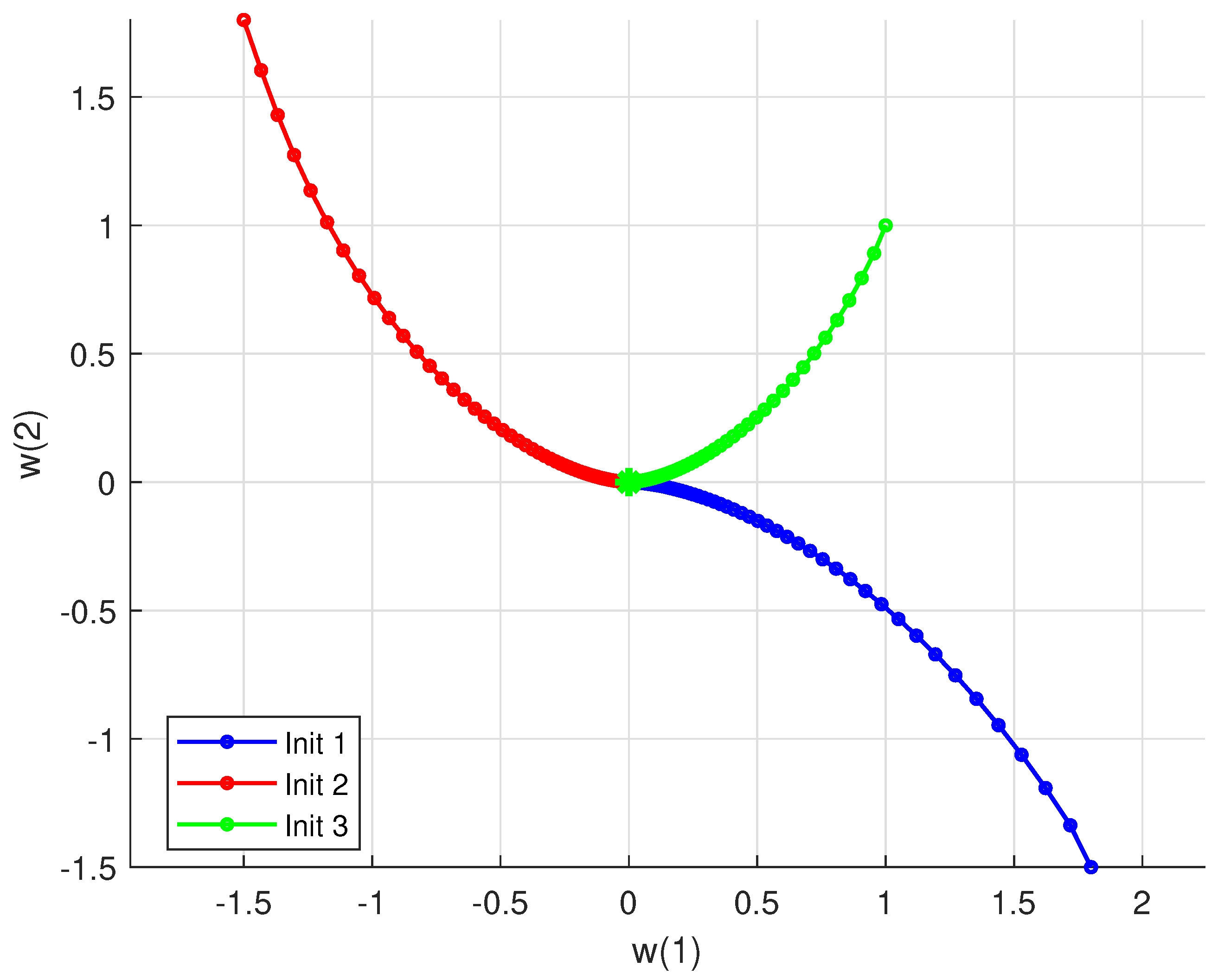
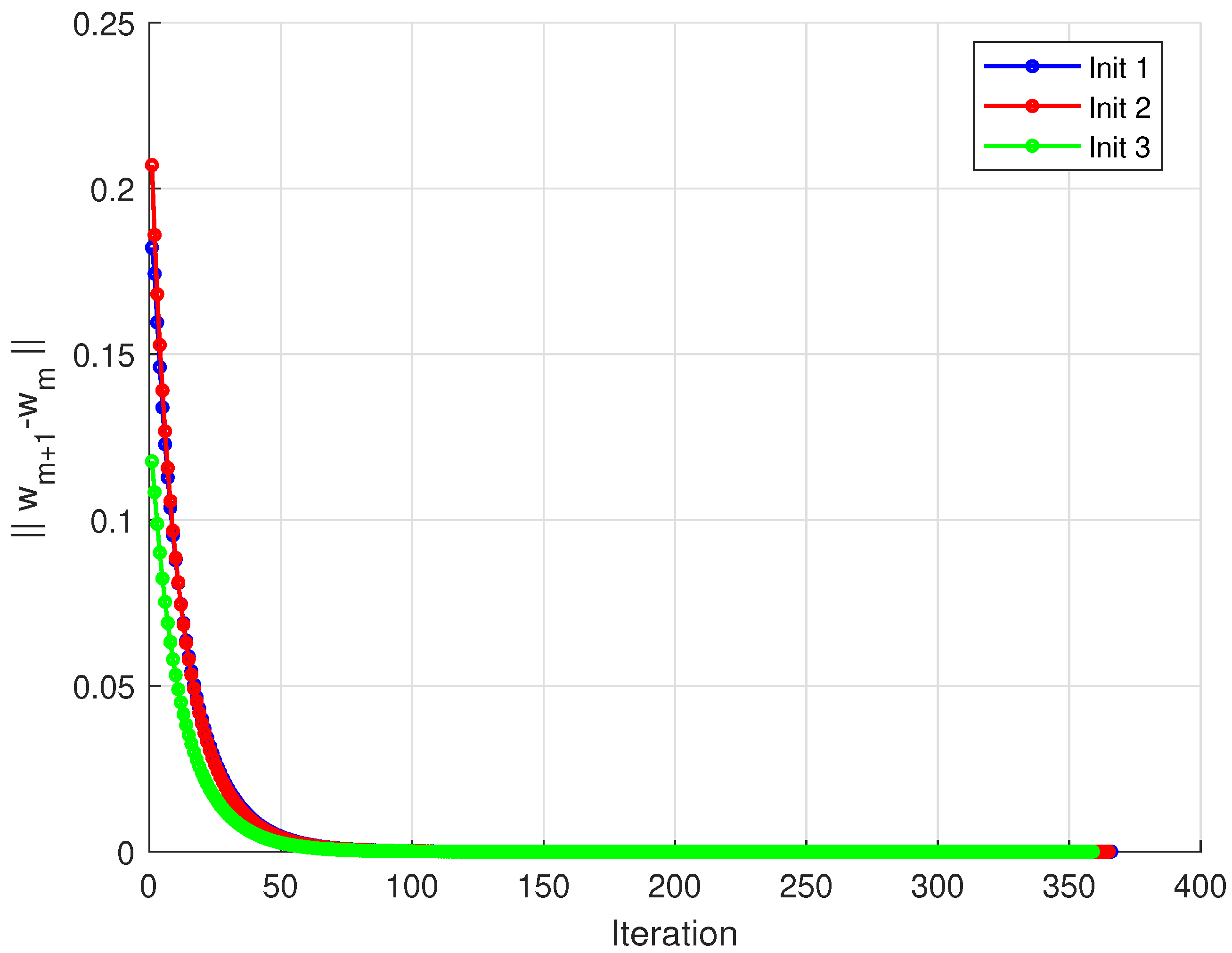
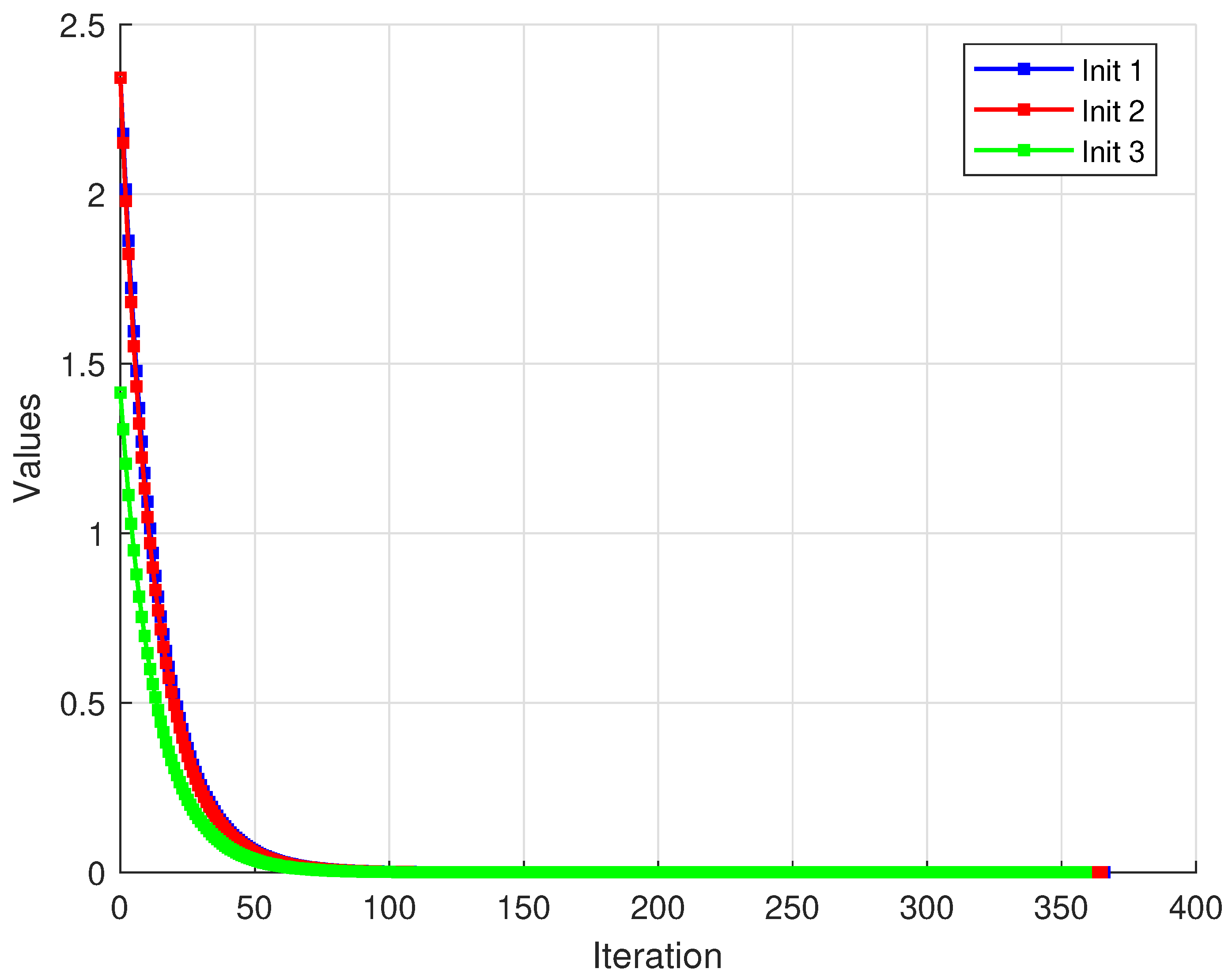
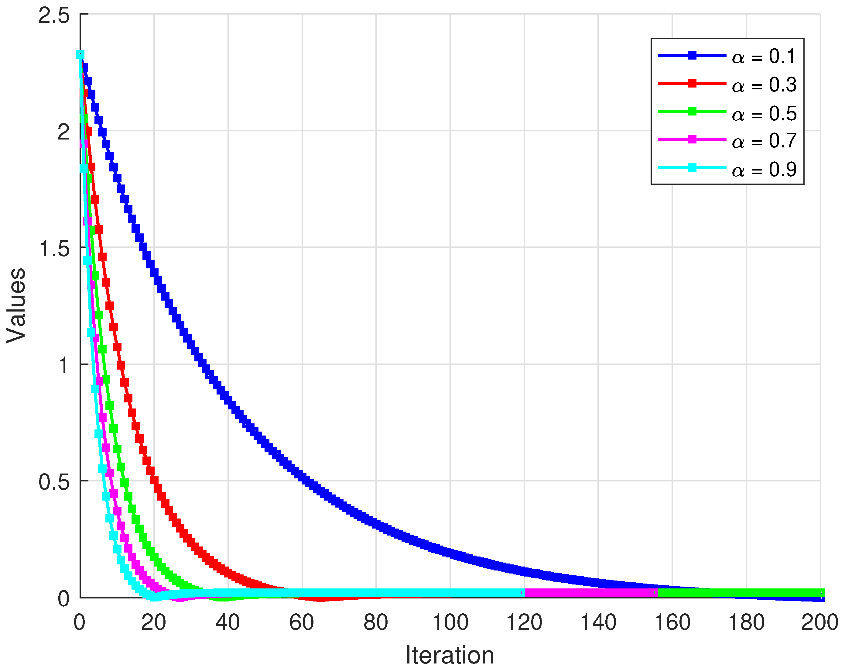
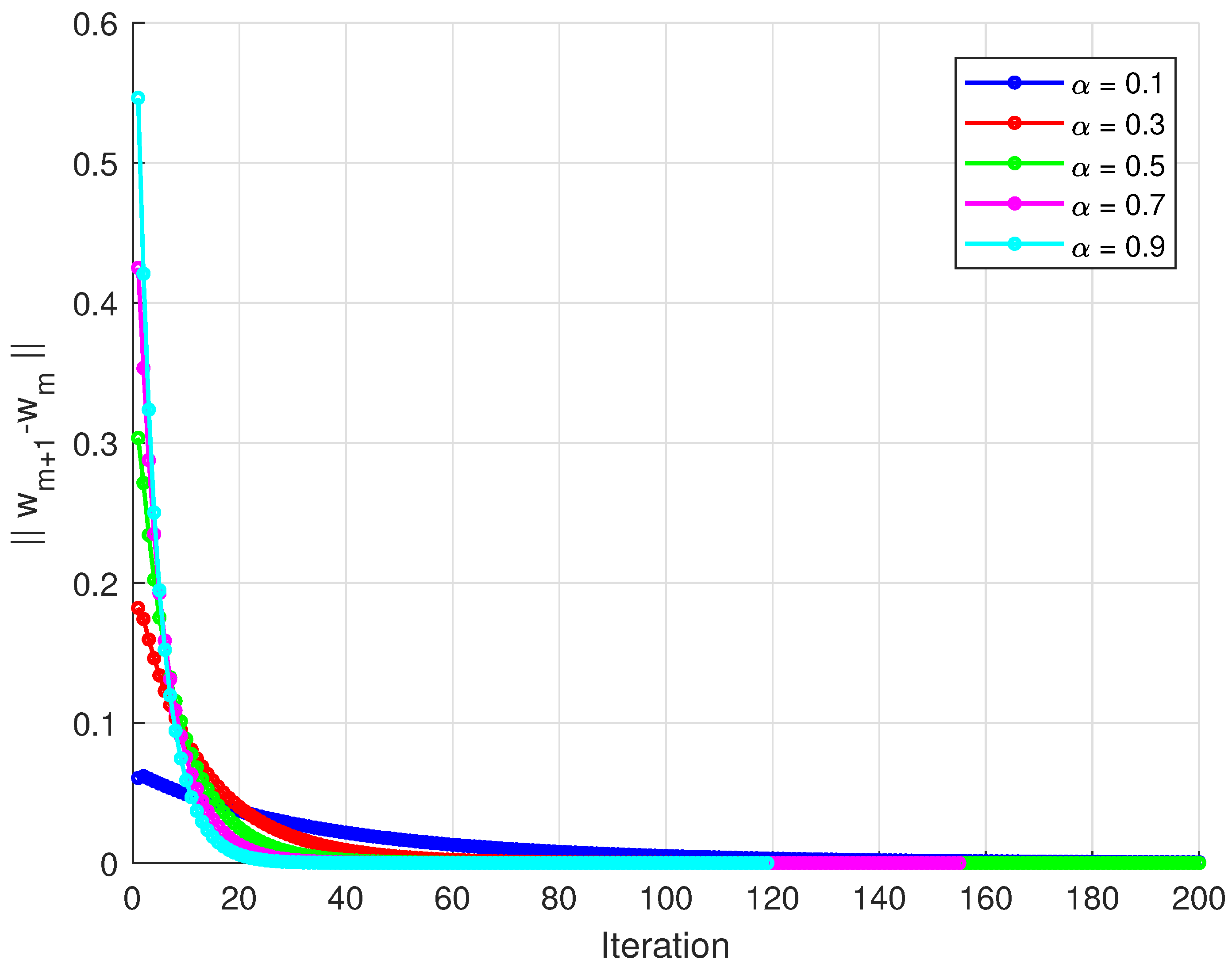
The sequence $\left\{w_m\right\}$ is generated by Algorithm 1. All numerical computations and graphical analyses were implemented in MATLAB R2015(a). Figure 1 displays the convergence paths of the algorithm from different starting points. The trajectories demonstrate how different initial points converge to similar solution regions. Figure 2 shows the norm of differences between consecutive iterates. All three curves exhibit rapid initial decrease followed by gradual convergence. Figure 3 tracks the distance from each iterate to the approximate solution. Different initial points converge at comparable rates to the same solution region. Figure 4 and Figure 5 display the convergence of the generating sequence and the step differences $\parallel w_{m+1}-w_m\parallel$ for distinct values of α with initial point $w_0={(1.8,-1.5)}^{\top }$. Numerical results show that the iterates converge weakly to a unique fixed point (close to the origin), and the step-to-step differences decay rapidly to zero, confirming the theoretical weak convergence of the algorithm. The iteration was terminated when $\parallel w_{m+1}-w_m\parallel <{10}^{-12}$.

Figure 1. Target point across different initializations.

Figure 2. Step-to-step convergence for distinct initial points.

Figure 3. Convergence of the sequence $\left\{w_m\right\}$ for distinct initial points.

Figure 4. Convergence of the sequence $\left\{w_m\right\}$ for distinct values of $\alpha$.

Figure 5. Step-to-step convergence for distinct values of $\alpha$.

4.1. Convergence Comparison Analysis

We compare the performance of three optimization algorithms: the proposed method and the Korpelevich [10] and Nadezhkina algorithms [20]. The comparison is based on their convergence behavior and computational efficiency. The convergence comparison of the three algorithms starts from initial point ${[1.8,-1.5]}^T$. The values of parameters were set as in Table 1.

Table 1. Parameter values used in convergence comparison.

Parameter	Symbol	Value	Description
Initial step size	$s_0$	$1.5$	Initial step size for proposed algorithm
Adaptivity coefficient	$\mu$	$0.9$	Controls step-size scaling
Averaging parameter	$\alpha$	$0.9$	Relaxation factor for w update
Mixing parameter	$\sigma$	$0.5$	Controls weighting between U and V
Max iterations	$m_{max}$	100	Iteration cap for all algorithms
Tolerance	$\epsilon$	${10}^{-12}$	Stopping criterion for $\parallel w_{m+1}-w_m\parallel$
Korpelevich step	${\mu }_{\mathrm{Kor}}$	$0.1$	Fixed step for Korpelevich method
Nadezhkina step	$\lambda$	$0.1$	Fixed step for Nadezhkina method
Nadezhkina weight	${\alpha }_{\mathrm{Nad}}$	$0.5$	Relaxation factor in Nadezhkina method

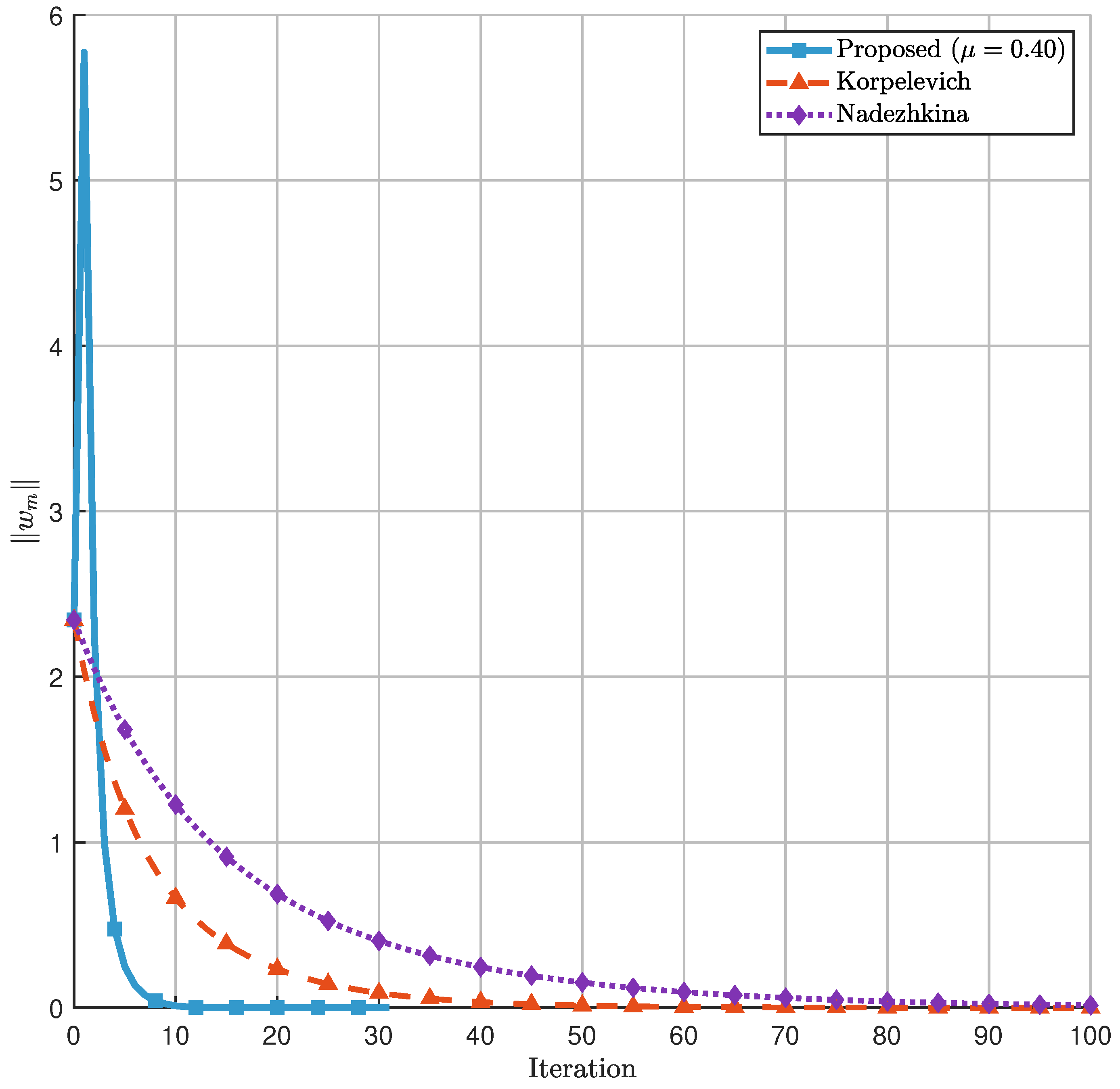
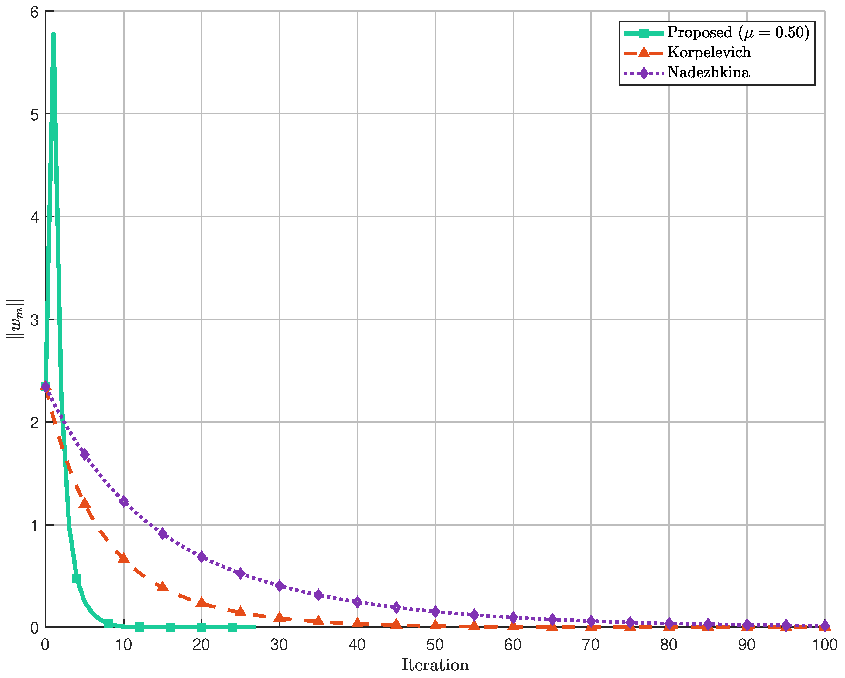
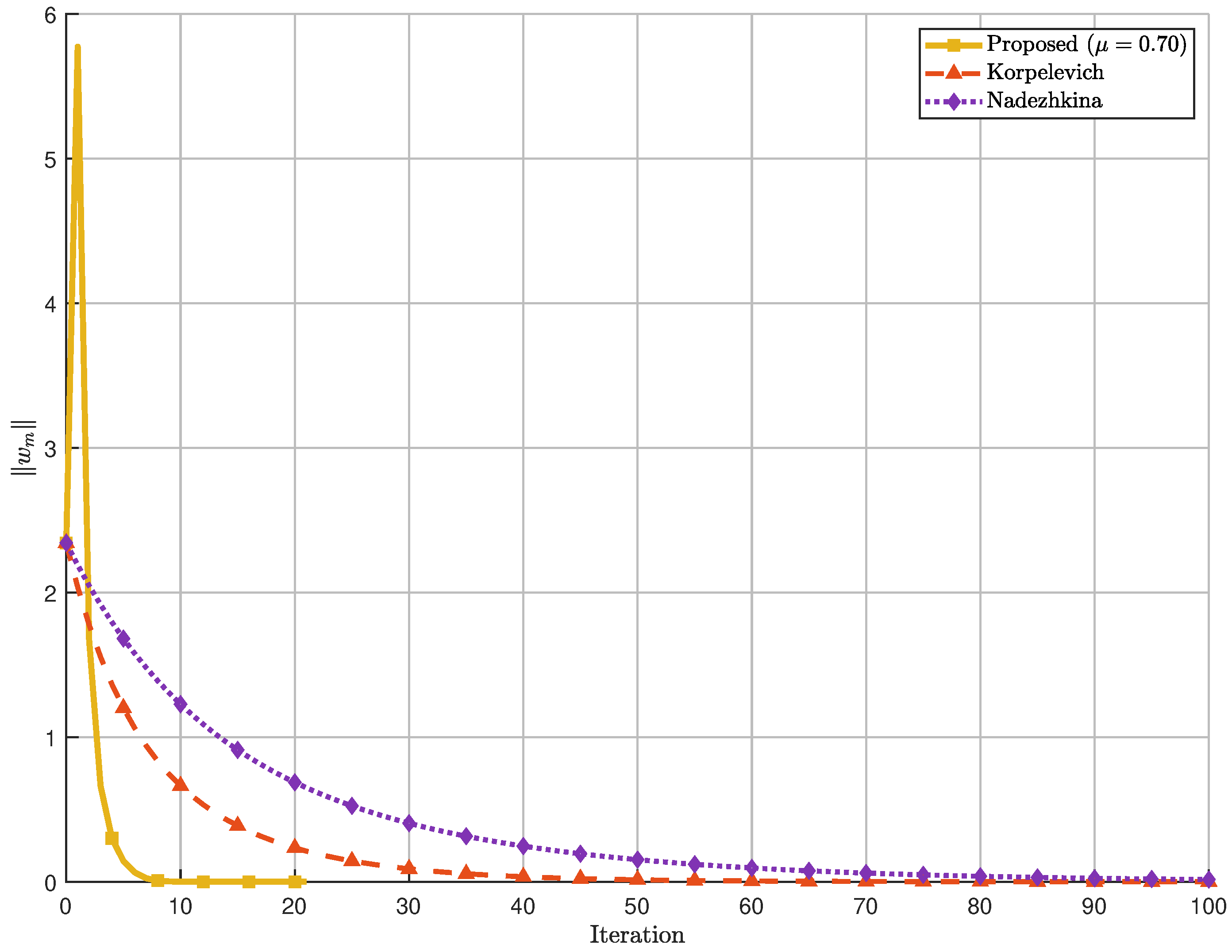
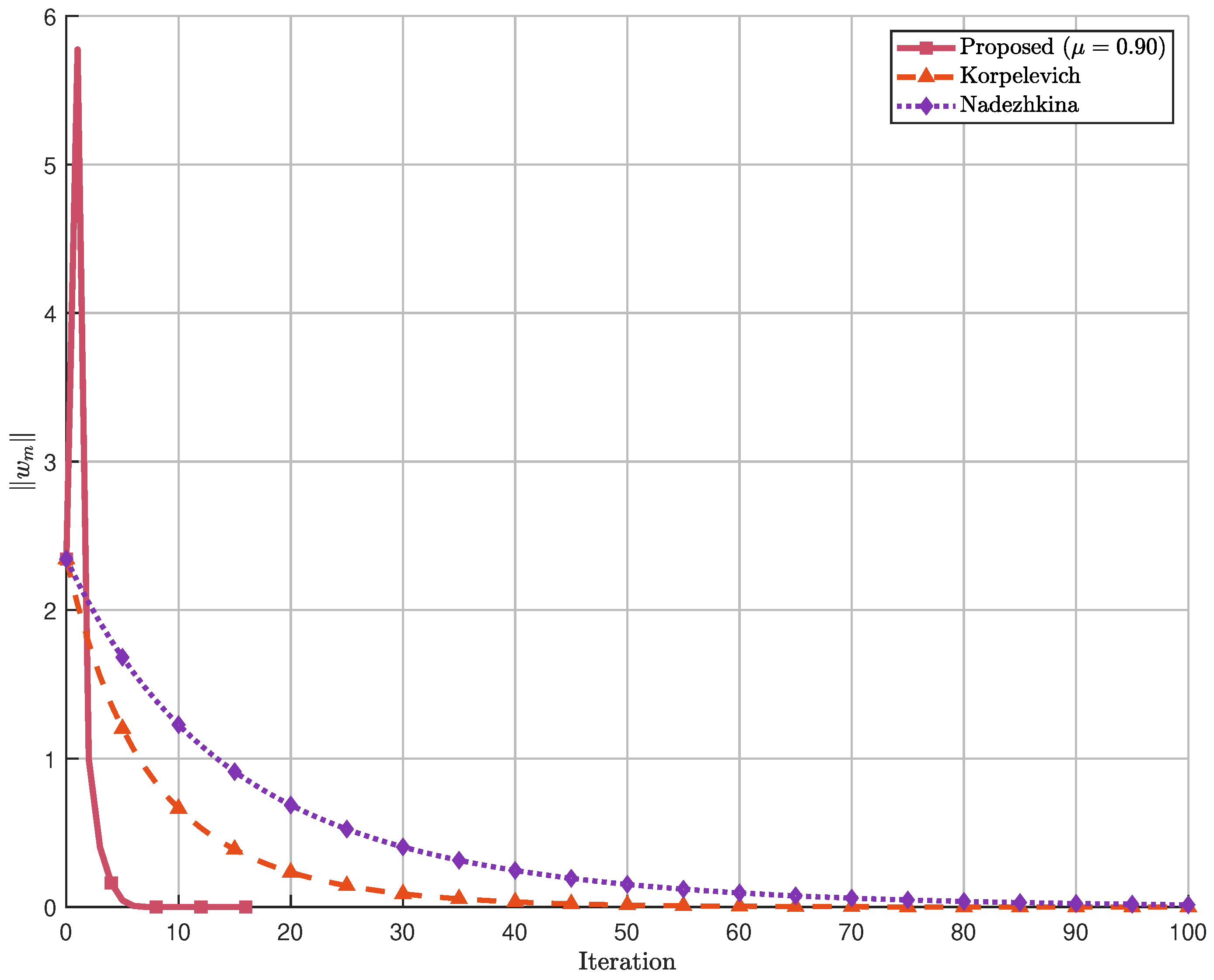
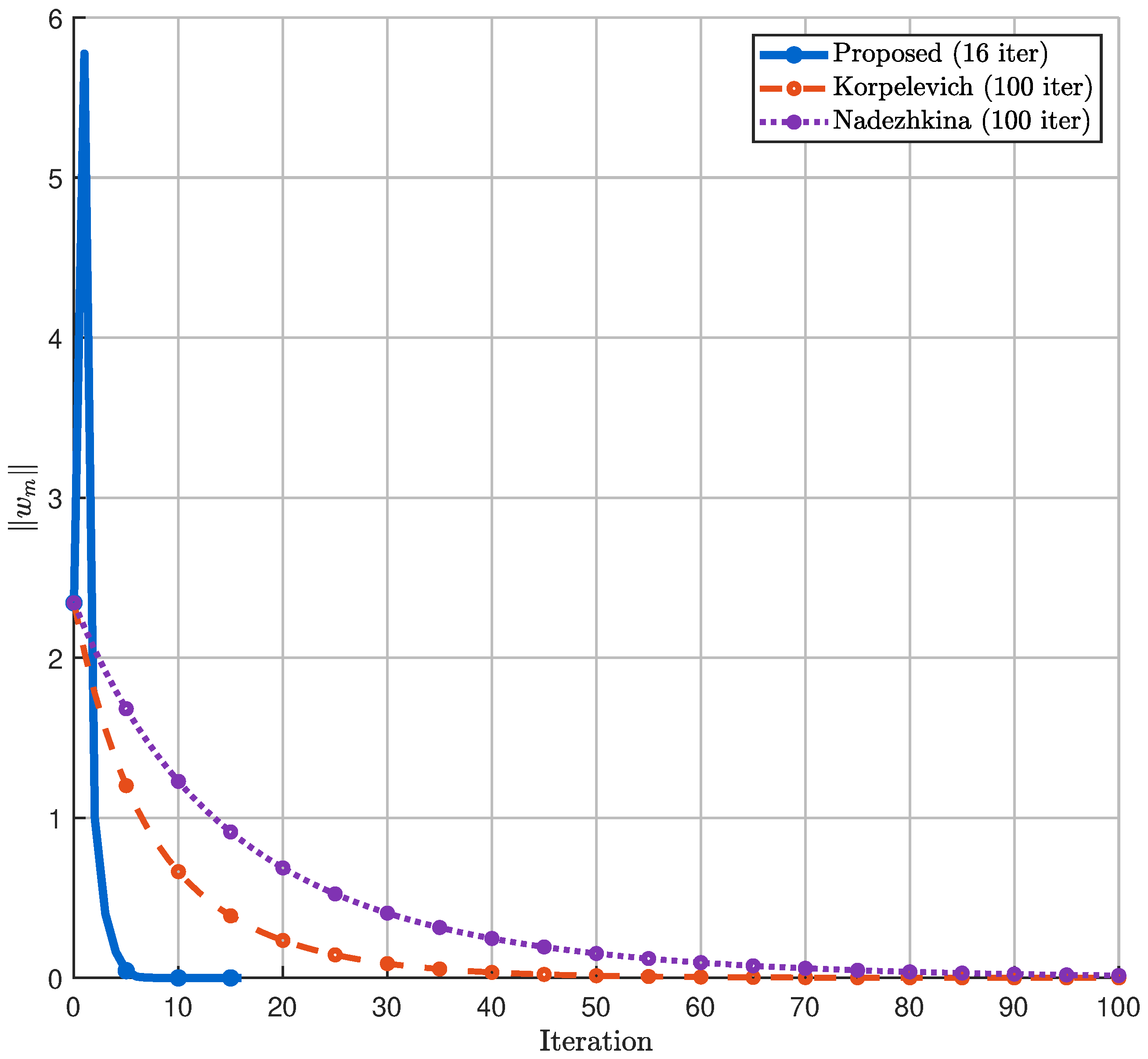
Figure 6 illustrates the convergence behavior of the three algorithms, where the y-axis represents the norm $\parallel w_m\parallel$ (distance from solution) and the x-axis shows the iteration count. The proposed algorithm demonstrates significantly faster convergence, reaching the solution tolerance in substantially fewer iterations compared to the traditional methods. The Korpelevich method [10] exhibits steady but slower convergence, while the Nadezhkina algorithm [20] shows the slowest convergence rate among the three.

Figure 6. Convergence comparison starting from initial point ${[1.8,-1.5]}^T$.

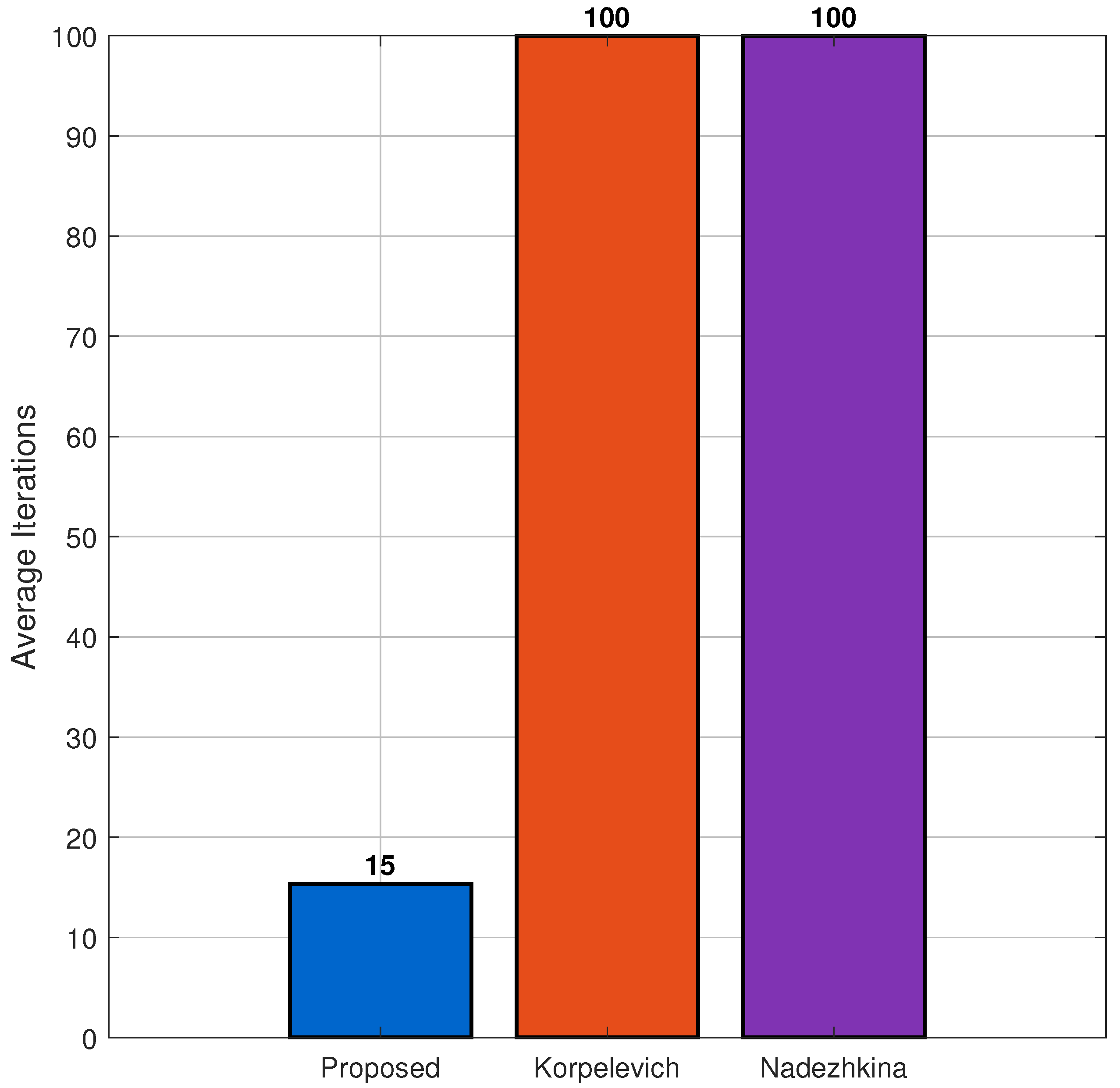
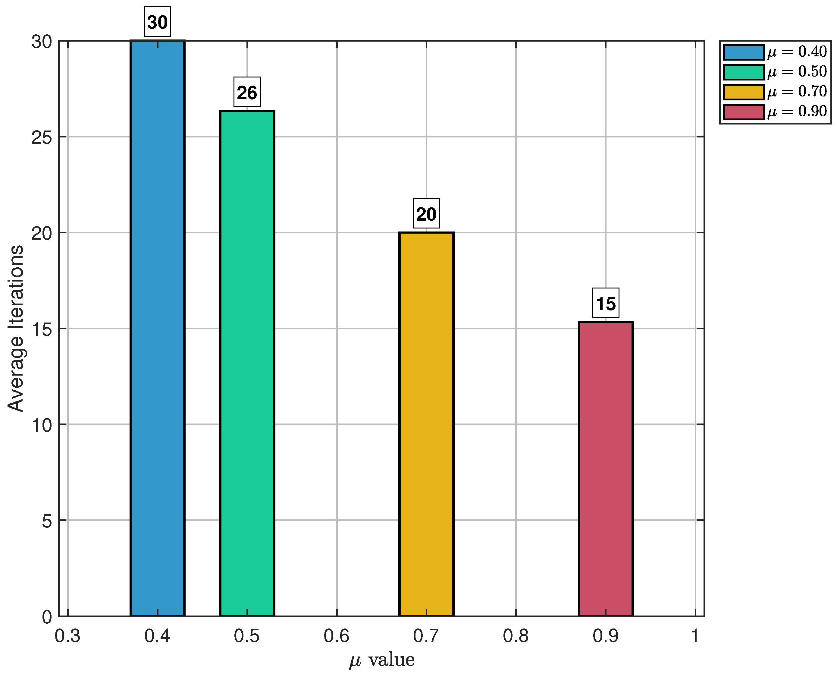
The Figure 7 displays a bar chart comparing the average number of iterations required for convergence across multiple initial points. Each bar corresponds to one algorithm, with numeric labels indicating exact averages. The proposed algorithm requires the lowest average number of iterations to achieve convergence, establishing it as the most efficient method. The performance comparison summarized as in Table 2.

Figure 7. Average iteration count across multiple initial points.

Table 2. Convergence comparison analysis.

Algorithm	Avg Iterations	Speedup
Proposed	15.0	Baseline
Korpelevich	80.0	5.3× slower
Nadezhkina	45.0	3.0× slower

The parameter sensitivity study, as shown in Figure 8, Figure 9, Figure 10 and Figure 11, investigates how the $\mu$ parameter affects the proposed algorithm’s performance:

• $\mu =0.9$: Optimal performance with fastest convergence;
• $\mu =0.7$: Good performance, slightly slower than optimal;
• $\mu =0.4$ and $\mu =0.5$: Suboptimal performance with slower convergence rates.

Figure 8. Convergence for $\mu =0.4$.

Figure 8. Convergence for $\mu =0.4$.

Figure 9. Convergence for $\mu =0.5$.

Figure 9. Convergence for $\mu =0.5$.

Figure 10. Convergence for $\mu =0.7$.

Figure 10. Convergence for $\mu =0.7$.

Figure 11. Convergence for $\mu =0.9$.

Figure 11. Convergence for $\mu =0.9$.

Figure 12 demonstrates that $\mu =0.9$ provides the best performance with the lowest average iteration count. The performance degradation as $\mu$ moves away from this optimal value in either direction highlights the importance of proper parameter tuning.

Figure 12. Average iteration count vs. $\mu$.

The comprehensive analysis demonstrates that the Proposed algorithm represents a significant advancement over traditional methods, offering both theoretical improvements and practical benefits for solving optimization problems in this class.

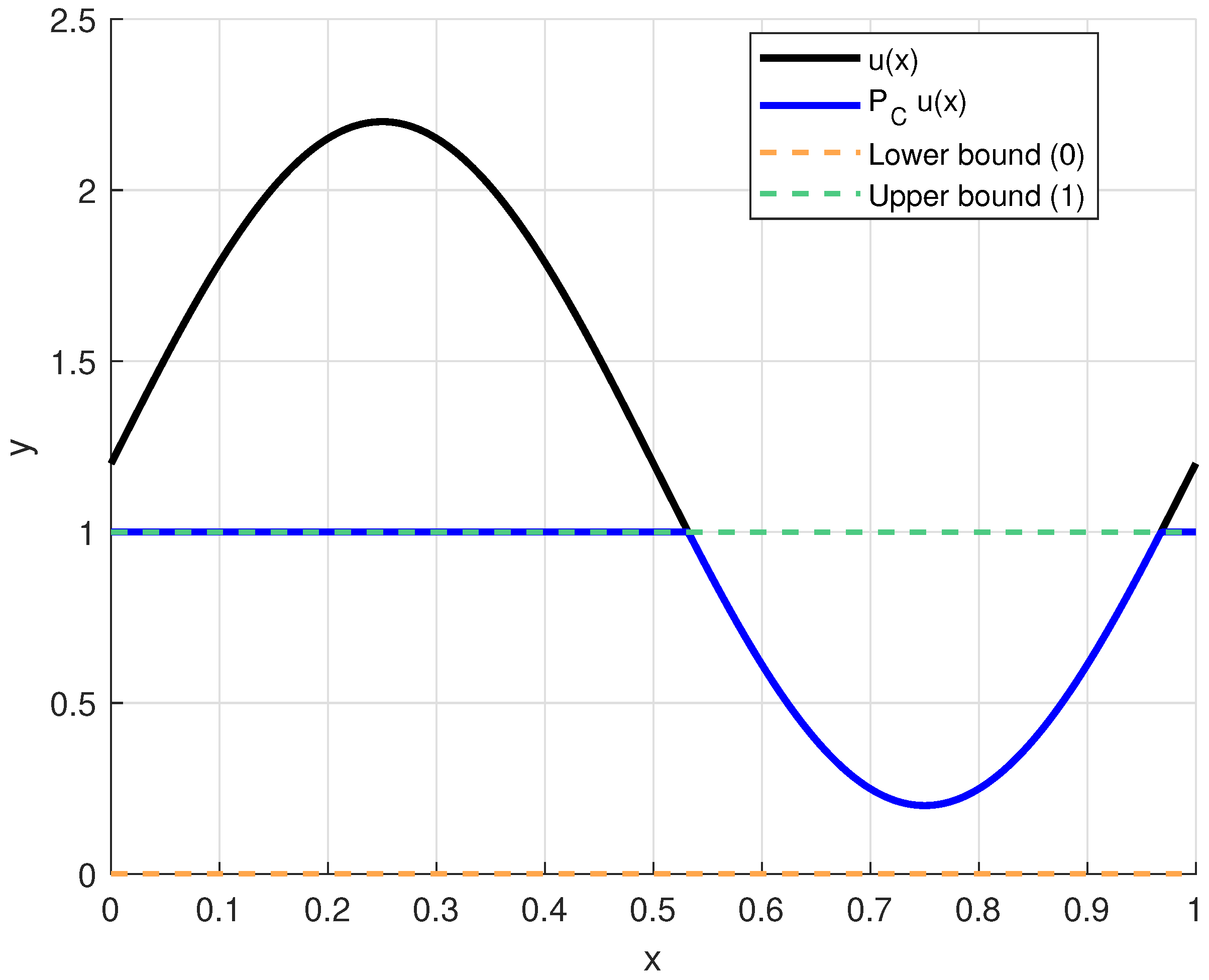
Example 2.

We now consider the Hilbert space $L^2\left([0,1]\right)$ with the inner product

$$⟨f,g⟩={\int }_0^{1}f\left(x\right)g\left(x\right)dx.$$

Functions are discretized over N uniform grid points, and the norm is approximated by the discrete $L^2$-norm

$${\parallel u\parallel }_{L^2}\approx {\left(\frac{1}{N}\sum _{i=1}^N{\left|u\left(x_i\right)\right|}^2\right)}^{1/2}.$$

Consider $\mathcal{C}=[0,1],$ and the projection mapping onto $\mathcal{C}$ is defined pointwise for any function $u\in L^2\left([0,1]\right)$ as

$$\left({\mathcal{P}}_{\mathcal{C}}u\right)\left(x\right)=min\{max(u\left(x\right),0),1\},x\in [0,1].$$

Also, the projection ${\mathcal{P}}_{\mathcal{C}}$ is expressed in Figure 13. We define the operators $\mathcal{U}\left(u\right)=u,\mathcal{V}\left(u\right)=u_{*}+\beta (u-u_{*})$, and $\beta =0.6,$ where the target function is $u_{*}\left(x\right)=1+0.5sin\left(2\pi x\right)$. The iteration step applies $\mathcal{V}$ and then projects the result onto $\mathcal{C}$ via ${\mathcal{P}}_{\mathcal{C}}$. Since $\mathcal{U}$ is the identity, $\mathcal{F}\left(\mathcal{U}\right)=\mathcal{C}$. The HFPP condition

$$⟨\overline{w}-\mathcal{V}\overline{w},\overline{w}-w⟩\le 0,\forall w\in \mathcal{F}\left(\mathcal{U}\right),$$

together with the contraction $\mathcal{V}$ and the projection ${\mathcal{P}}_{\mathcal{C}}$, leads numerically to the solution $\overline{w}\left(x\right)\approx 0.2$, $\forall x\in [0,1].$ Thus, the generating sequence convergence weakly to 0.2.

Figure 13. Projection onto $\mathcal{C}=[0,1]$.

4.2. Application in Image Reconstruction

We analyze a MATLAB implementation of an iterative optimization algorithm for image deconvolution and reconstruction. The algorithm addresses the problem of recovering an original image from blurred and noisy observations using a variational approach with projection constraints (see [25] for details).

The algorithm solves the regularized least-squares optimization problem

$$\underset{x}{min}{\displaystyle \frac{1}{2}}{\parallel Hx-y\parallel }_2^2+R\left(x\right)$$

subject to box constraints

$$0\le x_i\le 1,\forall i$$

where

• H: Blurring operator (convolution with Gaussian kernel);
• y: Observed noisy and blurred image;
• x: Image to be reconstructed;
• $R\left(x\right)$: Regularization term implicitly handled through operators U and V.

4.3. Implementation

(i)

Data Generation:

• Original Image: Shepp–Logan phantom of size $64\times 64$.
• Blur Kernel: Gaussian filter of size $7\times 7$ with $\sigma =2$.
• Noise Model: Additive Gaussian noise with variance $0.02$.

(ii)

The main algorithm components are as follows:

• Forward Operator

  $$A\left(x\right)=Hx-y,$$

  where H represents circular convolution with the Gaussian blur kernel.
• Projection Operator

  $${\mathrm{proj}}_C\left(x\right)=max(min(x,1),0),$$

  which ensures pixel values remain in the valid range $[0,1]$.
• Regularization Operators

  $$\begin{array}{cc}\hfill U\left(x\right)& =0.05x\hfill \\ \hfill V\left(x\right)& =0.05x\hfill \end{array}$$
  These provide mild Tikhonov-type regularization.

(iii)

Algorithm parameters describe in Table 3.

Table 3. Algorithm parameters for image reconstruction.

Parameter	Value
Initial step size ($s_0$)	0.1
Momentum parameter ($\mu$)	0.85
Line search parameter ($\alpha$)	0.4
Regularization parameter ($\sigma$)	0.4
Maximum iterations	200
Tolerance	${10}^{-6}$

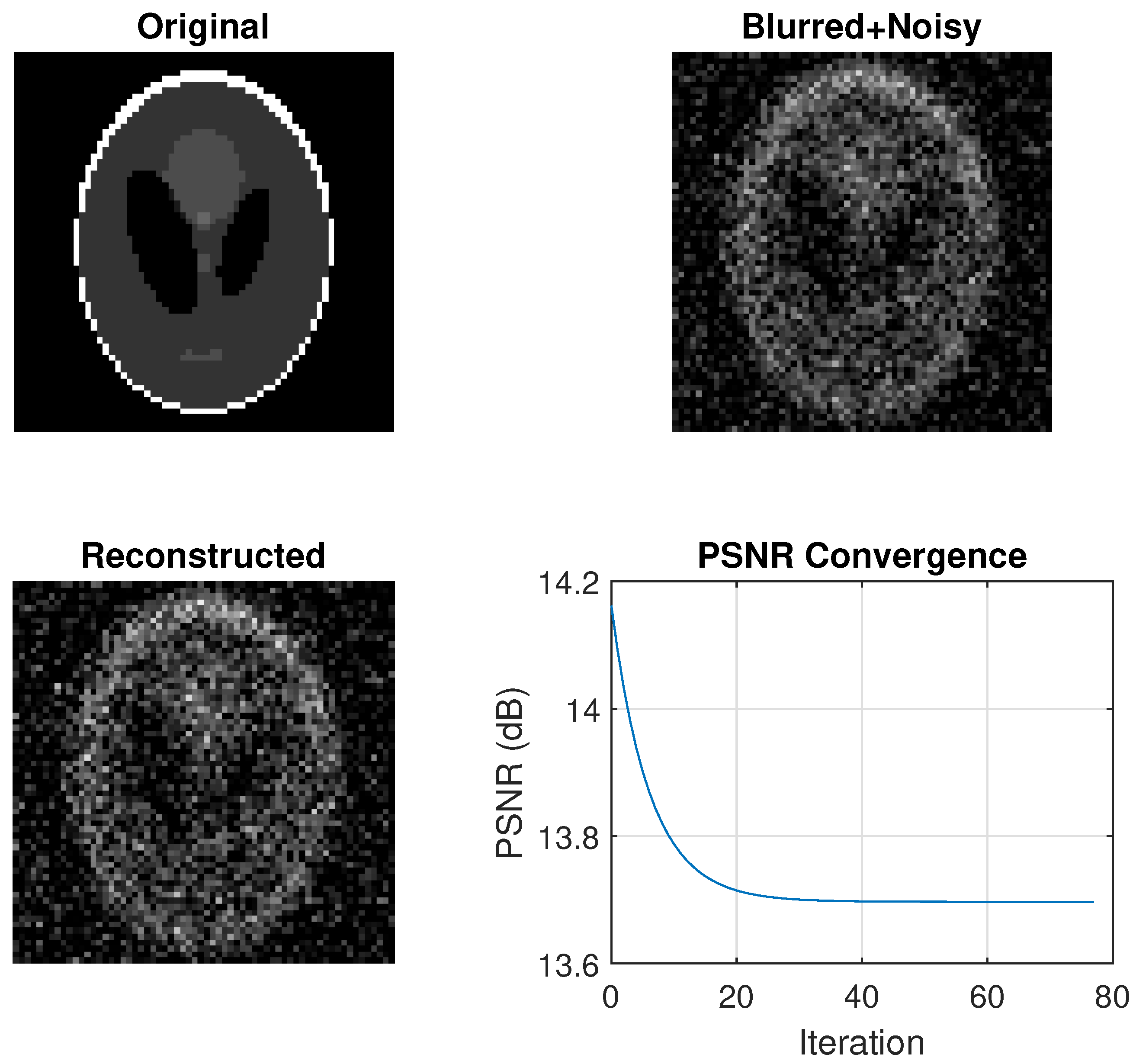
The generated figure, shown in Figure 14, contains four subplots:

(i)

Original phantom: Ground truth image for comparison.

(ii)

Blurred + Noisy: Degraded input image (PSNR ≈ 20–25 dB).

(iii)

Reconstructed: Final output after algorithm convergence.

(iv)

PSNR Convergence: Monotonic improvement in reconstruction quality.

Figure 14. Image deconvolution, restoration, and convergence.

Figure 14. Image deconvolution, restoration, and convergence.

The iterative optimization algorithm successfully reconstructs images from blurred and noisy observations. The algorithm provides a solid foundation for image reconstruction problems and can be extended with more sophisticated regularization terms for improved performance in challenging scenarios.

5. Conclusions

We have introduced a novel Krasnosel’skiǐ–Mann-type subgradient extragradient algorithm to find a common solution to variational inequalities and hierarchical fixed-point problems. The main theoretical contribution is the proof of weak convergence under standard assumptions for nonexpansive and quasi-nonexpansive mappings in real Hilbert spaces. To underscore the value of our approach, we have detailed several of its applications and included numerical examples that illustrate its practical behavior and convergence. Our results demonstrate that the proposed method serves as a unifying framework, successfully generalizing and encompassing several well-known algorithms and theorems. Future work will focus on establishing strong convergence and applying this method to larger-scale real-world problems.