


Abstract
Three-dimensional (3D) scene model retrieval has emerged as a novel and challenging area within content-based 3D model retrieval research. It plays an increasingly critical role in various domains, such as video games, film production, and immersive technologies, including virtual reality (VR), augmented reality (AR), and mixed reality (MR), where automated generation of 3D content is highly desirable. Despite their potential, the existing 3D scene retrieval techniques often overlook the rich semantic relationships among objects and between objects and their surrounding scenes. To address this gap, we introduce a comprehensive scene semantic tree that systematically encodes learned object occurrence probabilities within each scene category, capturing essential semantic information. Building upon this structure, we propose a novel semantics-driven image-based 3D scene retrieval method. The experimental evaluations show that the proposed approach effectively models scene semantics, enables more accurate similarity assessments between 3D scenes, and achieves substantial performance improvements. All the experimental results, along with the associated code and datasets, are available on the project website.
Keywords:
3D scene retrieval; semantics; semantic information; scene objects; semantic segmentation; deep learning MSC:
68U05; 68T45; 68T07
1. Introduction
Three-dimensional (3D) models consist of 3D data (typically a list of vertices and faces) to represent 3D objects. Three-dimensional models are widely used in several fields, such as industry product design, visualization and entertainment, 3D modeling, rendering, and animation. In recent years, the number of 3D models has continued to increase drastically, triggering urgent research tasks and generating various research interests in developing effective and efficient 3D shape retrieval algorithms for related applications. Given a query that is often a 2D sketch/image or a 3D model, content-based 3D model retrieval serves to retrieve relevant 3D models (typically only single-object models) from the same category as the query and then rank them in the front part of the rank list as much as possible while at the same time pushing irrelevant 3D models to the back of the rank list. Effectiveness, efficiency, and scalability are the three most important performance measures/evaluation criteria, which can be measured by a set of performance metrics commonly used in the field of information retrieval.
Three-dimensional scene model retrieval [1] is a new research direction in the field of 3D model retrieval. It aims to retrieve man-made 3D scene models given a user’s hand-drawn 2D scene sketch or a 2D scene image usually captured by a camera. It has a vast array of important practical applications, including 3D game/movie production, virtual, augmented, and mixed reality (technologies that blend the physical and digital (virtual) worlds to varying degrees: VR creates fully simulated environments, AR adds digital objects to the real world, and MR lets users interact with both real and virtual things at the same time), metaverse, and 3D entertainment, where automatic 3D content production is very important and in demand. For typical 3D model retrieval, a query sketch/image/model or a target 3D model only contains a single object. However, for 3D scene retrieval, a query scene sketch/image/model or a target 3D scene model has multiple objects that may be occluded by each other, which makes the research topic more challenging. In the meantime, it also contains a great deal of semantic information, such as object–object and object–scene statistical relationships. Taking advantage of such already available, helpful, and important semantic information will have a significant positive impact on 3D scene retrieval performance. However, according to our knowledge, most such semantic information has been totally ignored or not been fully explored and utilized in the current available 3D scene retrieval algorithms [1]. In short, 3D scene model retrieval is a useful and promising but more challenging research topic that deserves further exploration.
Motivated by the above facts, to further boost the performance of 3D scene retrieval, we propose a semantics-driven image-based 3D scene retrieval framework. In this paper, we propose a comprehensive and novel semantic tree-based 3D scene retrieval framework, as illustrated in Figure 1. Given a 2D query image and a dataset of 3D scene models, we first construct a scene semantic tree (SST) in the first two stages of our retrieval algorithm. Stage 1 (S1 in Figure 1): Build a scene semantic tree based on the semantic ontology in WordNet [2]. Then, classify collected 2D scene images and 3D scene models into certain nodes of the tree according to their semantic classification/label information (i.e., semantic concepts or names). Stage 2 (S2–S4): Next, for each scene category, by utilizing scene object detection and deep learning techniques, we learn its scene semantic information (SSI), which automatically encodes its scene object occurrence probabilities. Stage 3 (S5): Finally, a semantics-driven image-based 3D scene retrieval approach is developed by leveraging the established scene semantic tree in combination with a scene classification and majority voting strategy. The experiments demonstrate that our semantics-based approach is capable of effectively capturing the semantic information of 2D scene images and 3D scene models, accurately measuring their similarities, and therefore greatly enhancing the retrieval performance.
Figure 1.
Semantics-driven 2D scene image-based 3D scene model retrieval framework. S1, S2, …, S5, correspond to the five steps in Section 3 accordingly. is used to represent the object occurrence distribution of each scene category: O means an object class, while p is its occurrence probability in that scene (adapted with permission from [3], IEEE, 2020).
This project is an extension of our initially proposed method named the deep random field (DRF) model [3] published at a conference. The main differences lie in their purposes (our method is designed for retrieval, while DRF is for recognition), loss function definitions, as well as the resulting significant differences in retrieval performance. A detailed review of DRF is provided in Section 2.2. A comprehensive comparison between DRF and the joint loss-based retrieval method (JLR) proposed in this paper can be found in Section 3.5 and Section 4.3.
To the best of our knowledge, this project is the first attempt to explore matching between 2D scene images and 3D scenes at the semantic level using a tree structure, and to develop a comprehensive framework to perform 3D scene retrieval. The main contributions of the work can be summarized as follows:
- A large comprehensive scene semantic tree is created based on WordNet. It is a pioneering work to lead this semantics-driven 3D scene retrieval research, and it also provides a very useful scene semantic infrastructur for many related applications.
- A novel and effective semantic tree-based 3D scene retrieval framework (see Figure 1) is proposed that greatly enhances the 2D scene image-based 3D scene retrieval performance according to our experimental results.
The project will accelerate the speed of applying 3D scene retrieval techniques in related large-scale applications by providing an infrastructure to perform information search at the semantic level, like Google. This is because efficient and accurate large-scale 3D scene retrieval algorithms are important for several related applications that involve 3D scene models. Therefore, the project will have a direct broad impact on many related promising applications.
2. Related Work
Semantic 3D scene retrieval algorithms involve three basic components: scene processing, semantic information representation, and evaluation. Therefore, in this section, in chronological order, we will review the currently most popular and dominating scene processing techniques: deep learning-based (Section 2.1), typical semantic information representations in 2D/3D scene understanding (Section 2.2), and related 2D/3D scene benchmarks (Section 2.3).
2.1. Deep Learning Technique-Based Scene Processing
YOLO-based scene object detection. Redmon et al. proposed a YOLO (v1 [4], v2 [5], and v3 [6]) system that can be used for image or video object detection. It is a state-of-the-art real-time one-stage end-to-end object detection system. It has an advantage when compared with other object detection techniques: detection speed is fast while simultaneously maintaining high accuracy. Compared to YOLOv1 and YOLOv2, YOLOv3 demonstrates greatly enhanced performance: (1) multi-label prediction, adopting binary cross-entropy loss (logistic classifier) instead of softmax to solve the multi-label problem (e.g., man and person); (2) small-object detection: solving the small-object detection problem by using shortcut connections; and (3) feature extractor network: the backbone net structure has been improved from Darknet-19 in v2 to Darknet-53 with deeper layers. YOLOv3 supports custom retraining and fine-tuning workflows, allowing us to add new classes without starting from scratch. For example, it enables us to freeze early layers while only modifying the last detection layers to match our desired number of classes to train on our custom data. Considering the above factors, in this paper, we adopt YOLOv3 for the task of object occurrence prediction in Section 3.
In 2018, He et al. [7] presented a triplet center loss (TCL)-based 3D object retrieval method, whose loss function contains two parts: triplet loss and center loss. Compared with the traditional softmax loss function, which is usually utilized for 3D shape classification, the triplet center loss function is able to learn more discriminative features for 3D shape retrieval. Based on the triplet center loss, they learned an embedding space where the distance between samples of the same class is less than the distance between samples of different classes. In our paper, we adopt the TCL loss function as one component of the loss function of our model.
In 2020, Caglayan et al. [8] proposed a two-stage object and scene recognition framework, which can recognize scenes from RGB-D images captured by RGB-D sensors. The first stage is a pretrained CNN model that can extract multi-level visual features. The second stage utilizes multiple random recursive neural networks (RNNs) to map the extracted features into high-level representations. In addition, they extended the idea of randomness in RCNNs and proposed a randomized pooling scheme to improve the recognition accuracy.
Due to the fact that some acquired 3D scene data may be incomplete during the process of 3D capturing, e.g., objects occlude each other, views are insufficient while capturing, etc., in 2020, Wang et al. [9] proposed an octree-based CNN (O-CNN) network with a U-Net-like structure to complete and clean such defective 3D scene data. This network supports very deep architectures (e.g., up to 70 layers) and contains an output-guided skip connection, which can preserve the current input geometry and learn new geometry from the input data. The results demonstrate improved prediction accuracy compared to state-of-the-art approaches.
In 2021, Murez et al. [10] presented an end-to-end method for 3D scene reconstruction. Unlike traditional 3D scene reconstruction approaches, which often utilize an intermediate representation of depth maps for predicting truncated signed distance function (TSDF) values [11], their reconstruction approach can predict the TSDF directly without requiring depth map inputs: one CNN is used first to extract features from each RGB image, and then another CNN is used to refine the features and predict the TSDF values. In addition, their model obtains semantic segmentation label information with low computation. An evaluation on the ScanNet [12] dataset demonstrates its better performance than the state-of-the-art baselines.
To handle remote sensing (RS) image scene classification, Xu et al. [13] proposed a dual-branch convolutional neural network (CNN) named Attention Consistent Network (ACNet), focusing on both global features and local details through spatial rotation and attention mechanisms. ACNet employs a Siamese-like structure to minimize/maximize feature distances between images of the same/different classes and utilizes attention techniques to highlight salient features for accurate classification. The effectiveness of ACNet is validated across three popular RS scene datasets, demonstrating its ability in enhancing RS image classification by addressing both global and local feature representation challenges.
In 2023, Jiang et al. [14] proposed a dual-task model leveraging PointNet++ [15] for indoor scene recognition and semantic segmentation, addressing the challenges posed by 2D data limitations and the complexity of indoor environments. By integrating multi-dimensional labels, task state control, and a shared feature layer, the model achieved good accuracy in both scene recognition (82.4%) and semantic segmentation (98.9%). Through the application of scene-element rules, it also corrects recognition errors, offering an approach to understand indoor spaces with 3D point cloud data.
In 2024, Naseer et al. [16] proposed a multi-step scene recognition framework that exploits depth information to achieve real-time scene understanding for robots. Their method first applies a U-Net-based semantic segmentation network to segment multiple objects in the scene and then extracts entropy-based features from the segmented regions. These features are optimized and fed into a CNN classifier to recognize the scene. By tightly integrating depth preprocessing, deep-learning segmentation, and feature-engineering-based classification, their approach achieved better performance than several existing systems and showed that depth data can be effectively leveraged to improve 3D scene comprehension.
Because scene recognition often faces high inter-class similarity and most object-assisted methods are too costly for edge devices, in 2024, Song et al. [17] proposed a semantic knowledge-based similarity prototype that guides scene recognition without adding extra parameters or inference cost. They first summarized scene semantics into class-level representations and used these to build a prototype describing how scene classes relate to one another. This prototype is then used in two ways: gradient label softening (to provide smoother supervision) and batch-level contrastive loss (to enforce similarity/dissimilarity in each batch). Experiments on MIT-67 [18], SUN [19], and Places [20] show consistent improvements.
In 2024, Sagar et al. [21] introduced the MSA R-CNN framework for remote sensing object detection and scene understanding. The model integrates a super multiscale feature extraction network (SMENet) to enhance feature extraction from high-resolution images, along with an adaptive dynamic inner lateral (ADIL) module to mitigate information loss in feature pyramid networks and a distributed lightweight attention module (DLAM) to refine feature representation. Although the approach showed high accuracy, the authors acknowledged its computational complexity and emphasized the need for future work to reduce model cost while maintaining robust detection capabilities.
In 2024, Ajantha et al. [22] presented a survey of YOLO-based object detection models, tracing their evolution from the initial release in 2015 to the latest version in 2023. The review highlighted YOLO’s strengths in delivering high detection accuracy and fast inference compared with two-stage detectors, making it well-suited for real-time applications. The authors also identified ongoing challenges, such as detecting unseen objects and operating in complex environments, and suggested that integrating advanced architectures like ConvNeXt [23] into YOLO could further enhance feature extraction and overall detection performance.
In 2025, Trigka et al. [24] published a comprehensive survey on machine learning and deep learning techniques for object detection, analyzing their evolution, performance, and limitations. The study underscored the contributions of deep learning architectures, particularly neural networks, in advancing detection accuracy, robustness, and real-time applicability across domains, such as autonomous driving and medical imaging. It also examined challenges, including occlusions, varying object scales, and the demand for faster processing, while emphasizing the importance of emerging architectures, such as Transformers and semi-supervised methods. Overall, the survey concluded that, while ML- and DL-based object detection systems have become highly effective, further innovation is required to overcome the existing barriers and enhance efficiency and interpretability.
2.2. Semantics-Based 3D Scene Understanding
WordNet-based semantics-driven 3D scene understanding. As a well-known lexical database, WordNet [2] has been utilized in different semantics-driven multimedia applications. WordNet is composed of concepts/synsets, which are represented by a set of synonyms. WordNet is tree-structured, and each node of the tree comprises a set of words, each with one or more senses (meanings). Each sense (meaning) has its synset, and three relationships (hypernyms/hyponyms (IS_A relation), holonyms (MEMBER_OF relation), and meronyms (PART_OF relation)) are used to represent the relationships among a set of words. Based on WordNet, researchers have developed several semantic similarity metrics, such as LCH (Leacock and Chodorow [25]), WUP (Wu and Palmer [26]), and path-based similarity measures [27], as well as some semantic relatedness metrics, including HSO (Hirst and St-Onge [28]), Lesk (Banerjee and Pedersen [29]), and Vector (Patwardhan [30]). Some other semantic relatedness and similarity approaches can be found in Patwardhan et al. [31] and Pedersen et al. [32]. With the available semantic hierarchy for concepts and related semantic measures, WordNet has been applied to building benchmarks for different visual understanding tasks [33], including 2D object images (i.e., ImageNet [34]), 3D models (i.e., ShapeNet [35]), 2D scene images (i.e., Places [20]), and videos (activity-level) (i.e., [36]). In addition, it is useful as a knowledge graph (like Freebase [37] for generic human knowledge and GeneOntology [38] for biology). It is also useful for natural language understanding [39] and building its connection to visual understanding, such as in Visual Genome [40].
WordNet is one of the most widely used lexical databases for measuring semantic similarity between words. Owing to its comprehensive coverage and well-defined ontology, WordNet has become a foundational resource in numerous natural language processing applications, including word sense disambiguation, information retrieval, and semantic analysis. Therefore, we also adopt WordNet in our approach to build our scene semantic tree, and extract its scene semantic information.
In 2019, Armeni et al. [41] presented a semi-automatic framework to construct a 3D scene graph, which can carry various types of semantic information (e.g., object labels, scene categories, material types, etc.) available in a 3D scene. This 3D scene graph contains four layers, which can represent the semantic information, camera position, and 3D spatial relations (e.g., occlusion and relative volume). The construction of such 3D scene graphs is usually conducted manually, so the involved labor is heavy. This framework can mitigate this problem by utilizing existing learning methods (e.g., Mask R-CNN [42]) and improving them in two ways: (1) framing, which samples query images from panoramas in order to enhance the performance of 2D object detectors; and (2) multi-view consistency, which addresses issues originating from 2D object detection of different camera positions.
In 2024, Lv et al. [43] presented SGFormer, a semantic graph Transformer for point cloud-based 3D scene graph generation. Unlike earlier Graph Convolutional Network (GCN)-based approaches that suffer from over-smoothing and can only pass information to nearby nodes, SGFormer is built on Transformer layers so that global relationships in the scene can be modeled directly. The authors designed two task-specific components: a graph embedding layer, which makes better use of global edge information while keeping computation reasonable, and a semantic injection layer, which injects linguistic knowledge from large language models (e.g., ChatGPT) to enrich the visual features of objects.
As our prior related work, in 2020, we proposed a semantic-tree based 3D scene model recognition approach [3]. The semantic tree is a hierarchical directed graph of semantic concepts (i.e., scene categorical labels/classes) and objects (i.e., scene sketches/images/models). The graph adopts the structure of the WordNet [2], which has a hierarchical structure of concepts/synsets. The semantic tree-based approach utilizes the semantic relatedness information between each scene object’s label and the corresponding 3D scene’s label. The semantic relatedness information was incorporated in the definition of the loss function of our CNN model. After employing the scene semantic information, our method achieved a significant performance increase of 12.3% in scene recognition accuracy on the testing dataset compared to the same method without using the semantic information.
In 2020, Huang et al. [44] proposed a multitask learning-based [45] 3D indoor scene recognition method. This method classifies 3D indoor scenes based on 3D point cloud or voxel data instead of 2D images. They also incorporated the semantic object label information during the 3D indoor scene recognition process. By combing the geometric and object label information of a scene, the multitask method achieved 90.3% recognition accuracy on the ScanNet [12] dataset.
In 2020, Li et al. [46] proposed an anisotropic convolutional network (AIC-Net) for 3D semantic scene completion. This network overcomes the limitations existing in standard 3D convolution methods, which utilize a fixed 3D receptive field. The AIC-Net utilizes an anisotropic 3D receptive field and decomposes the 3D convolution into three 1D convolutions. These stacked 1D convolutions improve the voxel-wise modeling performance by adaptively determining the kernel size for each 1D convolution. Therefore, they allow the network to more flexibly control the receptive field of each voxel. In addition, the core module of the AIC-Net can be used as a plug-in for other existing networks. Wald et al. [47] proposed to learn a scene graph to understand the relationships among the entities in the point cloud of a scene, as well as its application in 2D–3D or 3D–3D matching.
In 2020, Ku et al. [48] organized a semantic object segmentation contest track based on collected 3D point cloud data of street scenes, which were annotated into five classes (building, ground, car, vegetation, and pole), in the 2020 Eurographics Shape Retrieval Contest (SHREC). This contest was challenging due to the fact that, by utilizing LiDAR scanners, the captured raw large-scale 3D point cloud data contained tremendous points and were usually non-uniformly distributed. The running results of a state-of-the-art deep learning-based method named PointNet++ [15] were provided as the baseline for the semantic segmentation task. Four (three learning-based and one non-learning-based) methods were contributed by the participants, and all four methods outperformed the baseline method. Specifically, one learning-based approach achieved the best performance, which proves the trend, especially for this challenging task with unbalanced data.
In 2023, Chen et al. [49] introduced CLIP2Scene, a framework that transfers knowledge from 2D image-text pretrained models to a 3D point cloud network. The method employs a semantics-driven cross-modal contrastive learning approach, utilizing CLIP’s text semantics to select positive and negative point samples, and enforcing consistency between temporally coherent point cloud features and their corresponding image features. Experiments on datasets like SemanticKITTI, nuScenes, and ScanNet demonstrate that CLIP2Scene achieves annotation-free 3D semantic segmentation, outperforming other self-supervised methods when fine-tuned with limited labeled data. This work highlights the potential of leveraging 2D pretrained models for label-efficient 3D scene understanding.
In 2024, Zemskova and Yudin [50] introduced 3DGraphLLM, a method that combines semantic graphs and large language models (LLMs) for 3D scene understanding. The approach leverages scene graphs to model spatial relationships between objects and utilizes LLMs to enhance the understanding of complex 3D scenes. Further, 3DGraphLLM has demonstrated state-of-the-art results in 3D referred object grounding and scene captioning tasks.
In 2025, Deng et al. [51] introduced an object detection-based visual SLAM optimization method for dynamic scenes, addressing the limitations of traditional static-environment assumptions. The proposed RGB-D visual SLAM system incorporated a parallel semantic thread and a dynamic feature rejection module to effectively handle moving objects while leveraging both semantic and geometric cues. Dense point cloud maps were constructed using depth data and voxel grid filtering, thereby enhancing robustness and visualization quality compared to sparse metric maps. Experimental validation on the TUM RGB-D and Bonn datasets demonstrated strong accuracy, stability, and efficiency in dynamic environments. Despite these advances, challenges remain in parameter adjustment and semantic integration, which future work aims to address to improve adaptability and precision.
In 2025, Cai et al. [52] proposed an improved YOLO algorithm for complex traffic scenes, with a particular emphasis on detecting occluded and small objects. Their approach introduced a C2f_DCNv2 module based on deformable convolution to enhance feature extraction in dynamic environments, together with an Efficient Channel Attention Mechanism (ECAM) and a dedicated small-object detection head to improve accuracy on challenging targets. In addition, the adoption of a Focal CIoU loss function enhanced convergence speed and regression precision. Experiments on the KITTI and COCO-traffic datasets demonstrated performance that surpassed baseline models. While effective in handling small objects in complex scenes, the authors noted persistent challenges related to model stability, parameter efficiency, and computational cost, and suggested future work on improving robustness and reducing resource requirements.
In 2025, Hu et al. [53] introduced CM-YOLO, a specialized object detection framework for remote sensing under cloud and mist conditions. The model incorporated a component-decoupling-based background suppression (CDBS) module to mitigate cloud and mist interference and enhance target–background contrast, as well as a local–global semantic joint mining (LGSJM) module that integrates CNNs with hierarchical attention to better capture contextual semantics. Experiments across multiple datasets demonstrated superior performance compared to several state-of-the-art detectors, yielding significant improvements in mAP, precision, and recall. While effective under adverse weather conditions, the authors identified future directions in refining fine-grained recognition for cloud and mist scenes and extending the approach to harsher environments, such as rain and snow.
In 2025, Zhao et al. [54] proposed SCENE-YOLO, a one-stage object detection framework for remote sensing that extends the latest YOLO model with scene supervision. Their approach introduced a scene information gathering and distribution (SGD) network to capture global contextual information together with an omni-dimensional dynamic convolution (ODConv) module for adaptive feature processing. Additional components, including a scene label generation algorithm (SLGA) and a scene-assisted detection head (SADHead), were incorporated to enhance detection robustness in complex backgrounds. Experimental validation on the DIOR and DOTA datasets demonstrated superior accuracy and robustness compared with existing methods. However, challenges remain in detecting small and rotated objects, indicating the need for advances in orientation-invariant features and specialized loss functions.
2.3. Related 2D Scene Image and 3D Scene Benchmarks
2.3.1. SUN and SUN3D Datasets (2010 and 2016)
Xiao et al. [19] built the Scene UNderstanding (SUN) image dataset in order to advance large-scale scene understanding and processing. SUN was composed of 899 scene classes and 130,519 scene images initially and later extended to 908 distinct categories [55]. In addition, for the same purpose, Xiao et al. [56] further created SUN3D, which is a dataset of RGB-D videos, in which the object labels and camera pose information were also provided in order to capture the complete information of many places. These videos are used for partial 3D reconstruction, and the labels are propagated from one frame to another for the purpose of refining the reconstruction quality.
2.3.2. COCO Dataset (2014) and COCO-Stuff Dataset (2018)
Lin et al. [57] proposed the Common Objects in Context (COCO) dataset, which is a large-scale object detection, segmentation, and captioning dataset. It includes annotations for 80 object and stuff attributes existing in the collected 164 K images, which contain 2.5 M objects in total.
Based on COCO, Caesar et al. [58] further built the COCO-Stuff dataset, which covers 172 classes: 80 thing classes, 91 stuff classes, and 1 unlabeled class.
2.3.3. SUNCG Dataset (2017)
Song et al. [59] curated Scene UNderstanding Computer Graphics (SUNCG), a dataset of synthetic 3D scenes where the voxel occupancies and semantics are manually labeled. SUNCG contains 84 categories of 2644 objects and 45,622 different scenes. They also developed an end-to-end 3D convolutional neural network, named Semantic Scene Completion Network (SSCNet). Based on a single depth image as input, it can generate its semantic labels and a voxel occupancy grid. They trained the SSCNet on the SUNCG dataset and achieved good performance in terms of scene completion and semantic labeling.
2.3.4. Places Dataset (2018)
Zhou et al. [20] designed Places, a dataset of 434 scene categories with 10,624,928 scene images. Although Places is not annotated at the object level, it is currently the most diverse scene dataset and also provides several pretrained neural networks for academic research and education purposes.
Table 1 and Table 2 summarize the basic classification information and some typical application domains of the above six benchmarks, respectively.
Table 1.
Classification information of the six reviewed 2D/3D scene benchmarks.
Table 2.
Typical application scenarios of the six reviewed 2D/3D scene benchmarks.
3. Semantics-Driven 2D Image-Based 3D Scene Model Retrieval
There is a discrepancy in the feature domains/representations of 3D scene models and 2D scene images: 3D scene models or their sample views differ from realistic 2D scene images. Even though both contain multiple objects, a 3D scene model mainly targets geometric information represented by a list of 3D coordinates, while a 2D scene image captures much more detailed pixel-level details, represented by a matrix of 2D pixels. Such a difference between the representations of 2D images and 3D models produces a large semantic gap, which makes the search based on a direct 2D–3D comparison extremely difficult even if we sample views densely. Therefore, it is still a very challenging task for existing algorithms to achieve outstanding performance [1] in terms of both effectiveness and efficiency.
Although the representations of 2D images and 3D scenes differ a great deal, there exists a common thing shared by them, which is semantic information. Semantic information describes high-level representations of 2D images and 3D scenes. It provides a possible bridge to reduce the representation gap between them. Motivated by this, an interesting question is raised: “can we use semantic information to bridge the semantic gap?”.
To bridge the gap in semantics (i.e., categories) due to their diverse representations for even the same 3D real scene, a novel semantics-driven image-based 3D scene retrieval framework is proposed in this paper. An overview of our semantics-driven image-based 3D scene retrieval framework is demonstrated in Figure 1. It comprises the following five steps detailed in Section 3.1, Section 3.2, Section 3.3, Section 3.4 and Section 3.5.
3.1. Step 1: Scene Semantic Tree Construction
WordNet [2] adopts a hierarchical tree structure (i.e., directed acyclic graph (DAG)) to represent one of the three possible relationships (hyponyms (IS_A), holonyms (MEMBER_OF), and meronyms (PART_OF)) among a rich and thorough taxonomy of over 80K different synsets representing distinct noun concepts (e.g., “lamp” is a hyponym of/IS_A “furniture”). As depicted in Figure 1, a scene semantic tree (SST) is a hierarchy of scene classes with corresponding 2D/3D scene files (images and models, together with their semantic information) organized based on the semantic hierarchy in WordNet synsets. In detail, each SST node (class/synset) has several attributes (i.e., via IS_A, PART_OF or MEMBER_OF relation) according to its gloss defined in WordNet, while each leaf node has a number of 2D/3D scene files belonging to it as well as certain pre-learned scene semantic information (i.e., semantic objects and their occurrence probabilities. See details in Section 3.4). Therefore, the scene semantic tree forms a network of classes, attributes (i.e., scene object categorical names and their estimated occurrence distribution), and related 2D/3D scene model files.
To build the scene semantic tree (Figure 1), we first utilize WordNet [2] to construct the hierarchical structure among a set of semantically related concepts. Here, WordNet is employed to semantically host different types of scene data (images and models) together with their semantics after we perform related scene recognition and object detection (see Step 3 in Section 3.3) on those data. Based on WordNet, we can then compute different semantic relatedness measures between the categorical names of the objects and those of the scene categories. For example, as reviewed in Section 2.2, typical semantic relatedness measures include Lesk [29], HSO [28], and Vector [30]. Here, we denote as the semantic relatedness between two semantically related concepts: the class name of a detected object in a 2D scene image of a 3D scene model and a candidate scene category S that the 2D scene view image may belong to. In our experiments, based on the best empirical performance, Lesk [29] is adopted to compute the WordNet-based initial values for during training.
The original LESK algorithm [60] is a classical approach for measuring semantic relatedness between words or concepts based on dictionary definitions or gloss overlaps. The main idea is that two words are semantically closer if their dictionary definitions share more common words. Given two words and with glosses and , the original LESK score [60] is computed as
where denotes the number of overlapping words in the glosses. A higher LESK score indicates greater semantic similarity.
Several extensions have been proposed to improve LESK, including extended LESK, which incorporates surrounding context words from a sentence or corpus, and adapted LESK, which leverages WordNet hierarchies to account for synonyms and hypernyms. An extended LESK variant can be formulated as
where represents the set of contextual words surrounding . These enhancements improve semantic disambiguation and relatedness estimation in natural language processing tasks, such as word sense disambiguation, semantic search, and information retrieval.
In our experiments, we utilize the author-developed WordNet::Similarity-2.07 [27] software package to calculate the adapted Lesk relatedness.
3.2. Step 2: 3D Scene Model View Sampling
Since more than >90% of the 3D scene models we collected are already in an upright pose, we use a simple and consistent view-sampling strategy. For each model, we start from the front view and place 12 cameras evenly around the object on the equator of its bounding sphere (about 20 degrees above the ground level), and then we add one camera on the top. So, each model has 13 views in total.
This 12-view ring is the same setup used in multi-view convolutional neural network (MVCNN) [61]: the object is assumed to be upright, the camera is kept at a fixed distance and at the same height as the object center, the 12 views are spaced evenly around it, and every camera looks toward the object with the same “up” direction. This is a standard setting in 3D retrieval; it covers all directions without repeating similar views, and it allows us to compare our method fairly with previous work.
The rationale behind 13 views is as follows: (1) they offer comprehensive coverage of a 3D scene’s shape and semantics from key angles; (2) they strike a balance between accuracy and computational efficiency: increasing views improves performance but also raises processing and storage costs; (3) they minimize redundancy: fewer views risk missing important details, while too many views yield diminishing returns.
A Quick Macro script program is also developed to automatically execute the camera rotations starting from the first viewpoint and capture sample views based on the SketchUp Pro 2020 software. One view sampling example is shown in Figure 2.
Figure 2.
A set of 13 sample scene view images of a 3D office scene model example.
3.3. Step 3: Semantic Object Instances Segmentation
We semantically segment each of the sampled 2D view images of a 3D scene model into a set of objects . For instance, as shown in Figure 1 (Step S3), we semantically segment a 2D view image of a 3D restaurant scene model into the following instances: several dining tables, chairs, plates, wine glasses, etc. The initial semantic information of the scene view is then composed of the categorical names of these segmented objects and their occurrences.
We utilize the YOLOv3 [6] model to detect all the possible objects that appear in each 3D scene model view image. YOLOv3 is an algorithm that can perform object detection in images or videos in real time. However, the publicly available pretrained YOLOv3 model (trained on COCO-Stuff [58]) can only detect 183 different categories of objects, which belong to the category list of COCO-Stuff [58], a widely used 2D scene image benchmark for large-scale object detection, captioning, and segmentation. Since our training and testing dataset contains some objects that are not included in these 183 categories, in order to better meet our requirements, 27 additional categories are added in our experiments, and their names can be found on the project homepage (https://github.com/AI-Research-code/Semantics-Based-Large-Scale-3D-Scene-Model-Retrieval (accessed on 13 November 2025)). It is important and necessary to enlarge the dataset for training purposes by incorporating the manually annotated extra object instances for the additional 27 categories. This is because the chance of the additional 27 categories appearing in certain scenes can be very high. For instance, it is known that cacti are very common objects in desert scenes. However, the original 183 object categories that can be detected by YOLOv3 do not contain the cactus class.
We need to mention that the 27 new object classes mainly result from the 13 new scene categories for the YOLO-adopted evaluation benchmark COCO-Stuff. They are as follows: apartment building, arch, barn, castle, dam, dessert, great pyramid, phone booth, reception room, school house, shower, water tower, and windmill. Then, the 27 added new object categories can be easily grouped into these scene categories (an exception is airport, even though it is implicitly available in COCO-Stuff).
3.4. Step 4: Scene Semantic Information Learning
In order to obtain the semantic relatedness that fits our dataset, we use a deep neural network (DNN) to learn the semantic relatedness values. We adopt the WordNet-based semantic relatedness values (based on the Lesk [29] relatedness measure) as the initial values for training. During the training process, these semantic relatedness values will be adjusted automatically.
Our method is a data-driven approach by training a deep neural network (DNN) model on the WordNet-based initial semantic relatedness values. After training, we obtain the learned semantic relatedness between the label of a segmented object and that of a candidate scene category S such that we can incorporate this extracted semantic information into the training and prediction process of our retrieval model in Step 5.
Assume the set of our 210 (183 original categories available in the COCO-Stuff [58] plus 27 additional categories added by us during experiments) object categories is O = , where n = 210. By utilizing the YOLOv3 framework, for each 2D scene view generated from a 3D scene model coming from the training dataset, the number of occurrences for each object category can be detected, and they form the object occurrence statistics (OOS) information C = . Based on these statistical sample data, for each scene category S, we train a 9-layer DNN model (number of nodes in each layer: 500, 625, 500, 400, 600, 300, 200, 120, and 210) to learn its object occurrence probability (OOP) distribution , named scene semantic information (SSI), which is the conditional probability of each object that appears in that 3D scene category of S. We will incorporate this scene semantic information into the loss function of our retrieval model and utilize it for training, as shown in the following Step 5.
3.5. Step 5: VGG-Based Joint Loss Retrieval (JLR)
Given a query image and a 3D scene retrieval benchmark, we first train a separate JLR-based classification model on the query 2D and target 3D training datasets, respectively. For the latter, JLR employs the same classification framework as MVCNN. Next, using the classification vector of the query and the 13 classification vectors of the target 3D scene, label matching is performed based on classification and majority voting to generate a ranked list for the query.
We adopt the VGG16 framework to train a joint loss retrieval (JLR) model that incorporates both a semantic loss by utilizing the pre-constructed scene semantic tree and a triplet center loss (TCL) [7] into the loss function of our image-based 3D scene retrieval algorithm. The size of an input image is 224 × 224. We use VGG16 because this study extends our prior work VMV [62] and DRF [3]. In those two papers, we also used VGG16 on the Scene_SBR_IBR dataset. Keeping the same backbone and dataset here provides a controlled fair comparison and enables isolating the effect of the proposed semantic module. In addition, other methods that we will compare with, such as TCL [7], adopt VGG16 as the backbone.
Firstly, to improve the 3D scene retrieval accuracy, in addition to a standard DNN classifier’s cross-entropy loss , we incorporate a semantic loss into our loss function based on the following assumption: if an object detected in a scene query has closer semantic relatedness with a specific candidate scene category, then the scene query is more likely to be categorized into this candidate scene category.
As a comparison, in our previous research [3], the loss function of our deep random field (DRF) model is
where we only consider the standard DNN classifier loss function () and the scene semantic tree-based loss (), which is directly computed based on the initial WordNet-based semantic relatedness values via Lesk [29], instead of the learned semantic relatedness values via an optimization of the loss function, like JLR.
Secondly, we incorporate a triplet center loss (TCL) [7] in our model as well. For a batch of M samples, TCL is defined as
where denotes the squared Euclidean distance, and are the embedding and ground-truth label of sample i, C is the set of class labels, and () is the center of class (j). TCL helps to learn a center for each scene category, and the scene samples belonging to the same category have a closer distance to its center if compared with the samples that belong to different categories.
The loss function of our JLR model is thus defined as follows:
where and are the standard DNN classifier cross-entropy loss and the data-driven adaptively learned semantic loss (SL) defined based on binary cross-entropy (BCE), respectively. While is the TCL loss function, and are two hyperparameters that represent the strength of the standard DNN part and the semantic part. is the learned semantic relatedness between the object category label (i.e., desk) and a target scene category label S (i.e., classroom) for the scene view image classification (see Step 1), while the WordNet-based semantic relatedness value (via Lesk [29], i.e., Lesk (desk and classroom)) will be used as its initial value for training; is the number of occurrences of detected in the view image (see Step 3). represents the scene semantic information (SSI, i.e., object occurrence probability that is obtained in Step 4) of S.
During the training process, the JLR retrieval model is optimized by the three losses on the training dataset and thus jointly estimates the weights of our JLR model. We also scale all three types of loss values to fit the range [0, 1]. Finally, the trained joint loss retrieval (JLR) model is utilized to retrieve 3D scene models from the testing dataset.
3.6. Computational Complexity Analysis of Our Approach
As illustrated in Figure 1, in our proposed image-based 3D scene retrieval framework, three types of computational tasks are involved: (1) object detection (for training/testing); (2) scene semantic information (SSI) learning (only for training); (3) VGG-based joint loss retrieval (JLR) model training/testing. Let us analyze the computational complexity of the proposed method during the training and testing stages individually.
- (1)
- Object detection.
- Training. We adopt the default YOLO v3 model, which contains approximately 62 M parameters and performs around 65.9 G floating-point operations (FLOPs) per forward pass on a 640 × 640 image, offering a strong balance between speed and accuracy.
- Testing. The Inference Speed (GPU) during the testing stage is ∼6–8 ms/image (∼125–160 FPS) based on a RTX 2080 Ti GPU model.
- (2)
- Scene semantic information (SSI) learning.
- Training. We design a 9-layer fully connected DNN model to learn SSI. The number of nodes in each layer is 500, 625, 500, 400, 600, 300, 200, 120, and 210, which contains 1.36 M parameters and performs around 0.27 M FLOPs.
- Testing. This step is not necessary during testing stage.
- (3)
- VGG-based joint loss retrieval (JLR) model training.
- Training. The adopted VGG16 contains approximately 138 M parameters and performs ∼15.5–16 G FLOPs.
- Testing. The Inference Speed (GPU) during the testing stage is ∼6–8 ms/image (∼125–165 FPS) based on an RTX 2080 Ti GPU model.
Therefore, in total, our method contains 62 M + 1.36 M + 138 M = 201.36 M parameters, performs 65.9 G + 0.27 M + ∼15.5–16 G FLOPs = ∼81.4–81.9 G FLOPs during training, and ∼12–16 ms/image (∼250–320 FPS) during testing based on an RTX 2080 Ti GPU model.
4. Experiments and Discussion
4.1. Dataset
To facilitate and advance the research direction of 3D scene model retrieval, Yuan et al. organized four Shape Retrieval Contest (SHREC) tracks [1] on this research topic in 2018 and 2019. In addition, based on the benchmarks created for and the results obtained from these four tracks, they conducted a comparison of different methods for 3D scene retrieval [1]. Each year, they organized a Query-by-Sketch and a Query-by-Image 3D scene model retrieval track. In 2018, the dataset (Scene_SBR_IBR_2018) they built only contained 10 scene categories, each consisting of 25 2D scene sketches, 1000 2D scene images, and 100 3D scene models. In 2019, they tripled the size of Scene_SBR_IBR_2018, resulting in an extended dataset (Scene_SBR_IBR_2019, also named Scene_SBR_IBR in [1]). This benchmark has 30 distinct scene categories (10 categories from Scene_SBR_IBR_2018 and 20 extra categories). It was found that the performance of the participating methods in the 2019 track decreased noticeably compared with that of the participating methods in the 2018 track. The main reason is that this relatively new research task of 3D scene retrieval is challenging, and, at the same time, the more comprehensive benchmark used in 2019 has many more scene categories, which makes it more difficult.
Considering these aspects, we conduct a comprehensive evaluation of our semantic image-based 3D scene retrieval algorithm based on the image-based retrieval (IBR) portion of this latest sketch/image-based 3D scene retrieval benchmark Scene_SBR_IBR [1]. In detail, this portion contains two subsets: 30,000 2D scene images and 3000 3D scene models, which are equally classified into 30 classes. For each class, 700 images and 70 models are randomly chosen for training, while the remaining 300 images and 30 models are kept for testing. A 2D scene image instance and a 3D scene example for each class are demonstrated in Figure 3, respectively.
Figure 3.
Two-dimensional scene image query examples and 3D scene model target examples in the Scene_SBR_IBR benchmark. One example per class is shown.
4.2. Scene Semantic Information Learning Results
Considering the much larger size (21,000) than that (2,100) of the 3D scene subset, much higher overall accuracy in scene details, and much more realistic scene features, we utilize the training dataset portion of the 2D image subset of Scene_SBR_IBR for scene semantic information learning (see Section 3.4 for details). Finally, we use the testing dataset portion of Scene_SBR_IBR’s 2D scene image subset and 3D scene subset, correspondingly, to evaluate our 2D scene image-based 3D scene retrieval algorithm.
By following the approach presented in Section 3.4, for each scene category, we first adopt the YOLOv3 [6] framework to detect the objects in each scene image to form the image’s scene object occurrence statistics and then individually employ a nine-layer deep neural network to train on all the obtained object statistics of the scene images to build the object occurrence probability (i.e., scene semantic information, SSI) for that scene category.
Figure 4 shows an example result about the object occurrence statistics of the office scene class. Figure 4 (Top) shows the statistics of the top 30 object categories out of the total 210 object categories that appear in a 3D office scene. The value on the Y axis represents the occurrence probability of each object category: the larger the value, the greater the probability of occurrence. Figure 4 (Bottom) shows the occurrence probabilities of all 210 object categories in the 3D office scene. Similarly, all 30 3D scene categories’ object occurrence probability distributions are available on the project homepage.
Figure 4.
Object occurrence statistics for the office scene category. Top: top 30 classes. Bottom: all 210 classes.
Figure 5 shows the automatically DNN-based learned object occurrence probability (i.e., scene semantic information, SSI) for the 3D office scene category. Based on the values on the Y axis, we can see that some object categories among the total 210 object categories have much higher relatedness with the office scene category, while some others have apparently lower relatedness. We need to point out that the balanced design of the Scene_SBR_IBR benchmark and its comprehensiveness in scene and object data coverage enable us to obtain accurate object occurrence statistics and thus effectively capture the already available semantic information in 3D scenes and encode it into SSI, helping us to elevate our 3D scene retrieval performance.
Figure 5.
Scene semantic information (SSI) for the office scene category.
4.3. 3D Scene Retrieval Results
Our joint loss-based retrieval (JLR) approach presented in Section 3.5 is evaluated on the 3D scene testing dataset (image-based retrieval (IBR) portion) of the Scene_SBR_IBR benchmark. We compare our method with a pure DNN-based 3D scene retrieval baseline method named View and Majority-Vote approach (VMV) developed in [62], the DRF approach proposed in [3], and the TCL approach designed in [7] for 3D scene retrieval. As described in Section 3.5, our JLR approach shares with DRF in terms of the standard DNN classifier cross-entropy loss but JLR learns the scene semantic relatedness information based on the deep learning approach instead of directly utilizing the WordNet-based relatedness relationship like DRF. In addition, we incorporate the triplet center loss (TCL) in our loss function. Based on the fact that VMV, DRF, and TCL adopt VGG as the backbone to train and obtain its proposed retrieval model, we also use the same VGG model to train our model, which facilitates a fair comparative evaluation among these four methods.
Firstly, we train our JLR model and the TCL method on the 3D scene training dataset (sampled scene view images) of the Scene_SBR_IBR benchmark, respectively. For the JLR model, we set both and values to , which indicates that the strengths of the three parts in the loss function are equal. Secondly, we test the trained JLR model and the TCL model on the corresponding 3D scene testing dataset as well. To analyze the contribution of each of the three components (DNN, SL, and TCL), we also run similar experiments based on the JLR (DNN + SL) variation, which equally combines only the and losses in its loss function.
4.3.1. Retrieval Accuracy Evaluation
Figure 6 and Table 3 compare their retrieval accuracies based on the precision–recall plot and six most commonly used retrieval evaluation metrics [1]: Nearest Neighbor (NN), First Tier (FT), Second Tier (ST), E-measure (E), Discounted Cumulative Gain (DCG), and Average Precision (AP). Apparently, JLR achieves the best performance overall based on the precision–recall plots. Through a comparison of the results obtained from VMV (DNN only) and JLR (DNN + SL), it is evident that the accuracy of the latter has increased by approximately 389.3% and 19.3% in NN and AP, respectively. This highlights the fact that incorporating semantic relatedness yields a significant improvement in retrieval accuracy as compared to the standard DNN-based method. By comparing the results of JLR (DNN + SL) with those of DRF (DNN + initial WordNet-based SL), we find that its accuracy has increased by about 2.8% in NN and AP. This demonstrates that the semantic relatedness learned based on our deep learning approach is more accurate than that directly computed based on WordNet, resulting in better performance of JLR (DNN + SL). After further incorporating the TCL loss, our JLR has gained 20.3%, 21.8%, 16.4%, 21.5%, 8.8%, and 24.6% in NN, FT, ST, E, DCG, and AP, respectively, if compared with DRF. JLR also outperforms the non-semantic approach TCL by 13.6%, 16.0%, 12.4%, 15.7%, 6.4%, and 18.0% in NN, FT, ST, E, DCG, and AP, respectively. These results demonstrate that our JLR method successfully captures the semantic information in 3D scenes, more accurately measures their similarities, and therefore significantly improves 2D scene image-based 3D scene retrieval performance. Figure 7 lists the top five query results for five example queries.
Figure 6.
Precision–recall performance comparison between our proposed approach JLR and other four methods on the Scene_SBR_IBR benchmark.
Table 3.
Two-dimensional image-based 3D scene retrieval performance metric comparison on the Scene_SBR_IBR benchmark.
Figure 7.
Top five query results for five example queries. The first column lists the queries, while other columns show the query results.
Performance on indoor and outdoor scenes. When we design our framework, unlike some projects focusing only on indoor (i.e., [12,14,44,47,63,64,65,66]) or outdoor (i.e., [13]) scenes, we target a general image-based 3D scene retrieval framework, which is able to deal with both indoor and outdoor scenes. This also explains why we have selected the general 3D scene retrieval benchmark Scene_SBR_IBR for evaluation. Here, let us explore further to find out whether our approach will perform differently on indoor and outdoor scene classes.
Scene_SBR_IBR has 13 indoor scene classes: auditorium, bedroom, classroom, conference room, hotel room, kitchen, library, office, reception, restaurant, shower, supermarket, waiting room. The remaining 17 categories are for outdoor scenes. For either JLR (DNN + SL) or JLR, the average performance on the outdoor scenes is consistently better than that on the indoor scenes across different resulting models by adopting different parameter settings during training stages. For example, one typical outdoor-over-indoor performance gain is 6.7% (DCG) and 33.8% (AP) for JLR and 1.4% (DCG) and 20.1% (AP) for JLR (DNN + SL). Firstly, we consider the imbalance in the different instance amounts of indoor and outdoor scene results in this divergence in retrieval performance. Secondly, the performance difference can be attributed to the different levels of differentiability of indoor and outdoor scenes: some indoor categories are more difficult to distinguish, such as bedroom versus hotel room and reception versus waiting room. On the other hand, outdoor scenes usually have much more different features to differentiate.
Indoor and outdoor scenes have significantly different characteristics, such as structural diversity, lighting variations, scene object type differences, and scene within-class variations. Typically, we use the following ten features to compare the different characteristics of indoor and outdoor scenes: lighting, enclosure, object type, geometry, texture complexity, illumination change, occlusion, scene depth, semantic layout, and scene variability, among which we believe object type, semantic layout, and scene variability are the three most important attributes when we further explore the possible different performance of our approach on indoor and outdoor scene retrieval.
4.3.2. Retrieval Efficiency and Scalability Evaluation
For our experiments, based on a computer equipped with an Intel(R) Core i76850K@3.6 GHz (6 cores) CPU, an NVIDIA Titan Xp GPU, and 32GB memory, running on a Windows 10 operating system, it takes about 6 h for retraining YOLO v3 on the 21,000 training images after adding 27 additional object classes, and about 24 h for the JLR model training on the training subset of the Scene_SBR_IBR benchmark. However, since the training is offline and the training time is still within a reasonable range, we regard our algorithm to have excellent scalability performance in terms of efficiency for large-scale 3D scene retrieval scenarios.
After training, our JLR model conducts queries very quickly. If we look at a query’s response time on average, it is only 0.03 seconds based on the same computer. Here, the response time starts when a query image is submitted and ends when the rank list for the query is returned. Table 4 compares the retrieval efficiencies of our proposed method JLR and four other methods. It demonstrates the superior runtime performance of our proposed approach, which makes it ready for related scalable 3D scene retrieval applications.
Table 4.
Running time comparison between our proposed approach JLR and other four methods on the Scene_SBR_IBR benchmark. T is the average response time (in seconds) per query for an image-based 3D scene retrieval method. For each method, the most important computer configuration (i.e., the type and number of GPU card(s) used) and the programming language adopted are also listed.
4.4. Discussion About Automatic Expansion of the Semantic Tree
We want to directly classify the collected 2D/3D scenes either based on their available categorical label information or by developing an automatic deep learning-based scene classification algorithm for unlabeled scenes. The deep learning-based scene classification algorithm will also be used for automatic expansion of our scene semantic tree. To allow automatic expansion of our semantic tree, we plan to develop a semantics-driven deep embedding model (SDE) that maps all the 2D/3D scenes into the same latent (feature) space. When unlabeled new scenes join in, we can compute the similarity of their embeddings to the existing scenes in the tree to identify an appropriate location. We can also combine with hierarchical clustering or semi-supervised clustering algorithms to create new branches for the tree.
Our SDE model is designed as follows. For each particular type of scene, e.g., 2D images and 3D scene model views, we introduce a variational auto-encoder (VAE) [67] to learn the embedding. The VAE consists of an encoder that maps the original data to an embedding vector in a latent space and a decoder that reconstructs the original data from the embedding. Both the encoder and decoder are DNNs, and the learning objective is to minimize the reconstruction error, which can be interpreted as maximizing a variational lower bound in the VAE framework. To ensure that the VAEs for each type of scene map to the same latent space, we enforce their embeddings to have the same dimension. Furthermore, to guide the learning of the embeddings with the semantic information, we encourage that their embeddings are close to each other if they are near in the semantic tree. Given the set of scenes in the tree and their corresponding nodes in the tree , the loss function of our SDE model is
where is the type of scene , is the loss function of the VAE for the scenes of type , is the hyperparameter that controls the strength of the semantic part, and and are the embeddings of scenes and , respectively.
5. Conclusions and Future Work
5.1. Conclusions
In this paper, we addressed the problem of semantics-driven 2D scene image-based 3D scene retrieval, a relatively unexplored yet important topic in content-based 3D model retrieval. We proposed a VGG-based joint loss retrieval framework that effectively integrates deeply learned semantic information with feature-based similarity learning. To capture and represent high-level semantics within 3D scenes, we constructed a large-scale hierarchical scene semantic tree grounded in WordNet, which encodes automatically learned scene object occurrence statistics and inter-object relationships. This semantic structure provides a principled means of bridging the gap between 2D scene representations and their 3D counterparts.
Comprehensive experimental evaluations demonstrate that our method achieves substantial improvements in both precision–recall curves and six widely used performance metrics, consistently outperforming the semantic-only (DRF) and non-semantic (TCL) baselines. These results clearly validate the effectiveness of combining structured semantic knowledge with deep learning-based feature extraction for enhancing retrieval accuracy. Beyond performance gains, the proposed scene semantic tree also establishes a reusable semantic infrastructure that can benefit a range of related applications, including VR/AR/MR content creation, 3D scene understanding, and large-scale semantic retrieval. Overall, this work represents a novel step toward integrating semantic reasoning into 3D scene retrieval and provides a foundation for advancing future research on semantics-aware 3D content analysis and retrieval systems.
5.2. Limitations
Our approach also has several limitations. Firstly, while our approach demonstrates clear improvements in scene retrieval, it does not yet incorporate recent advances in image-to-text generation or multimodal large language models (LLMs). Integrating such models could provide richer semantic representations and enable more nuanced assessments of scene similarity. Exploring these directions may further enhance the semantic understanding and retrieval performance of our framework.
Secondly, our current implementation relies on YOLOv3 for object detection, which, while effective, is an earlier generation of the YOLO family. More recent versions (e.g., YOLOv8) provide improved accuracy and efficiency in object segmentation and detection. As these components are fundamental to our scene retrieval pipeline, future work should investigate the potential performance gains and robustness improvements achievable with updated detection architectures.
Finally, the applicability of our semantic tree-based 3D scene retrieval framework could be further validated in related domains, including partial 3D scene retrieval, multimodal 3D scene retrieval, and broader 3D scene understanding tasks.
5.3. Future Work
Finally, we propose three promising future work directions to further extend our JLR to be a more comprehensive semantics-driven large-scale sketch/image-based 3D scene model retrieval algorithm, as well as one for its extension to handle partial 3D model/scene similarity retrieval.
5.3.1. Improving Scene Object Detection Performance
Scene object detection is a crucial component of our proposed general retrieval framework. It is very promising to further advance the retrieval performance of our approach significantly by taking advantage of recent advances in object detection techniques. For example, we plan to replace YOLOv3 with the state-of-the-art object detection method YOLOv8 [68]. Recently, Redmon et al. (2023) [68] proposed a YOLOv8 system that can be used for image or video object detection. It is a state-of-the-art real-time one-stage end-to-end object detection system. It has an advantage when compared with other object detection techniques: detection speed is fast while maintaining high accuracy. Compared to previous YOLO versions (v1–v7), YOLOv8 introduces several major improvements in performance and design: (1) anchor-free detection: YOLOv8 adopts an anchor-free approach, which simplifies the training process and improves generalization across different object sizes and aspect ratios; (2) improved backbone and neck: it uses an advanced backbone with C2f modules (CSP bottleneck with two convolutions for enhanced feature extraction) and a more efficient neck structure, enhancing feature extraction and fusion for better detection accuracy; (3) better performance with fewer parameters: YOLOv8 achieves higher accuracy and speed by optimizing the network structure, offering competitive results with fewer parameters compared to earlier versions. We believe it will help us to train better object detection models after adding 27 additional object classes and obtain more accurate object occurrence statistics as well as scene semantic information extraction.
5.3.2. Data Collection and Generation
We plan to refer to the following 2D/3D datasets for data collection methods as well as direct reuse of their data for 3D semantic tree building: Places [20], COCO [57], SUNCG [59], SUN RGB-D [69] and SUN [55], ObjectNet3D [70], ScanNet [12], ImageNet [71], and ShapeNet [35]. Augmenting our dataset with existing datasets is much more feasible than creating one from scratch. For example, COCO [57] and Places [20] offer excellent semantic labels for 2D scene images. ObjectNet3D [12] and SUN RGB-D [69] provide thousands of 3D scenes composed of diverse 3D models across numerous classes. The annotation and segmentation toolkits included in these datasets will allow us to extend existing classes and create our own dataset as well. Since we have many images available online and related datasets as well, collecting 2D scene images will not be an issue. Let us consider the remaining two cases: 3D scene models and 2D scene sketch data collection.
- (1)
- Three-dimensional scene model data collection. As the main data sources, we will develop web crawlers to automatically download free 3D scenes from popular online public 3D repositories, such as 3D Warehouse [72], which hosts more than 4M free 3D models, as well as GrabCAD [73] (2.84M) and Sketchfab [74] (1.5M). All of the datasets mentioned above together provide scene models from a diverse number of categories, like generic, CAD, architecture, watertight, and RGB-D types, as well as 3D printer models.
- (2)
- Two-dimensional scene sketch data collection—I2S2: Image-to-scene sketch translation using conditional input and adversarial networks. As a preliminary work, we have proposed a full-scene image-to-sketch synthesis algorithm [75] with CycleGAN [76] using holistically nested edge detection (HED) [77] maps. We plan to use the scene sketch data generated based on this approach to further extend our proposed algorithm presented in this paper for sketch-based 3D scene retrieval, as well as to further enlarge the sketch-based retrieval (SBR) portion of the Scene_SBR_IBR benchmark [1] to make it a large-scale one and to further promote this research direction.
In addition, as one of the recently most popular related techniques, large language models (LLMs) like GPT should be another highly promising and emerging area to explore for 3D scene retrieval, including 2D/3D scene data generation. Some interesting directions include text-to-3D scene generation, semantic layout generation, context-aware scene refinement, and multimodal scene understanding. Some helpful tools to be considered are Text2Scene [78], SceneGPT [79], DreamFusion [80], and MeshGPT [81]. Last but not least, a hybrid utilization of LLMs, Neural Radiance Fields (NeRFs) [82]—an innovative 3D representation technique to generate photorealistic views from new viewpoints by learning a continuous volumetric scene using neural networks—and scene graphs warrants further investigation.
5.3.3. Developing an Adaptive Approach Supporting Processing Different Kinds of Scene Data
Building an adaptive approach for different kinds of scene data is significant. In addition to building a benchmark with various types of 2D and 3D scene data, we propose a new machine learning model that is versatile enough to handle different modalities of scene data. This is challenging but promising since it has great potential in related practical application scenarios that typically involve big data and cloud computing, and the data for such application scenarios may vary either in format or drawing style.
- (1)
- Scene data conversion. The first way is to convert all the data into the same type. For example, some sketches collected from online sources are too concise and have very little content, while other sketches contain more details. The more detailed the information that the sketches contain, the more accurate the performance of the neural network’s training and prediction will be. Therefore, to improve the retrieval performance, we may develop a scene sketch completion method that is able to automatically add more details to certain simple sketches to make them contain a similar level of detail.
- (2)
- Adaptive machine learning model. The second way is to train an adaptive machine learning model that can work on different types of scene data, whether detailed or not, realistic, or iconic. In order to achieve this goal, we could further develop a hybrid model that supports data with multiple types and modalities and levels of detail by training our model on various types of large-scale scene data at the same time. Meanwhile, to further improve the retrieval performance, we may also incorporate the scene semantic relatedness information of different types of scene data into the definition of the loss function of the final model.
5.3.4. Extension to Handle Partial 3D Model/Scene Similarity Retrieval
Our proposed semantic tree-based 3D scene retrieval framework conducts semantic image-based 3D scene retrieval by utilizing a precomputed scene semantic tree, as well as its PART_OF semantic relations between the categorical name of a detected object in the query scene image and those of all the available scene categories. Since partial similarity 3D model retrieval calculates the partial similarities between dissimilar models sharing similar parts, the PART_OF semantic relationship is still also our main concern when we would like to semantically measure the relatedness relationship between a part and the whole of a 3D model. Therefore, our proposed framework can be easily extended to conduct semantic partial 3D model retrieval. Similarly, it is also applicable for partial scene retrieval.
5.3.5. Evaluation on Additional Scene Datasets
In this paper, we mainly used the Scene_SBR_IBR benchmark so that we could conduct a controlled and fair comparison with our previous work and other related studies, and so that the effect of the proposed semantic module could be observed clearly. As a next step, we plan to evaluate the method on more scene datasets that contain different object/scene vocabularies and that are captured or rendered under different conditions. This will allow us to study the generalization ability of the model across domains. In addition, we will create modified versions of the current dataset with incomplete or partially observed scenes (for example, by hiding some views, removing low-confidence detections, or adding occlusions) to examine how robust the scene semantic tree is when the query/target is incomplete or noisy.
5.3.6. Adaptive Loss Weighting
As future work, we will investigate adaptive strategies for automatically learning the loss weights during training rather than fixing them to equal values. Examples include uncertainty-based weighting, GradNorm, and validation-guided scheduling. Such methods can dynamically adjust the importance of each loss term according to its difficulty or scale, which is expected to make our framework more robust when training on datasets with different characteristics or when combining heterogeneous scene information.
Author Contributions
Conceptualization, J.Y., T.W., S.Z., Y.L., Z.Z. and B.L.; methodology, J.Y., Z.Z. and B.L.; software, J.Y. and T.W.; validation, J.Y. and B.L.; investigation, J.Y. and B.L.; resources, B.L.; data curation, J.Y., Y.L. and B.L.; writing—original draft preparation, J.Y.; writing—review and editing, T.W., S.Z., Z.Z. and B.L.; visualization, J.Y. and B.L.; supervision, B.L.; project administration, B.L.; funding acquisition, B.L. All authors have read and agreed to the published version of the manuscript.
Funding
NVIDIA GPU Seed Grant awarded to Dr. Bo Li.
Data Availability Statement
The experimental results, code, and data are available on the project homepage: https://github.com/AI-Research-code/Semantics-Based-Large-Scale-3D-Scene-Model-Retrieval/ (accessed on 13 November 2025).
Acknowledgments
We want to thank NVIDIA Corporation for their GPU Seed Grant support for this project.
Conflicts of Interest
The authors declare that they have the following competing interests: Southeast Missouri State University (www.semo.edu), University of Alabama at Birmingham (www.uab.edu), University of Utah (www.utah.edu), Texas State University (www.txstate.edu), University of Southern Mississippi (www.usm.edu), and Microsoft Corporation (www.microsoft.com).
References
- Yuan, J.; Abdul-Rashid, H.; Li, B.; Lu, Y.; Schreck, T.; Bai, S.; Bai, X.; Bui, N.; Do, M.N.; Do, T.; et al. A comparison of methods for 3D scene shape retrieval. Comput. Vis. Image Underst. 2020, 201, 103070. [Google Scholar] [CrossRef] [Scilit]
- Miller, G.A. WordNet: A Lexical Database for English. Commun. ACM 1995, 38, 39–41. [Google Scholar]
- Yuan, J.; Wang, T.; Zhe, S.; Lu, Y.; Li, B. Semantic Tree Based 3D Scene Model Recognition. In Proceedings of the IEEE 3rd International Conference on Multimedia Information Processing and Retrieval, MIPR 2020, Shenzhen, China, 6–9 August 2020. [Google Scholar]
- Redmon, J.; Divvala, S.; Girshick, R.; Farhadi, A. You only look once: Unified, real-time object detection. arXiv 2015. [Google Scholar] [CrossRef] [Scilit]
- Redmon, J.; Farhadi, A. YOLO9000: Better, faster, stronger. In Proceedings of the IEEE Conference on Computer Vision and Pattern Recognition (CVPR), Honolulu, HI, USA, 21–26 July 2017; pp. 6517–6525. [Google Scholar]
- Redmon, J.; Farhadi, A. YOLOv3: An Incremental Improvement. arXiv 2018. [Google Scholar] [CrossRef] [Scilit]
- He, X.; Zhou, Y.; Zhou, Z.; Bai, S.; Bai, X. Triplet Center Loss for Multi-View 3D Object Retrieval. In Proceedings of the CVPR, Salt Lake City, UT, USA, 18–22 June 2018. [Google Scholar]
- Caglayan, A.; Imamoglu, N.; Can, A.B.; Nakamura, R. When CNNs Meet Random RNNs: Towards Multi-Level Analysis for RGB-D Object and Scene Recognition. arXiv 2020. [Google Scholar] [CrossRef] [Scilit]
- Wang, P.; Liu, Y.; Tong, X. Deep Octree-based CNNs with Output-Guided Skip Connections for 3D Shape and Scene Completion. In Proceedings of the 2020 IEEE/CVF Conference on Computer Vision and Pattern Recognition, CVPR Workshops 2020, Seattle, WA, USA, 14–19 June 2020; pp. 1074–1081. [Google Scholar]
- Murez, Z.; van As, T.; Bartolozzi, J.; Sinha, A.; Badrinarayanan, V.; Rabinovich, A. Atlas: End-to-End 3D Scene Reconstruction from Posed Images. In Proceedings of the Computer Vision-ECCV 2020—16th European Conference, Glasgow, UK, 23–28 August 2020; Vedaldi, A., Bischof, H., Brox, T., Frahm, J., Eds.; Proceedings, Part VII; Lecture Notes in Computer Science. Springer: Berlin/Heidelberg, Germany, 2020; Volume 12352, pp. 414–431. [Google Scholar]
- Werner, D.; Al-Hamadi, A.; Werner, P. Truncated Signed Distance Function: Experiments on Voxel Size. In Image Analysis and Recognition; Campilho, A., Kamel, M., Eds.; Springer: Berlin/Heidelberg, Germany, 2014; pp. 357–364. [Google Scholar]
- Dai, A.; Chang, A.X.; Savva, M.; Halber, M.; Funkhouser, T.A.; Nießner, M. ScanNet: Richly-Annotated 3D Reconstructions of Indoor Scenes. In Proceedings of the 2017 IEEE Conference on Computer Vision and Pattern Recognition, CVPR 2017, Honolulu, HI, USA, 21–26 July 2017; pp. 2432–2443. [Google Scholar]
- Tang, X.; Ma, Q.; Zhang, X.; Liu, F.; Ma, J.; Jiao, L. Attention Consistent Network for Remote Sensing Scene Classification. IEEE J. Sel. Top. Appl. Earth Obs. Remote Sens. 2021, 14, 2030–2045. [Google Scholar]
- Jiang, J.; Kang, Z.; Li, J. Construction of a Dual-Task Model for Indoor Scene Recognition and Semantic Segmentation Based on Point Clouds. ISPRS Ann. Photogramm. Remote Sens. Spat. Inf. Sci. 2023, X-1/W1-2023, 469–478. [Google Scholar]
- Qi, C.R.; Yi, L.; Su, H.; Guibas, L.J. PointNet++: Deep Hierarchical Feature Learning on Point Sets in a Metric Space. In Proceedings of the Advances in Neural Information Processing Systems 30: Annual Conference on Neural Information Processing Systems 2017, Long Beach, CA, USA, 4–9 December 2017; pp. 5099–5108. [Google Scholar]
- Naseer, A.; Jalal, A. Holistic Scene Recognition through U-Net Semantic Segmentation and CNN. In Proceedings of the 2024 19th International Conference on Emerging Technologies (ICET), Topi, Pakistan, 19–20 November 2024; pp. 1–6. [Google Scholar]
- Song, C.; Wu, H.; Ma, X.; Li, Y. Semantic-embedded similarity prototype for scene recognition. Pattern Recognit. 2024, 155, 110725. [Google Scholar] [CrossRef] [Scilit]
- Quattoni, A.; Torralba, A. Recognizing Indoor Scenes. In Proceedings of the IEEE Conference on Computer Vision and Pattern Recognition (CVPR), Miami, FL, USA, 20–25 June 2009; pp. 413–420. [Google Scholar] [CrossRef] [Scilit]
- Xiao, J.; Hays, J.; Ehinger, K.A.; Oliva, A.; Torralba, A. SUN database: Large-scale scene recognition from abbey to zoo. In Proceedings of the CVPR, San Francisco, CA, USA, 13–18 June 2010; pp. 3485–3492. [Google Scholar]
- Zhou, B.; Lapedriza, À.; Khosla, A.; Oliva, A.; Torralba, A. Places: A 10 Million Image Database for Scene Recognition. IEEE Trans. Pattern Anal. Mach. Intell. 2018, 40, 1452–1464. [Google Scholar]
- Sharifuzzaman Sagar, A.; Chen, Y.; Xie, Y.; Kim, H.S. MSA R-CNN: A comprehensive approach to remote sensing object detection and scene understanding. Expert Syst. Appl. 2024, 241, 122788. [Google Scholar] [CrossRef] [Scilit]
- Vijayakumar, A.; Vairavasundaram, S. YOLO-based object detection models: A review and its applications. Multimed. Tools Appl. 2024, 83, 83535–83574. [Google Scholar] [CrossRef] [Scilit]
- Liu, Z.; Mao, H.; Wu, C.; Feichtenhofer, C.; Darrell, T.; Xie, S. A ConvNet for the 2020s. In Proceedings of the IEEE/CVF Conference on Computer Vision and Pattern Recognition, CVPR 2022, New Orleans, LA, USA, 18–24 June 2022; pp. 11966–11976. [Google Scholar]
- Trigka, M.; Dritsas, E. A Comprehensive Survey of Machine Learning Techniques and Models for Object Detection. Sensors 2025, 25, 214. [Google Scholar] [CrossRef] [Scilit] [PubMed]
- Leacock, C.; Chodorow, M. Combining Local Context and WordNet Similarity for Word Sense Identification; MIT Press: Cambridge, MA, USA, 1998; Volume 49, pp. 265–283. [Google Scholar]
- Wu, Z.; Palmer, M. Verb Semantics and Lexical Selection. arXiv 1994. [Google Scholar] [CrossRef] [Scilit]
- Pedersen, T.; Patwardhan, S.; Michelizzi, J. WordNet:: Similarity-Measuring the Relatedness of Concepts. In Proceedings of the 19th National Conference on Artificial Intelligence, AAAI’04, San Jose, CA, USA, 25–29 July 2004; McGuinness, D.L., Ferguson, G., Eds.; Association for Computational Linguistics: Stroudsburg, PA, USA, 2004; pp. 1024–1025. [Google Scholar]
- Hirst, G.; St-Onge, D. Lexical Chains as Representations of Context for the Detection and Correction of Malapropisms; MIT Press: Cambridge, MA, USA, 1995; Volume 305. [Google Scholar]
- Banerjee, S.; Pedersen, T. An adapted Lesk algorithm for word sense disambiguation using WordNet. In Proceedings of the International Conference on Intelligent Text Processing and Computational Linguistics, Mexico City, Mexico, 17–23 February 2002; pp. 136–145. [Google Scholar]
- Patwardhan, S. Incorporating Dictionary and Corpus Information into a Context Vector Measure of Semantic Relatedness. Master’s Thesis, University of Minnesota Duluth, Duluth, MN, USA, July 2003. [Google Scholar]
- Patwardhan, S.; Banerjee, S.; Pedersen, T. Using Measures of Semantic Relatedness for Word Sense Disambiguation. In Proceedings of the Computational Linguistics and Intelligent Text Processing, 4th International Conference, CICLing 2003, Mexico City, Mexico, 16–22 February 2003; Gelbukh, A.F., Ed.; Proceedings; Lecture Notes in Computer Science. Springer: Berlin/Heidelberg, Germany, 2003; Volume 2588, pp. 241–257. [Google Scholar]
- Pedersen, T.; Pakhomov, S.V.; Patwardhan, S.; Chute, C.G. Measures of semantic similarity and relatedness in the biomedical domain. J. Biomed. Inform. 2007, 40, 288–299. [Google Scholar] [CrossRef] [Scilit]
- Guo, Y.; Liu, Y.; Oerlemans, A.; Lao, S.; Wu, S.; Lew, M.S. Deep learning for visual understanding: A review. Neurocomputing 2016, 187, 27–48. [Google Scholar]
- Russakovsky, O.; Deng, J.; Su, H.; Krause, J.; Satheesh, S.; Ma, S.; Huang, Z.; Karpathy, A.; Khosla, A.; Bernstein, M.S.; et al. ImageNet Large Scale Visual Recognition Challenge. Int. J. Comput. Vis. 2015, 115, 211–252. [Google Scholar] [CrossRef] [Scilit]
- Chang, A.X.; Funkhouser, T.A.; Guibas, L.J.; Hanrahan, P.; Huang, Q.; Li, Z.; Savarese, S.; Savva, M.; Song, S.; Su, H.; et al. ShapeNet: An Information-Rich 3D Model Repository. arXiv 2015. [Google Scholar] [CrossRef] [Scilit]
- Huth, A.G.; Nishimoto, S.; Vu, A.T.; Gallant, J.L. A Continuous Semantic Space Describes the Representation of Thousands of Object and Action Categories across the Human Brain. Neuron 2012, 76, 1210–1224. [Google Scholar] [CrossRef] [Scilit]
- Bollacker, K.D.; Evans, C.; Paritosh, P.; Sturge, T.; Taylor, J. Freebase: A collaboratively created graph database for structuring human knowledge. In Proceedings of the ACM SIGMOD International Conference on Management of Data, SIGMOD 2008, Vancouver, BC, Canada, 10–12 June 2008; pp. 1247–1250. [Google Scholar]
- Ashburner, M.; Ball, C.A.; Blake, J.A.; Botstein, D.; Butler, H.; Cherry, J.M.; Davis, A.P.; Dolinski, K.; Dwight, S.S.; Eppig, J.T.; et al. Gene ontology: Tool for the unification of biology. The Gene Ontology Consortium. Nat. Genet. 2000, 25, 25–29. [Google Scholar]
- Bowman, S.R.; Angeli, G.; Potts, C.; Manning, C.D. A large annotated corpus for learning natural language inference. In Proceedings of the 2015 Conference on Empirical Methods in Natural Language Processing, EMNLP 2015, Lisbon, Portugal, 17–21 September 2015; pp. 632–642. [Google Scholar]
- Krishna, R.; Zhu, Y.; Groth, O.; Johnson, J.; Hata, K.; Kravitz, J.; Chen, S.; Kalantidis, Y.; Li, L.; Shamma, D.A.; et al. Visual Genome: Connecting Language and Vision Using Crowdsourced Dense Image Annotations. Int. J. Comput. Vis. 2017, 123, 32–73. [Google Scholar] [CrossRef] [Scilit]
- Armeni, I.; He, Z.; Zamir, A.; Gwak, J.; Malik, J.; Fischer, M.; Savarese, S. 3D Scene Graph: A Structure for Unified Semantics, 3D Space, and Camera. In Proceedings of the 2019 IEEE/CVF International Conference on Computer Vision, ICCV 2019, Seoul, Republic of Korea, 27 October–2 November 2019; pp. 5663–5672. [Google Scholar]
- He, K.; Gkioxari, G.; Dollár, P.; Girshick, R.B. Mask R-CNN. In Proceedings of the IEEE International Conference on Computer Vision, ICCV 2017, Venice, Italy, 22–29 October 2017; pp. 2980–2988. [Google Scholar]
- Lv, C.; Qi, M.; Li, X.; Yang, Z.; Ma, H. SGFormer: Semantic graph transformer for point cloud-based 3D scene graph generation. In Proceedings of the AAAI Conference on Artificial Intelligence, Vancouver, BC, Canada, 20–27 February 2024; Volume 38, pp. 4035–4043. [Google Scholar]
- Huang, S.; Usvyatsov, M.; Schindler, K. Indoor Scene Recognition in 3D. arXiv 2020, arXiv:2002.12819. [Google Scholar]
- Caruana, R. Multitask Learning. Mach. Learn. 1997, 29, 41–75. [Google Scholar] [CrossRef] [Scilit]
- Li, J.; Han, K.; Wang, P.; Liu, Y.; Yuan, X. Anisotropic Convolutional Networks for 3D Semantic Scene Completion. In Proceedings of the 2020 IEEE/CVF Conference on Computer Vision and Pattern Recognition, CVPR 2020, Seattle, WA, USA, 13–19 June 2020; pp. 3348–3356. [Google Scholar]
- Wald, J.; Dhamo, H.; Navab, N.; Tombari, F. Learning 3D Semantic Scene Graphs From 3D Indoor Reconstructions. In Proceedings of the 2020 IEEE/CVF Conference on Computer Vision and Pattern Recognition, CVPR 2020, Seattle, WA, USA, 13–19 June 2020; pp. 3960–3969. [Google Scholar]
- Ku, T.; Veltkamp, R.C.; Boom, B.; Duque-Arias, D.; Velasco-Forero, S.; Deschaud, J.E.; Goulette, F.; Marcotegui, B.; Ortega, S.; Trujillo, A.; et al. SHREC 2020: 3D point cloud semantic segmentation for street scenes. Comput. Graph. 2020, 93, 13–24. [Google Scholar] [CrossRef] [Scilit]
- Chen, R.; Liu, Y.; Kong, L.; Zhu, X.; Ma, Y.; Li, Y.; Hou, Y.; Qiao, Y.; Wang, W. CLIP2Scene: Towards Label-efficient 3D Scene Understanding by CLIP. In Proceedings of the IEEE/CVF Conference on Computer Vision and Pattern Recognition, CVPR 2023, Vancouver, BC, Canada, 17–24 June 2023; pp. 7020–7030. [Google Scholar]
- Zemskova, T.; Yudin, D. 3DGraphLLM: Combining Semantic Graphs and Large Language Models for 3D Scene Understanding. arXiv 2025, arXiv:2412.18450. [Google Scholar]
- Deng, M.; Hu, J.; Wen, J.; Zhang, X.; Jin, Q. Object Detection-Based Visual SLAM Optimization Method for Dynamic Scene. IEEE Sens. J. 2025, 25, 16480–16488. [Google Scholar] [CrossRef] [Scilit]
- Cai, F.; Qu, Z.; Xia, S.; Wang, S. A method of object detection with attention mechanism and C2f_DCNv2 for complex traffic scenes. Expert Syst. Appl. 2025, 267, 126141. [Google Scholar] [CrossRef] [Scilit]
- Hu, J.; Wei, Y.; Chen, W.; Zhi, X.; Zhang, W. CM-YOLO: Typical Object Detection Method in Remote Sensing Cloud and Mist Scene Images. Remote Sens. 2025, 17, 125. [Google Scholar] [CrossRef] [Scilit]
- Zhao, T.; Feng, R.; Wang, L. SCENE-YOLO: A One-Stage Remote Sensing Object Detection Network with Scene Supervision. IEEE Trans. Geosci. Remote Sens. 2025, 63, 5401515. [Google Scholar] [CrossRef] [Scilit]
- Xiao, J.; Ehinger, K.A.; Hays, J.; Torralba, A.; Oliva, A. SUN Database: Exploring a Large Collection of Scene Categories. Int. J. Comput. Vis. 2016, 119, 3–22. [Google Scholar] [CrossRef] [Scilit]
- Xiao, J.; Owens, A.; Torralba, A. SUN3D: A Database of Big Spaces Reconstructed Using SfM and Object Labels. In Proceedings of the IEEE International Conference on Computer Vision, ICCV 2013, Sydney, Australia, 1–8 December 2013; pp. 1625–1632. [Google Scholar]
- Lin, T.; Maire, M.; Belongie, S.J.; Hays, J.; Perona, P.; Ramanan, D.; Dollár, P.; Zitnick, C.L. Microsoft COCO: Common Objects in Context. In Proceedings of the Computer Vision-ECCV 2014—13th European Conference, Zurich, Switzerland, 6–12 September 2014; Proceedings, Part V. pp. 740–755. [Google Scholar]
- Caesar, H.; Uijlings, J.R.R.; Ferrari, V. COCO-Stuff: Thing and Stuff Classes in Context. In Proceedings of the 2018 IEEE Conference on Computer Vision and Pattern Recognition, CVPR 2018, Salt Lake City, UT, USA, 18–22 June 2018; pp. 1209–1218. [Google Scholar]
- Song, S.; Yu, F.; Zeng, A.; Chang, A.X.; Savva, M.; Funkhouser, T.A. Semantic Scene Completion from a Single Depth Image. In Proceedings of the CVPR, Honolulu, HI, USA, 21–26 July 2017; pp. 190–198. [Google Scholar]
- Lesk, M. Automatic sense disambiguation using machine readable dictionaries: How to tell a pine cone from an ice cream cone. In Proceedings of the 5th Annual International Conference on Systems Documentation (SIGDOC ’86), Toronto, ON, Canada, 8–11 June 1986; pp. 24–26. [Google Scholar]
- Su, H.; Maji, S.; Kalogerakis, E.; Learned-Miller, E.G. Multi-view Convolutional Neural Networks for 3D Shape Recognition. In Proceedings of the ICCV, Santiago, Chile, 7–13 December 2015; pp. 945–953. [Google Scholar]
- Yuan, J.; Abdul-Rashid, H.; Li, B.; Lu, Y. Sketch/Image-Based 3D Scene Retrieval: Benchmark, Algorithm, Evaluation. In Proceedings of the 2nd IEEE Conference on Multimedia Information Processing and Retrieval, MIPR 2019, San Jose, CA, USA, 28–30 March 2019; pp. 264–269. [Google Scholar]
- Naseer, M.; Khan, S.H.; Porikli, F. Indoor Scene Understanding in 2.5/3D: A Survey. arXiv 2018. [Google Scholar] [CrossRef] [Scilit]
- Handa, A.; Patraucean, V.; Badrinarayanan, V.; Stent, S.; Cipolla, R. Understanding RealWorld Indoor Scenes with Synthetic Data. In Proceedings of the 2016 IEEE Conference on Computer Vision and Pattern Recognition, CVPR 2016, Las Vegas, NV, USA, 27–30 June 2016; pp. 4077–4085. [Google Scholar]
- Armeni, I.; Sener, O.; Zamir, A.R.; Jiang, H.; Brilakis, I.K.; Fischer, M.; Savarese, S. 3D Semantic Parsing of Large-Scale Indoor Spaces. In Proceedings of the 2016 IEEE Conference on Computer Vision and Pattern Recognition, CVPR 2016, Las Vegas, NV, USA, 27–30 June 2016; pp. 1534–1543. [Google Scholar]
- Armeni, I.; Sax, S.; Zamir, A.R.; Savarese, S. Joint 2D-3D-Semantic Data for Indoor Scene Understanding. arXiv 2017. [Google Scholar] [CrossRef] [Scilit]
- Kingma, D.P.; Welling, M. Auto-Encoding Variational Bayes. In Proceedings of the 2nd International Conference on Learning Representations, ICLR 2014, Banff, AB, Canada, 14–16 April 2014. [Google Scholar]
- Jocher, G.; Chaurasia, A.; Qiu, J. Ultralytics YOLOv8. Version 8.0.0, 2023. Available online: https://github.com/ultralytics/ultralytics (accessed on 13 November 2025).
- Song, S.; Lichtenberg, S.P.; Xiao, J. SUN RGB-D: A RGB-D scene understanding benchmark suite. In Proceedings of the IEEE Conference on Computer Vision and Pattern Recognition, CVPR 2015, Boston, MA, USA, 7–12 June 2015; pp. 567–576. [Google Scholar]
- Xiang, Y.; Kim, W.; Chen, W.; Ji, J.; Choy, C.; Su, H.; Mottaghi, R.; Guibas, L.; Savarese, S. ObjectNet3D: A Large Scale Database for 3D Object Recognition. In Proceedings of the 14th European Conference, Amsterdam, The Netherlands, 11–14 October 2016; pp. 160–176. [Google Scholar]
- Deng, J.; Dong, W.; Socher, R.; Li, L.; Li, K.; Li, F. ImageNet: A large-scale hierarchical image database. In Proceedings of the 2009 IEEE Conference on Computer Vision and Pattern Recognition, Miami, FL, USA, 20–25 June 2009; pp. 248–255. [Google Scholar]
- Trimble. 3D Warehouse. 2024. Available online: http://3dwarehouse.sketchup.com/?hl=en (accessed on 13 November 2025).
- GrabCAD. 2024. Available online: https://grabcad.com/ (accessed on 13 November 2025).
- Sketchfab. 2024. Available online: https://sketchfab.com/ (accessed on 13 November 2025).
- McGonigle, D.; Wang, T.; Yuan, J.; He, K.; Li, B. I2S2: Image-to-Scene Sketch Translation Using Conditional Input and Adversarial Networks. In Proceedings of the 32nd IEEE International Conference on Tools with Artificial Intelligence, ICTAI 2020, Baltimore, MD, USA, 9–11 November 2020; pp. 773–778. [Google Scholar]
- Zhu, J.; Park, T.; Isola, P.; Efros, A.A. Unpaired Image-to-Image Translation Using Cycle-Consistent Adversarial Networks. In Proceedings of the IEEE International Conference on Computer Vision, ICCV 2017, Venice, Italy, 22–29 October 2017; pp. 2242–2251. [Google Scholar]
- Xie, S.; Tu, Z. Holistically-Nested Edge Detection. Int. J. Comput. Vis. 2017, 125, 3–18. [Google Scholar] [CrossRef] [Scilit]
- Tan, F.; Feng, S.; Ordonez, V. Text2Scene: Generating Compositional Scenes From Textual Descriptions. In Proceedings of the CVPR 2019, Long Beach, CA, USA, 16–20 June 2019; pp. 6710–6719. [Google Scholar]
- Chandhok, S. SceneGPT: A Language Model for 3D Scene Understanding. arXiv 2024. [Google Scholar] [CrossRef] [Scilit]
- Poole, B.; Jain, A.; Barron, J.T.; Mildenhall, B. DreamFusion: Text-to-3D using 2D Diffusion. arXiv 2022. [Google Scholar] [CrossRef] [Scilit]
- Siddiqui, Y.; Alliegro, A.; Artemov, A.; Tommasi, T.; Sirigatti, D.; Rosov, V.; Dai, A.; Nießner, M. MeshGPT: Generating Triangle Meshes with Decoder-Only Transformers. In Proceedings of the IEEE/CVF Conference on Computer Vision and Pattern Recognition, CVPR 2024, Seattle, WA, USA, 16–22 June 2024; pp. 19615–19625. [Google Scholar]
- Mildenhall, B.; Srinivasan, P.P.; Tancik, M.; Barron, J.T.; Ramamoorthi, R.; Ng, R. NeRF: Representing Scenes as Neural Radiance Fields for View Synthesis. In Proceedings of the Computer Vision-ECCV 2020—16th European Conference, Glasgow, UK, 23–28 August 2020; Vedaldi, A., Bischof, H., Brox, T., Frahm, J., Eds.; Proceedings, Part I; Lecture Notes in Computer Science. Springer: Berlin/Heidelberg, Germany, 2020; Volume 12346, pp. 405–421. [Google Scholar]
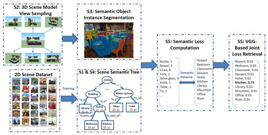
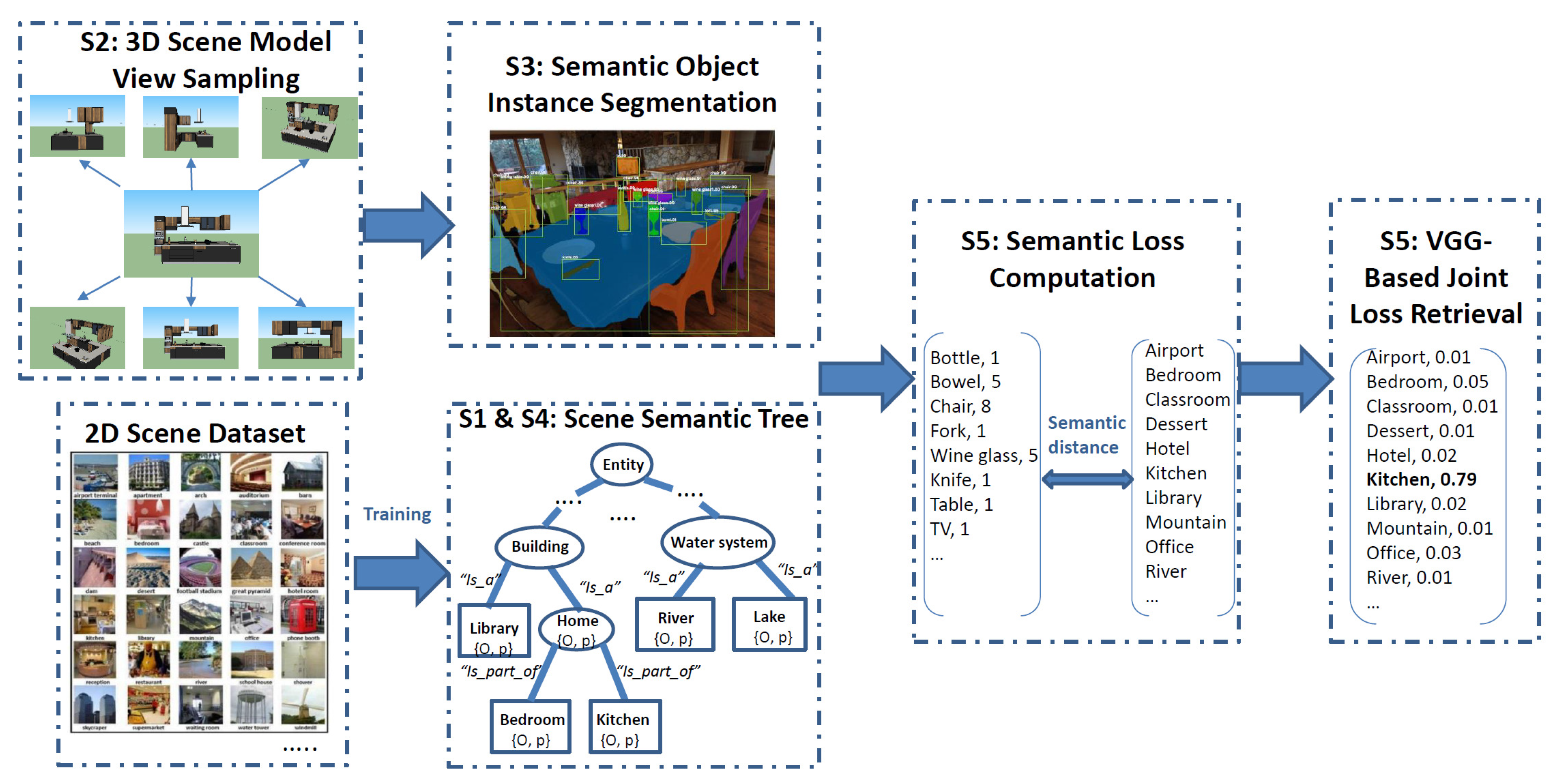
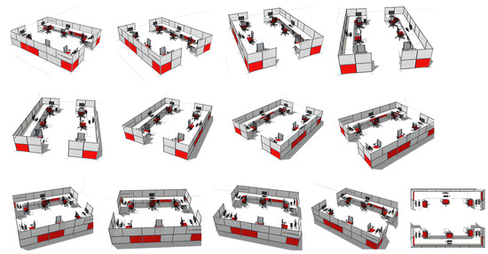
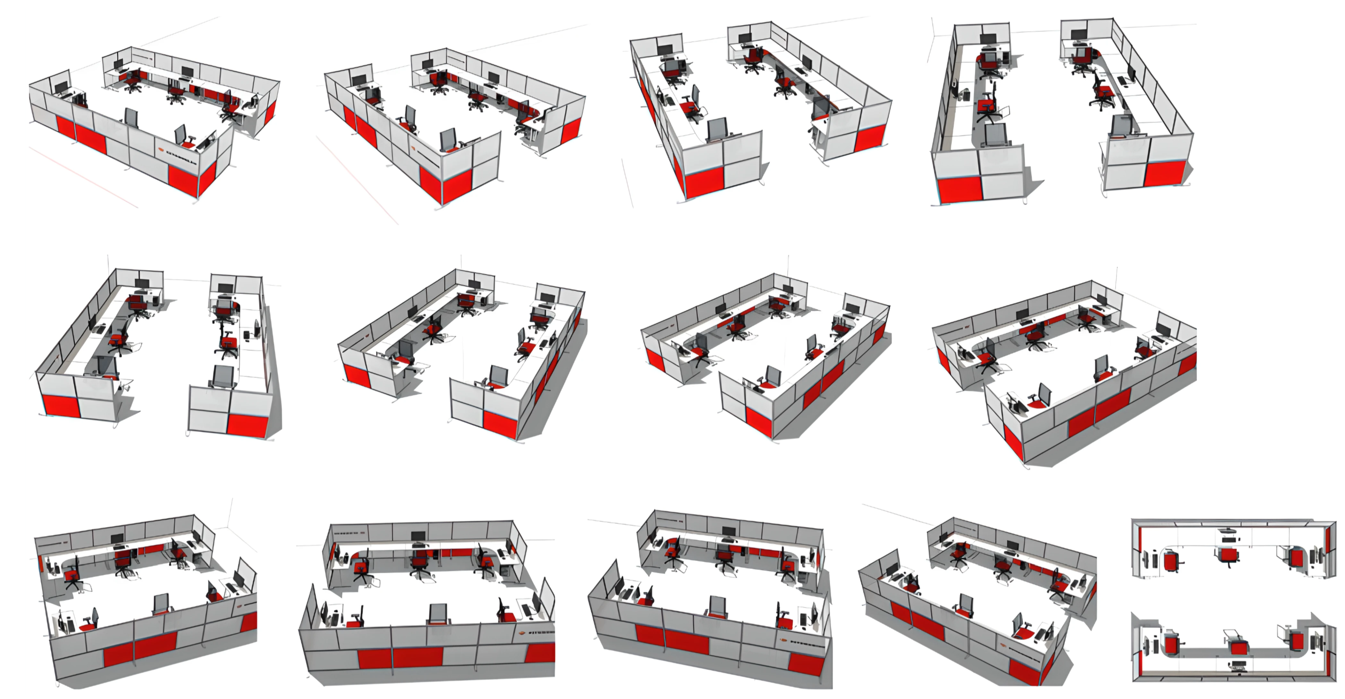
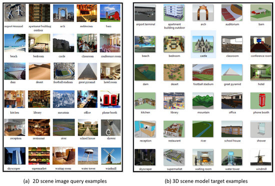
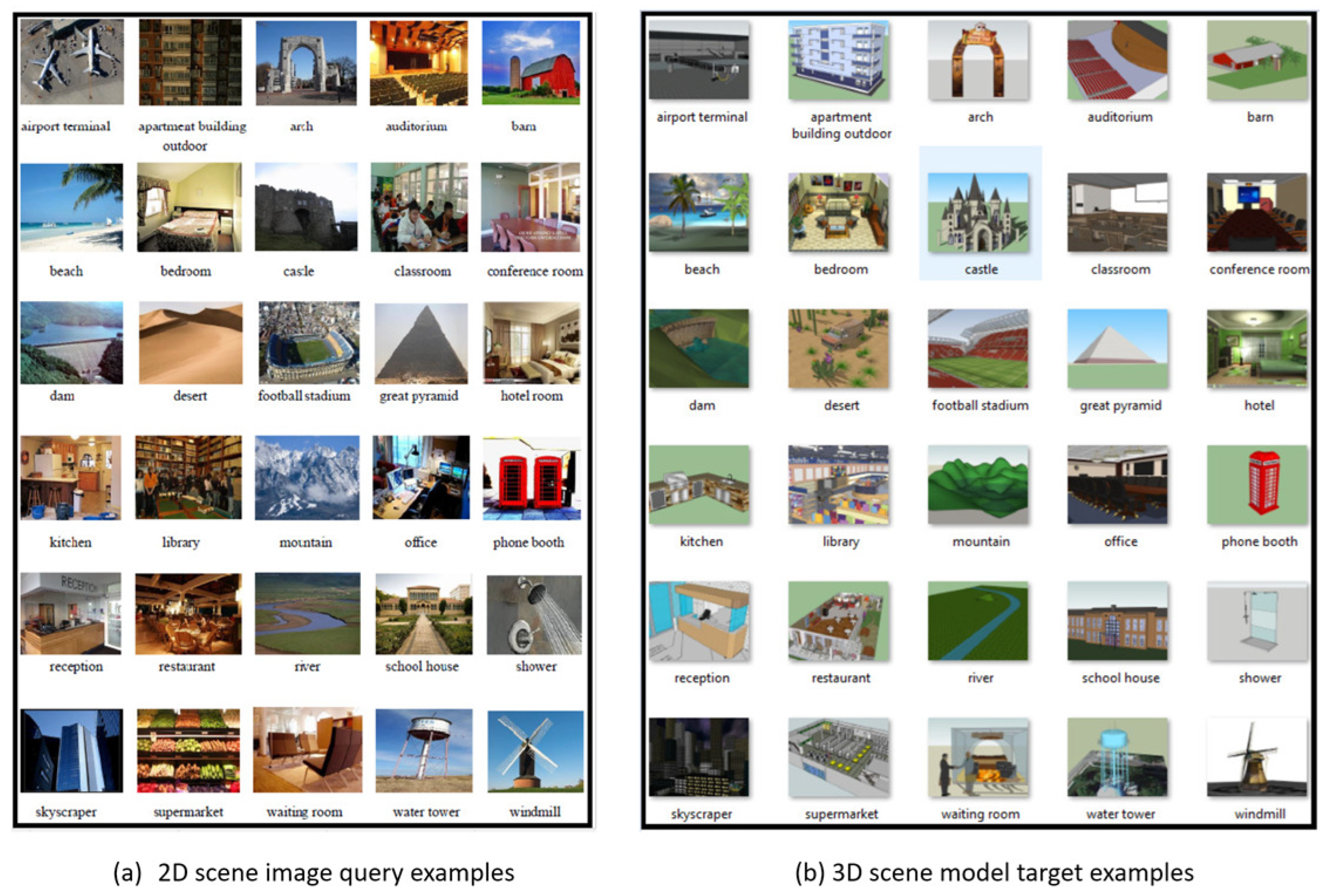
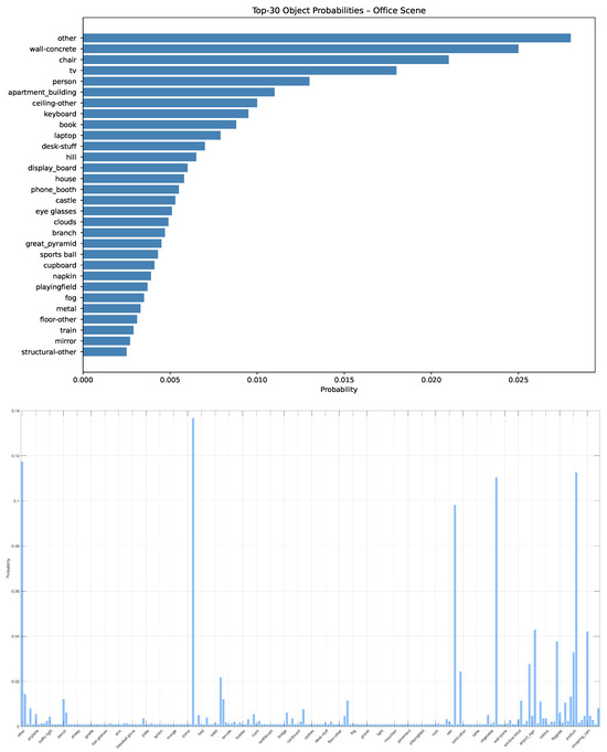
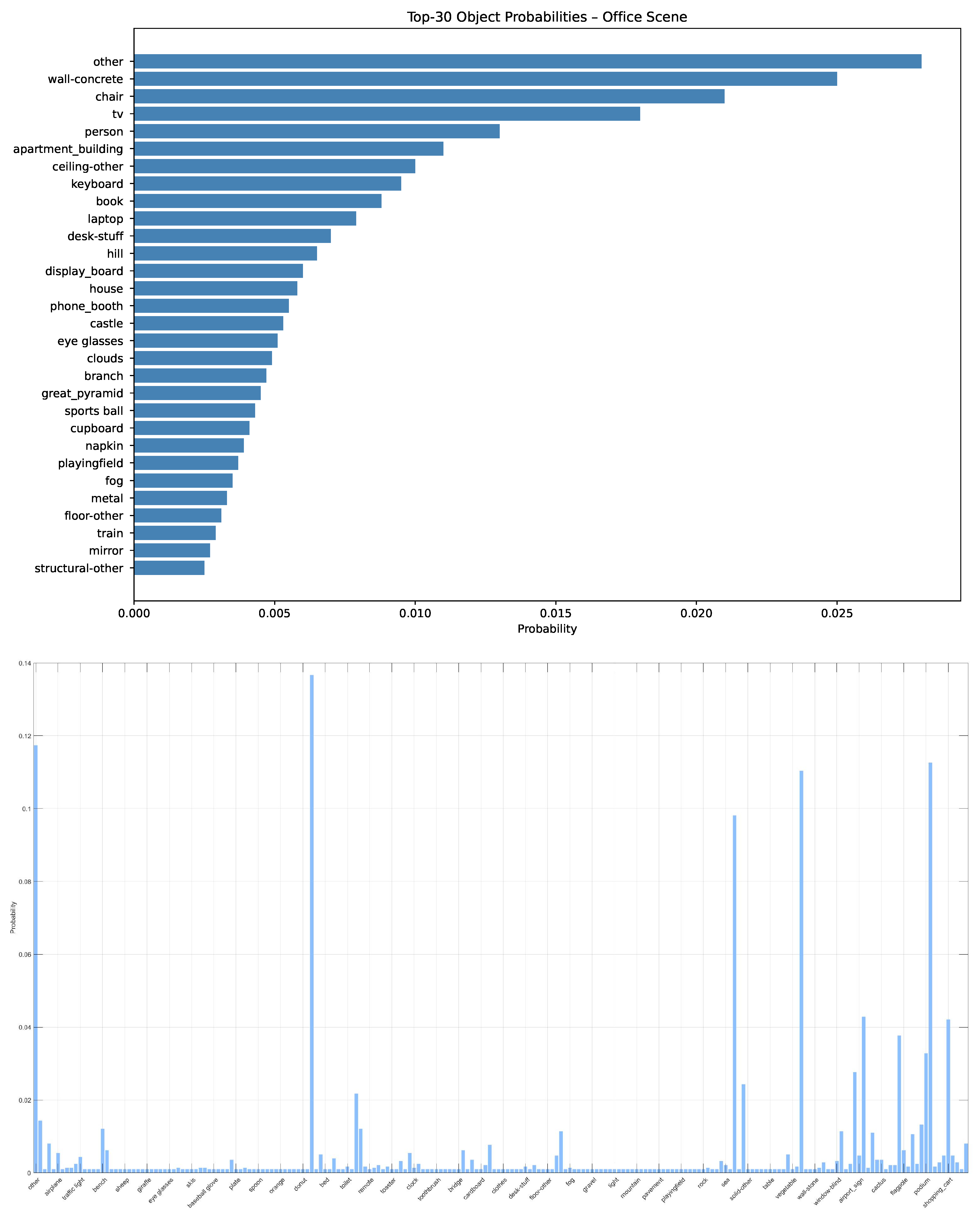
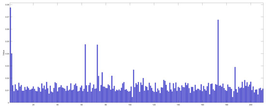
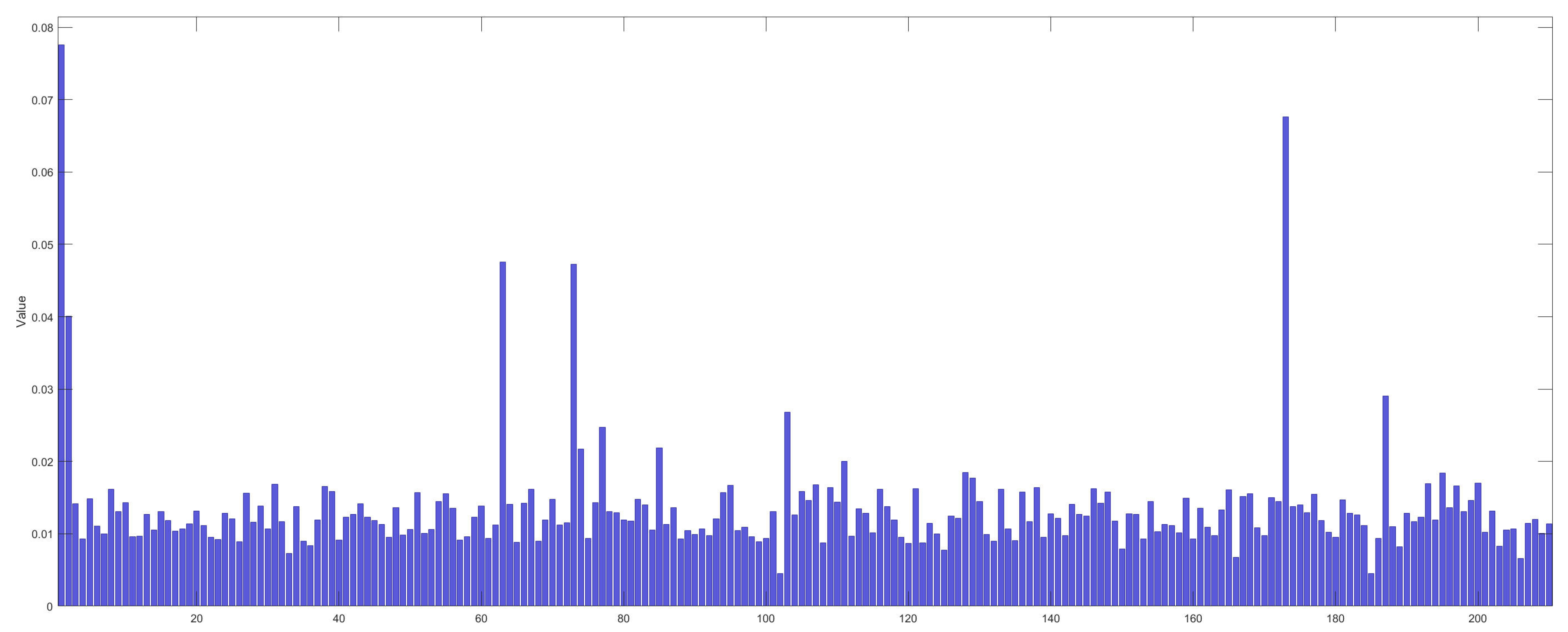
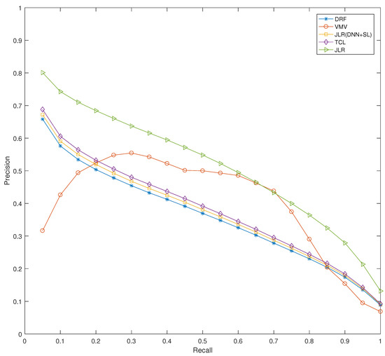
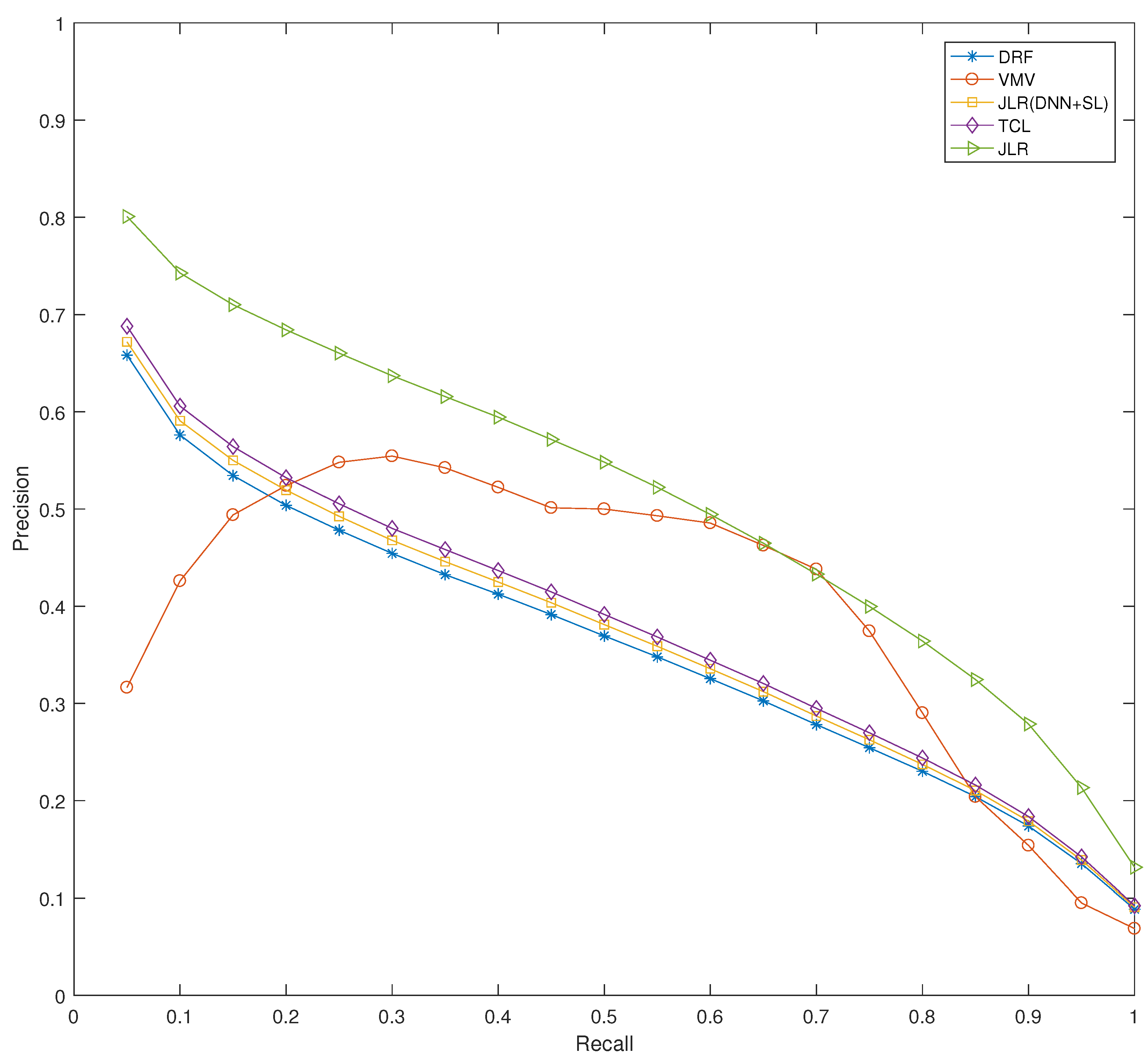
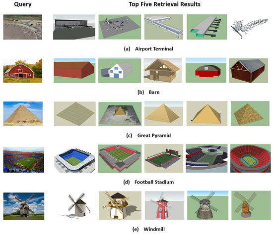
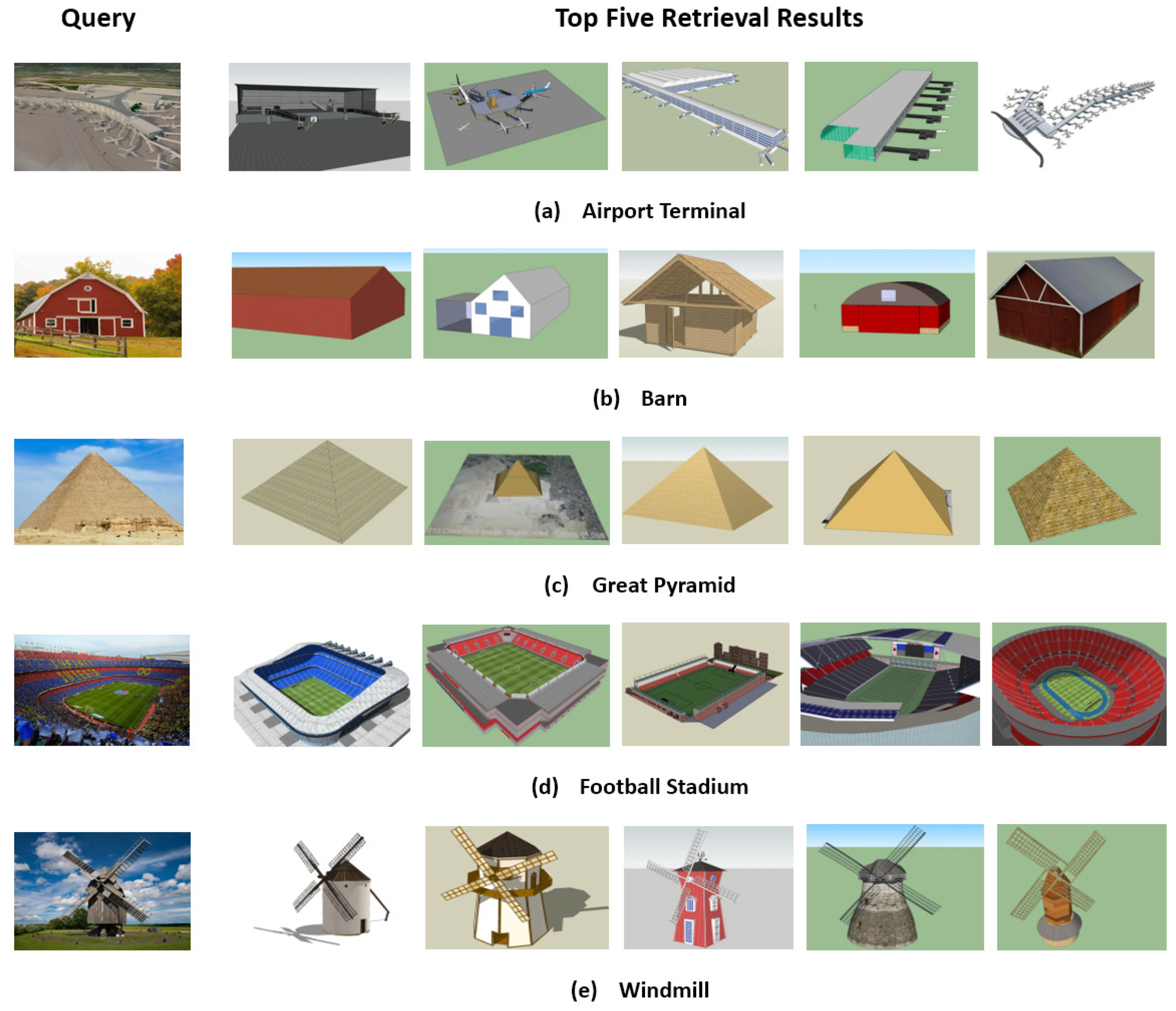

Disclaimer/Publisher’s Note: The statements, opinions and data contained in all publications are solely those of the individual author(s) and contributor(s) and not of MDPI and/or the editor(s). MDPI and/or the editor(s) disclaim responsibility for any injury to people or property resulting from any ideas, methods, instructions or products referred to in the content. |
© 2025 by the authors. Licensee MDPI, Basel, Switzerland. This article is an open access article distributed under the terms and conditions of the Creative Commons Attribution (CC BY) license (https://creativecommons.org/licenses/by/4.0/).