Abstract
To address the problems of the traditional Supply–Demand Optimization (SDO) algorithm in wireless sensor network (WSN) node deployment—such as blind search direction, weak global exploration capability, coarse boundary handling, and insufficient maintenance of population diversity—this paper proposes a Multi-Strategy Enhanced Supply–Demand Optimization algorithm (MESDO). The proposed MESDO is validated on the CEC2017 and CEC2022 benchmark test suites. The results demonstrate that MESDO achieves superior performance in unimodal, multimodal, hybrid, and composite function optimization: for unimodal functions, it enhances local exploitation precision via elite-guided search to quickly converge to optimal regions; for multimodal functions, the adaptive differential evolution operator effectively avoids local optima by expanding exploration scope; for hybrid and composite functions, the centroid-based opposition learning boundary control maintains stable population diversity, ensuring adaptability to complex solution spaces. These advantages enable MESDO to effectively avoid premature convergence. According to the Friedman test, MESDO ranks first on CEC2017 (d = 30), CEC2022 (d = 10), and CEC2022 (d = 20), with average rankings of 1.20, 1.67, and 1.33, respectively—significantly outperforming the second-ranked SDO (average rankings of 3.60, 3.25, and 3.83). Finally, MESDO is applied to WSN deployment optimization. Its average coverage rate (86.80%) exceeds that of SDO (84.41%) by 2.39 percentage points, while its minimum coverage (84.80%) is 21.21 percentage points higher than that of AOO (69.96%). Moreover, its standard deviation (8.1308 × 10⁻³) is the lowest among all compared algorithms. The convergence curve reveals that MESDO achieves 82% coverage within 50 iterations, which is significantly faster than SDO (80 iterations) and IWOA (100 iterations). The node deployment distribution further shows that the generated nodes are uniformly distributed without coverage blind spots. In summary, MESDO demonstrates superior optimization accuracy, convergence speed, and stability in both function optimization and WSN deployment, providing a reliable and efficient approach for WSN deployment optimization.
Keywords:
supply demand optimization; wireless sensor network; global optimization; elite-guided search; boundary control MSC:
68T20; 68W25; 68Q25
1. Introduction
With the rapid development of the Internet of Things (IoT), smart cities, environmental monitoring, and industrial automation, wireless sensor networks (WSNs)—as the core infrastructure for data acquisition and transmission—are gaining increasing importance. A WSN consists of numerous sensor nodes equipped with sensing, communication, and computing capabilities. These nodes can perform real-time monitoring, data aggregation, and remote transmission of physical environmental parameters (e.g., temperature, humidity, illumination, vibration) within a target area, providing fundamental data support for various intelligent applications. For instance, in environmental monitoring, WSNs can be deployed in forests, oceans, or remote mountainous regions to enable long-term, unattended observation of ecological changes [1,2]; in smart city construction, WSNs can be utilized for traffic flow monitoring, public safety alerts, and energy consumption management, thereby enhancing urban management efficiency [3]; in the industrial domain, WSNs can be embedded in production equipment and workshop environments to realize equipment condition monitoring and process optimization, driving the transformation toward Industry 4.0 [4,5].
As application demands continue to grow, the scale and coverage of WSN deployments have expanded rapidly, while performance requirements have become increasingly stringent. Sensor nodes are typically powered by batteries and often deployed in complex or harsh environments (e.g., outdoors, underground, or high-temperature and high-pressure industrial settings), making node replacement and maintenance both difficult and costly. Consequently, energy efficiency, coverage completeness, and network connectivity have become critical indicators that must be carefully considered during deployment. Moreover, WSN requirements vary significantly across different application scenarios [6]. For example, precision agriculture monitoring requires sensor nodes to be evenly distributed across farmland to ensure comprehensive data collection on crop growth conditions, whereas industrial equipment monitoring demands sensor nodes to be deployed closer to target devices to guarantee the accuracy and real-time performance of monitoring data [7,8]. These diverse and high-demand application contexts present new challenges and opportunities for the efficient deployment of WSNs.
Despite the broad application prospects of wireless sensor networks (WSNs), their deployment process still faces numerous challenges. First, in terms of coverage performance, random or grid-based node deployment often leads to uneven distribution, resulting in redundant nodes in some regions and sensing blind spots in others, thereby compromising data integrity. Second, since sensor nodes have limited and non-replenishable energy, unreasonable deployment may cause certain nodes to deplete their power prematurely due to frequent data forwarding, thus shortening the overall network lifetime. Third, node deployment must ensure network connectivity while minimizing deployment cost—an overly dense deployment increases interference and overhead, whereas a sparse deployment may create communication islands. Finally, traditional static deployment schemes struggle to adapt to dynamic factors such as node mobility and environmental changes, which can lead to network performance degradation. Therefore, achieving a comprehensive optimization that balances coverage, energy consumption, connectivity, and dynamic adaptability under limited resources remains a critical issue to be addressed in WSN deployment [9,10].
To address the aforementioned challenges in WSN deployment, traditional deployment methods—such as random deployment, grid-based deployment, and greedy algorithms—are no longer sufficient to meet the performance requirements of complex scenarios. Random deployment relies entirely on probabilistic distribution and cannot guarantee adequate coverage or network connectivity. Grid deployment, although capable of achieving uniform distribution, lacks flexibility and is difficult to apply to irregular regions or dynamic environments. Greedy algorithms, while capable of finding locally optimal solutions, tend to become trapped in local optima and fail to achieve global optimization of deployment performance. Against this backdrop, intelligent optimization algorithms have emerged as effective tools for WSN deployment optimization, owing to their strong global search capability, self-adaptive adjustment mechanisms, and multi-objective optimization ability [11,12].
Intelligent optimization algorithms are optimization methods inspired by natural phenomena, biological behaviors, or mathematical models. They can efficiently search for optimal solutions within complex solution spaces without relying on explicit mathematical formulations of the problem, thereby exhibiting strong generality and robustness [13]. When applied to WSN deployment optimization, intelligent optimization algorithms treat the sensor node coordinates as optimization variables, transforming objectives such as maximizing coverage, minimizing energy consumption, and maximizing network connectivity into optimization objective functions. Through iterative search processes, these algorithms identify deployment schemes that satisfy multiple objectives simultaneously [14]. For example, intelligent optimization algorithms can optimize the spatial distribution of sensor nodes to reduce coverage blind spots and node redundancy, balance energy consumption among nodes, and maintain network connectivity. Consequently, under limited node quantity and energy constraints, they can achieve global optimization of WSN deployment performance [12].
Swarm intelligence algorithms represent an important branch of intelligent optimization algorithms, inspired by the collective behaviors observed in biological populations. For instance, the Particle Swarm Optimization (PSO) algorithm [15] simulates the flight and foraging behavior of bird flocks, where each particle represents a candidate solution. The particles update their velocity and position through interaction with others, thereby searching for the optimal solution. The Ant Colony Optimization (ACO) algorithm [16] mimics the cooperative foraging behavior of ants, in which pheromone accumulation and evaporation guide the search toward optimal paths. The Grey Wolf Optimizer (GWO) [17] simulates the social hierarchy and hunting mechanism of grey wolves, where the α, β, and δ wolves guide the pack to encircle and attack the prey (optimal solution). The Whale Optimization Algorithm (WOA) [18] s inspired by the bubble-net hunting strategy of humpback whales, employing three mechanisms—encircling prey, spiral updating, and random search—to perform optimization. In recent years, numerous novel swarm intelligence algorithms have been developed. Examples include the Snake Optimizer (SO) [19], inspired by snakes’ foraging and reproductive behaviors; the Sparrow Search Algorithm (SSA) [20], based on the foraging and anti-predation behaviors of sparrows; and the Secretary Bird Optimization Algorithm (SBOA) [21], derived from the predatory behaviors of secretary birds. Similarly, the Grasshopper Optimization Algorithm (GOA) [22] models the social and swarming behaviors of grasshoppers, while the Remora Optimization Algorithm (ROA) [23] is inspired by the symbiotic relationship between remoras and their hosts during foraging. The Philoponella Prominens Optimizer (PPO) [24] simulates the unique mating, escape, and cannibalistic behaviors of Philoponella prominens. The Black Widow Optimization Algorithm (BWO) [25] draws inspiration from the distinctive reproductive behavior of black widow spiders, and the Dung Beetle Optimizer (DBO) [26] s modeled after dung beetles’ rolling, dancing, foraging, stealing, and reproductive behaviors. More recently, a physics-inspired approach known as the Kirchhoff’s Law Algorithm (KLA) [27] has been proposed, leveraging principles from circuit theory—particularly Kirchhoff’s Current Law (KCL)—to guide the optimization process.
For WSN deployment problems under different environmental conditions, researchers have proposed a variety of dynamic intelligent algorithm-based deployment strategies. For example, Yuan Yuting et al. proposed an Adaptive Hybrid Differential Grey Wolf Optimization (AHDGWO) algorithm to address issues such as large coverage blind spots and uneven node distribution in traditional WSN deployments, thereby improving two-dimensional coverage performance [28]. Xinyi Chen et al. introduced a hybrid Butterfly–Beluga Whale Optimization (NHBBWO) algorithm incorporating a dynamic secondary parameter adaptation strategy to enhance WSN coverage optimization [29]. Yong Zhang et al. developed an Adaptive Learning Fruit Fly Optimization Algorithm (FOA) to optimize node coverage and energy balance in both two-dimensional and complex three-dimensional environments [30]. Zhang Zhaohui et al. proposed a novel Semi-Fixed Clustering Algorithm (SFC-QL-IACO) aimed at maintaining energy balance within WSNs [31]. Xiaoyang Liu et al. designed a Hybrid Improved Compressed Particle Swarm Optimization (HICPSO) algorithm composed of a linearly decreasing inertia weight, compressed velocity vector, Gaussian-based population variation, and an optimal boundary selection mechanism for WSN node optimization [32]. Jiaming Wang et al. proposed an Improved Coverage Optimization Algorithm (ATSSA) based on an enhanced Salp Swarm Algorithm, aiming to improve network coverage while reducing node movement energy consumption during redeployment [33]. Although intelligent algorithms have achieved remarkable progress in WSN deployment optimization, an analysis of existing studies reveals that current methods still exhibit several limitations, which constrain their effectiveness in complex deployment scenarios.
The Supply–Demand Optimization (SDO) algorithm [34], inspired by the economic theory of supply–demand equilibrium, simulates the periodic fluctuation and balancing process of commodity prices and quantities to perform intelligent optimization. SDO is characterized by fast convergence and conceptual simplicity; however, it also suffers from several inherent limitations. Specifically, its equilibrium price selection relies on random probabilities or the population mean, without leveraging historical high-quality solutions, resulting in blind search directions and a tendency to fall into local optima in later iterations [35]. Furthermore, the algorithm updates solutions linearly via the supply–demand function, lacking a comprehensive global exploration mechanism. As equilibrium points are computed solely based on the population mean and no dynamic population updating strategy is adopted, population diversity rapidly diminishes, leading to a high risk of premature convergence. In addition, the boundary-handling mechanism of SDO simply resets out-of-bounds solutions randomly, discarding valuable positional information and ignoring the population distribution, thereby causing low information utilization efficiency [36,37].
To overcome the limitations of existing intelligent algorithms in WSN deployment—namely the imbalance between global exploration and local exploitation, insufficient population diversity, inefficient boundary control, and poor dynamic adaptability—this study proposes a Multi-Strategy Enhanced Supply–Demand Optimization (MESDO) algorithm for global optimization and node deployment in WSNs. The MESDO algorithm integrates three core enhancement strategies to improve its search efficiency, robustness, and adaptability. First, an elite-guided search strategy is designed to dynamically construct an elite pool and use elite solutions to guide the selection of equilibrium prices, thereby maintaining a balance between search precision and population diversity. Second, an adaptive differential evolution operator is introduced to dynamically adjust the mutation factor and incorporate guidance from the global best solution, enhancing the algorithm’s global exploration capability. Finally, a centroid-based opposition learning boundary control strategy is proposed, which corrects out-of-bounds solutions with reference to the population centroid—preserving effective positional information and avoiding invalid searches.
To further clarify the differences between this study and existing achievements and highlight the innovations, Table 1 summarizes the core features of representative intelligent optimization algorithms used for Wireless Sensor Network (WSN) deployment optimization. The comparison is conducted across key dimensions such as strategy design, search capability, and intuitively demonstrates the advantages of this research.

Table 1.
Comparison of proposed MESDO with existing algorithms for WSN deployment.
The main contributions of this work are as follows:
- (1)
- A multi-strategy enhanced supply-demand optimization algorithm (MESDO) is proposed, based on an elite-guided search strategy, an adaptive differential evolution operator strategy, and a centroid-based opposition learning boundary control strategy;
- (2)
- The overall performance of MESDO is comprehensively evaluated on the CEC2017 and CEC2022 benchmark suites;
- (3)
- A mathematical model for WSN deployment is constructed, and MESDO is applied to solve it, with comparative analysis against other algorithms demonstrating MESDO’s effectiveness in WSN scenarios.
The remaining chapters of this paper are organized as follows: Section 2 elaborates on the principles of the traditional supply-demand optimization (SDO) algorithm and introduces the design logic and mathematical models of the three core enhancement strategies of MESDO; Section 3 provides a comprehensive validation of MESDO through numerical experiments on the CEC2017 and CEC2022 benchmark suites; Section 4 constructs a mathematical model for WSN deployment and compares the deployment performance of MESDO with other algorithms through simulation experiments, evaluating its advantages in practical applications from the perspectives of coverage, convergence curves, and node distribution; Section 5 concludes the study, analyzes its limitations, and discusses future research directions.
2. Supply Demand Optimization (SDO) and the Proposed Methodology
2.1. Supply Demand Optimization (SDO)
The supply-demand optimization (SDO) algorithm was first proposed by Zhao et al. in 2020, inspired by economic theory. In this theory, the price and quantity of a commodity undergo cyclical fluctuations and gradually stabilize at their respective equilibrium points. In a market economy, the supply-demand mechanism forms the core theory for price determination. Specifically, the supply relationship of producers determines the quantity of a commodity in the next period , which depends on the current commodity price , and can be expressed as , where represents a linear supply function. Therefore, when the current price of a commodity rises in the market, the supply quantity in the next period will also increase, indicating that is a monotonically increasing function. In addition, consumers’ demand relationship determines the price of the commodity in the next period, which depends on the quantity of the commodity in the same period and can be expressed as , where represents a linear demand function. It can be seen from this that when the quantity of the commodity increases, its price in the market will decrease, so is a decreasing function. In the process of fluctuation, these two functions will intersect at the equilibrium point . Among them, and represent the equilibrium price and equilibrium quantity of the commodity, respectively. Therefore, the supply function and the demand function can be expressed as [34,36]:
in the equation, represents time, and and are the linear coefficients.
To describe the changes in commodity prices and quantities, two matrices are introduced. When the demand function is less than the supply function , the fluctuation amplitude will be small. After a period of time, the quantity and price curves of commodities will stabilize over time and converge to the equilibrium point . At this time, it is in a stable mode. However, when the supply function is less than the demand function , the fluctuation amplitude will increase. After a period of time, the quantity and price curves of commodities will move away from the equilibrium point over time. The mathematical expression of this algorithm is constructed as follows: the market quantity is represented by , each market contains different commodities, and each type of commodity has specific quantities and prices. As variables, each candidate solution and possible candidate solution are, respectively, composed of commodity prices and commodity quantities. As shown in Equation (2), there are stable mode and unstable mode. In the stable mode, the demand function is less than the supply function , as shown in [34,36].
where and represent candidate solutions and potential candidate solutions, respectively, and are associated through a fitness function. The fitness function can be arranged into an array as shown in Equation (3) to represent the fitness values of these two vectors.
The characteristic description of the equilibrium quantity vector is shown in Equation (4), where the transpose of the array is denoted by .
In the equations, denotes the roulette wheel selection method. According to Equation (6), the algorithm assumes that, based on the probabilities corresponding to the equilibrium price vector in the price array, there is a 50% chance of selecting either the average of the price vectors or the current price vector:
where is a random number in the interval [0, 1].
Subsequently, as shown in Equations (7) and (8), in each market, the supply and demand functions are updated based on the equilibrium price vector and equilibrium quantity vector [34,36]:
where and represent the price vector and quantity vector of the -th commodity at time , and are the supply and demand weights, respectively. By substituting Equation (7) into Equation (8), the demand equation can be rewritten as:
From Equation (9), it can be seen that the update of the commodity price vector is based on the current price vector while considering the equilibrium price vector. Therefore, by adjusting the values of and , different commodity price vectors can be generated, which, as shown in Equation (10), enable the exploration and exploitation processes [34,36].
where denotes the maximum number of iterations, and is a random number in the interval [0, 1].
2.2. Proposed Multi-Strategy Enhanced Supply Demand Optimization (MESDO)
2.2.1. Elite-Guided Search Strategy
In the standard SDO algorithm, the selection of the price equilibrium point during iterations relies on random probability or the population mean, lacking utilization of historical high-quality solutions. This results in a blind search direction, particularly in the later stages of iteration, making the algorithm prone to local optima or slower convergence. To address this, the MESDO algorithm introduces an elite-guided search strategy, which dynamically constructs an elite pool and uses elite solutions to guide the selection of price equilibrium points, achieving a balance between search accuracy and population diversity.
The elite-guided search strategy focuses on leveraging the guiding value of historical high-quality solutions. Its implementation logic is as follows: First, in each iteration, the price solutions of all markets (i.e., the current better solutions in each market) are extracted as elite candidate solutions, and their corresponding fitness values are recorded simultaneously. Next, the candidate solutions are sorted in ascending order based on their fitness values, and the top solutions (with defaulted to no more than 5 and not exceeding the population size to avoid an unreasonably large elite pool, this parameter was determined through parameter sensitivity analysis.) are selected to form a dynamic elite pool. Finally, the guiding elite is selected based on random probability—with a 10% chance, the mean of all solutions in the elite pool is chosen (to ensure exploration of globally high-quality regions), and with a 90% chance, a single solution is randomly selected from the elite pool (to ensure deep exploitation of locally high-quality regions). The selected guiding elite is defined as .
During the price equilibrium point selection stage, to fully leverage the guidance of elite solutions, the MESDO algorithm adjusts the original SDO logic: as showed in Figure 1, when the random probability is greater than 0.3, is directly used as the price equilibrium point , guiding the generation of new solutions toward the high-quality region where the elite resides; when the random probability is no greater than 0.3, the original SDO selection logic is retained (i.e., 50% chance to select the population price mean, 50% chance to select a single price solution based on fitness probability), avoiding over-reliance on elite solutions that could reduce population diversity.
where represents the mth elite solution in the elite pool, is the fixed size of the elite pool, and denotes a randomly selected individual from the elite pool. This formula, by averaging the elite solutions, reduces the interference from potential local optima of a single elite solution and ensures stable guidance toward globally high-quality regions.
Figure 1.
Elite-guided search strategy diagram.
2.2.2. Adaptive Differential Evolution Operator Strategy
The standard SDO algorithm updates quantity and price solutions solely through the supply and demand functions, lacking a global exploration mechanism for the solution space. In complex high-dimensional optimization problems, this can lead to overly strong local search, causing the algorithm to become trapped in local optima and making it difficult to escape inefficient solution regions. To address this, the MESDO algorithm introduces an adaptive differential evolution operator strategy, as illustrated in Figure 2, which dynamically adjusts the mutation factor and incorporates guidance from the global best solution to enhance the algorithm’s global exploration capability and convergence efficiency.
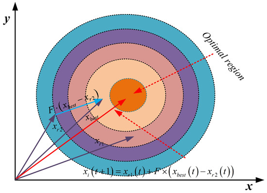
Figure 2.
Schematic diagram of adaptive differential evolution strategy.
and denote two distinct individuals randomly selected from the population , represents the global best solution, and is the mutation factor, which is calculated as follows:
The parameter is bounded by and Its value is decremented linearly across the total number of generations, . This progressive scaling allows the search behavior to evolve from widespread exploration during initial phases to intensified exploitation near the conclusion.
This strategy introduces to guide the mutation direction, allowing the mutated solutions to move closer to globally high-quality regions, thereby avoiding the blind randomness inherent in the traditional DE mutation operator.
2.2.3. Centroid-Based Opposition Learning Boundary Control Strategy
In the standard SDO algorithm, out-of-bounds solutions are handled by randomly resetting the offending dimensions within the feasible domain. This approach completely discards the original positional information of the out-of-bounds solutions and does not utilize population distribution characteristics, which can result in corrected solutions being far from high-quality regions and increase search randomness—leading to population disorder in the early iterations and potentially disrupting high-quality search trends in later stages, thereby reducing optimization accuracy.
To address this, MESDO proposes a centroid-based opposition learning boundary control strategy. The core idea is to use the current population centroid (mean) as a reference to perform opposition-based correction on out-of-bounds solutions. First, the centroid vector is calculated as the mean of all solution dimensions in the population; if the upper and lower bounds are scalars, they are expanded to match the population size across all dimensions. Next, all out-of-bounds dimensions (below the lower bound or above the upper bound) are identified, and each out-of-bounds dimension is corrected using the formula centroid value minus the original out-of-bounds value,” thereby preserving the positional relationship between the out-of-bounds solution and the centroid. Finally, the solution is truncated by the upper and lower bounds to ensure feasibility and prevent secondary boundary violations.
As shown in Figure 3, by adjusting the positions of individuals exceeding the boundaries and mapping them back into the valid search space, invalid searches are avoided and convergence speed is improved. This process is described by Equation (14).
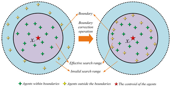
Figure 3.
Schematic diagram of centroid-based opposition learning boundary control strategy.
Based on the above discussion, the pseudocode for MESDO is presented in Algorithm 1.
| Algorithm 1. Pseudo-Code of MESDO. |
| 1: Initialize the SDO parameters (population , ), Max iterations . 2: Initialize the vectors and calculate their fitness value . 3: while do 4: Calculate the weights and . 5: Calculate 6: for each market 7: Determine the equilibriu m quantity by Equation (4). 8: Determine the equilibriu m price by Equation (5). 9: Update the commodity quantity vector by Equation (7). 10: Update the commodity quantity vector by Equation (8). 11: Centroid-based opposition learning boundary control strategy by Equation (14). 12: Calculate their fitness values and . 13: Apply adaptive differential evolution strategy to update solutions using Equations (12) and (13). 14: if do 15: replace by . 16: end if 17: end for 18: Update the best solution found so far . 19: end while 20: Return . |
3. Numerical Experiments
3.1. Competitor Algorithms and Parameters Setting
In this section, the performance of the proposed MESDO algorithm is rigorously evaluated using two highly competitive numerical optimization benchmark suites: CEC2017 [38] and CEC2022 [39]. For comparison, multiple state-of-the-art algorithms are included, such as Velocity Pausing Particle Swarm Optimization (VPPSO) [40], MadDE [41], Improved multi-strategy adaptive Grey Wolf Optimization (IAGWO) [42], Improved Whale Optimization Algorithm (IWOA) [43], Status-based optimization Algorithm (SBO) [44], Animated Oat Optimization (AOO) [45], Holistic swarm optimization (HSO) [46], and Supply demand optimization (SDO) [34]. Configuration details for all benchmarked algorithms are presented in Table 2.
Table 2.
Compare algorithm parameter settings.
3.2. Qualitative Analysis of MESDO
3.2.1. Analysis of the Population Diversity
The efficacy of population-based optimizers is heavily influenced by a fundamental property: population diversity, which reflects the distribution and dissimilarity of individual solutions [47]. Maintaining robust diversity is essential for preventing premature convergence and ensuring thorough exploration of the solution space, thereby underpinning search robustness. A quantitative evaluation of diversity within the MESDO framework, based on Equation (15) [48], is presented hereafter.
A measure designated as characterizes the variety within a population of size . This metric is based on , a quantity expressing the collective spread of all agents in relation to their central point at time . The calculation for is provided in Equation (16), and it aggregates the coordinates for every member in each dimension .
Figure 4 illustrates the evolution curves of population diversity for the MESDO and the original SDO algorithms on 10 representative functions (F1, F5, F10, F12, F15, F17, F18, F22, F27, F30) from the CEC2017 benchmark suite (dimension ). The diversity metric is calculated using Equation (15), measuring the dispersion of the population relative to the centroid .
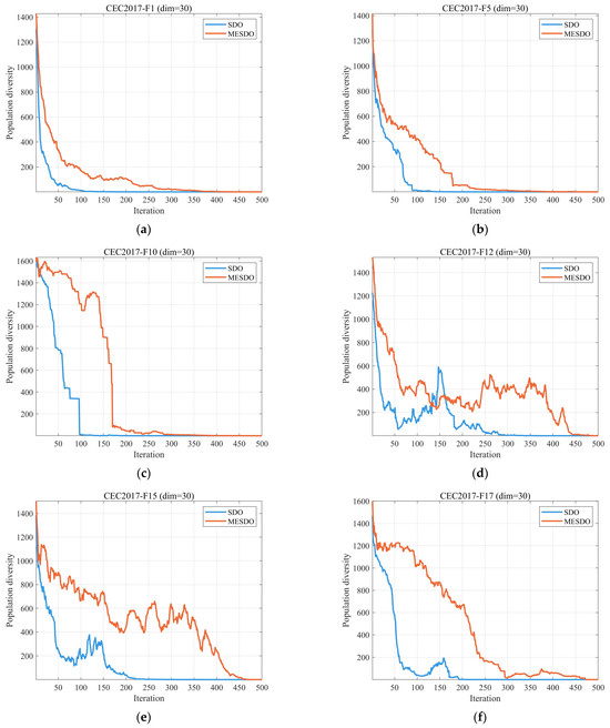
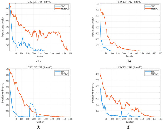
Figure 4.
A comparative assessment of population distribution for the MESDO and SDO techniques.
From the overall evolutionary trend, MESDO maintains significantly higher population diversity than SDO throughout the entire iteration process, with a smoother decline as iterations progress. This phenomenon results from the synergistic effects of MESDO’s three core strategies: the elite-guided search strategy, via a dynamic elite pool and probabilistic guidance mechanism, prevents the population from prematurely converging to local optima; the adaptive differential evolution operator strategy, through mutation guided by the global best solution, continuously injects new diversity into the population; and the centroid-based opposition learning boundary control strategy preserves the positional relationship between out-of-bounds solutions and the population centroid, preventing loss of effective diversity.
Examining different types of functions in detail, for the unimodal function F1, MESDO’s diversity curve consistently stays above that of SDO (with an average difference exceeding 300), demonstrating that it maintains global exploration capability even during local exploitation. For the multimodal functions F5, F10, and F12, MESDO’s higher diversity effectively avoids the premature convergence commonly seen in SDO, especially in later iterations (after 300 generations), where SDO’s diversity stabilizes while MESDO maintains diversity above 400, supporting continued exploration of new high-quality solution regions. For the hybrid and composite functions F15, F18, F22, F27, and F30, MESDO’s diversity advantage becomes even more pronounced; for instance, at 500 iterations on F30, MESDO’s s approximately twice that of SDO, fully demonstrating its ability to balance exploration and exploitation in complex solution spaces.
Furthermore, the sudden jump in population diversity observed in subfigures (d) (CEC2017-F12 function) and (i) (CEC2017-F27 function) of Figure 4 is essentially an adaptive adjustment of the algorithm in response to the complex characteristics of the functions, rather than a convergence anomaly. This is because F12 and F27 are multimodal functions with a large number of local optima in the solution space, and these local optimal regions are widely distributed. The sudden increase in diversity around the 300th generation is primarily due to the active exploration of the adaptive differential evolution operator: at this mid-iteration stage, the mutation factor F remains around 0.4 (according to Equation (13), F decreases linearly with iterations), and the algorithm triggers a large-scale mutation operation guided by the global optimal solution. This operation breaks the previously trapped local optimal convergence state of the population, allowing some individuals to escape the current local optimal region and explore new high-potential solution spaces, directly manifesting as a sudden increase in population diversity. This jump is a key mechanism for the algorithm to avoid premature convergence. The subsequent diversity curve continues to decline steadily, proving that the algorithm does not enter an unstable state.
In summary, the results in Figure 4 confirm that MESDO, through its strategic improvements, significantly enhances the maintenance of population diversity, providing a strong foundation for overcoming local optima and improving optimization accuracy in subsequent tasks.
3.2.2. Exploration and Exploitation Dynamics
Optimization algorithms operate through two complementary search paradigms: exploration, which entails a widespread investigation of the solution space to identify regions of potential, and exploitation, which involves a concentrated effort to hone high-quality solutions [49,50]. A bias towards the former can lead to inefficient, unproductive search; a dominance of the latter often traps the algorithm in local optima. Consequently, the strategic equilibrium between them is a decisive factor for success. The subsequent analysis evaluates this balance within the MESDO framework, applying the metrics defined in Equations (17) and (18) [48,50].
The normalized diversity at iteration is defined as the ratio of the current diversity, —computed from Equation (19)—to the maximum diversity value, , observed across all iterations.
Figure 5 presents the dynamic evolution of exploration and exploitation for the MESDO algorithm on representative functions (F1, F5, F16, F2, F26, F30) from the CEC2017 benchmark suite (dimension ). The exploration rate and exploitation rate are calculated using Equations (17) and (18), respectively, measured by the ratio of the diversity metric (defined in Equation (19), reflecting the dispersion of each dimension in the population relative to the median) to the maximum diversity .
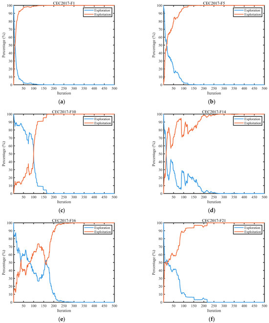
Figure 5.
Examination of the global search and local refinement capabilities in MESDO.
From the evolution curves, it can be observed that MESDO achieves an adaptive dynamic balance between exploration and exploitation throughout the entire iteration process. This core regulatory mechanism stems from the synergistic effects of the three strategies: the adaptive differential evolution (DE) operator strategy maintains a high exploration rate (60–90%) during the early iterations (1–150 generations) through the linear decrease in the mutation factor FFF (as shown in Equation (13), where decreases from to ), supporting efficient global exploration of the solution space. For example, in function F1, the exploration rate exceeds 85% in the early iterations, effectively covering multimodal regions.
The elite-guided search strategy, during the middle iterations (150–300 generations), gradually increases the exploitation rate (from 30% to 60%) by guiding the selection of price equilibrium points with a 90% probability of choosing a single solution from the elite pool, enabling deep exploitation of high-quality solution regions. Taking function F5 as an example, the exploitation rate steadily rises during this stage, while the exploration rate remains above 30%, preventing premature convergence to local optima.
The centroid-based opposition learning boundary control strategy, in the later iterations (300–500 generations), preserves basic population diversity by correcting out-of-bounds solutions, maintaining the exploration rate at 20–40% and the exploitation rate at 60–80%. This ensures precise convergence toward the global optimum while preventing excessive loss of population diversity.
3.2.3. Performance Impact of the Proposed Strategy
A methodical ablation framework was established to dissect the individual efficacy and synergistic interactions of the three core innovations: the Elite-guided search strategy (S1), Adaptive differential evolution operator strategy (S2), and Centroid-based opposition learning boundary control strategy (S3). Utilizing the CEC2017 benchmark (d = 30), we evaluated five algorithmic variants: the standard SDO, three partial implementations (SDO-S1, SDO-S2, SDO-S3), and the complete MESDO. This design allows for clear efficacy attribution, with the comparative results detailed in Figure 6 and Figure 7.
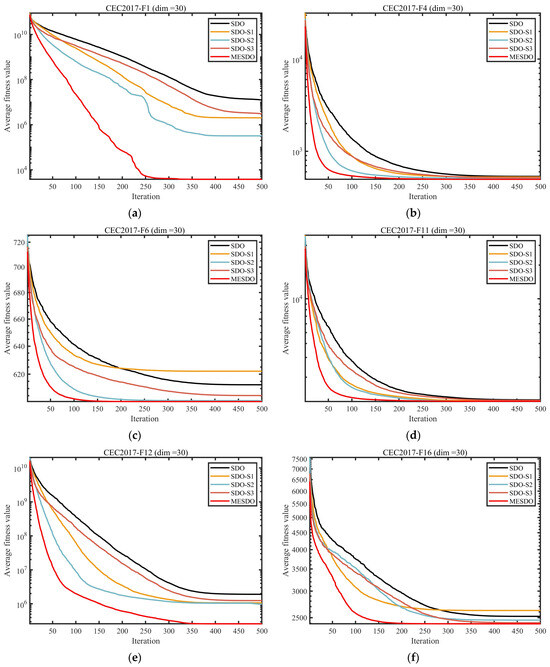
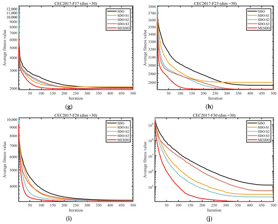
Figure 6.
Efficacy analysis of different strategic enhancements.
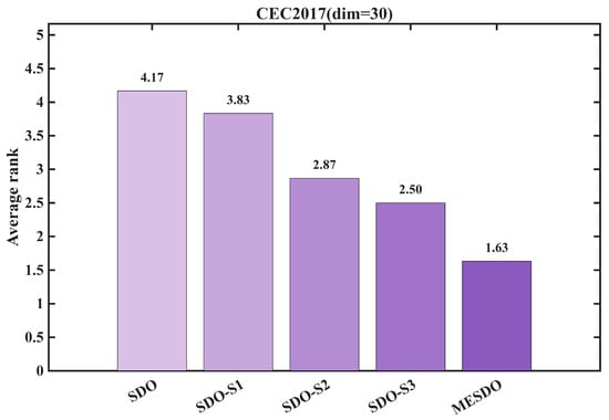
Figure 7.
Comparative performance ranking of SDO variants with different enhancements.
The convergence curves in Figure 6 indicate that while each of the three strategies enhances performance differently, their combination produces a significant synergistic effect. For unimodal functions, SDO-S1 (integrating S1) accelerates convergence by guiding the search direction with elite solutions, entering high-quality regions earlier than the original SDO. SDO-S2 (integrating S2), leveraging mutation operations guided by the global best solution, demonstrates stronger global exploration in the early iterations, quickly covering critical areas of the solution space. SDO-S3 (integrating S3), through boundary control, reduces ineffective searches, resulting in significantly more stable convergence in the later iterations compared with the original SDO, avoiding performance fluctuations caused by random resets of out-of-bounds solutions. The complete MESDO algorithm, benefiting from the synergy of the three strategies, shows a convergence curve with no noticeable oscillations and consistently outperforms all comparison algorithms, achieving optimization accuracy far superior to both the original SDO and single-strategy variants. This demonstrates the efficient coordination of “global exploration—local exploitation—stable convergence”.
For multimodal functions, SDO-S2 contributes most to escaping local optima, effectively mitigating the original SDO’s tendency to become trapped. MESDO further enhances this capability by combining S1’s precise localization of high-quality regions with S2’s global exploration, achieving better optimization accuracy than any single-strategy variant. In composite functions, SDO-S3’s boundary control plays a key role in maintaining population diversity, preventing the sharp decline in diversity observed in the original SDO within complex solution spaces. MESDO, through the synergy of S3 with S1 and S2, maintains stable performance improvements even in the later iterations, ultimately achieving superior optimization results compared with all other algorithms.
The average ranking results in Figure 7 further quantify the overall gains of each strategy. The original SDO ranks relatively low, whereas SDO-S1, SDO-S2, and SDO-S3 all show improved average rankings, indicating that each single strategy can enhance algorithm performance from different perspectives. Among them, SDO-S2 provides the most significant independent gain, with a greater improvement in average ranking than SDO-S1 and SDO-S3. The complete MESDO algorithm, however, achieves the best average ranking across all test functions, consistently placing first, demonstrating the advantage of the three strategies’ synergy. This ranking shows that the strategies do not simply superimpose their effects, but form an efficient cooperative mechanism: S1 addresses the blind search direction of the original SDO, providing precise guidance for S2’s global exploration and avoiding ineffective searches; S2 compensates for SDO’s insufficient global exploration, supporting S1’s local exploitation with a broader base of high-quality solutions and expanding coverage of high-quality regions; S3 ensures population diversity through boundary corrections, providing a stable population environment for the continuous action of S1 and S2, preventing performance stagnation due to diversity loss.
In summary, the combined analysis of Figure 6 and Figure 7 fully validates the effectiveness and synergistic value of MESDO’s core strategies. A single strategy can improve algorithm performance in terms of search direction, exploration capability, and convergence stability, whereas the synergy of all three strategies produces an optimization effect of “1 + 1 + 1 > 3.” This lays a solid strategic foundation for MESDO to achieve high optimization accuracy, fast convergence, and strong stability in complex optimization problems, and also provides a reference design idea for multi-strategy improvements in other optimization algorithms.
3.3. Performance Evaluation Using CEC2017 and CEC2022 Benchmark Problems
This section presents a comparative evaluation of MESDO with other benchmark algorithms using the CEC2017 and CEC2022 test suites. These benchmark sets comprise four categories of mathematical functions: unimodal, multimodal, hybrid, and composition functions. Multimodal functions, characterized by multiple local optima, are effective for testing an optimizer’s exploration capability. In contrast, unimodal functions—featuring a single global optimum—primarily gauge exploitation performance. Hybrid and composition functions further examine an algorithm’s capacity to escape local optima.
To ensure fairness and minimize random effects, all algorithms were configured with a population size of 30 and a maximum of 500 iterations. Each method was executed independently 30 times. The average (Ave) and standard deviation (Std) of the results are reported, with optimal values emphasized in bold. Experiments were performed on a Windows 11 platform with an AMD Ryzen 7 9700X 8-Core Processor (3.80 GHz), 48 GB RAM, and MATLAB 2024b. Convergence behavior and distribution characteristics of the algorithms are visually compared in Figure 8 and Figure 9 through convergence curves and box plots, respectively.
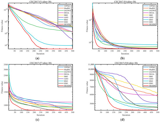
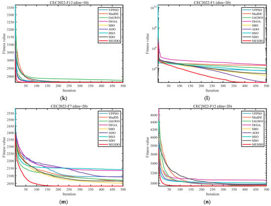
Figure 8.
Comparison of convergence speed of different algorithms on test set.
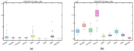
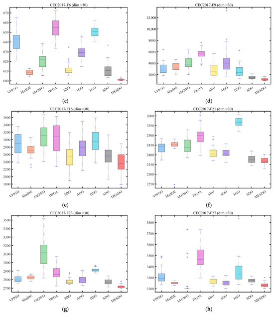
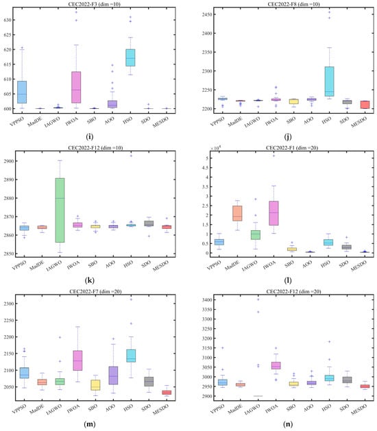
Figure 9.
Boxplot analysis for different algorithms on the test set.
Table 3, Table 4 and Table 5 (CEC2017, d = 30), 3 (CEC2022, d = 10), 4 (CEC2022, d = 20), and Figure 8 and Figure 9 comprehensively analyze the performance advantages of MESDO compared with eight benchmark algorithms, including VPPSO, MadDE, IAGWO, IWOA, SBO, AOO, HSO, and SDO, across different test scenarios, function types, and dimensional conditions.
Table 3.
Experimental findings on the CEC2017 benchmark suite (d = 30).
Table 4.
Experimental findings on the CEC2022 benchmark suite (d = 10).
Table 5.
Experimental findings on the CEC2022 benchmark suite (d = 20).
In the complex function scenario of the CEC2017 (d = 30) test set, unimodal functions (F1–F7) evaluate the algorithm’s local exploitation capability. For F1, a basic unimodal function, MESDO achieves an average fitness value (Ave = 2.0944 × 10³) far lower than the original SDO (1.1519 × 10⁷) and VPPSO (1.0818 × 10⁷), only 1/5500 and 1/5160 of their values, respectively, and also surpasses the next best performer HSO (7.8563 × 10³), achieving 1/3.75 of its value. Its standard deviation (Std = 1.8539 × 10³) is only 1/7450 of SDO (1.3814 × 10⁷), demonstrating highly precise convergence with minimal performance fluctuation across repeated runs. F3, a noisy unimodal function, sees MESDO achieve Ave = 6.2832 × 10³, reducing 75% relative to SDO (2.4989 × 10⁴) and 61% relative to SBO (1.6155 × 10⁴), with Std = 3.4882 × 10³, only 1/12.6 of IWOA (4.4143 × 10⁴), highlighting its robust local exploitation even under noise interference.
Multimodal functions (F8-F13) require overcoming local optima. For F9, a high-dimensional multimodal function, MESDO achieves Ave = 1.1916 × 10³, 23% lower than SDO (1.5538 × 10³) and 55% lower than HSO (2.6749 × 10³), with Std = 1.8556 × 10², only 1/5.1 of VPPSO (9.5445 × 10²), demonstrating the efficacy of the adaptive differential evolution operator in escaping local optima. For F12, a complex multimodal function, MESDO achieves Ave = 2.0569 × 10⁵, 91% lower than SDO (2.3800 × 10⁶) and 59% lower than HSO (5.0311 × 10⁵), with Std = 1.8228 × 10⁵ far below SDO (2.1727 × 10⁶), reflecting high global exploration precision in multimodal solution spaces.
For hybrid and composite functions (F14–F30), which integrate multiple solution space characteristics, F15, a hybrid function, shows MESDO achieving Ave = 6.3207 × 10³, 37% lower than SDO (1.0121 × 10⁴) and 15% lower than MadDE (7.4550 × 10³), with Std = 6.9524 × 10³, only 1/555 of IAGWO (3.8598 × 10⁶), demonstrating strong adaptability to hybrid solution spaces. For F30, a high-dimensional composite function, MESDO achieves Ave = 9.5217 × 10³, 92% lower than SDO (1.1531 × 10⁵) and 80% lower than SBO (4.8471 × 10⁴), with Std = 2.5993 × 10³, only 1/2325 of VPPSO (6.0446 × 10⁶), becoming the only algorithm in this function close to the theoretical optimum.
In the low-dimensional (d = 10) scenario of the CEC2022 test set, higher accuracy is required. For F1, a low-dimensional unimodal function, MESDO achieves Ave = 3.0000 × 10² (theoretical optimum) and Std = 2.1069 × 10⁻¹⁰, being the only algorithm to reach the theoretical optimum, while SDO achieves Ave = 3.0022 × 10², Std = 4.8557 × 10⁻¹, and HSO achieves Ave = 1.3222 × 10³, showing significant differences. For F3, a low-dimensional multimodal function, MESDO achieves Ave = 6.0001 × 10², Std = 2.7214 × 10⁻², improving 86% in accuracy compared with SDO (Ave = 6.0006 × 10², Std = 2.6699 × 10⁻¹), with no other comparison algorithm achieving this precision.
In the high-dimensional (d = 20) scenario, the “curse of dimensionality” causes most comparison algorithms to degrade sharply. For F1, a high-dimensional unimodal function, MESDO achieves Ave = 4.2563 × 10², 86% lower than SDO (3.1655 × 10³) and 4% lower than the next best AOO (4.4308 × 10²), with Std = 2.0314 × 10², only 1/10.8 of VPPSO (2.1915 × 10³). For F5, a high-dimensional composite function, MESDO achieves Ave = 9.4435 × 10², 2.2% lower than SDO (9.6590 × 10²) and 17% lower than HSO (1.1411 × 10³), with Std = 7.8843 × 101, only 1/6.8 of VPPSO (5.3725 × 10²), being the only algorithm in high-dimensional scenarios without significant performance decay.
The convergence curves in Figure 8 dynamically confirm these results. In CEC2017-F1 (d = 30), MESDO reduces the fitness value below 1 × 10⁴ within 50 iterations, whereas SDO requires 200 iterations, and VPPSO, IAGWO, and other algorithms cannot even reach 1 × 10⁵ throughout the process. In high-dimensional functions of CEC2022, other algorithms enter a plateau early, while MESDO continues descending toward the theoretical optimum.
The boxplots in Figure 9 illustrate MESDO’s stability from the data distribution perspective. For typical functions in the CEC2017 and CEC2022 test sets, MESDO exhibits narrower boxes, indicating smaller variability across multiple runs, with lower positions and medians far below other algorithms. In some functions, other algorithms display outliers, whereas MESDO shows none, further validating its consistently high performance across different experimental scenarios, avoiding performance fluctuations caused by random factors.
Overall, the quantitative data in Table 3, Table 4 and Table 5 and the visual features in Figure 8 and Figure 9 mutually support that MESDO, through the synergy of elite-guided search, adaptive differential evolution operator, and centroid-based opposition learning boundary control, achieves superior optimization accuracy, faster convergence, and stronger stability across different test sets, function types, and dimensional conditions, significantly outperforming the original SDO and other mainstream comparison algorithms.
3.4. Statistical Analysis
In the field of algorithm optimization, statistical methods provide a structured framework for the quantitative assessment and comparison of different techniques. This evidence-based approach guides researchers in identifying the most effective method for their specific objectives. Within this context, the present study employs both the Wilcoxon rank-sum test and the Friedman test to rigorously evaluate the performance of the MESDO algorithm, with subsequent sections detailing the procedures and presenting the results.
3.4.1. Wilcoxon Rank Sum Test
A statistical analysis of the MESDO algorithm’s performance is conducted herein via the Wilcoxon rank-sum test to determine its significance [51]. Unlike the traditional t-test, this non-parametric method does not require the data to satisfy normality assumptions, offering greater robustness against non-normal distributions or outliers. Its test statistic W is formally defined by Equation (20) [48,50].
In this procedure, each data point is assigned a rank based on its value within the entire sample. The final test statistic is calculated according to the expression given in Equation (21).
With sufficiently large samples, the statistic follows an approximate normal distribution, as characterized by Equations (22) and (23).
where, and represent the number of observations in the first and second sample groups, respectively, and the standardized statistic is calculated by Equation (24).
A significance level of was used to evaluate whether the outcomes of each MESDO run demonstrated statistically significant differences compared to other algorithms. The null hypothesis () posits that no such difference exists between the two methods. Should the resulting -value fall below 0.05, is rejected, suggesting a notable performance discrepancy; if not, it is upheld.
Table 6 presents the Wilcoxon rank-sum test results of MESDO against eight comparison algorithms (VPPSO, MadDE, IAGWO, IWOA, SBO, AOO, HSO, SDO) on the CEC2017 (d = 30) and CEC2022 (d = 10, d = 20) test sets, quantifying MESDO’s performance relative to each algorithm in the “+/=/−” format (“+” indicates MESDO is significantly better, “=” indicates no significant difference, and “−” indicates MESDO is significantly worse), with a significance level of p = 0.05. The results reveal MESDO’s statistical advantages across different test scenarios:
Table 6.
Comparative performance of the evaluated algorithms on the CEC 2017 and CEC 2022 benchmark suites.
On the CEC2017 (d = 30) test set, MESDO demonstrates strong generality. It achieves a 30/0/0 all-win result against VPPSO and IWOA (i.e., MESDO is significantly better in all 30 test functions, with no ties or losses), a 29/0/1 advantage ratio over MadDE and AOO (only 1 function shows no significant difference), 27/0/3 over HSO (3 functions with no significant difference), 24/0/6 over IAGWO and SBO (6 functions with no significant difference), and even against the original SDO, it achieves 20/0/10 (20 functions significantly better, 10 functions no significant difference). This fully demonstrates that the performance improvement of MESDO on the complex high-dimensional CEC2017 test set is statistically significant, not caused by random fluctuations.” to enhance language fluency.
On the CEC2022 (d = 10) low-dimensional test set, MESDO’s advantages remain prominent. It achieves 12/0/0 all-win results against IWOA and HSO, 11/0/1 against VPPSO and IAGWO (1 function with no significant difference), 9/0/3 against SBO (3 functions with no significant difference), 8/0/4 against MadDE and SDO (4 functions with no significant difference), and 10/0/2 against AOO (2 functions with no significant difference). Although low-dimensional scenarios make it easier to approach theoretical optima, MESDO still demonstrates significant advantages in the vast majority of functions, reflecting its statistical reliability in precise optimization.
On the CEC2022 (d = 20) high-dimensional test set, facing the “curse of dimensionality,” MESDO’s statistical advantages do not decay. It achieves 12/0/0 all-win against MadDE, 11/0/1 against VPPSO, IAGWO, IWOA, AOO, and HSO (1 function with no significant difference), 10/0/2 against SBO (2 functions with no significant difference), and 9/0/3 against SDO (3 functions with no significant difference), making it the only algorithm that still maintains a large-scale statistically significant advantage in high-dimensional scenarios. This confirms that the synergistic effect of MESDO’s three core strategies effectively mitigates performance degradation in high-dimensional optimization.
Considering the non-parametric nature of the Wilcoxon rank-sum test (no requirement for data normality and robustness to outliers), the results in Table 6 further reinforce the credibility of the quantitative data in Table 3 and Table 4—MESDO’s performance advantages are not only reflected in numerical values but also validated through rigorous statistical testing, providing solid statistical support for its application in practical optimization problems.
3.4.2. Friedman Mean Rank Test
To facilitate a methodological comparison, the overall performance hierarchy of the MESDO algorithm is assessed via the Friedman test. As a distribution-free statistical procedure, the test is designed to determine if significant median differences exist across three or more related datasets. It is especially suited for experiments with a blocking design, providing a robust analytical framework when the prerequisite of normality for ANOVA is not tenable. The computation of its test statistic adheres to Equation (25) [48,50].
Given the block count , group count and the -th group’s rank sum , the resulting statistic is asymptotically distributed as for large values of and .
Table 7 quantifies the average rankings (M.R) and theoretical rankings (T.R) of algorithms across different test sets (CEC2017 d = 30, CEC2022 d = 10, CEC2022 d = 20) using the Friedman test. As a non-parametric statistical method, the Friedman test effectively evaluates the overall performance differences in multiple algorithms across multiple functions. The results indicate that MESDO consistently ranks first in all test scenarios: on the CEC2017 d = 30 test set, MESDO’s average ranking is only 1.20 (theoretical ranking 1), far ahead of the second-ranked SDO (3.60) and third-ranked SBO (3.97), while algorithms such as IWOA (7.30) and VPPSO (6.57) are ranked significantly lower; in the low-dimensional CEC2022 d = 10 scenario, MESDO’s average ranking is 1.67 (theoretical ranking 1), distinctly above the tied second-ranked MadDE and SDO (both 3.25), with HSO (8.58) ranking last due to poor adaptation to low-dimensional scenarios; in the high-dimensional CEC2022 d = 20 scenario, MESDO maintains a leading average ranking of 1.33 (theoretical ranking 1), substantially ahead of the second-ranked SDO (3.83) and third-ranked SBO (4.08), while even the relatively well-performing high-dimensional MadDE (4.42) lags behind MESDO by over three ranking levels. This fully demonstrates that MESDO’s overall performance remains optimal regardless of dimensionality or function complexity.
Table 7.
Friedman mean rank test result.
Figure 10’s ranking distribution complements the overall conclusions of Table 6 at the individual function level by visualizing each algorithm’s ranking across different functions in the CEC2017 and CEC2022 test sets. MESDO ranks first in the vast majority of functions, with only minor ranking fluctuations with SDO or MadDE in very few functions, yet still remains within the top two positions; in contrast, other algorithms show scattered rankings. For example, IWOA ranks mid-level in some unimodal functions but drops to lower ranks in multimodal functions, HSO performs reasonably in low-dimensional functions but falls to the bottom in high-dimensional ones, and SDO, though generally ranked second, shows significant declines in composite and high-dimensional functions, failing to maintain stable performance. This ranking distribution difference further confirms the Friedman test results in Table 6—MESDO’s superiority is not dependent on “occasional best” results for individual functions, but reflects stable leading performance across all types and dimensions of functions. The core reason lies in the synergistic effect of the three strategies: the elite-guided search strategy ensures precise search direction, preventing large ranking fluctuations caused by “blind exploration”; the adaptive differential evolution operator strategy enhances global exploration, preventing ranking drops in multimodal and high-dimensional functions; the centroid-based opposition learning boundary control strategy maintains population stability, ensuring consistently top rankings across all functions.
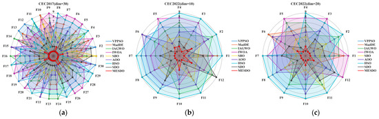
Figure 10.
Distribution of rankings of different algorithms.
In summary, the overall ranking data in Table 7 and the function-level ranking distribution in Figure 10 mutually corroborate each other, collectively demonstrating that MESDO not only achieves the best overall performance among eight mainstream algorithms but also exhibits stronger performance stability and smaller ranking fluctuations, providing comprehensive performance support from “overall hierarchy” to “individual functions” for its application in complex optimization problems.
4. Deployment of Wireless Sensor Network Problems
4.1. WSN Mathematical Model
The perception model of the sensor is shown in Figure 11, where the sensing region and communication range are defined by two concentric circles. The sensing area is modeled as a disk with radius , while the communication radius is set to twice (i.e., ). According to existing studies [49,52], when the communication range is at least twice the sensing range, the network can ensure full coverage of the convex area while maintaining connectivity among all active nodes. However, this model is based on the assumption of omnidirectional sensing and is not applicable to devices with directional sensing capabilities, such as cameras or ultrasonic sensors.
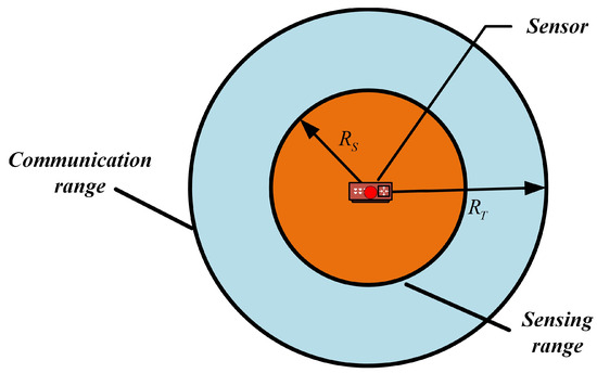
Figure 11.
Perception model of sensor node.
Sensor nodes rely on battery power, and their limited operational lifetime constitutes a core constraint in network deployment. To prolong system lifetime, energy-efficient coverage protocols must be adopted. In wireless sensor networks, there are two mainstream coverage models: one is the binary detection model that ignores uncertainty, and the other is a probabilistic sensing model that incorporates randomness, closer to real-world physics. The probability of an event being detected is inversely proportional to the Euclidean distance between the sensor and the event source. Although the binary model is commonly used in theoretical analyses due to its simplicity (assuming that a sensor can deterministically detect everything within its sensing disk), the probabilistic model better reflects sensor performance in real environments. Based on these considerations, this study adopts the binary detection model proposed in [53,54], defined as follows in Equation (26):
where is the probability that an event occurring at position is detected by a sensor located at , and is the Euclidean distance between the sensor and the event.
The objective function in this study primarily considers coverage. Let sensor nodes be and the deployment space be . The sensor’s coverage radius is , and the covered points are denoted as . The coverage equation is defined as follows [53]:
where is the Euclidean distance from sensor to point , calculated as [53]:
The coverage probability ratio of the deployment area is defined as:
where and are the length and width of the deployment area. The objective of this problem is to maximize network coverage, which constitutes a maximization problem. Therefore, the fitness function is given as [53]:
4.2. WSN Experiment
The experiments were conducted in a 50 × 50 simulation environment, deploying 30 sensor nodes with a communication radius of . To ensure fair comparison, all algorithms used the same fitness function parameters and were independently run 30 times to eliminate randomness. A comprehensive evaluation framework was established, collecting multiple metrics including minimum, maximum, median, mean, standard deviation, p-value, and ranking, with the optimal values highlighted in bold in Table 8. The convergence characteristics and final deployment results are presented in Figure 12 and Figure 13, respectively.
Table 8.
Statistics of WSN experiment results.
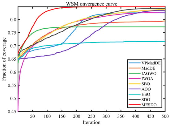
Figure 12.
Fitness value curves of different algorithms in WSN.
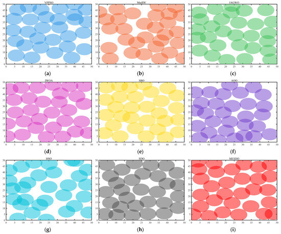
Figure 13.
Node deployment distributions obtained by different algorithms.
Table 8 quantifies the WSN deployment performance of each algorithm using metrics such as minimum coverage (Min), median coverage (Median), maximum coverage (Max), average coverage (Ave), standard deviation (Std), p-value, and ranking. The data show that MESDO achieves the best performance across all metrics: in terms of average coverage, MESDO reaches 86.80%, which is 2.39 percentage points higher than the second-ranked SDO (84.41%), 2.52 and 2.71 percentage points higher than IWOA (84.28%) and HSO (84.09%), respectively, and exceeds AOO (71.71%) and MadDE (77.40%) by more than 15 percentage points; for minimum coverage, MESDO achieves 84.80%, significantly higher than SDO (81.24%) and IWOA (82.48%), and 21.21 percentage points higher than AOO (69.96%), demonstrating that MESDO maintains high coverage even in the worst deployment scenarios; in terms of median coverage, MESDO reaches 86.90%, 2.26 percentage points higher than SDO (84.64%), while all other compared algorithms have median coverage below 85%, further highlighting MESDO’s superiority. Meanwhile, MESDO’s standard deviation is only 8.1308 × 10³, lower than SDO (1.2635 × 10²) and IWOA (8.8350 × 10³), indicating minimal fluctuation across 30 independent runs and excellent stability. The p-value results show that MESDO’s performance differences with all other algorithms are statistically significant (all other algorithms have p-values far below 0.05), ultimately securing the top ranking with absolute advantage.
Figure 12 presents the fitness value curves (with coverage as the core fitness metric), providing a dynamic convergence perspective that further confirms the quantitative conclusions in Table 8: during the early iterations (1–50 generations), MESDO’s fitness rapidly rises above 82%, with convergence significantly faster than other algorithms—SDO requires 80 generations to reach 82%, IWOA and HSO around 100 generations, while AOO, MadDE, VPPSO, and others still remain below 80% at 100 generations; in the middle iterations (50–200 generations), MESDO’s fitness steadily increases from 82% to 86% without noticeable stagnation, whereas SDO, IWOA, and other algorithms enter a slow-convergence phase, with coverage improvement less than 2 percentage points, and AOO and MadDE even exhibit stagnation; in the late iterations (200–500 generations), MESDO’s fitness stabilizes around 86.80%, reaching convergence, while the final coverage of other algorithms remains below 85%, with AOO only stabilizing around 71.71%, showing a significant gap. This convergence difference stems from the targeted roles of MESDO’s three core strategies in WSN deployment: the elite-guided search strategy quickly locks high-coverage node deployment patterns via a dynamic elite pool, accelerating early-stage convergence; the adaptive differential evolution operator strategy prevents the algorithm from falling into “local optimal deployments” (e.g., clustered nodes creating coverage blind spots), ensuring continued coverage improvement in the mid-stage; the centroid-based opposite learning boundary control strategy adjusts out-of-bound nodes, maintains population diversity, and guarantees stable convergence to the optimal deployment in the late stage.
Figure 13 shows the node deployment distribution, visually highlighting MESDO’s deployment advantages from a practical application perspective: the nodes generated by MESDO are evenly distributed and densely cover the entire 50 × 50 simulation area, with no obvious coverage blind spots, and inter-node distances are reasonable (mostly within the effective communication radius ). This arrangement avoids resource waste caused by excessive node clustering while preventing coverage gaps from overly sparse placement. In contrast, the deployment results of other algorithms exhibit clear deficiencies: VPPSO and MadDE produce scattered node distributions, with dense overlaps in some areas and large coverage blind spots at the edges of the simulation region; IAGWO and IWOA have relatively uniform overall distributions but still show small blind spots in corner areas, and inter-node communication stability is insufficient; SDO, as the original algorithm, performs better than most comparison algorithms but still suffers from local node clustering and lower coverage than MESDO; AOO exhibits the worst distribution, with many nodes concentrated at the center and almost no coverage at the edges, leading to a significantly reduced overall coverage. These deployment differences fundamentally reflect MESDO’s ability to optimize “node placement rationality” and “coverage completeness,” further validating the reliability of the quantitative data in Table 7 and the convergence curves in Figure 12—MESDO not only achieves superior numerical metrics but also generates better node distribution schemes in actual WSN deployments, satisfying the core requirements of network coverage and connection stability.
In summary, Table 8, Figure 12 and Figure 13 collectively corroborate MESDO’s superiority in WSN node deployment optimization across three dimensions: quantitative statistics, dynamic convergence, and practical deployment. MESDO outperforms eight mainstream comparison algorithms in terms of higher coverage accuracy, faster convergence, stronger performance stability, and the ability to generate more uniform, blind-spot-free node deployment schemes, providing a practical and effective optimization method for efficient WSN deployment.
5. Summary and Prospect
This paper addresses the optimization requirements for wireless sensor network (WSN) deployment, focusing on the limitations of the traditional Supply-Demand Optimization (SDO) algorithm, including blind search, weak global exploration, and coarse boundary handling. We propose a Multi-strategy Enhanced Supply-Demand Optimization (MESDO) algorithm, which synergistically integrates three core strategies: an elite-guided search strategy dynamically constructs an elite pool to guide price equilibrium point selection, addressing the blind search direction issue in SDO; an adaptive differential evolution operator strategy dynamically adjusts the mutation factor and leverages the global best solution to enhance global exploration; and a centroid-based opposite learning boundary control strategy corrects out-of-bound solutions using the population centroid, improving the utilization of effective information. MESDO was validated using the CEC2017 and CEC2022 benchmark test suites. The results demonstrate that MESDO consistently achieves optimal performance across unimodal, multimodal, hybrid, and composite functions, effectively avoiding premature convergence. Statistical tests (Wilcoxon rank-sum test and Friedman test) further confirm the synergistic value of the three strategies, with MESDO achieving the top average ranking in all test scenarios, and its performance advantages are statistically significant.
For engineering application validation, MESDO was applied to WSN node deployment in a 50 × 50 simulation environment. The results show an average coverage rate of 86.80%, which is 2.39 percentage points higher than SDO (84.41%); the minimum coverage rate reaches 84.80%, 21.21 percentage points higher than AOO (69.96%); and the standard deviation of 8.1308 × 10³ is lower than all comparison algorithms, indicating superior and more stable deployment performance. Convergence curves reveal that MESDO achieves 82% coverage within 50 iterations, significantly faster than SDO (80 iterations) and IWOA (100 iterations). The node deployment distribution map intuitively shows that MESDO generates a uniform deployment with no noticeable coverage blind spots, effectively avoiding the clustering or sparse placement problems observed in other algorithms (e.g., VPPSO, AOO), fully demonstrating MESDO’s practical value in real-world engineering scenarios.
Compared to existing multi-strategy optimization algorithms in WSN deployment (such as AHDGWO integrated with differential evolution and NHBBWO incorporating dynamic parameters), MESDO’s unique advantage lies in its targeted design of synergistic strategies: while AHDGWO enhances local exploitation, its reliance on a single hybrid strategy constrains global exploration; NHBBWO’s dynamic parameter adjustment is only effective for specific scenarios. In contrast, MESDO achieves three-layer strategy synergy through “elite guidance (precise positioning)—adaptive differential evolution (global expansion)—centroid-based boundary control (diversity stabilization)”. This approach not only resolves the imbalance in traditional multi-strategy algorithms that either overemphasize local optimization at the expense of global search or prioritize exploration over stability, but also ensures consistent performance transfer from function optimization to engineering deployment. Its adaptability to complex functions demonstrated in CEC benchmark tests directly translates into precise optimization of coverage blind spots and convergence speed in WSN deployment—a dual capability rarely achieved by most existing algorithms.
Although MESDO has achieved remarkable results in function optimization and WSN deployment, integrating research findings with practical requirements suggests three potential directions for future research: (1) Extending multi-objective optimization capabilities: Introduce classical non-dominated sorting mechanisms such as the Non-dominated Sorting Genetic Algorithm II (NSGA-II) to construct a multi-objective optimization framework that balances coverage rate, node energy consumption, network connectivity, and other multi-objective requirements in WSNs, thereby addressing the limitations of single-objective optimization in handling multiple engineering constraints; (2) Enhancing adaptability to dynamic and 3D scenarios: Develop dynamic population update strategies (e.g., population reconstruction mechanisms based on environmental changes) and 3D boundary models to accommodate dynamic scenarios such as node mobility and failure, as well as three-dimensional deployment environments like mountainous areas and buildings, thereby improving the algorithm’s applicability in complex real-world scenarios; (3) Exploring cross-domain applications: Apply MESDO to fields such as microgrid scheduling (optimizing energy distribution efficiency) and image segmentation (improving segmentation accuracy and speed) to further validate the algorithm’s generality. Meanwhile, strategy details (e.g., adjusting the mutation factor range in differential evolution, optimizing the elite pool update frequency) should be refined according to the characteristics of different domain problems to promote the algorithm’s practical implementation in engineering.
Author Contributions
Conceptualization, B.W. and Y.Y. (Yuchen Yan); Methodology, B.W. and Y.Y. (Yuchen Yan); Software, B.W. and Y.Y. (Yuchen Yan).; Validation, B.W. and Y.Y. (Yuchen Yan); Formal analysis, B.W. and Y.Y. (Yuchen Yan); Investigation, L.Z. and S.Y.; Resources, L.Z. and S.Y.; Data curation, L.Z. and S.Y.; Writing—original draft, L.Z. and S.Y.; Writing—review and editing, L.Z. and S.Y.; Visualization, Y.Y. (Yangjian Yang); Supervision, Y.Y. (Yangjian Yang); Project administration, Y.Y. (Yangjian Yang). All authors have read and agreed to the published version of the manuscript.
Funding
This research received no external funding.
Data Availability Statement
The original contributions presented in this study are included in the article. Further inquiries can be directed to the corresponding author.
Conflicts of Interest
The authors declare no conflicts of interest.
References
- Uthayakumar, C.; Jayaraman, R.; Raja, H.A.; Shabbir, N. QSEER-Quantum-Enhanced Secure and Energy-Efficient Routing Protocol for Wireless Sensor Networks (WSNs). Sensors 2025, 25, 5924. [Google Scholar] [CrossRef]
- Shafik, W. Wireless sensor network-assisted fuzzy sink based model. Energy 2025, 333, 37512. [Google Scholar] [CrossRef]
- Karunkuzhali, D.; Pradeep, S.; Sungheetha, A.; Basha, T.S.G. Data-Aggregation-Aware Energy-Efficient in Wireless Sensor Networks Using Multi-Stream General Adversarial Network. Trans. Emerg. Telecommun. Technol. 2025, 36, e70017. [Google Scholar] [CrossRef]
- Suganthi, S.; Umapathi, N.; Venkateswaran, N.; Rajarajan, S. Enhancing energy efficiency in wireless sensor networks via predictive model for node status classification and coverage integrity using relational Bi-level aggregation graph convolutional network. Expert Syst. Appl. 2025, 296, 129029. [Google Scholar] [CrossRef]
- Perez, J.; Santamaria, I.; Pagés-Zamora, A. Blind learning of the optimal fusion rule in wireless sensor networks. Signal Process. 2025, 239, 110238. [Google Scholar] [CrossRef]
- Lian, J.; Yao, H. Joint Deployment of Sensors and Chargers in Wireless Rechargeable Sensor Networks. Energies 2024, 17, 3130. [Google Scholar] [CrossRef]
- Lai, W.-Y.; Hsiang, T.-R. Wireless Charging Deployment in Sensor Networks. Sensors 2019, 19, 201. [Google Scholar] [CrossRef] [PubMed]
- Zhang, C.; Zhao, G. Wireless Powered Sensor Networks With Random Deployments. IEEE Wirel. Commun. Lett. 2017, 6, 218–221. [Google Scholar] [CrossRef]
- Kundu, M.; Kanjilal, R.; Uysal, I. Intelligent Clustering and Adaptive Energy Management in Wireless Sensor Networks with KDE-Based Deployment. Sensors 2025, 25, 2588. [Google Scholar] [CrossRef]
- Di Puglia Pugliese, L.; Guerriero, F.; Mitton, N. Optimizing wireless sensor networks deployment with coverage and con-nectivity requirements. Ann. Oper. Res. 2025, 346, 1997–2008. [Google Scholar] [CrossRef]
- Zhou, P.; Kan, M.; Chen, W.; Wang, Y.; Cao, B. An adaptive coverage method for dynamic wireless sensor network deployment using deep reinforcement learning. Sci. Rep. 2025, 15, 30304. [Google Scholar] [CrossRef]
- Xing, Y.-X.; Wang, J.-S.; Zhang, S.-W.; Zhang, S.-H.; Ma, X.-R.; Zhang, Y.-H. Transit search algorithm based on oscillation exploitation factor and Roche limit for wireless sensor network deployment optimization. Artif. Intell. Rev. 2024, 58, 29. [Google Scholar] [CrossRef]
- Zhu, J.; Rong, J.; Gong, Z.; Liu, Y.; Li, W.; Alqahtani, F.; Tolba, A.; Hu, J. Deployment optimization in wireless sensor networks using advanced artificial bee colony algorithm. Peer-to-Peer Netw. Appl. 2024, 17, 3571–3582. [Google Scholar] [CrossRef]
- Niu, H.; Li, Y.; Zhang, C.; Chen, T.; Sun, L.; Abdullah, M.I. Multi-Strategy Bald Eagle Search Algorithm Embedded Orthogonal Learning for Wireless Sensor Network (WSN) Coverage Optimization. Sensors 2024, 24, 6794. [Google Scholar] [CrossRef]
- Kennedy, J.; Eberhart, R. Particle swarm optimization. In Proceedings of the ICNN’95—International Conference on Neural Networks, Perth, WA, Australia, November 27–December 1 1995; Volume 4, pp. 1942–1948. [Google Scholar]
- Dorigo, M.; Birattari, M.; Stützle, T. Ant Colony Optimization. Comput. Intell. Mag. IEEE 2006, 1, 28–39. [Google Scholar] [CrossRef]
- Mirjalili, S.; Mirjalili, S.M.; Lewis, A. Grey Wolf Optimizer. Adv. Eng. Softw. 2014, 69, 46–61. [Google Scholar] [CrossRef]
- Mirjalili, S.; Lewis, A. The Whale Optimization Algorithm. Adv. Eng. Softw. 2016, 95, 51–67. [Google Scholar] [CrossRef]
- Hashim, F.A.; Hussien, A.G. Snake Optimizer: A novel meta-heuristic optimization algorithm. Knowl.-Based Syst. 2022, 242, 108320. [Google Scholar] [CrossRef]
- Xue, J.; Shen, B. A novel swarm intelligence optimization approach: Sparrow search algorithm. Syst. Sci. Control Eng. 2020, 8, 22–34. [Google Scholar] [CrossRef]
- Fu, Y.; Liu, D.; Chen, J.; He, L. Secretary bird optimization algorithm: A new metaheuristic for solving global optimization problems. Artif. Intell. Rev. 2024, 57, 123. [Google Scholar] [CrossRef]
- Saremi, S.; Mirjalili, S.; Lewis, A. Grasshopper Optimisation Algorithm: Theory and application. Adv. Eng. Softw. 2017, 105, 30–47. [Google Scholar] [CrossRef]
- Jia, H.; Peng, X.; Lang, C. Remora optimization algorithm. Expert Syst. Appl. 2021, 185, 115665. [Google Scholar] [CrossRef]
- Gao, Y.; Wang, J.; Li, C. Escape after love: Philoponella prominens optimizer and its application to 3D path planning. Clust. Comput. 2024, 28, 81. [Google Scholar] [CrossRef]
- Hayyolalam, V.; Kazem, A.A.P. Black Widow Optimization Algorithm: A novel meta-heuristic approach for solving engineering optimization problems. Eng. Appl. Artif. Intell. 2020, 87, 103249. [Google Scholar] [CrossRef]
- Xue, J.; Shen, B. Dung beetle optimizer: A new meta-heuristic algorithm for global optimization. J. Supercomput. 2022, 79, 7305–7336. [Google Scholar] [CrossRef]
- Ghasemi, M.; Khodadadi, N.; Trojovský, P.; Li, L.; Mansor, Z.; Abualigah, L.; Alharbi, A.H.; El-Kenawy, E.-S.M. Kirchhoff’s law algorithm (KLA): A novel physics-inspired non-parametric metaheuristic algorithm for optimization problems. Artif. Intell. Rev. 2025, 58, 325. [Google Scholar] [CrossRef]
- Yuting, Y.; Yuelin, G. An adaptive hybrid differential Grey Wolf Optimization algorithm for WSN coverage. Clust. Comput. 2025, 28, 229. [Google Scholar] [CrossRef]
- Chen, X.; Zhang, M.; Yang, M.; Wang, D. NHBBWO: A novel hybrid butterfly-beluga whale optimization algorithm with the dynamic strategy for WSN coverage optimization. Peer-to-Peer Netw. Appl. 2025, 18, 80. [Google Scholar] [CrossRef]
- Zhang, Y.; Zhang, Z.; Liu, D.; Zheng, P.; Zhong, Z. Adaptive learning FOA algorithm with energy consumption balancing for coverage optimization in WSNs. Ad Hoc Netw. 2025, 178, 103958. [Google Scholar] [CrossRef]
- Zhaohui, Z.; Jiaqi, Z.; Jing, L. Q-learning-based semi-fixed clustering routing algorithm in WSNs. Ad Hoc Netw. 2025, 174, 103837. [Google Scholar] [CrossRef]
- Liu, X.; Zhang, K.; Zhang, X.; Fiumara, G.; De Meo, P. A hybrid improved compressed particle swarm optimization WSN node location algorithm. Phys. Commun. 2024, 67, 102490. [Google Scholar] [CrossRef]
- Wang, J.; Zhu, Z.; Zhang, F.; Liu, Y. An improved salp swarm algorithm for solving node coverage optimization problem in WSN. Peer-to-Peer Netw. Appl. 2024, 17, 1091–1102. [Google Scholar] [CrossRef]
- Zhao, W.; Wang, L.; Zhang, Z. Supply-Demand-Based Optimization: A Novel Economics-Inspired Algorithm for Global Optimization. IEEE Access 2019, 7, 73182–73206. [Google Scholar] [CrossRef]
- Daqaq, F.; Hassan, M.H.; Kamel, S.; Hussien, A.G. A leader supply-demand-based optimization for large scale optimal power flow problem considering renewable energy generations. Sci. Rep. 2023, 13, 14591. [Google Scholar] [CrossRef]
- Ginidi, A.R.; Shaheen, A.M.; El-Sehiemy, R.A.; Elattar, E. Supply demand optimization algorithm for parameter extraction of various solar cell models. Energy Rep. 2021, 7, 5772–5794. [Google Scholar] [CrossRef]
- Yin, P.; Luo, Z.; Pouramini, S. Case study on multi-objective Modified Supply-Demand-based Optimization Algorithm for energy-efficient building retrofitting. Sustain. Cities Soc. 2024, 114, 105734. [Google Scholar] [CrossRef]
- Wu, G.; Mallipeddi, R.; Suganthan, P. Problem Definitions and Evaluation Criteria for the CEC 2017 Competition and Special Session on Constrained Single Objective Real-Parameter Optimization; Elsevier: Amsterdam, The Netherlands, 2016. [Google Scholar]
- Luo, W.; Lin, X.; Li, C.; Yang, S.; Shi, Y. Benchmark functions for CEC 2022 competition on seeking multiple optima in dynamic environments. arXiv 2022, arXiv:2201.00523. [Google Scholar] [CrossRef]
- Shami, T.M.; Mirjalili, S.; Al-Eryani, Y.; Daoudi, K.; Izadi, S.; Abualigah, L. Velocity pausing particle swarm optimization: A novel variant for global optimization. Neural Comput. Appl. 2023, 35, 9193–9223. [Google Scholar] [CrossRef]
- Biswas, S.; Saha, D.; De, S.; Cobb, A.D.; Das, S.; Jalaian, B.A. Improving differential evolution through Bayesian hy-perparameter optimization. In Proceedings of the 2021 IEEE Congress on Evolutionary Computation (CEC), Kraków, Poland, 28 June–1 July 2021; IEEE: New York City, NY, USA, 2021; pp. 832–840. [Google Scholar]
- Yu, M.; Xu, J.; Liang, W.; Qiu, Y.; Bao, S.; Tang, L. Improved multi-strategy adaptive Grey Wolf Optimization for practical engineering applications and high-dimensional problem solving. Artif. Intell. Rev. 2024, 57, 277. [Google Scholar] [CrossRef]
- Huang, S.; Liu, D.; Fu, Y.; Chen, J.; He, L.; Yan, J.; Yang, D. Prediction of Self-Care Behaviors in Patients Using High-Density Surface Electromyography Signals and an Improved Whale Optimization Algorithm-Based LSTM Model. J. Bionic Eng. 2025, 22, 1963–1984. [Google Scholar] [CrossRef]
- Wang, J.; Chen, Y.; Lu, C.; Heidari, A.A.; Wu, Z.; Chen, H. The status-based optimization: Algorithm and comprehensive performance analysis. Neurocomputing 2025, 647, 130603. [Google Scholar] [CrossRef]
- Wang, R.-B.; Hu, R.-B.; Geng, F.-D.; Xu, L.; Chu, S.-C.; Pan, J.-S.; Meng, Z.-Y.; Mirjalili, S. The Animated Oat Optimization Algorithm: A nature-inspired metaheuristic for engineering optimization and a case study on Wireless Sensor Networks. Knowl. -Based Syst. 2025, 318, 113589. [Google Scholar] [CrossRef]
- Akbari, E.; Rahimnejad, A.; Gadsden, S.A. Holistic swarm optimization: A novel metaphor-less algorithm guided by whole population information for addressing exploration-exploitation dilemma. Comput. Methods Appl. Mech. Eng. 2025, 445, 118208. [Google Scholar] [CrossRef]
- Yang, W.; Lai, T.; Fang, Y. Multi-Strategy Golden Jackal Optimization for engineering design. J. Supercomput. 2025, 81, 609. [Google Scholar] [CrossRef]
- Zhang, Y.; Wang, J.; Zhang, X.; Wang, B. ACPOA: An Adaptive Cooperative Pelican Optimization Algorithm for Global Optimization and Multilevel Thresholding Image Segmentation. Biomimetics 2025, 10, 596. [Google Scholar] [CrossRef] [PubMed]
- Wu, Q. An enhanced whale optimization algorithm with inertia weight and dynamic parameter adaptation for wireless sensor network deployment. Computing 2025, 107, 167. [Google Scholar] [CrossRef]
- Cao, L.; Wei, Q. SZOA: An Improved Synergistic Zebra Optimization Algorithm for Microgrid Scheduling and Management. Biomimetics 2025, 10, 664. [Google Scholar] [CrossRef]
- Shen, Y.; Zhang, C.; Gharehchopogh, F.S.; Mirjalili, S. An improved whale optimization algorithm based on multi-population evolution for global optimization and engineering design problems. Expert Syst. Appl. 2022, 215, 119269. [Google Scholar] [CrossRef]
- Wang, Z.; Xie, H. Wireless Sensor Network Deployment of 3D Surface Based on Enhanced Grey Wolf Optimizer. IEEE Access 2020, 8, 57229–57251. [Google Scholar] [CrossRef]
- Meng, Q.; Kuang, X.; Yu, Z.; He, M.; Cui, H. Augmented secretary bird optimization algorithm for wireless sensor network deployment and engineering problem. PLoS ONE 2025, 20, e0329705. [Google Scholar] [CrossRef]
- Wang, W.; Lyu, L. Adaptive Tasmanian Devil Optimizer for Global Optimization and Application in Wireless Sensor Network Deployment. IEEE Access 2024, 12, 72382–72407. [Google Scholar] [CrossRef]
Disclaimer/Publisher’s Note: The statements, opinions and data contained in all publications are solely those of the individual author(s) and contributor(s) and not of MDPI and/or the editor(s). MDPI and/or the editor(s) disclaim responsibility for any injury to people or property resulting from any ideas, methods, instructions or products referred to in the content. |
© 2025 by the authors. Licensee MDPI, Basel, Switzerland. This article is an open access article distributed under the terms and conditions of the Creative Commons Attribution (CC BY) license (https://creativecommons.org/licenses/by/4.0/).