Applications of Fixed-Point Results to Image Processing

Abstract

The primary objective of this study is to establish common fixed-point theorems for single-valued and multivalued mappings in the setting of complex-valued suprametric spaces. A new contraction is introduced for single-valued mappings, while a generalized Hausdorff distance aids in proving results for multivalued mappings. Additionally, fixed-point theorems are extended to complex-valued metric spaces. An example illustrates the findings, and an application to Fredholm integral equations demonstrates their role in image processing.

1. Introduction

Fixed-point (FP) theory is a vast and diverse field with three principal branches: metric, topological, and discrete FP theory. Among these, metric FP theory serves as a foundational pillar, concentrating on proving the existence and uniqueness of FPs for self-mappings defined on metric spaces (MSs). This theory is intrinsically tied to the notions of distance and convergence, which are the defining characteristics of MSs. The concept of an MS, developed by Maurice Fréchet [1] in 1906, establishes a solid foundation for quantifying distances between elements within a set. An MS is formally defined as a set equipped with a distance function, or metric, that satisfies specific axioms such as non-negativity, symmetry, and triangle inequality. Over time, this foundational idea has undergone significant development and generalization, leading to the creation of more complex mathematical structures that extend beyond classical MSs. One of the notable generalizations is the partial metric space (PMS), introduced by Matthews [2], which allows the self-distance of a point to be non-zero. This relaxation of the traditional MS axioms is particularly in areas that deal with computation, semantics, and formal methods. Similarly, Bakhtin [3] introduced b-metric spaces (b-MSs), where the triangle inequality is modified by incorporating a constant factor on the right-hand side. Further generalizations include rectangular metric spaces (RMSs), developed by Branciari [4], where the classical triangle inequality is replaced by a rectangular condition. This modification has found applications in the analysis of nonlinear problems and optimization models. Cone metric spaces (CMSs), introduced by Huang [5], represent a significant generalization of traditional MSs by replacing the real-valued distance function with a metric that takes values within a cone in a Banach space. This innovative approach provides a flexible framework for analyzing FP theorems and solving integral equations in more abstract and generalized mathematical settings. Among the more recent advancements is the concept of supra metric spaces (SMSs), introduced by Berzig [6]. SMSs are characterized by a relaxed version of the triangle inequality, allowing for a broader range of applications. The framework of SMSs has also been applied to nonlinear integral and matrix equations, demonstrating its versatility in addressing complex mathematical challenges. Later on, Berzig [7,8,9] extended the concept of SMS by generalizing the triangle inequality axiom, introducing two new MSs: generalized SMSs and b-SMSs. Additionally, recent studies by Antón-Sancho [10,11,12] further expand the FP theory in more complex and geometric contexts, including the FPs of principal $E_6$-bundles over compact algebraic curves, involutions of G-Higgs bundle moduli spaces over compact Riemann surfaces, and the study of Spin(8,$\mathbb{C}$)-Higgs bundles in relation to the Hitchin integrable system.

On the other hand, the concept of complex-valued metric spaces (C-VMSs) was introduced by Azam et al. [13], emerging as a special case of CMSs and an extension of an MS. C-VMSs extended the classical MSs by considering distance functions that take values in the set of complex numbers $\mathbb{C}$. Rouzkard et al. [14] built upon the work of Azam et al. [13] by incorporating a rational expression into the contractive condition, significantly enhancing the scope of FP theory in C-VMSs. Afterwards, Hussain et al. [15] gave an innovative contractive condition in the background of C-VMSs and presented some common fixed-point (CFP) results. Subsequently, Ahmad et al. [16,17] further strengthened the concept of C-VMSs by developing CFP theorems for multivalued mappings, specifically under generalized contraction conditions. More recently, Panda et al. [18] unified the concepts of supra metric spaces (SMSs) and CVMSs, introducing the novel concept of complex-valued suprametric spaces (C-VSMSs). Within this new framework, they established several CFP theorems for rational contractions and demonstrated their applicability in solving complex nonlinear integral equations using contractive mappings. For readers interested in a detailed exploration of these advancements, further insights can be found in references [19,20,21,22].

FP theory has emerged as a powerful mathematical tool with significant applications in various scientific and engineering disciplines. One of its notable applications is in image processing, particularly in image restoration and enhancement. The use of FP methods in this domain has gained substantial attention due to their robustness, efficiency, and ability to handle complex optimization problems. Several studies have demonstrated the effectiveness of FP methods in image restoration. Hanjing et al. [23] introduced a fast image restoration algorithm that integrates this theory with optimization techniques, showcasing improved computational efficiency. Similarly, Kim et al. [24] employed an FP approach to solve a total variation $L_2(TVL2)$ regularization problem, which plays a crucial role in reducing noise while preserving important image features. FP methodologies have also been successfully implemented in hardware-based image processing. Cabello et al. [25] designed an FP 2D Gaussian filter for image processing using field-programmable gate arrays (FPGAs), highlighting the applicability of FP arithmetic in real-time signal processing tasks. Furthermore, Mishra et al. [26] explored contraction mapping principles in digital image processing, demonstrating their relevance in improving image reconstruction techniques. In particular, image denoising has become a central problem in medical imaging, where noisy CT, MRI, X-ray, and ultrasound scans can lead to misdiagnosis. Recent survey work of Kaur et al. [27] provides a comprehensive overview of state-of-the-art denoising techniques, including filtering methods, CNN-based approaches, GAN-based strategies, and Transformer-based frameworks. While such methods rely on machine learning and optimization strategies, FP theory provides a rigorous mathematical foundation for iterative schemes that underpin many of these algorithms.

On the other hand, FP theorems are a cornerstone of functional analysis, offering a robust framework for establishing the existence and uniqueness of solutions to a wide range of mathematical equations, including integral equations. Their significance is particularly evident in tackling intricate problems such as Fredholm integral equations, where FP theorems provide a structured approach to proving solvability and guaranteeing uniqueness under specific conditions. Fredholm integral equations are fundamental in numerous applied domains, including image processing (image deblurring and image denoising), where they serve as a crucial tool for modeling and solving various inverse problems. For further information, readers are encouraged to consult references [28,29,30].

In this study, we investigate the concept of C-VSMSs and establish CFP theorems for single-valued mappings under generalized contractions. Additionally, the study introduces the concept of generalized Hausdorff distance function to obtain FP theorems for multivalued mappings in the context of C-VSMSs. These theoretical advancements apply directly to C-VMSs and SMSs, leading to the derivation of some FP theorems as natural consequences of our leading results. To highlight the relevance and originality of our results, an example is provided to illustrate the main findings. We further examine the practical application of these results by applying them to the solution of Fredholm integral equations, which are significant in image denoising.

2. Preliminaries

In this section, we present the fundamental definitions, notations, and essential results that form the basis for our main findings. Since our main results are established in C-VSMSs, we first introduce the notions of MSs, SMSs, and C-VMSs to provide a structured foundation. Additionally, we review key properties related to contractions, completeness, and convergence, ensuring a self-contained framework for our FP results. These preliminaries will be instrumental in formulating and proving the main theorems in subsequent sections.

The concept of MS was introduced by Fréchet [1] in 1906, defined as follows:

Definition 1 

([1]). Let $\mathcal{N}\ne Ø$ and $d:\mathcal{N}\times \mathcal{N}\to {\mathbb{R}}^{+}$ be a function that fulfills the following axioms:

(i) 

$0\le d(\mathfrak{l},\varsigma )$ and $d(\mathfrak{l},\varsigma )=0$ ⇔ $\mathfrak{l}=\varsigma$;

(ii) 

$d(\mathfrak{l},\varsigma )=d(\varsigma ,\mathfrak{l});$

(iii) 

$d(\mathfrak{l},\varsigma )\le d(\mathfrak{l},\nu )+d(\nu ,\varsigma );$

for all $\mathfrak{l},\varsigma ,\nu \in \mathcal{N};$ then $(\mathcal{N},d)$ is called an MS.

Berzig [6] introduced the concept of SMS in this way.

Definition 2 

([6]). Let $\mathcal{N}\ne Ø$ and ⋏ be a non-negative real constant. Consider a function $d:\mathcal{N}\times \mathcal{N}\to {\mathbb{R}}^{+}$ that satisfies the following properties:

(i) 

$0\le d(\mathfrak{l},\varsigma )$ and $d(\mathfrak{l},\varsigma )=0$ ⇔ $\mathfrak{l}=\varsigma$;

(ii) 

$d(\mathfrak{l},\varsigma )=d(\varsigma ,\mathfrak{l});$

(iii) 

$d(\mathfrak{l},\varsigma )\le d(\mathfrak{l},\nu )+d(\nu ,\varsigma )+⋏d(\mathfrak{l},\nu )d(\nu ,\varsigma );$

for all $\mathfrak{l},\varsigma ,\nu \in \mathcal{N};$ then $(\mathcal{N},d)$ is called an SMS.

Example 1. 

Let $\mathcal{N}=\left\{0,1,2\right\}.$ Define the function $d:\mathcal{N}\times \mathcal{N}\to {\mathbb{R}}^{+}$ as follows:

$$d(0,1)=d(1,0)=0.5$$

$$d(0,2)=d(2,0)=1$$

$$d(1,2)=d(2,1)=2,$$

and

$$d(0,0)=d(1,1)=d(2,2)=0.$$

Let us choose $⋏=1.$ Then $\left(\mathcal{N},d\right)$ is an SMS but not an MS because the triangle of MS is not satisfied; that is,

$$2=d(1,2)>d(1,0)+d(0,2)=0.5+1.$$

The concept of a partial order $\precsim$ on the set $\mathbb{C}$ is introduced as follows:

$$z_1\precsim z_2\iff Re\left(z_1\right)⩽Re\left(z_2\right),Im\left(z_1\right)⩽Im\left(z_2\right).$$

for all $z_1,z_2\in \mathbb{C}.$ It follows that

$$z_1\precsim z_2$$

if one of these conditions is met:

$$\begin{array}{ccc}\hfill (a)Re\left(z_1\right)& =& Re\left(z_2\right),Im\left(z_1\right)<Im\left(z_2\right),\hfill \\ \hfill (b)Re\left(z_1\right)& <& Re\left(z_2\right),Im\left(z_1\right)=Im\left(z_2\right),\hfill \\ \hfill (c)Re\left(z_1\right)& <& Re\left(z_2\right),Im\left(z_1\right)<Im\left(z_2\right),\hfill \\ \hfill (d)Re\left(z_1\right)& =& Re\left(z_2\right),Im\left(z_1\right)=Im\left(z_2\right).\hfill \end{array}$$

Azam et al. [13] defined the concept of CVMS as follows:

Definition 3 

([13]). Let $\mathcal{N}\ne Ø$ and $d:\mathcal{N}\times \mathcal{N}\to \mathbb{C}$ be a function that satisfies the subsequent axioms:

(i) 

$0\precsim d(\mathfrak{l},\varsigma )$ and $d(\mathfrak{l},\varsigma )=0$ ⇔ $\mathfrak{l}=\varsigma$;

(ii) 

$d(\mathfrak{l},\varsigma )=d(\varsigma ,\mathfrak{l});$

(iii) 

$d(\mathfrak{l},\varsigma )\precsim d(\mathfrak{l},\nu )+d(\nu ,\varsigma );$

for all $\mathfrak{l},\varsigma ,\nu \in \mathcal{N}$; then $(\mathcal{N},d)$ is said to be a CVMS.

Example 2 

([13]). Let $\mathcal{N}=[0,1]$ and $\mathfrak{l},\varsigma \in \mathcal{N}.$ Define $d:\mathcal{N}\times \mathcal{N}\to \mathbb{C}$ by

$$d(\mathfrak{l},\varsigma )=\left\{\begin{array}{c}0,\mathit{if}\mathfrak{l}=\varsigma ,\\ {\displaystyle \frac{i}{2}},\mathit{if}\mathfrak{l}\ne \varsigma .\end{array}\right.$$

Then $(\mathcal{N},d)$ is a CVMS.

Very recently, Panda et al. [18] defined the notion of C-VSMS in this manner.

Definition 4 

([18]). Let $\mathcal{N}\ne Ø,$ $⋏\ge 0$ and $d:\mathcal{N}\times \mathcal{N}\to \mathbb{C}$ be a mapping satisfying

(i) 

$0\precsim d(\mathfrak{l},\varsigma )$ and $d(\mathfrak{l},\varsigma )=0$ ⇔ $\mathfrak{l}=\varsigma$;

(ii) 

$d(\mathfrak{l},\varsigma )=d(\varsigma ,\mathfrak{l});$

(iii) 

$d(\mathfrak{l},\varsigma )\precsim d(\mathfrak{l},\nu )+d(\nu ,\varsigma )+⋏d(\mathfrak{l},\nu )d(\nu ,\varsigma );$

for all $\mathfrak{l},\varsigma ,\nu \in \mathcal{N};$ then $(\mathcal{N},d)$ is considered as C-VSMS.

Example 3. 

Let $\mathcal{N}=\{0,1,2\}$ and $d:\mathcal{N}\times \mathcal{N}\to \mathbb{C}$ is defined as

$$d(\mathfrak{l},\varsigma )=\left\{\begin{array}{c}0,\mathit{if}\mathfrak{l}=\varsigma ,\\ 1+i,\mathit{if}\mathfrak{l}\ne \varsigma ,\end{array}\right.$$

for all $\mathfrak{l},\varsigma \in \mathcal{N}$. Then ($\mathcal{N}$,d) is a C-VSMS with $⋏=1$.

Remark 1. 

By setting ⋏ to zero in Definition 4, the idea of C-VSMS is simplified to C-VMS.

Lemma 1 

([18]). Let $(\mathcal{N},d)$ be a C-VSMS and let $\left\{{\mathfrak{l}}_n\right\}$ $\subseteq \mathcal{N}$. Then $\left\{{\mathfrak{l}}_n\right\}$ converges to $\mathfrak{l}$ if and only if $\left|d({\mathfrak{l}}_n,\mathfrak{l})\right|\to 0$ as $n\to \infty .$

Lemma 2 

([18]). Let $(\mathcal{N},d)$ be a C-VSMS and let $\left\{{\mathfrak{l}}_n\right\}$ $\subseteq \mathcal{N}$. Then $\left\{{\mathfrak{l}}_n\right\}$ is a Cauchy sequence if and only if $\left|d({\mathfrak{l}}_n,{\mathfrak{l}}_{n+m})\right|\to 0$ as $n\to \infty ,$ where $m\in \mathbb{N}.$

3. Main Results

In this section, we establish CFP theorems for self mappings in the setting of C-VSMSs. Building on the preliminaries introduced earlier, we state and prove new FP results under generalized contractive conditions. These theorems generalize and extend existing results in C-VMSs and SMSs. The findings contribute to the broader study of FP theory in generalized metric structures and provide a theoretical foundation for potential applications in nonlinear analysis and integral equations.

Theorem 1. 

Let $(\mathcal{N},d)$ be a complete C-VSMS and consider mappings $\mathcal{R},\mathfrak{J}:\mathcal{N}\to \mathcal{N}$. Suppose that there is a constant $\varpi \in [0,1)$ such that

$$d(\mathcal{R}\mathfrak{l},\mathfrak{J}\varsigma )⪯\varpi \mathcal{M}(\mathfrak{l},\varsigma ),$$

(1)

where

$$\mathcal{M}(\mathfrak{l},\varsigma )=\left\{d(\mathfrak{l},\varsigma ),d(\mathfrak{l},\mathcal{R}\mathfrak{l}),d(\varsigma ,\mathfrak{J}\varsigma ),{\displaystyle \frac{d(\mathfrak{l},\mathcal{R}\mathfrak{l})d(\varsigma ,\mathfrak{J}\varsigma )}{1+d(\mathfrak{l},\varsigma )}}\right\},$$

(2)

holds for all $\mathfrak{l},\varsigma \in \mathcal{N}$. Then $\mathcal{R}$ and $\mathfrak{J}$ possess a unique CFP.

Proof. 

Let ${\mathfrak{l}}_0\in \mathcal{N}$ be given. Define the sequence {${\mathfrak{l}}_n$} inductively by

$${\mathfrak{l}}_{2n+1}=\mathcal{R}{\mathfrak{l}}_{2n}\mathrm{and}{\mathfrak{l}}_{2n+2}={\mathfrak{Jl}}_{2n+1}$$

for all $n\in \mathbb{N},$ where $\mathcal{R},\mathfrak{J}:\mathcal{N}\to \mathcal{N}$ are the self mappings. By (1) and (2), we have

$$d({\mathfrak{l}}_{2n+1},{\mathfrak{l}}_{2n+2})=d(\mathcal{R}{\mathfrak{l}}_{2n},{\mathfrak{Jl}}_{2n+1})⪯\varpi \mathcal{M}({\mathfrak{l}}_{2n},{\mathfrak{l}}_{2n+1}),$$

(3)

where

$$\mathcal{M}({\mathfrak{l}}_{2n},{\mathfrak{l}}_{2n+1})=\left\{\begin{array}{c}d({\mathfrak{l}}_{2n},{\mathfrak{l}}_{2n+1}),d({\mathfrak{l}}_{2n},\mathcal{R}{\mathfrak{l}}_{2n}),d({\mathfrak{l}}_{2n+1},{\mathfrak{Jl}}_{2n+1}),\\ {\displaystyle \frac{d({\mathfrak{l}}_{2n},\mathcal{R}{\mathfrak{l}}_{2n})d({\mathfrak{l}}_{2n+1},{\mathfrak{Jl}}_{2n+1})}{1+d({\mathfrak{l}}_{2n},{\mathfrak{l}}_{2n+1})}}\end{array}\right\}.$$

If $\mathcal{M}({\mathfrak{l}}_{2n},{\mathfrak{l}}_{2n+1})=d({\mathfrak{l}}_{2n},{\mathfrak{l}}_{2n+1}),$ then from (3), we have

$$d({\mathfrak{l}}_{2n+1},{\mathfrak{l}}_{2n+2})⪯\varpi d({\mathfrak{l}}_{2n},{\mathfrak{l}}_{2n+1}),$$

for all $n\in \mathbb{N},$ which implies that

$$\left|d({\mathfrak{l}}_{2n+1},{\mathfrak{l}}_{2n+2})\right|\le \varpi \left|d({\mathfrak{l}}_{2n},{\mathfrak{l}}_{2n+1})\right|,$$

for all $n\in \mathbb{N}.$ If $\mathcal{M}({\mathfrak{l}}_{2n},{\mathfrak{l}}_{2n+1})=d({\mathfrak{l}}_{2n},\mathcal{R}{\mathfrak{l}}_{2n}),$ then from (3), we have

$$d({\mathfrak{l}}_{2n+1},{\mathfrak{l}}_{2n+2})⪯\varpi d({\mathfrak{l}}_{2n},\mathcal{R}{\mathfrak{l}}_{2n})=\varpi d({\mathfrak{l}}_{2n},{\mathfrak{l}}_{2n+1}),$$

signifying that

$$\left|d({\mathfrak{l}}_{2n+1},{\mathfrak{l}}_{2n+2})\right|\le \varpi \left|d({\mathfrak{l}}_{2n},{\mathfrak{l}}_{2n+1})\right|,$$

for all $n\in \mathbb{N}.$ If $\mathcal{M}({\mathfrak{l}}_{2n},{\mathfrak{l}}_{2n+1})=d({\mathfrak{l}}_{2n+1},{\mathfrak{Jl}}_{2n+1}),$ then from (3), we have

$$d({\mathfrak{l}}_{2n+1},{\mathfrak{l}}_{2n+2})⪯\varpi d({\mathfrak{l}}_{2n+1},{\mathfrak{Jl}}_{2n+1})=\varpi d({\mathfrak{l}}_{2n+1},{\mathfrak{l}}_{2n+2})$$

which yields that

$$\left|d({\mathfrak{l}}_{2n+1},{\mathfrak{l}}_{2n+2})\right|\le \varpi \left|d({\mathfrak{l}}_{2n+1},{\mathfrak{l}}_{2n+2})\right|<\left|d({\mathfrak{l}}_{2n+1},{\mathfrak{l}}_{2n+2})\right|,$$

and because $\varpi <1,$ we get a contradiction. Hence $\mathcal{M}({\mathfrak{l}}_{2n},{\mathfrak{l}}_{2n+1})\ne d({\mathfrak{l}}_{2n+1},{\mathfrak{Jl}}_{2n+1}).$ Now if

$$\mathcal{M}({\mathfrak{l}}_{2n},{\mathfrak{l}}_{2n+1})={\displaystyle \frac{d({\mathfrak{l}}_{2n},\mathcal{R}{\mathfrak{l}}_{2n})d({\mathfrak{l}}_{2n+1},{\mathfrak{Jl}}_{2n+1})}{1+d({\mathfrak{l}}_{2n},{\mathfrak{l}}_{2n+1})}},$$

then from (3), we have

$$\begin{array}{ccc}\hfill d({\mathfrak{l}}_{2n+1},{\mathfrak{l}}_{2n+2})& ⪯& \varpi {\displaystyle \frac{d({\mathfrak{l}}_{2n},\mathcal{R}{\mathfrak{l}}_{2n})d({\mathfrak{l}}_{2n+1},{\mathfrak{Jl}}_{2n+1})}{1+d({\mathfrak{l}}_{2n},{\mathfrak{l}}_{2n+1})}}\hfill \\ & =& \varpi {\displaystyle \frac{d({\mathfrak{l}}_{2n},{\mathfrak{l}}_{2n+1})d({\mathfrak{l}}_{2n+1},{\mathfrak{l}}_{2n+2})}{1+d({\mathfrak{l}}_{2n},{\mathfrak{l}}_{2n+1})}},\hfill \end{array}$$

which implies that

$$\begin{array}{ccc}\hfill \left|d({\mathfrak{l}}_{2n+1},{\mathfrak{l}}_{2n+2})\right|& \le & \varpi {\displaystyle \frac{\left|d({\mathfrak{l}}_{2n},{\mathfrak{l}}_{2n+1})\right|\left|d({\mathfrak{l}}_{2n+1},{\mathfrak{l}}_{2n+2})\right|}{\left|1+d({\mathfrak{l}}_{2n},{\mathfrak{l}}_{2n+1})\right|}}\hfill \\ & \le & \varpi \left|d({\mathfrak{l}}_{2n+1},{\mathfrak{l}}_{2n+2})\right|,\hfill \end{array}$$

because $\left|d({\mathfrak{l}}_{2n},{\mathfrak{l}}_{2n+1})\right|<\left|1+d({\mathfrak{l}}_{2n},{\mathfrak{l}}_{2n+1})\right|$ and ${\displaystyle \frac{\left|d({\mathfrak{l}}_{2n},{\mathfrak{l}}_{2n+1})\right|}{\left|1+d({\mathfrak{l}}_{2n},{\mathfrak{l}}_{2n+1})\right|}}<1.$ But since $\varpi <1,$ so we have

$$\left|d({\mathfrak{l}}_{2n+1},{\mathfrak{l}}_{2n+2})\right|\le \varpi \left|d({\mathfrak{l}}_{2n+1},{\mathfrak{l}}_{2n+2})\right|<\left|d({\mathfrak{l}}_{2n+1},{\mathfrak{l}}_{2n+2})\right|,$$

a contradiction. Hence $\mathcal{M}({\mathfrak{l}}_{2n},{\mathfrak{l}}_{2n+1})\ne {\displaystyle \frac{d({\mathfrak{l}}_{2n},\mathcal{R}{\mathfrak{l}}_{2n})d({\mathfrak{l}}_{2n+1},{\mathfrak{Jl}}_{2n+1})}{1+d({\mathfrak{l}}_{2n},{\mathfrak{l}}_{2n+1})}}.$ Thus from all the cases, we have

$$\left|d({\mathfrak{l}}_{2n+1},{\mathfrak{l}}_{2n+2})\right|\le \varpi \left|d({\mathfrak{l}}_{2n},{\mathfrak{l}}_{2n+1})\right|,$$

(4)

for all $n\in \mathbb{N}.$ Similarly, from (1) and (2), we have

$$\begin{array}{ccc}\hfill d({\mathfrak{l}}_{2n+2},{\mathfrak{l}}_{2n+3})& =& d({\mathfrak{Jl}}_{2n+1},\mathcal{R}{\mathfrak{l}}_{2n+2})\hfill \\ & =& d(\mathcal{R}{\mathfrak{l}}_{2n+2},{\mathfrak{Jl}}_{2n+1})⪯\varpi \mathcal{M}({\mathfrak{l}}_{2n+2},{\mathfrak{l}}_{2n+1}),\hfill \end{array}$$

(5)

where

$$\mathcal{M}({\mathfrak{l}}_{2n+2},{\mathfrak{l}}_{2n+1})=\left\{\begin{array}{c}d({\mathfrak{l}}_{2n+2},{\mathfrak{l}}_{2n+1}),d({\mathfrak{l}}_{2n+2},\mathcal{R}{\mathfrak{l}}_{2n+2}),d({\mathfrak{l}}_{2n+1},{\mathfrak{Jl}}_{2n+1}),\\ {\displaystyle \frac{d({\mathfrak{l}}_{2n+2},\mathcal{R}{\mathfrak{l}}_{2n+2})d({\mathfrak{l}}_{2n+1},{\mathfrak{Jl}}_{2n+1})}{1+d({\mathfrak{l}}_{2n+2},{\mathfrak{l}}_{2n+1})}}\end{array}\right\}.$$

If $\mathcal{M}({\mathfrak{l}}_{2n+2},{\mathfrak{l}}_{2n+1})=d({\mathfrak{l}}_{2n+2},{\mathfrak{l}}_{2n+1}),$ then from (5), we have

$$d({\mathfrak{l}}_{2n+2},{\mathfrak{l}}_{2n+3})⪯\varpi d({\mathfrak{l}}_{2n+2},{\mathfrak{l}}_{2n+3})=\varpi d({\mathfrak{l}}_{2n+1},{\mathfrak{l}}_{2n+2}),$$

for all $n\in \mathbb{N},$ which yields that

$$\left|d({\mathfrak{l}}_{2n+2},{\mathfrak{l}}_{2n+3})\right|\le \varpi \left|d({\mathfrak{l}}_{2n+1},{\mathfrak{l}}_{2n+2})\right|.$$

for all $n\in \mathbb{N}.$ If $\mathcal{M}({\mathfrak{l}}_{2n+2},{\mathfrak{l}}_{2n+1})=d({\mathfrak{l}}_{2n+2},\mathcal{R}{\mathfrak{l}}_{2n+2}),$ then from (5), we have

$$d({\mathfrak{l}}_{2n+2},{\mathfrak{l}}_{2n+3})⪯\varpi d({\mathfrak{l}}_{2n+2},\mathcal{R}{\mathfrak{l}}_{2n+2})=\varpi d({\mathfrak{l}}_{2n+2},{\mathfrak{l}}_{2n+3}),$$

for all $n\in \mathbb{N}.$ It further implies that

$$\left|d({\mathfrak{l}}_{2n+2},{\mathfrak{l}}_{2n+3})\right|\le \varpi \left|d({\mathfrak{l}}_{2n+2},{\mathfrak{l}}_{2n+3})\right|<\left|d({\mathfrak{l}}_{2n+2},{\mathfrak{l}}_{2n+3})\right|,$$

and because $\varpi <1,$ we get a contradiction. Hence $\mathcal{M}({\mathfrak{l}}_{2n+2},{\mathfrak{l}}_{2n+1})\ne d({\mathfrak{l}}_{2n+2},\mathcal{R}{\mathfrak{l}}_{2n+2}),$ for all $n\in \mathbb{N}.$ If $\mathcal{M}({\mathfrak{l}}_{2n+2},{\mathfrak{l}}_{2n+1})=d({\mathfrak{l}}_{2n+1},{\mathfrak{Jl}}_{2n+1}),$ then from (5), we have

$$d({\mathfrak{l}}_{2n+2},{\mathfrak{l}}_{2n+3})⪯\varpi d({\mathfrak{l}}_{2n+1},{\mathfrak{Jl}}_{2n+1})=\varpi d({\mathfrak{l}}_{2n+1},{\mathfrak{l}}_{2n+2}),$$

for all $n\in \mathbb{N}.$ This yields that

$$\left|d({\mathfrak{l}}_{2n+2},{\mathfrak{l}}_{2n+3})\right|\le \varpi \left|d({\mathfrak{l}}_{2n+1},{\mathfrak{l}}_{2n+2})\right|,$$

for all $n\in \mathbb{N}.$ If $\mathcal{M}({\mathfrak{l}}_{2n+2},{\mathfrak{l}}_{2n+1})={\displaystyle \frac{d({\mathfrak{l}}_{2n+2},\mathcal{R}{\mathfrak{l}}_{2n+2})d({\mathfrak{l}}_{2n+1},{\mathfrak{Jl}}_{2n+1})}{1+d({\mathfrak{l}}_{2n+2},{\mathfrak{l}}_{2n+1})}},$ then from (5), we have

$$\begin{array}{ccc}\hfill d({\mathfrak{l}}_{2n+2},{\mathfrak{l}}_{2n+3})& ⪯& \varpi {\displaystyle \frac{d({\mathfrak{l}}_{2n+2},\mathcal{R}{\mathfrak{l}}_{2n+2})d({\mathfrak{l}}_{2n+1},{\mathfrak{Jl}}_{2n+1})}{1+d({\mathfrak{l}}_{2n+2},{\mathfrak{l}}_{2n+1})}}\hfill \\ & =& \varpi {\displaystyle \frac{d({\mathfrak{l}}_{2n+2},{\mathfrak{l}}_{2n+3})d({\mathfrak{l}}_{2n+1},{\mathfrak{l}}_{2n+2})}{1+d({\mathfrak{l}}_{2n+2},{\mathfrak{l}}_{2n+1})}},\hfill \end{array}$$

which implies that

$$\begin{array}{ccc}\hfill \left|d({\mathfrak{l}}_{2n+2},{\mathfrak{l}}_{2n+3})\right|& \le & \varpi {\displaystyle \frac{\left|d({\mathfrak{l}}_{2n+2},{\mathfrak{l}}_{2n+3})\right|\left|d({\mathfrak{l}}_{2n+1},{\mathfrak{l}}_{2n+2})\right|}{\left|1+d({\mathfrak{l}}_{2n+2},{\mathfrak{l}}_{2n+1})\right|}}\hfill \\ & \le & \varpi \left|d({\mathfrak{l}}_{2n+2},{\mathfrak{l}}_{2n+3})\right|,\hfill \end{array}$$

because $\left|d({\mathfrak{l}}_{2n+1},{\mathfrak{l}}_{2n+2})\right|<\left|1+d({\mathfrak{l}}_{2n+2},{\mathfrak{l}}_{2n+1})\right|$ and ${\displaystyle \frac{\left|d({\mathfrak{l}}_{2n+1},{\mathfrak{l}}_{2n+2})\right|}{\left|1+d({\mathfrak{l}}_{2n+2},{\mathfrak{l}}_{2n+1})\right|}}<1.$ But since $\varpi <1,$ so we have

$$\left|d({\mathfrak{l}}_{2n+2},{\mathfrak{l}}_{2n+3})\right|\le \varpi \left|d({\mathfrak{l}}_{2n+2},{\mathfrak{l}}_{2n+3})\right|<\left|d({\mathfrak{l}}_{2n+2},{\mathfrak{l}}_{2n+3})\right|,$$

a contradiction. Hence $\mathcal{M}({\mathfrak{l}}_{2n+2},{\mathfrak{l}}_{2n+1})\ne {\displaystyle \frac{d({\mathfrak{l}}_{2n+2},\mathcal{R}{\mathfrak{l}}_{2n+2})d({\mathfrak{l}}_{2n+1},{\mathfrak{Jl}}_{2n+1})}{1+d({\mathfrak{l}}_{2n+2},{\mathfrak{l}}_{2n+1})}}.$ Thus in all cases, we have

$$\left|d({\mathfrak{l}}_{2n+2},{\mathfrak{l}}_{2n+3})\right|\le \varpi \left|d({\mathfrak{l}}_{2n+1},{\mathfrak{l}}_{2n+2})\right|$$

(6)

for all $n\in \mathbb{N}.$ Hence from (4) and (6), we have

$$\left|d({\mathfrak{l}}_n,{\mathfrak{l}}_{n+1})\right|\le \varpi \left|d({\mathfrak{l}}_{n-1},{\mathfrak{l}}_n)\right|$$

for all $n\in \mathbb{N}.$ Hence

$$\left|d({\mathfrak{l}}_n,{\mathfrak{l}}_{n+1})\right|\le \varpi \left|d({\mathfrak{l}}_{n-1},{\mathfrak{l}}_n)\right|\le {\varpi }^2\left|d({\mathfrak{l}}_{n-2},{\mathfrak{l}}_{n-1})\right|\le \dots \le {\varpi }^n\left|d({\mathfrak{l}}_0,{\mathfrak{l}}_1)\right|,$$

(7)

for all $n\in \mathbb{N}.$ If $m>n$, then we find

$$\begin{array}{ccc}\hfill \left|d\left({\mathfrak{l}}_n,{\mathfrak{l}}_m\right)\right|& \le & \left|d\left({\mathfrak{l}}_n,{\mathfrak{l}}_{n+1}\right)\right|+\left|d\left({\mathfrak{l}}_{n+1},{\mathfrak{l}}_m\right)\right|+⋏\left|d\left({\mathfrak{l}}_n,{\mathfrak{l}}_{n+1}\right)\right|\left|d\left({\mathfrak{l}}_{n+1},{\mathfrak{l}}_m\right)\right|\hfill \\ & =& \left|d\left({\mathfrak{l}}_n,{\mathfrak{l}}_{n+1}\right)\right|+\left(1+⋏\left|d\left({\mathfrak{l}}_n,{\mathfrak{l}}_{n+1}\right)\right|\right)\left|d\left({\mathfrak{l}}_{n+1},{\mathfrak{l}}_m\right)\right|.\hfill \end{array}$$

(8)

Now, we can apply the triangle inequality again to the second term $\left|d\left({\mathfrak{l}}_{n+1},{\mathfrak{l}}_m\right)\right|,$ so we have

$$\begin{array}{ccc}\hfill \left|d\left({\mathfrak{l}}_{n+1},{\mathfrak{l}}_m\right)\right|& \le & \left|d\left({\mathfrak{l}}_{n+1},{\mathfrak{l}}_{n+2}\right)\right|+\left|d\left({\mathfrak{l}}_{n+2},{\mathfrak{l}}_m\right)\right|+⋏\left|d\left({\mathfrak{l}}_{n+1},{\mathfrak{l}}_{n+2}\right)\right|\left|d\left({\mathfrak{l}}_{n+2},{\mathfrak{l}}_m\right)\right|\hfill \\ & =& \left|d\left({\mathfrak{l}}_{n+1},{\mathfrak{l}}_{n+2}\right)\right|+\left(1+⋏\left|d\left({\mathfrak{l}}_{n+1},{\mathfrak{l}}_{n+2}\right)\right|\right)\left|d\left({\mathfrak{l}}_{n+2},{\mathfrak{l}}_m\right)\right|.\hfill \end{array}$$

Now, we can apply the triangle inequality again to the second term $\left|d\left({\mathfrak{l}}_{n+2},{\mathfrak{l}}_m\right)\right|,$ so we have

$$\begin{array}{ccc}\hfill \left|d\left({\mathfrak{l}}_{n+2},{\mathfrak{l}}_m\right)\right|& \le & \left|d\left({\mathfrak{l}}_{n+2},{\mathfrak{l}}_{n+3}\right)\right|+\left|d\left({\mathfrak{l}}_{n+3},{\mathfrak{l}}_m\right)\right|+⋏\left|d\left({\mathfrak{l}}_{n+2},{\mathfrak{l}}_{n+3}\right)\right|\left|d\left({\mathfrak{l}}_{n+3},{\mathfrak{l}}_m\right)\right|\hfill \\ & =& \left|d\left({\mathfrak{l}}_{n+2},{\mathfrak{l}}_{n+3}\right)\right|+\left(1+⋏\left|d\left({\mathfrak{l}}_{n+2},{\mathfrak{l}}_{n+3}\right)\right|\right)\left|d\left({\mathfrak{l}}_{n+3},{\mathfrak{l}}_m\right)\right|,\hfill \end{array}$$

and so on

$$\begin{array}{ccc}\hfill \left|d\left({\mathfrak{l}}_{m-2},{\mathfrak{l}}_m\right)\right|& \le & \left|d\left({\mathfrak{l}}_{m-2},{\mathfrak{l}}_{m-1}\right)\right|+\left|d\left({\mathfrak{l}}_{m-1},{\mathfrak{l}}_m\right)\right|+⋏\left|d\left({\mathfrak{l}}_{m-2},{\mathfrak{l}}_{m-1}\right)\right|\left|d\left({\mathfrak{l}}_{m-1},{\mathfrak{l}}_m\right)\right|\hfill \\ & =& \left|d\left({\mathfrak{l}}_{m-2},{\mathfrak{l}}_{m-1}\right)\right|+\left(1+⋏\left|d\left({\mathfrak{l}}_{m-2},{\mathfrak{l}}_{m-1}\right)\right|\right)\left|d\left({\mathfrak{l}}_{m-1},{\mathfrak{l}}_m\right)\right|.\hfill \end{array}$$

Recursively substituting each inequality into the preceding one (8) and simplifying, we have

$$\left|d\left({\mathfrak{l}}_n,{\mathfrak{l}}_m\right)\right|\le \sum _{k=n}^{m-1}\left|d\left({\mathfrak{l}}_n,{\mathfrak{l}}_{n+1}\right)\right|\prod _{i=n}^{k-1}\left(1+⋏\left|d\left({\mathfrak{l}}_i,{\mathfrak{l}}_{i+1}\right)\right|\right).$$

By the inequality (7), we have

$$\left|d\left({\mathfrak{l}}_n,{\mathfrak{l}}_m\right)\right|\le \left|d\left({\mathfrak{l}}_0,{\mathfrak{l}}_1\right)\right|\sum _{k=n}^{m-1}{\mu }^n\prod _{i=n}^{k-1}\left(1+⋏{\mu }^i\left|d\left({\mathfrak{l}}_0,{\mathfrak{l}}_1\right)\right|\right).$$

(9)

Now observe that $\left(1+⋏{\mu }^i\left|d\left({\mathfrak{l}}_0,{\mathfrak{l}}_1\right)\right|\right)\ge 1,$ for all $i.$ Therefore,

$$\prod _{i=n}^{k-1}\left(1+⋏{\mu }^i\left|d\left({\mathfrak{l}}_0,{\mathfrak{l}}_1\right)\right|\right)\ge 1.$$

Now with the product term bounded below by 1, we can simplify the summation

$$\left|d\left({\mathfrak{l}}_0,{\mathfrak{l}}_1\right)\right|\sum _{k=n}^{m-1}{\mu }^n\prod _{i=n}^{k-1}\left(1+⋏{\mu }^i\left|d\left({\mathfrak{l}}_0,{\mathfrak{l}}_1\right)\right|\right)\ge \left|d\left({\mathfrak{l}}_0,{\mathfrak{l}}_1\right)\right|\sum _{k=n}^{m-1}{\mu }^n.$$

(10)

since ${\displaystyle \sum _{k=n}^{m-1}}{\mu }^n$ is a finite geometric series with the first term ${\mu }^n$ and the common ratio $\mu .$ The sum of a finite geometric series is given by

$$\sum _{k=n}^{m-1}{\mu }^n={\mu }^n{\displaystyle \frac{\left(1-{\mu }^{m-n}\right)}{1-\mu }}.$$

As $m\to \infty ,$ ${\mu }^{m-n}\to 0.$ Therefore, the sum converges to ${\displaystyle \frac{{\mu }^n}{1-\mu }},$ that is,

$$\underset{m\to \infty }{lim}{\mu }^n{\displaystyle \frac{\left(1-{\mu }^{m-n}\right)}{1-\mu }}={\displaystyle \frac{{\mu }^n}{1-\mu }}.$$

Since $\mu <1,$ the expression ${\displaystyle \frac{{\mu }^n}{1-\mu }}$ approaches 0 as $n\to \infty .$ Letting $n\to \infty$ in (8) and employing the established facts, we arrive at

$$\underset{n\to \infty }{lim}\left|d\left({\mathfrak{l}}_n,{\mathfrak{l}}_m\right)\right|=0.$$

which implies that $\left\{{\mathfrak{l}}_n\right\}$ is Cauchy. As $\mathcal{N}$ is complete, so there exists ${\mathfrak{l}}^{*}\in \mathcal{N}$ such that ${\mathfrak{l}}_n\to {\mathfrak{l}}^{*}$ as $n\to \infty .$ Thus,

$$\underset{n\to \infty }{lim}{\mathfrak{l}}_n={\mathfrak{l}}^{*}.$$

(11)

Now, we show that ${\mathfrak{l}}^{*}$ is an FP of $\mathcal{R}.$ From (1) and (2), we have

$$\begin{array}{ccc}\hfill d({\mathfrak{l}}^{*},\mathcal{R}{\mathfrak{l}}^{*})& ⪯& d\left({\mathfrak{l}}^{*},{\mathfrak{l}}_{2n+2}\right)+d\left({\mathfrak{l}}_{2n+2},\mathcal{R}{\mathfrak{l}}^{*}\right)+⋏d\left({\mathfrak{l}}^{*},{\mathfrak{l}}_{2n+2}\right)d\left({\mathfrak{l}}_{2n+2},\mathcal{R}{\mathfrak{l}}^{*}\right)\hfill \\ & =& d\left({\mathfrak{l}}^{*},{\mathfrak{l}}_{2n+2}\right)+d\left({\mathfrak{Jl}}_{2n+1},\mathcal{R}{\mathfrak{l}}^{*}\right)+⋏d\left({\mathfrak{l}}^{*},{\mathfrak{l}}_{2n+2}\right)d\left({\mathfrak{Jl}}_{2n+1},\mathcal{R}{\mathfrak{l}}^{*}\right)\hfill \\ & =& d\left({\mathfrak{l}}^{*},{\mathfrak{l}}_{2n+2}\right)+d\left(\mathcal{R}{\mathfrak{l}}^{*},{\mathfrak{Jl}}_{2n+1}\right)+⋏d\left({\mathfrak{l}}^{*},{\mathfrak{l}}_{2n+2}\right)d\left(\mathcal{R}{\mathfrak{l}}^{*},{\mathfrak{Jl}}_{2n+1}\right)\hfill \\ & ⪯& d\left({\mathfrak{l}}^{*},{\mathfrak{l}}_{2n+2}\right)+\varpi \mathcal{M}\left({\mathfrak{l}}^{*},{\mathfrak{l}}_{2n+1}\right)+⋏\varpi d\left({\mathfrak{l}}^{*},{\mathfrak{l}}_{2n+2}\right)\mathcal{M}\left({\mathfrak{l}}^{*},{\mathfrak{l}}_{2n+1}\right),\hfill \end{array}$$

(12)

which implies

$$\left|d({\mathfrak{l}}^{*},\mathcal{R}{\mathfrak{l}}^{*})\right|\le \left|d\left({\mathfrak{l}}^{*},{\mathfrak{l}}_{2n+2}\right)\right|+\varpi \left|\mathcal{M}\left({\mathfrak{l}}^{*},{\mathfrak{l}}_{2n+1}\right)\right|+⋏\varpi \left|d\left({\mathfrak{l}}^{*},{\mathfrak{l}}_{2n+2}\right)\right|\left|\mathcal{M}\left({\mathfrak{l}}^{*},{\mathfrak{l}}_{2n+1}\right)\right|,$$

(13)

where

$$\begin{array}{ccc}\hfill \mathcal{M}\left({\mathfrak{l}}^{*},{\mathfrak{l}}_{2n+1}\right)& =& \left\{d\left({\mathfrak{l}}^{*},{\mathfrak{l}}_{2n+1}\right),d({\mathfrak{l}}^{*},\mathcal{R}{\mathfrak{l}}^{*}),d({\mathfrak{l}}_{2n+1},{\mathfrak{Jl}}_{2n+1}),{\displaystyle \frac{d({\mathfrak{l}}^{*},\mathcal{R}{\mathfrak{l}}^{*})d({\mathfrak{l}}_{2n+1},{\mathfrak{Jl}}_{2n+1})}{1+d\left({\mathfrak{l}}^{*},{\mathfrak{l}}_{2n+1}\right)}}\right\}\hfill \\ & =& \left\{d\left({\mathfrak{l}}^{*},{\mathfrak{l}}_{2n+1}\right),d({\mathfrak{l}}^{*},\mathcal{R}{\mathfrak{l}}^{*}),d({\mathfrak{l}}_{2n+1},{\mathfrak{l}}_{2n+2}),{\displaystyle \frac{d({\mathfrak{l}}^{*},\mathcal{R}{\mathfrak{l}}^{*})d({\mathfrak{l}}_{2n+1},{\mathfrak{l}}_{2n+2})}{1+d\left({\mathfrak{l}}^{*},{\mathfrak{l}}_{2n+1}\right)}}\right\}.\hfill \end{array}$$

Taking $n\to +\infty$ in the inequality stated above, we arrive at the following result

$$\underset{n\to \infty }{lim}\left|d\left({\mathfrak{l}}^{*},{\mathfrak{l}}_{2n+1}\right)\right|=0,$$

and

$$\underset{n\to \infty }{lim}⋏\varpi \left|d\left({\mathfrak{l}}^{*},{\mathfrak{l}}_{2n+2}\right)\right|\left|\mathcal{M}\left({\mathfrak{l}}^{*},{\mathfrak{l}}_{2n+1}\right)\right|=0,$$

because ${lim}_{n\to \infty }\left|d\left({\mathfrak{l}}^{*},{\mathfrak{l}}_{2n+2}\right)\right|=0.$ Therefore, the remaining task is to find ${lim}_{n\to \infty }\varpi \left|\mathcal{M}\left({\mathfrak{l}}^{*},{\mathfrak{l}}_{2n+1}\right)\right|.$ We discuss the following four cases. If $\mathcal{M}\left({\mathfrak{l}}^{*},{\mathfrak{l}}_{2n+1}\right)=d\left({\mathfrak{l}}^{*},{\mathfrak{l}}_{2n+1}\right),$ then from (13), we have

$$\left|d({\mathfrak{l}}^{*},\mathcal{R}{\mathfrak{l}}^{*})\right|\le \underset{n\to \infty }{lim}\varpi \left|d\left({\mathfrak{l}}^{*},{\mathfrak{l}}_{2n+1}\right)\right|=0,$$

implying ${\mathfrak{l}}^{*}=\mathcal{R}{\mathfrak{l}}^{*}.$ If $\mathcal{M}\left({\mathfrak{l}}^{*},{\mathfrak{l}}_{2n+1}\right)=d({\mathfrak{l}}^{*},\mathcal{R}{\mathfrak{l}}^{*}),$ then from (13), we have

$$\left|d({\mathfrak{l}}^{*},\mathcal{R}{\mathfrak{l}}^{*})\right|\le \varpi \left|d({\mathfrak{l}}^{*},\mathcal{R}{\mathfrak{l}}^{*})\right|$$

which is a contradiction because $\varpi <1.$ Hence $\mathcal{M}\left({\mathfrak{l}}^{*},{\mathfrak{l}}_{2n+1}\right)\ne d({\mathfrak{l}}^{*},\mathcal{R}{\mathfrak{l}}^{*}).$ Now if $\mathcal{M}\left({\mathfrak{l}}^{*},{\mathfrak{l}}_{2n+1}\right)=d({\mathfrak{l}}_{2n+1},{\mathfrak{l}}_{2n+2}),$ then from (13), we have

$$\left|d({\mathfrak{l}}^{*},\mathcal{R}{\mathfrak{l}}^{*})\right|\le \underset{n\to \infty }{lim}\varpi \left|d({\mathfrak{l}}_{2n+1},{\mathfrak{l}}_{2n+2})\right|=0,$$

which yields that ${\mathfrak{l}}^{*}=\mathcal{R}{\mathfrak{l}}^{*}.$ Now if $\mathcal{M}\left({\mathfrak{l}}^{*},{\mathfrak{l}}_{2n+1}\right)={\displaystyle \frac{d({\mathfrak{l}}^{*},\mathcal{R}{\mathfrak{l}}^{*})d({\mathfrak{l}}_{2n+1},{\mathfrak{l}}_{2n+2})}{1+d\left({\mathfrak{l}}^{*},{\mathfrak{l}}_{2n+1}\right)}},$ then from (13), we have

$$\left|d({\mathfrak{l}}^{*},\mathcal{R}{\mathfrak{l}}^{*})\right|\le \varpi \underset{n\to \infty }{lim}{\displaystyle \frac{\left|d({\mathfrak{l}}^{*},\mathcal{R}{\mathfrak{l}}^{*})\right|\left|d({\mathfrak{l}}_{2n+1},{\mathfrak{l}}_{2n+2})\right|}{\left|1+d\left({\mathfrak{l}}^{*},{\mathfrak{l}}_{2n+1}\right)\right|}}=0,$$

which implies that ${\mathfrak{l}}^{*}=\mathcal{R}{\mathfrak{l}}^{*}.$ Thus ${\mathfrak{l}}^{*}$ is an FP of $\mathfrak{J}$. Similarly, from (1) and (2), we have

$$\begin{array}{ccc}\hfill d({\mathfrak{l}}^{*},{\mathfrak{Jl}}^{*})& ⪯& d\left({\mathfrak{l}}^{*},{\mathfrak{l}}_{2n+1}\right)+d\left({\mathfrak{l}}_{2n+1},{\mathfrak{Jl}}^{*}\right)+⋏d\left({\mathfrak{l}}^{*},{\mathfrak{l}}_{2n+1}\right)d\left({\mathfrak{l}}_{2n+1},{\mathfrak{Jl}}^{*}\right)\hfill \\ & =& d\left({\mathfrak{l}}^{*},{\mathfrak{l}}_{2n+1}\right)+d\left(\mathcal{R}{\mathfrak{l}}_{2n},{\mathfrak{Jl}}^{*}\right)+⋏d\left({\mathfrak{l}}^{*},{\mathfrak{l}}_{2n+1}\right)d\left(\mathcal{R}{\mathfrak{l}}_{2n},{\mathfrak{Jl}}^{*}\right)\hfill \\ & ⪯& d\left({\mathfrak{l}}^{*},{\mathfrak{l}}_{2n+2}\right)+\varpi \mathcal{M}\left({\mathfrak{l}}_{2n},{\mathfrak{l}}^{*}\right)+⋏\varpi d\left({\mathfrak{l}}^{*},{\mathfrak{l}}_{2n+1}\right)\mathcal{M}\left({\mathfrak{l}}_{2n},{\mathfrak{l}}^{*}\right),\hfill \end{array}$$

which further yields that

$$\left|d({\mathfrak{l}}^{*},{\mathfrak{Jl}}^{*})\right|\le \left|d\left({\mathfrak{l}}^{*},{\mathfrak{l}}_{2n+2}\right)\right|+\varpi \left|\mathcal{M}\left({\mathfrak{l}}_{2n},{\mathfrak{l}}^{*}\right)\right|+⋏\varpi \left|d\left({\mathfrak{l}}^{*},{\mathfrak{l}}_{2n+1}\right)\right|\left|\mathcal{M}\left({\mathfrak{l}}_{2n},{\mathfrak{l}}^{*}\right)\right|,$$

(14)

where

$$\begin{array}{ccc}\hfill \mathcal{M}\left({\mathfrak{l}}_{2n},{\mathfrak{l}}^{*}\right)& =& \left\{d\left({\mathfrak{l}}_{2n},{\mathfrak{l}}^{*}\right),d({\mathfrak{l}}_{2n},\mathcal{R}{\mathfrak{l}}_{2n}),d({\mathfrak{l}}^{*},{\mathfrak{Jl}}^{*}),{\displaystyle \frac{d({\mathfrak{l}}_{2n},\mathcal{R}{\mathfrak{l}}_{2n})d({\mathfrak{l}}^{*},{\mathfrak{Jl}}^{*})}{1+d\left({\mathfrak{l}}_{2n},{\mathfrak{l}}^{*}\right)}}\right\}\hfill \\ & =& \left\{d\left({\mathfrak{l}}_{2n},{\mathfrak{l}}^{*}\right),d({\mathfrak{l}}_{2n},{\mathfrak{l}}_{2n+1}),d({\mathfrak{l}}^{*},{\mathfrak{Jl}}^{*}),{\displaystyle \frac{d({\mathfrak{l}}_{2n},{\mathfrak{l}}_{2n+1})d({\mathfrak{l}}^{*},{\mathfrak{Jl}}^{*})}{1+d\left({\mathfrak{l}}_{2n},{\mathfrak{l}}^{*}\right)}}\right\}.\hfill \end{array}$$

Taking $n\to +\infty$ in the previous inequality, we obtain the following

$$\underset{n\to \infty }{lim}\left|d\left({\mathfrak{l}}^{*},{\mathfrak{l}}_{2n+2}\right)\right|=0$$

and

$$\underset{n\to \infty }{lim}⋏\varpi \left|d\left({\mathfrak{l}}^{*},{\mathfrak{l}}_{2n+1}\right)\right|\left|\mathcal{M}\left(\mathcal{R}{\mathfrak{l}}_{2n},{\mathfrak{Jl}}^{*}\right)\right|=0,$$

because ${lim}_{n\to \infty }\left|d\left({\mathfrak{l}}^{*},{\mathfrak{l}}_{2n+1}\right)\right|=0.$ Therefore, the remaining task is to find ${lim}_{n\to \infty }\varpi \left|\mathcal{M}\left(\mathcal{R}{\mathfrak{l}}_{2n},{\mathfrak{Jl}}^{*}\right)\right|.$ We discuss the following four cases. If $\mathcal{M}\left({\mathfrak{l}}_{2n},{\mathfrak{l}}^{*}\right)=d\left({\mathfrak{l}}_{2n},{\mathfrak{l}}^{*}\right),$ then from (14), we have

$$\left|d({\mathfrak{l}}^{*},{\mathfrak{Jl}}^{*})\right|\le \varpi \underset{n\to \infty }{lim}\left|d\left({\mathfrak{l}}_{2n},{\mathfrak{l}}^{*}\right)\right|=0,$$

implying ${\mathfrak{l}}^{*}={\mathfrak{Jl}}^{*}.$ If $\mathcal{M}\left({\mathfrak{l}}_{2n},{\mathfrak{l}}^{*}\right)=d({\mathfrak{l}}_{2n},{\mathfrak{l}}_{2n+1}),$ then from (14), we have

$$\left|d({\mathfrak{l}}^{*},{\mathfrak{Jl}}^{*})\right|\le \varpi \underset{n\to \infty }{lim}\left|d({\mathfrak{l}}_{2n},{\mathfrak{l}}_{2n+1})\right|=0,$$

which yields that ${\mathfrak{l}}^{*}={\mathfrak{Jl}}^{*}.$ If $\mathcal{M}\left({\mathfrak{l}}_{2n},{\mathfrak{l}}^{*}\right)=d({\mathfrak{l}}^{*},{\mathfrak{Jl}}^{*}),$ then from (14), we have

$$\left|d({\mathfrak{l}}^{*},{\mathfrak{Jl}}^{*})\right|\le \varpi \left|d({\mathfrak{l}}^{*},{\mathfrak{Jl}}^{*})\right|,$$

a contradiction because $\varpi <1.$ Hence $\mathcal{M}\left({\mathfrak{l}}_{2n},{\mathfrak{l}}^{*}\right)\ne d({\mathfrak{l}}^{*},{\mathfrak{Jl}}^{*}).$ If $\mathcal{M}\left({\mathfrak{l}}_{2n},{\mathfrak{l}}^{*}\right)={\displaystyle \frac{d({\mathfrak{l}}_{2n},{\mathfrak{l}}_{2n+1})d({\mathfrak{l}}^{*},{\mathfrak{Jl}}^{*})}{1+d\left({\mathfrak{l}}_{2n},{\mathfrak{l}}^{*}\right)}},$ then from (14), we have

$$\left|d({\mathfrak{l}}^{*},{\mathfrak{Jl}}^{*})\right|\le \varpi \underset{n\to \infty }{lim}{\displaystyle \frac{\left|d({\mathfrak{l}}_{2n},{\mathfrak{l}}_{2n+1})\right|\left|d({\mathfrak{l}}^{*},{\mathfrak{Jl}}^{*})\right|}{\left|1+d\left({\mathfrak{l}}_{2n},{\mathfrak{l}}^{*}\right)\right|}}=0,$$

implying that ${\mathfrak{l}}^{*}={\mathfrak{Jl}}^{*}.$ Thus ${\mathfrak{l}}^{*}$ is an FP of $\mathfrak{J}.$ Hence ${\mathfrak{l}}^{*}$ is a CFP of $\mathfrak{J}$ and $\mathcal{R}$. To prove the uniqueness of ${\mathfrak{l}}^{*},$ suppose, for contradiction, that another CFP ${\mathfrak{l}}^{\prime }$ of $\mathfrak{J}$ and $\mathcal{R}$ exists, i.e., ${\mathfrak{l}}^{\prime }={\mathfrak{Jl}}^{\prime }=\mathcal{R}{\mathfrak{l}}^{\prime }$ with ${\mathfrak{l}}^{*}\ne {\mathfrak{l}}^{\prime }.$ Then, from (1) and (2), we have

$$d({\mathfrak{l}}^{*},{\mathfrak{l}}^{\prime })=d(\mathcal{R}{\mathfrak{l}}^{*},{\mathfrak{Jl}}^{\prime })⪯\varpi \mathcal{M}\left({\mathfrak{l}}^{*},{\mathfrak{l}}^{\prime }\right),$$

(15)

where

$$\begin{array}{ccc}\hfill \mathcal{M}\left({\mathfrak{l}}^{*},{\mathfrak{l}}^{\prime }\right)& =& \left\{d({\mathfrak{l}}^{*},{\mathfrak{l}}^{\prime }),d({\mathfrak{l}}^{*},\mathcal{R}{\mathfrak{l}}^{*}),d({\mathfrak{l}}^{\prime },{\mathfrak{Jl}}^{\prime }),{\displaystyle \frac{d({\mathfrak{l}}^{*},\mathcal{R}{\mathfrak{l}}^{*})d({\mathfrak{l}}^{\prime },{\mathfrak{Jl}}^{\prime })}{1+d({\mathfrak{l}}^{*},{\mathfrak{l}}^{\prime })}}\right\}\hfill \\ & =& \left\{d({\mathfrak{l}}^{*},{\mathfrak{l}}^{\prime }),d({\mathfrak{l}}^{*},{\mathfrak{l}}^{*}),d({\mathfrak{l}}^{\prime },{\mathfrak{l}}^{\prime }),{\displaystyle \frac{d({\mathfrak{l}}^{*},{\mathfrak{l}}^{*})d({\mathfrak{l}}^{\prime },{\mathfrak{l}}^{\prime })}{1+d({\mathfrak{l}}^{*},{\mathfrak{l}}^{\prime })}}\right\}.\hfill \end{array}$$

Then we have only $\mathcal{M}\left({\mathfrak{l}}^{*},{\mathfrak{l}}^{\prime }\right)=d({\mathfrak{l}}^{*},{\mathfrak{l}}^{\prime }),$ which implies by (15) that

$$\left|d({\mathfrak{l}}^{*},{\mathfrak{l}}^{\prime })\right|\le \varpi \left|d({\mathfrak{l}}^{*},{\mathfrak{l}}^{\prime })\right|,$$

which is a contradiction because $\varpi <1$. Hence ${\mathfrak{l}}^{*}={\mathfrak{l}}^{\prime }.$ Hence CFP is unique. □

Corollary 1. 

Let $(\mathcal{N},d)$ be a complete C-VSMS and $\mathfrak{J}:\mathcal{N}\to \mathcal{N}$. Suppose that there is a constant $\varpi \in [0,1)$ such that

$$d(\mathfrak{Jl},\mathfrak{J}\varsigma )⪯\varpi \mathcal{M}(\mathfrak{l},\varsigma ),$$

where

$$\mathcal{M}(\mathfrak{l},\varsigma )=\left\{d(\mathfrak{l},\varsigma ),d(\mathfrak{l},\mathfrak{Jl}),d(\varsigma ,\mathfrak{J}\varsigma ),{\displaystyle \frac{d(\mathfrak{l},\mathfrak{Jl})d(\varsigma ,\mathfrak{J}\varsigma )}{1+d(\mathfrak{l},\varsigma )}}\right\},$$

for all $\mathfrak{l},\varsigma \in \mathcal{N}$. Then $\mathfrak{J}$ has a unique FP.

Proof. 

Take $\mathcal{R}=\mathfrak{J}$ in Theorem 1. □

4. Fixed-Point Results for Multivalued Mappings

In this section, we investigate the existence of fixed points for multivalued mappings in the setting of C-VSMSs. For this purpose, we define a generalized Hausdorff distance function in C-VSMSs with the help of a function $s:\mathbb{C}\to \mathbb{C}$ defined by

$$s\left(z_1\right)=\{z_2\in \mathbb{C}:z_1⪯z_2\},$$

for $z_1\in$ $\mathbb{C}.$ Here, ⪯ is a partial order defined on $\mathbb{C}$ in the context of C-VSMSs. To ensure that $s\left(z_1\right)$ is nonempty, we assume that the partial order ⪯ on $\mathbb{C}$ is reflexive. Under this condition, for any $z_1\in$ $\mathbb{C}$, there exists at least one element $z_2\in \mathbb{C}$ such that $z_1⪯z_2,$ guaranteeing that $s\left(z_1\right)$ is nonempty. For the remainder of this section, let $(\mathcal{N},d)$ denote a C-VSMS. We represent the collection of all nonempty subsets of $\mathcal{N}$ by $2^{\mathcal{N}},$ the set of all closed subsets of $\mathcal{N}$ by $C(\mathcal{N})$ and the set of all closed and bounded subsets of $\mathcal{N}$ by $CB(\mathcal{N}).$ A subset $A\subseteq \mathcal{N}$ is said to be closed if, for every sequence $\left\{{\mathfrak{l}}_n\right\}\subseteq A$ that converges to some ${\mathfrak{l}}_n\to \mathfrak{l}$, the limit point $\mathfrak{l}$ also belongs to $A.$ The subset $A\subseteq \mathcal{N}$ is bounded if there exists an element $\kappa \in \mathbb{C}$ such that

$$d(\mathfrak{l},\varsigma )⪯\kappa$$

for all $\rho ,\mathsf{\ell }\in A.$ We define

$$s\left(\mathfrak{l},B\right)=\bigcup _{\varsigma \in B}s\left(d\left(\mathfrak{l},\varsigma \right)\right)=\bigcup _{\varsigma \in B}\{z\in \mathbb{C}:d\left(\mathfrak{l},\varsigma \right)⪯z\},$$

for $\mathfrak{l}\in$ $\mathcal{N}$ and $B\in 2^{\mathcal{N}}.$ For $A,B\in CB\left(\mathcal{N}\right),$ we define the generalized Hausdorff distance in the following

$$s\left(A,B\right)=\left(\bigcap _{\mathfrak{l}\in A}s\left(\mathfrak{l},B\right)\right)\bigcap \left(\bigcap _{\varsigma \in B}s\left(\varsigma ,A\right)\right).$$

Lemma 3. 

Let $\left(\mathcal{N},d\right)$ be a C-VSMS.

(i) 

Let $z_1,z_2\in$ $\mathbb{C}.$ If $z_1⪯$ $z_2$, then $s\left(z_2\right)\subset s\left(z_1\right).$

(ii) 

Let $\mathfrak{l}\in$ $\mathcal{N}$ and $A\in 2^{\mathcal{N}}.$ If $\mathbf{0}\in s\left(\mathfrak{l},A\right),$ then $\mathfrak{l}\in$ $A.$

(iii) 

Let $z\in$ $\mathbb{C}$ and let $A,B\in CB\left(\mathcal{N}\right)$ and $\mathfrak{l}\in$ $A.$ If $z\in$ $s\left(A,B\right),$ then $z\in$ $s\left(\mathfrak{l},B\right).$

(iv) 

Let $z\in$ $\mathbb{C}$ and $\sigma \ge 0,$ then $\sigma s\left(z\right)\subseteq s\left(\sigma z\right).$

Proof. 

(i): Assume that $z_1⪯$ $z_2,$ for $z_1,z_2\in$ $\mathbb{C}$ and let $z_3\in s\left(z_2\right)$ be an arbitrary element. Then by the definition of $s,$ we have

$$z_3\in s\left(z_2\right)⟺z_2⪯z_3.$$

Now since $z_1⪯$ $z_2$ and $z_2⪯z_3,$ by the transitivity of $⪯,$ we have $z_1⪯z_3.$ Hence $z_3\in s\left(z_1\right).$ Thus $s\left(z_2\right)\subset s\left(z_1\right).$

(ii). Assume that $\mathbf{0}\in s\left(\mathfrak{l},A\right),$ for $\mathfrak{l}\in$ $\mathcal{N}$ and $A\in 2^{\mathcal{N}}.$ By definition,

$$s\left(\mathfrak{l},A\right)=\bigcup _{a\in A}s\left(d\left(\mathfrak{l},a\right)\right).$$

So, $\mathbf{0}\in s\left(\mathfrak{l},A\right)$ means that there exists some $\varsigma \in A$ such that $\mathbf{0}\in s\left(d\left(\mathfrak{l},\varsigma \right)\right).$ Then by the definition of $s,$ we have

$$d\left(\mathfrak{l},\varsigma \right)⪯\mathbf{0},$$

which implies $\mathfrak{l}=\varsigma$ for some $\varsigma \in A.$ It follows that $\mathfrak{l}\in A.$

(iii) If we assume that $z\in$ $s\left(A,B\right),$ then by the definition of $s\left(A,B\right),$ we have

$$z\in s\left(A,B\right)⟹z\in \left(\bigcap _{\mathfrak{l}\in A}s\left(\mathfrak{l},B\right)\right)\bigcap \left(\bigcap _{\varsigma \in B}s\left(\varsigma ,A\right)\right).$$

Since $z\in \left({\displaystyle \bigcap _{\mathfrak{l}\in A}}s\left(\mathfrak{l},B\right)\right),$ it follows that $z\in s\left(\mathfrak{l},B\right),$ for every $\mathfrak{l}\in A.$

(iv) It is obvious. □

Remark 2. 

Let $\left(\mathcal{N},d\right)$ be a C-VSMS. Then

$$s\left(\left\{\mathfrak{l}\right\},\left\{\varsigma \right\}\right)=s\left(d\left(\mathfrak{l},\varsigma \right)\right),$$

$\mathfrak{l},\varsigma \in \mathcal{N}.$

Remark 3. 

Let $\left(\mathcal{N},d\right)$ be a C-VSMS. If $\mathbb{C}=\mathbb{R},$ then $\left(\mathcal{N},d\right)$ reduces to an MS. Moreover, for any $A,B\in CB(\mathcal{N}),$ the Hausdorff distance induced by d is given by

$$H(A,B)=infs(A,B).$$

The concept of $\alpha$-admissible mappings was defined by Samet et al. [31] in 2012.

Definition 5 

([31]). Let $\mathfrak{J}$ $:\mathcal{N}\to \mathcal{N}$ and $\alpha :\mathcal{N}\times \mathcal{N}\to [0,+\infty )$. Then, $\mathfrak{J}$ is termed an α-admissible mapping when

$$\mathfrak{l},\varsigma \in \mathcal{N},\alpha (\mathfrak{l},\varsigma )\ge 1⟹\alpha (\mathfrak{Jl},\mathfrak{J}\varsigma )\ge 1.$$

Abbas et al. [32] gave the concept of α-closed mappings in this way.

Definition 6 

([32]). Let $\mathcal{N}\ne Ø$, $\alpha :\mathcal{N}\times \mathcal{N}\to [0,+\infty )$ and $\mathfrak{J}:\mathcal{N}\to 2^{\mathcal{N}}$. Consequently, $\mathfrak{J}$ is deemed α-closed if

$$\mathfrak{l},\varsigma \in \mathcal{N},\alpha (\mathfrak{l},\varsigma )\ge 1⟹\alpha (u,v)\ge 1\mathit{for}\mathit{any}u\in \mathfrak{Jl}\mathit{and}v\in \mathfrak{J}\varsigma .$$

Definition 7 

([32]). Let $\mathcal{N}\ne Ø$, $\alpha :\mathcal{N}\times \mathcal{N}\to [0,+\infty )$ and $\mathcal{R},\mathfrak{J}:\mathcal{N}\to 2^{\mathcal{N}}$. Then the pair $\left(\mathcal{R},\mathfrak{J}\right)$ is said to be α-closed if

$$\mathfrak{l},\varsigma \in \mathcal{N},\alpha (\mathfrak{l},\varsigma )\ge 1⟹\alpha (u,v)\ge 1,$$

for any $u\in \mathcal{R}\mathfrak{l}$ and $v\in \mathfrak{J}\varsigma .$

Theorem 2. 

Let $(\mathcal{N},d)$ be a complete C-VSMS and $\mathcal{R},\mathfrak{J}:\mathcal{N}\to CB(\mathcal{N})$. The following conditions are assumed to be true:

(i) There exists $\alpha :\mathcal{N}\times \mathcal{N}\to [0,+\infty )$ such that

$$\varpi d(\mathfrak{l},\varsigma )\in \alpha (\mathfrak{l},\varsigma )s(\mathcal{R}\mathfrak{l},\mathfrak{J}\varsigma ),$$

(16)

for all $\mathfrak{l},\varsigma \in \mathcal{N};$

(ii) $\left(\mathcal{R},\mathfrak{J}\right)$ and $\left(\mathfrak{J},\mathcal{R}\right)$ are α-closed;

(iii) there exist ${\mathfrak{l}}_0\in \mathcal{N},$ ${\mathfrak{l}}_1\in \mathcal{R}{\mathfrak{l}}_0$ such that $\alpha ({\mathfrak{l}}_0,{\mathfrak{l}}_1)\ge 1$;

(iv) if $\left\{{\mathfrak{l}}_n\right\}$ is a sequence in $\mathcal{N}$ such that $\alpha ({\mathfrak{l}}_n,{\mathfrak{l}}_{n+1})\ge 1$ for all n and ${\mathfrak{l}}_n\to {\mathfrak{l}}^{*}$ as $n\to \infty ,$ then $\alpha ({\mathfrak{l}}_{2n},{\mathfrak{l}}^{*})\ge 1$ and $\alpha ({\mathfrak{l}}_{2n+1},{\mathfrak{l}}^{*})\ge 1$ for all $n\in \mathbb{N}.$

Then there exists a point ${\mathfrak{l}}^{*}\in \mathcal{N}$ such that ${\mathfrak{l}}^{*}\in \mathcal{R}{\mathfrak{l}}^{*}\cap {\mathfrak{Jl}}^{*}.$

Proof. 

If we let ${\mathfrak{l}}_0$ be an arbitrary point in $\mathcal{N}$, then $\mathcal{R}{\mathfrak{l}}_0\ne Ø$ and $\mathcal{R}{\mathfrak{l}}_0\in C(\mathcal{N}).$ So there exists ${\mathfrak{l}}_1\in \mathcal{N}$ such that ${\mathfrak{l}}_1\in \mathcal{R}{\mathfrak{l}}_0$. By (16), we have

$$\varpi d({\mathfrak{l}}_0,{\mathfrak{l}}_1)\in \alpha ({\mathfrak{l}}_0,{\mathfrak{l}}_1)s(\mathcal{R}{\mathfrak{l}}_0,{\mathfrak{Jl}}_1).$$

By the definition of the generalized Hausdorff distance function “s”, we have

$$\varpi d({\mathfrak{l}}_0,{\mathfrak{l}}_1)\in \alpha ({\mathfrak{l}}_0,{\mathfrak{l}}_1)\left(\bigcap _{\mathfrak{l}\in \mathcal{R}{\mathfrak{l}}_0}s\left(\mathfrak{l},{\mathfrak{Jl}}_1\right)\right)\bigcap \left(\bigcap _{\varsigma \in {\mathfrak{Jl}}_1}s\left(\varsigma ,\mathcal{R}{\mathfrak{l}}_0\right)\right),$$

which implies

$$\varpi d({\mathfrak{l}}_0,{\mathfrak{l}}_1)\in \alpha ({\mathfrak{l}}_0,{\mathfrak{l}}_1)\left(s\left(\mathfrak{l},{\mathfrak{Jl}}_1\right)\right),$$

for all $\mathfrak{l}\in \mathcal{R}{\mathfrak{l}}_0.$ Since ${\mathfrak{l}}_1\in \mathcal{R}{\mathfrak{l}}_0,$ we have

$$\varpi d({\mathfrak{l}}_0,{\mathfrak{l}}_1)\in \alpha ({\mathfrak{l}}_0,{\mathfrak{l}}_1)\left(s\left({\mathfrak{l}}_1,{\mathfrak{Jl}}_1\right)\right).$$

This implies that

$$\varpi d({\mathfrak{l}}_0,{\mathfrak{l}}_1)\in \alpha ({\mathfrak{l}}_0,{\mathfrak{l}}_1)\left(s\left({\mathfrak{l}}_1,{\mathfrak{Jl}}_1\right)\right)=\alpha ({\mathfrak{l}}_0,{\mathfrak{l}}_1)s\left(\bigcup _{\mathfrak{l}\in {\mathfrak{Jl}}_1}d({\mathfrak{l}}_1,\mathfrak{l})\right).$$

Since ${\mathfrak{Jl}}_1\ne Ø,$ so there exists ${\mathfrak{l}}_2\in \mathcal{N}$ such that ${\mathfrak{l}}_2\in {\mathfrak{Jl}}_1,$ we have

$$\varpi d({\mathfrak{l}}_0,{\mathfrak{l}}_1)\in \alpha ({\mathfrak{l}}_0,{\mathfrak{l}}_1)s\left(d\left({\mathfrak{l}}_1,{\mathfrak{l}}_2\right)\right).$$

By Lemma 3 (iv), we have

$$\varpi d({\mathfrak{l}}_0,{\mathfrak{l}}_1)\in \alpha ({\mathfrak{l}}_0,{\mathfrak{l}}_1)s\left(d\left({\mathfrak{l}}_1,{\mathfrak{l}}_2\right)\right)=s\left(\alpha ({\mathfrak{l}}_0,{\mathfrak{l}}_1)d\left({\mathfrak{l}}_1,{\mathfrak{l}}_2\right)\right).$$

Therefore,

$$\alpha ({\mathfrak{l}}_0,{\mathfrak{l}}_1)d\left({\mathfrak{l}}_1,{\mathfrak{l}}_2\right)⪯\varpi d({\mathfrak{l}}_0,{\mathfrak{l}}_1).$$

Since $\alpha ({\mathfrak{l}}_0,{\mathfrak{l}}_1)\ge 1,$ we have

$$d\left({\mathfrak{l}}_1,{\mathfrak{l}}_2\right)⪯\alpha ({\mathfrak{l}}_0,{\mathfrak{l}}_1)d\left({\mathfrak{l}}_1,{\mathfrak{l}}_2\right)⪯\varpi d({\mathfrak{l}}_0,{\mathfrak{l}}_1),$$

(17)

which implies

$$\left|d\left({\mathfrak{l}}_1,{\mathfrak{l}}_2\right)\right|\le \varpi \left|d({\mathfrak{l}}_0,{\mathfrak{l}}_1)\right|.$$

(18)

Now, if ${\mathfrak{l}}_1={\mathfrak{l}}_2$, then ${\mathfrak{l}}_1$ is the required FP. And we have nothing to prove. So we suppose that ${\mathfrak{l}}_1\ne {\mathfrak{l}}_2$. As $\alpha ({\mathfrak{l}}_0,{\mathfrak{l}}_1)\ge 1$ and the pairs $\left(\mathcal{R},\mathfrak{J}\right)$ and $\left(\mathfrak{J},\mathcal{R}\right)$ are $\alpha$-closed, then $\alpha ({\mathfrak{l}}_1,{\mathfrak{l}}_2)\ge 1.$ Now from (16), we have

$$\varpi d({\mathfrak{l}}_1,{\mathfrak{l}}_2)\in \alpha ({\mathfrak{l}}_1,{\mathfrak{l}}_2)s({\mathfrak{Jl}}_1,\mathcal{R}{\mathfrak{l}}_2).$$

This yields that

$$\varpi d({\mathfrak{l}}_1,{\mathfrak{l}}_2)\in \alpha ({\mathfrak{l}}_1,{\mathfrak{l}}_2)\left(\left(\bigcap _{\mathfrak{l}\in {\mathfrak{Jl}}_1}s\left(\mathfrak{l},\mathcal{R}{\mathfrak{l}}_2\right)\right)\bigcap \left(\bigcap _{\varsigma \in \mathcal{R}{\mathfrak{l}}_2}s\left(\varsigma ,{\mathfrak{Jl}}_1\right)\right)\right).$$

By the definition of the generalized Hausdorff distance function “s”, we have

$$\varpi d({\mathfrak{l}}_1,{\mathfrak{l}}_2)\in \alpha ({\mathfrak{l}}_1,{\mathfrak{l}}_2)\left(s\left(\mathfrak{l},\mathcal{R}{\mathfrak{l}}_2\right)\right),$$

for all $\mathfrak{l}\in {\mathfrak{Jl}}_1.$ Since ${\mathfrak{l}}_2\in {\mathfrak{Jl}}_1,$ we have

$$\varpi d({\mathfrak{l}}_1,{\mathfrak{l}}_2)\in \alpha ({\mathfrak{l}}_1,{\mathfrak{l}}_2)\left(s\left({\mathfrak{l}}_2,\mathcal{R}{\mathfrak{l}}_2\right)\right).$$

This implies that

$$\varpi d({\mathfrak{l}}_1,{\mathfrak{l}}_2)\in \alpha ({\mathfrak{l}}_1,{\mathfrak{l}}_2)\left(s\left({\mathfrak{l}}_2,\mathcal{R}{\mathfrak{l}}_2\right)\right)=\alpha ({\mathfrak{l}}_1,{\mathfrak{l}}_2)s\left(\bigcup _{\mathfrak{l}\in \mathcal{R}{\mathfrak{l}}_2}d({\mathfrak{l}}_2,\mathfrak{l})\right).$$

Since $\mathcal{R}{\mathfrak{l}}_2\ne Ø,$ there exists ${\mathfrak{l}}_3\in \mathcal{N}$ such that ${\mathfrak{l}}_3\in \mathcal{R}{\mathfrak{l}}_2,$ and we have

$$\varpi d({\mathfrak{l}}_1,{\mathfrak{l}}_2)\in \alpha ({\mathfrak{l}}_1,{\mathfrak{l}}_2)s\left(d\left({\mathfrak{l}}_2,{\mathfrak{l}}_3\right)\right).$$

By Lemma 3 (iv), we have

$$\varpi d({\mathfrak{l}}_1,{\mathfrak{l}}_2)\in \alpha ({\mathfrak{l}}_1,{\mathfrak{l}}_2)s\left(d\left({\mathfrak{l}}_2,{\mathfrak{l}}_3\right)\right)=s\left(\alpha ({\mathfrak{l}}_1,{\mathfrak{l}}_2)d\left({\mathfrak{l}}_2,{\mathfrak{l}}_3\right)\right).$$

Therefore,

$$\alpha ({\mathfrak{l}}_1,{\mathfrak{l}}_2)d\left({\mathfrak{l}}_2,{\mathfrak{l}}_3\right)⪯\varpi d({\mathfrak{l}}_1,{\mathfrak{l}}_2).$$

Since $\alpha ({\mathfrak{l}}_1,{\mathfrak{l}}_2)\ge 1,$ we have

$$d\left({\mathfrak{l}}_2,{\mathfrak{l}}_3\right)⪯\alpha ({\mathfrak{l}}_1,{\mathfrak{l}}_2)d\left({\mathfrak{l}}_2,{\mathfrak{l}}_3\right)⪯\varpi d({\mathfrak{l}}_1,{\mathfrak{l}}_2),$$

(19)

which yields

$$\left|d\left({\mathfrak{l}}_2,{\mathfrak{l}}_3\right)\right|\le \varpi \left|d({\mathfrak{l}}_1,{\mathfrak{l}}_2)\right|.$$

(20)

Now, if ${\mathfrak{l}}_2={\mathfrak{l}}_3$, then ${\mathfrak{l}}_2$ is the required FP. And we have nothing to prove. So we suppose that ${\mathfrak{l}}_2\ne {\mathfrak{l}}_3$. As $\alpha ({\mathfrak{l}}_1,{\mathfrak{l}}_2)\ge 1$ and the pairs $\left(\mathcal{R},\mathfrak{J}\right)$ and $\left(\mathfrak{J},\mathcal{R}\right)$ are $\alpha$-closed, $\alpha ({\mathfrak{l}}_2,{\mathfrak{l}}_3)\ge 1.$ Now from (16), we have

$$\varpi d({\mathfrak{l}}_2,{\mathfrak{l}}_3)\in \alpha ({\mathfrak{l}}_2,{\mathfrak{l}}_3)s(\mathcal{R}{\mathfrak{l}}_2,{\mathfrak{Jl}}_3).$$

This implies that

$$\varpi d({\mathfrak{l}}_2,{\mathfrak{l}}_3)\in \alpha ({\mathfrak{l}}_2,{\mathfrak{l}}_3)\left(\left(\bigcap _{\mathfrak{l}\in \mathcal{R}{\mathfrak{l}}_2}s\left(\mathfrak{l},{\mathfrak{Jl}}_3\right)\right)\bigcap \left(\bigcap _{\varsigma \in {\mathfrak{Jl}}_3}s\left(\varsigma ,\mathcal{R}{\mathfrak{l}}_2\right)\right)\right),$$

which yields

$$\varpi d({\mathfrak{l}}_2,{\mathfrak{l}}_3)\in \alpha ({\mathfrak{l}}_2,{\mathfrak{l}}_3)\left(s\left(\mathfrak{l},{\mathfrak{Jl}}_3\right)\right),$$

for all $\mathfrak{l}\in \mathcal{R}{\mathfrak{l}}_2.$ Since ${\mathfrak{l}}_3\in \mathcal{R}{\mathfrak{l}}_2,$ we have

$$\varpi d({\mathfrak{l}}_2,{\mathfrak{l}}_3)\in \alpha ({\mathfrak{l}}_2,{\mathfrak{l}}_3)\left(s\left({\mathfrak{l}}_3,{\mathfrak{Jl}}_3\right)\right).$$

This implies that

$$\varpi d({\mathfrak{l}}_2,{\mathfrak{l}}_3)\in \alpha ({\mathfrak{l}}_2,{\mathfrak{l}}_3)\left(s\left({\mathfrak{l}}_3,{\mathfrak{Jl}}_3\right)\right)=\alpha ({\mathfrak{l}}_2,{\mathfrak{l}}_3)s\left(\bigcup _{\mathfrak{l}\in {\mathfrak{Jl}}_3}d({\mathfrak{l}}_3,\mathfrak{l})\right).$$

Since ${\mathfrak{Jl}}_3\ne Ø,$ so there exists ${\mathfrak{l}}_4\in \mathcal{N}$ such that ${\mathfrak{l}}_4\in {\mathfrak{Jl}}_3,$ we have

$$\varpi d({\mathfrak{l}}_2,{\mathfrak{l}}_3)\in \alpha ({\mathfrak{l}}_2,{\mathfrak{l}}_3)s\left(d\left({\mathfrak{l}}_3,{\mathfrak{l}}_4\right)\right).$$

By Lemma 3 (iv), we have

$$\varpi d({\mathfrak{l}}_2,{\mathfrak{l}}_3)\in \alpha ({\mathfrak{l}}_2,{\mathfrak{l}}_3)s\left(d\left({\mathfrak{l}}_3,{\mathfrak{l}}_4\right)\right)=s\left(\alpha ({\mathfrak{l}}_2,{\mathfrak{l}}_3)d\left({\mathfrak{l}}_3,{\mathfrak{l}}_4\right)\right).$$

Therefore,

$$\alpha ({\mathfrak{l}}_2,{\mathfrak{l}}_3)d\left({\mathfrak{l}}_3,{\mathfrak{l}}_4\right)⪯\varpi d({\mathfrak{l}}_2,{\mathfrak{l}}_3).$$

Since $\alpha ({\mathfrak{l}}_2,{\mathfrak{l}}_3)\ge 1,$ we have

$$d\left({\mathfrak{l}}_3,{\mathfrak{l}}_4\right)⪯\alpha ({\mathfrak{l}}_2,{\mathfrak{l}}_3)d\left({\mathfrak{l}}_3,{\mathfrak{l}}_4\right)⪯\varpi d({\mathfrak{l}}_2,{\mathfrak{l}}_3),$$

(21)

which implies that

$$\left|d\left({\mathfrak{l}}_3,{\mathfrak{l}}_4\right)\right|\le \varpi \left|d({\mathfrak{l}}_2,{\mathfrak{l}}_3)\right|.$$

(22)

Iterating this procedure yields a sequence $\left\{{\mathfrak{l}}_n\right\}$ in $\mathcal{N}$ such that

$${\mathfrak{l}}_{2n+1}\in \mathcal{R}{\mathfrak{l}}_{2n}\mathrm{and}{\mathfrak{l}}_{2n+2}\in {\mathfrak{Jl}}_{2n+1}$$

and $\alpha ({\mathfrak{l}}_n,{\mathfrak{l}}_{n+1})\ge 1$ and

$$d({\mathfrak{l}}_n,{\mathfrak{l}}_{n+1})⪯\varpi d({\mathfrak{l}}_{n-1},{\mathfrak{l}}_n)⪯\dots ⪯{\varpi }^{n}d({\mathfrak{l}}_0,{\mathfrak{l}}_1),$$

(23)

which leads to

$$\left|d({\mathfrak{l}}_n,{\mathfrak{l}}_{n+1})\right|\le \varpi \left|d({\mathfrak{l}}_{n-1},{\mathfrak{l}}_n)\right|,$$

(24)

for all n. Hence

$$\left|d({\mathfrak{l}}_n,{\mathfrak{l}}_{n+1})\right|\le \varpi \left|d({\mathfrak{l}}_{n-1},{\mathfrak{l}}_n)\right|\le \dots {\varpi }^n\left|d({\mathfrak{l}}_0,{\mathfrak{l}}_1)\right|,$$

(25)

for all $n\in \mathbb{N}.$ Now, for any natural number m greater than n, we have

$$\begin{array}{ccc}\hfill \left|d\left({\mathfrak{l}}_n,{\mathfrak{l}}_m\right)\right|& \le & \left|d\left({\mathfrak{l}}_n,{\mathfrak{l}}_{n+1}\right)\right|+\left|d\left({\mathfrak{l}}_{n+1},{\mathfrak{l}}_m\right)\right|+⋏\left|d\left({\mathfrak{l}}_n,{\mathfrak{l}}_{n+1}\right)\right|\left|d\left({\mathfrak{l}}_{n+1},{\mathfrak{l}}_m\right)\right|\hfill \\ & =& \left|d\left({\mathfrak{l}}_n,{\mathfrak{l}}_{n+1}\right)\right|+\left(1+⋏\left|d\left({\mathfrak{l}}_n,{\mathfrak{l}}_{n+1}\right)\right|\right)\left|d\left({\mathfrak{l}}_{n+1},{\mathfrak{l}}_m\right)\right|.\hfill \end{array}$$

(26)

Now, we can apply the triangle inequality again to the second term $\left|d\left({\mathfrak{l}}_{n+1},{\mathfrak{l}}_m\right)\right|;$ we have

$$\begin{array}{ccc}\hfill \left|d\left({\mathfrak{l}}_{n+1},{\mathfrak{l}}_m\right)\right|& \le & \left|d\left({\mathfrak{l}}_{n+1},{\mathfrak{l}}_{n+2}\right)\right|+\left|d\left({\mathfrak{l}}_{n+2},{\mathfrak{l}}_m\right)\right|+⋏\left|d\left({\mathfrak{l}}_{n+1},{\mathfrak{l}}_{n+2}\right)\right|\left|d\left({\mathfrak{l}}_{n+2},{\mathfrak{l}}_m\right)\right|\hfill \\ & =& \left|d\left({\mathfrak{l}}_{n+1},{\mathfrak{l}}_{n+2}\right)\right|+\left(1+⋏\left|d\left({\mathfrak{l}}_{n+1},{\mathfrak{l}}_{n+2}\right)\right|\right)\left|d\left({\mathfrak{l}}_{n+2},{\mathfrak{l}}_m\right)\right|.\hfill \end{array}$$

Now, we can apply the triangle inequality again to the second term $\left|d\left({\mathfrak{l}}_{n+2},{\mathfrak{l}}_m\right)\right|;$ we have

$$\begin{array}{ccc}\hfill \left|d\left({\mathfrak{l}}_{n+2},{\mathfrak{l}}_m\right)\right|& \le & \left|d\left({\mathfrak{l}}_{n+2},{\mathfrak{l}}_{n+3}\right)\right|+\left|d\left({\mathfrak{l}}_{n+3},{\mathfrak{l}}_m\right)\right|+⋏\left|d\left({\mathfrak{l}}_{n+2},{\mathfrak{l}}_{n+3}\right)\right|\left|d\left({\mathfrak{l}}_{n+3},{\mathfrak{l}}_m\right)\right|\hfill \\ & =& \left|d\left({\mathfrak{l}}_{n+2},{\mathfrak{l}}_{n+3}\right)\right|+\left(1+⋏\left|d\left({\mathfrak{l}}_{n+2},{\mathfrak{l}}_{n+3}\right)\right|\right)\left|d\left({\mathfrak{l}}_{n+3},{\mathfrak{l}}_m\right)\right|,\hfill \end{array}$$

and so on

$$\begin{array}{ccc}\hfill \left|d\left({\mathfrak{l}}_{m-2},{\mathfrak{l}}_m\right)\right|& \le & \left|d\left({\mathfrak{l}}_{m-2},{\mathfrak{l}}_{m-1}\right)\right|+\left|d\left({\mathfrak{l}}_{m-1},{\mathfrak{l}}_m\right)\right|+⋏\left|d\left({\mathfrak{l}}_{m-2},{\mathfrak{l}}_{m-1}\right)\right|\left|d\left({\mathfrak{l}}_{m-1},{\mathfrak{l}}_m\right)\right|\hfill \\ & =& \left|d\left({\mathfrak{l}}_{m-2},{\mathfrak{l}}_{m-1}\right)\right|+\left(1+⋏\left|d\left({\mathfrak{l}}_{m-2},{\mathfrak{l}}_{m-1}\right)\right|\right)\left|d\left({\mathfrak{l}}_{m-1},{\mathfrak{l}}_m\right)\right|.\hfill \end{array}$$

Recursively substituting each inequality into the preceding one (26) and simplifying, we have

$$\left|d\left({\mathfrak{l}}_n,{\mathfrak{l}}_m\right)\right|\le \sum _{k=n}^{m-1}\left|d\left({\mathfrak{l}}_n,{\mathfrak{l}}_{n+1}\right)\right|\prod _{i=n}^{k-1}\left(1+⋏\left|d\left({\mathfrak{l}}_i,{\mathfrak{l}}_{i+1}\right)\right|\right).$$

By the inequality (25), we have

$$\left|d\left({\mathfrak{l}}_n,{\mathfrak{l}}_m\right)\right|\le \left|d\left({\mathfrak{l}}_0,{\mathfrak{l}}_1\right)\right|\sum _{k=n}^{m-1}{\mu }^n\prod _{i=n}^{k-1}\left(1+⋏{\mu }^i\left|d\left({\mathfrak{l}}_0,{\mathfrak{l}}_1\right)\right|\right).$$

(27)

Now observe that $\left(1+⋏{\mu }^i\left|d\left({\mathfrak{l}}_0,{\mathfrak{l}}_1\right)\right|\right)\ge 1,$ for all $i.$ Therefore,

$$\prod _{i=n}^{k-1}\left(1+⋏{\mu }^i\left|d\left({\mathfrak{l}}_0,{\mathfrak{l}}_1\right)\right|\right)\ge 1.$$

Now with the product term bounded below by 1, we can simplify the summation

$$\left|d\left({\mathfrak{l}}_0,{\mathfrak{l}}_1\right)\right|\sum _{k=n}^{m-1}{\mu }^n\prod _{i=n}^{k-1}\left(1+⋏{\mu }^i\left|d\left({\mathfrak{l}}_0,{\mathfrak{l}}_1\right)\right|\right)\ge \left|d\left({\mathfrak{l}}_0,{\mathfrak{l}}_1\right)\right|\sum _{k=n}^{m-1}{\mu }^n.$$

(28)

since ${\displaystyle \sum _{k=n}^{m-1}}{\mu }^n$ is a finite geometric series with the first term ${\mu }^n$ and the common ratio $\mu .$ The sum of a finite geometric series is given by

$$\sum _{k=n}^{m-1}{\mu }^n={\mu }^n{\displaystyle \frac{\left(1-{\mu }^{m-n}\right)}{1-\mu }}.$$

As $m\to \infty ,$ ${\mu }^{m-n}\to 0.$ Therefore, the sum converges to ${\displaystyle \frac{{\mu }^n}{1-\mu }},$ that is,

$$\underset{m\to \infty }{lim}{\mu }^n{\displaystyle \frac{\left(1-{\mu }^{m-n}\right)}{1-\mu }}={\displaystyle \frac{{\mu }^n}{1-\mu }}.$$

Since $\mu <1,$ the expression ${\displaystyle \frac{{\mu }^n}{1-\mu }}$ approaches 0 as $n\to \infty .$ Letting $n\to \infty$ in inequality (27) and employing the established facts, we arrive at

$$\underset{n\to \infty }{lim}\left|d\left({\mathfrak{l}}_n,{\mathfrak{l}}_m\right)\right|=0.$$

which implies that $\left\{{\mathfrak{l}}_n\right\}$ is Cauchy. As $\mathcal{N}$ is complete, so there exists ${\mathfrak{l}}^{*}\in \mathcal{N}$ such that ${\mathfrak{l}}_n\to {\mathfrak{l}}^{*}$ as $n\to \infty .$ Thus,

$$\underset{n\to \infty }{lim}{\mathfrak{l}}_n={\mathfrak{l}}^{*}.$$

(29)

As we have a sequence $\left\{{\mathfrak{l}}_n\right\}$ in $\mathcal{N}$ such that $\alpha ({\mathfrak{l}}_n,{\mathfrak{l}}_{n+1})\ge 1$ for all n and ${\mathfrak{l}}_n\to {\mathfrak{l}}^{*}$ as $n\to +\infty$ then by assumption, we have $\alpha ({\mathfrak{l}}_{2n},{\mathfrak{l}}^{*})\ge 1$ for all n. From (16), we have

$$\varpi d({\mathfrak{l}}_{2n},{\mathfrak{l}}^{*})\in \alpha ({\mathfrak{l}}_{2n},{\mathfrak{l}}^{*})s(\mathcal{R}{\mathfrak{l}}_{2n},{\mathfrak{Jl}}^{*}),$$

for all $n\in \mathbb{N}.$ By the definition of the generalized Hausdorff distance function “s”, we have

$$\varpi d({\mathfrak{l}}_{2n},{\mathfrak{l}}^{*})\in \alpha ({\mathfrak{l}}_{2n},{\mathfrak{l}}^{*})\left(\left(\bigcap _{\mathfrak{l}\in \mathcal{R}{\mathfrak{l}}_{2n}}s\left(\mathfrak{l},{\mathfrak{Jl}}^{*}\right)\right)\bigcap \left(\bigcap _{\varsigma \in {\mathfrak{Jl}}^{*}}s\left(\varsigma ,\mathcal{R}{\mathfrak{l}}_{2n}\right)\right)\right),$$

which implies that

$$\varpi d({\mathfrak{l}}_{2n},{\mathfrak{l}}^{*})\in \alpha ({\mathfrak{l}}_{2n},{\mathfrak{l}}^{*})\left(s\left(\mathfrak{l},{\mathfrak{Jl}}^{*}\right)\right),$$

for all $\mathfrak{l}\in \mathcal{R}{\mathfrak{l}}_{2n}.$ Since ${\mathfrak{l}}_{2n+1}\in \mathcal{R}{\mathfrak{l}}_{2n},$ we have

$$\varpi d({\mathfrak{l}}_{2n},{\mathfrak{l}}^{*})\in \alpha ({\mathfrak{l}}_{2n},{\mathfrak{l}}^{*})\left(s\left({\mathfrak{l}}_{2n+1},{\mathfrak{Jl}}^{*}\right)\right).$$

This implies that

$$\varpi d({\mathfrak{l}}_{2n},{\mathfrak{l}}^{*})\in \alpha ({\mathfrak{l}}_{2n},{\mathfrak{l}}^{*})\left(s\left({\mathfrak{l}}_{2n+1},{\mathfrak{Jl}}^{*}\right)\right)=\alpha ({\mathfrak{l}}_{2n},{\mathfrak{l}}^{*})s\left(\bigcup _{\mathfrak{l}\in {\mathfrak{Jl}}^{*}}d({\mathfrak{l}}_{2n+1},\mathfrak{l})\right).$$

Since ${\mathfrak{Jl}}^{*}\ne Ø,$ so there exists $v_n\in \mathcal{N}$ such that $v_n\in {\mathfrak{Jl}}^{*},$ we have

$$\varpi d({\mathfrak{l}}_{2n},{\mathfrak{l}}^{*})\in \alpha ({\mathfrak{l}}_{2n},{\mathfrak{l}}^{*})s\left(d({\mathfrak{l}}_{2n+1},v_n)\right).$$

By Lemma 3 (iv), we have

$$\varpi d({\mathfrak{l}}_{2n},{\mathfrak{l}}^{*})\in \alpha ({\mathfrak{l}}_{2n},{\mathfrak{l}}^{*})s\left(d({\mathfrak{l}}_{2n+1},v_n)\right)=s\left(\alpha ({\mathfrak{l}}_{2n},{\mathfrak{l}}^{*})d({\mathfrak{l}}_{2n+1},v_n)\right).$$

Therefore,

$$\alpha ({\mathfrak{l}}_{2n},{\mathfrak{l}}^{*})d({\mathfrak{l}}_{2n+1},v_n)⪯\varpi d({\mathfrak{l}}_{2n},{\mathfrak{l}}^{*}).$$

Since $\alpha ({\mathfrak{l}}_{2n},{\mathfrak{l}}^{*})\ge 1,$ we have

$$0\prec d({\mathfrak{l}}_{2n+1},v_n)⪯\alpha ({\mathfrak{l}}_{2n},{\mathfrak{l}}^{*})d({\mathfrak{l}}_{2n+1},u_n)⪯\varpi d({\mathfrak{l}}_{2n},{\mathfrak{l}}^{*}),$$

(30)

which implies that

$$\left|d({\mathfrak{l}}_{2n+1},v_n)\right|\le \varpi \left|d({\mathfrak{l}}_{2n},{\mathfrak{l}}^{*})\right|,$$

(31)

for all $n\in \mathbb{N}.$ Now from triangular property and (31), we have

$$\begin{array}{ccc}\hfill d({\mathfrak{l}}^{*},v_n)& ⪯& d({\mathfrak{l}}^{*},{\mathfrak{l}}_{2n+1})+d({\mathfrak{l}}_{2n+1},v_n)+⋏d({\mathfrak{l}}^{*},{\mathfrak{l}}_{2n+1})d({\mathfrak{l}}_{2n+1},v_n)\hfill \\ & ⪯& d({\mathfrak{l}}^{*},{\mathfrak{l}}_{2n+1})+d({\mathfrak{l}}_{2n+1},v_n)+⋏\varpi d({\mathfrak{l}}^{*},{\mathfrak{l}}_{2n+1})d({\mathfrak{l}}_{2n},{\mathfrak{l}}^{*}),\hfill \end{array}$$

for all $n\in \mathbb{N}.$ It yields that

$$\left|d({\mathfrak{l}}^{*},v_n)\right|\le \left|d({\mathfrak{l}}^{*},{\mathfrak{l}}_{2n+1})\right|+\left|d({\mathfrak{l}}_{2n+1},v_n)\right|+⋏\varpi \left|d({\mathfrak{l}}^{*},{\mathfrak{l}}_{2n+1})\right|\left|d({\mathfrak{l}}_{2n},{\mathfrak{l}}^{*})\right|,$$

(32)

Taking the limit as $n\to \infty$ in (32) and considering that ${lim}_{n\to \infty }{\mathfrak{l}}_n={\mathfrak{l}}^{*},$ we have

$$\underset{n\to \infty }{lim}\left|d({\mathfrak{l}}^{*},v_n)\right|=0,$$

that is, ${lim}_{n\to \infty }{v}_n={\mathfrak{l}}^{*}.$ Since ${\mathfrak{Jl}}^{*}$ is closed, ${\mathfrak{l}}^{*}\in {\mathfrak{Jl}}^{*}.$ This implies that ${\mathfrak{l}}^{*}$ is an FP of $\mathfrak{J}$. As we have a sequence $\left\{{\mathfrak{l}}_n\right\}$ in $\mathcal{N}$ such that $\alpha ({\mathfrak{l}}_n,{\mathfrak{l}}_{n+1})\ge 1$ for all n and ${\mathfrak{l}}_n\to {\mathfrak{l}}^{*}$ as $n\to +\infty$ then by assumption, we have $\alpha ({\mathfrak{l}}_{2n+1},{\mathfrak{l}}^{*})\ge 1$ for all n. Similarly by (16), we have

$$\varpi d({\mathfrak{l}}_{2n+1},{\mathfrak{l}}^{*})\in \alpha ({\mathfrak{l}}_{2n+1},{\mathfrak{l}}^{*})s({\mathfrak{Jl}}_{2n+1},\mathcal{R}{\mathfrak{l}}^{*}),$$

for all $n\in \mathbb{N}.$ This implies that

$$\varpi d({\mathfrak{l}}_{2n+1},{\mathfrak{l}}^{*})\in \alpha ({\mathfrak{l}}_{2n+1},{\mathfrak{l}}^{*})\left(\left(\bigcap _{\mathfrak{l}\in {\mathfrak{Jl}}_{2n+1}}s\left(\mathfrak{l},\mathcal{R}{\mathfrak{l}}^{*}\right)\right)\bigcap \left(\bigcap _{\varsigma \in \mathcal{R}{\mathfrak{l}}^{*}}s\left(\varsigma ,{\mathfrak{Jl}}_{2n+1}\right)\right)\right),$$

which yields that

$$\varpi d({\mathfrak{l}}_{2n+1},{\mathfrak{l}}^{*})\in \alpha ({\mathfrak{l}}_{2n+1},{\mathfrak{l}}^{*})\left(s\left(\mathfrak{l},\mathcal{R}{\mathfrak{l}}^{*}\right)\right),$$

for all $\mathfrak{l}\in {\mathfrak{Jl}}_{2n+1}.$ Since ${\mathfrak{l}}_{2n+2}\in {\mathfrak{Jl}}_{2n+1},$ we have

$$\varpi d({\mathfrak{l}}_{2n+1},{\mathfrak{l}}^{*})\in \alpha ({\mathfrak{l}}_{2n+1},{\mathfrak{l}}^{*})\left(s\left({\mathfrak{l}}_{2n+2},\mathcal{R}{\mathfrak{l}}^{*}\right)\right).$$

This implies that

$$\varpi d({\mathfrak{l}}_{2n+1},{\mathfrak{l}}^{*})\in \alpha ({\mathfrak{l}}_{2n+1},{\mathfrak{l}}^{*})\left(s\left({\mathfrak{l}}_{2n+2},\mathcal{R}{\mathfrak{l}}^{*}\right)\right)=\alpha ({\mathfrak{l}}_{2n+1},{\mathfrak{l}}^{*})s\left(\bigcup _{\mathfrak{l}\in \mathcal{R}{\mathfrak{l}}^{*}}d({\mathfrak{l}}_{2n+2},\mathfrak{l})\right).$$

Since $\mathcal{R}{\mathfrak{l}}^{*}\ne Ø,$ so there exists $u_n\in \mathcal{N}$ such that $u_n\in \mathcal{R}{\mathfrak{l}}^{*},$ we have

$$\varpi d({\mathfrak{l}}_{2n+1},{\mathfrak{l}}^{*})\in \alpha ({\mathfrak{l}}_{2n+1},{\mathfrak{l}}^{*})s\left(d({\mathfrak{l}}_{2n+2},u_n)\right).$$

By Lemma 3 (iv), we have

$$\varpi d({\mathfrak{l}}_{2n+1},{\mathfrak{l}}^{*})\in \alpha ({\mathfrak{l}}_{2n+1},{\mathfrak{l}}^{*})s\left(d({\mathfrak{l}}_{2n+2},u_n)\right)=s\left(\alpha ({\mathfrak{l}}_{2n+1},{\mathfrak{l}}^{*})d({\mathfrak{l}}_{2n+2},u_n)\right).$$

Therefore,

$$\alpha ({\mathfrak{l}}_{2n+1},{\mathfrak{l}}^{*})d({\mathfrak{l}}_{2n+2},u_n)⪯\varpi d({\mathfrak{l}}_{2n+1},{\mathfrak{l}}^{*}).$$

Since $\alpha ({\mathfrak{l}}_{2n+1},{\mathfrak{l}}^{*})\ge 1,$ we have

$$0\prec d({\mathfrak{l}}_{2n+2},u_n)⪯\alpha ({\mathfrak{l}}_{2n+1},{\mathfrak{l}}^{*})d({\mathfrak{l}}_{2n+2},u_n)⪯\varpi d({\mathfrak{l}}_{2n+1},{\mathfrak{l}}^{*}),$$

(33)

which implies that

$$\left|d({\mathfrak{l}}_{2n+2},u_n)\right|\le \varpi \left|d({\mathfrak{l}}_{2n+1},{\mathfrak{l}}^{*})\right|,$$

(34)

for all $n\in \mathbb{N}.$ Now from triangular property and (34), we have

$$\begin{array}{ccc}\hfill d({\mathfrak{l}}^{*},u_n)& ⪯& d({\mathfrak{l}}^{*},{\mathfrak{l}}_{2n+2})+d({\mathfrak{l}}_{2n+2},u_n)+⋏d({\mathfrak{l}}^{*},{\mathfrak{l}}_{2n+2})d({\mathfrak{l}}_{2n+2},u_n)\hfill \\ & ⪯& d({\mathfrak{l}}^{*},{\mathfrak{l}}_{2n+2})+d({\mathfrak{l}}_{2n+2},u_n)+⋏\varpi d({\mathfrak{l}}^{*},{\mathfrak{l}}_{2n+2})d({\mathfrak{l}}_{2n+1},{\mathfrak{l}}^{*}),\hfill \end{array}$$

which implies that

$$\left|d({\mathfrak{l}}^{*},u_n)\right|\le \left|d({\mathfrak{l}}^{*},{\mathfrak{l}}_{2n+2})\right|+\left|d({\mathfrak{l}}_{2n+2},u_n)\right|+⋏\varpi \left|d({\mathfrak{l}}^{*},{\mathfrak{l}}_{2n+2})\right|\left|d({\mathfrak{l}}_{2n+1},{\mathfrak{l}}^{*})\right|,$$

(35)

for all $n\in \mathbb{N}.$ Letting $n\to \infty$ in (35) and incorporating the known result that ${lim}_{n\to \infty }{\mathfrak{l}}_n={\mathfrak{l}}^{*},$ we have

$$\underset{n\to \infty }{lim}\left|d({\mathfrak{l}}^{*},u_n)\right|=0,$$

that is, ${lim}_{n\to \infty }{u}_n={\mathfrak{l}}^{*}.$ Since $\mathcal{R}{\mathfrak{l}}^{*}$ is closed, ${\mathfrak{l}}^{*}\in \mathcal{R}{\mathfrak{l}}^{*}.$ This implies that ${\mathfrak{l}}^{*}$ is an FP of $\mathcal{R}$. This completes the proof. □

Example 4. 

Let $\mathcal{N}=[0,1],$ define $d:\mathcal{N}\times \mathcal{N}\to \mathbb{C}$ by

$$d(\mathfrak{l},\varsigma )=\left|\mathfrak{l}-\varsigma \right|\left(1+{\displaystyle \frac{i}{\sqrt{2}}}\right),$$

for all $\mathfrak{l},\varsigma \in$ $\mathcal{N}.$ First we prove that $(\mathcal{N},d)$ is complete C-VSMS.

(i) $d(\mathfrak{l},\varsigma )=\left|\mathfrak{l}-\varsigma \right|\left(1+{\displaystyle \frac{i}{\sqrt{2}}}\right)⪰0+0i$ because

$$Re\left(d(\mathfrak{l},\varsigma )\right)=\left|\mathfrak{l}-\varsigma \right|\ge 0\mathit{and}Im\left(d(\mathfrak{l},\varsigma )\right)={\displaystyle \frac{1}{\sqrt{2}}}\left|\mathfrak{l}-\varsigma \right|\ge 0,$$

for all $\mathfrak{l},\varsigma \in \mathcal{N}$. Also, $d(\mathfrak{l},\varsigma )=0+0i$ implies $\left|\mathfrak{l}-\varsigma \right|=0,$ which means $\mathfrak{l}=\varsigma .$ Conversely, if $\mathfrak{l}=\varsigma ,$ then $\left|\mathfrak{l}-\varsigma \right|=0$ implies $d(\mathfrak{l},\varsigma )=0+0i.$

(ii) $d(\mathfrak{l},\varsigma )=\left|\mathfrak{l}-\varsigma \right|\left(1+{\displaystyle \frac{i}{2}}\right)=\left|\varsigma -\mathfrak{l}\right|\left(1+{\displaystyle \frac{i}{2}}\right)=d(\varsigma ,\mathfrak{l}).$

(iii)

$$\begin{array}{ccc}\hfill d(\mathfrak{l},\varsigma )& =& \left|\mathfrak{l}-\varsigma \right|\left(1+{\displaystyle \frac{i}{2}}\right)=\left|\mathfrak{l}-\nu +\nu -\varsigma \right|\left(1+{\displaystyle \frac{i}{2}}\right)\hfill \\ & \precsim & \left(\left|\mathfrak{l}-\nu \right|+\left|\nu -\varsigma \right|\right)\left(1+{\displaystyle \frac{i}{2}}\right)+⋏\left|\mathfrak{l}-\nu \right|\left|\nu -\varsigma \right|{\left(1+{\displaystyle \frac{i}{2}}\right)}^2\hfill \\ & =& d(\mathfrak{l},\nu )+d(\nu ,\varsigma )+⋏d(\mathfrak{l},\nu )d(\nu ,\varsigma ),\hfill \end{array}$$

for all $\mathfrak{l},\varpi ,\varsigma \in \mathcal{N}$ and for some $⋏\ge 0.$ Hence $(\mathcal{N},d)$ is a C-VSMS. Also it is complete.

Define $\alpha :\mathcal{N}\times \mathcal{N}\to [0,+\infty )$ by

$$\alpha (\mathfrak{l},\varsigma )=max\left\{1,2\left|\mathfrak{l}-\varsigma \right|\right\},$$

for all $\mathfrak{l},\varsigma \in \mathcal{N}$ and multivalued mappings $\mathcal{R},\mathfrak{J}:\mathcal{N}$ $\to CB(\mathcal{N})$ defined by

$$\mathcal{R}\mathfrak{l}=\left[0,{\displaystyle \frac{\mathfrak{l}}{10}}\right]\mathit{and}\mathfrak{Jl}=\left[0,{\displaystyle \frac{\mathfrak{l}}{20}}\right].$$

Then for any $\mathfrak{l},\varsigma \in \mathcal{N}$, we obtain that $\alpha (\mathfrak{l},\varsigma )\ge 1$ and $\mathcal{R}\mathfrak{l}$, $\mathfrak{Jl}\subseteq \left[0,1\right].$ Since $\alpha (u,v)\ge 1,$ for all $u\in \mathcal{R}\mathfrak{l}$ and $v\in \mathfrak{J}\varsigma$, the pairs $\left(\mathcal{R},\mathfrak{J}\right)$ and $\left(\mathfrak{J},\mathcal{R}\right)$ are α-closed. Moreover, if ${\mathfrak{l}}_0=1$ and ${\mathfrak{l}}_1={\displaystyle \frac{1}{10}}\in \mathcal{R}{\mathfrak{l}}_0,$ then

$$\alpha ({\mathfrak{l}}_0,{\mathfrak{l}}_1)=max\left\{1,2\times {\displaystyle \frac{9}{10}}\right\}=max\left\{1,{\displaystyle \frac{18}{10}}\right\}\ge 1.$$

Moreover, for any sequence $\left\{{\mathfrak{l}}_n\right\}$ in $\mathcal{N}$ with $\alpha ({\mathfrak{l}}_n,{\mathfrak{l}}_{n+1})\ge 1,$ for all $n\in \mathbb{N}$ and ${\mathfrak{l}}_n\to {\mathfrak{l}}^{*}$ as $n\to \infty ,$ then $\alpha ({\mathfrak{l}}_{2n},{\mathfrak{l}}^{*})\ge 1$ and $\alpha ({\mathfrak{l}}_{2n+1},{\mathfrak{l}}^{*})\ge 1,$ for all $n\in \mathbb{N}.$ It is readily observed that the contractive condition of the prime theorem is satisfied when $\mathfrak{l}=\varsigma =0.$ For the sake of simplicity, we assume, without loss of generality, that neither $\mathfrak{l}$ nor ς is zero. Now, let us consider the case where $\mathfrak{l}\prec \varsigma .$ Then,

$$d(\mathfrak{l},\varsigma )=\left|\mathfrak{l}-\varsigma \right|\left(1+{\displaystyle \frac{i}{\sqrt{2}}}\right),$$

$$s(\mathcal{R}\mathfrak{l},\mathfrak{J}\varsigma )=s\left(\left|{\displaystyle \frac{\mathfrak{l}}{10}}-{\displaystyle \frac{\varsigma }{20}}\right|\left(1+{\displaystyle \frac{i}{\sqrt{2}}}\right)\right).$$

Clearly, for any value of ${\displaystyle \frac{1}{5}}\le \varpi <1,$ we have

$$2\left|{\displaystyle \frac{\mathfrak{l}}{10}}-{\displaystyle \frac{\varsigma }{20}}\right|\left(1+{\displaystyle \frac{i}{\sqrt{2}}}\right)⪯\varpi \left|\mathfrak{l}-\varsigma \right|\left(1+{\displaystyle \frac{i}{\sqrt{2}}}\right),$$

so

$$\varpi d(\mathfrak{l},\varsigma )\in \alpha (\mathfrak{l},\varsigma )s(\mathcal{R}\mathfrak{l},\mathfrak{J}\varsigma ).$$

Therefore, all the requirements of our prime Theorem 2 are met, and 0 serves as a CFP of both $\mathcal{R}$ and $\mathfrak{J}$.

Corollary 2. 

Let $(\mathcal{N},d)$ be a complete C-VSMS and $\mathfrak{J}:\mathcal{N}\to CB(\mathcal{N})$. The following conditions are assumed to be true:

(i) There is a function $\alpha :\mathcal{N}\times \mathcal{N}\to [0,+\infty )$ such that

$$\varpi d(\mathfrak{l},\varsigma )\in \alpha (\mathfrak{l},\varsigma )s(\mathfrak{Jl},\mathfrak{J}\varsigma ),$$

for all $\mathfrak{l},\varsigma \in \mathcal{N};$

(ii) $\mathfrak{J}$ is α-closed;

(iii) There exist ${\mathfrak{l}}_0\in \mathcal{N},$ ${\mathfrak{l}}_1\in {\mathfrak{Jl}}_0$ such that $\alpha ({\mathfrak{l}}_0,{\mathfrak{l}}_1)\ge 1$;

(iv) If $\left\{{\mathfrak{l}}_n\right\}$ is a sequence in $\mathcal{N}$ such that $\alpha ({\mathfrak{l}}_n,{\mathfrak{l}}_{n+1})\ge 1,$ for all n and ${\mathfrak{l}}_n\to {\mathfrak{l}}^{*}$ as $n\to \infty ,$ then $\alpha ({\mathfrak{l}}_n,{\mathfrak{l}}^{*})\ge 1$, for all $n\in \mathbb{N}.$

Then there exists a point ${\mathfrak{l}}^{*}\in \mathcal{N}$ such that ${\mathfrak{l}}^{*}\in {\mathfrak{Jl}}^{*}.$

Proof. 

Take $\mathcal{R}=\mathfrak{J}$ in Theorem 2. □

Corollary 3. 

Let $(\mathcal{N},d)$ be a complete C-VSMS and $\mathcal{R},\mathfrak{J}:\mathcal{N}\to CB(\mathcal{N})$. Assume that there exists some constant $\varpi \in [0,1)$ such that

$$\varpi d(\mathfrak{l},\varsigma )\in s(\mathcal{R}\mathfrak{l},\mathfrak{J}\varsigma ),$$

for all $\mathfrak{l},\varsigma \in \mathcal{N}$. Then there exists a point ${\mathfrak{l}}^{*}\in \mathcal{N}$ such that ${\mathfrak{l}}^{*}\in \mathcal{R}{\mathfrak{l}}^{*}\cap {\mathfrak{Jl}}^{*}.$

Proof. 

Define $\alpha :\mathcal{N}\times \mathcal{N}\to [0,+\infty )$ by $\alpha (\mathfrak{l},\varsigma )=1,$ for all $\mathfrak{l},\varsigma \in \mathcal{N}$ in Theorem 2. □

Corollary 4. 

Let $(\mathcal{N},d)$ be a complete C-VSMS and $\mathfrak{J}:\mathcal{N}\to CB(\mathcal{N})$. Assume that there exists some constant $\varpi \in [0,1)$ such that

$$\varpi d(\mathfrak{l},\varsigma )\in s(\mathfrak{Jl},\mathfrak{J}\varsigma ),$$

for all $\mathfrak{l},\varsigma \in \mathcal{N}$. Then there exists a point ${\mathfrak{l}}^{*}\in \mathcal{N}$ such that ${\mathfrak{l}}^{*}\in {\mathfrak{Jl}}^{*}.$

Proof. 

Take $\mathcal{R}=\mathfrak{J}$ in the above corollary. □

Remark 4. 

By setting $\mathfrak{Jl}=\left\{\mathfrak{l}\right\}$ for all $\mathfrak{l}\in$ $\mathcal{N}$ in the above corollary, we derive one of the results established by Panda et al. [18].

Based on the observations in Remark 3, the following corollaries can be derived.

Corollary 5. 

Let $(\mathcal{N},d)$ be a complete SMS and $\mathcal{R},\mathfrak{J}:\mathcal{N}\to CB(\mathcal{N})$. The following conditions are assumed to be true:

(i) There exist a function $\alpha :\mathcal{N}\times \mathcal{N}\to [0,+\infty )$ and a constant $\varpi \in [0,1)$ such that

$$\alpha (\mathfrak{l},\varsigma )H(\mathcal{R}\mathfrak{l},\mathfrak{J}\varsigma )\le \varpi d(\mathfrak{l},\varsigma ),$$

for all $\mathfrak{l},\varsigma \in \mathcal{N};$

(ii) $\left(\mathcal{R},\mathfrak{J}\right)$ and $\left(\mathfrak{J},\mathcal{R}\right)$ are α-closed;

(iii) There exist ${\mathfrak{l}}_0\in \mathcal{N},$ ${\mathfrak{l}}_1\in \mathcal{R}{\mathfrak{l}}_0$ such that $\alpha ({\mathfrak{l}}_0,{\mathfrak{l}}_1)\ge 1$;

(iv) If $\left\{{\mathfrak{l}}_n\right\}$ is a sequence in $\mathcal{N}$ such that $\alpha ({\mathfrak{l}}_n,{\mathfrak{l}}_{n+1})\ge 1,$ for all n and ${\mathfrak{l}}_n\to {\mathfrak{l}}^{*}$ as $n\to \infty ,$ then $\alpha ({\mathfrak{l}}_{2n},{\mathfrak{l}}^{*})\ge 1$ and $\alpha ({\mathfrak{l}}_{2n+1},{\mathfrak{l}}^{*})\ge 1,$ for all $n\in \mathbb{N}.$

Then there exists a point ${\mathfrak{l}}^{*}\in \mathcal{N}$ such that ${\mathfrak{l}}^{*}\in \mathcal{R}{\mathfrak{l}}^{*}\cap {\mathfrak{Jl}}^{*}.$

Corollary 6. 

Let ($\mathcal{N}$ $,d)$ be a complete SMS and $\mathfrak{J}:\mathcal{N}\to CB(\mathcal{N})$. The following conditions are assumed to be true:

(i) There exist a function $\alpha :\mathcal{N}\times \mathcal{N}\to [0,+\infty )$ and a constant $\varpi \in [0,1)$ such that

$$\alpha (\mathfrak{l},\varsigma )H(\mathfrak{Jl},\mathfrak{J}\varsigma )\le \varpi d(\mathfrak{l},\varsigma ),$$

for all $\mathfrak{l},\varsigma \in \mathcal{N};$

(ii) $\mathfrak{J}$ is α-closed;

(iii) There exist ${\mathfrak{l}}_0\in \mathcal{N},$ ${\mathfrak{l}}_1\in {\mathfrak{Jl}}_0$ such that $\alpha ({\mathfrak{l}}_0,{\mathfrak{l}}_1)\ge 1$;

(iv) If $\left\{{\mathfrak{l}}_n\right\}$ is a sequence in $\mathcal{N}$ such that $\alpha ({\mathfrak{l}}_n,{\mathfrak{l}}_{n+1})\ge 1,$ for all n and ${\mathfrak{l}}_n\to {\mathfrak{l}}^{*}$ as $n\to \infty ,$ then $\alpha ({\mathfrak{l}}_n,{\mathfrak{l}}^{*})\ge 1,$ for all $n\in \mathbb{N}.$

Then there exists a point ${\mathfrak{l}}^{*}\in \mathcal{N}$ such that ${\mathfrak{l}}^{*}\in {\mathfrak{Jl}}^{*}.$

Proof. 

Take $\mathcal{R}=\mathfrak{J}$ in the previous inequality. □

Corollary 7. 

Let ($\mathcal{N}$ $,d)$ be a complete SMS and $\mathcal{R},\mathfrak{J}:\mathcal{N}\to CB(\mathcal{N})$. Assume that there exists a constant $\varpi \in [0,1)$ such that

$$H(\mathcal{R}\mathfrak{l},\mathfrak{J}\varsigma )\le \varpi d(\mathfrak{l},\varsigma ),$$

for all $\mathfrak{l},\varsigma \in \mathcal{N}.$ Then there exists a point ${\mathfrak{l}}^{*}\in \mathcal{N}$ such that ${\mathfrak{l}}^{*}\in \mathcal{R}{\mathfrak{l}}^{*}\cap {\mathfrak{Jl}}^{*}.$

Remark 5. 

By setting $\mathcal{R}=\mathfrak{J}$ in the above corollary, we obtain Nadler’s FP theorem [33] in the framework of SMS.

Remark 6. 

By setting $\mathcal{R}=\mathfrak{J}$ and defining $\mathfrak{Jl}=\left\{\mathfrak{l}\right\},$ for all $\mathfrak{l}\in$ $\mathcal{N}$ in the above corollary, we establish a direct connection to Berzig’s main theorem [6].

5. Comparative Analysis and Significance of Results

In this section, we derive CFP theorems in C-VMSs as direct consequences of the results established in the previous sections. By adapting our findings from C-VSMSs, we demonstrate how similar FP results hold in the standard C-VMS framework under appropriate conditions. When we take $⋏=0$ in Definition 4, the notion of C-VSMS reduces to C-VMS, and this specialization allows us to derive the subsequent results within the C-VMS framework.

As a direct consequence of Theorem 1, we obtain the following result, which corresponds to one of the findings of Hussain et al. [15].

Corollary 8 

([15]). Let $(\mathcal{N},d)$ be a complete C-VMS and $\mathcal{R},\mathfrak{J}:\mathcal{N}\to \mathcal{N}$. Assume that there is a constant $\varpi \in [0,1)$ such that

$$d(\mathcal{R}\mathfrak{l},\mathfrak{J}\varsigma )⪯\varpi \mathcal{M}(\mathfrak{l},\varsigma ),$$

where

$$\mathcal{M}(\mathfrak{l},\varsigma )=\left\{d(\mathfrak{l},\varsigma ),d(\mathfrak{l},\mathcal{R}\mathfrak{l}),d(\varsigma ,\mathfrak{J}\varsigma ),{\displaystyle \frac{d(\mathfrak{l},\mathcal{R}\mathfrak{l})d(\varsigma ,\mathfrak{J}\varsigma )}{1+d(\mathfrak{l},\varsigma )}}\right\},$$

for all $\mathfrak{l},\varsigma \in \mathcal{N}$, then there exists a unique point ${\mathfrak{l}}^{*}\in \mathcal{N}$ such that $\mathcal{R}{\mathfrak{l}}^{*}=\mathfrak{J}{\mathfrak{l}}^{*}={\mathfrak{l}}^{*}.$

Proof. 

Taking $⋏=0$ in Theorem 1. □

Corollary 9 

([15]). Let $(\mathcal{N},d)$ be a complete C-VMS and $\mathfrak{J}:\mathcal{N}\to \mathcal{N}$. Assume that there is a constant $\varpi \in [0,1)$ such that

$$d(\mathfrak{Jl},\mathfrak{J}\varsigma )⪯\varpi \mathcal{M}(\mathfrak{l},\varsigma ),$$

where

$$\mathcal{M}(\mathfrak{l},\varsigma )=\left\{d(\mathfrak{l},\varsigma ),d(\mathfrak{l},\mathfrak{Jl}),d(\varsigma ,\mathfrak{J}\varsigma ),{\displaystyle \frac{d(\mathfrak{l},\mathfrak{Jl})d(\varsigma ,\mathfrak{J}\varsigma )}{1+d(\mathfrak{l},\varsigma )}}\right\},$$

for all $\mathfrak{l},\varsigma \in \mathcal{N}$, then there exists a unique point ${\mathfrak{l}}^{*}\in \mathcal{N}$ such that $\mathfrak{J}{\mathfrak{l}}^{*}={\mathfrak{l}}^{*}.$

Proof. 

Take $\mathcal{R}=\mathfrak{J}$ in above corollary. □

Corollary 10. 

Let $(\mathcal{N},d)$ be a complete C-VMS and $\mathcal{R},\mathfrak{J}:\mathcal{N}\to CB(\mathcal{N})$. The following conditions are assumed to be true:

(i) There is a function $\alpha :\mathcal{N}\times \mathcal{N}\to [0,+\infty )$ such that

$$\varpi d(\mathfrak{l},\varsigma )\in \alpha (\mathfrak{l},\varsigma )s(\mathcal{R}\mathfrak{l},\mathfrak{J}\varsigma )$$

for all $\mathfrak{l},\varsigma \in \mathcal{N};$

(ii) $\left(\mathcal{R},\mathfrak{J}\right)$ and $\left(\mathfrak{J},\mathcal{R}\right)$ are α-closed;

(iii) There exist ${\mathfrak{l}}_0\in \mathcal{N},$ ${\mathfrak{l}}_1\in \mathcal{R}{\mathfrak{l}}_0$ such that $\alpha ({\mathfrak{l}}_0,{\mathfrak{l}}_1)\ge 1$;

(iv) If $\left\{{\mathfrak{l}}_n\right\}$ is a sequence in $\mathcal{N}$ such that $\alpha ({\mathfrak{l}}_n,{\mathfrak{l}}_{n+1})\ge 1$ and ${\mathfrak{l}}_n\to {\mathfrak{l}}^{*}$ as $n\to \infty ,$ then $\alpha ({\mathfrak{l}}_{2n},{\mathfrak{l}}^{*})\ge 1$ and $\alpha ({\mathfrak{l}}_{2n+1},{\mathfrak{l}}^{*})\ge 1,$ for all $n\in \mathbb{N}.$

Then there exists a point ${\mathfrak{l}}^{*}\in \mathcal{N}$ such that ${\mathfrak{l}}^{*}\in \mathcal{R}{\mathfrak{l}}^{*}\cap {\mathfrak{Jl}}^{*}.$

Corollary 11. 

Let $(\mathcal{N},d)$ be a complete C-VMS and $\mathfrak{J}:\mathcal{N}\to CB(\mathcal{N})$. The following conditions are assumed to be true:

(i) There is a function $\alpha :\mathcal{N}\times \mathcal{N}\to [0,+\infty )$ such that

$$\varpi d(\mathfrak{l},\varsigma )\in \alpha (\mathfrak{l},\varsigma )s(\mathfrak{Jl},\mathfrak{J}\varsigma )$$

for all $\mathfrak{l},\varsigma \in \mathcal{N};$

(ii) $\mathfrak{J}$ is α-closed;

(iii) There exist ${\mathfrak{l}}_0\in \mathcal{N},$ ${\mathfrak{l}}_1\in {\mathfrak{Jl}}_0$ such that $\alpha ({\mathfrak{l}}_0,{\mathfrak{l}}_1)\ge 1$;

(iv) If $\left\{{\mathfrak{l}}_n\right\}$ is a sequence in $\mathcal{N}$ such that $\alpha ({\mathfrak{l}}_n,{\mathfrak{l}}_{n+1})\ge 1$ for all n and ${\mathfrak{l}}_n\to {\mathfrak{l}}^{*}$ as $n\to \infty ,$ then $\alpha ({\mathfrak{l}}_n,{\mathfrak{l}}^{*})\ge 1,$ for all $n\in \mathbb{N}.$

Then there exists a point ${\mathfrak{l}}^{*}\in \mathcal{N}$ such that ${\mathfrak{l}}^{*}\in {\mathfrak{Jl}}^{*}.$

Proof. 

Taking $\mathcal{R}=\mathfrak{J}$ in the above corollary. □

As a consequence of Corollary 10, we now derive a result from Ahmad et al. [16].

Corollary 12 

([16]). Let $(\mathcal{N},d)$ be a complete C-VMS and $\mathcal{R},\mathfrak{J}:\mathcal{N}\to CB(\mathcal{N})$. Assume that there exists a constant $\varpi \in [0,1)$ such that

$$\varpi d(\mathfrak{l},\varsigma )\in s(\mathcal{R}\mathfrak{l},\mathfrak{J}\varsigma )$$

for all $\mathfrak{l},\varsigma \in \mathcal{N}.$ Then there exists a point ${\mathfrak{l}}^{*}\in \mathcal{N}$ such that ${\mathfrak{l}}^{*}\in \mathcal{R}{\mathfrak{l}}^{*}\cap {\mathfrak{Jl}}^{*}.$

Proof. 

Define $\alpha :\mathcal{N}\times \mathcal{N}\to [0,+\infty )$ by $\alpha (\mathfrak{l},\varsigma )=1,$ for all $\mathfrak{l},\varsigma \in \mathcal{N}$ in Corollary 10. □

The following result from Ahmad et al. [16] follows directly from the above corollary.

Corollary 13 

([16]). Let $(\mathcal{N},d)$ be a complete C-VMS and $\mathfrak{J}:\mathcal{N}\to CB(\mathcal{N})$. Assume that there exists a constant $\varpi \in [0,1)$ such that

$$\varpi d(\mathfrak{l},\varsigma )\in s(\mathfrak{Jl},\mathfrak{J}\varsigma )$$

for all $\mathfrak{l},\varsigma \in \mathcal{N}.$ Then there exists a point ${\mathfrak{l}}^{*}\in \mathcal{N}$ such that ${\mathfrak{l}}^{*}\in {\mathfrak{Jl}}^{*}.$

Proof. 

Taking $\mathcal{R}=\mathfrak{J}$ in the above corollary. □

Remark 7. 

By applying Remark 3 and the above corollary, we can directly obtain Nadler’s main theorem [33].

6. Applications

FP theorems are a powerful tool in functional analysis, providing a framework to prove the existence and uniqueness of solutions to various mathematical equations, including integral equations. These theorems are particularly valuable in addressing complex problems such as Fredholm integral equation, where their application provides a systematic approach to establish solvability and ensure uniqueness under specific conditions (see, e.g., [34,35,36]). This equation is a fundamental equation used in many applied fields, including image processing, to model and solve various inverse problems. The general form of the equation is

$$\phi (t)-\mu {\int }_a^{b}k(t,\omega )\phi (\omega )d\omega =f(t)$$

(36)

where

• $\phi (t)$ is the unknown function on $[a,b]$ to be solved, representing the processed image signal;
• $\mu$ is a scalar parameter (regularization or scaling factor);
• The kernel function $k(t,\omega )$ of the equation is a given function on the $[a,b]\times [a,b]$ and this represents the interaction or blurring effects;
• $f(t)$ is a known function (observed image data);
• The integral ${\int }_a^{b}k(t,\omega )\phi (\omega )d\omega$ denotes the convolution-like operation over the image domain.

Image Denoising Framework.

Image denoising is a crucial task in image processing, aimed at removing unwanted noise that may corrupt an image during acquisition, transmission, or storage. The Fredholm integral equation of the second kind provides a mathematical framework to model the relationship between the observed noisy image and the true underlying image, with the kernel function representing the blurring effects introduced by noise. In the denoising process, the equation is solved to retrieve the original image, where the kernel function models the point spread function (PSF) of the imaging system. To achieve a stable solution, regularization techniques such as Tikhonov regularization are often employed. An example of image denoising using this approach can be found in medical imaging, where it helps enhance the clarity of MRI and CT scans by reducing noise and improving diagnostic accuracy.

Numerical Simulation and Graphical Representation.

To demonstrate the practical effectiveness of the proposed method, we conducted a numerical simulation on a standard test image corrupted with Gaussian noise. The results are quantified using the Peak Signal-to-Noise Ratio (PSNR) and Structural Similarity Index (SSIM), which are widely used metrics for evaluating image denoising performance. The following steps were performed:

1.

Noise Addition: Gaussian noise with a standard deviation of $\sigma =25$ was added to the original image.

2.

Denoising Process: The Fredholm integral equation was solved using the proposed method, with the kernel function $k(t,\omega )$ modeling the noise characteristics.

3.

Performance Evaluation: The PSNR and SSIM values were computed for the noisy and denoised images.

The results are summarized in the Table 1 below:

Table 1. Results.

No.	Method	PSNR (dB)	Original Image
(a)	Original Image	∞	1
(b)	Noisy Image	20.5	0.65
(c)	Proposed Method	30.2	0.92
(d)	BM3D	29.8	0.91

Visual Comparison.

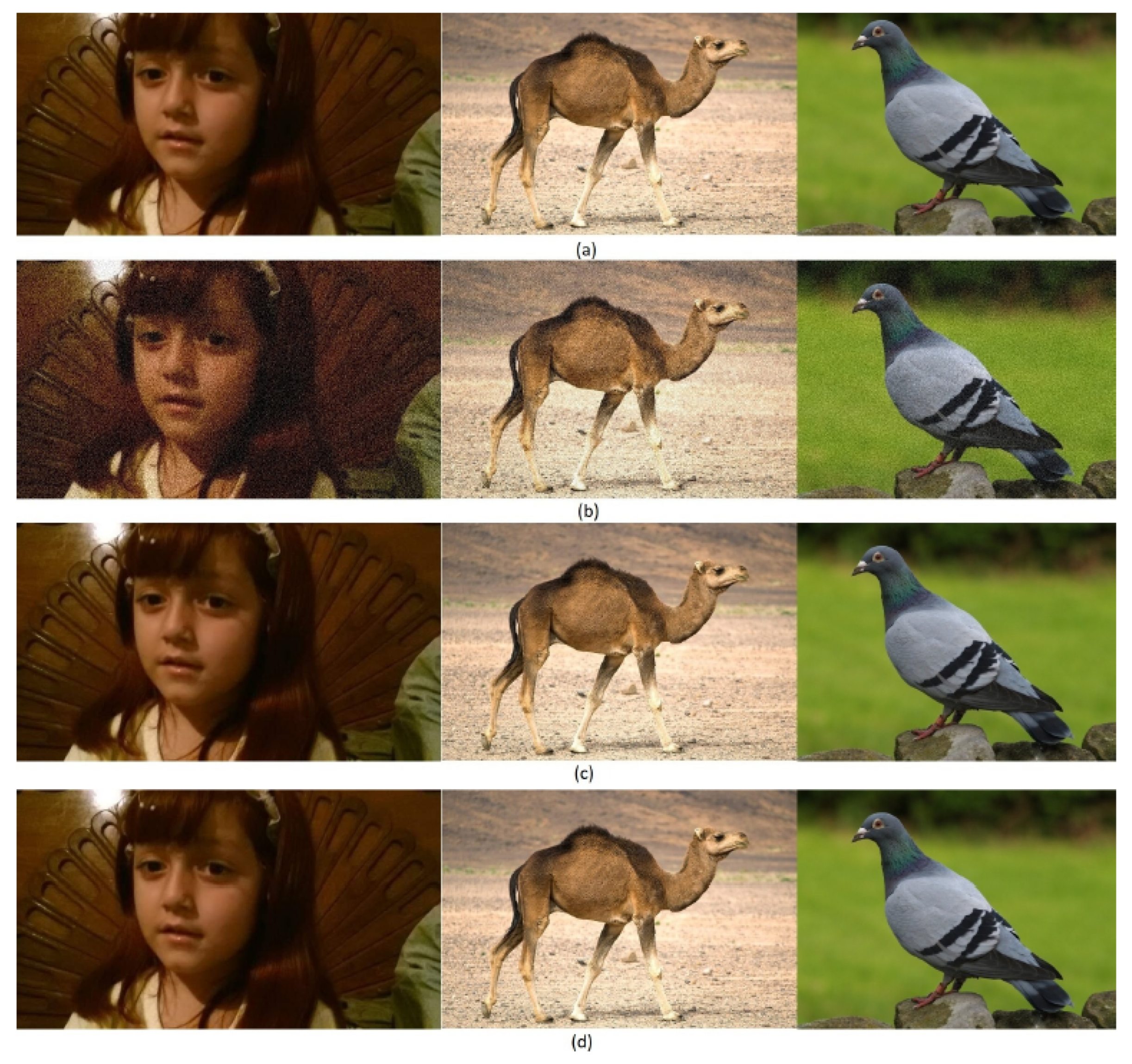
The Figure 1 shows the original image, the noisy image, and the denoised images obtained using the proposed method and other state-of-the-art method (BM3D).

Figure 1. Image comparison: (a) original, (b) noisy, (c) proposed method, and (d) BM3D.

Theoretical Results.

Theorem 3. 

Consider $\mathcal{N}=C\left([a,b]\right)$. Define $d:C\left([a,b]\right)\times C\left([a,b]\right)\to \mathbb{C}$ by

$$d\left(\phi ,\varphi \right)=\underset{t\in [a,b]}{max}\left|\phi (t)-\varphi (t)\right|e^{i\theta },$$

then $\left(\mathcal{N},d\right)$ is a complete C-VSMS with $\theta ={\displaystyle \frac{\pi }{4}}$ and $⋏=1$. Assume that the following conditions hold:

(i) There exists a constant $M>0$ such that

$$\left|k(t,\omega )\right|\le M,$$

for all $(t,\omega )\in [a,b]\times [a,b];$

(ii) The function k is continuous on $[a,b]\times [a,b]$ and $f\in C\left([a,b]\right);$

(iii) There exists a constant $\varpi \in [0,1)$ defined by

$$\varpi =\left|\mu \right|M\left(b-a\right)<1.$$

Then the integral Equation (36) has a unique solution in $C\left([a,b]\right)$.

Proof. 

Define the mapping $\mathfrak{J}:C\left([a,b]\right)\to C\left([a,b]\right)$ by

$$\mathfrak{J}\phi (t)=f(t)+\mu {\int }_a^{b}k(t,\omega )\phi (\omega )d\omega .$$

Consider $\phi ,\varphi \in C\left([a,b]\right).$ Then

$$\begin{array}{ccc}\hfill d(\mathfrak{J}\phi ,\mathfrak{J}\varphi )& =& \underset{t\in [a,b]}{max}\left|\mathfrak{J}\phi (t)-\mathfrak{J}\varphi (t)\right|e^{i\theta }\hfill \\ & =& \left|\mu \right|\underset{t\in [a,b]}{max}\left|{\int }_a^{b}k(t,\omega )\left[\phi (\omega )-\varphi (\omega )\right]d\omega \right|e^{i\theta }\hfill \\ & \le & \left|\mu \right|\underset{t\in [a,b]}{max}{\int }_a^b\left|k(t,\omega )\right|\left|\phi (\omega )-\varphi (\omega )\right|\left|e^{i\theta }\right|d\omega e^{i\theta }\hfill \\ & \le & \left|\mu \right|M\underset{\omega \in [a,b]}{max}\left|\phi (\omega )-\varphi (\omega )\right|e^{i\theta }{\int }_a^{b}d\omega \hfill \\ & =& \left|\mu \right|Md(\phi ,\varphi )\left(b-a\right)\hfill \\ & =& \varpi d(\phi ,\varphi ),\hfill \end{array}$$

where

$$d(\phi ,\varphi )\in \left\{d(\phi ,\varphi ),d(\phi ,\mathfrak{J}\phi ),d(\varphi ,\mathfrak{J}\varphi ),{\displaystyle \frac{d(\phi ,\mathfrak{J}\phi )d(\varphi ,\mathfrak{J}\varphi )}{1+d(\phi ,\varphi )}}\right\}.$$

Hence all the conditions of Corollary 1 are satisfied. Therefore, the Fredholm integral equation admits a unique solution, identical to its unique FP. □

Example 5. 

An integral equation

$$\phi (t)-\mu {\int }_a^{b}k(t,\omega )\phi (\omega )d\omega =f(t)$$

has a unique solution $\phi (t)=t^2-{\displaystyle \frac{3}{2}},$ where $[a,b]=[0,1],$ $f(t)=t^2+{\displaystyle \frac{5}{6}},$ $k(t,\omega )=1$ and $\mu =2$.

Example 6. 

An integral equation

$$\phi (t)-\mu {\int }_a^{b}k(t,\omega )\phi (\omega )d\omega =f(t)$$

has a unique solution $\phi (t)=e^t,$ where $[a,b]=[0,1],$ $f(t)=e^t-{\displaystyle \frac{1}{2}}t,$ $k(t,\omega )=t\omega$ and $\mu ={\displaystyle \frac{1}{2}}$.

7. Conclusions

In conclusion, this study successfully established CFP theorems for both single-valued and multivalued mappings in the framework of C-VSMSs. A novel contraction for single-valued mappings was introduced, and a generalized Hausdorff distance was defined for multivalued mappings, paving the way for new results in FP theory. These theoretical advancements were applied to C-VMSs and SMSs, resulting in the derivation of several FP theorems as direct consequences of our main results. The applicability of these theorems was demonstrated through an illustrative example, showcasing their potential for solving nonlinear problems.

Furthermore, we highlighted the practical relevance of our findings by applying them to Fredholm integral equations of the second kind, a key mathematical tool for modeling real-world phenomena such as image denoising. In this context, the Fredholm integral equation models the relationship between the observed noisy image and the true underlying image, where the kernel function captures the blurring effects introduced by noise. The denoising process, involving the solution of the equation, retrieves the original image, with regularization techniques such as Tikhonov regularization ensuring a stable solution.

Beyond these applications, our results open avenues for algorithmic implementations in numerical analysis and computational mathematics. FP algorithms based on our theorems could be developed to enhance denoising techniques, particularly in scenarios involving iterative regularization methods. Additionally, our findings provide a theoretical foundation for comparing different denoising techniques, such as wavelet-based methods, variational models, and deep-learning-based approaches, through an FP framework. These contributions not only extend the understanding of FP theory but also provide a bridge between abstract mathematical principles and practical computational applications in image processing and beyond.

8. Future Work and Open Problems

This study establishes new CFP theorems in C-VSMSs, providing a foundation for further exploration in both theoretical and applied settings. However, several open questions remain that offer avenues for future research:

Generalization to Other Mathematical Structures.

• Extending the current results to more generalized spaces, such as complex-valued extended supra b-metric spaces, elliptic-valued supra metric spaces, and quaternion-valued supra metric spaces.
• Investigating the existence of FPs under weaker contraction conditions or in hybrid metric structures.
• Exploring cyclic, asymptotic, and quasi-contractive mappings for multivalued mappings.

Establishing FP results in these spaces can extend applications to physics, differential equations, and optimization, while relaxing conditions enhances real-world applicability where strict contractions may not hold.

Applications to Partial and Functional Differential Equations.

While this work applies FP results to integral equations, another promising direction is their application to partial differential equations (PDEs) and functional differential equations:

• Studying the existence and stability of solutions to elliptic and parabolic PDEs using fixed-point techniques.
• Extending the results to delay differential equations, particularly in models involving memory effects or time delays.
• Investigating fractional differential equations where non-local operators arise naturally in physics, finance, and biology.

The adaptation of FP theory to these classes of differential equations could lead to significant theoretical and computational advancements.

Computational Methods and Algorithmic Implementations.

While the current study is theoretical, computational aspects are equally important. Future work could involve

• Developing iterative numerical algorithms to approximate FPs, particularly for solving Fredholm integral equations and nonlinear PDEs.
• Implementing machine learning approaches to optimize FP computations and their applications in image denoising.
• Comparing the efficiency and accuracy of different denoising techniques, such as variational methods, wavelet transforms, and deep-learning-based methods, using a FP framework.
• Exploring parallel computing strategies to improve the convergence speed of FP algorithms in large-scale problems.

Such computational approaches would help validate theoretical findings and provide insights into their real-world applicability.

References

- Frechet, M. Sur quelques points du calcul fonctionnel. Rend. Circ. Mat. Palermo. 1906, 22, 1–72. [Google Scholar] [CrossRef] [Scilit]
- Matthews, S.G. Partial metric topology. Ann. N. Y. Acad. Sci. 1994, 728, 183–197. [Google Scholar] [CrossRef] [Scilit]
- Bakhtin, I.A. The contraction mapping principle in almost metric space. Funct. Anal. 1989, 30, 26–37. [Google Scholar]
- Branciari, A. A fixed point theorem of Banach-Caccioppoli type on a class of generalized metric spaces. Publ. Math. Debrecen. 2000, 57, 31–37. [Google Scholar] [CrossRef] [Scilit]
- Huang, L.G.; Zhang, X. Cone metric spaces and fixed point theorems of contractive mappings. J. Math. Anal. Appl. 2007, 332, 1468–1476. [Google Scholar] [CrossRef] [Scilit]
- Berzig, M. First results in suprametric spaces with applications. Mediterr. J. Math. 2022, 19, 226. [Google Scholar] [CrossRef] [Scilit]
- Berzig, M. Fixed point results in generalized suprametric spaces. Topol. Algebra Its Appl. 2023, 11, 20230105. [Google Scholar] [CrossRef] [Scilit]
- Berzig, M. Nonlinear contraction in b-suprametric spaces. J. Anal. 2024, 32, 2401–2414. [Google Scholar] [CrossRef] [Scilit]
- Berzig, M. Strong b-suprametric spaces and fixed point principles. Complex. Anal. Oper. Theory 2024, 18, 148. [Google Scholar] [CrossRef] [Scilit]
- Antón-Sancho, Á. Fixed points of principal E6-bundles over a compact algebraic curve. Quaest. Math. 2024, 47, 501–513. [Google Scholar] [CrossRef] [Scilit]
- Antón-Sancho, Á. Fixed points of involutions of G-Higgs bundle moduli spaces over a compact Riemann surface with classical complex structure group. Front. Math. 2024, 19, 1025–1039. [Google Scholar] [CrossRef] [Scilit]
- Antón-Sancho, Á. Spin(8,C)-Higgs bundles and the Hitchin integrable system. Mathematics 2024, 12, 3436. [Google Scholar] [CrossRef] [Scilit]
- Azam, A.; Fisher, B.; Khan, M. Common fixed point theorems in complex valued metric spaces. Num. Funct. Anal. Optim. 2011, 32, 243–253. [Google Scholar] [CrossRef] [Scilit]
- Rouzkard, F.; Imdad, M. Some common fixed point theorems on complex valued metric spaces. Comp. Math. Appl. 2012, 64, 1866–1874. [Google Scholar] [CrossRef] [Scilit]
- Hussain, N.; Azam, A.; Ahmad, J.; Arshad, M. Common fixed point results in complex valued metric spaces with application to integral equations. Filomat 2014, 28, 1363–1380. [Google Scholar] [CrossRef] [Scilit]
- Ahmad, J.; Klin-eam, C.; Azam, A. Common fixed points for multivalued mappings in complex-valued metric spaces with applications. Abstr. Appl. Anal. 2013, 2013, 854965. [Google Scholar] [CrossRef] [Scilit]
- Azam, A.; Ahmad, J.; Kumam, P. Common fixed point theorems for multi-valued mappings in complex-valued metric spaces. J. Inequal. Appl. 2013, 2013, 578. [Google Scholar] [CrossRef] [Scilit]
- Panda, S.K.; Vijayakumar, V.; Agarwal, R.P. Complex-valued suprametric spaces, related fixed point results, and their applications to Barnsley Fern fractal generation and mixed Volterra–Fredholm integral equations. Fractal Fract. 2024, 8, 410. [Google Scholar] [CrossRef] [Scilit]
- Sintunavarat, W.; Kumam, P. Generalized common fixed point theorems in complex valued metric spaces and applications. J. Inequal. Appl. 2012, 2012, 84. [Google Scholar] [CrossRef] [Scilit]
- Sitthikul, K.; Saejung, S. Some fixed point theorems in complex valued metric spaces. Fixed Point Theory Appl. 2012, 2012, 189. [Google Scholar] [CrossRef] [Scilit]
- Klin-eam, C.; Suanoom, C. Some common fixed point theorems for generalized contractive type mappings on complex valued metric spaces. Abstr. Appl. Anal. 2013, 2013, 604215. [Google Scholar] [CrossRef] [Scilit]
- Zubair, S.T.; Aphane, M.; Mukheimer, A.; Abdeljawad, T. A fixed point technique for solving boundary value problems in branciari suprametric spaces. Results Nonlinear Anal. 2024, 7, 80–93. [Google Scholar]
- Hanjing, A.; Suantai, S. A fast image restoration algorithm based on a fixed point and optimization method. Mathematics 2020, 8, 378. [Google Scholar] [CrossRef] [Scilit]
- Kim, K.S.; Yun, J.H. Image restoration using a fixed point method for a TVL2 regularization problem. Algorithms 2020, 13, 1. [Google Scholar] [CrossRef] [Scilit]
- Cabello, F.; León, J.; Iano, Y.; Arthur, R. Implementation of a fixed-point 2D Gaussian filter for image processing based on FPGA. Int. J. Recent Technol. Eng. 2015, 23, 23–25. [Google Scholar]
- Mishra, A.; Tripathi, P.K.; Agrawal, A.K.; Joshi, D.R. A contraction mapping method in digital image processing. Int. Recent Technol. Eng. 2019, 8, 193–196. [Google Scholar]
- Kaur, A.; Dong, G. A complete review on image denoising techniques for medical images. Neural Process. Lett. 2023, 55, 7807–7850. [Google Scholar] [CrossRef] [Scilit]
- Peng, C.; Rodi, W.L.; Toksöz, M.N. A Tikhonov regularization method for image reconstruction. Acoust. Imaging. 1994, 1994, 153–164. [Google Scholar]
- Mesgarani, H.; Parmour, P. Application of numerical solution of linear Fredholm integral equation of the first kind for image restoration. Math. Sci. 2023, 17, 371–378. [Google Scholar] [CrossRef] [Scilit]
- Lu, Y.; Shen, L.; Xu, Y. Integral equation models for image restoration: High accuracy methods and fast algorithms. Inverse Problems 2010, 26, 045006. [Google Scholar] [CrossRef] [Scilit]
- Samet, B.; Vetro, C.; Vetro, P. Fixed point theorem for α-ψ contractive type mappings. Nonlinear Anal. 2012, 75, 2154–2165. [Google Scholar] [CrossRef] [Scilit]
- Abbas, M.; Rakocević, V.; Leyew, B.T. Common fixed points of (α-ψ)-generalized rational multivalued contractions in dislocated quasi b-metric spaces and applications. Filomat 2017, 31, 3263–3284. [Google Scholar] [CrossRef] [Scilit]
- Nadler, S.B., Jr. Multi-valued contraction mappings. Pacific J. Math. 1969, 30, 475–478. [Google Scholar] [CrossRef] [Scilit]
- Özger, F.; Ersoy, M.T.; Özger, Z.Ö. Existence of solutions: Investigating Fredholm integral equations via a fixed-point theorem. Axioms 2024, 13, 261. [Google Scholar] [CrossRef] [Scilit]
- Ezquerro, J.A.; Hernández-Verón, M.A. On the application of some fixed-point techniques to Fredholm integral equations of the second kind. J. Fixed Point Theory Appl. 2024, 26, 29. [Google Scholar] [CrossRef] [Scilit]
- Mani, G.; Gnanaprakasam, A.J.; Ege, O.; Fatima, N.; Mlaiki, N. Solution of Fredholm integral equation via common fixed point theorem on bicomplex valued b-metric space. Symmetry 2023, 15, 297. [Google Scholar] [CrossRef] [Scilit]
Disclaimer/Publisher’s Note: The statements, opinions and data contained in all publications are solely those of the individual author(s) and contributor(s) and not of MDPI and/or the editor(s). MDPI and/or the editor(s) disclaim responsibility for any injury to people or property resulting from any ideas, methods, instructions or products referred to in the content. |
© 2025 by the author. Licensee MDPI, Basel, Switzerland. This article is an open access article distributed under the terms and conditions of the Creative Commons Attribution (CC BY) license (https://creativecommons.org/licenses/by/4.0/).