Numerical Approximation for a Stochastic Caputo Fractional Differential Equation with Multiplicative Noise

Abstract

We investigate a numerical method for approximating stochastic Caputo fractional differential equations driven by multiplicative noise. The nonlinear functions f and g are assumed to satisfy the global Lipschitz conditions as well as the linear growth conditions. The noise is approximated by a piecewise constant function, yielding a regularized stochastic fractional differential equation. We prove that the error between the exact solution and the solution of the regularized equation converges in the $L^2((0,T)\times \mathrm{\Omega })$ norm with an order of $O(\Delta t^{\alpha -1/2})$, where $\alpha \in (1/2,1]$ is the order of the Caputo fractional derivative, and $\Delta t$ is the time step size. Numerical experiments are provided to confirm that the simulation results are consistent with the theoretical convergence order.

1. Introduction

Consider the stochastic Caputo fractional differential equation driven by a multiplicative noise, with $\alpha \in (1/2,1]$, written as follows [1]:

$$\left\{\begin{array}{c}{}_0{}^{C}D_t^{\alpha }u\left(t\right)=f(t,u\left(t\right))+g(t,u\left(t\right)){\displaystyle \frac{dW\left(t\right)}{dt}},t\in (0,T],\hfill \\ u\left(0\right)=u_0,\hfill \end{array}\right.$$

(1)

where $u_0\in \mathbb{R}$ is a random variable and $W\left(t\right)$ represents the real-valued Brownian motion, defined on a probability space $(\mathrm{\Omega },\mathcal{F},\mathbb{P})$. Here, ${}_0{}^{C}D_t^{\alpha }v\left(t\right)$ denotes the Caputo fractional derivative, written as follows [2]:

$${}_0{}^{C}D_t^{\alpha }v\left(t\right)={\displaystyle \frac{1}{\mathrm{\Gamma }(1-\alpha )}}{\int }_0^t{(t-\tau )}^{-\alpha }{v}^{\prime }\left(\tau \right)d\tau .$$

(2)

The nonlinear functions $f(t,x)$ and $g(t,x)$ satisfy the global Lipschitz conditions and the linear growth conditions, written as follows:

$$\begin{array}{cc}\hfill & \left|f\right(t,x)-f(t,y\left)\right|\le C|x-y|,\left|g\right(t,x)-g(t,y\left)\right|\le C|x-y|,x,y\in \mathbb{R},\hfill \\ \hfill & \left|f\right(t,x\left)\right|\le C(1+|x\left|\right),\left|g\right(t,x\left)\right|\le C(1+|x\left|\right),x\in \mathbb{R}.\hfill \end{array}$$

By integrating (1) with order $\alpha \in (1/2,1]$, we obtain the following stochastic Volterra integral equation (SVIE):

$$u\left(t\right)=u_0+{\displaystyle \frac{1}{\mathrm{\Gamma }\left(\alpha \right)}}{\int }_0^t{(t-\zeta )}^{\alpha -1}f(\zeta ,u\left(\zeta \right))d\zeta +{\displaystyle \frac{1}{\mathrm{\Gamma }\left(\alpha \right)}}{\int }_0^t{(t-\zeta )}^{\alpha -1}g(\zeta ,u\left(\zeta \right))dW\left(\zeta \right),t\in [0,T].$$

(3)

In this paper, we shall consider the following more general stochastic Volterra integral equations (SVIEs) characterized by a weakly singular kernel of the type, with $\beta \in (1/2,1]$ [1]:

$$u\left(t\right)=u_0+{\displaystyle \frac{1}{\mathrm{\Gamma }\left(\alpha \right)}}{\int }_0^t{(t-\zeta )}^{\alpha -1}f(\zeta ,u\left(\zeta \right))d\zeta +{\displaystyle \frac{1}{\mathrm{\Gamma }\left(\beta \right)}}{\int }_0^t{(t-\zeta )}^{\beta -1}g(\zeta ,u\left(\zeta \right))dW\left(\zeta \right),t\in [0,T].$$

(4)

We remark that when $\alpha =\beta$, the Equation (4) reduces to (3) which have been studied in [3,4].

When the singular kernels ${(t-\zeta )}^{1-\alpha }$ and ${(t-\zeta )}^{1-\beta }$ are replaced by smoother functions, numerical methods for stochastic Volterra integral equations (SVIEs) (4) have been studied in recent years. Tudor and Tudor [5] established strong convergence rates for one-step approximations of SVIEs in the mean-square sense. Wen and Zhang [6] improved the rectangular method for SVIEs, proving first-order convergence. Wang [7] approximated SVIE solutions through related SDEs and proposed two numerical schemes: the stochastic theta method and the splitting method. Xiao et al. [8] developed a split-step collocation method with a convergence order of $1/2$. The work done by Liang et al. [9] showed that the Euler–Maruyama (EM) method can attain superconvergence of order 1 under certain boundary conditions on the diffusion kernel. Recent studies have extended Euler schemes to broader classes, including SVIEs with delays, stochastic Volterra integro-differential equations, and stochastic fractional integro-differential equations; see [10,11,12,13,14] for further developments.

Li et al. [1] analyze stochastic Volterra integral equations with weakly singular kernels, proving existence, uniqueness, and Hölder continuity of solutions. They propose two numerical schemes, the Euler–Maruyama and Milstein methods. Both methods derive strong convergence rates in the $L^p$-norm. Specifically, the Euler–Maruyama scheme converges at rate $min\{1-\alpha ,\beta -1/2\}$, while the Milstein scheme achieves $min\{1-\alpha ,2\beta -1\}$ for $1/2<\alpha \le 1$ and $1/2<\beta \le 1$. These rates differ significantly from those for equations with regular kernels, due to the absence of a standard Itô formula, which is instead handled via Taylor expansions. Kamrani [15] studies stochastic fractional differential equations (SFDEs) with additive noise, written as follows:

$$\left\{\begin{array}{c}{\displaystyle {}_0{}^{C}D_t^{\alpha }u\left(t\right)=f(t,u\left(t\right))+{\int }_0^{t}g(t,s)dW\left(s\right),t\in (0,T],}\hfill \\ u\left(0\right)=u_0,\hfill \end{array}\right.$$

(5)

where $\alpha \in (1/2,1]$. Applying the Galerkin method based on orthogonal polynomials such as Jacobi polynomials, convergence of order 1 is established, supported by numerical experiments demonstrating efficiency. The work [16] considers SFDEs driven by integrated multiplicative noise with Caputo derivatives,

$$\left\{\begin{array}{c}{\displaystyle {}_0{}^{C}D_t^{\alpha }u\left(t\right)=f(t,u\left(t\right))+{\int }_0^{t}g(t,u\left(s\right))dW\left(s\right),t\in (0,T],}\hfill \\ u\left(0\right)=u_0,\hfill \end{array}\right.$$

(6)

approximating the noise with piecewise constant functions and proving an error bound of order $\alpha \in (1/2,1]$ in the $L^2((0,T)\times \mathrm{\Omega })$ norm (see references [17,18,19,20,21]), etc.

In this paper, we propose a new numerical method for solving Equation (4) by approximating the noise using a piecewise constant function, leading to a regularized stochastic Volterra integral equation. We observe that the solution of (6) is significantly more regular than that of (4). As a result, the analysis of the numerical method for solving (4) is more technically involved than for (6).

Let us briefly summarize the main results presented in this paper and highlight its novel contributions.

Consider a partition written as follows:

$$0=t_0<t_1<t_2<\cdots <t_{N-1}<t_N=T,$$

of the interval $[0,T]$, where $\Delta t$ denotes the time step size. To handle the stochastic term, we approximate the white noise ${\displaystyle \frac{dW\left(t\right)}{dt}}$ by the following piecewise constant function ${\displaystyle \frac{d\widehat{W}\left(t\right)}{dt}}$, as introduced in [15], for $t\in [0,t_n],n=1,2,\dots ,N$:

$$\begin{array}{c}\hfill {\displaystyle \frac{d\widehat{W}\left(t\right)}{dt}}=\left\{\begin{array}{cc}{\displaystyle \frac{W\left(t_1\right)-W\left(t_0\right)}{\Delta t}}\approx {\displaystyle \frac{\sqrt{\Delta t}·{\eta }_1}{\Delta t}},\hfill & t\in [t_0,t_1),\hfill \\ {\displaystyle \frac{W\left(t_2\right)-W\left(t_1\right)}{\Delta t}}\approx {\displaystyle \frac{\sqrt{\Delta t}·{\eta }_2}{\Delta t}},\hfill & t\in [t_1,t_2),\hfill \\ ⋮\hfill & ⋮\hfill \\ {\displaystyle \frac{W\left(t_n\right)-W\left(t_{n-1}\right)}{\Delta t}}\approx {\displaystyle \frac{\sqrt{\Delta t}·{\eta }_n}{\Delta t}},\hfill & t\in [t_{n-1},t_n),\hfill \end{array}\right.\end{array}$$

where ${\eta }_i\sim \mathcal{N}(0,1)$, $i=1,2,\dots ,n$ are the independent normally distributed random variables. For simplicity, we can express ${\displaystyle \frac{d\widehat{W}\left(t\right)}{dt}}$ as the following:

$${\displaystyle \frac{d\widehat{W}\left(t\right)}{dt}}=\sum _{i=1}^n{\displaystyle \frac{\sqrt{\Delta t}{\chi }_i\left(t\right){\eta }_i}{\Delta t}}=\sum _{i=1}^n{\displaystyle \frac{{\chi }_i\left(t\right){\eta }_i}{\sqrt{\Delta t}}},$$

where

$${\chi }_i\left(t\right)=\left\{\begin{array}{cc}1,\hfill & t\in [t_{i-1},t_i),\hfill \\ 0,\hfill & \mathrm{otherwise}.\hfill \end{array}\right.$$

We then obtain the following regularized stochastic Volterra integral equation corresponding to (4), with $t=t_n$:

$$\widehat{u}\left(t\right)=u_0+{\int }_0^t{\displaystyle \frac{f(\zeta ,\widehat{u}\left(\zeta \right))}{{(t-\zeta )}^{1-\alpha }}}d\zeta +{\int }_0^t{\displaystyle \frac{g(\zeta ,\widehat{u}\left(\zeta \right))}{{(t-\zeta )}^{1-\beta }}}\left[{\displaystyle \frac{d\widehat{W}\left(\zeta \right)}{d\zeta }}\right]d\zeta ,$$

(7)

which can be equivalently rewritten in the following form, with $t=t_n$:

$$\begin{array}{cc}\hfill \widehat{u}\left(t\right)& =u_0+{\int }_0^t{\displaystyle \frac{f(\zeta ,\widehat{u}\left(\zeta \right))}{{(t-\zeta )}^{1-\alpha }}}d\zeta +\sum _{j=0}^{n-1}{\int }_{t_j}^{t_{j+1}}{\displaystyle \frac{g(\zeta ,\widehat{u}\left(\zeta \right))}{{(t-\zeta )}^{1-\beta }}}\left[{\displaystyle \frac{{\int }_{t_j}^{t_{j+1}}dW\left({\zeta }_1\right)}{\Delta t}}\right]d\zeta \hfill \\ \hfill & =u_0+{\int }_0^t{\displaystyle \frac{f(\zeta ,\widehat{u}\left(\zeta \right))}{{(t-\zeta )}^{1-\alpha }}}d\zeta +\sum _{j=0}^{n-1}{\int }_{t_j}^{t_{j+1}}{\displaystyle \frac{g({\zeta }_1,\widehat{u}\left({\zeta }_1\right))}{{(t_n-{\zeta }_1)}^{1-\beta }}}\left[{\displaystyle \frac{{\int }_{t_j}^{t_{j+1}}dW\left(\zeta \right)}{\Delta t}}\right]d{\zeta }_1\hfill \\ \hfill & =u_0+{\int }_0^t{\displaystyle \frac{f(\zeta ,\widehat{u}\left(\zeta \right))}{{(t-\zeta )}^{1-\alpha }}}d\zeta +\sum _{j=0}^{n-1}{\int }_{t_j}^{t_{j+1}}\left[{\displaystyle \frac{1}{\Delta t}}{\int }_{t_j}^{t_{j+1}}{(t_n-{\zeta }_1)}^{\beta -1}g({\zeta }_1,\widehat{u}\left({\zeta }_1\right))d{\zeta }_1\right]dW\left(\zeta \right).\hfill \end{array}$$

In Theorem 2, we show that in the case of additive noise, the approximation error is of order $O(\Delta t^{\beta -1/2})$ in the $L^2((0,T)\times \mathrm{\Omega })$ norm, where $\beta \in (1/2,1]$. In Theorem 4, we establish that in the case of multiplicative noise, the error also attains the same order $O(\Delta t^{\beta -1/2})$ in the $L^2((0,T)\times \mathrm{\Omega })$ norm.

The main contributions of this paper are summarized as follows:

• A regularized stochastic Volterra integral equation is derived by approximating the noise with a piecewise constant function.
• The stability of the regularized stochastic Volterra integral equation is rigorously analyzed.
• The convergence order of the approximation error is shown to be $O(\Delta t^{\beta -1/2})$ for both additive and multiplicative noise cases, where $\beta \in (1/2,1]$.

The paper is organized as follows: In Section 2, we consider the approximation method for the case of additive noise. In Section 3, we extend the analysis to the case of multiplicative noise. Section 4 presents several numerical simulations to verify the theoretical results.

Throughout this paper, we use $C>0$ to denote a generic deterministic constant that depends on T but is independent of the time step size $\Delta t$. The value of C may vary from line to line.

2. The Additive Noise Case

In this section, we consider the approximation of (4) for the additive noise case. Assume that $g(\zeta ,u\left(\zeta \right))=g_1\left(\zeta \right)$ for $\zeta \in [0,T]$ in (4), where $g_1$ satisfies the Lipschitz condition. We first study the regularity of (4).

The following Grönwall Lemma is used in this paper:

Lemma 1

(Grönwall inequality ([15], Lemma 4.1)). Let $z:{\mathbb{R}}_{+}\to {\mathbb{R}}_{+}$ be a function satisfying, for all $t\in [0,T]$, the inequality, written as follows:

$$z\left(t\right)\le a+K{\int }_0^t{(t-s)}^{\sigma }z\left(s\right)\mathrm{d}s,$$

with constants $a>0$, $K>0$, and $\sigma >-1$. Then, there exists a constant $C=C(\sigma ,K,T)$ such that we obtain the following:

$$z\left(t\right)\le Ca,t\in [0,T].$$

Lemma 2.

Assume that $g(\zeta ,u\left(\zeta \right))=g_1\left(\zeta \right)$ for $\zeta \in [0,T]$ in (4), where $g_1$ satisfies the Lipschitz condition. Let $u\left(t\right)$ be the solution of (4). Then, there exists a constant $C=C\left(T\right)$ such that, with $\alpha \in (1/2,1],\beta \in (1/2,1]$, written as follows:

$$\mathbb{E}|u\left(t_2\right)-u\left(t_1\right){|}^2\le C{(t_2-t_1)}^{min(2\alpha ,2\beta -1)}=C{(t_2-t_1)}^{2\beta -1}.$$

Proof. 

We have obtained the following:

$$\begin{array}{cc}\hfill u\left(t_2\right)-u\left(t_1\right)& =\left[{\int }_0^{t_2}{(t_2-\zeta )}^{\alpha -1}f(\zeta ,u\left(\zeta \right))d\zeta -{\int }_0^{t_1}{(t_1-\zeta )}^{\alpha -1}f(\zeta ,u\left(\zeta \right))d\zeta \right]\hfill \\ \hfill & +\left[{\int }_0^{t_2}{(t_2-\zeta )}^{\beta -1}{g}_1\left(\zeta \right)dW\left(\zeta \right)-{\int }_0^{t_1}{(t_1-\zeta )}^{\beta -1}{g}_1\left(\zeta \right)dW\left(\zeta \right)\right]\hfill \\ \hfill & =I+II.\hfill \end{array}$$

For I, see the proof in [16] (Lemma 2), we obtain the following:

$${\mathbb{E}\left|I\right|}^2\le C{(t_2-t_1)}^{2\alpha }\left(1+{\mathbb{E}\left|u\left(0\right)\right|}^2\right)\le C\Delta t^{2\alpha }.$$

Now we turn to $II$.

$$\begin{array}{cc}\hfill II& ={\int }_0^{t_2}{(t_2-\zeta )}^{\beta -1}{g}_1\left(\zeta \right)dW\left(\zeta \right)-{\int }_0^{t_1}{(t_1-\zeta )}^{\beta -1}{g}_1\left(\zeta \right)dW\left(\zeta \right)\hfill \\ \hfill & =\left[{\int }_{t_1}^{t_2}{(t_2-\zeta )}^{\beta -1}{g}_1\left(\zeta \right)dW\left(\zeta \right)\right]+\left[{\int }_0^{t_1}\left({(t_2-\zeta )}^{\beta -1}-{(t_1-\zeta )}^{\beta -1}\right)g_1\left(\zeta \right)dW\left(\zeta \right)\right]\hfill \\ \hfill & =I{I}_1+I{I}_2.\hfill \end{array}$$

For $I{I}_1$, using the Itô isometry and the boundedness of $g_1$ (since $g_1$ satisfies the Lipschitz condition), we have the following:

$$\mathbb{E}|I{I}_1{|}^2\le C{\int }_{t_1}^{t_2}{(t_2-\zeta )}^{2\beta -2}d\zeta \le C\Delta t^{2\beta -1}.$$

For $I{I}_2$, we obtain, using the Itô isometry and the boundedness of $g_1$, the following:

$$\begin{array}{cc}\hfill \mathbb{E}|I{I}_2{|}^2& =\mathbb{E}{\left|{\int }_0^{t_1}\left({(t_2-\zeta )}^{\beta -1}-{(t_1-\zeta )}^{\beta -1}\right)g_1\left(\zeta \right)dW\left(\zeta \right)\right|}^2\hfill \\ \hfill & \le C{\int }_0^{t_1}{\left({\int }_{t_1}^{t_2}{(x-\zeta )}^{\beta -2}dx\right)}^{2}d\zeta \hfill \\ \hfill & \le C\Delta t{\int }_{t_1}^{t_2}\left[{\int }_0^{t_1}{(x-\zeta )}^{2\beta -4}d\zeta \right]dx\le C\Delta t{\int }_{t_1}^{t_2}{(x-t_1)}^{2\beta -3}dx\le C\Delta t^{2\beta -1}.\hfill \end{array}$$

Hence, we obtain the following:

$$\mathbb{E}|u\left(t_2\right)-u\left(t_1\right){|}^2\le C{(t_2-t_1)}^{2\beta -1},$$

which completes the proof of Lemma 2. □

Theorem 1.

Assume that $g(\zeta ,u\left(\zeta \right))=g_1\left(\zeta \right)$ for $\zeta \in [0,T]$ in (7), where $g_1$ satisfies the Lipschitz condition. Let $\widehat{u}\left(t\right)$ be the solution of (7). There holds the following:

$$\mathbb{E}\left({\int }_0^T|\widehat{u}\left(t\right){|}^{2}dt\right)\le C\left(1+\mathbb{E}|\widehat{u}{\left(0\right)|}^2\right).$$

Proof. 

This proof follows a similar method found in [15], Theorem 4.2. Note that by (7) we obtain the following:

$$\begin{array}{cc}\hfill \mathbb{E}\left[{\int }_0^T{\left|\widehat{u}\left(t\right)\right|}^{2}dt\right]& \le C\mathbb{E}\left[{\int }_0^T{\left|\widehat{u}\left(0\right)\right|}^{2}dt\right]+C\mathbb{E}\left[{\int }_0^T{\left({\int }_0^t{\displaystyle \frac{f(\zeta ,\widehat{u}\left(\zeta \right))}{{(t-\zeta )}^{1-\alpha }}}d\zeta \right)}^{2}dt\right]\hfill \\ \hfill & +C\mathbb{E}\left[{\int }_0^T{\left({\int }_0^t{\displaystyle \frac{g\left(\zeta \right)}{{(t-\zeta )}^{1-\beta }}}d\widehat{W}\left(\zeta \right)\right)}^{2}dt\right]\hfill \\ \hfill & \le I+II+III.\hfill \end{array}$$

For $II$, applying a variable change of $v=t-\zeta$, returns the following:

$$\begin{array}{cc}\hfill II& =C\mathbb{E}{\int }_0^T{\left[{\int }_0^t{v}^{\alpha -1}f(t-v,\widehat{u}(t-v))dv\right]}^{2}dt\hfill \\ & =C\mathbb{E}{\int }_0^T{\left[{\int }_0^T{\chi }_{[0,t]}\left(v\right)v^{\alpha -1}f(t-v,\widehat{u}(t-v))dv\right]}^{2}dt,\hfill \end{array}$$

where ${\chi }_{[0,t]}\left(v\right)$ denotes the characteristic function on $[0,t]$.

Using the following Minkowski integral inequality, with $h\in L^2((a,b)\times (c,d))$,

$$\parallel {\int }_c^{d}h(x,y)dy{\parallel }_{L_x^2(a,b)}\le C{\int }_c^d{\parallel h(x,y)\parallel }_{L_x^2(a,b)}dy=C{\int }_c^d{\left[{\int }_a^b{\left|h(x,y)\right|}^{2}dx\right]}^{1/2}dy,$$

(8)

we arrive at the following:

$$\begin{array}{cc}\hfill II& \le C{\left[{\int }_0^T{\left(\mathbb{E}{\int }_0^T|{\chi }_{[0,t]}\left(v\right)v^{\alpha -1}f(t-v,\widehat{u}(t-v)){|}^{2}dt\right)}^{{\displaystyle \frac{1}{2}}}dv\right]}^2\hfill \\ & =C{\left[{\int }_0^T{v}^{\alpha -1}{\left(\mathbb{E}{\int }_v^T|f(t-v,\widehat{u}(t-v)){|}^{2}dt\right)}^{{\displaystyle \frac{1}{2}}}dv\right]}^2\hfill \\ & =C{\left[{\int }_0^T{v}^{\alpha -1}{\left(\mathbb{E}{\int }_0^{T-v}|f(\zeta ,\widehat{u}\left(\zeta \right)){|}^{2}d\zeta \right)}^{{\displaystyle \frac{1}{2}}}dv\right]}^2\hfill \\ & =C{\left[{\int }_0^T{(T-v)}^{\alpha -1}{\left(\mathbb{E}{\int }_0^v|f(\zeta ,\widehat{u}\left(\zeta \right)){|}^{2}d\zeta \right)}^{{\displaystyle \frac{1}{2}}}dv\right]}^2\hfill \end{array}$$

Using the linear growth assumption for f, we have the following:

$$\begin{array}{cc}\hfill II& \le C{\left[{\int }_0^T{(T-v)}^{\alpha -1}{\left(\mathbb{E}{\int }_0^v(1+|\widehat{u}\left(\zeta \right){|}^2)d\zeta \right)}^{{\displaystyle \frac{1}{2}}}dv\right]}^2\hfill \\ \hfill & =C+C{\left[{\int }_0^T{(T-v)}^{\alpha -1}{\left({\int }_0^v\mathbb{E}{\left|\widehat{u}\left(\zeta \right)\right|}^{2}d\zeta \right)}^{{\displaystyle \frac{1}{2}}}dv\right]}^2.\hfill \end{array}$$

(9)

Now we estimate $III$. Note that, with $t=t_n$, we obtain the following:

$$\begin{array}{cc}\hfill & \mathbb{E}{\left[{\int }_0^t{(t-\zeta )}^{\beta -1}{g}_1\left(\zeta \right)d\widehat{W}\left(\zeta \right)\right]}^2\hfill \\ \hfill & =\mathbb{E}|\sum _{j=0}^{n-1}{\int }_{t_j}^{t_{j+1}}{(t_n-\zeta )}^{\beta -1}{g}_1\left(\zeta \right){\displaystyle \frac{{\int }_{t_j}^{t_{j+1}}dW\left({\zeta }_1\right)}{\Delta t}}d\left(\zeta \right){|}^2\hfill \\ \hfill & =\mathbb{E}|\sum _{j=0}^{n-1}{\int }_{t_j}^{t_{j+1}}\left[{\displaystyle \frac{1}{\Delta t}}{\int }_{t_j}^{t_{j+1}}{(t_n-\zeta )}^{\beta -1}{g}_1\left(\zeta \right)d\zeta \right]dW\left({\zeta }_1\right){|}^2\hfill \\ \hfill & \le C\mathbb{E}\sum _{j=0}^{n-1}{\int }_{t_j}^{t_{j+1}}{\displaystyle \frac{1}{\Delta t^2}}|{\int }_{t_j}^{t_{j+1}}{(t_n-\zeta )}^{\beta -1}{g}_1\left(\zeta \right)d\zeta {|}^{2}d{\zeta }_1.\hfill \end{array}$$

Applying Cauchy–Schwarz inequality, we have the following:

$$\begin{array}{cc}\hfill & \mathbb{E}{\left[{\int }_0^t{(t-\zeta )}^{\beta -1}{g}_1\left(\zeta \right)d\widehat{W}\left(\zeta \right)\right]}^2\hfill \\ \hfill & \le C\mathbb{E}\sum _{j=0}^{n-1}{\int }_{t_j}^{t_{j+1}}{\displaystyle \frac{1}{\Delta t^2}}\Delta t{\int }_{t_j}^{t_{j+1}}{(t_n-\zeta )}^{2\beta -2}{g}_1^2\left(\zeta \right)d\zeta d{\zeta }_1\hfill \\ \hfill & =C\mathbb{E}\sum _{j=0}^{n-1}{\int }_{t_j}^{t_{j+1}}{(t_n-\zeta )}^{2\beta -2}{g}_1^2\left(\zeta \right)d\zeta =C\mathbb{E}{\int }_0^{t_n}{(t_n-\zeta )}^{2\beta -2}{g}_1^2\left(\zeta \right)d\zeta .\hfill \end{array}$$

Hence, we obtain the following:

$$\begin{array}{cc}\hfill III& =\mathbb{E}{\int }_0^T{\left[{\int }_0^t{(t-\zeta )}^{\beta -1}{g}_1\left(\zeta \right)d\widehat{W}\left(\zeta \right)\right]}^{2}dt\hfill \\ \hfill & \le C\mathbb{E}{\int }_0^T\left[{\int }_0^t{(t-\zeta )}^{2\beta -2}{g}_1^2\left(\zeta \right)d\zeta \right]dt=C\mathbb{E}{\int }_0^T\left[{\int }_0^t{v}^{2\beta -2}{g}_1^2(t-v)dv\right]dt\hfill \\ \hfill & =C\mathbb{E}{\int }_0^T\left[{\int }_0^T{\chi }_{[0,t]}\left(v\right)v^{2\beta -2}{g}_1^2(t-v)dv\right]dt\hfill \\ \hfill & =C\mathbb{E}{\int }_0^T\left[{\int }_0^T{\chi }_{[0,t]}\left(v\right)v^{2\beta -2}{g}_1^2(t-v)dt\right]dv\hfill \\ \hfill & =C\mathbb{E}{\int }_0^T{v}^{2\beta -2}\left[{\int }_v^T{g}_1^2(t-v)dt\right]dv=C\mathbb{E}{\int }_0^T{v}^{2\beta -2}\left[{\int }_0^{T-v}{g}_1^2\left(\zeta \right)d\zeta \right]dv\hfill \\ \hfill & =C\mathbb{E}{\int }_0^T{(T-v)}^{2\beta -2}\left[{\int }_0^v{g}_1^2\left(\zeta \right)d\zeta \right]dv,\hfill \end{array}$$

(10)

which implies that, by the bounded assumption of $g_1$, the following is valid:

$$III\le C.$$

Thus, we obtain the following:

$$\mathbb{E}\left[{\int }_0^T{\left|\widehat{u}\left(t\right)\right|}^{2}dt\right]\le C\left[1+\mathbb{E}|\widehat{u}{\left(0\right)|}^2\right]+C\left(1+{\left[{\int }_0^T{(\tilde{t}-v)}^{\alpha -1}{\left(\mathbb{E}{\int }_0^v{\left|\widehat{u}\left(\zeta \right)\right|}^{2}d\zeta \right)}^{{\displaystyle \frac{1}{2}}}dv\right]}^2\right).$$

Denote $u_1:[0,T]\to [0,\infty )$ by the following:

$$u_1\left(v\right)={\left(\mathbb{E}{\int }_0^v{\left|\widehat{u}\left(\zeta \right)\right|}^{2}d\zeta \right)}^{{\displaystyle \frac{1}{2}}}.$$

Then we have the following:

$$u_1\left(T\right)\le C{\left(1+\mathbb{E}|\widehat{u}{\left(0\right)|}^2\right)}^{{\displaystyle \frac{1}{2}}}+C{\int }_0^T{(T-v)}^{\alpha -1}{u}_1\left(v\right)dv.$$

Applying Grönwall Lemma, we have the following:

$$u_1\left(T\right)\le C{\left(1+\mathbb{E}|\widehat{u}{\left(0\right)|}^2\right)}^{{\displaystyle \frac{1}{2}}},$$

and thus we obtain the final result, written as follows:

$$\mathbb{E}\left[{\int }_0^T{\left|\widehat{u}\left(t\right)\right|}^{2}dt\right]\le C\left(1+\mathbb{E}|\widehat{u}{\left(0\right)|}^2\right).$$

The proof of Theorem 1 is complete. □

Theorem 2.

Assume that $g(\zeta ,u\left(\zeta \right))=g_1\left(\zeta \right)$ for $\zeta \in [0,T]$ in (4) and (7), where $g_1$ satisfies the Lipschitz condition. Let $u\left(t\right)$ and $\widehat{u}\left(t\right)$ be the solutions of (4) and (7), respectively. Then, we have the following inequality:

$$\mathbb{E}{\int }_0^T|u\left(t\right)-\widehat{u}\left(t\right){|}^{2}dt\le C{(\Delta t)}^{2\beta -1}.$$

Proof. 

The proof follows arguments similar to those in ([15], Theorem 4.3), which treats a slightly different model (5).

Note that the exact solution $u\left(t\right)$ and the approximate solution $\widehat{u}\left(t\right)$ of the regularized stochastic fractional differential equation take the following forms, with $t=t_n$:

$$\begin{array}{c}\hfill u\left(t\right)=u_0+{\int }_0^t{\displaystyle \frac{f(\zeta ,u(\zeta \left)\right)}{{(t-\zeta )}^{1-\alpha }}}d\zeta +\sum _{j=0}^{n-1}{\int }_{t_j}^{t_{j+1}}\left[{\displaystyle \frac{1}{\Delta t}}{\int }_{t_j}^{t_{j+1}}{(t_n-\zeta )}^{\beta -1}{g}_1\left(\zeta \right)d{\zeta }_1\right]dW\left(\zeta \right).\end{array}$$

$$\begin{array}{c}\hfill \widehat{u}\left(t\right)=u_0+{\int }_0^t{\displaystyle \frac{f(\zeta ,\widehat{u}\left(\zeta \right))}{{(t-\zeta )}^{1-\alpha }}}d\zeta +\sum _{j=0}^{n-1}{\int }_{t_j}^{t_{j+1}}\left[{\displaystyle \frac{1}{\Delta t}}{\int }_{t_j}^{t_{j+1}}{(t_n-{\zeta }_1)}^{\beta -1}{g}_1\left({\zeta }_1\right)d{\zeta }_1\right]dW\left(\zeta \right).\end{array}$$

Denote

$$e\left(t\right)=u\left(t\right)-\widehat{u}\left(t\right),$$

We then have, with $t=t_n$, the following

$$\begin{array}{cc}\hfill e\left(t\right)& ={\int }_0^t{(t-\zeta )}^{\alpha -1}\left[f(\zeta ,u\left(\zeta \right))-f(\zeta ,\widehat{u}\left(\zeta \right))\right]d\zeta \hfill \\ \hfill & +\sum _{j=0}^{n-1}{\int }_{t_j}^{t_{j+1}}\left[{\displaystyle \frac{1}{\Delta t}}{\int }_{t_j}^{t_{j+1}}{(t_n-\zeta )}^{\beta -1}{g}_1\left(\zeta \right)d{\zeta }_1-{\displaystyle \frac{1}{\Delta t}}{\int }_{t_j}^{t_{j+1}}{(t_n-{\zeta }_1)}^{\beta -1}{g}_1\left({\zeta }_1\right)d{\zeta }_1\right]dW\left(\zeta \right).\hfill \end{array}$$

Thus, with $t=t_n$, we obtain the following:

$$\begin{array}{cc}\hfill \mathbb{E}{\int }_0^T{\left|e\left(t\right)\right|}^{2}dt\le & C\mathbb{E}{\int }_0^T|{\int }_0^t{(t-\zeta )}^{\alpha -1}\left[f(\zeta ,u\left(\zeta \right))-f(\zeta ,\widehat{u}\left(\zeta \right)\right]d\zeta {|}^{2}dt\hfill \\ \hfill & +C\mathbb{E}{\int }_0^T\left|\sum _{j=0}^{n-1}{\int }_{t_j}^{t_{j+1}}\right[{\displaystyle \frac{1}{\Delta t}}{\int }_{t_j}^{t_{j+1}}{(t_n-\zeta )}^{\beta -1}{g}_1\left(\zeta \right)d{\zeta }_1\hfill \\ \hfill & -{\displaystyle \frac{1}{\Delta t}}{\int }_{t_j}^{t_{j+1}}{(t_n-{\zeta }_1)}^{\beta -1}{g}_1\left({\zeta }_1\right)d{\zeta }_1]dW\left(\zeta \right){|}^{2}dt\hfill \\ \hfill =& I+II.\hfill \end{array}$$

For I we obtain (see the proof of [16], Theorem 4) the following:

$$\begin{array}{cc}\hfill I& \le C\Delta t^{2\alpha }+C{\left[{\int }_0^T{(T-\nu )}^{\alpha -1}{\left(\mathbb{E}{\int }_0^{\nu }{e}^2\left(\zeta \right)d\zeta \right)}^{{\displaystyle \frac{1}{2}}}d\nu \right]}^2.\hfill \end{array}$$

Now we turn to $II$. Note the following:

$$\begin{array}{cc}\hfill & \mathbb{E}\left|\sum _{j=0}^{n-1}{\int }_{t_j}^{t_{j+1}}\right[{\displaystyle \frac{1}{\Delta t}}{\int }_{t_j}^{t_{j+1}}{(t_n-\zeta )}^{\beta -1}{g}_1\left(\zeta \right)d{\zeta }_1\hfill \\ \hfill & -{\displaystyle \frac{1}{\Delta t}}{\int }_{t_j}^{t_{j+1}}{(t_n-{\zeta }_1)}^{\beta -1}{g}_1\left({\zeta }_1\right)d{\zeta }_1]dW\left(\zeta \right){|}^2\hfill \\ \hfill & \le C\mathbb{E}\sum _{j=0}^{n-1}{\int }_{t_j}^{t_{j+1}}|{\displaystyle \frac{1}{\Delta t}}{\int }_{t_j}^{t_{j+1}}{(t_n-\zeta )}^{\beta -1}{g}_1\left(\zeta \right)d{\zeta }_1\hfill \\ \hfill & -{\displaystyle \frac{1}{\Delta t}}{\int }_{t_j}^{t_{j+1}}{(t_n-{\zeta }_1)}^{\beta -1}{g}_1\left({\zeta }_1\right)d{\zeta }_1{|}^{2}d\zeta \hfill \\ \hfill & \le C\mathbb{E}\sum _{j=0}^{n-1}{\int }_{t_j}^{t_{j+1}}|{\displaystyle \frac{1}{\Delta t}}{\int }_{t_j}^{t_{j+1}}\left[{(t_n-\zeta )}^{\beta -1}-{(t_n-{\zeta }_1)}^{\beta -1}\right]g_1\left(\zeta \right)d{\zeta }_1{|}^{2}d\zeta dt\hfill \\ \hfill & +C\mathbb{E}{\int }_0^T\sum _{j=0}^{n-1}{\int }_{t_j}^{t_{j+1}}|{\displaystyle \frac{1}{\Delta t}}{\int }_{t_j}^{t_{j+1}}{(t_n-{\zeta }_1)}^{\beta -1}\left[g_1\left(\zeta \right)-g_1\left({\zeta }_1\right)\right]d{\zeta }_1{|}^{2}d\zeta \hfill \\ \hfill & =I{I}_1+I{I}_2,\hfill \end{array}$$

which implies the following:

$$II\le C{\int }_0^T(I{I}_1+I{I}_2)dt.$$

For $I{I}_1$, since $g_1$ is bounded, we obtain the following

$$\begin{array}{cc}\hfill I{I}_1& =C\mathbb{E}\sum _{j=0}^{n-1}{\int }_{t_j}^{t_{j+1}}|{\displaystyle \frac{1}{\Delta t}}{\int }_{t_j}^{t_{j+1}}\left[{(t_n-\zeta )}^{\beta -1}-{(t_n-{\zeta }_1)}^{\beta -1}\right]g_1\left(\zeta \right)d{\zeta }_1{|}^{2}d\zeta \hfill \\ \hfill & \le C\sum _{j=0}^{n-1}{\int }_{t_j}^{t_{j+1}}|{\displaystyle \frac{1}{\Delta t}}{\int }_{t_j}^{t_{j+1}}\left[{(t_n-\zeta )}^{\beta -1}-{(t_n-{\zeta }_1)}^{\beta -1}\right]d{\zeta }_1{|}^{2}d\zeta \hfill \\ \hfill & \le C\left[\sum _{j=0}^{n-2}{\int }_{t_j}^{t_{j+1}}\right|{\displaystyle \frac{1}{\Delta t}}{\int }_{t_j}^{t_{j+1}}\left[{(t_n-\zeta )}^{\beta -1}-{(t_n-{\zeta }_1)}^{\beta -1}\right]d{\zeta }_1{|}^{2}d\zeta \hfill \\ \hfill & +{\int }_{t_{n-1}}^{t_n}\left|{\displaystyle \frac{1}{\Delta t}}{\int }_{t_{n-1}}^{t_n}\left[{(t_n-\zeta )}^{\beta -1}-{(t_n-{\zeta }_1)}^{\beta -1}\right]d{\zeta }_1{|}^{2}d\zeta \right]\hfill \\ \hfill & =I{I}_{11}+I{I}_{12}.\hfill \end{array}$$

Now we consider $I{I}_{11}$.

$$I{I}_{11}=C\sum _{j=0}^{n-2}{\int }_{t_j}^{t_{j+1}}|{\displaystyle \frac{1}{\Delta t}}{\int }_{t_j}^{t_{j+1}}\left[{(t_n-\zeta )}^{\beta -1}-{(t_n-{\zeta }_1)}^{\beta -1}\right]d{\zeta }_1{|}^{2}d\zeta .$$

Note the following:

$$\begin{array}{cc}\hfill & |{\displaystyle \frac{1}{\Delta t}}{\int }_{t_j}^{t_{j+1}}\left[{(t_n-\zeta )}^{\beta -1}-{(t_n-{\zeta }_1)}^{\beta -1}\right]d{\zeta }_1{|}^2\le C|{\displaystyle \frac{1}{\Delta t}}{\int }_{t_j}^{t_{j+1}}{\int }_{{\zeta }_1}^{\zeta }{(t_n-\tau )}^{\beta -2}d\tau d{\zeta }_1{|}^2\hfill \\ \hfill & \le C|{\displaystyle \frac{1}{\Delta t}}{\int }_{t_j}^{t_{j+1}}{\int }_{{\zeta }_1}^{t_{j+1}}{(t_n-\tau )}^{\beta -2}d\tau d{\zeta }_1{|}^2=C|{\displaystyle \frac{1}{\Delta t}}{\int }_{t_j}^{t_{j+1}}\left[{\int }_{t_j}^{\tau }{(t_n-\tau )}^{\beta -2}d{\zeta }_1\right]d\tau {|}^2\hfill \\ \hfill & =C|{\displaystyle \frac{1}{\Delta t}}{\int }_{t_j}^{t_{j+1}}{(t_n-\tau )}^{\beta -2}·(\tau -t_j)d\tau {|}^2\le C|{\int }_{t_j}^{t_{j+1}}{(t_n-\tau )}^{\beta -2}d\tau {|}^2.\hfill \end{array}$$

Thus, by the Cauchy–Schwartz Inequality, we obtain the following:

$$\begin{array}{cc}\hfill I{I}_{11}& \le C\sum _{j=0}^{n-2}{\int }_{t_j}^{t_{j+1}}|{\int }_{t_j}^{t_{j+1}}{(t_n-\tau )}^{\beta -2}d\tau {|}^{2}ds\le C\mathbb{E}\sum _{j=0}^{n-2}{\int }_{t_j}^{t_{j+1}}·\left[{\int }_{t_j}^{t_{j+1}}{(t_n-\tau )}^{\overline{2\beta }-4}d\tau \right]\Delta tds\hfill \\ \hfill & =C\Delta t^2\sum _{j=0}^{n-2}{\int }_{t_j}^{t_{j+1}}{(t_n-\tau )}^{\overline{2\beta }-4}d\tau \hfill \\ \hfill & =C\Delta t^2·{\int }_{t_0}^{t_{n-1}}{(t_n-\tau )}^{\overline{2\beta }-4}d\tau \le C(\Delta t^2·\Delta t^{2\beta -3})=C\Delta t^{2\beta -1}.\hfill \end{array}$$

Now for $I{I}_{12}$, if $\zeta <{\zeta }_1$, then we have the following:

$$\begin{array}{cc}\hfill I{I}_{12}& ={\int }_{t_{n-1}}^{t_n}|{\displaystyle \frac{1}{\Delta t}}{\int }_{t_{n-1}}^{t_n}\left[{(t_n-\zeta )}^{\beta -1}-{(t_n-{\zeta }_1)}^{\beta -1}\right]d{\zeta }_1{|}^{2}d\zeta \hfill \\ \hfill & \le C{\int }_{t_{n-1}}^{t_n}|{\displaystyle \frac{1}{\Delta t}}{\int }_{t_{n-1}}^{t_n}{(t_n-\zeta )}^{\beta -1}d{\zeta }_1{|}^{2}d\zeta \hfill \\ \hfill & =C{\int }_{t_{n-1}}^{t_n}|{\displaystyle \frac{1}{\Delta t}}·\Delta t^{\beta }{|}^{2}d\zeta \le C\Delta t^{2\beta -2}·\Delta t=C\Delta t^{2\beta -1}.\hfill \end{array}$$

If $\zeta >{\zeta }_1$, then we obtain the following:

$$\begin{array}{cc}\hfill I{I}_{12}& ={\int }_{t_{n-1}}^{t_n}|{\displaystyle \frac{1}{\Delta t}}{\int }_{t_{n-1}}^{t_n}\left[{(t_n-\zeta )}^{\beta -1}-{(t_n-{\zeta }_1)}^{\beta -1}\right]d{\zeta }_1{|}^{2}d\zeta \hfill \\ \hfill & \le C{\int }_{t_{n-1}}^{t_n}|{\displaystyle \frac{1}{\Delta t}}{\int }_{t_{n-1}}^{t_n}{(t_n-\zeta )}^{\beta -1}d{\zeta }_1{|}^{2}d\zeta =C{\int }_{t_{n-1}}^{t_n}{(t_n-\zeta )}^{2\beta -2}d\zeta \le C\Delta t^{2\beta -1}.\hfill \end{array}$$

Thus for $I{I}_1$ we yield the following:

$$\begin{array}{cc}\hfill I{I}_1& =I{I}_{11}+I{I}_{12}\le C\Delta t^{2\beta -1}.\hfill \end{array}$$

Now we turn to $I{I}_2$. We have, by the Lipschitz condition assumption of $g_1\left(\zeta \right)$, the following:

$$\begin{array}{cc}\hfill I{I}_2& =C\mathbb{E}\sum _{j=0}^{n-1}{\int }_{t_j}^{t_{j+1}}|{\displaystyle \frac{1}{\Delta t}}{\int }_{t_j}^{t_{j+1}}{(t_n-{\zeta }_1)}^{\beta -1}\left[g_1\left(\zeta \right)-g_1\left({\zeta }_1\right)\right]d{\zeta }_1{|}^{2}d\zeta \hfill \\ \hfill & \le C\mathbb{E}\sum _{j=0}^{n-1}{\int }_{t_j}^{t_{j+1}}{\displaystyle \frac{1}{\Delta t}}{\int }_{t_j}^{t_{j+1}}{(t_n-{\zeta }_1)}^{2\beta -2}{\left[g_1\left(\zeta \right)-g_1\left({\zeta }_1\right)\right]}^{2}d{\zeta }_{1}d\zeta \hfill \\ \hfill & \le C\sum _{j=0}^{n-1}{\int }_{t_j}^{t_{j+1}}{\displaystyle \frac{1}{\Delta t}}{\int }_{t_j}^{t_{j+1}}{(t_n-{\zeta }_1)}^{2\beta -2}\Delta t^{2}d{\zeta }_{1}d\zeta \hfill \\ \hfill & \le C\sum _{j=0}^{n-1}{\int }_{t_j}^{t_{j+1}}{(t_n-{\zeta }_1)}^{2\beta -2}\Delta t^{2}d{\zeta }_1\le C\Delta t^2{\int }_0^{t_n}{(t_n-{\zeta }_1)}^{2\beta -2}d{\zeta }_1\le C\Delta t^2.\hfill \end{array}$$

Thus we obtain the following:

$$II\le C{\int }_0^T(I{I}_1+I{I}_2)dt\le C{\int }_0^T(\Delta t^{2\beta -1}+\Delta t^2)dt\le C\Delta t^{2\beta -1}.$$

Therefore we arrive at the following:

$$\begin{array}{cc}\hfill \mathbb{E}\left[{\int }_0^T{\left|e\left(t\right)\right|}^{2}dt\right]\le C\Delta t^{2\alpha }+C\Delta t^{2\beta -1}& +C{\left[{\int }_0^T{(T-v)}^{\alpha -1}{\left(\mathbb{E}{\int }_0^v{\left|e\left(\zeta \right)\right|}^{2}d\zeta \right)}^{{\displaystyle \frac{1}{2}}}dv\right]}^2.\hfill \end{array}$$

Denote $u_2:[0,T]\to [0,\infty )$ by the following

$$u_2\left(v\right)={\left(\mathbb{E}{\int }_0^v{\left|\widehat{u}\left(\zeta \right)\right|}^{2}d\zeta \right)}^{{\displaystyle \frac{1}{2}}}.$$

Then we have the following:

$$u_2\left(T\right)\le C\Delta t^{\alpha }+C\Delta t^{\beta -1/2}+C{\int }_0^T{(T-v)}^{\alpha -1}{u}_2\left(v\right)dv.$$

Applying Grönwall Lemma, we have the following:

$$u_2\left(T\right)\le C\Delta t^{\alpha }+C\Delta t^{\beta -1/2},$$

and thus we obtain the following:

$$\mathbb{E}\left[{\int }_0^T{\left|e\left(t\right)\right|}^{2}dt\right]\le C\Delta t^{min(2\alpha ,2\beta -1)}=C\Delta t^{2\beta -1}.$$

Combining these estimates, we obtain the following:

$$\mathbb{E}{\int }_0^T|u\left(t\right)-\widehat{u}\left(t\right){|}^{2}dt\le C\Delta t^{2\beta -1}.$$

The proof of Theorem 2 is now complete. □

3. The Multiplicative Noise Case

In this section, we consider the approximation of (4) for the multiplicative noise case. We first analyze the stability of the solution to (7).

Theorem 3.

Let $\widehat{u}\left(t\right)$ be the solution of (7). Then we have the following:

$$\mathbb{E}\left({\int }_0^T{\left|\widehat{u}\left(t\right)\right|}^{2}dt\right)\le C\left(1+\mathbb{E}|\widehat{u}{\left(0\right)|}^2\right).$$

Proof. 

This proof follows a similar method as in [15], Theorem 4.2. Note that, by (7), we obtain the following:

$$\begin{array}{cc}\hfill \mathbb{E}\left[{\int }_0^T{\left|\widehat{u}\left(t\right)\right|}^{2}dt\right]& \le C\mathbb{E}\left[{\int }_0^T{\left|\widehat{u}\left(0\right)\right|}^{2}dt\right]+C\mathbb{E}\left[{\int }_0^T{\left({\int }_0^t{\displaystyle \frac{f(\zeta ,\widehat{u}\left(\zeta \right))}{{(t-\zeta )}^{1-\alpha }}}d\zeta \right)}^{2}dt\right]\hfill \\ \hfill & +C\mathbb{E}\left[{\int }_0^T{\left({\int }_0^t{\displaystyle \frac{g(\zeta ,\widehat{u}\left(\zeta \right))}{{(t-\zeta )}^{1-\beta }}}d\widehat{W}\left(\zeta \right)\right)}^{2}dt\right]\hfill \\ \hfill & =I+II+III.\hfill \end{array}$$

Case 1: $g=0$, so $III=0$.

Following the same estimate as in the proof of Theorem 1, we have the following:

$$II\le C\left(1+{\left[{\int }_0^T{(\tilde{t}-v)}^{\alpha -1}{\left(\mathbb{E}{\int }_0^v{\left|\widehat{u}\left(\zeta \right)\right|}^{2}d\zeta \right)}^{{\displaystyle \frac{1}{2}}}dv\right]}^2\right).$$

Thus, we obtain the following:

$$\mathbb{E}\left[{\int }_0^T{\left|\widehat{u}\left(t\right)\right|}^{2}dt\right]\le C\left(1+\mathbb{E}|\widehat{u}{\left(0\right)|}^2\right)+C\left(1+{\left[{\int }_0^T{(T-v)}^{\alpha -1}{\left(\mathbb{E}{\int }_0^v{\left|\widehat{u}\left(\zeta \right)\right|}^{2}d\zeta \right)}^{{\displaystyle \frac{1}{2}}}dv\right]}^2\right).$$

The definition is as follows:

$$u_1\left(t\right)={\left(\mathbb{E}{\int }_0^t{\left|\widehat{u}\left(v\right)\right|}^{2}dv\right)}^{{\displaystyle \frac{1}{2}}}.$$

Hence, we obtain the following:

$$u_1\left(T\right)\le C{\left(1+\mathbb{E}|\widehat{u}{\left(0\right)|}^2\right)}^{{\displaystyle \frac{1}{2}}}+C{\int }_0^T{(T-v)}^{\alpha -1}{u}_1\left(v\right)dv.$$

Applying the Grönwall inequality for fractional integrals, we conclude the following:

$$u_1\left(T\right)\le C{\left(1+\mathbb{E}|\widehat{u}{\left(0\right)|}^2\right)}^{{\displaystyle \frac{1}{2}}},$$

which implies the following:

$$\mathbb{E}\left[{\int }_0^T{\left|\widehat{u}\left(t\right)\right|}^{2}dt\right]\le C\left(1+\mathbb{E}|\widehat{u}{\left(0\right)|}^2\right).$$

Case 2: $f=0$, so $II=0$.

For $III$, following the same argument as in (10), we have the following:

$$\begin{array}{cc}\hfill III& \le C\mathbb{E}{\int }_0^T{(T-\nu )}^{2\beta -2}\left[{\int }_0^{\nu }{\left|g(\zeta ,\widehat{u}\left(\zeta \right))\right|}^{2}d\zeta \right]d\nu \hfill \\ & \le C\mathbb{E}{\int }_0^T{(T-\nu )}^{2\beta -2}\left[{\int }_0^{\nu }\left(1+|g(\zeta ,\widehat{u}\left(\zeta \right)){|}^2\right)d\zeta \right]d\nu \hfill \\ & \le C+C{\int }_0^T{(T-\nu )}^{2\beta -2}\left[{\int }_0^{\nu }\mathbb{E}{\left|\widehat{u}\left(\zeta \right)\right|}^{2}d\zeta \right]d\nu .\hfill \end{array}$$

Therefore, we obtain the following:

$$\mathbb{E}{\int }_0^T{\left|\widehat{u}\left(t\right)\right|}^{2}dt\le C\left(1+\mathbb{E}|\widehat{u}{\left(0\right)|}^2\right)+C{\int }_0^T{(T-\nu )}^{2\beta -2}\left[{\int }_0^{\nu }\mathbb{E}{\left|\widehat{u}\left(\zeta \right)\right|}^{2}d\zeta \right]d\nu .$$

Let the following be valid:

$$u_2\left(\nu \right)={\int }_0^{\nu }\mathbb{E}{\left|\widehat{u}\left(\zeta \right)\right|}^{2}d\zeta .$$

Then we obtain the following:

$$u_2\left(T\right)\le C\left(1+\mathbb{E}|\widehat{u}{\left(0\right)|}^2\right)+C{\int }_0^T{(T-\nu )}^{2\beta -2}{u}_2\left(\nu \right)d\zeta ,$$

By the Grönwall lemma, we obtain the following:

$$\mathbb{E}\left[{\int }_0^T|\widehat{u}\left(t\right){|}^{2}dt\right]\le C\left(1+\mathbb{E}|\widehat{u}{\left(0\right)|}^2\right).$$

Together these estimates complete the proof of Thoerem 3. □

We will now consider the regularity of the solution of (4).

Lemma 3.

Let $u\left(t\right)$ be the solution of (4). Then, we have the following:

$$\mathbb{E}|u\left(t_2\right)-u\left(t_1\right){|}^2\le C{(t_2-t_1)}^{2\beta -1}.$$

Proof. 

We have the following:

$$\begin{array}{cc}\hfill u\left(t_2\right)-u\left(t_1\right)& =\left[{\int }_0^{t_2}{(t_2-\zeta )}^{\alpha -1}f(\zeta ,u\left(\zeta \right))d\zeta -{\int }_0^{t_1}{(t_1-\zeta )}^{\alpha -1}f(\zeta ,u\left(\zeta \right))d\zeta \right]\hfill \\ \hfill & +\left[{\int }_0^{t_2}{(t_2-\zeta )}^{\beta -1}g(\zeta ,u(\zeta \left)\right)dW\left(\zeta \right)-{\int }_0^{t_1}{(t_1-\zeta )}^{\beta -1}g(\zeta ,u(\zeta \left)\right)dW\left(\zeta \right)\right]\hfill \\ \hfill & =I+II.\hfill \end{array}$$

For I, following the proof of [16], Lemma 2, we obtain the following:

$${\mathbb{E}\left|I\right|}^2\le C{(t_2-t_1)}^{2\alpha }\left[1+{\mathbb{E}\left|u\left(0\right)\right|}^2\right]\le C\Delta t^{2\alpha }.$$

Now we turn to $II$.

$$\begin{array}{cc}\hfill II& ={\int }_0^{t_2}{(t_2-\zeta )}^{\beta -1}g(\zeta ,u(\zeta \left)\right)dW\left(\zeta \right)-{\int }_0^{t_1}{(t_1-\zeta )}^{\beta -1}g(\zeta ,u(\zeta \left)\right)dW\left(\zeta \right)\hfill \\ \hfill & \le \left[{\int }_0^{t_2}{(t_2-\zeta )}^{\beta -1}g(\zeta ,u(\zeta \left)\right)dW\left(\zeta \right)-{\int }_0^{t_1}{(t_2-\zeta )}^{\beta -1}g(\zeta ,u(\zeta \left)\right)dW\left(\zeta \right)\right]\hfill \\ \hfill & +\left[{\int }_0^{t_1}{(t_2-\zeta )}^{\beta -1}g(\zeta ,u(\zeta \left)\right)dW\left(\zeta \right)-{\int }_0^{t_1}{(t_1-\zeta )}^{\beta -1}g(\zeta ,u(\zeta \left)\right)dW\left(\zeta \right)\right]\hfill \\ \hfill & =I{I}_1+I{I}_2.\hfill \end{array}$$

For $I{I}_1$, we have the following:

$$\begin{array}{cc}\hfill \mathbb{E}|I{I}_1{|}^2& =\mathbb{E}|{\int }_0^{t_2}{(t_2-\zeta )}^{\beta -1}g(\zeta ,u(\zeta \left)\right)dW\left(\zeta \right)-{\int }_0^{t_1}{(t_2-\zeta )}^{\beta -1}g(\zeta ,u(\zeta \left)\right)dW\left(\zeta \right){|}^2\hfill \\ \hfill & \le \mathbb{E}|{\int }_{t_1}^{t_2}{(t_2-\zeta )}^{\beta -1}g(\zeta ,u(\zeta \left)\right)dW\left(\zeta \right){|}^2.\hfill \end{array}$$

Using the Itô isometry property, we obtain the following:

$$\mathbb{E}|I{I}_1{|}^2\le {\int }_{t_1}^{t_2}|{(t_2-\zeta )}^{\beta -1}{|}^2·\mathbb{E}|g(\zeta ,u(\zeta \left)\right){|}^{2}d\zeta .$$

It is easy to show that ${\mathbb{E}\left|u\left(t\right)\right|}^2$ is uniformally bounded. We then have the following:

$$\begin{array}{cc}\hfill \mathbb{E}|I{I}_1{|}^2& \le C{\int }_{t_1}^{t_2}{(t_2-\zeta )}^{2\beta -2}d\zeta \le C\Delta t^{2\beta -1}.\hfill \end{array}$$

For $I{I}_2$, we obtain the following:

$$\begin{array}{cc}\hfill \mathbb{E}|I{I}_2{|}^2& =\mathbb{E}|{\int }_0^{t_1}{(t_2-\zeta )}^{\beta -1}g(\zeta ,u(\zeta \left)\right)dW\left(\zeta \right)-{\int }_0^{t_1}{(t_1-\zeta )}^{\beta -1}g(\zeta ,u(\zeta \left)\right)dW\left(\zeta \right){|}^2\hfill \\ \hfill & =\mathbb{E}|{\int }_0^{t_1}\left[{(t_2-\zeta )}^{\beta -1}-{(t_1-\zeta )}^{\beta -1}\right]g(\zeta ,u(\zeta \left)\right)dW\left(\zeta \right){|}^2.\hfill \end{array}$$

Applying the Itô isometry property, we yield the following:

$$\begin{array}{cc}\hfill \mathbb{E}|I{I}_2{|}^2& \le C{\int }_0^{t_1}{\left({(t_2-\zeta )}^{\beta -1}-{(t_1-\zeta )}^{\beta -1}\right)}^2\mathbb{E}|g(\zeta ,u(\zeta \left)\right){|}^{2}d\zeta .\hfill \end{array}$$

Noting again the boundedness of ${\mathbb{E}\left|u\left(t\right)\right|}^2$, we arrive at the following:

$$\begin{array}{cc}\hfill \mathbb{E}|I{I}_2{|}^2& \le C{\int }_0^{t_1}{\left({\int }_{t_1}^{t_2}{(x-\zeta )}^{\beta -2}dx\right)}^{2}d\zeta \le C{\int }_0^{t_1}·\Delta t{\int }_{t_1}^{t_2}{(x-\zeta )}^{2(\beta -2)}dxd\zeta \hfill \\ \hfill & =C\Delta t{\int }_{t_1}^{t_2}\left[{\int }_0^{t_1}{(x-\zeta )}^{2\beta -4}d\zeta \right]dx\le C\Delta t·{\int }_{t_1}^{t_2}{(x-t_1)}^{2\beta -3}dx\hfill \\ \hfill & \le C\Delta t^{2\beta -1}.\hfill \end{array}$$

Hence, we obtain the following:

$$E|u\left(t_2\right)-u\left(t_1\right){|}^2\le C{(t_2-t_1)}^{2\beta -1},$$

which completes the proof of Lemma 3. □

Remark 1.

The difference between Lemma 2 and Lemma 3 is as follows: Lemma 2 considers the case for (4) driven by additive noise with $g(\zeta ,u\left(\zeta \right))=g_1\left(\zeta \right)$, whereas Lemma 3 considers the case for (4) driven by multiplicative noise. Both cases yield the same regularity order $O(\Delta t^{\beta -1/2},\beta \in (1/2,1].$

Now, we introduce the main theorem in this section.

Theorem 4.

Let $u\left(t\right)$ and $\widehat{u}\left(t\right)$ be the solutions of (4) and (7), respectively. Then, we have the following:

$$\mathbb{E}{\int }_0^T|u\left(t\right)-\widehat{u}\left(t\right){|}^{2}dt\le C\Delta t^{2\beta -1}.$$

Proof. 

Note that the exact solution $u\left(t\right)$ and the approximate solution $\widehat{u}\left(t\right)$ of the regularized stochastic fractional differential equation take the following forms, with $t=t_n$

$$u\left(t\right)=u_0+{\int }_0^t{\displaystyle \frac{f(\zeta ,u(\zeta \left)\right)}{{(t-\zeta )}^{1-\alpha }}}d\zeta +\sum _{j=0}^{n-1}{\int }_{t_j}^{t_{j+1}}\left[{\displaystyle \frac{1}{\Delta t}}{\int }_{t_j}^{t_{j+1}}{(t_n-\zeta )}^{\beta -1}g(\zeta ,u\left(\zeta \right))d{\zeta }_1\right]dW\left(\zeta \right).$$

$$\widehat{u}\left(t\right)=u_0+{\int }_0^t{\displaystyle \frac{f(\zeta ,\widehat{u}\left(\zeta \right))}{{(t-\zeta )}^{1-\alpha }}}d\zeta +\sum _{j=0}^{n-1}{\int }_{t_j}^{t_{j+1}}\left[{\displaystyle \frac{1}{\Delta t}}{\int }_{t_j}^{t_{j+1}}{(t_n-{\zeta }_1)}^{\beta -1}g({\zeta }_1,\widehat{u}\left({\zeta }_1\right))d{\zeta }_1\right]dW\left(\zeta \right).$$

Denote this as the following:

$$e\left(t\right)=u\left(t\right)-\widehat{u}\left(t\right).$$

Then, $e\left(t\right)$ satisfies the following equation:

$$\begin{array}{cc}\hfill e\left(t\right)=& {\int }_0^t{(t-\zeta )}^{\alpha -1}\left[f(\zeta ,u\left(\zeta \right))-f(\zeta ,\widehat{u}\left(\zeta \right))\right]d\zeta \hfill \\ \hfill & +\sum _{j=0}^{n-1}{\int }_{t_j}^{t_{j+1}}[{\displaystyle \frac{1}{\Delta t}}{\int }_{t_j}^{t_{j+1}}{(t_n-\zeta )}^{\beta -1}g(\zeta ,u\left(\zeta \right))d{\zeta }_1\hfill \\ \hfill & -{\displaystyle \frac{1}{\Delta t}}{\int }_{t_j}^{t_{j+1}}{(t_n-{\zeta }_1)}^{\beta -1}g({\zeta }_1,\widehat{u}\left({\zeta }_1\right))d{\zeta }_1]dW\left(\zeta \right),\hfill \end{array}$$

which implies the following:

$$\begin{array}{cc}\hfill \mathbb{E}{\int }_0^T{\left|e\left(t\right)\right|}^{2}dt\le & C\mathbb{E}{\int }_0^T|{\int }_0^t{(t-\zeta )}^{\alpha -1}\left[f(\zeta ,u\left(\zeta \right))-f(\zeta ,\widehat{u}\left(\zeta \right)\right]d\zeta {|}^{2}dt\hfill \\ \hfill & +C\mathbb{E}{\int }_0^T\left|\sum _{j=0}^{n-1}{\int }_{t_j}^{t_{j+1}}\right[{\displaystyle \frac{1}{\Delta t}}{\int }_{t_j}^{t_{j+1}}{(t_n-\zeta )}^{\beta -1}g(\zeta ,u\left(\zeta \right))d{\zeta }_1\hfill \\ \hfill & -{\displaystyle \frac{1}{\Delta t}}{\int }_{t_j}^{t_{j+1}}{(t_n-{\zeta }_1)}^{\beta -1}g({\zeta }_1,u\left({\zeta }_1\right))d{\zeta }_1]dW\left(\zeta \right){|}^{2}dt\hfill \\ \hfill =& I+II.\hfill \end{array}$$

For I we obtain (see proof of [16], Theorem 4) the following:

$$\begin{array}{cc}\hfill I& \le C\Delta t^{2\alpha }+C{\left[{\int }_0^T{(T-\nu )}^{\alpha -1}{\left(\mathbb{E}{\int }_0^{\nu }{e}^2\left(\zeta \right)d\zeta \right)}^{{\displaystyle \frac{1}{2}}}d\nu \right]}^2.\hfill \end{array}$$

Now, we turn to $II$. Note the the following:

$$\begin{array}{cc}\hfill & \mathbb{E}\left|\sum _{j=0}^{n-1}{\int }_{t_j}^{t_{j+1}}\right[{\displaystyle \frac{1}{\Delta t}}{\int }_{t_j}^{t_{j+1}}{(t_n-\zeta )}^{\beta -1}g(\zeta ,u\left(\zeta \right))d{\zeta }_1\hfill \\ \hfill & -{\displaystyle \frac{1}{\Delta t}}{\int }_{t_j}^{t_{j+1}}{(t_n-{\zeta }_1)}^{\beta -1}g({\zeta }_1,\widehat{u}\left({\zeta }_1\right))d{\zeta }_1]dW\left(\zeta \right){|}^2\hfill \\ \hfill & \le C\mathbb{E}\sum _{j=0}^{n-1}{\int }_{t_j}^{t_{j+1}}|{\displaystyle \frac{1}{\Delta t}}{\int }_{t_j}^{t_{j+1}}{(t_n-\zeta )}^{\beta -1}g(\zeta ,u\left(\zeta \right))d{\zeta }_1\hfill \\ \hfill & -{\displaystyle \frac{1}{\Delta t}}{\int }_{t_j}^{t_{j+1}}{(t_n-{\zeta }_1)}^{\beta -1}g({\zeta }_1,u\left({\zeta }_1\right))d{\zeta }_1{|}^{2}d\zeta \hfill \\ \hfill & \le C\mathbb{E}\sum _{j=0}^{n-1}{\int }_{t_j}^{t_{j+1}}|{\displaystyle \frac{1}{\Delta t}}{\int }_{t_j}^{t_{j+1}}\left[{(t_n-\zeta )}^{\beta -1}-{(t_n-{\zeta }_1)}^{\beta -1}\right]g(\zeta ,u\left(\zeta \right))d{\zeta }_1{|}^{2}d\zeta \hfill \\ \hfill & +C\mathbb{E}\sum _{j=0}^{n-1}{\int }_{t_j}^{t_{j+1}}|{\displaystyle \frac{1}{\Delta t}}{\int }_{t_j}^{t_{j+1}}{(t_n-{\zeta }_1)}^{\beta -1}\left[g(\zeta ,u\left(\zeta \right))-g({\zeta }_1,\widehat{u}\left({\zeta }_1\right))\right]d{\zeta }_1{|}^{2}d\zeta \hfill \\ \hfill & =I{I}_1+I{I}_2,\hfill \end{array}$$

which implies the following:

$$II\le C{\int }_0^T(I{I}_1+I{I}_2)dt.$$

Following the same argument as in the proof of Theorem 2, we have the following:

$$\begin{array}{cc}\hfill I{I}_1& \le C\Delta t^{2\beta -1}.\hfill \end{array}$$

Now we turn to consider $I{I}_2$.

$$\begin{array}{cc}\hfill I{I}_2& =C\mathbb{E}\sum _{j=0}^{n-1}{\int }_{t_j}^{t_{j+1}}|{\displaystyle \frac{1}{\Delta t}}{\int }_{t_j}^{t_{j+1}}{(t_n-{\zeta }_1)}^{\beta -1}\left[g(\zeta ,u\left(\zeta \right))-g({\zeta }_1,\widehat{u}\left({\zeta }_1\right))\right]d{\zeta }_1{|}^{2}d\zeta \hfill \\ \hfill & \le C\mathbb{E}\sum _{j=0}^{n-1}{\int }_{t_j}^{t_{j+1}}|{\displaystyle \frac{1}{\Delta t}}{\int }_{t_j}^{t_{j+1}}{(t_n-{\zeta }_1)}^{\beta -1}\left[g({\zeta }_1,u\left({\zeta }_1\right))-g({\zeta }_1,\widehat{u}\left({\zeta }_1\right))\right]d{\zeta }_1{|}^{2}d\zeta \hfill \\ \hfill & +C\mathbb{E}\sum _{j=0}^{n-1}{\int }_{t_j}^{t_{j+1}}|{\displaystyle \frac{1}{\Delta t}}{\int }_{t_j}^{t_{j+1}}{(t_n-{\zeta }_1)}^{\beta -1}\left[g(\zeta ,u\left(\zeta \right))-g({\zeta }_1,u\left({\zeta }_1\right))\right]d{\zeta }_1{|}^{2}d\zeta \hfill \\ \hfill & =I{I}_2^1+I{I}_2^2.\hfill \end{array}$$

For $I{I}_2^2$, we have, by the Lipschitz assumption of g and Lemma 3, the following:

$$\begin{array}{cc}\hfill I{I}_2^2& =C\mathbb{E}\sum _{j=0}^{n-1}{\int }_{t_j}^{t_{j+1}}|{\displaystyle \frac{1}{\Delta t}}{\int }_{t_j}^{t_{j+1}}{(t_n-{\zeta }_1)}^{\beta -1}\left[g(\zeta ,u\left(\zeta \right))-g({\zeta }_1,u\left({\zeta }_1\right))\right]d{\zeta }_1{|}^{2}d\zeta \hfill \\ \hfill & \le C\mathbb{E}\sum _{j=0}^{n-1}{\int }_{t_j}^{t_{j+1}}\left|{\displaystyle \frac{1}{\Delta t}}{\int }_{t_j}^{t_{j+1}}{(t_n-{\zeta }_1)}^{\beta -1}{\left[g(\zeta ,u\left(\zeta \right))-g({\zeta }_1,u\left({\zeta }_1\right))\right]}^{2}d{\zeta }_1\right|d\zeta \hfill \\ \hfill & \le C\mathbb{E}\sum _{j=0}^{n-1}{\int }_{t_j}^{t_{j+1}}{(t_n-{\zeta }_1)}^{\beta -1}\left[\Delta t^{2\beta -2}\right]d{\zeta }_1\hfill \\ \hfill & \le C\Delta t^{2\beta -1}{\int }_0^{t_n}{(t_n-{\zeta }_1)}^{\beta -1}d{\zeta }_1\le C\Delta t^{2\beta -1}.\hfill \end{array}$$

For $I{I}_2^1$, we have, by the Lipschitz assumption of g, the following:

$$\begin{array}{c}\hfill I{I}_2^1\le C{\int }_0^{t_n}{(t_n-{\zeta }_1)}^{2\beta -2}\mathbb{E}{\left|e\left({\zeta }_1\right)\right|}^{2}d{\zeta }_1.\end{array}$$

(11)

Thus, we obtain, by (10), the following:

$$\begin{array}{cc}\hfill \mathbb{E}\left[{\int }_0^T{\left|e\left(t\right)\right|}^{2}dt\right]& \le C\Delta t^{2\alpha }+C{\left[{\int }_0^T{(T-v)}^{\alpha -1}{\left(\mathbb{E}{\int }_0^v{\left|e\left(\zeta \right)\right|}^{2}d\zeta \right)}^{{\displaystyle \frac{1}{2}}}dv\right]}^2\hfill \\ \hfill & C\Delta t^{2\beta -1}+C{\int }_0^T{(T-v)}^{2\beta -2}\left(\mathbb{E}{\int }_0^v{\left|e\left(\zeta \right)\right|}^{2}d\zeta \right)dv.\hfill \end{array}$$

Case 1. When $g=0$, we have the following:

$$\begin{array}{cc}\hfill \mathbb{E}\left[{\int }_0^T{\left|e\left(t\right)\right|}^{2}dt\right]\le C\Delta t^{2\alpha }& +C{\left[{\int }_0^T{(T-v)}^{\alpha -1}{\left(\mathbb{E}{\int }_0^v{\left|e\left(\zeta \right)\right|}^{2}d\zeta \right)}^{{\displaystyle \frac{1}{2}}}dv.\right]}^2\hfill \end{array}$$

Denote $u_3:[0,T]\to [0,\infty )$ by the following:

$$u_3\left(v\right)={\left(\mathbb{E}{\int }_0^v{\left|\widehat{u}\left(\zeta \right)\right|}^{2}d\zeta \right)}^{{\displaystyle \frac{1}{2}}}.$$

Then we have the following:

$$u_3\left(T\right)\le C\Delta t^{\alpha }+C{\int }_0^T{(T-v)}^{\alpha -1}{u}_3\left(v\right)dv.$$

Applying Grönwall Lemma, we have the following:

$$u_3\left(T\right)\le C\Delta t^{\alpha },$$

and thus we obtain the following:

$$\mathbb{E}\left[{\int }_0^T{\left|e\left(t\right)\right|}^{2}dt\right]\le C\Delta t^{2\alpha }.$$

Case 2. When $f=0$, we have the following:

$$\begin{array}{c}\hfill \mathbb{E}\left[{\int }_0^T{\left|e\left(t\right)\right|}^{2}dt\right]\le C\Delta t^{2\beta -1}+C{\int }_0^T{(T-v)}^{2\beta -2}\left(\mathbb{E}{\int }_0^v{\left|e\left(\zeta \right)\right|}^{2}d\zeta \right)dv.\end{array}$$

(12)

Denote $u_4:[0,T]\to [0,\infty )$ by the following:

$$u_4\left(v\right)=\mathbb{E}{\int }_0^v{\left|\widehat{u}\left(\zeta \right)\right|}^{2}d\zeta .$$

Then we have the following:

$$u_4\left(T\right)\le C\Delta t^{2\beta -1}+C{\int }_0^T{(T-v)}^{2\beta -2}{u}_4\left(v\right)dv.$$

Applying Grönwall Lemma, we have the following:

$$u_4\left(T\right)\le C\Delta t^{2\beta -1},$$

and thus we obtain the following:

$$\mathbb{E}\left[{\int }_0^T{\left|e\left(t\right)\right|}^{2}dt\right]\le C\Delta t^{2\beta -1}.$$

The proof of Theorem 4 is now complete. □

Remark 2.

The difference between Theorem 2 and Theorem 4 is as follows: Theorem 2 considers the convergence order for (4) driven by additive noise with $g(\zeta ,u\left(\zeta \right))=g_1\left(\zeta \right)$, whereas Theorem 4 considers the convergence order for (4) driven by multiplicative noise with $g(\zeta ,u(\zeta \left)\right).$ The additive case yields a convergence order of $O(\Delta t^{\beta -1/2}),\beta \in (1/2,1]$, whereas the multiplicative case achieves a convergence order of $O(\Delta t^{\beta -1/2}),\beta \in (1/2,1]$.

4. Numerical Simulations

Consider the following stochastic fractional differential equation:

$${}_0{}^{C}D_t^{\alpha }u\left(t\right)=f\left(u\left(t\right)\right)+g\left(u\left(t\right)\right){\displaystyle \frac{dW\left(t\right)}{dt}},u\left(0\right)=u_0,$$

where $\alpha \in (1/2,1]$ and $W\left(t\right)$ is a standard Brownian motion.

The equivalent integral form is as follows:

$$u\left(t\right)=u_0+{\displaystyle \frac{1}{\mathrm{\Gamma }\left(\alpha \right)}}{\int }_0^t{(t-s)}^{\alpha -1}f\left(u\left(s\right)\right)ds+{\displaystyle \frac{1}{\mathrm{\Gamma }\left(\alpha \right)}}{\int }_0^t{(t-s)}^{\alpha -1}g\left(u\left(s\right)\right)dW\left(s\right).$$

(13)

Below we shall consider the numerical approximation of the following integral equation:

$$u\left(t\right)=u_0+{\displaystyle \frac{1}{\mathrm{\Gamma }\left(\alpha \right)}}{\int }_0^t{(t-s)}^{\alpha -1}f\left(u\left(s\right)\right)ds+{\displaystyle \frac{1}{\mathrm{\Gamma }\left(\beta \right)}}{\int }_0^t{(t-s)}^{\beta -1}g\left(u\left(s\right)\right)dW\left(s\right),$$

(14)

where the orders satisfy $1/2<\alpha \le 1$ and $1/2<\beta \le 1$ and $W\left(t\right)$ is a standard Brownian motion.

Let $u_m\approx u\left(t_m\right)$ be the approximate solution. We obtain the following:

$$u_m=u_0+{\displaystyle \frac{1}{\mathrm{\Gamma }\left(\alpha \right)}}{\int }_0^{t_m}{(t_m-s)}^{\alpha -1}f\left(u\left(s\right)\right)ds+{\displaystyle \frac{1}{\mathrm{\Gamma }\left(\beta \right)}}{\int }_0^{t_m}{(t_m-s)}^{\beta -1}g\left(u\left(s\right)\right)d\widehat{W}\left(s\right),$$

(15)

where $\widehat{W}\left(s\right)$ is the piecewise constant function approximation of $W\left(s\right)$. In our numerical simulation, we will approximate $f\left(u\right)$ and $g\left(u\right)$ by $f\left(u_k\right)$ and $g\left(u_k\right)$, respectively on the subinterval $[t_k,t_{k+1}]$. This approximation preserves the expected convergence order of $\Delta t^{\beta -1/2}$ since $\beta \in (1/2,1)$. More precisely, we calculate $u_m$ by the following formula:

$$\begin{array}{cc}\hfill u_m& \approx u_0+{\displaystyle \frac{1}{\mathrm{\Gamma }\left(\alpha \right)}}\sum _{k=0}^{m-1}{\int }_{t_k}^{t_{k+1}}{(t_m-s)}^{\alpha -1}f\left(u_k\right)ds+{\displaystyle \frac{1}{\mathrm{\Gamma }\left(\beta \right)}}\sum _{k=0}^{m-1}{\int }_{t_k}^{t_{k+1}}{(t_m-s)}^{\beta -1}g\left(u_k\right)dW\left(s\right)\hfill \\ \hfill & \approx u_0+{\displaystyle \frac{1}{\mathrm{\Gamma }(\alpha +1)}}\sum _{k=0}^{m-1}\left({(t_m-t_k)}^{\alpha }-{(t_m-t_{k+1})}^{\alpha }\right)f\left(u_k\right)\hfill \\ \hfill & +{\displaystyle \frac{1}{\mathrm{\Gamma }\left(\beta \right)}}\sum _{k=0}^{m-1}{(t_m-t_k)}^{\beta -1}g\left(u_k\right)\left(W\left(t_{k+1}\right)-W\left(t_k\right)\right).\hfill \end{array}$$

where $W\left(t_{k+1}\right)-W\left(t_k\right)\sim \sqrt{\Delta t}\mathcal{N}(0,1).$

The algorithm employs numerical integration combined with Monte Carlo simulations to approximate the solution of the Equation (15) and to analyze the associated errors and convergence behavior. We compute approximate solutions using several discretization levels corresponding to step sizes $\Delta t=2^{-5},2^{-6},2^{-7},2^{-8}$. A finer step size of $\Delta t=2^{-12}$, together with 50 Monte Carlo samples, is used to generate a reference solution for comparison.

Step-by-Step Algorithm

• Step 1

Compute $u_1\approx u\left(t_1\right)$:

$$\begin{array}{cc}\hfill u_1& =u_0+{\displaystyle \frac{1}{\mathrm{\Gamma }(\alpha +1)}}\left({(t_1-t_0)}^{\alpha }\right)f\left(u_0\right)+{\displaystyle \frac{1}{\mathrm{\Gamma }\left(\beta \right)}}{(t_1-t_0)}^{\beta -1}g\left(u_0\right)\left(W\left(t_1\right)-W\left(t_0\right)\right).\hfill \end{array}$$

• Step 2

Compute $u_2\approx u\left(t_2\right)$:

$$\begin{array}{cc}\hfill u_2& =u_0+{\displaystyle \frac{1}{\mathrm{\Gamma }(\alpha +1)}}\sum _{k=0}^1\left({(t_2-t_k)}^{\alpha }-{(t_2-t_{k+1})}^{\alpha }\right)f\left(u_k\right)\hfill \\ \hfill & +{\displaystyle \frac{1}{\mathrm{\Gamma }\left(\beta \right)}}\sum _{k=0}^1{(t_2-t_k)}^{\beta -1}g\left(u_k\right)\left(W\left(t_{k+1}\right)-W\left(t_k\right)\right).\hfill \end{array}$$

• Step m

Compute $u_m\approx u\left(t_m\right)$:

$$\begin{array}{cc}\hfill u_m& =u_0+{\displaystyle \frac{1}{\mathrm{\Gamma }(\alpha +1)}}\sum _{k=0}^{m-1}\left({(t_m-t_k)}^{\alpha }-{(t_m-t_{k+1})}^{\alpha }\right)f\left(u_k\right)\hfill \\ \hfill & +{\displaystyle \frac{1}{\mathrm{\Gamma }\left(\beta \right)}}\sum _{k=0}^{m-1}{(t_m-t_k)}^{\beta -1}g\left(u_k\right)\left(W\left(t_{k+1}\right)-W\left(t_k\right)\right).\hfill \end{array}$$

Each step requires storing all previous values $u_0,u_1,\dots ,u_{m-1}$ in order to compute $u_m$.

To analyze convergence, we compute the error at final time $T=1$ and assume a approximate estimate of the following form:

$$\mathrm{error}\left(h\right)=\parallel U^N-u\left(T\right)\parallel \le C{h}^p,p>0.$$

For step sizes $h_i=2^{-i}$, $i=5,6,7,8$, we define the error as follows:

$$\mathrm{error}\left(h_i\right)=\mathbb{E}{\left[\parallel U^{N_i}{-u\left(T\right)\parallel }^2\right]}^{1/2}\approx C{h}_i^p.$$

The experimental order of convergence p is then estimated using the following:

$$p\approx {\displaystyle \frac{{log}_2\left(\frac{\mathrm{error}\left(h_i\right)}{\mathrm{error}\left(h_{i+1}\right)}\right)}{{log}_2\left(\frac{h_i}{h_{i+1}}\right)}}.$$

This procedure allows us to test and compare the accuracy of the numerical method under different configurations of the drift and diffusion terms $f\left(u\right)$ and $g\left(u\right)$ and to assess the rate of convergence numerically.

We derive four distinct EOCs using four step sizes, denoted as $h_i$ for values of $i=4,5,6,7,8$. We then calculate the average of these four EOCs, which can be found in the EOC column of the Table 1, Table 2, Table 3, Table 4, Table 5 and Table 6.

Table 1. Convergence orders for Equation (15) defined by (16) with fixed $\alpha =0.9$ and varying $\beta$.

β	${\mathit{h}}_1=\frac{1}{16}$	${\mathit{h}}_2=\frac{1}{32}$	${\mathit{h}}_3=\frac{1}{64}$	${\mathit{h}}_4=\frac{1}{128}$	${\mathit{h}}_5=\frac{1}{256}$	EOC
0.5	$8.6280\times {10}^{-1}$	$7.6180\times {10}^{-1}$	$6.5860\times {10}^{-1}$	$5.5070\times {10}^{-1}$	$4.5370\times {10}^{-1}$	0.2318
		0.1795	0.2101	0.2581	0.2796
0.6	$2.8520\times {10}^{-1}$	$2.5920\times {10}^{-1}$	$2.2440\times {10}^{-1}$	$1.9750\times {10}^{-1}$	$1.5400\times {10}^{-1}$	0.2221
		0.1376	0.2083	0.1842	0.3584
0.7	$3.1000\times {10}^{-2}$	$2.3000\times {10}^{-2}$	$1.7000\times {10}^{-2}$	$1.3000\times {10}^{-2}$	$1.0000\times {10}^{-2}$	0.4071
		0.4297	0.4353	0.3849	0.3785
0.8	$3.1000\times {10}^{-2}$	$2.3000\times {10}^{-2}$	$1.7000\times {10}^{-2}$	$1.3000\times {10}^{-2}$	$1.0000\times {10}^{-2}$	0.4631
		0.3387	0.4137	0.4840	0.6161
0.9	$6.9000\times {10}^{-3}$	$4.8000\times {10}^{-3}$	$3.4000\times {10}^{-3}$	$2.4000\times {10}^{-3}$	$1.7000\times {10}^{-3}$	0.5057
		0.5261	0.4837	0.5267	0.4863

Table 2. Convergence orders for Equation (15) defined by (17) with fixed $\beta =0.9$ and varying $\alpha$.

α	${\mathit{h}}_1=\frac{1}{16}$	${\mathit{h}}_2=\frac{1}{32}$	${\mathit{h}}_3=\frac{1}{64}$	${\mathit{h}}_4=\frac{1}{128}$	${\mathit{h}}_5=\frac{1}{256}$	EOC
0.5	$6.8000\times {10}^{-3}$	$4.9000\times {10}^{-3}$	$3.6000\times {10}^{-3}$	$2.4000\times {10}^{-3}$	$1.7000\times {10}^{-3}$	0.5070
		0.4599	0.4600	0.5817	0.5264
0.6	$5.8000\times {10}^{-3}$	$4.2000\times {10}^{-3}$	$3.1000\times {10}^{-3}$	$2.3000\times {10}^{-3}$	$1.7000\times {10}^{-3}$	0.4407
		0.4645	0.4331	0.4297	0.4353
0.7	$5.3000\times {10}^{-3}$	$4.1000\times {10}^{-3}$	$2.9000\times {10}^{-3}$	$2.2000\times {10}^{-3}$	$1.5000\times {10}^{-3}$	0.4504
		0.3883	0.5065	0.4067	0.5002
0.8	$6.9000\times {10}^{-3}$	$5.2000\times {10}^{-3}$	$3.7000\times {10}^{-3}$	$2.5000\times {10}^{-3}$	$1.6000\times {10}^{-3}$	0.5364
		0.4073	0.4840	0.5562	0.6982
0.9	$6.9000\times {10}^{-3}$	$4.8000\times {10}^{-3}$	$3.4000\times {10}^{-3}$	$2.4000\times {10}^{-3}$	$1.7000\times {10}^{-3}$	0.5057
		0.5261	0.4837	0.5267	0.4863

Table 3. Convergence orders for Equation (15) defined by (18) with fixed $\alpha =0.9$ and varying $\beta$.

β	${\mathit{h}}_1=\frac{1}{16}$	${\mathit{h}}_2=\frac{1}{32}$	${\mathit{h}}_3=\frac{1}{64}$	${\mathit{h}}_4=\frac{1}{128}$	${\mathit{h}}_5=\frac{1}{256}$	EOC
0.5	$3.8460\times {10}^{-1}$	$3.3930\times {10}^{-1}$	$2.9870\times {10}^{-1}$	$2.4400\times {10}^{-1}$	$2.0380\times {10}^{-1}$	0.2289
		0.1805	0.1839	0.2918	0.2595
0.6	$1.4040\times {10}^{-1}$	$1.2730\times {10}^{-1}$	$1.1040\times {10}^{-1}$	$9.4900\times {10}^{-2}$	$7.5000\times {10}^{-2}$	0.2261
		0.1422	0.2046	0.2191	0.3387
0.7	$4.0800\times {10}^{-2}$	$3.4700\times {10}^{-2}$	$2.6600\times {10}^{-2}$	$2.2200\times {10}^{-2}$	$1.7000\times {10}^{-2}$	0.3161
		0.2349	0.3800	0.2616	0.3879
0.8	$1.5200\times {10}^{-2}$	$1.2000\times {10}^{-2}$	$9.0000\times {10}^{-3}$	$6.5000\times {10}^{-3}$	$4.2000\times {10}^{-3}$	0.4609
		0.3412	0.4108	0.4773	0.6145
0.9	$3.4000\times {10}^{-3}$	$2.6000\times {10}^{-3}$	$1.9000\times {10}^{-3}$	$1.4000\times {10}^{-3}$	$1.1000\times {10}^{-3}$	0.4057
		0.3849	0.4497	0.4397	0.3485

Table 4. Convergence orders for Equation (15) defined by (19) with fixed $\beta =0.9$ and varying $\alpha$.

α	${\mathit{h}}_1=\frac{1}{16}$	${\mathit{h}}_2=\frac{1}{32}$	${\mathit{h}}_3=\frac{1}{64}$	${\mathit{h}}_4=\frac{1}{128}$	${\mathit{h}}_5=\frac{1}{256}$	EOC
0.5	$3.5000\times {10}^{-3}$	$2.5000\times {10}^{-3}$	$1.8000\times {10}^{-3}$	$1.2000\times {10}^{-3}$	$8.0000\times {10}^{-4}$	0.5159
		0.4549	0.4708	0.5870	0.5508
0.6	$2.9000\times {10}^{-3}$	$2.3000\times {10}^{-3}$	$1.7000\times {10}^{-3}$	$1.3000\times {10}^{-3}$	$9.0000\times {10}^{-4}$	0.4399
		0.3594	0.4120	0.3642	0.6240
0.7	$2.7000\times {10}^{-3}$	$2.1000\times {10}^{-3}$	$1.4000\times {10}^{-3}$	$1.1000\times {10}^{-3}$	$8.0000\times {10}^{-4}$	0.4532
		0.3825	0.5169	0.4118	0.5014
0.8	$3.5000\times {10}^{-3}$	$2.6000\times {10}^{-3}$	$1.9000\times {10}^{-3}$	$1.3000\times {10}^{-3}$	$8.0000\times {10}^{-4}$	0.5334
		0.4103	0.4806	0.5528	0.6902
0.9	$3.4000\times {10}^{-3}$	$2.4000\times {10}^{-3}$	$1.7000\times {10}^{-3}$	$1.2000\times {10}^{-3}$	$8.0000\times {10}^{-4}$	0.5041
		0.5105	0.4828	0.5451	0.4781

Table 5. Convergence orders for Equation (15) defined by (20) with fixed $\alpha =0.9$ and varying $\beta$.

β	${\mathit{h}}_1=\frac{1}{16}$	${\mathit{h}}_2=\frac{1}{32}$	${\mathit{h}}_3=\frac{1}{64}$	${\mathit{h}}_4=\frac{1}{128}$	${\mathit{h}}_5=\frac{1}{256}$	EOC
0.5	$6.4550\times {10}^{-1}$	$6.6620\times {10}^{-1}$	$5.4180\times {10}^{-1}$	$4.5860\times {10}^{-1}$	$4.0360\times {10}^{-1}$	0.1694
		-0.0456	0.2981	0.2407	0.1844
0.6	$2.4460\times {10}^{-1}$	$2.2800\times {10}^{-1}$	$2.0620\times {10}^{-1}$	$1.8760\times {10}^{-1}$	$1.4620\times {10}^{-1}$	0.1856
		0.1011	0.1453	0.1363	0.3595
0.7	$7.2300\times {10}^{-2}$	$6.0700\times {10}^{-2}$	$4.7500\times {10}^{-2}$	$4.0800\times {10}^{-2}$	$3.1300\times {10}^{-2}$	0.3023
		0.2512	0.3545	0.2204	0.3831
0.8	$2.4600\times {10}^{-2}$	$1.8900\times {10}^{-2}$	$1.4100\times {10}^{-2}$	$1.0400\times {10}^{-2}$	$7.9000\times {10}^{-3}$	0.4114
		0.3806	0.4183	0.4392	0.4075
0.9	$5.8000\times {10}^{-3}$	$4.2000\times {10}^{-3}$	$3.3000\times {10}^{-3}$	$2.5000\times {10}^{-3}$	$1.7000\times {10}^{-3}$	0.4455
		0.4645	0.3332	0.4453	0.5389

Table 6. Convergence orders for Equation (15) defined by (21) with fixed $\beta =0.9$ and varying $\alpha$.

α	${\mathit{h}}_1=\frac{1}{16}$	${\mathit{h}}_2=\frac{1}{32}$	${\mathit{h}}_3=\frac{1}{64}$	${\mathit{h}}_4=\frac{1}{128}$	${\mathit{h}}_5=\frac{1}{256}$	EOC
0.5	$6.9000\times {10}^{-3}$	$5.5000\times {10}^{-3}$	$3.7000\times {10}^{-3}$	$2.5000\times {10}^{-3}$	$2.0000\times {10}^{-3}$	0.4561
		0.3406	0.5716	0.5685	0.3436
0.6	$5.6000\times {10}^{-3}$	$4.1000\times {10}^{-3}$	$3.1000\times {10}^{-3}$	$2.3000\times {10}^{-3}$	$1.9000\times {10}^{-3}$	0.3891
		0.4500	0.4010	0.4297	0.2756
0.7	$5.0000\times {10}^{-3}$	$3.8000\times {10}^{-3}$	$2.8000\times {10}^{-3}$	$2.1000\times {10}^{-3}$	$1.5000\times {10}^{-3}$	0.4340
		0.4050	0.4309	0.3818	0.5184
0.8	$5.7000\times {10}^{-3}$	$4.1000\times {10}^{-3}$	$3.0000\times {10}^{-3}$	$2.1000\times {10}^{-3}$	$1.5000\times {10}^{-3}$	0.4816
		0.4708	0.4737	0.4882	0.4938
0.9	$5.8000\times {10}^{-3}$	$4.2000\times {10}^{-3}$	$3.3000\times {10}^{-3}$	$2.5000\times {10}^{-3}$	$1.7000\times {10}^{-3}$	0.4455
		0.4645	0.3332	0.4453	0.5389

We consider the following choices of functions $f(t,u(t\left)\right)$ and $g(t,u(t\left)\right)$:

$$\begin{array}{cc}\hfill & f(t,u(t\left)\right)=-u\left(t\right),g(t,u(t\left)\right)=1,\alpha =0.9,\hfill \end{array}$$

(16)

$$\begin{array}{cc}\hfill & f(t,u(t\left)\right)=-u\left(t\right),g(t,u(t\left)\right)=1,\beta =0.9,\hfill \end{array}$$

(17)

$$\begin{array}{cc}\hfill & f(t,u\left(t\right))={\displaystyle \frac{u\left(t\right)}{1+{\left(u\left(t\right)\right)}^2}},g(t,u\left(t\right))={\displaystyle \frac{u\left(t\right)}{1+{\left(u\left(t\right)\right)}^2}},\alpha =0.9,\hfill \end{array}$$

(18)

$$\begin{array}{cc}\hfill & f(t,u\left(t\right))={\displaystyle \frac{u\left(t\right)}{1+{\left(u\left(t\right)\right)}^2}},g(t,u\left(t\right))={\displaystyle \frac{u\left(t\right)}{1+{\left(u\left(t\right)\right)}^2}},\beta =0.9,\hfill \end{array}$$

(19)

$$\begin{array}{cc}\hfill & f(t,u(t\left)\right)=sin\left(u\right(t\left)\right),g(t,u(t\left)\right)=sin\left(u\right(t\left)\right),\alpha =0.9,\hfill \end{array}$$

(20)

$$\begin{array}{cc}\hfill & f(t,u(t\left)\right)=sin\left(u\right(t\left)\right),g(t,u(t\left)\right)=sin\left(u\right(t\left)\right),\beta =0.9.\hfill \end{array}$$

(21)

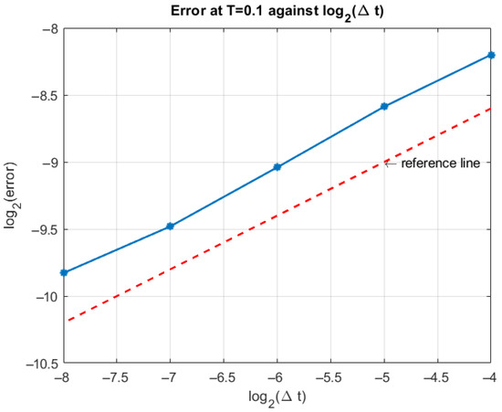
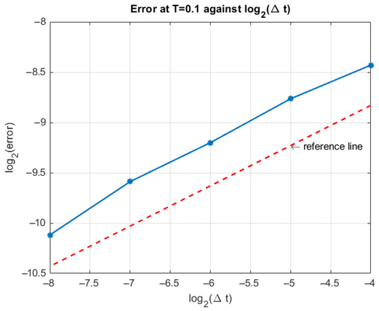
We observe that the convergence orders are approximately $O(\Delta t^{\beta -1/2})$ for different values of $\alpha \in (1/2,1]$ and $\beta \in (1/2,1]$. This is consistent with the theoretical order $O(\Delta t^{2\beta -1})$ for both additive and multiplicative noises.

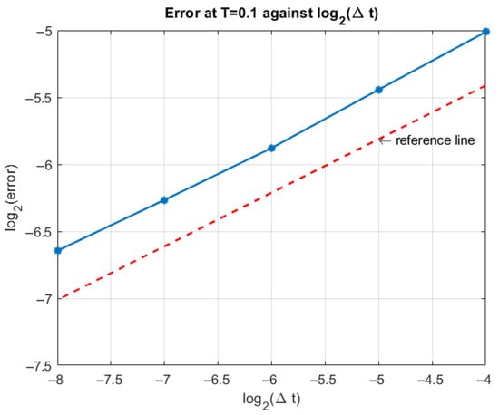
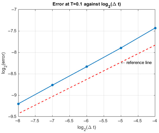
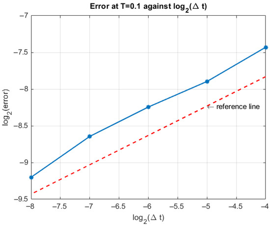
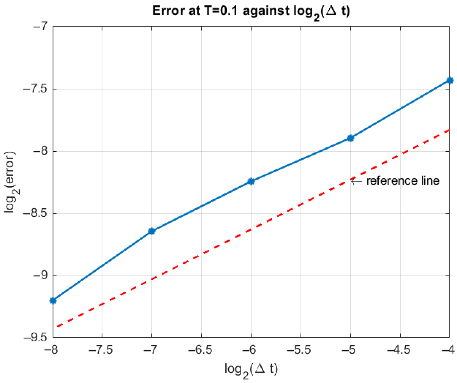
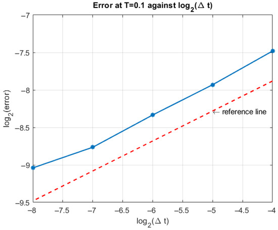
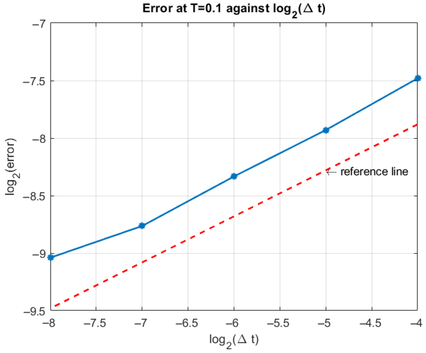
Figure 1 and Figure 2 illustrate the order of convergence plotted against varying values of $\alpha$, using data from Table 1 and Table 2, which correspond to additive noise cases. In both figures, the theoretical convergence order $\beta -0.5=0.3$ (for $\beta =0.8$) and $\beta -0.5=0.4$ (for $\beta =0.9$), respectively, are marked as reference lines.

Figure 1. Convergence order for Equation (15) defined by (16) with $\alpha =0.9$ and $\beta =0.8$.

Figure 2. Convergence order for Equation (15) defined by (17) with $\alpha =0.6$ and $\beta =0.9$.

Figure 3, Figure 4, Figure 5 and Figure 6 present similar plots based on Table 3, Table 4, Table 5 and Table 6, which correspond to multiplicative noise cases. Here, the theoretical convergence order $\beta -0.5=0.4$ (with $\beta =0.9$) is again used as a reference line. The convergence orders observed in all figures show a parallel line to the reference line of $\beta -0.5$ for both additive noise and multiplicative noise cases.

Figure 3. Convergence order for Equation (15) defined by (18) with $\alpha =0.9$ and $\beta =0.9$.

Figure 4. Convergence order for Equation (15) defined by (19) with $\alpha =0.6$ and $\beta =0.9$.

Figure 5. Convergence order for Equation (15) defined by (20) with $\alpha =0.9$ and $\beta =0.9$.

Figure 6. Convergence order for Equation (15) defined by (21) with $\alpha =0.6$ and $\beta =0.9$.

5. Conclusions

This paper considered the numerical approximation of stochastic Caputo fractional differential equations with multiplicative noise. The approach involved approximating the noise using a piecewise constant function, leading to a regularized stochastic fractional differential equation. We established the regularity of the solution and analyzed the convergence order of the proposed numerical scheme. Numerical simulations were performed using the Monte Carlo method to estimate the error and evaluate the experimental order of convergence (EOC). The results demonstrated that, for both additive and multiplicative noise cases, the convergence order was approximately $O(\Delta t^{\beta -1/2})$, with most EOC values closely matching the theoretical rate $\beta -1/2$, where $\beta \in (1/2,1]$ characterizes the singularity in the stochastic integral of the corresponding stochastic Volterra integral equation. This suggests that the type of noise (additive or multiplicative) and the fractional order $\alpha \in (1/2,1]$ do not significantly influence the convergence rate of the proposed method.

References

- Li, M.; Huang, C.; Hu, Y. Numerical methods for stochastic Volterra integral equations with weakly singular kernels. IMA J. Numer. Anal. 2022, 42, 2656–2683. [Google Scholar] [CrossRef] [Scilit]
- Diethelm, K. The Analysis of Fractional Differential Equations; Lecture Notes in Mathematics; Springer: Berlin/Heidelberg, Germany, 2010. [Google Scholar]
- Kloeden, P.E.; Platen, E. Numerical Solution of Stochastic Differential Equations; Applications of Mathematics (New York); Springer: Berlin/Heidelberg, Germany, 1992; Volume 23. [Google Scholar]
- Milstein, G.N.; Tretyakov, M.V. Stochastic Numerics for Mathematical Physics; Scientific Computation; Springer: Berlin/Heidelberg, Germany, 2004. [Google Scholar]
- Tudor, C.; Tudor, M. Approximation schemes for Itô–Volterra stochastic equations. Bol. Soc. Mat. Mex. 1995, 1, 73–85. [Google Scholar]
- Wen, C.H.; Zhang, T.S. Improved rectangular method on stochastic Volterra equations. J. Comput. Appl. Math. 2011, 235, 2492–2501. [Google Scholar] [CrossRef] [Scilit]
- Wang, Y. Approximate representations of solutions to SVIEs, and an application to numerical analysis. J. Math. Anal. Appl. 2017, 449, 642–659. [Google Scholar] [CrossRef] [Scilit]
- Xiao, Y.; Shi, J.N.; Yang, Z.W. Split-step collocation methods for stochastic Volterra integral equations. J. Integral Equ. Appl. 2018, 30, 197–218. [Google Scholar] [CrossRef] [Scilit]
- Liang, H.; Yang, Z.; Gao, J. Strong superconvergence of the Euler–Maruyama method for linear stochastic Volterra integral equations. J. Comput. Appl. Math. 2017, 317, 447–457. [Google Scholar] [CrossRef] [Scilit]
- Dai, X.; Bu, W.; Xiao, A. Well-posedness and EM approximations for non-Lipschitz stochastic fractional integro-differential equations. J. Comput. Appl. Math. 2019, 356, 377–390. [Google Scholar] [CrossRef] [Scilit]
- Gao, J.; Liang, H.; Ma, S. Strong convergence of the semi-implicit Euler method for nonlinear stochastic Volterra integral equations with constant delay. Appl. Math. Comput. 2019, 348, 385–398. [Google Scholar] [CrossRef] [Scilit]
- Yang, H.; Yang, Z.; Ma, S. Theoretical and numerical analysis for Volterra integro-differential equations with Itô integral under polynomially growth conditions. Appl. Math. Comput. 2019, 360, 70–82. [Google Scholar] [CrossRef] [Scilit]
- Zhang, W. Theoretical and numerical analysis of a class of stochastic Volterra integro-differential equations with non-globally Lipschitz continuous coefficients. Appl. Numer. Math. 2020, 147, 254–276. [Google Scholar] [CrossRef] [Scilit]
- Zhang, W.; Liang, H.; Gao, J. Theoretical and numerical analysis of the Euler–Maruyama method for generalized stochastic Volterra integro-differential equations. J. Comput. Appl. Math. 2020, 365, 17. [Google Scholar] [CrossRef] [Scilit]
- Kamrani, M. Numerical solution of stochastic fractional differential equations. Numer. Algorithms 2015, 68, 81–93. [Google Scholar] [CrossRef] [Scilit]
- Hoult, J.; Yan, Y. Numerical approximation for a stochastic fractional differential equation driven by integrated multiplicative noise. Mathematics 2024, 3, 265. [Google Scholar] [CrossRef] [Scilit]
- Mohammadi, F.; Ciancio, A. Wavelet-based numerical method for solving fractional integro-differential equation with a weakly singular kernel. Wavelet Linear Algebra 2017, 4, 53–73. [Google Scholar]
- Zhang, X. Euler schemes and large deviations for stochastic Volterra equations with singular kernels. J. Differ. Equ. 2008, 244, 2226–2250. [Google Scholar] [CrossRef] [Scilit]
- Asadzade, J.A.; Mahmudov, N.I. Euler-Maruyama approximation for stochastic fractional neutral integro-differential equations with weakly singular kernel. Phys. Scr. 2024, 99, 075281. [Google Scholar] [CrossRef] [Scilit]
- Anh, P.T.; Doan, T.S.; Huong, P.T. A variation of constant formula for Caputo fractional stochastic differential equations. Statist. Probab. Lett. 2019, 145, 351–358. [Google Scholar] [CrossRef] [Scilit]
- Son, D.T.; Huong, P.T.; Kloeden, P.E.; Tuan, H.T. Asymptotic separation between solutions of Caputo fractional stochastic differential equations. Stoch. Anal. Appl. 2018, 36, 654–664. [Google Scholar] [CrossRef] [Scilit]
Disclaimer/Publisher’s Note: The statements, opinions and data contained in all publications are solely those of the individual author(s) and contributor(s) and not of MDPI and/or the editor(s). MDPI and/or the editor(s) disclaim responsibility for any injury to people or property resulting from any ideas, methods, instructions or products referred to in the content. |
© 2025 by the authors. Licensee MDPI, Basel, Switzerland. This article is an open access article distributed under the terms and conditions of the Creative Commons Attribution (CC BY) license (https://creativecommons.org/licenses/by/4.0/).