A Simple Model for Targeting Industrial Investments with Subsidies and Taxes

Abstract

We consider an investor, whose capital is divided into an industrial investment $x_t$ and cash $y_t$, and satisfy a nonlinear deterministic dynamical system. The investor fixes fractions of capital to be invested, withdrawn, and consumed, and also the production factor parameter. The government fixes a subsidy fraction for industrial investments and a tax fraction for the capital outflow. We study a Stackelberg game, corresponding to the asymptotically stable equilibrium $(x^{\ast },y^{\ast })$ of the mentioned dynamical system. In this game, the government (the leader) uses subsidies to make incentives for the investor (the follower) to maintain the desired level of $x^{\ast }$, and uses taxes to achieve this with the minimal cost. The investor’s aim is to maximize the difference between the consumption and the price of the production factor at equilibrium. We present an explicit analytical solution of the specified Stackelberg game. Based on this solution, we introduce the notion of a fair industrial investment level, which is costless for the government, and show that it can produce realistic results using a case study of water production in Lahore.

1. Introduction

In this paper, we introduce and study a simple model for targeting industrial investments with subsidies and taxes. In this model, there are two players: a government, and an investor, who at the same time is the owner of an industrial enterprise (e.g., a farm). The aim of the government is to make incentives for the investor to maintain a specified level of industrial investments. The government cost is the difference between the subsidies on industrial investments and the taxes on the capital outflow from production assets. The aim of the follower is to maximize the difference between the consumption and the price of the production factor (e.g., the labor). The amount of this factor is related to the size of the enterprise.

The described problem can be related to the “targeted economic development” approach [1,2,3,4]. Within this approach, which may be opposed to “economic freedom”, policymakers can use different instruments to “promote the development of particular firms and industries” [4]. We focus on government targeting policies, assuming that there are two instruments, subsidies and taxes, and on mathematical modeling within the Stackelberg game paradigm. Thus, we regard the government as a leader, and the investor as a follower.

There are various targets that can be the aim of a government. By using subsidies and taxes, it can make incentives for adoption of a new technology [5], renewable energy generation and transmission [6], bioelectricity generation [7], product recovery and environmental performance [8], green technology adoption, green production and product development [9,10,11], new drug R&D [12], R&D investment [13], etc. The problem of targeting a monopoly at a desired output level was considered in [14]. The case of agricultural industry was considered in [15]. We also mention a recent survey concerning circular economy systems [16]. In general, the role of subsidies and taxes is important for sustainable development [17,18]. Moreover, the impact of different forms of incentives on the modern economy is so essential that some authoritative economists argue that it is necessary to tame them [19].

There are various possibilities for formalizing the targeting of financial investments problem. We assume that the investor’s capital is divided into an industrial investment $x_t$ and cash $y_t$, and satisfy a nonlinear deterministic dynamical system. The non-linearity concerns the dynamics of $x_t$ and is related to the production function of the enterprise. Furthermore, we assume that the investor fixes fractions of capital to be invested, withdrawn, and consumed. The reason for this assumption is that such fixed fraction strategies appear to be optimal in simplified financial problems concerning investment and consumption [20,21]. Constant rebalancing strategies are also used as benchmarks in the theory of online portfolio selection [22]. Similarly, we assume that the government fixes a subsidy fraction for industrial investments and a tax fraction for the capital outflow. This is a basic form of subsidy/tax strategy [23]. The special feature of our model is the utilization of the Cobb–Douglas production function for modeling the dynamics of $x_t$. This function contains a parameter L (the production factor), selected by the investor by paying the price p per unit of L.

Assuming non-zero consumption, we prove that the mentioned dynamical system has a unique globally asymptotically stable equilibrium $(x^{\ast },y^{\ast })$: Theorem 1. The main part of this paper is devoted to the study of a Stackelberg game, corresponding to $(x^{\ast },y^{\ast })$. In this game, the government (the leader) uses subsidies to make incentives for the investor (the follower) to maintain the desired level $\underline{x}$ of $x^{\ast }$, and uses taxes to achieve this with the minimal cost. The investor’s aim is to maximize the difference between the consumption and the price of the production factor at the equilibrium. The precise formulation of this problem is given in Section 2.

In Section 3 and Section 4, we find optimal investor reactions for fixed subsidy and tax fractions. These reactions are qualitatively different in the two cases where the taxes can be conventionally called large and small, respectively. Using these results, in Section 5, we find the solution to the government optimization problem. It appears that there are three basic cases, depending on the specified level of the desired amount of industrial investment. (1) For small values of $\underline{x}$, subsidies are not required and the government obtains a positive revenue due to the taxation. There are no industrial investments in this case. (2) For middle values of $\underline{x}$, positive subsidies and taxes coexist. (3) For large values of $\underline{x}$, it is optimal to use pure subsidies without taxes. The investor revenue is increasing in $\underline{x}$ in all three cases. Our findings are summarized in Theorems 2 and 3.

Based on the obtained solutions, we introduce the notions of basic and fair industrial investment levels. The basic level is optimal for the government if it does not want to achieve a higher target. The levels below the basic one are not Pareto optimal: they are less favorable for both players. The fair industrial investment level induces neither a cost nor revenue for the government. It plays a key role in Section 6, where we apply our results to the analysis of water production in Lahore, considered in [24], and show that the fair industrial investment level can produce realistic results.

2. Problem Formulation

Consider an investor whose capital is divided into an industrial investment $x_t$ and cash $y_t$. We propose the following model for the dynamics of these components:

$$\begin{array}{cc}\hfill x_{t+1}& =A{L}^{\mu }{((1-\beta )x_t+(1+\delta )\alpha y_t)}^{\nu },\hfill \end{array}$$

(1)

$$\begin{array}{cc}\hfill y_{t+1}& =(1-\alpha -c)y_t+(1-\sigma )\beta x_t,\hfill \end{array}$$

(2)

$$\begin{array}{cc}\hfill & x_0={\overline{x}}_0,y_0={\overline{y}}_0.\hfill \end{array}$$

(3)

Here,

$$(\alpha ,\beta ,c)\in {[0,1]}^3,\alpha +c\le 1,L\ge 0,$$

(4)

are the parameters selected by the investor: $\alpha$ is the fraction of cash, intended for industrial investments, $\beta$ is the withdrawn fraction of industrial investments, c is the fraction of consumed capital, and L is the production factor, which we will call “labor” for simplicity. The parameters

$$\delta \ge 0,\sigma \in [0,1]$$

(5)

are selected by the government: $\delta$ is the fraction of industrial investments paid to the investor as a subsidy, and $\sigma$ is the fraction of withdrawn industrial capital paid by the investor to the government due to the taxation. Finally, the positive constants A, $\mu$, and $\nu$ are the parameters of the Cobb–Douglas production function

$$\Phi (L,Z)=A{L}^{\mu }{Z}^{\nu }.$$

Our standing assumption is

$$\mu +\nu <1,$$

which corresponds to the decreasing returns to scale [25]. Note that we use the Cobb–Douglas production function in a non-traditional way: to model the dynamics of the industrial capital.

To obtain a more intuitive view of the model (1)–(3) consider the case where there are no investments and capital outflow: $\alpha =\beta =0$. Then, the industrial capital $x_t$ will tend to the equilibrium $\tilde{x}$, determined by the positive solution equation

$$\check{x}=A{L}^{\mu }{\check{x}}^{\nu },$$

irrespective of $x_0>0$. The value $\check{x}$ depends on the amount of labor L and the parameters A, $\mu$, and $\nu$ of the model. In fact, when $\check{x}$ is invested, there is no gain or loss (the capital does not change). If, for instance, the investor selects a larger value of $x_0$, then he will suffer a loss. This may correspond to buying a large amount of raw materials, which cannot be fully processed by the enterprise.

Furthermore, we assume that the aim of the government is to ensure the target value $\underline{x}$ of industrial investments. For small values of $\underline{x}$, it may be possible to achieve this only with taxes, determined by $\sigma$. Otherwise, subsidies, determined by $\delta$, are also necessary. It is not clear a priori if it is worth using taxes and subsidies simultaneously (but we will show that usually this is the case). In fact, the situation is more complex, since we will also allow the investor, whose aim is to maximize consumption, to select the amount of labor L at a price p per unit.

The precise problem formulation is based on the asymptotic stability property of the system (1)–(3). First rewrite this using the shorthand notation: $z_t=(x_t,y_t)$,

$$z_{t+1}=F(z_t),z_0={\overline{z}}_0.$$

(6)

We say that an equilibrium $z^{\ast }\in {\mathbb{R}}_{+}^2:=\{z\in {\mathbb{R}}^2:z\ge 0\}$ of (6):

$$z^{\ast }=F(z^{\ast })$$

is globally asymptotically stable in ${\mathbb{R}}_{+}^2\backslash \{0\}$, if ${lim}_{t\to \infty }{z}_t=z^{\ast }$ for any initial condition $z_0\in {\mathbb{R}}_{+}^2\backslash \{0\}$. By this definition, there can be no more than 1 globally asymptotically stable equilibriums. Note also that the case $z^{\ast }=0$ is allowed by this definition.

The mapping $F:{\mathbb{R}}_{+}^2\to {\mathbb{R}}_{+}^2$ is monotone with regards to the natural partial order of ${\mathbb{R}}^2$, generated by ${\mathbb{R}}_{+}^2$:

$$F(z)\le F(z^{\prime }),\mathrm{if}z\le z^{\prime }.$$

Moreover, this mapping F is subhomogeneous [26]:

$$F(\lambda z)\le \lambda F(z),z\in {\mathbb{R}}_{+}^2,\lambda \ge 1.$$

Using these two properties, it is not difficult to prove the following result.

Theorem 1.

Assume that $c>0$ and the conditions (4) and (5) are satisfied. Then, there exists a (unique) globally asymptotically stable equilibrium $z^{\ast }=(x^{\ast },y^{\ast })$ of (1) and (2),

$$\begin{array}{cc}\hfill x^{\ast }& =A^{1/(1-\nu )}{L}^{\mu /(1-\nu )}{\left(1-\beta +(1+\delta )(1-\sigma )\frac{\alpha \beta }{\alpha +c}\right)}^{\nu /(1-\nu )},\hfill \end{array}$$

(7)

$$\begin{array}{cc}\hfill y^{\ast }& =\frac{(1-\sigma )\beta }{\alpha +c}{x}^{\ast }\hfill \end{array}$$

(8)

in ${\mathbb{R}}_{+}^2\backslash \{0\}$.

Proof. 

Solving the equation $z=F(z)$, we can easily conclude that there are two equilibrium points in ${\mathbb{R}}_{+}^2$: the origin $(0,0)$ and $z^{\ast }=(x^{\ast },y^{\ast })$, defined by (7) and (8). Assume that

$$\sigma <1,1-\beta +\alpha >0,L>0.$$

(9)

Then, the components $x^{\ast }$, $y^{\ast }$ are strictly positive. Hence, for any $z_0\in {\mathbb{R}}_{+}^2$, there exists $\lambda \ge 1$ such that $z_0\le \lambda z^{\ast }$. As was mentioned, the mapping F is monotone and subhomogeneous, and it is easy to see that its powers $F^t$ inherit these properties. Thus,

$$z_t=F^t(z_0)\le F^t(\lambda z^{\ast })\le \lambda F^t(z^{\ast })=\lambda z^{\ast }.$$

In particular, the sequence $z_t$ is bounded. Consider any convergent subsequence $z_{t_k}$ of $z_t$. If $z_{t_k}\to z$, then $z_{t_k+1}=F(z_{t_k})$ converges to $F(z)$. Hence, $z\in {\mathbb{R}}_{+}^2$ is an equilibrium. It remains to been shown that $z\ne 0$. Indeed, if this case z coincides with $z^{\ast }$, and if any convergent subsequence of $z_t$ converges to $z^{\ast }$, then $z_t$ itself converges to $z^{\ast }$.

Assume first that $\beta <1$ and consider the one-dimensional sequence

$${\tilde{x}}_{t+1}=A{L}^{\mu }{((1-\beta ){\tilde{x}}_t)}^{\nu },{\tilde{x}}_0=x_0>0.$$

If ${\tilde{x}}_t\le x_t$, then

$${\tilde{x}}_{t+1}\le A{L}^{\mu }{((1-\beta )x_t+(1+\delta )\alpha y_t)}^{\nu }=x_{t+1}.$$

Thus, ${\tilde{x}}_t\le x_t$ for all t. Furthermore,

$$\begin{array}{cc}\hfill {\tilde{x}}_{t+1}& =A{L}^{\mu }{(1-\beta )}^{\nu }{\tilde{x}}_t^{\nu }={\left(A{L}^{\mu }{(1-\beta )}^{\nu }\right)}^{1+\nu }{\tilde{x}}_{t-1}^{{\nu }^2}\hfill \\ \hfill & ={\left(A{L}^{\mu }{(1-\beta )}^{\nu }\right)}^{1+\nu +\cdots +{\nu }^t}{\tilde{x}}_0^{{\nu }^{t+1}}\to {\left(A{L}^{\mu }{(1-\beta )}^{\nu }\right)}^{1/(1-\nu )}>0\hfill \end{array}$$

as $t\to \infty$. Thus, ${lim}_{k\to \infty }{x}_{t_k}\ge {lim}_{k\to \infty }{\tilde{x}}_{t_k}>0$.

Now, let $\beta =1$. Then, $\alpha >0$, $x_{t+1}=A{L}^{\mu }{(1+\delta )}^{\nu }{\alpha }^{\nu }{y}_t^{\nu }$,

$$y_{t+1}=(1-\alpha -c)y_t+(1-\sigma )A{L}^{\mu }{(1+\delta )}^{\nu }{\alpha }^{\nu }{y}_{t-1}^{\nu },t\ge 2.$$

Consider the one-dimensional sequence

$${\tilde{y}}_{t+2}=C{\tilde{y}}_t^{\nu },{\tilde{y}}_0=y_0$$

with $C=A{L}^{\mu }(1-\sigma ){(1+\delta )}^{\nu }{\alpha }^{\nu }$. If ${\tilde{y}}_t\le y_t$, then

$${\tilde{y}}_{t+2}\le (1-\alpha -c)y_{t+1}+C{\tilde{y}}_t^{\nu }\le y_{t+2}.$$

Thus, ${\tilde{y}}_t\le y_t$ for all even indexes: $t=2n$, $n\in {\mathbb{Z}}_{+}$. Since,

$${\tilde{y}}_{2n}=C{\tilde{y}}_{2n-2}^{\nu }=C^{1+\nu }{\tilde{y}}_{2n-2·2}^{{\nu }^2}=C^{1+\nu +\cdots +{\nu }^{n-1}}{\tilde{y}}_0^{{\nu }^n}\to C^{1/(1-\nu )}>0$$

as $n\to \infty$, it follows that if $y_{t_k}\to 0$, then we can assume that the indexes $t_k$ are odd. If also $x_{t_k}\to 0$, then from (2) it follows that $y_{t_k+1}\to 0$. But this is a contradiction, since the indexes $t_k+1$ are even in this case. This finishes the proof under the assumption (9).

If any of the conditions (9) are violated, then from (1) and (2) it follows quite easily that $z_t\to z^{\ast }$, $t\to \infty$.  □

The optimization problems of the agents are formulated within the framework of the Stackelberg games. We assume that the government (the leader) selects $\delta ,\sigma$, the investor (the follower) selects $\alpha ,\beta ,c,L$, and the system (1)–(3) generates the equilibrium (7) and (8). For this equilibrium, the follower computes the revenue

$$c{y}^{\ast }-pL,$$

(10)

and the leader computes the cost

$$\delta \alpha y^{\ast }-\sigma \beta x^{\ast }.$$

(11)

Here, (10) is the difference between the follower consumption and the total cost of labor at the equilibrium, and (11) is the difference between the amount of subsidies and taxes. In the following, we will use the names “leader” and “follower” instead of “government” and “investor”.

According to the protocol of the Stackelberg game, for a given $\delta ,\sigma$ the follower finds $\widehat{\alpha }$, $\widehat{\beta }$, $\widehat{c}$, $\widehat{L}$, which maximize (10) under the constraints (4). These values are substituted in (11) and the leader finds optimal ${\delta }^{\ast }$, ${\sigma }^{\ast }$ by minimizing (11) over the parameters (5) under an additional constraint

$$x^{\ast }\ge \underline{x},$$

(12)

reflecting the main goal of the leader: to ensure the required level $\underline{x}$ of industrial investments.

The case $c=0$ corresponds to zero consumption, and is not interesting for us. So, we will assume that the condition $c>0$ of Theorem 1 is satisfied. Put

$$\gamma =\alpha /c,\rho =(1+\delta )(1-\sigma ).$$

It is natural to call $\gamma$ the investment-to-consumption ratio. From (7) and (8) we obtain

$$\begin{array}{cc}\hfill x^{\ast }& =A^{1/(1-\nu )}{L}^{\mu /(1-\nu )}{\left(1-\beta +\rho \frac{\gamma \beta }{1+\gamma }\right)}^{\nu /(1-\nu )}.\hfill \end{array}$$

$$c{y}^{\ast }=\frac{(1-\sigma )\beta }{1+\gamma }{x}^{\ast },$$

(13)

and the optimization problem (4) and (10) of the follower takes the form

$$\begin{array}{cc}\hfill \underset{\gamma ,\beta ,L}{maximize}& f(\gamma ,\beta ,L)=\frac{(1-\sigma )\beta }{1+\gamma }{x}^{\ast }-pL\hfill \end{array}$$

$$\begin{array}{c}=\frac{(1-\sigma )\beta }{1+\gamma }{A}^{1/(1-\nu )}{L}^{\mu /(1-\nu )}{\left(1-\left(1-\rho \frac{\gamma }{1+\gamma }\right)\beta \right)}^{\nu /(1-\nu )}-pL,\hfill \end{array}$$

(14)

$$\begin{array}{cc}\hfill \mathrm{subject}\mathrm{to}& \gamma \in [0,\infty ),\beta \in [0,1],L\in [0,\infty ).\hfill \end{array}$$

(15)

Note, that the follower’s actions will only determine the product of the capital level $y^{\ast }$ and the consumption fraction c, see (13), and not $y^{\ast }$ and c individually.

Similarly,

$$\alpha y^{\ast }=\gamma c{y}^{\ast }=\frac{(1-\sigma )\beta \gamma }{1+\gamma }{x}^{\ast }$$

(16)

and the leader problem (5) and (10), (12) can be rewritten as

$$\begin{array}{cc}\hfill \underset{\delta ,\sigma }{minimize}& g(\delta ,\sigma )=\left[(1-\sigma )\delta \frac{\gamma }{1+\gamma }-\sigma \right]\beta x^{\ast },\hfill \end{array}$$

(17)

$$\begin{array}{cc}\hfill \mathrm{subject}\mathrm{to}& x^{\ast }\ge \underline{x},\delta \in [0,\infty ),\sigma \in [0,1].\hfill \end{array}$$

(18)

We hide the dependence of f on the parameters of the leader $\delta ,\sigma$, and the dependence of g on the parameters $\gamma$, $\beta$, L of the follower. We repeat that, according to the protocol of the Stackelberg game, the leader looks for the parameters ${\delta }^{\ast }$, ${\sigma }^{\ast }$, solving (17) and (18), where the parameters $\gamma$, $\beta$, L are substituted by the optimal reactions $\widehat{\gamma }(\delta ,\sigma )$, $\widehat{\beta }(\delta ,\sigma )$, $\widehat{L}(\delta ,\sigma )$ of the follower, obtained from (14) and (15).

Although the described Stackelberg game looks cumbersome, we were able to find its explicit solution. The optimal behavior of the agents is described in Theorems 2 and 3. For the follower problem (14) and (15), it appears that the parameter $\rho$ plays a key role and its critical value is 1. For brevity, we can say that the taxes (for the capital outflow) are large if $\rho \le 1$, and small if $\rho >1$. The analysis of this problem is performed in Section 3 and Section 4. For the leader problem, a key role is played by the level $\underline{x}$. This problem is considered in Section 5.

3. Follower’s Problem in the Case of Large Taxes

In this section, we assume that $\rho =(1+\delta )(1-\sigma )\le 1$. To solve (14) and (15) we sequentially consider three one-dimensional optimization problems:

$$\begin{array}{cc}\hfill \underset{\beta \in [0,1]}{maximize}& f(\gamma ,\beta ,L),\hfill \end{array}$$

(19)

$$\begin{array}{cc}\hfill \underset{\gamma \ge 0}{maximize}& f(\gamma ,\widehat{\beta },L),\hfill \end{array}$$

(20)

$$\begin{array}{cc}\hfill \underset{L\ge 0}{maximize}& f(\widehat{\gamma },\widehat{\beta },L),\hfill \end{array}$$

(21)

where $\widehat{\beta }$ is the solution of (19), and $\widehat{\gamma }$ is the solution of (20). Note that $\widehat{\beta }$ can depend on $(\gamma ,L)$, and $\widehat{\gamma }$ can depend on $\widehat{\beta },L$. Certainly, the solution $(\widehat{\beta },\widehat{\gamma },\widehat{L})$ obtained in this sequential manner coincides with the optimal solution of (14) and (15). Note that we do not explicitly show the dependence on the parameters $\delta ,\sigma$.

To solve (19), consider the logarithm of the objective function and the related optimization problem

$$\underset{\beta \in [0,1]}{maximize}\phi (\beta )=ln\beta +\frac{\nu }{1-\nu }ln\left(1-\left(1-\rho \frac{\gamma }{1+\gamma }\right)\beta \right).$$

Solving the equation ${\phi }^{\prime }(\beta )=0$, we conclude that, being extended to $(0,\infty )$, the concave function $\phi$ attains its maximum at

$$\overline{\beta }=\frac{1-\nu }{1-\rho \gamma /(1+\gamma )}.$$

If $\overline{\beta }\le 1$, then $\widehat{\beta }=\overline{\beta }$. Otherwise, $\widehat{\beta }=1$:

$$\widehat{\beta }=\left\{\begin{array}{cc}{\displaystyle \frac{1-\nu }{1-\rho \gamma /(1+\gamma )},}\hfill & {\displaystyle \frac{\gamma }{1+\gamma }\le \frac{\nu }{\rho },}\hfill \\ 1,\hfill & \mathrm{otherwise}.\hfill \end{array}\right.$$

(22)

Note that the second case appears only if $\nu /\rho <1$.

The objective function (20) takes the form

$$f(\gamma ,\widehat{\beta },L)=\left\{\begin{array}{cc}{f}_1(\gamma ,L),\hfill & {\displaystyle \frac{\gamma }{1+\gamma }\le \frac{\nu }{\rho },}\hfill \\ f_2(\gamma ,L),\hfill & \mathrm{otherwise}.\hfill \end{array}\right.$$

(23)

$$\begin{array}{cc}\hfill f_1(\gamma ,L)& {\displaystyle =\frac{(1-\sigma )(1-\nu )}{1+(1-\rho )\gamma }{A}^{1/(1-\nu )}{L}^{\mu /(1-\nu )}{\nu }^{\nu /(1-\nu )}-pL,}\hfill \end{array}$$

(24)

$$\begin{array}{cc}\hfill f_2(\gamma ,L)& {\displaystyle =(1-\sigma )A^{1/(1-\nu )}{L}^{\mu /(1-\nu )}{\rho }^{\nu /(1-\nu )}\frac{{\gamma }^{\nu /(1-\nu )}}{{(1+\gamma )}^{1/(1-\nu )}}-pL.}\hfill \end{array}$$

(25)

The function (24) attains its maximum at $\gamma =0$. If $\rho =1$, then any other value of $\gamma$ is also optimal, but we will assume that the follower still picks $\gamma =0$, since this is the most natural choice: do not invest if the investment does not increase the objective function.

Assuming that $\nu /\rho <1$ and maximizing (25) over $[0,\infty )$, we obtain the solution $\overline{\gamma }$, satisfying the equation $\overline{\gamma }/(1+\overline{\gamma })=\nu$. But due to the constraint

$$\frac{\gamma }{1+\gamma }\ge \frac{\nu }{\rho }\ge \nu ,$$

we conclude that the maximum is attained at the solution of the equation

$$\frac{\gamma }{1+\gamma }=\frac{\nu }{\rho }.$$

Hence, if $\nu /\rho \ge 1$, then $\widehat{\gamma }=0$. Otherwise, to solve the problem (20), we need to compare the expressions

$$\begin{array}{cc}\hfill f_1(0,L)& =(1-\sigma )(1-\nu )A^{1/(1-\nu )}{L}^{\mu /(1-\nu )}{\nu }^{\nu /(1-\nu )}-pL,\hfill \\ \hfill f_2\left(\frac{\nu /\rho }{1-\nu /\rho },L\right)& =(1-\sigma )A^{1/(1-\nu )}{L}^{\mu /(1-\nu )}{\rho }^{\nu /(1-\nu )}{\left(\frac{\nu }{\rho }\right)}^{\nu /(1-\nu )}(1-\nu /\rho )-pL\hfill \\ \hfill & =(1-\sigma )(1-\nu /\rho )A^{1/(1-\nu )}{L}^{\mu /(1-\nu )}{\nu }^{\nu /(1-\nu )}-pL.\hfill \end{array}$$

The first expression is larger, hence

$$\widehat{\gamma }=0,\widehat{\beta }=1-\nu .$$

(26)

The problem (21) takes the form

$$\underset{L\ge 0}{maximize}f(\widehat{\gamma },\widehat{\beta },L)=H{L}^{\mu /(1-\nu )}-pL,$$

(27)

$$\mathrm{where}H=(1-\sigma )(1-\nu ){\nu }^{\nu /(1-\nu )}{A}^{1/(1-\nu )}.$$

Its optimal solution equals

$$\widehat{L}={\left(\frac{\mu }{p}\frac{H}{1-\nu }\right)}^{(1-\nu )/(1-(\nu +\mu ))}.$$

(28)

The optimal value of the objective function (27), which coincides with the optimal value of the problem (14) and (15) for $\rho \le 1$, equals

$$\begin{array}{cc}\hfill f(\widehat{\gamma },\widehat{\beta },\widehat{L})& =C^{(1-\nu )/(1-(\nu +\mu ))}{\left(\frac{1}{p}\right)}^{\mu /(1-(\nu +\mu ))}\left[{\left(\frac{\mu }{1-\nu }\right)}^{\frac{\mu }{1-(\nu +\mu )}}-{\left(\frac{\mu }{1-\nu }\right)}^{\frac{1-\nu }{1-(\nu +\mu )}}\right]\hfill \\ \hfill & =D{(1-\sigma )}^{(1-\nu )/(1-(\nu +\mu ))},\hfill \end{array}$$

(29)

$$D={(1-\nu )}^{\frac{1-\nu }{1-(\nu +\mu )}}{\nu }^{\frac{\nu }{1-\nu +\mu }}\left[{\left(\frac{\mu }{1-\nu }\right)}^{\frac{\mu }{1-(\nu +\mu )}}-{\left(\frac{\mu }{1-\nu }\right)}^{\frac{1-\nu }{1-(\nu +\mu )}}\right]A^{\frac{1}{1-(\nu +\mu )}}{\left(\frac{1}{p}\right)}^{\frac{\mu }{1-(\nu +\mu )}}.$$

The quantity (29) decreases in $\sigma$. It does not depend on $\delta$, since $\widehat{\gamma }=0$; see (26).

4. Follower’s Problem in the Case of Small Taxes

In this section, we assume that $\rho =(1+\delta )(1-\sigma )>1$. We will again sequentially solve the same optimization problems (19)–(21). It is easy to check that the solution of (19) and the corresponding optimal value of the objective function are still given by (22)–(25). Now the maximum of $f_1$ is attained at the largest possible $\gamma$, which is determined by the equation

$$\frac{{\gamma }^{\prime }}{1+{\gamma }^{\prime }}=\frac{\nu }{\rho }.$$

The maximum of $f_2$ is attained at the solution of the equation

$$\frac{\overline{\gamma }}{1+\overline{\gamma }}=\nu >\frac{\nu }{\rho }.$$

To solve the optimization problem (20), we need to compare

$$f_1({\gamma }^{\prime },L)=f({\gamma }^{\prime },1,L)=\frac{1-\sigma }{1+{\gamma }^{\prime }}{A}^{1/(1-\nu )}{L}^{\mu /(1-\nu )}{\nu }^{\nu /(1-\nu )}-pL,$$

$$f_2(\overline{\gamma },L)=f(\overline{\gamma },1,L)=\frac{1-\sigma }{1+\overline{\gamma }}{A}^{1/(1-\nu )}{L}^{\mu /(1-\nu )}{(\rho \nu )}^{\nu /(1-\nu )}-pL.$$

We claim that the second of these expressions is larger:

$$\frac{1}{1+{\gamma }^{\prime }}<\frac{1}{1+\overline{\gamma }}{\rho }^{\nu /(1-\nu )},\rho >1$$

and hence $\widehat{\gamma }=\overline{\gamma }$. To show this, consider an equivalent inequality:

$$1-\frac{\nu }{\rho }<(1-\nu ){\rho }^{\nu /(1-\nu )},$$

which is the same as

$$\psi (r):=(1-r)r^{\nu /(1-\nu )}<(1-\nu ){\nu }^{\nu /(1-\nu )},r=\nu /\rho <\nu .$$

This inequality is true, since the function $\psi$ is increasing on $(0,\nu )$:

$${(ln\psi (r))}^{\prime }=\frac{\nu }{1-\nu }\frac{1}{r}-\frac{1}{1-r}>0,r\in (0,\nu ).$$

We have proved that

$$\widehat{\gamma }=\frac{\nu }{1-\nu },\widehat{\beta }=1.$$

(30)

The problem (21) takes the form

$$\underset{L\ge 0}{maximize}f(\widehat{\gamma },\widehat{\beta },L)={\rho }^{\nu /(1-\nu )}H{L}^{\mu /(1-\nu )}-pL,$$

which is quite similar to (27). Using the obtained Formulas (28) and (29), we can conclude that

$$\widehat{L}={\rho }^{\nu /(1-(\nu +\mu ))}{\left(\frac{\mu }{p}\frac{H}{1-\nu }\right)}^{(1-\nu )/(1-(\nu +\mu ))},$$

(31)

and the optimal value of (14) and (15), under the assumption $\rho >1$, equals

$$\begin{array}{cc}\hfill f(\widehat{\gamma },\widehat{\beta },\widehat{L})& =D{\rho }^{\nu /(1-(\nu +\mu ))}{(1-\sigma )}^{(1-\nu )/(1-(\nu +\mu ))}\hfill \\ \hfill & =D{(1+\delta )}^{\nu /(1-(\nu +\mu ))}{(1-\sigma )}^{1/(1-(\nu +\mu ))}.\hfill \end{array}$$

5. Leader’s Problem and the Main Results

To write the leader problem, substitute the obtained optimal solution $(\widehat{\gamma },\widehat{\beta },\widehat{L})$ of (14) and (15) into (17) and (18):

$$\begin{array}{cc}\hfill \underset{\delta ,\sigma }{minimize}& \widehat{g}(\delta ,\sigma ):=\left[(1-\sigma )\delta \frac{\widehat{\gamma }}{1+\widehat{\gamma }}-\sigma \right]\widehat{\beta }{x}^{\ast },\hfill \end{array}$$

(32)

$$\begin{array}{cc}\hfill \mathrm{subject}\mathrm{to}& x^{\ast }\ge \underline{x},\delta \in [0,\infty ),\sigma \in [0,1],\hfill \end{array}$$

(33)

where

$$x^{\ast }=A^{1/(1-\nu )}{\widehat{L}}^{\mu /(1-\nu )}{\left(1-\left(1-\rho \frac{\widehat{\gamma }}{1+\widehat{\gamma }}\right)\widehat{\beta }\right)}^{\nu /(1-\nu )}.$$

We will minimize $\widehat{g}$ over the sets $\rho \le 1$ and $\rho >1$ separately. For brevity, in the following, we do not mention the constraints $\sigma \in [0,1]$, $\delta \ge 0$, which always hold true.

In the case of large taxes: $\rho \le 1$, we have $\widehat{\gamma }=0$, $\widehat{\beta }=1-\nu$,

$$\begin{array}{c}minimize\widehat{g}(\delta ,\sigma )=-\sigma (1-\nu )x^{\ast },\\ x^{\ast }=A^{1/(1-\nu )}{\nu }^{\nu /(1-\nu )}{\widehat{L}}^{\mu /(1-\nu )}=A^{1/(1-\nu )}{\nu }^{\nu /(1-\nu )}{\left(\frac{\mu }{p}\frac{H}{1-\nu }\right)}^{\mu /(1-(\nu +\mu ))}\\ =A^{1/(1-(\nu +\mu ))}{\nu }^{\nu /(1-(\nu +\mu ))}{\left(\frac{\mu }{p}\right)}^{\mu /(1-(\nu +\mu ))}{(1-\sigma )}^{\mu /(1-(\nu +\mu ))}.\end{array}$$

The condition $x^{\ast }\ge \underline{x}$ reduces to

$$\sigma \le 1-B,$$

where

$$B={\left(\frac{1}{A{\nu }^{\nu }}\right)}^{1/\mu }\frac{p}{\mu }{\underline{x}}^{(1-\nu -\mu )/\mu }.$$

(34)

Thus, under the assumption $\rho \le 1$, the problem (32) and (33) is solvable if $B\le 1$. This means that by using large taxes it is impossible to achieve an industrial investment level $\underline{x}$ with a corresponding value of B greater than 1.

Assume that $B\in [0,1]$. Then, under the assumption $\rho \le 1$, an optimal leader’s strategy is

$$\widehat{\sigma }=1-B,\widehat{\delta }=0.$$

(35)

Note that any $\delta \le 1/(1-\widehat{\sigma })-1$ is also optimal, but $\widehat{\delta }=0$ is the most natural choice: if subsidies do not decrease the cost, do not use them. The optimal cost equals

$$\widehat{g}(\widehat{\delta },\widehat{\sigma })=-(1-\nu )\widehat{\sigma }\underline{x}=-(1-\nu )(1-B)\underline{x}.$$

(36)

This cost is negative and its absolute value is the revenue of the leader.

Now consider the small taxes: $\rho >1$. The objective function (32) takes the form

$$minimize\widehat{g}(\delta ,\sigma )=\left[\nu (1-\sigma )\delta -\sigma \right]x^{\ast },$$

(37)

where

$$\begin{array}{cc}\hfill x^{\ast }& =A^{1/(1-\nu )}{\widehat{L}}^{\mu /(1-\nu )}{(\rho \nu )}^{\nu /(1-\nu )}\hfill \\ \hfill & =A^{1/(1-\nu )}{\rho }^{\nu /(1-\nu )}{\rho }^{\nu \mu /((1-\nu )(1-\nu -\mu ))}{\nu }^{\nu /(1-\nu )}{\left(\frac{\mu }{p}\frac{H}{1-\nu }\right)}^{\mu /(1-(\nu +\mu ))}\hfill \\ \hfill & =A^{1/(1-\nu -\mu )}{\nu }^{\nu /(1-\nu -\mu )}{\left(\frac{\mu }{p}\right)}^{\mu /(1-\nu -\mu )}{\rho }^{\nu /(1-\nu -\mu )}{(1-\sigma )}^{\mu /(1-(\nu +\mu ))}\hfill \\ \hfill & =A^{1/(1-\nu -\mu )}{\nu }^{\nu /(1-\nu -\mu )}{\left(\frac{\mu }{p}\right)}^{\mu /(1-\nu -\mu )}{(1-\sigma )}^{(\mu +\nu )/(1-\nu -\mu )}{(1+\delta )}^{\nu /(1-\nu -\mu )}.\hfill \end{array}$$

We can rewrite the constraint $x^{\ast }\ge \underline{x}$ as follows:

$${(1-\sigma )}^{(\mu +\nu )/\mu }{(1+\delta )}^{\nu /\mu }\ge B.$$

(38)

We need also to take into account the condition

$$\rho =(1-\sigma )(1+\delta )>1.$$

(39)

Inequalities (38) and (39) are equivalent to

$$1+\delta \ge \frac{B^{\mu /\nu }}{{(1-\sigma )}^{(\mu +\nu )/\nu }},1+\delta >\frac{1}{1-\sigma },$$

respectively. Clearly, (38) is stronger then (39) if

$$\sigma >1-B.$$

This means that the function (37) should be minimized under constrains

$$\begin{array}{c}\sigma \le 1-B,1+\delta >\frac{1}{1-\sigma },\end{array}$$

(40)

$$\begin{array}{c}\sigma >1-B,1+\delta \ge \frac{B^{\mu /\nu }}{{(1-\sigma )}^{(\mu +\nu )/\nu }}.\end{array}$$

(41)

The case (40) is possible only if $B<1$. Assume that this is the case and formally extend $\widehat{g}$, given by (37), to the set

$$\sigma \le 1-B,1+\delta \ge \frac{1}{1-\sigma }$$

by the same formula. The optimal values $\delta ,\sigma$ of the extended function satisfy the equalities

$$\widehat{\sigma }=1-B,1+\widehat{\delta }=\frac{1}{1-\widehat{\sigma }},$$

since the function (37) is increasing in $\delta$ and decreasing in $\sigma$. The value

$$g(\widehat{\delta },\widehat{\sigma })=\nu B(1/B-1)-(1-B)=-(1-\nu )(1-B)\underline{x}$$

coincides with (36). Thus, we need not further consider the set (40).

Consider the case $\sigma \ge 1-B$. Again, we formally extend $\widehat{g}$, given by (37), to the set

$$\sigma \ge 1-B,1+\delta \ge \frac{B^{\mu /\nu }}{{(1-\sigma )}^{(\mu +\nu )/\nu }}.$$

(42)

Minimizing (37) over $\delta$, we obtain

$$\widehat{\delta }=\frac{B^{\mu /\nu }}{{(1-\sigma )}^{(\mu +\nu )/\nu }}-1,$$

(43)

$$g(\widehat{\delta },\sigma )=\left(\nu \frac{B^{\mu /\nu }}{{(1-\sigma )}^{\mu /\nu }}-(1-\sigma )\nu -\sigma \right)\underline{x}.$$

Formally minimizing this function over $\sigma$, we obtain

$$\overline{\sigma }=1-{\left(\frac{\mu }{1-\nu }\right)}^{\nu /(\mu +\nu )}{B}^{\mu /(\mu +\nu )}.$$

The condition $\overline{\sigma }\ge 1-B$ is equivalent to $B\ge \mu /(1-\nu )$, while the condition $\overline{\sigma }\ge 0$ is equivalent to

$$B\le {\left(\frac{1-\nu }{\mu }\right)}^{\nu /\mu }.$$

Thus, the optimal solution of (37), (42) is given by

$$\widehat{\sigma }=\left\{\begin{array}{cc}1-B,\hfill & {\displaystyle B\le \frac{\mu }{1-\nu },}\hfill \\ 1-{\left({\displaystyle \frac{\mu }{1-\nu }}\right)}^{\nu /(\mu +\nu )}{B}^{\mu /(\mu +\nu )},\hfill & {\displaystyle \frac{\mu }{1-\nu }\le B\le {\left({\displaystyle \frac{1-\nu }{\mu }}\right)}^{\nu /\mu },}\hfill \\ 0,\hfill & {\left({\displaystyle \frac{1-\nu }{\mu }}\right)}^{\nu /\mu }\le B.\hfill \end{array}\right.$$

(44)

By substituting these values into (37) after simple calculations, we obtain the optimal values of the extended function $\widehat{g}$ under the condition (41):

$$\begin{array}{c}\widehat{g}(\widehat{\delta },\widehat{\sigma })=\left\{\begin{array}{cc}-(1-\nu )(1-B)\underline{x},\hfill & {\displaystyle B\le \frac{\mu }{1-\nu },}\hfill \\ \left(\varkappa (\mu ,\nu )B^{\mu /(\mu +\nu )}-1\right)\underline{x},\hfill & {\displaystyle \frac{\mu }{1-\nu }\le B\le {\left({\displaystyle \frac{1-\nu }{\mu }}\right)}^{\nu /\mu },}\hfill \\ \nu (B^{\mu /\nu }-1)\underline{x},\hfill & {\left({\displaystyle \frac{1-\nu }{\mu }}\right)}^{\nu /\mu }\le B,\hfill \end{array}\right.\end{array}$$

(45)

$$\begin{array}{c}\varkappa (\mu ,\nu )=\nu {\left(\frac{1-\nu }{\mu }\right)}^{\mu /(\mu +\nu )}+(1-\nu ){\left(\frac{\mu }{1-\nu }\right)}^{\nu /(\mu +\nu )}=(\mu +\nu ){\left(\frac{1-\nu }{\mu }\right)}^{\mu /(\mu +\nu )}.\end{array}$$

(46)

Note that

$$\frac{\mu }{1-\nu }<1<{\left(\frac{1-\nu }{\mu }\right)}^{\nu /\mu }.$$

The values in the first line of (45) correspond to the artificial extension of $\widehat{g}$ to the set where $\sigma =1-B$. Fortunately, this value is the same as (36), which is attained on the set $\rho \le 1$; see (35) for the correspondent optimal solution. Thus, according to (35), we can put $\widehat{\delta }=0$ in this case. Furthermore, formally the first lines in (44) and (45) correctly describe the optimal action of the leader and the optimal value of the objective function.

We claim that the same is true in the remaining two cases in (44) and (45). This is evident for $B\ge {\left((1-\nu )/\mu \right)}^{\nu /\mu }>1$ since this case is possible for $\rho >1$ only. To prove the claim for the intermediate values of B, we need to show that the expression in the middle line of (45) is smaller than (36) for $B\in \left[\mu /(1-\nu ),1\right].$ But this result follows from the concavity of the function $\chi (B)=\varkappa B^{\mu /(\mu +\nu )}-1$:

$$\begin{array}{cc}\hfill \chi (B)& \le \chi \left(\frac{\mu }{1-\nu }\right)+{\chi }^{\prime }\left(\frac{\mu }{1-\nu }\right)\left(B-\frac{\mu }{1-\nu }\right)\hfill \\ \hfill & =\nu +\mu -1+(1-\nu )\left(B-\frac{\mu }{1-\nu }\right)=-(1-\nu )(1-B).\hfill \end{array}$$

Note, that $\widehat{\delta }$ is determined by (43) in these cases.

The above argumentation shows that the optimal value of the leader objective function is given by (45), the optimal tax fraction is given by (44), while an optimal subsidy fraction equals

$$\widehat{\delta }=\left\{\begin{array}{cc}0,\hfill & {\displaystyle B\le \frac{\mu }{1-\nu },}\hfill \\ (1-\nu )/\mu -1,\hfill & {\displaystyle \frac{\mu }{1-\nu }<B\le {\left({\displaystyle \frac{1-\nu }{\mu }}\right)}^{\nu /\mu },}\hfill \\ B^{\mu /\nu }-1,\hfill & {\left({\displaystyle \frac{1-\nu }{\mu }}\right)}^{\nu /\mu }\le B.\hfill \end{array}\right.$$

(47)

These results are summarized in the next theorem, where we also substitute B with its expression (34), to obtain a more clear answer in terms of the industrial investment level $\underline{x}$.

Theorem 2

(leader’s optimal strategy). Put

$$\begin{array}{c}\hfill {\ell }_1={\left(A{\nu }^{\nu }\right)}^{1/(1-\nu -\mu )}{\left(\frac{\mu }{p}\right)}^{\mu /(1-\nu -\mu )}{\left(\frac{\mu }{1-\nu }\right)}^{\mu /(1-\nu -\mu )},\\ \hfill {\ell }_2={(A{\nu }^{\nu })}^{1/(1-\nu -\mu )}{\left(\frac{\mu }{p}\right)}^{\mu /(1-\mu -\nu )}{\left(\frac{1-\nu }{\mu }\right)}^{\nu /(1-\nu -\mu )}.\end{array}$$

The leader’s optimal cost $g^{\ast }$, optimal tax fraction ${\sigma }^{\ast }$ and optimal subsidy fraction ${\delta }^{\ast }$ are given by

$$g^{\ast }=\left\{\begin{array}{cc}(1-\nu )\left({\displaystyle {\left({\displaystyle \frac{1}{A{\nu }^{\nu }}}\right)}^{1/\mu }\frac{p}{\mu }{\underline{x}}^{(1-\nu )/\mu }-\underline{x}}\right),\hfill & \underline{x}\le {\ell }_1,\hfill \\ \varkappa (\mu ,\nu ){\left({\displaystyle \frac{1}{A{\nu }^{\nu }}}\right)}^{1/(\mu +\nu )}{\left({\displaystyle \frac{p}{\mu }}\right)}^{\mu /(\mu +\nu )}{\underline{x}}^{1/(\mu +\nu )}-\underline{x},\hfill & {\ell }_1\le \underline{x}\le {\ell }_2,\hfill \\ \nu \left({\left({\displaystyle \frac{1}{A{\nu }^{\nu }}}\right)}^{1/\nu }{\left({\displaystyle \frac{p}{\mu }}\right)}^{\mu /\nu }{\underline{x}}^{(1-\mu )/\nu }-\underline{x}\right),\hfill & {\ell }_2\le \underline{x},\hfill \end{array}\right.$$

(48)

$${\sigma }^{\ast }=\left\{\begin{array}{cc}{\displaystyle 1-{\left({\displaystyle \frac{1}{A{\nu }^{\nu }}}\right)}^{1/\mu }\frac{p}{\mu }{\underline{x}}^{(1-\nu -\mu )/\mu },}\hfill & \underline{x}\le {\ell }_1,\hfill \\ 1-{\left({\displaystyle \frac{1}{A{\nu }^{\nu }}}\right)}^{1/(\mu +\nu )}{\left({\displaystyle \frac{p}{\mu }}\right)}^{\mu /(\mu +\nu )}{\left({\displaystyle \frac{\mu }{1-\nu }}\right)}^{\nu /(\mu +\nu )}{\underline{x}}^{(1-\mu -\nu )/(\mu +\nu )},\hfill & {\ell }_1\le \underline{x}\le {\ell }_2,\hfill \\ 0,\hfill & {\ell }_2\le \underline{x},\hfill \end{array}\right.$$

$${\delta }^{\ast }=\left\{\begin{array}{cc}0,\hfill & \underline{x}\le {\ell }_1,\hfill \\ {\displaystyle \frac{1-\nu }{\mu }-1,}\hfill & {\ell }_1<\underline{x}\le {\ell }_2,\hfill \\ {\left({\displaystyle \frac{1}{A{\nu }^{\nu }}}\right)}^{1/\nu }{\left({\displaystyle \frac{p}{\mu }}\right)}^{\mu /\nu }{\underline{x}}^{(1-\mu -\nu )/\nu }-1,\hfill & {\ell }_2\le \underline{x},\hfill \end{array}\right.$$

where ϰ is defined by (46).

Proof. 

All formulas are obtained from (44), (45) and (47) by substituting the expression (34) for B. We omit the corresponding elementary calculations.  □

Now, we can describe the optimal follower strategy by substituting ${\delta }^{\ast }$, ${\sigma }^{\ast }$ into the expressions for $\widehat{\gamma }$, $\widehat{\beta }$, $\widehat{L}$, obtained in Section 3 and Section 4. We present the components of the optimal follower strategy in the feedback form; that is, as functions of ${\delta }^{\ast }$, ${\sigma }^{\ast }$, and in a more explicit form, as functions of $\underline{x}$.

Theorem 3

(follower’s optimal strategy). Put ${\rho }^{\ast }=(1+{\delta }^{\ast })(1-{\sigma }^{\ast })$. The optimal fraction of industrial capital outflow ${\beta }^{\ast }$, the optimal fraction of the investment-to-consumption ratio ${\gamma }^{\ast }$, and the optimal amount of labor $L^{\ast }$ are given by

$${\beta }^{\ast }=\left\{\begin{array}{cc}1-\nu ,\hfill & {\rho }^{\ast }\le 1\hfill \\ 1,\hfill & {\rho }^{\ast }>1\hfill \end{array}\right.=\left\{\begin{array}{cc}1-\nu ,\hfill & \underline{x}\le {\ell }_1\hfill \\ 1,\hfill & \underline{x}>{\ell }_1,\hfill \end{array}\right.$$

$${\gamma }^{\ast }=\left\{\begin{array}{cc}0,\hfill & {\rho }^{\ast }\le 1\hfill \\ {\displaystyle \frac{\nu }{1-\nu },}\hfill & {\rho }^{\ast }>1\hfill \end{array}\right.=\left\{\begin{array}{cc}0,\hfill & \underline{x}\le {\ell }_1\hfill \\ {\displaystyle \frac{\nu }{1-\nu },}\hfill & \underline{x}>{\ell }_1,\hfill \end{array}\right.$$

$$\begin{array}{cc}\hfill L^{\ast }& =\left\{\begin{array}{cc}{(A{\nu }^{\nu })}^{1/(1-\nu -\mu )}{\left({\displaystyle \frac{\mu }{p}}\right)}^{(1-\nu )/(1-\nu -\mu )}{(1-{\sigma }^{\ast })}^{(1-\nu )/(1-\nu -\mu )},\hfill & {\rho }^{\ast }\le 1,\hfill \\ {(A{\nu }^{\nu })}^{1/(1-\nu -\mu )}{\left({\displaystyle \frac{\mu }{p}}\right)}^{(1-\nu )/(1-\nu -\mu )}{(1+{\delta }^{\ast })}^{\nu /(1-\nu -\mu )}{(1-{\sigma }^{\ast })}^{1/(1-\nu -\mu )},\hfill & {\rho }^{\ast }>1\hfill \end{array}\right.\hfill \\ \hfill & =\left\{\begin{array}{cc}{\left({\displaystyle \frac{1}{A{\nu }^{\nu }}}\right)}^{1/\mu }{\underline{x}}^{(1-\nu )/\mu },\hfill & \underline{x}\le {\ell }_1,\hfill \\ {\left({\displaystyle \frac{1}{A{\nu }^{\nu }}}\right)}^{1/(\mu +\nu )}{\left({\displaystyle \frac{\mu }{p}}\right)}^{\nu /(\mu +\nu )}{\left({\displaystyle \frac{\mu }{1-\nu }}\right)}^{\nu /(\mu +\nu )}{\underline{x}}^{1/(\mu +\nu )},\hfill & {\ell }_1\le \underline{x}\le {\ell }_2,\hfill \\ {\displaystyle \frac{\mu }{p}\underline{x},}\hfill & {\ell }_2\le \underline{x}.\hfill \end{array}\right.\hfill \end{array}$$

(49)

The follower’s optimal revenue equals

$$\begin{array}{cc}\hfill f^{\ast }& =\frac{(1-{\sigma }^{\ast }){\beta }^{\ast }}{1+{\gamma }^{\ast }}\underline{x}-p{L}^{\ast }\hfill \\ \hfill & =\left\{\begin{array}{cc}{\displaystyle (1-\mu -\nu ){\left(\frac{1}{A{\nu }^{\nu }}\right)}^{1/\mu }\frac{p}{\mu }{\underline{x}}^{(1-\nu )/\mu },}\hfill & \underline{x}\le {\ell }_1,\hfill \\ (1-\mu -\nu ){\left({\displaystyle \frac{1}{A{\nu }^{\nu }}}\right)}^{1/(\mu +\nu )}{\left({\displaystyle \frac{p}{\mu }}\right)}^{\mu /(\mu +\nu )}{\left({\displaystyle \frac{\mu }{1-\nu }}\right)}^{\nu /(\mu +\nu )}{\underline{x}}^{1/(\mu +\nu )},\hfill & {\ell }_1\le \underline{x}\le {\ell }_2,\hfill \\ (1-\mu -\nu )\underline{x},\hfill & {\ell }_2\le \underline{x}.\hfill \end{array}\right.\hfill \end{array}$$

Proof. 

The representations of ${\beta }^{\ast }$, ${\gamma }^{\ast }$ and $L^{\ast }$ in the feedback form are given by (26) and (28) for ${\rho }^{\ast }\le 1$, and by (30) and (31) for ${\rho }^{\ast }>1$. Their representation as functions of $\underline{x}$ then follows from the formulas for ${\delta }^{\ast }$, ${\sigma }^{\ast }$ given in Theorem 2. The optimal value $f^{\ast }$ of the follower objective function is obtained by substituting the obtained optimal strategies of both players into (14). Again, we omit long but elementary calculations.  □

Let us mention some aspects of the obtained solution. We see that the leader’s cost $g^{\ast }$ and follower’s $f^{\ast }$ revenue are increasing functions of $\underline{x}$. For large values of $\underline{x}$, the cost $g^{\ast }$ tends to infinity faster then $\underline{x}$, and the revenue $f^{\ast }$ is linear in $\underline{x}$. Furthermore, the optimal tax fraction ${\sigma }^{\ast }$ is non-increasing in $\underline{x}$, and equals zero for $\underline{x}\ge {\ell }_2$. The optimal subsidy fraction is non-decreasing in $\underline{x}$ and equals a positive constant for intermediate values of the desired level of industrial investments: $\underline{x}\in ({\ell }_1,{\ell }_2]$. Note also that the labor factor $L^{\ast }$ is increasing in $\underline{x}$.

Furthermore, it is not difficult to check that the derivative of $g^{\ast }$ is continuous at the points ${\ell }_1$, ${\ell }_2$, and

$${(g^{\ast })}^{\prime }({\ell }_1-0)={(g^{\ast })}^{\prime }({\ell }_1+0)=0,$$

$${(g^{\ast })}^{\prime }({\ell }_2-0)={(g^{\ast })}^{\prime }({\ell }_2+0)=\frac{1-\mu -\nu }{\mu }>0.$$

It follows that g decreases on $(0,{\ell }_1)$ and increases on $({\ell }_1,\infty )$. Since $f^{\ast }$ is increasing, it becomes clear that the levels $\underline{x}$ at the interval $(0,{\ell }_1)$ are not Pareto optimal. That is, by decreasing taxes, the leader can increase his revenue (decrease his negative cost), while at the same time increasing the revenue of the follower and the level of industrial investments.

Let us call ${\ell }_1$ the basic industrial investment level. The leader cost $g^{\ast }$ attains its minimum at this point. So $\underline{x}={\ell }_1$ is the most favorable for the leader if he does not want to target a larger industrial investment level. As was preciously mentioned, lower levels are less favorable for both players.

Finally, denote by $x^{\circ }$ the positive solution of the equation $g^{\ast }(x)=0$. Let us call $x^{\circ }$ the fair industrial investment level. This name is related to the fact that the leader obtains neither losses nor revenues at this level. Since

$$g^{\ast }({\ell }_1)<0,g^{\ast }({\ell }_2)=\frac{\nu }{\mu }(1-\mu -\nu ){\ell }_2>0,$$

we conclude that $x^{\circ }\in ({\ell }_1,{\ell }_2)$, and its explicit expression follows from the middle line in (48):

$$x^{\circ }={\left(\frac{1}{\varkappa }\right)}^{(\mu +\nu )/(1-\mu -\nu )}{(A{\nu }^{\nu })}^{1/(1-\mu -\nu )}{\left(\frac{\mu }{p}\right)}^{\mu /(1-\mu -\nu )}.$$

(50)

Interestingly, the tax and subsidy fractions, inducing $x^{\circ }$, only depend on $\mu$ and $\nu$:

$${\sigma }^{\ast }(x^{\circ })=1-\frac{1}{\varkappa }{\left(\frac{\mu }{1-\nu }\right)}^{\nu /(\mu +\nu )}=\frac{\nu }{1-\nu }\frac{1-\mu -\nu }{\mu +\nu },{\delta }^{\ast }(x^{\circ })=\frac{1-\nu -\mu }{\mu },$$

(51)

$$\rho (x^{\circ })=(1+\delta (x^{\circ }))(1-\sigma (x^{\circ }))=\frac{1}{\mu +\nu }.$$

(52)

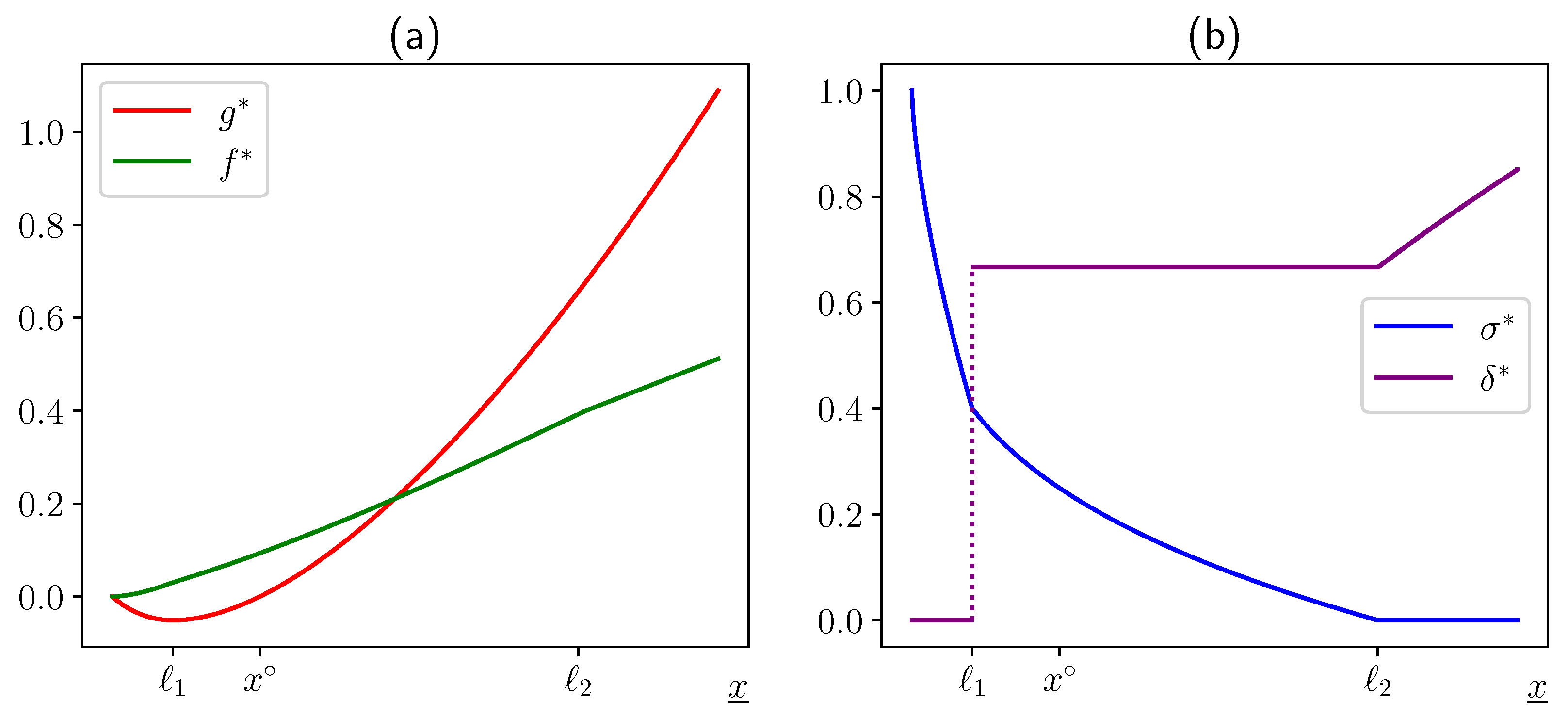
For an illustration, consider the following parameter values:

$$A=1.8,\mu =0.3,\nu =0.5,p=1.$$

Here, ${\ell }_1\approx 0.255$, $x^{\circ }\approx 0.622$, ${\ell }_2\approx 1.968$. The functional dependencies of $f^{\ast }$, $g^{\ast }$, ${\delta }^{\ast }$, ${\sigma }^{\ast }$ on the industrial investment level $\underline{x}$ are shown in Figure 1. A more realistic example is presented in the next section.

Figure 1. (a) Follower’s optimal revenue $f^{\ast }$, and optimal leader’s cost $g^{\ast }$. (b) Optimal subsidy fraction ${\delta }^{\ast }$, and optimal tax fraction ${\sigma }^{\ast }$.

6. Case Study: Water Production in Lahore

In a recent paper [24], the authors used the Cobb–Douglas production function to model a local water company in Pakistan. The water processing process includes filtering, adding chemicals, packing, and selling at the market. The amount P of produced water (measured in liters: l) in [24] was modeled as

$$P=\mathcal{A}{L}^{\mu }{M}^{\nu },$$

(53)

where L is the number of labor hours, and M is the amount of raw materials, measured in kg. The parameter values

$$\mathcal{A}=3212.468,\mu =0.3568,\nu =0.0542$$

were estimated in [24] for the real data related to local branches of Chemtronics Water Services in Lahore, Pakistan. These estimates were based on the samples of P, L, M with the following means (we show the standard deviations in brackets):

$$\overline{P}=35.7·{10}^3(\pm 1.25·{10}^3),\overline{L}=304.5(\pm 25.7),\overline{M}=903.4(\pm 36.7).$$

(54)

According to [24], the price of raw materials $p_m$ and the price of labor p are given by

$$p_m=100\mathrm{PKR}/\mathrm{kg},p=1400\mathrm{PKR}/\mathrm{hr},$$

where PKR is the abbreviation for Pakistan rupees. The price of processed water was not given in [24]. In fact, it can depend on the quantity sold, the brand, and other factors. A google query like “the price of pure (drinking) water in Lahore” gives the range from 30 to 50 rupees per liter. Let us take the lowest of these values

$$p_w=30\mathrm{PKR}/\mathrm{l}$$

as a rough approximation, since we are on the wholesale manufacturer’s side.

Instead of (53), for our model we need the dependence between the current and future amount of industrial investments; see (1). In view of (53), Formula (1) should be rewritten as follows:

$$x_{t+1}=p_w{P}_{t+1}=p_w\mathcal{A}{L}^{\mu }{\left(\frac{(1-\beta )x_t+(1+\delta )\alpha y_t}{p_m}\right)}^{\nu }=A{L}^{\mu }{((1-\beta )x_t+(1+\delta )\alpha y_t)}^{\nu },$$

$$A=\frac{p_w}{p_m^{\nu }}\mathcal{A}\approx 75086.$$

(55)

The model and the problem formulated in [24] are quite different from ours. For instance, the former did not take into account taxes, subsidies, and the market price of water. Thus, it would be interesting if our model can produce realistic results concerning, e.g., water production. Let us compute this quantity for the critical values ${\ell }_1$, ${\ell }_2$ of the industrial investments:

$$w_1:={\ell }_1/p_w\approx 17808,w_2:={\ell }_2/p_w\approx 35161,$$

and the fair production level $w^{\circ }$, corresponding to the fair industrial investment level (50):

$$w^{\circ }=x^{\circ }/p_w\approx \mathrm{33,120}.$$

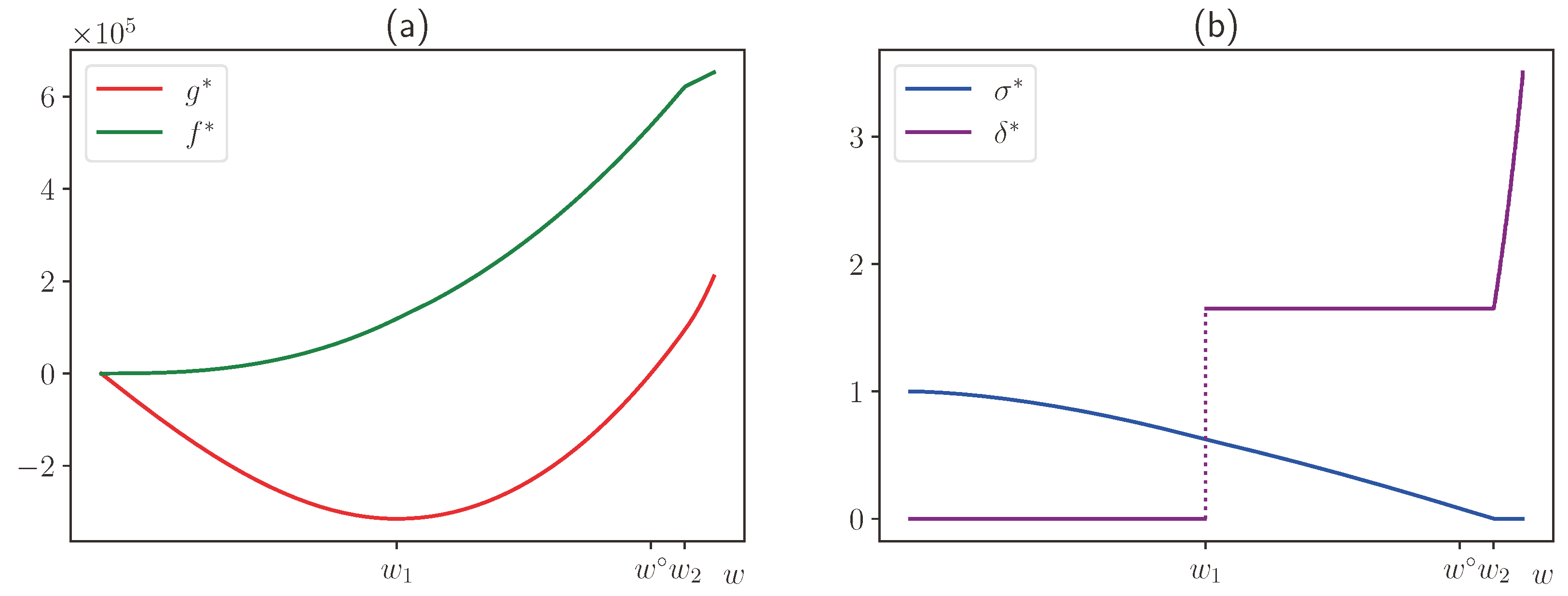
Surprisingly, this value is not far from the true average production value $\overline{P}$ given by (54), while the basic production level $w_1$ is almost twice as small. The functional dependence of $f^{\ast }$, $g^{\ast }$, ${\delta }^{\ast }$, ${\sigma }^{\ast }$ on the production level $w:=\underline{x}/p_w$ is given in Figure 2. The tax and subsidy fractions (51) in our case equal

$${\sigma }^{\ast }(x^{\circ })\approx 0.08,{\delta }^{\ast }(x^{\circ })\approx 1.65.$$

Note that the subsidy amount is quite large.

Figure 2. Prediction of the dependence of basic quantities on the amount w of water produced in Lahore. (a) The follower’s optimal revenue $f^{\ast }$, and the leader’s optimal cost $g^{\ast }$. (b) Optimal subsidy fraction ${\delta }^{\ast }$, and optimal tax fraction ${\sigma }^{\ast }$.

As was mentioned, our guess concerning the price of water $p_w=30$ PKR/l was rather rough. Let us compute the production level, the amount of raw materials and labor, corresponding to $x^{\circ }$, for $p_w$ in a certain range. The amount of production equals

$$P^{\ast }(x^{\circ }):=\frac{x^{\circ }}{p_w}={\left(\mathcal{A}{\left(\frac{\nu }{p_m}\right)}^{\nu }\right)}^{1/(1-\mu -\nu )}{\left(\frac{\mu }{p}\right)}^{\mu /(1-\mu -\nu )}{\left(\frac{p_w}{\varkappa }\right)}^{(\mu +\nu )/(1-\mu -\nu )}.$$

(56)

To compute $L^{\ast }(x^{\circ })$, we use the middle line in (49), and Formulas (46), (50) and (55):

$$\begin{array}{cc}\hfill & L^{\ast }(x^{\circ })={\left({\displaystyle \frac{1}{A{\nu }^{\nu }}}\right)}^{1/(\mu +\nu )}{\left({\displaystyle \frac{\mu }{p}}\right)}^{\nu /(\mu +\nu )}{\left({\displaystyle \frac{\mu }{1-\nu }}\right)}^{\nu /(\mu +\nu )}{(x^{\circ })}^{1/(\mu +\nu )}\hfill \\ \hfill & ={\left(\frac{\mathcal{A}}{\mu +\nu }{\left(\frac{\nu }{p_m}\right)}^{\nu }\right)}^{1/(1-\mu -\nu )}{\left(\frac{\mu }{p}\right)}^{(1-\nu )/(1-\mu -\nu )}{\left(\frac{\mu }{1-\nu }\right)}^{(1-\nu )/(1-\mu -\nu )}{p}_w^{1/(1-\mu -\nu )}.\hfill \end{array}$$

(57)

The amount of raw materials used in production at equilibrium $(x^{\ast },y^{\ast })$ is given by

$$M^{\ast }=\frac{(1-\beta )x^{\ast }+(1+\delta )\alpha y^{\ast }}{p_m}=\frac{1}{p_m}\left(1-\beta +\rho \beta \frac{\gamma }{1+\gamma }\right)x^{\ast },$$

where we used (16). But for $x^{\ast }=x^{\circ }$, using Theorem 3 and Formula (52), we have

$${\beta }^{\ast }(x^{\circ })=1,\frac{{\gamma }^{\ast }(x^{\circ })}{1+{\gamma }^{\ast }(x^{\circ })}=\nu ,\rho (x^{\circ })=\frac{1}{\mu +\nu }.$$

Thus,

$$M^{\ast }(x^{\circ })=\frac{\nu }{\nu +\mu }\frac{x^{\circ }}{p_m}=\frac{\nu }{\nu +\mu }\frac{p_w}{p_m}{P}^{\ast }(x^{\circ }).$$

(58)

Table 1 shows the dependence of $P^{\ast }(x^{\circ }$), $L^{\ast }(x^{\circ })$, $M^{\ast }(x^{\circ })$, given by (56)–(58) on the water price $p_w$ in the range $[25,40]$ (per liter).

Table 1. Predicted dependence of the optimal amounts of production, labor, and raw materials on the price $p_w$ of processed water at the fair industrial investment level $x^{\circ }$ (the case of Lahore, Pakistan).

Water Price, PKR/l ${\mathit{p}}_{\mathit{w}}$	Production, l ${\mathit{P}}^{\ast }({\mathit{x}}^{\circ })$	Labor, hr ${\mathit{L}}^{\ast }({\mathit{x}}^{\circ })$	Raw Materials, kg ${\mathit{M}}^{\ast }({\mathit{x}}^{\circ })$
25	29,164	171	961
26	29,973	182	1028
27	30,773	194	1096
28	31,564	207	1165
29	32,346	219	1237
30	33,120	232	1310
31	33,887	246	1385
32	34,646	259	1462
33	35,398	273	1540
34	36,143	287	1621
35	36,882	302	1702
36	37,614	317	1786
37	38,340	332	1871
38	39,060	347	1957
39	39,774	363	2046
40	40,483	379	2135

To compare the results predicted by Table 1 with the true average values (54), consider two lines corresponding to the production amounts of 35,398 and 36,143 L. We see that the predicted optimal amount of labor is lower than $\overline{L}$, and the predicted optimal amount of raw materials is higher than $\overline{M}$. Interestingly, in [24], the obtained optimal values of labor and raw materials (for the production level 36,000) of 334 and 688, respectively, shifted in the opposite direction.

Note that it is also possible to predict the price of water using Table 1. If we calibrate the production amount according to the average value $\overline{P}$, given in (54), then the predicted price of water will be approximately 33.5 PKR/l.

7. Conclusions

We introduced and studied a model for targeting industrial investments by using subsidies and taxes. We analyzed a Stackelberg game corresponding to the equilibrium of the dynamical system that governs the components of investor’s capital. The obtained explicit solution transparently described the strategies of the government and the investor. Based on this solution, we introduced the notion of a fair industrial investment level $x^{\circ }$, which is costless for the government. Using a case study of water production in Lahore, we showed that $x^{\circ }$ can produce realistic values for the amounts of production, labor, and raw materials. This result appears encouraging.

This paper may serve as a baseline for further development of the proposed model. Let us mention a few possible research directions.

Adding randomness, which preserves a form of asymptotic stability of the corresponding dynamical system, in principle allows stating a problem in a similar manner. However, such a problem will be much more complex, and its analysis will certainly require numerical methods to obtain quantitative results. The obtained exact solution in the deterministic case may be useful for testing such methods. A more simple case arises when only the parameters of the Cobb–Douglas production functions are randomized.

Another possibility would be to consider several investors for the same enterprise. Here, an additional problem concerns the capital sharing, and this is related to game theory. A distinct problem concerns a game between different enterprises producing the same good.

Finally, it is possible to allow the investor and/or the government to use more complex strategies. This should result in a dynamic game over a finite or infinite horizon. In addition to the inevitability of numerical methods, here, an additional significant difficulty arises: one needs to take into account the initial conditions and the horizon, if it is finite.