A Semi-Supervised Active Learning Method for Structured Data Enhancement with Small Samples

Abstract

In order to solve the problems of the small capacity of structured data and uneven distribution among classes in machine learning tasks, a supervised generation method for structured data called WAGAN and a cyclic sampling method named SACS (Semi-supervised and Active-learning Cyclic Sampling), based on semi-supervised active learning, are proposed. The loss function and neural network structure are optimized, and the quantity and quality of the small sample set are enhanced. To enhance the reliability of generating pseudo-labels, a Semi-supervised Active learning Framework (SAF) is designed. This framework redistributes class labels to samples, which not only enhances the reliability of generated samples but also reduces the influence of noise and uncertainty on the generation of false labels. To mine the diversity information of generated samples, an uncertain sampling strategy based on spatial overlap is designed. This strategy incorporates the idea of spatial overlap and uses global and local sampling methods to calculate the information content of generated samples. Experimental results show that the proposed method performs better than other data enhancement methods on three different datasets. Compared to the original data, the average ${F1}_{macro}$ value of the classification model is improved by 11.5%, 16.1%, and 19.6% relative to compared methods.

1. Introduction

In recent years, with the vigorous development of computer information technology, machine learning algorithms have been widely used in various fields. In many practical applications, high-quality training sample sets are the data basis for machine learning tasks to perform well. However, this often leads to the inability to build high-quality training sample sets for machine learning tasks and to conduct more in-depth research on machine learning algorithms in some areas where data acquisition is difficult. Therefore, it is of great significance and value to carry out learning research on small-sample data for fields where data are scarce [1].

Generally, there are some problems in small-sample data, such as small capacity and uneven distribution of labels among classes [2]. If a small set is directly used as the training sample for the model, the generalization ability of the model may deteriorate due to incomplete data information. In addition, small-sample data can be divided into structured data and unstructured data. Structured data comprise a two-dimensional relational table that is not constrained by primary and foreign keys, while unstructured data are the opposite. The traditional solution is to resample small samples of structured data from the data level so that the majority and minority samples tend to be balanced. For unstructured data research, for example, in the image field, the sample set can be expanded by adding noise, cropping, and scaling to the picture data [3]. With more in-depth research, a series of generative models has been derived. The main idea is to learn the data distribution of real samples so that the generated data can meet the scale and quality requirements of training sample sets in machine learning tasks. Among them, the variational autoencoder [4] and Generative Adversarial Network (GAN) [5] have laid the foundation for generative models. The variational autoencoder uses the idea of the variational lower bound automatically learning the data distribution of real samples under an unsupervised learning mode. In a GAN, two neural networks playing games with each other gradually learn the data distribution of real samples during the training process.

Semi-supervised learning [6] and active learning [7] have also been developed. The core idea is to use a pseudo-label allocation strategy to ensure the reliability of unlabeled samples. Semi-supervised learning uses the data information of unlabeled samples to establish a model with strong generalization ability. Active learning employs a query strategy to screen out the samples that can improve the performance of the model, label them manually, and gradually establish a high-quality sample set. If the two are used for collaborative learning, not only can the comprehensive utilization of labeled and unlabeled samples be realized, but the quality and quantity of small-sample data can also be improved. Therefore, how to use active learning strategies to mine the diverse information of unlabeled samples under semi-supervised learning is the focus of current research. This also lays a theoretical foundation for research on small-sample structured data enhancement methods presented in this paper.

To date, many excellent research results have been reported using small-sample learning for structured data, which, to a certain extent, can realize machine learning tasks with a small number of samples. However, there are still many aspects worthy of further exploration, such as how to build a more suitable generative model for small-sample structured data and how to design a more reliable pseudo-label allocation strategy for generated data. In this paper, by mining the characteristics of noble metal samples, a diversified and cross-scale classification model is developed. However, due to the high requirements for experimental equipment and resources, this approach requires a long time period and considerable amounts of human resources. This also means that it is impossible to obtain a large amount of experimental data to explore the structure–activity relationship between material properties in a short time. Therefore, the main content of this study investigates the enhancement of the quantity and quality of small-sample structured data to solve the problems of the lack of diversified information such as small data capacity and uneven distribution among label classes, then build a high-quality sample set.

2. Related Work

In recent years, with the rapid development of information technology, mining diversified information from sample data to build high-quality sample sets has become a prerequisite for machine learning tasks [8]. There are currently two main approaches used in research on small-sample structured data, namely small-sample learning based on model algorithms and small-sample learning based on data enhancement [9,10,11].

(1) Small-sample learning based on model algorithms mainly focuses on learning the characteristics of small-sample data from training tasks and establishing a model with strong generalization ability. There are two ways to implement this approach; one is to map the existing space to a lower-dimensional space, thereby adapting to the scale of small-sample data during training, and the other is to narrow the gap relative to the real model algorithm, such as by sharing multi-task learning parameters [12]. Additionally, a method based on optimization algorithms has been proposed. This method optimizes the hyperparameters of the model, usually by including grid search algorithms [13] and random search algorithms [14]. Meta learning [15] or transfer learning [16] can also be used to optimize the parameters of the model algorithm. The core idea is to train the parameters of the model on other learning tasks and use this model as the base model to fine tune the parameters for the current learning tasks. For example, Huang, L. [17] proposed a two-segment multi-data-source migration method. First, the data information of each source sample is extracted using confidence classification rules. Then, according to domain consistency rules, the weights of different sources are set. Finally, when there is a significant difference between the source sample set and the target sample set, the model can be adjusted to make it suitable for the current learning task. However, when screening and designing auxiliary sample sets, the differences among various training sets can still lead to deviations in the results of current learning tasks. Therefore, small-sample learning methods based on model algorithms are difficult to apply in practical scenarios and are not universally applicable.

(2) Small-sample learning based on data enhancement primarily aims to enhance the quantity and quality of the original sample set through sampling and generation, thereby compensating for the shortcomings of the aforementioned small-sample learning methods. According to the enhancement methods of sample data, these can be divided into enhancement methods based on data synthesis and enhancement methods based on data labeling.

(i) The enhancement method based on data synthesis primarily involves small-sample data enhancement by synthesizing new samples. Data synthesis methods are divided into resampling methods and generating methods.

The core idea of the resampling method is to sample from the original sample set to address the issues of small sample size and uneven class distribution. Common resampling methods include undersampling [18], oversampling [19], and hybrid sampling [20]. Among these, the approach of the undersampling method is to select the same number of majority-class samples as the minority classes to achieve class balance. The simplest undersampling method is random undersampling, which involves the random deletion of majority-class samples. However, this may result in the loss of important information from the sample set, thereby affecting the final precision of the model. The oversampling method aims to balance the classes by adding samples to the minority class. The simplest oversampling method is random oversampling. It is mainly a resampling algorithm that randomly copies a few samples from the data level. This kind of method not only keeps the data structure of the original sample set but also improves the problem of uneven distribution of small sample categories when enhancing the data of small samples. In addition, if it is applied to the classification model, it can also improve the generalization ability of the model to a certain extent. However, because it is a complete copy of the original sample, the same sample will train the model repeatedly, which leads to an overfitting phenomenon due to the influence of skewness distribution. Hybrid sampling combines oversampling and undersampling methods, thereby compensating for the shortcomings of using either method alone. For example, Tsai, C. [21] proposed a sub-sampling method based on clustering, which achieves class balance by clustering majority-class samples and deleting unrepresentative samples. Chawla, N.V. [22] proposed an interpolation-based oversampling algorithm called SMOTE, whose core idea is to balance the sample set by synthesizing a few samples. This method borrows the idea of KNN, assuming that a few samples are x, and, according to the idea of the KNN algorithm, randomly selects a sample point (y) among the K nearest neighbors and randomly selects a point on the line between sample points x and y as a new composite sample. The SMOTE algorithm can effectively reduce the risk of model overfitting. However, this way of synthesizing minority samples does not consider the influence of majority samples. Therefore, to a certain extent, the overlapping degree of sample sets between different classes is increased, making the synthesized noise data blur the sample boundaries and increasing the burden of the model. Han, H. [23] proposed the Borderline-SMOTE algorithm based on the SMOTE algorithm. First, the algorithm divides a few samples into three categories, namely safe, noise, and danger, and uses the SMOTE algorithm to synthesize only danger samples near the decision boundary. The Borderline-SMOTE algorithm synthesizes representative sample points by removing noisy data and interpolating near the boundary and, at the same time, reduces the degree of overfitting of the model. When synthesizing new sample points, the original sample set can maintain class equilibrium by constraining a few classes at the boundary or the among nearest neighbors of any sample. He, H [24] proposed an Adaptive Synthetic (ADASYN) sampling approach. Its core idea is to take the distribution density of samples as the measurement criterion of synthetic data quantity so as to achieve the purpose of balancing datasets. The ADASYN algorithm not only considers the influence of a few kinds of samples but also does not depend on a specific value in the process of self-adaptively generating new samples, so it has good applicability.

The core idea of generative methods is to generate data distributions similar to real samples, thereby enhancing the quantity and quality of small-sample data. Among these methods, the most commonly used generative model is GAN. GAN is a data generation model based on the idea of adversarial training, providing a new way to address the issue of small-sample data [25]. In the training process of GAN, two neural networks are used for adversarial learning, which results in faster training speeds and higher-quality generated samples. However, during training, there are often issues such as mode collapse and gradient vanishing.

For this reason, Yu, H. and others have proposed various derivative models of GAN [26]. For example, the Wasserstein Generative Adversarial Network (WGAN) [27] changes the measure of data distribution to the Wasserstein distance, effectively addressing some of the problems associated the original GAN. However, directly truncating the update parameters of the discriminator within a fixed interval can lead to difficulties in the convergence of the loss value. Therefore, the Wasserstein Generative Adversarial Network with Gradient Penalty (WGAN-GP) proposed by Jin Q. [28] introduces a gradient penalty to improve the convergence issue in WGAN training. Additionally, Wang, Y. [29] proposed a Conditional Generative Adversarial Network (CGAN), which alters the training mode from unsupervised learning to semi-supervised learning by introducing constraints to guide the data generation process. Building on CGAN, Kang, M. [30] proposed the Auxiliary Classifier Generative Adversarial Network (ACGAN), which improves the quality of generated samples by reconstructing category labels.

(ii) The enhancement method based on data labeling primarily involves enhancing small-sample data by assigning reliability labels to unlabeled samples. However, the cost and effort of labeling sample sets are very high. To address the issue of having few reliability labels in small-sample data, semi-supervised learning and active learning have been developed.

Semi-supervised learning is an indispensable part of the field of machine learning, and its core idea is to enhance the scale and quality of small sample sets by utilizing the information from unlabeled samples. During training, it does not require the labels of the unlabeled samples to be correct but, rather, moves towards the correct direction based on assumptions about data distribution. Common semi-supervised learning methods include self-training [31] and co-training [32]. The idea behind the self-training method [33] is to initially use labeled samples to train a base classifier. Then, the base classifier is used to predict the labels of the unlabeled samples. Samples with high label reliability are selected to retrain the base classifier, along with the initial labeled samples, and this process is repeated continuously until a stopping condition is met. Although this method is simple and easy to implement, it completely relies on the predictions of its own base classifier, making it prone to labeling errors, which can ultimately lead to a decrease in the precision and generalization ability of the classifier. The main idea of graph-based semi-supervised learning [34] is to represent sample points as nodes in a graph, thereby preserving the geometric structure information of the samples. First, the connection mode of the graph is selected, and the distances between samples are calculated. Second, the edges of the graph are weighted. Finally, the objective function is solved. Although the structure of this method is clear, the storage cost of graphs is high, and there is a strong dependence on the data.

The core idea of active learning is to use query strategies to reduce the model’s dependence on the training sample set in learning tasks. During training, the most informative samples are selected using a query strategy and labeled by experts. This process is repeated until the stopping conditions are met. Common query strategies include least confident sampling [35] and margin sampling [36]. Active learning is a method aimed at reducing the labeling cost of small-sample data. Compared to semi-supervised learning, active learning enhances supervisory information through specific query criteria, thereby improving the generalization ability of the classification model while reducing costs. First, the method queries the samples that are most beneficial for improving the classifier’s performance and submits them to experts for labeling. These samples are then added to the initial sample set to retrain the classifier. This process is repeated until the stopping condition is met. The query criterion of active learning is akin to a sampling strategy, with the main idea being to measure the uncertainty of unlabeled samples to select those with the highest information content for manual labeling. However, it is challenging to perform queries in active learning when there is a lack of training samples. Therefore, to enhance the effectiveness of active learning, it is often combined with other learning tasks, such as semi-supervised learning.

The core idea of semi-supervised active learning is to use semi-supervised learning and active learning for collaborative training. In this process, the query strategy of active learning compensates for the problem of low reliability caused by false labels in semi-supervised learning due to the lack of supervision information. Conversely, semi-supervised learning directly utilizes unlabeled samples for training, addressing the issue of insufficient query capability in active learning caused by a lack of reliable samples. Xu, H. [37] proposed a semi-supervised active learning method based on a support vector machine, which combines the ternary training method of semi-supervised learning with the query strategy of active learning. This method uses the information from unlabeled samples to enhance the model’s recognition and generalization abilities. Therefore, information mining of small sample data under semi-supervised active learning is a hot research topic at present and is also the focus of this paper.

The main contributions of this paper are outlined as follows: (1) Addressing the issues of the small capacity of structured data and uneven class distribution, this paper investigates the generation of adversarial networks and proposes a supervised generation method for structured data. Based on the original GAN, the distance distribution measure is replaced, and a gradient penalty and class label reconstruction are introduced to improve the neural network structure and training process. Experimental results show that this method not only resolves the issues of mode collapse and gradient vanishing during the training of the original GAN but also enriches the diversity of information in small-sample structured data. (2) The quality of the sample set constructed by the abovementioned generation method is unstable, and the noise data in the sample set increases the burden on the classification model, weakening the overall recognition ability. Therefore, this paper studies semi-supervised active learning and proposes a cyclic sampling method based on semi-supervised active learning. First, to enhance the reliability of pseudo-labels, an active learning framework based on semi-supervision is designed. Then, an uncertain sampling strategy is proposed to mine diverse information from the generated sample set. Experiments show that this method not only enhances the reliability of pseudo-label generation but also constructs a higher-quality sample set by sampling global and local uncertainties.

The organizational structure of this paper is outlined as follows: In Section 3, we introduce the Wasserstein Auxiliary Generative Adversarial Network (WAGAN) model. In Section 4, we discuss the Semi-supervised and Active-learning Cyclic Sampling (SACS) method. Section 5 reports on experiments and results, and Section 6 presents our conclusions.

3. Wasserstein Auxiliary Generative Adversarial Network (WAGAN) Model

3.1. Framework of WAGAN Data Generation Method

Addressing the problem of limited capacity in structured data and the unbalanced distribution of categories, this paper proposes a structured data generation method called WAGAN. Based on the original GAN, this method combines the characteristics of multiple classification tasks and improves the algorithm’s principles, the neural network structure, and the training process of the model. It has been proven that WAGAN not only mitigates the gradient-vanishing and mode-collapse issues of the original GAN during training but also enriches the diversity of information in small-sample structured data.

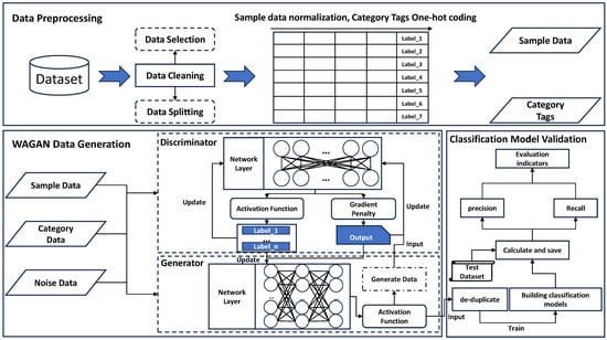
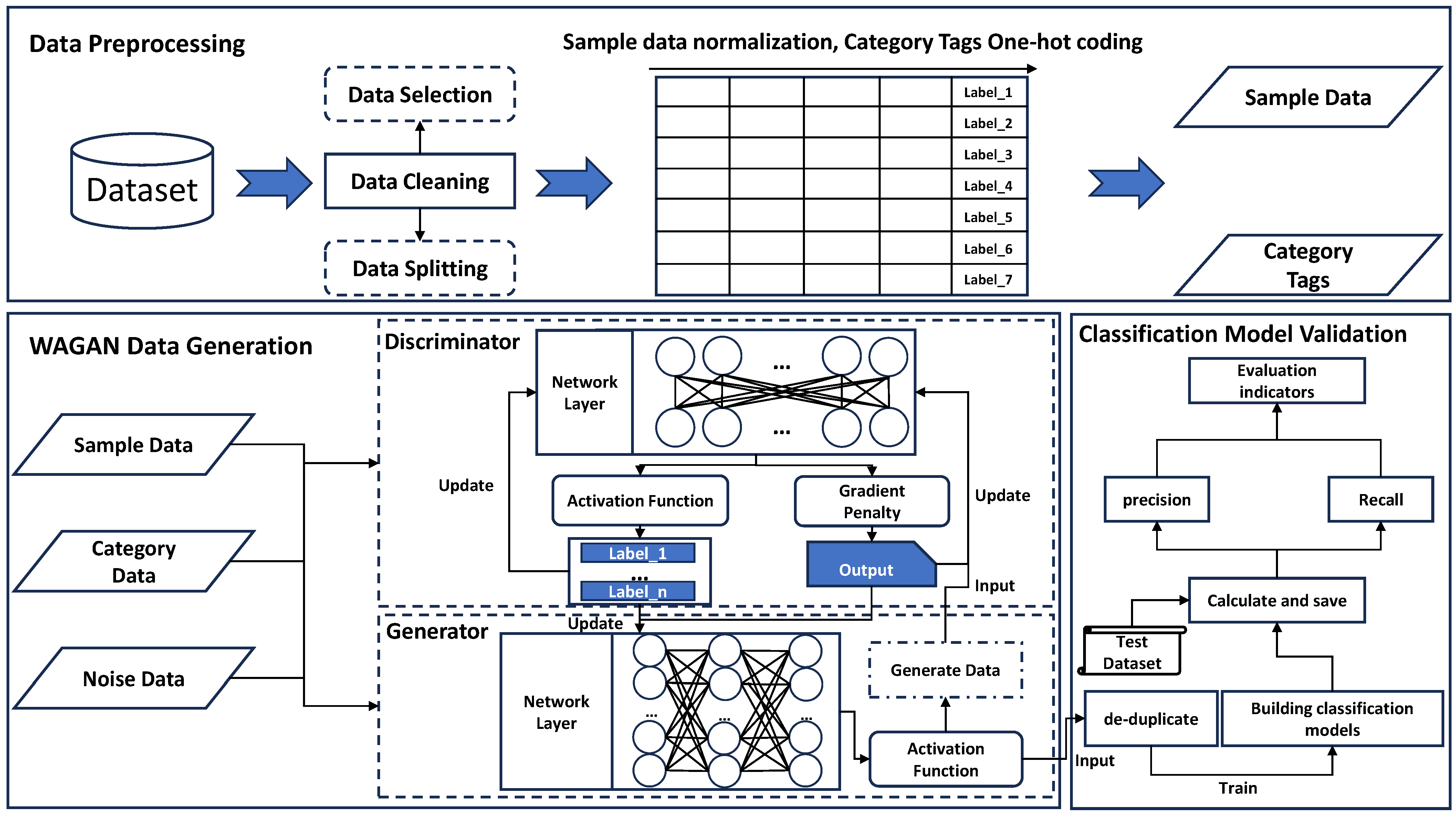
The overall structural framework of the WAGAN data generation method is shown in Figure 1. It is mainly divided into the following three parts: (1) Data Preprocessing Module: First, data cleaning is performed on the original sample set. Then, Z-score standard normalization and one-hot encoding are applied to the features and category labels of the sample data to avoid the influence of outliers and feature dimensions on subsequent generation modules. Finally, a standardized training sample set is obtained. (2) WAGAN Data Generation Module: The preprocessed sample data and category labels are fed into the WAGAN model. Through the alternate training of the generator and discriminator models, the data distribution of the original sample is learned. Finally, the trained model is used to generate sample data for specified categories. (3) Classification Model Verification Module: First, to prevent duplicate samples from affecting the classification model, the generated data are deduplicated. Then, they are sent to the classification model as a training sample set for training. Finally, the test set is used to calculate the precision and recall rate of the classification model, which is used to verify the quality of the data generated by WAGAN.

Figure 1. Architecture of WAGAN data generation method.

3.2. Principle of the WAGAN Model

The WAGAN model is an improved supervised generative adversarial network model based on the original GAN. There are two main factors that affect the effectiveness of GAN data generation, namely the unreasonable fluctuation of distance distribution measures (such as Jensen–Shannon divergence or Kullback–Leibler divergence) and the lack of diversity in samples generated under unsupervised modes. Therefore, based on small-sample structured data, this paper improves the original GAN model algorithm as follows:

(1) By changing the distance distribution metric to the Wasserstein distance instead of the original GAN distance distribution metric, the WAGAN model addresses the problem of unreasonable fluctuations in the distance distribution metric when the sample data distributions have no overlap or a small overlap. The original GAN can cause gradient vanishing or mode collapse during training. This problem primarily arises because, when the data distributions of two samples have no overlap or the overlap is negligible, the distance distribution measure (Jensen–Shannon divergence) of GAN suddenly changes into a constant term, causing the generator’s gradient to drop to zero. The distribution curve of the Wasserstein distance is more continuous and smooth, so it does not become a constant term when there is no overlap or only a small overlap in data distribution. This allows it to be resolved using the gradient descent method, ultimately solving the issues of gradient vanishing and mode collapse in the original GAN during training.

(2) By changing the loss function, the model is transformed from an unsupervised model into a supervised model using the idea of class label reconstruction, taking the class label as the supervision information for the generator. This enriches the diversity of generated samples. After changing the distance distribution metric, the discriminator no longer performs the binary classification task but instead becomes a regression task for approximate fitting. Therefore, a gradient penalty strategy is integrated into this approach to maintain the continuity of the discriminator’s output.

Based on the above-mentioned measures to improve the distance distribution metric, the problem caused by unreasonable Jensen–Shannon Divergence fluctuations in the original GAN is mitigated to a certain extent. However, when using the Wasserstein distance to calculate data distribution, its value is continuous and differentiable, so it is necessary to ensure the continuity of the discriminator’s output parameters during training. To address these issues, WGAN and WGAN-GP have introduced improvements. WGAN uses weight clipping to maintain the continuity condition, but this limits the parameter range of the discriminator updates and may eventually lead to gradient explosion and non-convergence of the loss value. Therefore, this paper adopts the algorithmic approach of WGAN-GP and introduces gradient penalty, which not only ensures the continuity of the discriminator’s output parameters but also avoids the adverse effects of aggressive weight clipping in WGAN. However, the unsupervised learning mode lacks supervised information, leading to random generated samples. To overcome this, this paper introduces the idea of label reconstruction based on a multi-classification learning task and proposes the core algorithm of the WAGAN data generation method, namely the multi-classification label reconstruction algorithm with gradient penalty.

3.3. Neural Network Structure of WAGAN Model

The model structure of WAGAN consists of a generator model and a discriminator model. To avoid training difficulties or overfitting caused by a complex model structure, the neural network structures of both models are set to be fully connected.

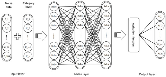
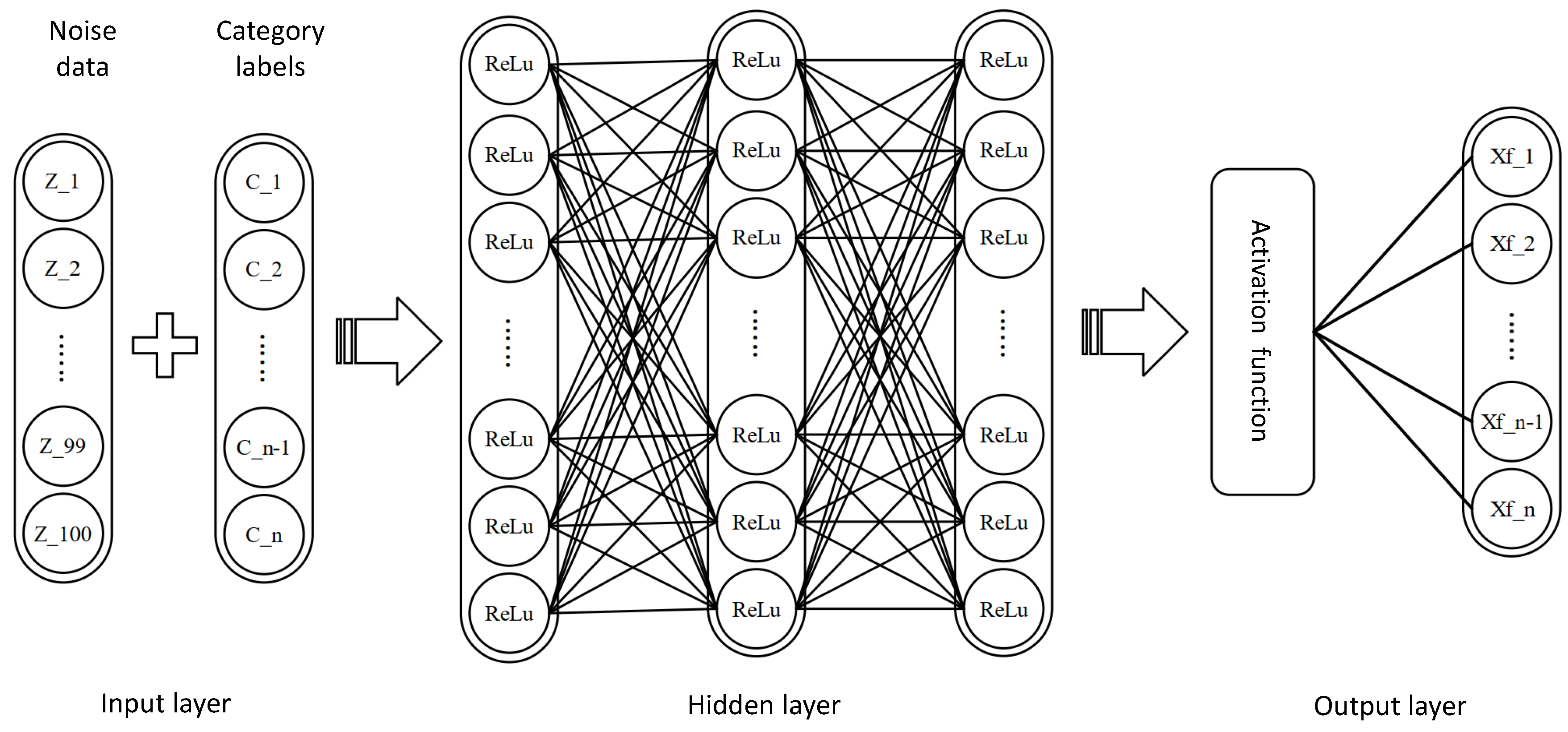
The neural network structure of the WAGAN generator model is shown in Figure 2. It includes the following three main parts: (1) One input layer that contains two components, namely random noise data and category labels. The dimensionality of the noise data is 1 × 100 dimensions. (2) Three hidden layers: The total number of neurons is 1024 × 128 × 64. Each hidden layer uses the LeakyReLU activation function. The specific numbers of hidden layers and neurons are set according to the training stability of the model, as determined by multiple experiments and comparison results. (3) One output layer: The output layer of the model uses the Tanh activation function, and the output is the generated sample set.

Figure 2. The neural network structure of the generator.

The neural network structure of the WAGAN discriminator model is shown in Figure 3. It includes the following three parts: (1) An input layer, including real sample data, generated sample data, and category labels. The sample data are not concatenated with category labels. (2) Two hidden layers: The total number of neurons is 64 × 32, and each layer adopts the LeakyReLU activation function, similar to the generator model. The method of setting the number of neurons in the hidden layers is the same as in the generator model, selected according to the convergence and stability of the model. (3) An output layer containing sample data and category labels. To maintain the continuity of the discriminator’s output, the Sigmoid activation function is removed from the output layer of the sample data, and a gradient penalty is introduced. The output layer for category labels uses the softmax activation function for multi-classification tasks.

Figure 3. The neural network structure of the discriminator.

4. Semi-Supervised and Active-Learning Cyclic Sampling (SACS) Method

The WAGAN data generation method improves the limited capacity of structured data and the uneven distribution of label classes to some extent, but it does not achieve the expected results. According to analysis, there are two main reasons, the first of which is the reliability of false labels. The category labels generated by the samples are not absolutely reliable, which affects the trend of correctness in model training to some extent. Secondly, the amount of information contained in the sample data is unstable. When addressing the problem of imbalance among label classes, although WAGAN can generate sample data of specified categories, the information content of the samples generated each time is unstable. This means their contribution to the classification model varies, which eventually leads to variability in the quality of the constructed sample set. Therefore, to solve the above problems, this paper proposes the SACS method. Its main purpose is to increase the reliability of false labels and extract diverse information from sample data, thereby building a high-quality sample set. Compared with the traditional resampling method, this method does not rely on the reliability of pseudo-labels but samples the uncertainties in the sample data within the framework of semi-supervised collaborative active learning, aiming to construct high-quality sample sets. Experiments show that the sample set constructed by this method not only contains the largest amount of information but also reduces the dependence of the classification model on sample data.

4.1. Framework of SACS

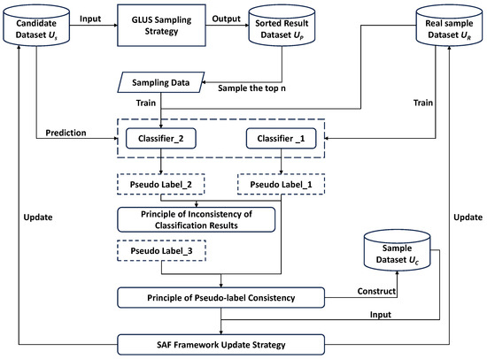
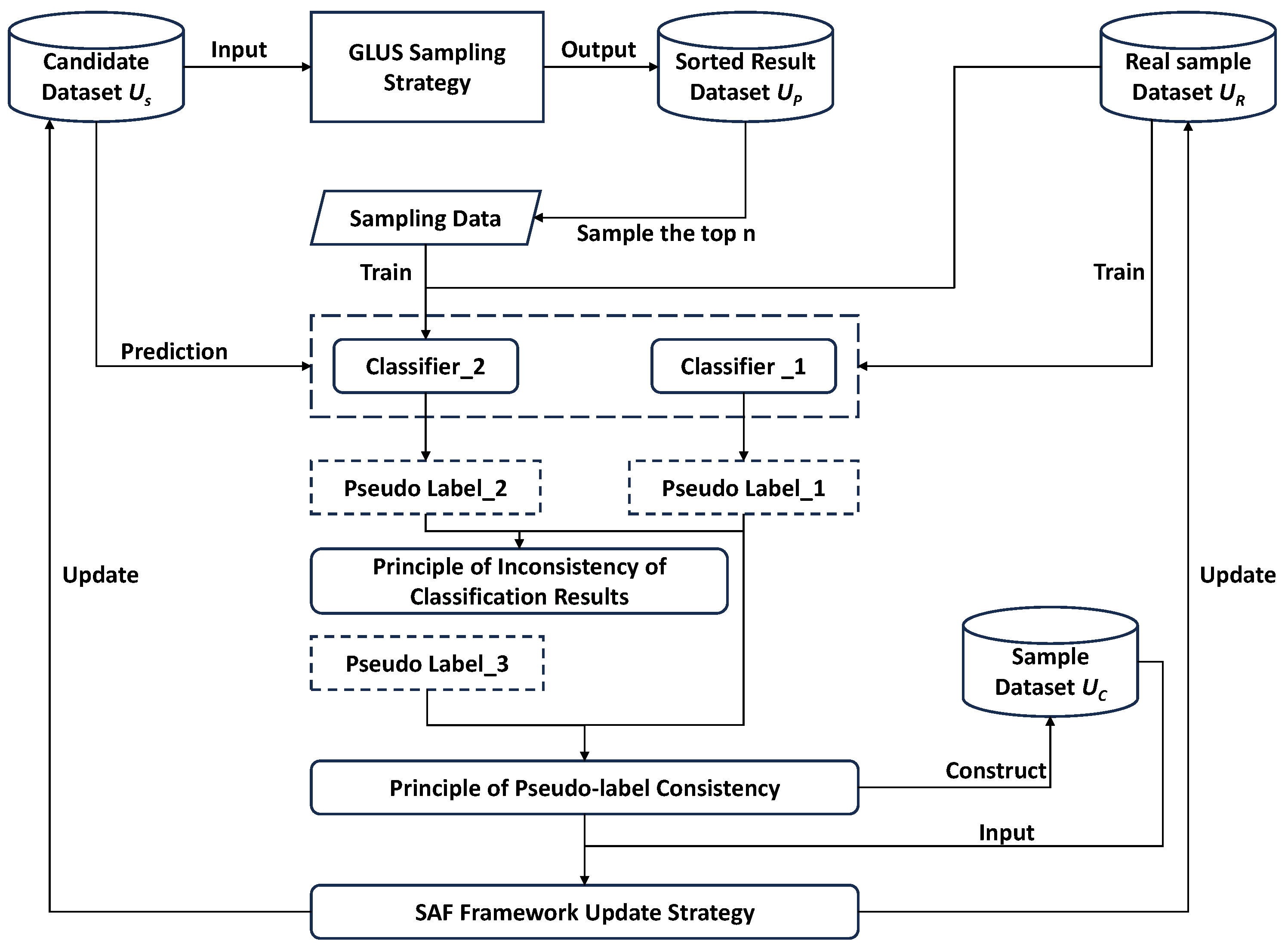
The overall structural framework of SACS is shown in Figure 4 and includes the following two core components: SAF and Global and Local Uncertainty Sampling (GLUS) based on spatial overlap. First, the samples in the candidate set are sorted according to the amount of information using the GLUS sampling strategy, and the sorted result set is obtained. Then, the first n samples of the sorted result set are sampled and trained, together with the real samples, to train classifier_2, while the real sample set is used to train classifier_1. Next, the sample data are selected according to the inconsistency principle of the prediction results of the candidate sets obtained by the two classifiers, and the classification pseudo-label is assigned according to the prediction results of samples selected by classifier_1. After that, based on the consistency principle of classified pseudo-labels and WAGAN-generated pseudo-labels, the sampling level of samples is set, and the sampling sample set is constructed. Finally, the real sample set and candidate set are updated using the update strategy of the SAF, and the cycle iteration is carried out until the sample-number threshold is met.

Figure 4. Architecture of SACS.

4.2. Framework of Semi-Supervised Active Learning

As shown in Figure 5, the SAF combines semi-supervised learning with active learning, and its core aim is to enhance the reliability of pseudo-labels through the application of two principles and an update strategy, thus enriching the diversified information of the sample data. First, according to the inconsistency of the results from the two classifiers, the samples are assigned pseudo-labels. Then, the sampling level of samples is set according to the principle of consistency between generated pseudo-labels and classified pseudo-labels, and the sampling sample set is constructed.

Figure 5. Construction diagram of SAF.

Finally, according to the update strategy of the SAF, the candidate set and the real sample set are updated, and this cycle iterates until the set threshold is reached. Both classifier_1 and classifier_2 in the SAF adopt the XGBoost classification model because the XGBoost model adds a regularization term and second-order Taylor expansion to the loss function, which can effectively prevent overfitting and make the model’s loss more accurate. In addition, the loss function can be customized, and more complex, structured data can be learned by more detailed tuning of hyperparameters, which not only provides good scalability but also helps build a strong classification model for small-sample structured data.

4.3. Uncertainty Sampling Strategy Based on Spatial Overlap

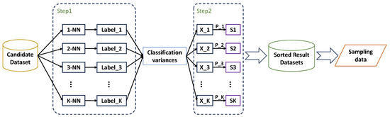
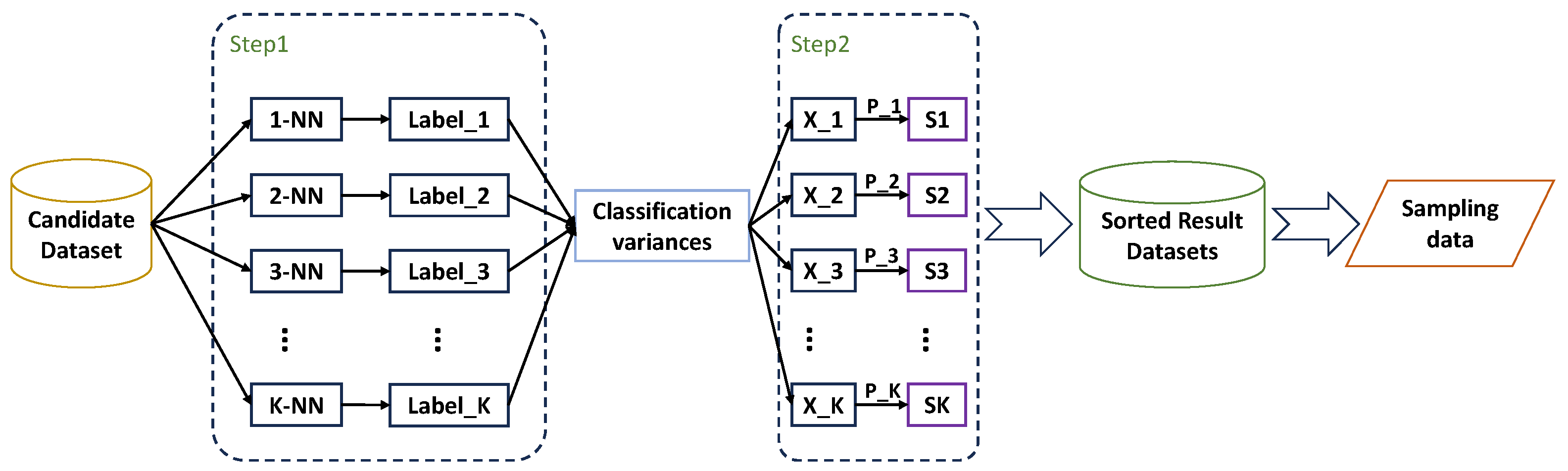
The most commonly used strategies for uncertainty measurement are the inconsistency of prediction results from multiple models and the maximum entropy of models for predicted samples. To better mine the uncertain information of sample data, this paper adopts these two methods to carry out global spatial sampling and local spatial sampling, respectively, and overlaps the sample set space to sort, finally obtaining the sorted result set based on the amount of information. The structure of the GLUS sampling algorithm is shown in Figure 6.

Figure 6. Structural diagram of GLUS sampling algorithm.

(1) Global spatial sampling is implemented in two parts. The first part involves constructing a committee set comprising 10 K-valued Gaussian Weighted K-Nearest Neighbor (GWKNN) algorithms that are used to predict the categories of all samples in the candidate set to obtain the classification results of samples. The second part involves calculating the classification difference value of predicted samples. According to the committee voting method, the K-NN classifier set is voted on, and the difference value of samples is calculated based on the inconsistency of voting results. The core content of the constructed committee set is realized using the Gaussian weighted K-NN algorithm. The basic principle of the KNN classification algorithm is to calculate the K nearest distances between known sample points and current predicted sample points and select the category with the highest frequency as the predicted category of the current samples according to the categories of the K sample points. However, the unbalanced distribution of sample data easily leads to the concentration of most surrounding sample points, causing calculation errors. This paper uses the Gaussian function weighted K-NN algorithm to optimize the weights of samples at different distances; then, the classification result set of predicted samples is obtained. The value of K directly affects the prediction probability of the final category, so choosing the value of K is key to the correct classification of the KNN algorithm. Based on this, this paper incorporates the committee voting method to vote on the classifier results of 10 K values, i.e., K∈ {1,2,3, …, 10}. First, the KNN classifier set provides the classification label of each predicted sample ($z_i$) and denotes it as $\{c^{1-NN},c^{2-NN},c^{3-NN},\dots ,c^{10-NN}\}$. Secondly, the difference value ($S_1\left(z_i\right)$) of each predicted sample ($z_i$) is calculated based on the differences in classification results, that is, if there are m different classification results, the classification difference value of the sample is m. Finally, the predicted samples are sorted from largest to smallest according to their classification difference values ($S_1\left(z_i\right)$), yielding the preliminary sorting result set of $Z=\{z_1,z_2,z_3,\dots ,z_n\}$.

(2) Local spatial sampling consists of three main steps. First, the global samples are sorted according to the classification difference value based on the results of the global sampling. Secondly, when the classification difference values of sample data are the same, the posterior probability and entropy values are calculated using the Random Forest Maximum Entropy Sampling algorithm of the random forest model. Finally, according to the classification difference value and entropy value, the final uncertainty measurement index of each set of sample data is calculated, and the ranking result set based on the amount of information is obtained. After obtaining the classification difference value of each prediction sample, the classification difference value of multiple samples may be the same. Therefore, to measure the uncertainty of sample data when the classification difference value is the same, this paper introduces local uncertainty sampling of prediction samples using the entropy value of the random forest. Random forest is a classical model based on the bagging algorithm. Its main idea is to construct n different weak classifier models by randomly selecting samples from the original sample set and obtain the final categories according to the voting results.

5. Experiments and Results

This chapter introduces the experimental data and evaluation indices. Subsequently, a parameter-tuning experiment and data-scale bottleneck experiment are conducted using WAGAN. Finally, experiments related to the SACS cyclic sampling method are analyzed, and the effectiveness and feasibility of the data enhancement method proposed in this paper are verified through comparative experiments.

5.1. Experimental Data and Evaluation Indicators

In this paper, three datasets are used to verify the effectiveness of the WAGAN+SACS data enhancement method. These three datasets are derived from the KEEL database “https://sci2s.ugr.es/keel/datasets.php (accessed on 30 July 2024)” and our noble metal project. Among them, the KEEL database’s glass dataset and yeast dataset serve as the base datasets. Samples are randomly selected and divided to create the unbalanced datasets for this experiment. The specific parameters of the three datasets are shown in Table 1.

Table 1. Dataset parameter information.

Dataset	Source	Quantity	Attribute	Category	Imbalance Ratio
glassw	KEEL	214	9	6	23.4
yeastw	KEEL	1484	8	10	7.1
noble metal	project	5525	134	46	15.4

Usually, the evaluation index of models in multi-classification tasks is based on the confusion matrix. The confusion matrix is the core calculation used to measure the recognition ability of a model. The confusion matrix for binary classification tasks [38] is shown in Table 2.

Table 2. Confusion matrix for binary classification task.

Confusion Matrix	Predicting Label Values
(Binary Classification Task)	Positive Example	Counterexample
Positive Example	TP	FN
Counterexample	FP	TN

The confusion matrix for multi-classification tasks is essentially an extension of the binary classification confusion matrix. Compared to binary classification tasks, multi-class tasks divide positive and negative instances according to categories. As shown in Table 3, $c_{ij}$ indicates the number of samples, that is, the number of samples with the actual label ($clas{s}_i$) and the predicted label ($clas{s}_j$).

Table 3. Confusion matrix for multi-classification task.

Confusion Matrix	Predicting Label Values
(Multi-Classification Task)	Class_1	Class_2	Class_3	…	Class_m
class_1	$c_{11}$	$c_{12}$	$c_{13}$	…	$c_{1m}$
class_2	$c_{21}$	$c_{22}$	$c_{23}$	…	$c_{2m}$
class_3	$c_{31}$	$c_{32}$	$c_{33}$	…	$c_{3m}$
…	…	…	…	…	…
class_m	$c_{m1}$	$c_{m2}$	$c_{m3}$	…	$c_{mm}$

Based on the analysis of confusion matrices of two-class tasks and multi-class tasks, some evaluation indices are derived. The most commonly used are the precision rate ($Pr{e}_i$) and recall rate ($Re{c}_i$). The precision rate and recall rate of a single class instance in two classes and multiple classes are shown in Equations (1) and (2), respectively. In order to better evaluate the recognition performance of different models in multi-classification tasks, this paper introduces $F{1}_{macro}$ to weigh and harmonically average the precision rate and recall rate, that is, first calculate the $F1$ value of each class, then solve its average value, as shown in Equations (3) and (4).

$$\begin{array}{c}\hfill Pr{e}_i={\displaystyle \frac{TP}{TP+FP}}={\displaystyle \frac{c_{ii}}{{\sum }_{i=1}^{i=m}{c}_{ij}}}\end{array}$$

(1)

$$\begin{array}{c}\hfill Re{c}_i={\displaystyle \frac{TP}{TP+FN}}={\displaystyle \frac{c_{ii}}{{\sum }_{j=1}^{j=m}{c}_{ij}}}\end{array}$$

(2)

$$\begin{array}{c}\hfill F{1}_i={\displaystyle \frac{2\ast Pr{e}_i\ast Re{c}_i}{Pr{e}_i+Re{c}_i}}\end{array}$$

(3)

$$\begin{array}{c}\hfill F{1}_{macro}={\displaystyle \frac{1}{n}}\sum _{i=1}^{n}F{1}_i\end{array}$$

(4)

5.2. WAGAN Model Parameter Tuning

The training of the WAGAN model is divided into generator training and discriminator training. However, the relative training degree of these two parts in the adversarial process has a significant impact on the stability of the entire model, thereby affecting the final data generation quality. If the discriminator is trained too well, the gradient of the generator may vanish, and the loss value does not converge. Conversely, if the discriminator is not trained sufficiently, the gradient of the generator is inaccurate. Therefore, in this section, we tune the model’s hyperparameters based on the training degree of each component.

In this experiment, first, the batch sample number ($Batch\_size$) is set to 128, the training period of the entire model is recorded as $Epoch$, and the training ratio of the discriminator to the generator is recorded as $D\_t$. Then, the stability of the model during training is observed by changing the values of $Epoch$ and $D\_t$. Finally, experiments on the stability of model training are conducted on three datasets.

When $Epoch$ = 10, the WAGAN model begins to converge. However, as $Epoch$ increases further, the loss value of the model starts to oscillate, leading to training collapse. The convergence of the model on the three datasets when $Epoch$ = 10 is shown in Table 4.

Table 4. Convergence of WAGAN Model.

Dataset	D_t Value
	1	2	3	4	5	6	7	8	9	10
glassw	×	×	×	×	✓	✓	✓	✓	✓	✓
yeastw	×	×	×	×	✓	✓	✓	✓	✓	✓
noble metal	×	×	×	×	✓	✓	✓	✓	✓	✓

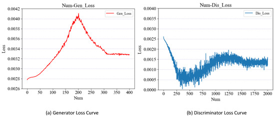
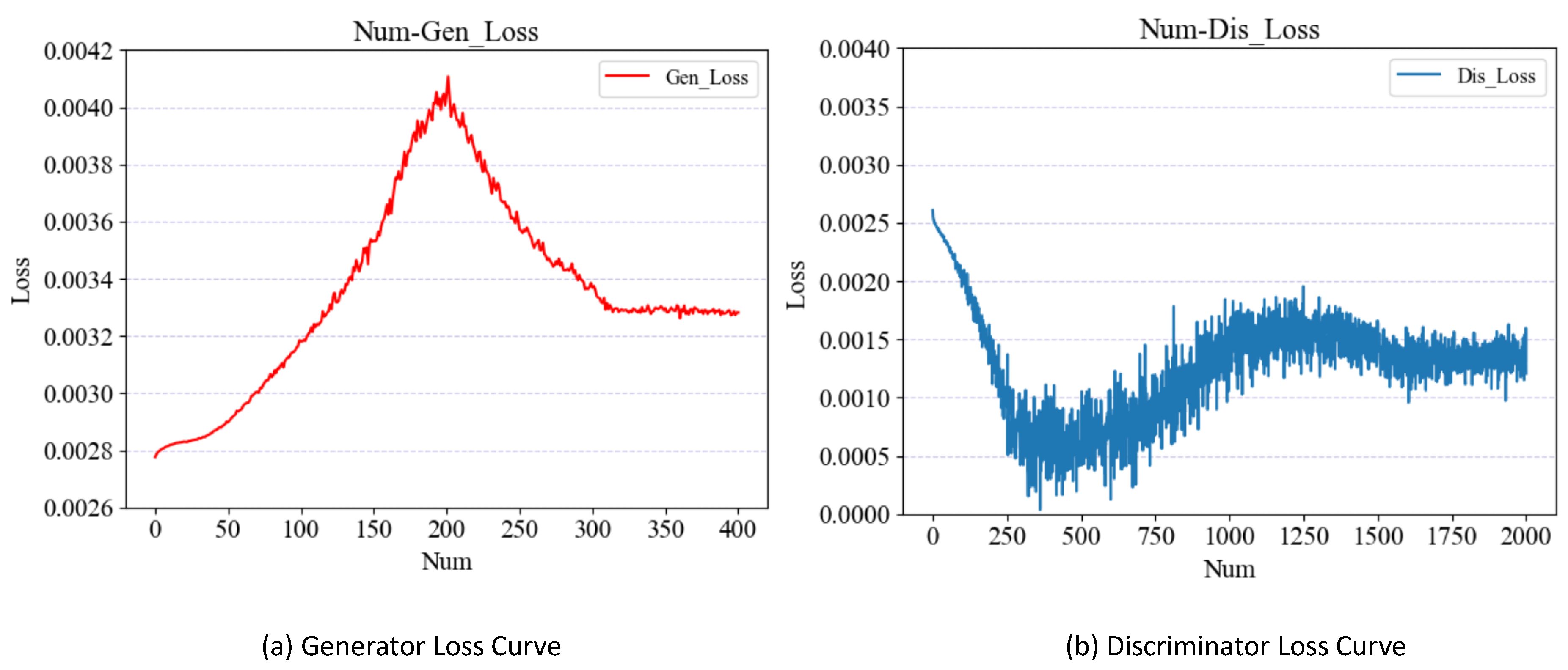
As shown in Table 4, when $Epoch$ = 10 and $D\_t$ = 5, the WAGAN model can reach a convergence state on the glassw dataset, yeastw dataset, and noble metal dataset. Taking the noble metal dataset as an example, when the generator and discriminator are trained 300 times and 1500 times, respectively, the loss-value curves of the two models begin to converge and gradually stabilize. The loss-value curves of the WAGAN generator and discriminator on the noble metal dataset are shown in Figure 7.

Figure 7. Loss-value variation curve of the WAGAN model.

From the convergence analysis of the above model, it is evident that when $Epoch$ = 10 and $D\_t$ = 5, the model begins to converge. However, as the value of $D\_t$ increases, the WAGAN model tends to be over-trained, resulting in model overfitting. Therefore, to evaluate the impact of the discriminator’s training degree on the generator, relevant experiments are conducted to determine the optimal value of $D\_t$.

In this experiment, the original dataset is first divided into a training set and a test set in a 70%-to- 30% ratio. Subsequently, based on different values of $D\_t$ during training, data are generated by the generator during each iteration, ensuring that the total amount of generated data matches the number of times the generator is trained. Finally, both the original training set and the generated data are used as the training data for classification models. The experiments evaluate the optimal value of $D\_t$ across five classification models and three datasets using ten-fold cross-validation. The tested classifier models include Decision Tree (DT), Random Forests (RF), eXtreme Gradient Boosting (XGB), Multilayer Perceptron (MLP), and Light Gradient Boosting Machine (LGBM).

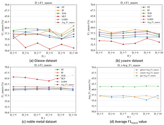
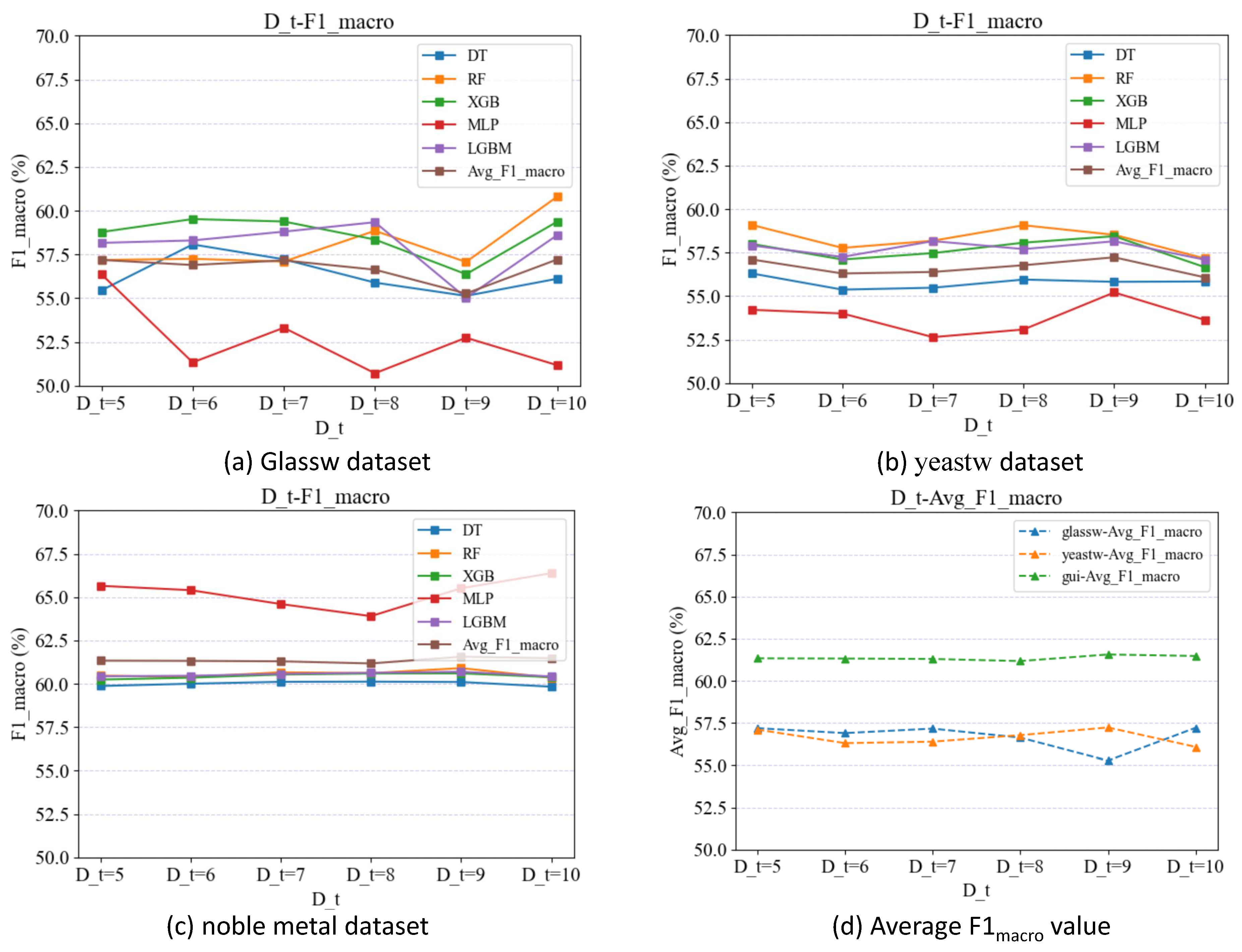
The experimental results are depicted in Figure 8a–c, illustrating the performance of the glassw-generated data, yeastw-generated data, and noble metal-generated data across five classification models. Each figure shows the curve of metric values as $D\_t$ varies. Additionally, Figure 8d displays the average performance of the three generated datasets on classification models, presenting the average curve of metric values from the five classification models for different values of $D\_t$.

Figure 8. Variation curve of D_t with different values.

The experimental results indicate that when $D\_t$ = 7, the performance of the three generated datasets in the classification models stabilizes, characterized by a small range of variation in both $F{1}_{macro}$ values and average $F{1}_{macro}$ values. This suggests that training the generator once and the discriminator seven times achieves a balanced state in terms of data generation capability. However, from Figure 8d, it is evident that starting from $D\_t$ = 8, the performance of the generated data on the classification models begins to fluctuate significantly, indicating larger changes in $F{1}_{macro}$ values. This instability suggests that the model’s data generation capability is no longer stable and that the discriminator may be becoming over-trained, leading to potential overfitting. These findings underscore the importance of moderate training for the discriminator in WAGAN, avoiding both excessive and insufficient training to maintain optimal model performance.

In summary, the training parameters of the WAGAN model are set to $Epoch$ = 10 and $D\_t$ = 7. This setup effectively addresses the issues of unstable training in the original GAN and non-convergence of loss values.

5.3. Bottleneck of the WAGAN Model’s Data Scale

In the parameter-tuning experiment, the influence of the discriminator’s training on the generator is verified by generating data during the generator’s training, ensuring the volume of generated data matches the generator’s training iterations. Initially, the data generated by WAGAN exhibits poor quality due to insufficient diversity information, resulting in generally low classification model performance. To improve the quality of generated data, the trained WAGAN model is employed. However, the quality of the sample set constructed using this method fluctuates, exhibiting instability. This inconsistency arises because while WAGAN can control the category of generated data, it struggles to manage the volume of information contained within, affecting its contribution to the classification model. Moreover, WAGAN may produce duplicate samples, further diminishing sample-set quality. Consequently, this section investigates the data-size bottleneck of WAGAN-generated data, aiming to determine the ideal dataset size with comprehensive information. This investigation serves as the foundation for the sampling experiments detailed in Section 5. Therefore, the primary objective of this experiment is to assess the size of the generated dataset under optimal parameters.

In this experiment, approximately 50% of the original dataset is used for iterative differences in the generation scale, resulting in the generation of 20 batches of samples. The parameters for the generation of iterations across the three datasets are detailed in Table 5. To mitigate the impact of duplicated data on the classification model, the maximum generation threshold is set based on the largest permissible size after removing duplicate samples from the generated dataset. Additionally, equal generation quantities per class are maintained to address any imbalances within the dataset.

Table 5. Dataset generation iteration parameters.

Dataset	Raw Data Size	Generated Batch	Iteration Difference	Maximum Generated Size
glassw	214	20	99	1980
yeastw	1484	20	736	12,800
noble metal	5525	20	2760	55,200

Subsequently, 70% of the original dataset is designated as the training set ($T_{train}$) and utilized to train the classification model ($M_1$), while the remaining 30% serves as the test set ($T_{test}$) for validation purposes. Concurrently, the classification model ($M_2$) is trained using the generated data ($T_{gen}$) post duplicate removal, and the $F{1}_{macro}$ values of models $M_1$ and $M_2$ are evaluated against the test set ($T_{test}$).

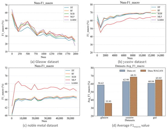
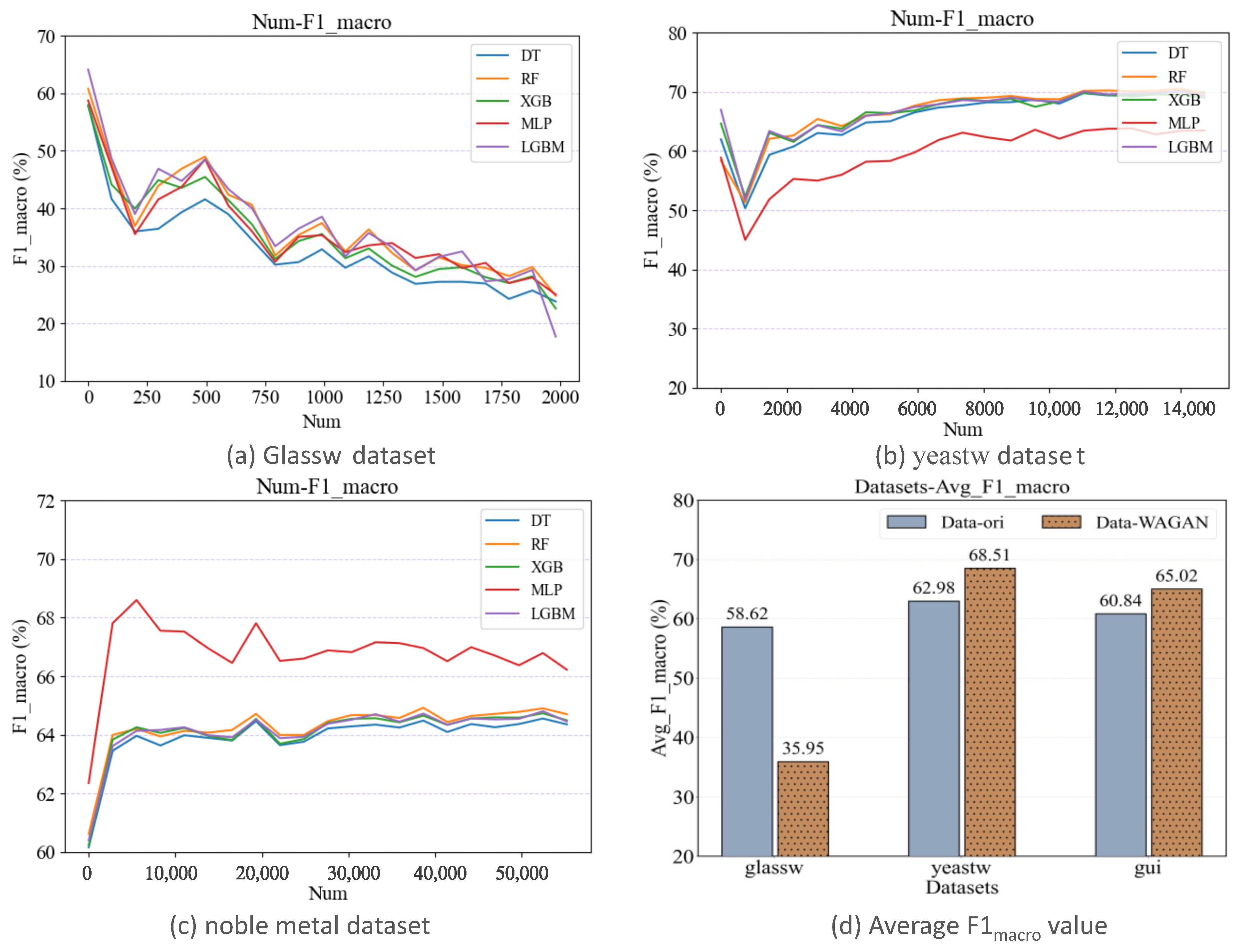
Finally, the aforementioned experiments are conducted on three datasets using five classification models, the results of which are presented in Figure 9. Figure 9a–c illustrate the performance of glassw-generated data, yeastw-generated data, and noble metal-generated data, respectively, across five classification models as the generated scale ($Num$) increases, depicting the curves of $F{1}_{macro}$ values. Figure 9d displays the average performance of both the original data and the generated data at the scale bottleneck on the classification models, showing the histogram of average ($F{1}_{macro}$) values from the five classification models.

Figure 9. $F{1}_{macro}$ value-change curve for the generated data scale.

(1) Analysis of experimental results in Figure 9a: Initially, the glassw dataset has a small number of samples, with some data volumes in the single digits, causing a significant influence of generated noise data on the overall model performance and resulting in a downward trend as the generated data scale increases. However, around a generation scale of 792, the decline in the classification model’s $F{1}_{macro}$ values slows down. This indicates a relative balance between sample data and noise data, with the most comprehensive data information present, represents a data-scale bottleneck. Subsequently, noise data progressively dominate, leading to overfitting and, consequently, severely impacting performance on the test set.

(2) Analysis of experimental results in Figure 9b,c: The yeastw dataset and noble metal dataset both exhibit an overall upward trend as the generation scale increases, indicating increased model performance. However, the generated data may include some noise, initially impacting smaller datasets differently. The yeastw dataset initially shows a slight downward trend due to the influence of noise data, whereas the noble metal dataset shows a consistent upward trend. As the generated data sizes reach 11,776 and 30,360 for the yeastw dataset and noble metal dataset, respectively, they reach a bottleneck in data size. At this point, with further increases in generation scale, the information contained in the generated dataset becomes more comprehensive, and the model’s $F{1}_{macro}$ values no longer show an upward trend but stabilize. To this point, the data volume at the bottleneck for the three datasets is approximately 4.7 times, 7.1 times, and 5.4 times that of the original dataset, respectively.

(3) Analysis of experimental results in Figure 9d: The average $F{1}_{macro}$ values of the generated data on the yeastw dataset and noble metal dataset improve the original precision by 8.7% and 6.8%, respectively. However, the average $F{1}_{macro}$ values on the glassw dataset show a declining trend, which is attributed to the significant influence of noise data on single-class datasets with smaller sample sizes. Nonetheless, this experiment primarily focuses on identifying the scale bottleneck where the generated data contain complete information. Consequently, when the performance of the generated data stabilizes on the classification model, the glassw dataset also reaches its scale bottleneck.

Table 6 presents the average $F{1}_{macro}$ value generation scale bottleneck points of the five classification models and the corresponding dataset sizes. In the table, $Num$ denotes the size of the generated dataset at the scale bottleneck, $AvFm$ represents the precision of the classification model trained using the original dataset, and $AvFm$-w indicates the precision of the classification model trained using the dataset at the scale bottleneck.

Table 6. Generated data-scale bottleneck precision.

Algorithm	Glassw Dataset			Yeastw Dataset			Noble Metal Dataset
	AvFm	AvFm-w	Num	AvFm	AvFm-w	Num	AvFm	AvFm-w	Num
WAGAN	58.62%	35.95%	792	62.98%	68.51%	11,776	60.84%	65.02%	30,360

In conclusion, the sample set constructed by the WAGAN method exhibits varying quality, demonstrating instability. Therefore, this study investigates the scale bottleneck for the generation of data with complete information, using it as the foundational dataset for the subsequent SACS circular sampling method. Furthermore, recognizing that different datasets have distinct scale bottlenecks, this paper incorporates a batch generation functionality into the data generation module, allowing users to customize the generation scale according to their specific needs.

5.4. Related Experiments on the SACS Cyclic Sampling Method

Based on the above experiment, it can be concluded that the generated sample set contains complete data information at the scale bottleneck. At this point, the $F{1}_{macro}$ value of the generated data on the classification model tends to stabilize, but the labels of the generated data are not completely reliable, and a lot of noisy data is generated during the data generation process, which increases the burden on the model, prolongs the training time, and impacts the overall precision of the model to a certain extent. Therefore, this paper aims to construct a higher-quality sample set while ensuring that diverse information is not overlooked.

This experiment involves direct sampling of minority data from the original dataset and cyclically selecting minority data based on their respective categories. Initially, the base dataset for the sampling experiment is established as the dataset generated at the bottleneck of the WAGAN scale. Next, the batch-sampling quantity (n) is defined for the active query strategy (GLUS), representing the difference between the maximum data quantity among sample sets and the current class quantity. Subsequently, the sampling set is constructed to ensure consistency between the classification of pseudo-labels and the generation of pseudo-labels. Finally, following the update strategy of the SAF, the batch-sampling size (m) is determined, along with the threshold size (k), which denotes the final number of current classes after sampling.

Based on the test set ($T_{test}$) divided at the aforementioned scale bottleneck, experimental verification is conducted using five classification models. The results are presented in Table 7. $AvFm$-s denotes the average $F{1}_{macro}$ values across five classification models when the final sample set is balanced. The m parameter signifies the update policy of the SAF, while k and n denote the amount of data per single class and the total amount of data in the final sample set, respectively.

Table 7. Sampling data precision.

Algorithm	Glassw Dataset				Yeastw Dataset				Noble Metal Dataset
	AvFm-s	m	k	n	AvFm-s	m	k	n	AvFm-s	m	k	n
SACS	65.41%	10	76	684	73.14%	40	463	3704	72.78%	30	316	14,536

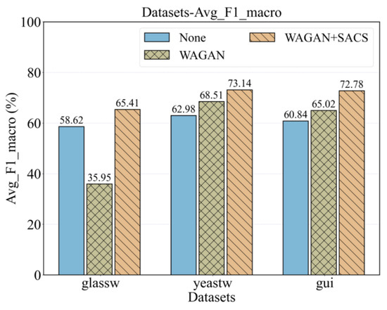
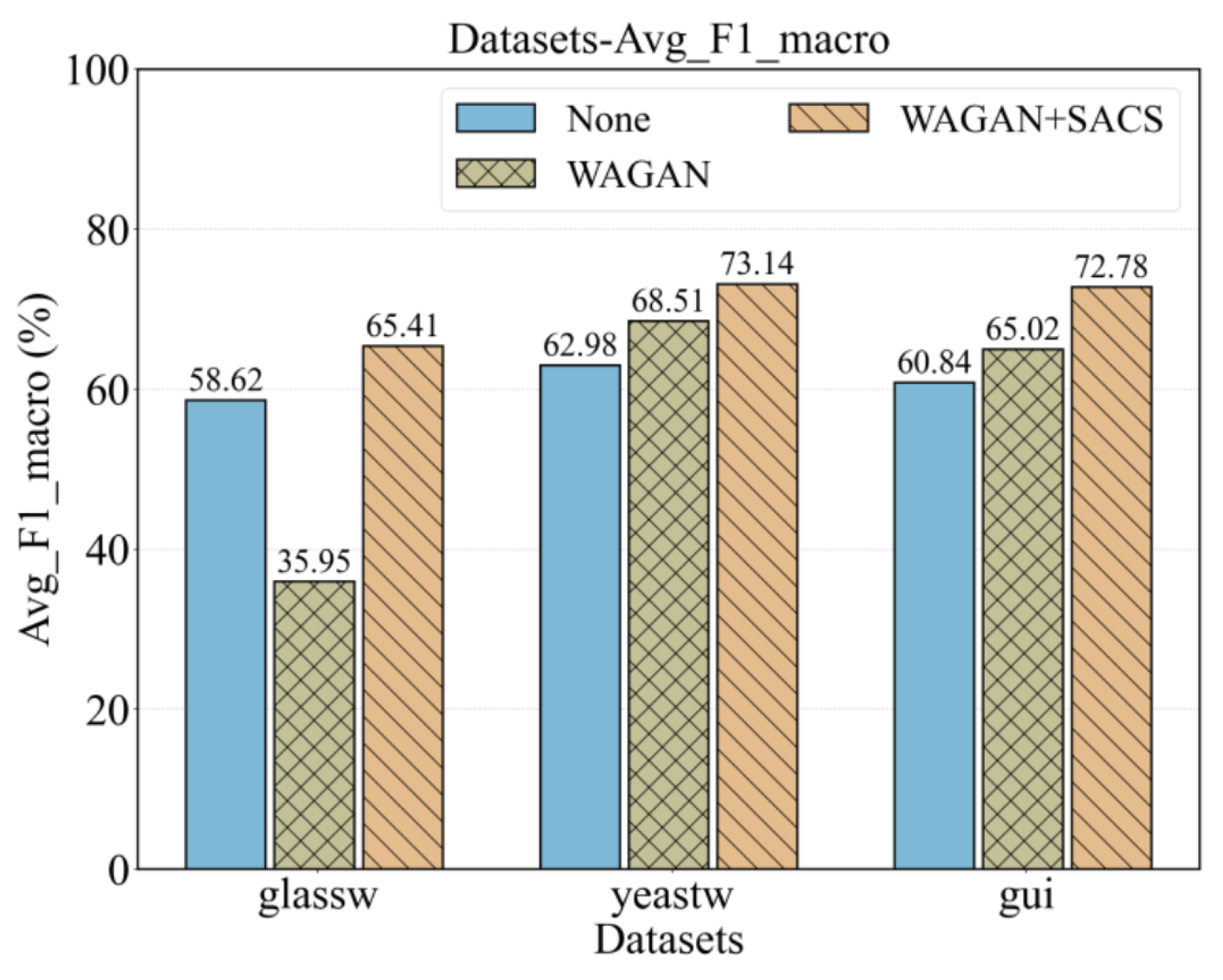
The experimental results demonstrate that the average $F{1}_{macro}$ values of the sample set constructed after sampling in the classification model are improved compared to the dataset generated at the bottleneck of the WAGAN scale. This confirms the presence of noise data in the initial dataset generation phase, which impacts the overall model precision. Moreover, compared to the average $F{1}_{macro}$ values of the classification model presented in Figure 8d, the sampled average $F{1}_{macro}$ values achieve unprecedented heights, further indicating that the WAGAN model generates noise data during the data generation process, thereby affecting the model’s classification ability. The average improvement in $F{1}_{macro}$ values achieved by the SACS cyclic sampling algorithm is depicted in Figure 10. None denotes the precision of the classification model trained using the original dataset, WAGAN represents the precision using the scale bottleneck dataset, and WAGAN+SACS represents the precision using the final dataset.

Figure 10. Average $F{1}_{macro}$ value bar chart.

In summary, although the average $F{1}_{macro}$ value of the WAGAN data generation method decreased to 0.3595 on the glassw dataset, it increases by 8.7% and 6.8% on the yeastw and noble metal datasets, respectively. This proves that noise significantly impacts smaller datasets. The WAGAN+SACS method mitigates this issue, resulting in improvements of 11.5%, 16.1%, and 19.6% on the three datasets. This fully demonstrates that the data enhancement method can eliminate the influence of the unstable quality of the sample set generated by WAGAN, reducing the burden on the model caused by an excessive training set while improving model precision. Additionally, this method not only addresses the issues of small capacity in structured data and uneven category distribution but also constructs a higher-quality sample set.

5.5. Comparative Data Augmentation Experiment

This paper focuses on addressing the issues of small capacity in structured data and uneven category distribution. To validate the proposed data enhancement method, i.e., WAGAN+SACS, this experiment compares it with existing data enhancement methods, specifically balanced dataset enhancement methods, including the Random OverSampling (ROS) algorithm, the Synthetic Minority Over-sampling Technique (SMOTE), the Borderline-SMOTE algorithm, the Adaptive Synthetic (ADASYN) algorithm, and the CGAN data synthesis method.

The main task of this experiment is to perform data enhancement experiments on five algorithms, aiming to verify the effectiveness of this method through comparative experiments. To better conduct the comparative experiment, the test set ($T_{test}$) for the classification model remains the same as the test set ($T_{test}$) of the three datasets used in the previous section. Then, experiments are carried out on five classification models, and their average $F{1}_{macro}$ values are calculated. The experimental results are shown in Table 8. AvFm represents the average $F{1}_{macro}$ value of the classification model, and AvFm-c represents the amplitude of the average $F{1}_{macro}$ value change after applying the data enhancement algorithm.

Table 8. Comparative experimental precision table.

Algorithm	Glassw		Yeastw		Noble Metal
	AvFm	AvFm-c	AvFm	AvFm-c	AvFm	AvFm-c
None	58.62	0.00	62.98	0.00	60.84	0.00
ROS	35.05	↓23.57	32.27	↓30.71	23.53	↓37.31
SMOTE	60.32	↑1.70	68.29	↑5.31	59.85	↓0.99
B-SMOTE	64.58	↑5.96	73.02	↑10.04	68.78	↑7.94
ADASYN	64.66	↑6.04	69.64	↑6.66	65.67	↑4.83
CGAN	63.61	↑4.99	71.78	↑8.80	69.38	↑8.54
Proposed method	65.40	↑6.78	73.14	↑10.16	72.78	↑11.94

The experimental results show that the average $F{1}_{macro}$ value of ROS on the glassw dataset, yeastw dataset, and noble metal dataset is lower than the average $F{1}_{macro}$ value of the original dataset. This is due to the simple replication of a few samples when the random oversampling algorithm enhances the dataset, which eventually leads to overfitting. Both the Borderline-SMOTE algorithm and the ADASYN algorithm perform better than the SMOTE algorithm on the classification model, proving that the SMOTE algorithm blurs the boundary during interpolation synthesis, leading to misclassification by the model and ultimately reducing its recognition precision. The performance of the CGAN algorithm on the yeastw dataset and the noble metal dataset is better than on the glassw dataset because the glassw dataset is small in scale, and the generated noise data significantly impact it during the balancing process. A single data generation method cannot avoid this situation. Meanwhile, the WAGAN+SACS data enhancement method proposed in this paper achieves a higher average $F{1}_{macro}$ value than the other five algorithms on the classification model, demonstrating that this method not only addresses the issues of small capacity and unbalanced categories in structured data but also constructs a higher-quality sample set.

6. Conclusions and Future Work

To address the problem of small capacity of structured data and uneven distribution among tag classes, this paper proposes a structured data generation method called WAGAN. This method not only enriches the diversified information of small-sample structured data but also effectively avoids the disadvantages of mode collapse and gradient vanishing in the training of the original GAN. To enhance the reliability of generated data pseudo-labels and build a higher-quality sample set, this paper proposes a cyclic sampling method based on semi-supervised active learning, building upon the WAGAN data generation method. This method comprises the following two parts: the SAF and the spatial overlap-based uncertainty sampling strategy. This method not only weakens the impact of noisy data on the overall precision of the classification model but also enhances the reliability of generated pseudo-labels and constructs a higher-quality sample set. Experimental results show that the sample set constructed by the WAGAN+SACS data enhancement method outperforms other data enhancement methods in the classification model. Compared with the original data, the average $F{1}_{macro}$ values of the five classification models on three datasets are improved by 11.5%, 16.1%, and 19.6%, respectively, verifying the effectiveness of the proposed method.

Significant development is expected in many research fields in the future. (1) Related to problems of data generation, the WAGAN generation method proposed in this paper is oriented towards structured data, so the neural network structures of the generator and discriminator adopt a more portable, full connection. In the future, data generation methods can be optimized in more detail by introducing other neural network structures for different fields. Additionally, the WAGAN model focuses on providing a data basis for sampling methods and is not compared with other existing structured data generation models. Future research can further study and optimize the WAGAN model to enhance its data generation capability. (2) With respect to data sampling-related problems, the SACS cyclic sampling method proposed in this paper focuses on enhancing the label reliability of WAGAN-generated data and constructing a high-quality training sample set, which are strongly correlated. In the future, the data sampling module can be split for more in-depth research and used independently for other small-sample learning tasks to reduce the model’s dependence on data. (3) In terms of optimization of classification models, this paper verifies the final sample set using five common classification models in multi-classification tasks to prove the universality of the sample set in classification models. In the future, classification models can be optimized according to specific learning tasks to better improve the precision and generalization ability of the model.

References

- Cai, Z.; Ma, W.; Wang, X.; Wang, H.; Feng, Z. The Performance Analysis of Time Series Data Augmentation Technology for Small Sample Communication Device Recognition. IEEE Trans. Reliab. 2023, 72, 574–585. [Google Scholar] [CrossRef] [Scilit]
- Kaur, H.; Pannu, H.S.; Malhi, A.K. A systematic review on imbalanced data challenges in machine learning: Applications and solutions. ACM Comput. Surv. 2019, 52, 1–36. [Google Scholar] [CrossRef] [Scilit]
- Krizhevsky, A.; Sutskever, I.; Hinton, G.E. Imagenet classification with deep convolutional neural networks. Commun. ACM 2017, 60, 84–90. [Google Scholar] [CrossRef] [Scilit]
- Wei, W.; Deng, D.; Zeng, L.; Zhang, C. Real-time implementation of fabric defect detection based on variational automatic encoder with structure similarity. J. Real Time Image Process. 2021, 18, 807–823. [Google Scholar] [CrossRef] [Scilit]
- Goodfellow, I.; Pouget-Abadie, J.; Mirza, M.; Xu, B.; Warde-Farley, D.; Ozair, S.; Courville, A.; Bengio, Y. Generative adversarial nets. Adv. Neural Inf. Process. Syst. 2014, 27, 2672–2680. [Google Scholar]
- Van, E.J.E.; Hoos, H.H. A survey on semi-supervised learning. Mach. Learn. 2020, 109, 373–440. [Google Scholar]
- Cohn, D.A.; Ghahramani, Z.; Jordan, M.I. Active learning with statistical models. J. Artif. Intell. Res. 1996, 4, 129–145. [Google Scholar] [CrossRef] [Scilit]
- Tay, Y.C.; Dai, B.T.; Wang, D.T.; Sun, E.Y.; Lin, Y.; Lin, Y. UpSizeR: Synthetically scaling an empirical relational database. Inf. Syst. 2013, 38, 1168–1183. [Google Scholar] [CrossRef] [Scilit]
- Zhu, L.; Zhang, Z.; Song, D.; Chen, B. Analysis of traffic accident causes based on data augmentation and ensemble learning with high-dimensional small-sample data. Expert Syst. Appl. 2024, 237, 121782. [Google Scholar] [CrossRef] [Scilit]
- Song, X.; He, Y.; Li, X.; Zhu, Q.X.; Xu, Y. Novel virtual sample generation method based on data augmentation and weighted interpolation for soft sensing with small data. Expert Syst. Appl. 2023, 225, 120085. [Google Scholar] [CrossRef] [Scilit]
- Jiang, W.; Ling, L.; Zhang, D.; Lin, R.; Zeng, L. A Time Series Forecasting Model Selection Framework using CNN and Data Augmentation for Small Sample Data. Neural Process. Lett. 2023, 55, 5783–5810. [Google Scholar] [CrossRef] [Scilit]
- Zhang, Y.; Yang, Q. A survey on multi-task learning. IEEE Trans. Knowl. Data Eng. 2022, 34, 5586–5609. [Google Scholar] [CrossRef] [Scilit]
- Sun, Y.; Ding, S.; Zhang, Z.; Jia, W. An improved grid search algorithm to optimize SVR for prediction. Soft Comput. 2021, 25, 5633–5644. [Google Scholar] [CrossRef] [Scilit]
- Bergstra, J.; Bengio, Y. Random search for hyper-parameter optimization. J. Mach. Learn. Res. 2012, 13, 281–305. [Google Scholar]
- Huisman, M.; Van, R.J.N.; Plaat, A. A survey of deep meta-learning. Artif. Intell. Rev. 2021, 54, 4483–4541. [Google Scholar] [CrossRef] [Scilit]
- Pan, S.J.; Yang, Q. A survey on transfer learning. IEEE Trans. Knowl. Data Eng. 2010, 22, 1345–1359. [Google Scholar] [CrossRef] [Scilit]
- Huang, L.; Fan, J.; Zhao, W.; You, Y. A new multi-source Transfer Learning method based on Two-stage Weighted Fusion. Knowl. Based Syst. 2023, 262, 110233. [Google Scholar] [CrossRef] [Scilit]
- Zhang, R.; Zhang, Z.; Wang, D. RFCL: A new under-sampling method of reducing the degree of imbalance and overlap. Pattern Anal. Appl. 2021, 24, 641–654. [Google Scholar] [CrossRef] [Scilit]
- Das, B.; Krishnan, N.C.; Cook, D.J. RACOG and wRACOG: Two Probabilistic Oversampling Techniques. IEEE Trans. Knowl. Data Eng. 2015, 27, 222–234. [Google Scholar] [CrossRef] [Scilit]
- Estabrooks, A.; Jo, T.; Japkowicz, N. A multiple resampling method for learning from imbalanced datasets. Comput. Intell. 2004, 20, 18–36. [Google Scholar] [CrossRef] [Scilit]
- Tsai, C.F.; Lin, W.C.; Hu, Y.H.; Yao, G.T. Under-sampling class imbalanced datasets by combining clustering analysis and instance selection. Inf. Sci. 2019, 477, 47–54. [Google Scholar] [CrossRef] [Scilit]
- Chawla, N.V.; Bowyer, K.W.; Hall, L.O.; Kegelmeyer, W.P. SMOTE: Synthetic minority over-sampling technique. J. Artif. Intell. Res. 2002, 16, 321–357. [Google Scholar] [CrossRef] [Scilit]
- Han, H.; Wang, W.; Mao, B. Borderline-SMOTE: A New Over-Sampling Method in Imbalanced Data Sets Learning. In Proceedings of the International Conference on Intelligent Computing, ICIC, Hefei, China, 23–26 August 2005; pp. 878–887. [Google Scholar]
- He, H.; Bai, Y.; Garcia, E.A.; Li, S. ADASYN: Adaptive synthetic sampling approach for imbalanced learning. In Proceedings of the 2008 IEEE International Joint Conference on Neural Networks (IEEE World Congress on Computational Intelligence), Hong Kong, China, 1–6 June 2008; pp. 1322–1328. [Google Scholar]
- Wang, K.; Gou, C.; Duan, Y.; Lin, Y.; Zheng, X.; Wang, F.Y. Generative adversarial networks: Introduction and outlook. IEEE CAA J. Autom. Sin. 2017, 4, 588–598. [Google Scholar] [CrossRef] [Scilit]
- Yu, H.; Wang, Q.F.; Shi, J.Y. Data Augmentation Generated by Generative Adversarial Network for Small Sample Datasets Clustering. Neural Process. Lett. 2023, 55, 8365–8384. [Google Scholar] [CrossRef] [Scilit]
- Biau, G.; Sangnier, M.; Tanielian, U. Some theoretical insights into Wasserstein GANs. J. Mach. Learn. Res. 2021, 22, 1–45. [Google Scholar]
- Jin, Q.; Lin, R.; Yang, F. E-WACGAN: Enhanced generative model of signaling data based on WGAN-GP and ACGAN. IEEE Syst. J. 2020, 14, 3289–3300. [Google Scholar] [CrossRef] [Scilit]
- Wang, Y.; Yu, B.; Wang, L.; Zu, C.; Lalush, D.S.; Lin, W.; Wu, X.; Zhou, J.; Shen, D.; Zhou, L. 3D conditional generative adversarial networks for high-quality PET image estimation at low dose. Neuroimage 2018, 174, 550–562. [Google Scholar] [CrossRef] [Scilit]
- Kang, M.; Shim, W.; Cho, M.; Park, J. Rebooting acgan: Auxiliary classifier gans with stable training. Adv. Neural Inf. Process. Syst. 2021, 34, 23505–23518. [Google Scholar]
- Li, J.; Zhu, Q.; Wu, Q. A self-training method based on density peaks and an extended parameter-free local noise filter for k nearest neighbor. Knowl. Based Syst. 2019, 184, 104895. [Google Scholar] [CrossRef] [Scilit]
- Peng, J.; Estrada, G.; Pedersoli, M.; Desrosiers, C. Deep co-training for semi-supervised image segmentation. Pattern Recognit. 2020, 107, 107269. [Google Scholar] [CrossRef] [Scilit]
- Tanha, J.; Van, S.M.; Afsarmanesh, H. Semi-supervised self-training for decision tree classifiers. Int. J. Mach. Learn. Cybern. 2017, 8, 355–370. [Google Scholar] [CrossRef] [Scilit]
- Chong, Y.; Ding, Y.; Yan, Q.; Pan, S. Graph-based semi-supervised learning: A review. Neurocomputing 2020, 408, 216–230. [Google Scholar] [CrossRef] [Scilit]
- Agrawal, A.; Tripathi, S.; Vardhan, M. Active learning approach using a modified least confidence sampling strategy for named entity recognition. Prog. Artif. Intell. 2021, 10, 113–128. [Google Scholar] [CrossRef] [Scilit]
- Ren, P.; Xiao, Y.; Chang, X.; Huang, P.Y.; Li, Z.; Gupta, B.B.; Chen, X.; Wang, X. A survey of deep active learning. ACM Comput. Surv. 2022, 54, 1–40. [Google Scholar] [CrossRef] [Scilit]
- Xu, H.; Li, L.; Guo, P. Semi-supervised active learning algorithm for SVMs based on QBC and tri-training. J. Ambient Intell. Humaniz. Comput. 2021, 12, 8809–8822. [Google Scholar] [CrossRef] [Scilit]
- Tom, F. CNN-LSTM-Based Fault Diagnosis and Adaptive Multichannel Fusion Calibration of Filament Current Sensor for Mass Spectrometer. IEEE Sens. J. 2024, 24, 2255–2269. [Google Scholar]
Disclaimer/Publisher’s Note: The statements, opinions and data contained in all publications are solely those of the individual author(s) and contributor(s) and not of MDPI and/or the editor(s). MDPI and/or the editor(s) disclaim responsibility for any injury to people or property resulting from any ideas, methods, instructions or products referred to in the content. |
© 2024 by the authors. Licensee MDPI, Basel, Switzerland. This article is an open access article distributed under the terms and conditions of the Creative Commons Attribution (CC BY) license (https://creativecommons.org/licenses/by/4.0/).