Adaptive Iterative Learning Constrained Control for Linear Motor-Driven Gantry Stage with Fault-Tolerant Non-Repetitive Trajectory Tracking

Abstract

This article introduces an adaptive fault-tolerant control method for non-repetitive trajectory tracking of linear motor-driven gantry platforms under state constraints. It provides a comprehensive solution to real-world issues involving state constraints and actuator failures in gantry platforms, alleviating the challenges associated with precise modeling. Through the integration of iterative learning and backstepping cooperative design, this method achieves system stability without requiring a priori knowledge of system dynamic models or parameters. Leveraging a barrier composite energy function, the proposed controller can effectively regulate the stability of the controlled system, even when operating under state constraints. Instability issues caused by actuator failures are properly addressed, thereby enhancing controller robustness. The design of a trajectory correction function further extends applicability. Experimental validation on a linear motor-driven gantry platform serves as empirical evidence of the effectiveness of the proposed method.

1. Introduction

In recent years, with the ongoing advancement of modern industry towards intelligence and efficiency [1,2,3], linear motor-driven gantry stages (LMDGSs) have found widespread application [4,5] in the high-speed, high-precision intelligent equipment industry, such as surface mount technology (SMT), mechanical machining centers, and lithography machines, due to its rapid and precise positioning capabilities [6,7]. Consequently, a plethora of complex control issues have emerged [8,9], and solutions to these problems are still being actively researched and explored [10,11].

The first challenge addressed in this article pertains to the state constraints of LMDGSs [12,13,14]. In the practical applications of these platforms, it is common practice to impose state constraints on the system to ensure safety and control effectiveness. For instance, due to the limited travel range of LMDGSs, maximum value constraints are placed on the position states of the moving platform to ensure safety [15]. Introducing time-varying dynamic position constraints on the motion segment of LMDGSs aims at achieving the desired tracking error in line with actual motion [16,17,18]. Using the barrier composite energy function and backstepping cooperative design, the controller in [19] can effectively regulate the stable operation of the controlled system, even when the state of the linear motor is constrained.

In addition to dynamic state constraints, actuator faults [20,21,22] also demand attention, as system reliability is of paramount importance for LMDGSs. In practical applications, continuous operation of LMDGSs 24 h a day is common, and under prolonged, uninterrupted, and high-intensity operation, wear and tear gradually accumulates on actuators. Moreover, unforeseen events may cause the permanent degradation of actuator output capabilities. Since these changes are usually challenging to detect and repair promptly, this article also explores solutions to address actuator fault issues [23,24]. By introducing the event-triggered adaptive control law [25], online adaptive adjustments are achieved, enhancing applicability and robustness to actuator faults. Actually, it mitigates the impact of both actuator faults and measurement error parameters [26].

In practical applications of LMDGSs, most scenarios involve extended periods of repetitive tasks. This feature makes iterative learning control (ILC) have a better control effect and lower control complexity than adaptive robust control (ARC) and proportional-integral-differential (PID) [19]. This paper builds on the work of [19] to further improve the iterative learning controller by adding non-repetitive trajectory tracking capabilities and fault-tolerant control. This article aims at applying ILC as the cornerstone for devising a comprehensive solution to the aforementioned issues. Nevertheless, real-world applications inevitably introduce certain non-repetitive constraints, such as obstacle avoidance, which disrupt the repetitive nature of the tasks [27]. In [28], an ILC method is introduced based on an advanced internal model, along with convergence conditions, achieving robust tracking for non-repetitive system tasks. To enhance practicality and broaden the applicability of the control strategy, this article introduces a trajectory correction function to address non-repetitive trajectory challenges.

Considering the circumstances outlined above, this article introduces a non-repetitive trajectory adaptive iterative learning fault-tolerant controller for LMDGSs with state constraints, even in the absence of precise model information. The key contributions of this work are as follows:

• The designed controller achieves the desired tracking precision without requiring precise modeling or precise a priori knowledge of the system;
• By formulating a Barrier Composite Energy Function (BCEF) and integrating it into the controller design, the tracking control challenge associated with a LMDGS subject to state variables constraints is properly addressed;
• By incorporating the contributions of the controller’s output fault term, the designed control scheme can effectively mitigate to a significant extent the adverse effects of actuator failures, ensuring system’s convergence.
• By introducing in the design the desired trajectory correction function, non-repetitive desired trajectories can be effectively tracked while ensuring convergence of the system’s tracking error.

The subsequent sections of this article are structured as follows. In Section 2, the tracking problem for an LMDGS is defined and a simplified plant model is presented. The trajectory correction function is designed in Section 3. Section 4 delves into a comprehensive exploration of the controller design and the BCEF. In Section 5, convergence and finiteness aspects of the proposed ILC tracking scheme are analyzed. Experimental results are presented and discussed in Section 6. Finally, Section 7 presents the concluding remarks and findings of this work.

2. Problem Statement and Preliminaries

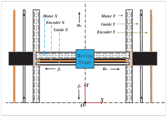
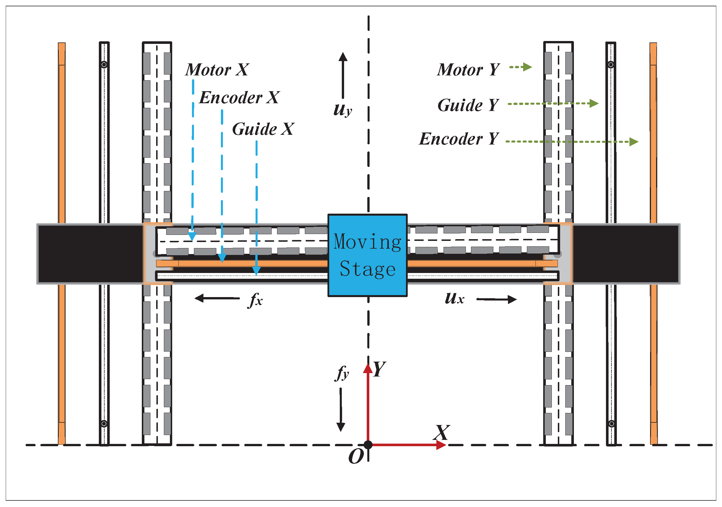
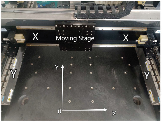
The LMDGS depicted in Figure 1 is a two-dimensional multiple-input-multiple-output-system. This system exhibits parametric and non-parametric uncertainties due to discrepancies between nominal and real values, as well as losses incurred during actual system operation. A simplified continuous time model of the LMDGS can be represented as

$$\begin{array}{cc}\hfill \dot{\mathit{s}}=& \mathit{v},\hfill \\ \hfill \mathit{m}\dot{\mathit{v}}=& \mathit{g}{\mathit{u}}^F-S_f{\mathit{k}}_{\mathit{c}}-{\mathit{k}}_{\mathit{v}}\mathit{v}+{\mathit{d}}_{\mathbf{1}},\hfill \\ \hfill {\mathit{u}}^F=& p\mathit{u}+\varphi ,\hfill \\ \hfill \mathit{y}=& \{\mathit{s},\mathit{v}\},\hfill \end{array}$$

(1)

where $\mathit{m}$ = ${[m_x,m_y]}^T$ denotes the masses of the X and Y axes moving parts, $\mathit{s}$ = ${[s_x\left(t\right),s_y\left(t\right)]}^T$ represents the position of the motion axis, and $\mathit{v}$ = ${[v_x\left(t\right),v_y\left(t\right)]}^T$ is the corresponding velocity. $S_f{\mathit{k}}_{\mathit{c}}\in R^{2\times 1}$ refers to approximate Coulomb friction, where $S_f=S_f\left(\mathit{v}\right)$ is an unknown continuous function. ${\mathit{k}}_{\mathit{v}}\mathit{v}\in R^{2\times 1}$ is the viscous friction. ${\mathit{k}}_{\mathit{c}}$ and ${\mathit{k}}_{\mathit{v}}$ denote friction coefficients. $\mathit{f}=S_f{\mathit{k}}_{\mathit{c}}+{\mathit{k}}_{\mathit{v}}\mathit{v}$ denotes the system’s reverse resistance and ${\mathit{d}}_{\mathbf{1}}(\mathit{s},\mathit{v},t)={[d_x\left(t\right),d_y\left(t\right)]}^T$ represents external disturbances and unknown system dynamics. $\mathit{g}$ = diag$[g_x\left(t\right),g_y\left(t\right)]$ is the gain function, which is not fully known. The controller input is $\mathit{u}=\mathit{u}\left(t\right)\in R^{2\times 1}$. When affected by actuator failure, the actual input to the controlled plant is ${\mathit{u}}^F$. $p=\mathrm{diag}[p_1,p_2]\in R^{2\times 2}$ represents multiplicative actuator fault and $\varphi \in R^{2\times 1}$ denotes additive actuator fault. Both actuator faults can vary with time and iteration, whereas $0<p_1,p_2\le 1$. $\mathit{y}$ is the system output. To facilitate subsequent operations, transform system (1) into the following by introducing new variables: ${\mathit{X}}_1=\mathit{s}$, ${\mathit{X}}_2=\mathit{v}$, $\mathit{X}\triangleq {\{{\mathit{X}}_1^T,{\mathit{X}}_2^T\}}^T$, $G=g$, ${\mathrm{\Phi }}^{T}F=-S_f{\mathit{k}}_{\mathit{c}}/\mathit{m}$, and $d=(d_1(\mathit{X},t)-{\mathit{k}}_{\mathit{v}}\mathit{v})/\mathit{m}$.

$$\begin{array}{cc}\hfill {\mathit{X}}_1& ={\mathit{X}}_2,\hfill \\ \hfill {\dot{\mathit{X}}}_2& ={\mathrm{\Phi }}^{T}F+d+G{u}^F,\hfill \\ \hfill {\mathit{u}}^F& =p\mathit{u}+\varphi ,\hfill \\ \hfill \mathit{y}& =\{{\mathit{X}}_1,{\mathit{X}}_2\}.\hfill \end{array}$$

(2)

Figure 1. LMDGS structure.

Then, the system (2) is transformed into the corresponding n-th iterative form as follows:

$$\begin{array}{cc}\hfill {\mathit{X}}_{1,n}& ={\mathit{X}}_{2,n},\hfill \\ \hfill {\dot{\mathit{X}}}_{2,n}& ={\mathrm{\Phi }}^T{F}_n+d_n+G_n{u}_n^F,\hfill \\ \hfill {\mathit{u}}_n^F& =p_n{\mathit{u}}_n+{\varphi }_n,\hfill \\ \hfill \mathit{y}& =\{{\mathit{X}}_{1,n},{\mathit{X}}_{2,n}\}.\hfill \end{array}$$

(3)

System states ${\mathit{X}}_{1,n}={\mathit{X}}_{1,n}\left(t\right)\in R^{2\times 1}$ and ${\mathit{X}}_{2,n}={\mathit{X}}_{2,n}\left(t\right)\in R^{2\times 1}$ represent the state of the system at the n-th iteration, and $n\in Z_{+}$. $\mathit{X}\triangleq {\{{\mathit{X}}_1^T,{\mathit{X}}_2^T\}}^T$, ${\mathit{X}}_n\triangleq {\{{\mathit{X}}_{1,n}^T,{\mathit{X}}_{2,n}^T\}}^T$, $t\in [0,\breve{T}]$, $\breve{T}\in R^{+}$ signifies the time taken for each system iteration. The unmodeled dynamics and unknown external disturbances $d_n=d_n\left(t\right)\in R^{2\times 1}$ at the n-th iteration. ${\mathrm{\Phi }}^T{F}_n$ refers to the parametric uncertainty, the unknown iteration invariant is given by $\mathrm{\Phi }=\mathrm{\Phi }\left(t\right)\in R^{2\times 2}$, and $F_n=F({\mathit{X}}_n,t)\in R^{2\times 1}$ is a known state-dependent nonlinear function at the n-th iteration. In addition, $G_n=G_n\left(t\right)\in R^{2\times 2}$ is the unknown control input gain function at the n-th iteration. The controller input is ${\mathit{u}}_n=u_n\left(t\right)\in R^{2\times 1}$ at the n-th iteration. When affected by actuator failure, the actual input to the controlled plant is ${\mathit{u}}_n^F$ at the n-th iteration. $p_n=p_n\left(t\right)=diag[p_{n,1}\left(t\right),p_{n,2}\left(t\right)]\in R^{2\times 2}$ represents multiplicative actuator fault and ${\varphi }_n\in R^{2\times 1}$ denotes additive actuator fault at the n-th iteration. Both actuator faults can vary with time and iteration, whereas $0<p_{n,1},p_{n,2}\le 1$.

ILC is a method in control systems where a controller is refined through repetition. It is designed for processes that repeat in cycles, allowing the controller to learn from previous cycles to improve performance in subsequent ones [29]. ILC involves tracking error update control signals based on earlier iterations, continuously improving the response and stability of the system through n iterations of updates. The simple mathematical equation of the P-type iterative learning controller is as follows:

$$\begin{array}{c}\hfill {\mathit{u}}_n={\mathit{u}}_{n-1}+K_p(X_{1,n}-X_{1r,n}),\end{array}$$

(4)

where $K_p$ is the learning rate and $X_{1r,n}$ refers to the system reference position state at the n-th iteration. For the convenience of further discussion, the following assumptions are considered:

Assumption 1.

Generalized control input gain function $G_{u,n}=\left(((G_n{p}_n+{\left(G_n{p}_n\right)}^T)/2)\right)$ is positive definite and bounded.

Remark 1.

This assumption is very practical in many engineering systems. In real engineering systems, the control input gain is generally positive and bounded, owing to the limited power of the actuators themselves. This condition is essential for maintaining consistency of control direction during operation. Note, that complete information regarding the control input gain function is usually not available. The existence of specific upper or lower bounds for the gain function is unknown. Thus, $0<\underline{b}{I}_m\le G_{u,n}$, where $\underline{b}$ is unknown.

Assumption 2.

Regarding control input gain, actuator fault, and unmodeled dynamics, $\left|\right|d_n+G_n{\varphi }_n\left|\right|$ has an unknown upper bound $\overline{d}>0$.

Remark 2.

In real-world engineering applications, disturbances during system operation are typically bounded. These disturbances can disrupt system stability but are not typically large enough to cause system shutdown directly. Assumption 2 can be readily extended to encompass constraints with Lipschitz-like characteristics.

Assumption 3.

${\mathrm{\Phi }}_n$ has an unknown bound $\overline{\theta }$, $0<\left|\right|{\mathrm{\Phi }}_n\left|\right|\le \overline{\theta }$.

Remark 3.

${\mathrm{\Phi }}_n$ represents the system’s parameter uncertainty. In real engineering scenarios, the parameters of physical systems are generally limited and tend to change slowly. In common practical scenarios, ${\mathrm{\Phi }}_n$ remains independent of the iteration index n. However, in this article, the possibility of ${\mathrm{\Phi }}_n$ varying with iterations is considered, thus expanding the applicability of the proposed strategy.

Lemma 1

(see [30]). For any $ϵ>0$ and $z\in R$, it can be obtained that $0\le \left|z\right|-ztanh\left(\frac{z}{ϵ}\right)\le k_lϵ,k_l=0.2785$.

Lemma 2

(see [31]). For a convergent sequence $ϵ=q/k^l$, where $k\in Z_{+},q\in R$, and $l\in Z_{+}$, and $q>0,l>1$, one has ${lim}_{k\to \infty }{\sum }_{j=1}^k{ϵ}_j\le 2q$.

3. Modification of Reference Trajectories

In this article, reference trajectories $X_{1r,n}$ and $X_{2r,n}$ can vary in different iterations. Hence, the system’s initial states can also vary between iterations. That is, the system’s initial state tracking errors are probably not zero, and even vary in each iteration. Therefore, it is impossible for system states to track the desired trajectories well over the entire time $[0,\breve{T}]$ of every iteration. In response, a short initial time interval $[0,{\breve{T}}_1]$ is ignored to ensure good tracking for the rest of the time $[{\breve{T}}_1,\breve{T}]$. Therefore, a new reference trajectory modified method for ILC is proposed in this paper, as follows:

$$\begin{array}{c}\hfill X_{1d,n}\left(t\right)=X_{1r,n}\left(t\right)-\sum _{j=1}^2{\omega }_j\left(t\right)(X_{jr,n}\left(0\right)-X_{j,n}\left(0\right)),\end{array}$$

(5)

and, from the derivative definition,

$$\begin{array}{cc}\hfill X_{2d,n}\left(t\right)& ={\dot{X}}_{1d,n}\left(t\right)\hfill \\ \hfill & ={\dot{X}}_{1r,n}\left(t\right)-\sum _{j=1}^2{\dot{\omega }}_j\left(t\right)(X_{jr,n}\left(0\right)-X_{j,n}\left(0\right))\hfill \\ \hfill & =X_{2r,n}\left(t\right)-\sum _{j=1}^2{\dot{\omega }}_j\left(t\right)(X_{jr,n}\left(0\right)-X_{j,n}\left(0\right)),\hfill \end{array}$$

(6)

where $X_{1d,n}\left(t\right)$ and $X_{2d,n}\left(t\right)$ are the modified desired reference trajectories. ${\omega }_j\left(t\right)\in R,j=1,2$ are “trajectory modifier functions” satisfying the following properties:

(1)

${\omega }_j\left(t\right),j=1,2,$ are 2nd order differentiable;

(2)

${\omega }_j\left(t\right),j=1,2,$ are uniformly bounded over $[0,\breve{T}]$;

(3)

${\omega }_j^{j-1}\left(t\right)=1,j=1,2,$ whereas ${\omega }_j^i\left(t\right)=0,i=0,1,2,i\le j,i\ne j-1$, where ${\omega }_j^i\left(t\right)$ representes the ith order time derivative;

(4)

${\omega }_j^i\left(t\right)=1,j=1,2,i=0,1,2$, over $t\in [{\breve{T}}_1,\breve{T}]$, where $0<{\breve{T}}_1<\breve{T}$.

The example used in this paper is as follows:

$$\begin{array}{c}\hfill {\omega }_j\left(t\right)=\left\{\begin{array}{cc}\frac{t^{j-1}}{(j-1)!}{cos}^3\left(\frac{\pi }{2}{sin}^3\left(\frac{\pi t^2}{2{\breve{T}}_1^2}\right)\right),\hfill & t\in [0,{\breve{T}}_1)\hfill \\ 0,\hfill & t\in [{\breve{T}}_1,\breve{T}],\hfill \end{array}\right.\end{array}$$

(7)

where $j=1,2$, and ! represents a factorial, namely $j!=j(j-1)\cdots 1$.

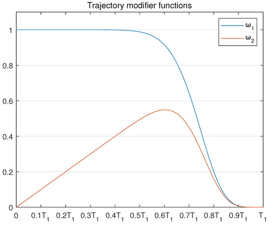
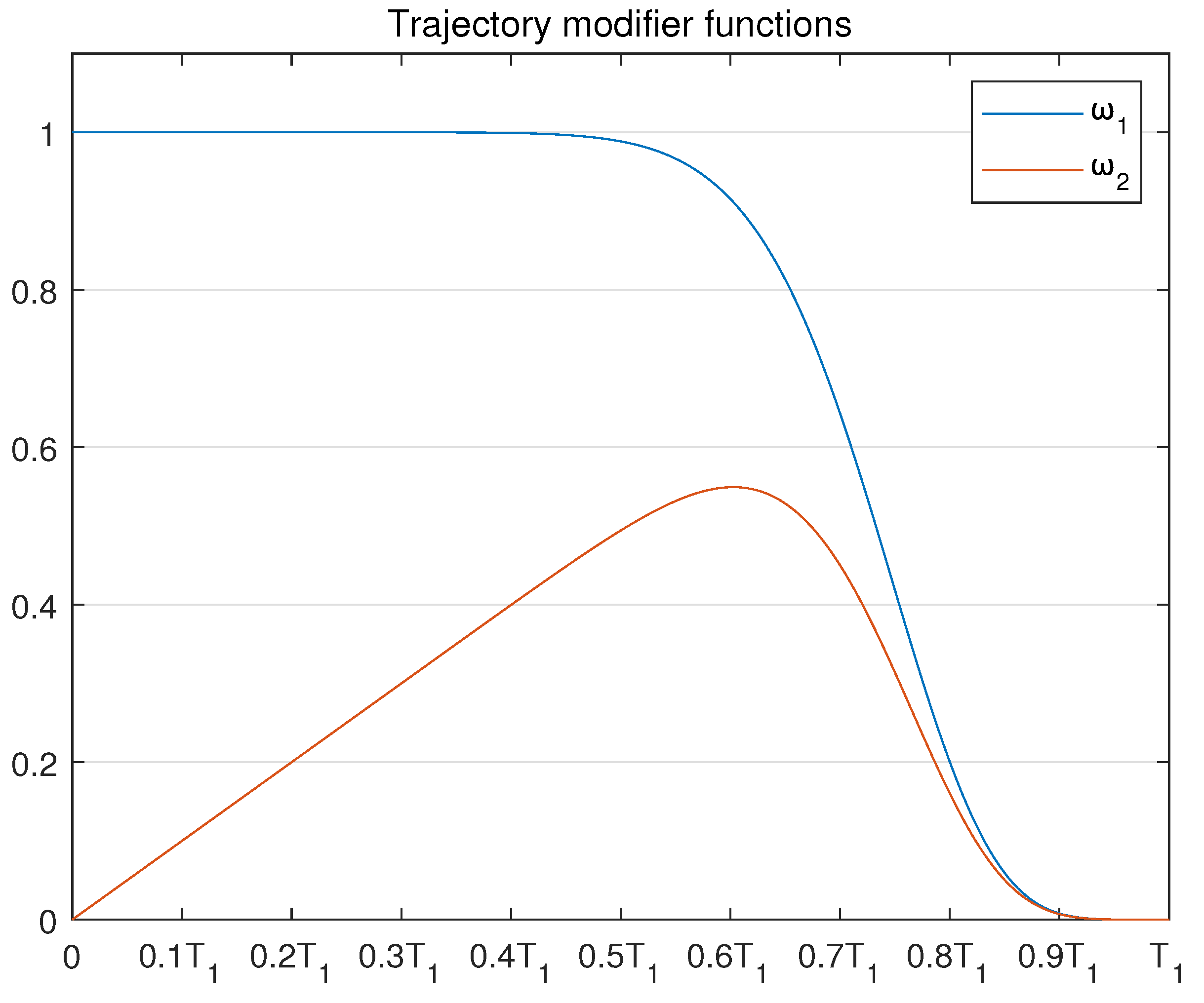
It can be seen from Figure 2 and (7) that the trajectory modifier function ${\omega }_1$ is 1 at $t=0$ and 0 at $t={\breve{T}}_1$, and ${\omega }_2$ is 0 at $t=0$ and 0 at $t={\breve{T}}_1$, all of which are continuously variable and differentiable. Combined with (5) and (6), we can see that no matter what $X_{1r,n}$ value is, $X_{1d,n}$ is 0 at $t=0$, which satisfies the condition that the initial condition of each iteration of the iterative learning controller is the same. And $X_{1d,n}$ is always equal to $X_{1r,n}$. The same is true for $X_{2d,n}$. Therefore, the new modifier trajectory method composed of (5)–(7) not only satisfies the conditions of ILC but also does not affect the tracking target of the system, which is useful.

Figure 2. The curves of trajectory modifier functions ${\omega }_1$ and ${\omega }_2$.

Remark 4.

Typically, conventional ILC controllers require the initial conditions to be identical for each iteration, meaning that the system’s initial tracking error is zero. However, this paper addresses the problem of non-repetitive trajectory tracking, which does not meet this requirement. The trajectory correction function helps to nullify the initial tracking error, allowing the system to align with the target estimation within a very short time frame. This is why the ILC-based controller in this paper can ensure system stability and maintain robust tracking performance. That is, with trajectory modifier function ${\omega }_j\left(t\right)$, one has $X_{jd,n}\left(0\right)=X_{j,n}\left(0\right)$ and $X_{jd,n}\left(t\right)=X_{jr,n}\left(t\right),j=1,2$ over $t\in [{\breve{T}}_1,\breve{T}]$. The proposed control strategy follows modified trajectories $X_{jd,n}\left(t\right)$. This implies that when dealing with non-repetitive trajectory tracking and random nonzero initial tracking errors, tracking performance may be slightly compromised during a short time interval $t\in [0,{\breve{T}}_1]$ at the beginning of each iteration. It is important to note that this trade-off is made to ensure that control objectives are achieved within $t\in [{\breve{T}}_1,\breve{T}]$. Since ${\breve{T}}_1$ can be configured to be as short as necessary, $[{\breve{T}}_1,\breve{T}]$ can closely approximate the entire $[0,\breve{T}]$ interval to a high degree of precision.

System state tracking errors are designed as follows:

$$\begin{array}{c}\hfill e_{j,n}\left(t\right)=X_{j,n}\left(t\right)-X_{jr,n}\left(t\right),j=1,2,n\in Z_{+}.\end{array}$$

(8)

Thus, system state constraints in every iteration are given by

$$\begin{array}{c}\hfill \left|\right|e_{1,n}\left(t\right)\left|\right|<k_{b,n}\left(t\right),t\in [{\breve{T}}_1,\breve{T}],\end{array}$$

(9)

where $\left|\right|·\left|\right|$ represents the Euclidean norm, and $k_{b,n}>0$ for $t\in [{\breve{T}}_1,\breve{T}]$ are the constraint functions of system position state tracking error at the nth iteration.

Remark 5.

In practice, ensuring the stable operation of a system with state constraints is a common and demanding control challenge. Many systems require position and velocity regulation to maintain stability. For instance, this is essential in SMT systems, which place circuit boards or lithographic presses for chip engraving [32]. Various other system states, such as acceleration and jerk, may also be constrained by system limitations or actuator torque boundaries.

For the sake of notation simplicity, time and state variables may be omitted in the subsequent analysis whenever this does not lead to any ambiguity.

4. Controller Design and BCEF

In this section, the control algorithm design is first presented. Fictitious state tracking errors are introduced such that

$$\begin{array}{cc}\hfill z_{1,n}& =X_{1,n}-X_{1d,n}\hfill \\ \hfill z_{2,n}& =X_{2,n}-{\sigma }_{1,n},\hfill \end{array}$$

(10)

where ${\sigma }_{1,n}$ is the stabilizing term as follows:

$$\begin{array}{cc}\hfill {\sigma }_{1,n}=& {\dot{X}}_{1d,n}+K_{\sigma ,n}{z}_{1,n}-K_1{z}_{1,n}co{s}^2\left(\frac{\pi z_{1,n}^T{z}_{1,n}}{2k_{b,n}^2}\right)\hfill \\ \hfill & -2K_{\sigma ,n}\frac{k_{b,n}^2}{\pi }\frac{z_{1,n}}{z_{1,n}^T{z}_{1,n}}sin\left(\frac{\pi z_{1,n}^T{z}_{1,n}}{2k_{b,n}^2}\right)\times cos\left(\frac{\pi z_{1,n}^T{z}_{1,n}}{2k_{b,n}^2}\right),\hfill \end{array}$$

(11)

where $K_1$ is a positive design constant and $K_{\sigma ,n}={\dot{k}}_{b,n}/k_{b,n}$.

The following controller is proposed by employing BCEF, inverse design, and the features of system (3),

$$\begin{array}{cc}\hfill u_n=& -{\breve{u}}_n{v}_{n}tanh\left(\frac{z_{2,n}^T{\breve{u}}_n{v}_n}{{ϵ}_n}\right),\hfill \end{array}$$

(12)

where ${ϵ}_n>0$ is designed from Lemma 2 at each iteration n, and $\breve{u}$ is the estimate of $\overline{u}=1/\underline{b}$ for the nth iteration in Remark 1, which is designed as

$$\begin{array}{cc}\hfill {\breve{u}}_n=& {\breve{u}}_{n-1}+K_{\breve{u}}{z}_{2,n}^T{v}_n,{\breve{u}}_0=0,\hfill \end{array}$$

(13)

where $K_{\breve{u}}>0$ is a designed parameter and $v_n$ is designed as

$$\begin{array}{cc}\hfill v_n=& {\breve{v}}_n+v_n^0\hfill \end{array}$$

(14)

$${\breve{v}}_n={\breve{v}}_{n-1}+K_v{z}_{2,n},{\breve{v}}_0=0$$

(15)

$$\begin{array}{cc}\hfill v_n^0=& -{\dot{\sigma }}_{1,n}+K_2{z}_{2,n}+\frac{z_{1,n}}{{cos}^2\left(\frac{\pi z_{1,n}^2}{2k_{b,n}^2}\right)}\hfill \\ \hfill & +{\breve{d}}_{n}tanh\left(\frac{z_{2,n}}{{ϵ}_n}\right)+{\breve{\theta }}_n{\breve{F}}_{n}tanh\left(\frac{z_{2,n}^T{\breve{F}}_n}{{ϵ}_n}\right),\hfill \end{array}$$

(16)

where $K_v>0$ is a design parameter, and $K_2>0$ is the designed control gain. ${\breve{d}}_n$ and ${\breve{\theta }}_n$ are the estimates for $\overline{d}$ and $\overline{\theta }$ at the nth iteration in Assumptions 2 and 3, respectively:

$$\begin{array}{cc}\hfill {\breve{d}}_n=& {\breve{d}}_{n-1}+K_d{z}_{2,n}^{T}tanh\left(\frac{z_{2,n}}{{ϵ}_n}\right),\hfill \end{array}$$

(17)

$$\begin{array}{cc}\hfill {\breve{\theta }}_n=& {\breve{\theta }}_{n-1}+K_{\theta }{z}_{2,n}^T{\breve{F}}_{n}tanh\left(\frac{z_{2,n}^T{\breve{F}}_n}{{ϵ}_n}\right),\hfill \end{array}$$

(18)

where $K_d>0$ and $K_{\theta }>0$ are design parameters.

The following BCEF is applied for facilitating further analysis,

$$\begin{array}{cc}\hfill E_n\left(t\right)=& V_{1,n}\left(t\right)+V_{2,n}\left(t\right)+V_{v,n}\left(t\right)+V_{\breve{u},n}\left(t\right)+V_{d,n}\left(t\right)+V_{\theta ,n}\left(t\right),\hfill \end{array}$$

(19)

$$\begin{array}{cc}\hfill V_{1,n}\left(t\right)=& \frac{k_{b,n}^2\left(t\right)}{\pi }tan\left(\frac{\pi z_{1,n}^T\left(t\right)z_{1,n}\left(t\right)}{2k_{b,n}^2\left(t\right)}\right)\hfill \end{array}$$

(20)

$$\begin{array}{cc}\hfill V_{2,n}\left(t\right)=& \frac{1}{2}{z}_{2,n}^T\left(t\right)z_{2,n}\left(t\right),\hfill \end{array}$$

(21)

$$\begin{array}{cc}\hfill V_{v,n}\left(t\right)=& \frac{1}{2K_v}{\int }_0^t{\breve{v}}_n^T\left(\tau \right){\breve{v}}_n\left(\tau \right)d\tau ,\hfill \end{array}$$

(22)

$$\begin{array}{cc}\hfill V_{\breve{u},n}\left(t\right)=& \frac{\underline{b}}{2K_{\breve{u}}}{\int }_0^t{\tilde{u}}_n^2\left(\tau \right)d\tau ,\hfill \end{array}$$

(23)

$$\begin{array}{cc}\hfill V_{d,n}\left(t\right)=& \frac{1}{2K_d}{\int }_0^t{\tilde{d}}_n^2\left(\tau \right)d\tau ,\hfill \end{array}$$

(24)

$$\begin{array}{cc}\hfill V_{\theta ,n}\left(t\right)=& \frac{1}{2K_{\theta }}{\int }_0^t{\tilde{\theta }}_n^2\left(\tau \right)d\tau ,\hfill \end{array}$$

(25)

where $\tilde{u}=\breve{u}-u$, $\tilde{d}=\breve{d}-d$ and $\tilde{\theta }=\breve{\theta }-\theta$.

Remark 6.

When designing the BECF, the following BLF from authors’ previous research [19] is chosen as the basis:

$$\begin{array}{c}\hfill V_n=\frac{k_{b,n}^2}{\pi }tan\left(\frac{\pi z_{1,n}^T{z}_{1,n}}{2k_{b,n}^2}\right),z_{1,n}\left(0\right)=0,\end{array}$$

(26)

where $z_{1,n}=X_{1,n}-X_{1d,n}$ is the fictitious position tracking error of the LMDGS. It follows from (26) that, if $|z_{1,n}|$ increases, $V_n$ tends to infinity, as $k_{b,n}$ is a predefined bound. Subsequently, a comprehensive analysis of the complete BCEF is carried out to prove the system’s state-tracking error convergence and ensure compliance with state constraints.

Remark 7.

The control algorithm in this paper is implemented using the designed BCEF and backstepping method. Based on Remark 6, $V_{1,n}$ is designed to constrain the system’s position state, $V_{2,n}$ ensures effective tracking of the system’s velocity, $V_{d,n}$ enables the system to adaptively handle external disturbances, $V_{\theta ,n}$ enhances robustness against parameter uncertainty and unmodeled dynamics, $V_{\breve{u},n}$ indicates the fault of the actuator, while $V_{v,n}$ and ensure stability of the iterative process. The ILC iteration form of the controller is in the form of P, and according to Lemma 1 and Lemma 2, the corresponding parts are derived through the designed BCEF and backstepping method. The controller is represented by (12) and (13), while (15) to (18) depict the iterative computation process. Although it may appear complex, it involves simple mathematical operations. For comparison with other algorithms, please refer to Section 6.2.

5. Convergence Analysis

This section provides evidence of convergence of system tracking errors and constraints on both system output and states.

Theorem 1.

(1) For LMDGS system (3) under actuator faults and Assumptions 1–3, given control law (12) with ILC laws (13)–(16), system state tracking errors $e_{1,n}\left(t\right)$ and $e_{2,n}\left(t\right)$ uniformly converge to 0 over $t\in [{\breve{T}}_1,\breve{T}]$, $n\to \infty$. That is, ${lim}_{n\to \infty }{e}_{j,n}=0$ over $t\in [{\breve{T}}_1,\breve{T}],j=1,2$.

(2) Constraints on system states are ensured within each iteration, that is $|{\mathit{e}}_{1,n}|<K_{1,n}$, and all system states are finite for $t\in [0,\breve{T}]$ during each iteration.

Proof of Theorem 1.

The proof consists of three steps. First, it is shown that $E_n\left(t\right)$ is finite. Next, uniform convergence of state tracking errors is demonstrated. Finally, it is proved that system states are finite. □

5.1. Finiteness of $E_n\left(t\right)$

First, it will be proved that the designed BCEF is bounded for $t\in [0,\breve{T}]$ over every iteration. For any iteration index n, and from the difference definition, one has

$$\begin{array}{cc}\hfill \Delta E_n\left(t\right)=& \Delta V_{1,n}+\Delta V_{2,n}+\Delta V_{v,n}+\Delta V_{\breve{u},n}+\Delta V_{d,n}+\Delta V_{\theta ,n}.\hfill \end{array}$$

(27)

Terms in (27) are checked in turn. For $\Delta V_{1,n}$, one has

$$\begin{array}{cc}\hfill \Delta V_{1,n}=& \frac{k_{b,n}^2\left(0\right)}{\pi }tan\left(\frac{\pi z_{1,n}^T\left(0\right)z_{1,n}\left(0\right)}{2k_{b,n}^2}\right)+{\int }_0^t\frac{z_{1,n}{\dot{z}}_{1,n}}{{cos}^2\left(\frac{\pi z_{1,n}^2\left(\tau \right)}{2k_{b,1}^2}\right)}d\tau -\frac{k_{b,n-1}^2}{\pi }tan\left(\frac{\pi z_{1,n-1}^T{z}_{1,n-1}}{2k_{b,n-1}^2}\right)\hfill \\ \hfill =& \frac{k_{b,n}^2\left(0\right)}{\pi }tan\left(\frac{\pi z_{1,n}^T\left(0\right)z_{1,n}\left(0\right)}{2k_{b,n}^2}\right)-\frac{k_{b,n-1}^2}{\pi }tan\left(\frac{\pi z_{1,n-1}^T{z}_{1,n-1}}{2k_{b,n-1}^2}\right)\hfill \\ \hfill & +{\int }_0^t(-(\frac{{\dot{k}}_{b,n}}{k_{b,n}})\frac{\pi z_{1,n}^T{z}_{1,n}}{{cos}^2(\frac{\pi z_{1,n}^T{z}_{1,n}}{2k_{b,n}^2})}+\frac{2k_{b,n}{\dot{k}}_{b,n}}{\pi }tan\left(\frac{\pi z_{1,n}^T{z}_{1,n}}{2k_{b,n}^2}\right)\hfill \\ \hfill & +\frac{z_{1,n}^T(z_{2,n}+{\sigma }_{1,n}-{\dot{X}}_{1d,n})}{{cos}^2(\frac{\pi z_{1,n}^T{z}_{1,n}}{2k_{b,n}^2})})d\tau .\hfill \end{array}$$

(28)

Designing stabilizing function ${\sigma }_{1,n}$ as in (11), and with conditions $z_{1,n}\left(0\right)=0$ for every iteration n under the designed trajectory modified function, one has

$$\begin{array}{cc}\hfill \Delta V_{1,n}<& {\int }_0^t\left(-K_1{z}_{1,n}^T{z}_{1,n}+\frac{z_{1,n}^T{z}_{2,n}}{{cos}^2\left(\frac{\pi z_{1,n}^2}{2k_{b,n}^2}\right)}\right)d\tau -\frac{k_{b,n-1}^2}{\pi }tan\left(\frac{\pi z_{1,n-1}^T{z}_{1,n-1}}{2k_{b,n-1}^2}\right).\hfill \end{array}$$

(29)

Similarly, $\Delta V_{2,n}$ leads to

$$\begin{array}{cc}\hfill \Delta V_{2,n}=& \frac{1}{2}{z}_{2,n}^T\left(0\right)z_{2,n}\left(0\right)+{\int }_0^t\left(z_{2,n}^T{\dot{z}}_{2,n}\right)d\tau -\frac{1}{2}{z}_{2,n-1}^T{z}_{2,n-1}.\hfill \end{array}$$

(30)

Note, that

$$\begin{array}{c}\hfill {\dot{X}}_{1d,n}\left(t\right)={\dot{X}}_{1r,n}\left(t\right)-\sum _{j=1}^2\dot{\omega }\left(t\right)(X_{jr,n}\left(0\right)-X_{j,n}\left(0\right)),\end{array}$$

(31)

where, at time $t=0$, ${\dot{\omega }}_2\left(0\right)=1$, and ${\dot{\omega }}_1\left(0\right)=0$, one has ${\dot{X}}_{1d,n}\left(0\right)=X_{2r,n}\left(0\right)-(X_{2r,n}\left(0\right)-X_{2,n}\left(0\right))=X_{2,n}\left(0\right)$. Thus, $z_{2,n}\left(0\right)=X_{2,n}\left(0\right)-{\sigma }_{1,n}\left(0\right)=0$.

At the final step of the backstepping process, the control signal comes into effect. Examining the dynamics of ${\dot{z}}_{2,n}$, it yields

$$\begin{array}{c}\hfill {\dot{z}}_{2,n}=-{\dot{\sigma }}_{1,n}+{\mathrm{\Theta }}_n^T{F}_n+d_n+G_n{\rho }_n{u}_n+G_n{\varphi }_n.\end{array}$$

(32)

Furthermore,

$$\begin{array}{c}\hfill \Delta V_{2,n}=\frac{1}{2}{z}_{2,n}^T\left(0\right)z_{2,n}\left(0\right)+{\int }_0^t\left(z_{2,n}^T{\dot{z}}_{2,n}\right)d\tau -\frac{1}{2}{z}_{2,n-1}^T{z}_{2,n-1},\end{array}$$

(33)

where $z_{2,n}\left(0\right)=0$ follows from the design of the modified reference and modifier functions. For term $z_{2,n}^T{\dot{z}}_{2,n}$ one has

$$\begin{array}{cc}\hfill z_{2,n}^T{\dot{z}}_{2,n}=& -z_{2,n}^T{\dot{\sigma }}_{1,n}+z_{2,n}^T{\mathrm{\Theta }}_n^T{F}_n+z_{2,n}^T(d_n+G_n{\varphi }_n)+z_{2,n}^T{G}_n{\rho }_n{u}_n.\hfill \end{array}$$

(34)

Note, that

$$\begin{array}{cc}\hfill z_{2,n}^T{\mathrm{\Theta }}_n^T{F}_n& \le \left|\right|z_{2,n}\left|\right|\tilde{\theta }\left|\right|F_n\left|\right|<\overline{\theta }{K}_l{ϵ}_n+\overline{\theta }{z}_{2,n}^T{F}_{n}tanh\left(\frac{z_{2,n}^T{F}_n}{{ϵ}_n}\right),\hfill \end{array}$$

(35)

and

$$\begin{array}{cc}\hfill z_{2,n}^T(d_n+G_n{\varphi }_n)& \le \left|\right|z_{2,n}\left|\right|\tilde{d}<\overline{d}{K}_l{ϵ}_n+\overline{d}{z}_{2,n}^{T}tanh\left(\frac{z_{2,n}}{{ϵ}_n}\right).\hfill \end{array}$$

(36)

Concerning the control input, given Assumption 1 and Lemma 1, $\mu =1/\underline{b}$, one obtains

$$\begin{array}{cc}\hfill z_{2,n}^T{G}_n{\rho }_n{u}_n& <{ϵ}_n\underline{b}-\underline{b}{\breve{u}}_n{z}_{2,n}^T{v}_k+\underline{b}\mu z_{2,n}^T{v}_k-\underline{b}\mu z_{2,n}^T{v}_k<{ϵ}_n\underline{b}-z_{2,n}^T{v}_n-\underline{b}{\tilde{u}}_n{z}_{2,n}^T{v}_k.\hfill \end{array}$$

(37)

Considering (14)–(16), (33) is transformed into

$$\begin{array}{cc}\hfill \Delta V_{2,n}<& {\int }_0^t(-z_{2,n}^T{\breve{v}}_n-z_{2,n}^T{v}_n\underline{b}{\tilde{u}}_n+{ϵ}_n(\underline{b}+\overline{d}{K}_l+\overline{\theta }{K}_l)-\frac{z_{1,n}^T{z}_{2,n}}{{cos}^2\left(\frac{\pi z_{1,n}^2}{2k_{b,n}^2}\right)}-K_2{z}_{2,n}^T{z}_{2,n}\hfill \\ \hfill & -{\tilde{d}}_n{z}_{2,n}^{T}tanh\left(\frac{z_{2,n}}{{ϵ}_n}\right)-{\tilde{\theta }}_n{z}_{2,n}^T{F}_{n}tanh\left(\frac{z_{2,n}^T{F}_n}{{ϵ}_n}\right))d\tau -\frac{1}{2}{z}_{2,n-1}^T{z}_{2,n-1}.\hfill \end{array}$$

(38)

Regarding terms $\Delta V_{v,n}$, $\Delta V_{\breve{u},n}$, $\Delta V_{d,n}$, and $\Delta V_{\theta ,n}$, starting with $\Delta V_{v,n}$ it can be obtained that

$$\begin{array}{cc}\hfill \Delta V_{v,n}\left(t\right)=& \frac{1}{2K_v}{\int }_0^t{({\breve{v}}_n+{\breve{v}}_{n-1})}^T({\breve{v}}_n-{\breve{v}}_{n-1})d\tau \hfill \\ \hfill =& \frac{1}{2K_v}{\int }_0^t{(2{\breve{v}}_n-K_v{z}_{2,n})}^T\left(K_v{z}_{2,n}\right)d\tau \le {\int }_0^t{z}_{2,n}^T{\breve{v}}_{n}d\tau .\hfill \end{array}$$

(39)

Similarly,

$$\begin{array}{cc}\hfill \Delta V_{\breve{u},n}\left(t\right)=& \frac{\underline{b}}{2K_{\breve{u}}}{\int }_0^t{\tilde{u}}_n^2-{\tilde{u}}_{n-1}^{2}d\tau \le {\int }_0^t\underline{b}{z}_{2,n}^T{v}_n{\tilde{u}}_{n}d\tau .\hfill \end{array}$$

(40)

$$\begin{array}{cc}\hfill \Delta V_{d,n}\left(t\right)=& \frac{1}{2K_d}{\int }_0^t{\tilde{d}}_n^2-{\tilde{d}}_{n-1}^{2}d\tau \le {\int }_0^t{\tilde{d}}_n{z}_{2,n}^{T}tanh\left(\frac{z_{2,n}}{{ϵ}_n}\right)d\tau .\hfill \end{array}$$

(41)

$$\begin{array}{cc}\hfill \Delta V_{\theta ,n}\left(t\right)=& \frac{1}{2K_{\theta }}{\int }_0^t{\tilde{\theta }}_n^2-{\tilde{\theta }}_{n-1}^{2}d\tau \le -{\tilde{\theta }}_n{z}_{2,n}^T{F}_{k}tanh\left(\frac{z_{2,n}^T{F}_k}{{ϵ}_n}\right)d\tau .\hfill \end{array}$$

(42)

Therefore, from (29), (38)–(42),

$$\begin{array}{cc}\hfill \Delta E_n=& {\int }_0^t\left(-\sum _{j=1}^2{K}_j{z}_{j,n}^T{z}_{j,n}\right)d\tau +{ϵ}_n(\underline{b}+\overline{d}{K}_l+\overline{\theta }{K}_l)\breve{T}\hfill \\ \hfill & -\frac{k_{b,n-1}^2}{\pi }tan\left(\frac{\pi z_{1,n-1}^T{z}_{1,n-1}}{2k_{b,n-1}^2}\right)-\frac{1}{2}{z}_{2,n-1}^T{z}_{2,n-1}.\hfill \end{array}$$

(43)

To prove $E_n$ is finite, from (43), one has

$$\begin{array}{cc}\hfill E_n\left(t\right)\le & E_1\left(t\right)-\sum _{k=2}^n{\int }_0^t\left(-\sum _{j=1}^2{K}_j{z}_{j,k}^T{z}_{j,k}\right)d\tau +\sum _{k=2}^n{ϵ}_k(\underline{b}+\overline{d}{K}_l+\overline{\theta }{K}_l)\breve{T}\hfill \\ \hfill & -\sum _{k=2}^n\frac{k_{b,k-1}^2}{\pi }tan\left(\frac{\pi z_{1,k-1}^T{z}_{1,k-1}}{2k_{b,k-1}^2}\right)-\sum _{k=2}^n\frac{1}{2}{z}_{2,k-1}^T{z}_{2,k-1}.\hfill \end{array}$$

(44)

From Lemma 2, ${\sum }_{k=2}^n{ϵ}_k(\underline{b}+\overline{d}{K}_l+\overline{\theta }{K}_l)\breve{T}$ is bounded. When $n=1$, $E_1\left(t\right)$ is bounded. Similarly for $\Delta E_n\left(t\right)$,

$$\begin{array}{cc}\hfill {\dot{E}}_1=& {\dot{V}}_{1,1}+{\dot{V}}_{2,1}+{\dot{V}}_{v,1}+{\dot{V}}_{\breve{u},1}+{\dot{V}}_{d,1}+{\dot{V}}_{\theta ,1}\hfill \\ \hfill \le & -z_{2,1}^T{\breve{v}}_1-z_{2,1}^T{v}_1\underline{b}{\tilde{u}}_1+{ϵ}_1(\underline{b}+\overline{d}{K}_l+\overline{\theta }{K}_l)-\sum _{j=1}^2{K}_j{z}_{j,1}^T{z}_{j,1}-{\tilde{d}}_1{z}_{2,1}^{T}tanh\left(\frac{z_{2,1}}{{ϵ}_1}\right)\hfill \\ \hfill & -{\tilde{\theta }}_1{z}_{2,1}^T{F}_{n}tanh\left(\frac{z_{2,1}^T{F}_k}{{ϵ}_1}\right)+\frac{1}{2K_v}{\breve{v}}_1^T{\breve{v}}_1+\frac{\underline{b}}{2K_{\breve{v}}}{\tilde{u}}_1^2+\frac{1}{2K_d}{\tilde{d}}_1^2+\frac{1}{2K_{\theta }}{\tilde{\theta }}_1^2.\hfill \end{array}$$

(45)

From (13), (15), (17) and (18), one can obtain

$$\begin{array}{cc}\hfill {\breve{u}}_1=& K_{\breve{u}}{z}_{2,1}^T{v}_1,{\breve{v}}_1=K_{\breve{v}}{z}_{2,1},{\breve{d}}_1=K_d{z}_{2,1}^{T}tanh\left(\frac{z_{2,1}}{{ϵ}_1}\right),\hfill \\ \hfill {\breve{\theta }}_1=& K_{\theta }{z}_{2,1}^T{F}_{1}tanh\left(\frac{z_{2,1}^T{F}_1}{{ϵ}_1}\right).\hfill \end{array}$$

(46)

By introducing (46) into (45) and simplifying it,

$$\begin{array}{cc}\hfill {\dot{E}}_1<& {ϵ}_1(\underline{b}+\overline{d}{K}_l+\overline{\theta }{K}_l)+\frac{\underline{b}{\tilde{u}}_1^2}{2K_{\breve{u}}}+\frac{{\tilde{d}}_1^2}{2K_d}+\frac{{\tilde{\theta }}_1^2}{2K_{\theta }}<\infty .\hfill \end{array}$$

(47)

Hence, $E_1\left(t\right)$ is finite over $t\in [0,\breve{T}]$. When $n=2$, from (44) and Lemma 2, $E_1\left(t\right)$, ${ϵ}_2(\underline{b}+\overline{d}{K}_l+\overline{\theta }{K}_l)$ and $\frac{k_{b,1}^2}{\pi }tan\left(\frac{\pi z_{1,1}^T{z}_{1,1}}{2k_{b,1}^2}\right)$ are finite and nonnegative. Thus, $E_2\left(t\right)$ is also finite over $t\in [0,\breve{T}]$. Similarly, it can be concluded that for any iteration n, $E_n\left(t\right)$ is finite over $t\in [0,\breve{T}]$.

5.2. Convergence of State Tracking Errors

5.2.1. Fictitious State Tracking Errors

Based on the previous analysis, when $n\to \infty$, it follows that

$$\begin{array}{cc}\hfill \underset{n\to \infty }{lim}{E}_n\left(t\right)\le & E_1\left(t\right)-\underset{n\to \infty }{lim}\sum _{k=2}^n{\int }_0^t\left(\sum _{j=1}^2{K}_j{z}_{j,k}^T{z}_{j,k}\right)d\tau +\underset{n\to \infty }{lim}\sum _{k=2}^n{ϵ}_k(\underline{b}+\overline{d}{K}_l+\overline{\theta }{K}_l)\breve{T}\hfill \\ \hfill & -\underset{n\to \infty }{lim}\sum _{k=2}^n\frac{k_{b,k-1}^2}{\pi }tan\left(\frac{\pi z_{1,k-1}^T{z}_{1,k-1}}{2k_{b,k-1}^2}\right)-\underset{n\to \infty }{lim}\sum _{k=2}^n\frac{1}{2}{z}_{2,k-1}^T{z}_{2,k-1}.\hfill \end{array}$$

(48)

Since $E_n\left(t\right)$ is positive and both $C_1=E_1\left(t\right)$ and $C_2={lim}_{n\to \infty }{\sum }_{k=2}^n{ϵ}_k(\underline{b}+\overline{d}{K}_l+\overline{\theta }{K}_l)\breve{T}$ are bounded. $[\left(k_{b,k-1}^2\right)/\pi ]tan[\left(\pi z_{1,k-1}^T\right)/2k_{b,k-1}^2]$≥$(1/2)z_{1,k-1}^T{z}_{1,k-1}$, hence,

$$\begin{array}{cc}\hfill \underset{n\to \infty }{lim}{E}_n\left(t\right)\le & C_1+C_2-\underset{n\to \infty }{lim}\sum _{k=2}^n\sum _{j=1}^2\frac{1}{2}{z}_{j,k}^T{z}_{j,k}-\underset{n\to \infty }{lim}\sum _{k=2}^n{\int }_0^t\left(\sum _{j=1}^2{K}_j{z}_{j,k}^T{z}_{j,k}\right)d\tau >0.\hfill \end{array}$$

(49)

Since $K_j\ge 0$, then ${lim}_{n\to \infty }{\sum }_{j=1}^2{z}_{j,n}^T{z}_{j,n}=0$. Thus,

$$\begin{array}{c}\hfill \underset{n\to \infty }{lim}{z}_{j,n}\left(t\right)=0,j=1,2,t\in [0,\breve{T}],\end{array}$$

(50)

and uniform convergence of the system fictitious full state tracking error is demonstrated.

5.2.2. State Tracking Errors

State tracking errors converge uniformly in $[0,\breve{T}]$. For position state tracking error $e_{1,n}$, from (5), (7), (8), (10) and (50), it follows that ${lim}_{n\to \infty }{e}_{1,n}\left(t\right)\to 0$ for $t\in [{\breve{T}}_1,\breve{T}]$. Similarly, from (6)–(8), (10) and (50), as $n\to 0$, ${\sigma }_{1,n}\to {\dot{X}}_{1d,n}=X_{2,n}$, and $z_{2,n}=X_{2,n}-{\sigma }_{1,n}=e_{2,n}$ over $t\in [{\breve{T}}_1,\breve{T}]$. Since $z_{2,n}$ converges uniformly, $e_{2,n}$ also converges uniformly to 0 as $n\to \infty$ for $t\in [{\breve{T}}_1,\breve{T}]$. In other words,

$$\begin{array}{c}\hfill \underset{n\to \infty }{lim}{e}_{j,n}\left(t\right)=0,t\in [{\breve{T}}_1,\breve{T}],j=1,2.\end{array}$$

(51)

5.3. Boundedness of System States

Since $E_n\left(t\right)$ has been proven to be finite, BCEF $[2k_{b,n}^2/\pi ]tan(\pi z_{1,n}^T{z}_{1,n}/2k_{b,n}^2)\le E_n<\infty$ is bounded. Hence, by scaling transformation, one can obtain

$$\begin{array}{c}\hfill \left|\right|z_{1,n}\left|\right|\le \sqrt{\frac{2k_{b,n}^2}{\pi }{tan}^{-1}(\frac{E_n\pi }{k_{b,n}^2})}<\sqrt{\frac{2k_{b,n}^2}{\pi }\frac{\pi }{2}}=k_{b,n}.\end{array}$$

(52)

Therefore, position tracking error $z_{1,n}$ is always smaller than bound $k_{b,n}$. Thus $X_{1,n}$ is bounded during every iteration over $[{\breve{T}}_1,\breve{T}]$. From (50), during $[0,{\breve{T}}_1]$$\left|\right|z_{1,n}\left|\right|=\left|\right|X_{1,n}-X_{1r,n}-{\sum }_{j=1}^2{\omega }_j(X_{jr,n}-X_{j,n})\left|\right|$. Besides, $X_{1r,n}$, $\left|\right|(X_{jr,n}-X_{j,n})\left|\right|$ and ${\omega }_j$ are bounded at $j=1,2$, hence $X_{1,n}$ is bounded during $t\in [0,\breve{T}]$ on each iteration.

Similarly, it can be concluded that $X_{2,n}$ is finite during $t\in [0,\breve{T}]$ on every iteration. Since both $z_{2,n}$ and ${\sigma }_{1,n}$ are finite from (11) and $z_{2,n}=X_{2,n}-{\sigma }_{1,n}$, $X_{1,n}$ is also bounded.

Remark 8.

$n\to \infty$, $z_{1,n}$ and $z_{2,n}$ converges to zero uniformly, and ${\mathit{e}}_{1,n}$ and ${\mathit{e}}_{2,n}$ tend to 0 as well. Hence, as iterations progress, the system’s state tracking error achieves uniform convergence, while also ensuring the boundedness of both system output and states.

Remark 9.

Theoretically, ${\breve{T}}_1$ can be chosen arbitrarily small to allow $[{\breve{T}}_1,\breve{T}]$ to approximate the entire iteration period $[0,\breve{T}]$ with high precision. However, since ${\breve{T}}_1$ appears in the denominator of the desired trajectory correction function, making ${\breve{T}}_1$ excessively small can result in excessively large control signals, which is detrimental. Therefore, the value of ${\breve{T}}_1$ should be balanced according to the specific requirements of practical applications.

Remark 10.

The analysis in this chapter provides comprehensive evidence for the theoretical effectiveness of the control algorithm proposed in this paper. This approach combines iterative learning with backstepping cooperative design, achieving system stability without requiring prior knowledge of dynamic models or parameters. By using the barrier composite energy function, this controller effectively regulates system stability even when operating under state constraints. The instability issues caused by actuator failures are properly addressed, thus enhancing the robustness of the controller. The design of the trajectory correction function further extends its applicability.

6. Experimental Results and Discussion

In this section, experimental results are presented and discussed, demonstrating the efficacy and practicality of the proposed methodology.

6.1. Experimental Platform

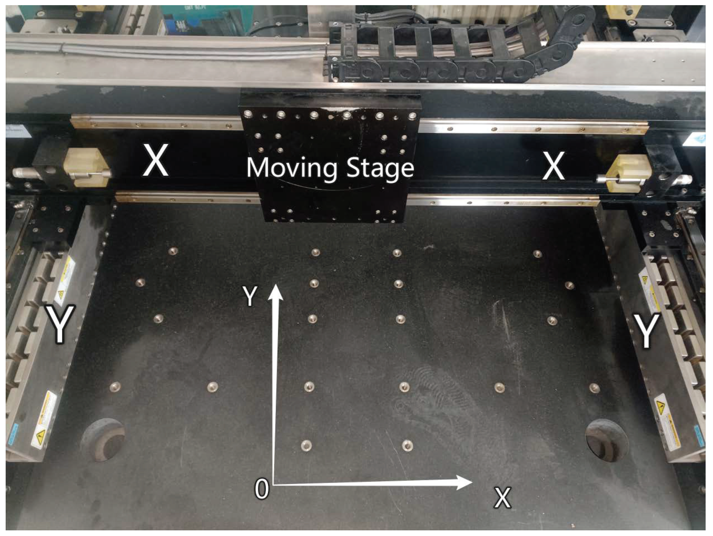
Experiments have been conducted on the LMDGS (Akribis System, Shanghai, China) depicted in Figure 3. Both the X and Y axes are driven by flat linear motors. Given the extended span of the X-axis, identical motor drives are used on either side of the Y-axis. It is important to note that this article does not delve into the synchronization issue of the Y-axis. Hence, in the experiments, the Y-axis is considered as a single-drive axis. To provide accurate feedback for the entire system, optical encoders with 50 nm resolution are strategically positioned alongside the rail. The control algorithm runs on an industrial computer connected to an EtherCAT network, enabling closed-loop control of the entire experimental platform. The master controller operates with a control period of h = 1 ms. The remaining parameters of the experimental platform are detailed in Table 1.

Figure 3. Experimental platform.

Table 1. Experimental platform parameters.

Index	m	${\mathit{k}}_{\mathit{v}}$	${\mathit{k}}_{\mathit{c}}$	${\mathit{k}}_{\mathit{m}}$	${\mathit{k}}_{\mathit{f}}$	f
Unit	kg	N·s/mm	N	1	N/V	1
X	15	0.1	3	0.03	10	9.738
Y	25	0.1	3	0.03	80	30.531

6.2. Validation Experiments

The practical effectiveness and merits of the proposed controller are demonstrated in two experimental scenarios. A varying curvilinear ellipse where the X and Y frequencies are identical is used as the target trajectory to show the versatility of the approach. The first experiment validates the usefulness of the developed ILC scheme for tracking the elliptical target trajectory. By introducing variations in state and input constraints, the study proves the ability of the system to properly work in state- and input-constrained scenarios. The second experiment involves the application of three different methods for tracking the elliptical target trajectory, followed by a comparative analysis of the tracking and control performance among these approaches.

The target trajectory is an ellipse that varies with iteration index n, described as follows (units are meters)

$$\begin{array}{c}\hfill \left\{\begin{array}{cc}x\left(t\right)\hfill & =0.05\ast (sin\left(\frac{\pi }{2}t\right)+sin\left(n\right)),\hfill \\ y\left(t\right)\hfill & =0.02\ast (1-cos\left(\frac{\pi }{2}t\right)+sin\left(n\right)),\hfill \\ t\hfill & ⩾0.\hfill \end{array}\right.\end{array}$$

(53)

For comparison purposes, two additional commonly used control methods, namely PID and adaptive robust control (ARC), are also implemented for tracking the same trajectory. Notably, the learning law of the proposed ILC is also based on the PD form. For a fair comparison, the same trajectory modifier function is used in all three methods, subsequently referred to as TMPID, TMARC, and TMILC. (“Position” is abbreviated as “Pos.” and “Velocity” as “Vel.”.)

6.2.1. TMILC Performance Experiment

To validate the effectiveness of the proposed TMILC in mitigating the impact of actuator faults, in this experiment actuator power faults for the X and Y axes are all introduced as $p_n=0.8+0.2e^{-5(t-(n-1)\breve{T})}$ and ${\varphi }_n=-0.0005(n-1)$. The modifier function parameters are set as $\breve{T}=4,{\breve{T}}_1=1$. Detailed control parameters can be found in the next subsubsection.

Remark 11.

The form of actuator faults simulated in this experiment largely encompasses common scenarios in engineering applications [33]. The multiplicative component of the actuator fault represents the loss of actuator power, indicating a gradual decrease. The additive component accounts for changes in friction and other resistance. During the experiment, the fault becomes active from the second iteration ($n=2$) at $t=4$ s, and it continues to change with each subsequent iteration.

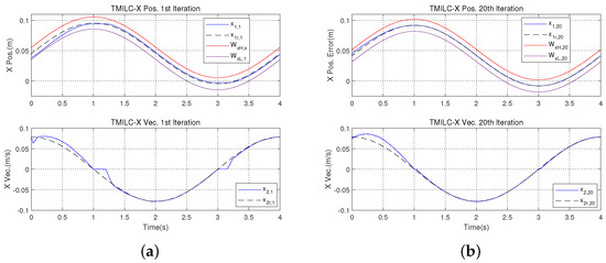
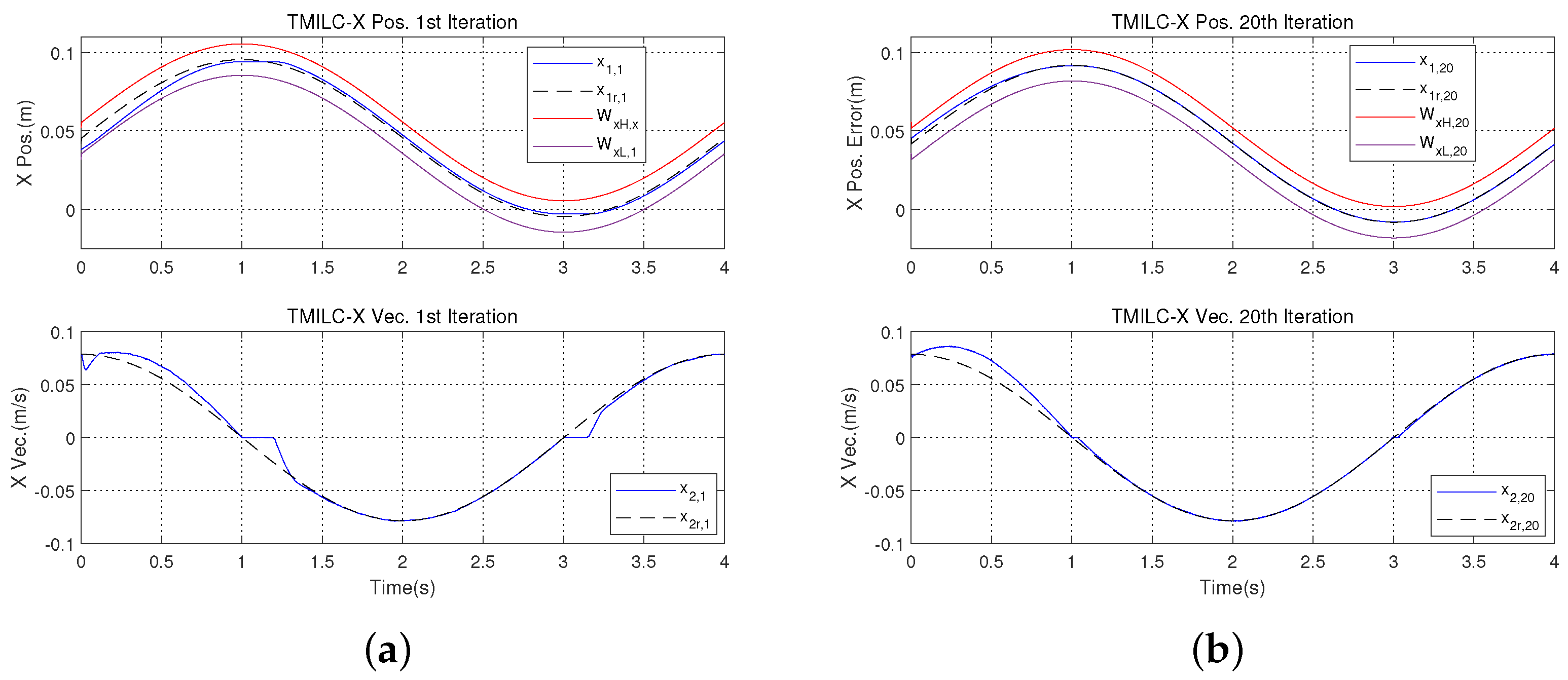
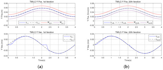
Figure 4 depicts the changes in position and velocity states of the X-axis during the first and twentieth iterations, respectively. It is clear that the position and velocity states of the X-axis are closer to the corresponding target trajectory as iteration progresses, nearly overlapping it. Additionally, throughout all the iterations, the position state of the X-axis is consistently well-constrained within the predetermined limits. It is worth noting that these effects persist even during the trajectory-modified period (t = [0, 1]). Similar conclusions can be drawn from the state curve plots of the Y-axis in Figure 5. Therefore, under the predefined position states and actuator faults, the proposed TMILC method effectively tracks the non-repetitive target trajectory, validating the contributions and usefulness of this work.

Figure 4. Evolution of X−states $x_{1,n}$, $x_{1r,n}$, $x_{2,n}$ and $x_{2r,n}$ under constraints $W_{xH,n}$ and $W_{xL,n}$. (a) During the first iteration, $n=1$. (b) During the twentieth iteration, $n=20$.

Figure 5. Evolution of Y−states $y_{1,n}$, $y_{1r,n}$, $y_{2,n}$ and $y_{2r,n}$ under constraints $W_{yH,n}$ and $W_{yL,n}$. (a) During the first iteration, $n=1$. (b) During the twentieth iteration, $n=20$.

6.2.2. Comparison of TMARC, TMPID, and TMILC

For the sake of fair comparison, in the experiments, the same reference trajectory is used in all methods, and the parameters of each method are carefully selected as follows to obtain the configuration with the best performance.

TMILC: Control parameters are selected as $K_1=[6,8]$ and $K_2=[2,3]$. TMILC gains are chosen as $K_{\breve{u}}=[0.2,0.1],K_v=[0.2,0.1],K_d=[0.2,0.1]$ and $K_{\theta }=[0.2,0.1]$. System constraints are $k_{b,n}=[0.01,0.01]$.

TMARC: The Coulomb friction nonlinear term is $S_f^{\ast }\left(x_2\right)=$ arctan(800$x_2$), where arctan(800$x_2$) is a continuous smooth function and $x_2$ is the system velocity. $V_s=$$-K_{s}p$$-K_{e}e$$-K_a{\parallel e\parallel }^{2}p$. Gains are set to $K_s=$ diag[9.3, 3.2], $K_e=$ diag[320, 310], and $K_a=$ diag[500, 500]. The initial parameter vector is chosen as $\theta =$ [0.05, 0.1, 0.3, 0.08, 0.03, 0.02, 0, 0]. The range of $\theta$ is selected as ${\theta }_{min}=$ [0.03, 0.7, 0.2, 0.06, 0.01, 0.01, −0.02, −0.04] and ${\theta }_{max}=$ [0.07, 0.13, 0.4, 0.1, 0.05, 0.03, 0.02, 0.04].

TMPID: Gains are $P=$ 960, $I=$ 75, and $D=$ 9850.

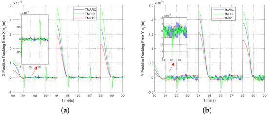
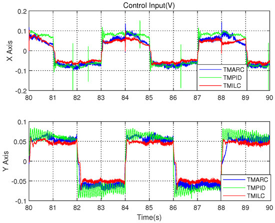
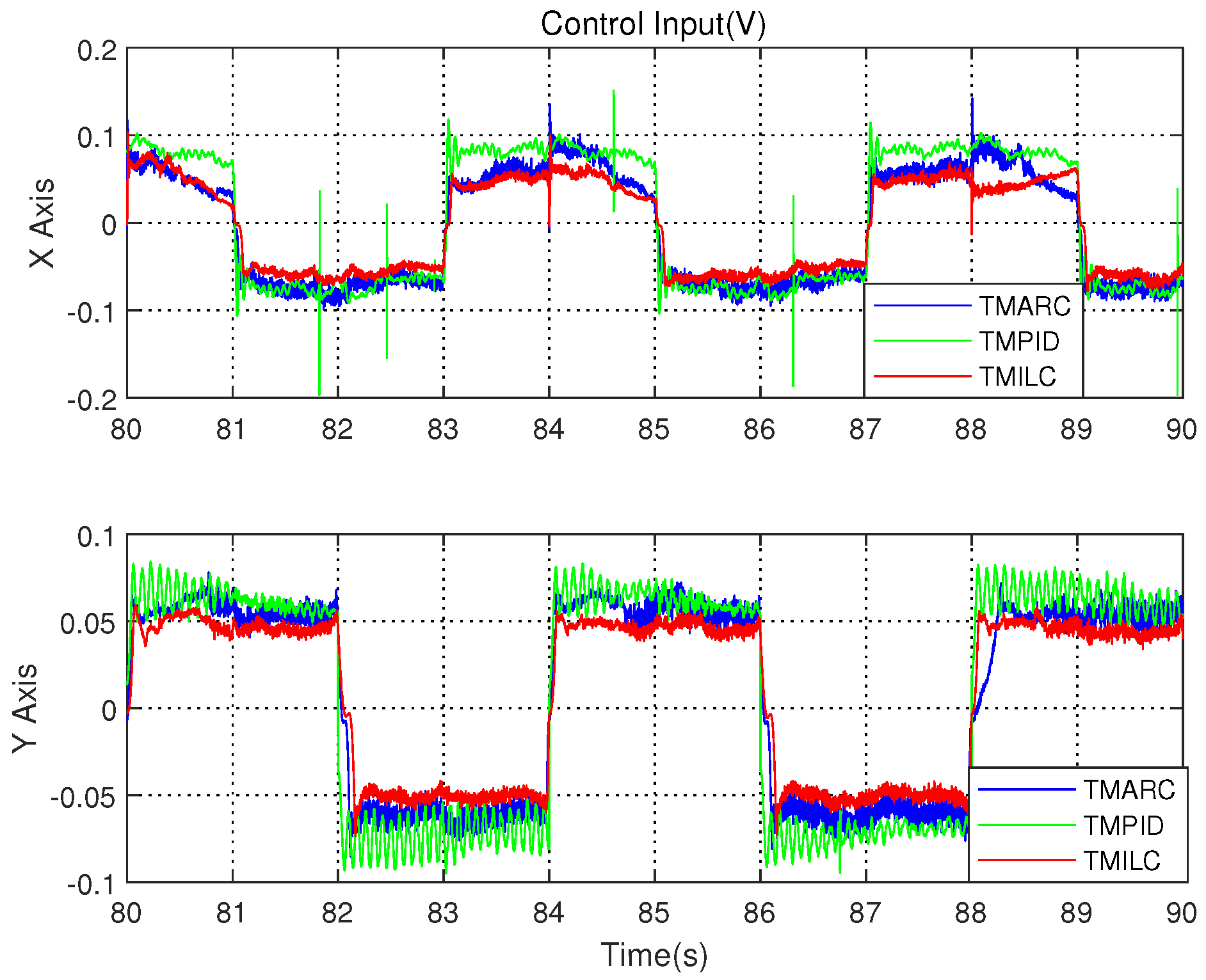
After carrying out numerous experiments, $t=[80,90]$ turned out to be the time interval where results for all three methods stabilized with minimal errors. From Figure 6a, it is evident that the X-axis tracking error of TMILC is smaller compared to that of TMARC and TMPID. Moreover, the X-axis tracking error curve of TMILC exhibits better smoothness with minimal fluctuations, whereas for TMARC and TMPID noticeable peaks appear. At $t=4n$, when the correction function is activated, TMILC exhibits smaller and faster-reducing peaks. The Figure 6b shows the same behavior for the Y-axis tracking error. Figure 7 depicts output curves for the X and Y axes of all three methods during the time interval $t=[80,90]$. It is clear that TMILC’s output curves have smaller amplitudes, smoother trajectories, and lower fluctuations, resulting in lower power demand on the actuator.

Figure 6. The position tracking error for TMARC, TMPID, and TMILC. (a) X-axis. (b) Y-axis.

Figure 7. Control inputs of X and Y axes for TMARC, TMPID, and TMILC.

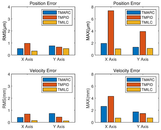
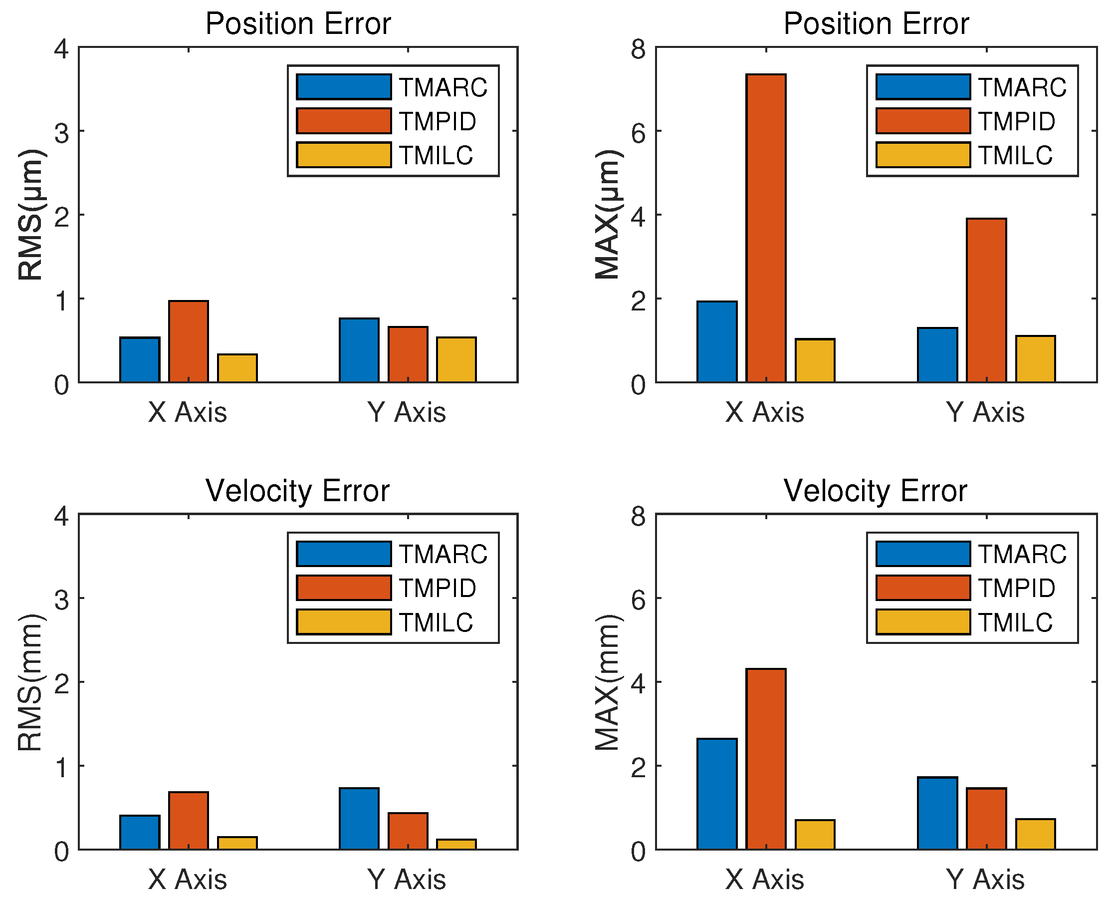
To further demonstrate the superiority of the proposed method, a quantitative analysis of position and velocity tracking errors has been performed. The results are listed in Table 2 and Table 3, where

$$\begin{array}{c}\hfill RMSError={\left(\frac{1}{n}\sum _{j=1}^n{e}^2\left(j\right)\right)}^{\frac{1}{2}}.\end{array}$$

(54)

Table 2. Position tracking error $e_1$ for TMILC, TMARC, and TMPID.

Index	TMILC	TMARC	TMPID
Max$|e_1|X$	1.0315$\times {10}^{-5}$	1.9304$\times {10}^{-5}$	7.3413$\times {10}^{-5}$
Max$|e_1|Y$	1.1047$\times {10}^{-5}$	1.2986$\times {10}^{-5}$	3.9029$\times {10}^{-5}$
RMS $e_{1}X$	3.3453$\times {10}^{-6}$	5.3372$\times {10}^{-6}$	9.7100$\times {10}^{-6}$
RMS $e_{1}Y$	5.3772$\times {10}^{-6}$	7.6146$\times {10}^{-6}$	6.6105$\times {10}^{-6}$

Table 3. Velocity tracking error $e_2$ for TMILC, TMARC, and TMPID.

Index	TMILC	TMARC	TMPID
Max$|e_2|X$	6.9881$\times {10}^{-4}$	2.6380$\times {10}^{-3}$	4.3013$\times {10}^{-3}$
Max$|e_2|Y$	7.2846$\times {10}^{-4}$	1.7175$\times {10}^{-3}$	1.4549$\times {10}^{-3}$
RMS $e_{2}X$	1.4865$\times {10}^{-4}$	4.0457$\times {10}^{-4}$	6.8210$\times {10}^{-4}$
RMS $e_{2}Y$	1.1971$\times {10}^{-4}$	7.3033$\times {10}^{-4}$	4.3452$\times {10}^{-4}$

From Figure 8 and the data in Table 2, it is evident that TMILC exhibits superior performance in position tracking error for both the X and Y axes. The absolute maximum value of its X-axis position tracking error is approximately half of that of TMARC and TMPID. Its RMS error is about one-third of that of TMARC and approximately equal to that of TMPID. Similar conclusions apply to the Y-axis position tracking error, as both the absolute maximum and RMS values of TMILC are smaller than those of TMARC and TMPID. From Table 3 and Figure 8, it is also clear that, in terms of velocity tracking, TMILC also outperforms TMARC and TMPID.

Figure 8. Max and RMS of state tracking errors e₁, e₂ for TMARC, TMPID and TMILC.

7. Conclusions

This article introduces a novel adaptive iterative learning fault-tolerant controller to address state constraints and actuator failures in LMDGSs without requiring a priori knowledge of the system’s precise model. With this adaptive iterative learning fault-tolerant controller, LMDGSs states comply with predefined constraint conditions. Furthermore, it effectively handles both multiplicative and additive actuator faults in LMDGSs. These conclusions also apply to scenarios involving non-repetitive target trajectories, thanks to the introduction of a trajectory modifier function. The advantages of the proposed method outlined above have been validated in practical experiments on LMDGSs. Furthermore, it exhibited excellent performance, surpassing that of comparative methods, even in scenarios involving actuator faults and system constraints. Future research will focus on developing a chatting-free adaptive control algorithm for LMDGSs to achieve perfect trajectory tracking performance.

References

- Zhou, S.; Shi, Y.; Wang, D.; Xu, X.; Xu, M.; Deng, Y. Election Optimizer Algorithm: A New Meta-Heuristic Optimization Algorithm for Solving Industrial Engineering Design Problems. Mathematics 2024, 12, 1513. [Google Scholar] [CrossRef] [Scilit]
- Pan, H.; Chang, X.; Sun, W. Multitask Knowledge Distillation Guides End-to-End Lane Detection. IEEE Trans. Ind. Inform. 2023, 19, 9703–9712. [Google Scholar] [CrossRef] [Scilit]
- Pan, H.; Hong, Y.; Sun, W.; Jia, Y. Deep Dual-Resolution Networks for Real-Time and Accurate Semantic Segmentation of Traffic Scenes. IEEE Trans. Intell. Transp. Syst. 2023, 24, 3448–3460. [Google Scholar] [CrossRef] [Scilit]
- Kang, Z.; Lin, W.; Liu, Z.; Xu, R. Accurate Contour Error Estimation-based robust contour control for dual-linear-motor-driven gantry stages. Mechatronics 2024, 100, 103174. [Google Scholar] [CrossRef] [Scilit]
- Shi, P.; Yu, X.; Yang, X.; Rodríguez-Andina, J.J.; Sun, W.; Gao, H. Composite Adaptive Synchronous Control of Dual-Drive Gantry Stage with Load Movement. IEEE Open J. Ind. Electron. Soc. 2023, 4, 63–74. [Google Scholar] [CrossRef] [Scilit]
- Li, T.; Tao, L.; Xu, B. Linear Parameter Varying Observer-Based Adaptive Dynamic Surface Sliding Mode Control for PMSM. Mathematics 2024, 12, 1219. [Google Scholar] [CrossRef] [Scilit]
- Gao, H.; Liu, Y.; Sun, W.; Yu, X. Adaptive Wavelet Tracking Control of Dual-Linear-Motor-Driven Gantry Stage with Suppression of Crossbeam Rotation. IEEE/ASME Trans. Mechatron. 2023, 29, 97–105. [Google Scholar] [CrossRef] [Scilit]
- Sun, W.; Liu, J.; Gao, H. A Composite High-Speed and High-Precision Positioning Approach for Dual-Drive Gantry Stage. IEEE Trans. Autom. Sci. Eng. 2024, 1–12. [Google Scholar] [CrossRef] [Scilit]
- Liu, Y.; Sun, W. High-Performance Position Control for Repetitive Tasks of Motor-Driven Servo Systems Based on Periodic Disturbance Observer. IEEE/ASME Trans. Mechatron. 2023, 28, 2461–2470. [Google Scholar] [CrossRef] [Scilit]
- Yuan, Y.; Sun, W. An Integrated Kinematic Calibration and Dynamic Identification Method with Only Static Measurements for Serial Robot. IEEE/ASME Trans. Mechatron. 2023, 28, 2762–2773. [Google Scholar] [CrossRef] [Scilit]
- Hou, S.; Qiu, Z.; Chu, Y.; Gao, J.; Fei, J. Emotional Intelligent Finite-Time Tracking Control for a Class of Nonlinear Systems. IEEE Internet Things J. 2024, 11, 20421–20432. [Google Scholar] [CrossRef] [Scilit]
- Liu, Y.; Wang, J.; Gomes, L.; Sun, W. Adaptive Robust Control for Networked Strict-Feedback Nonlinear Systems with State and Input Quantization. Electronics 2021, 10, 2783. [Google Scholar] [CrossRef] [Scilit]
- Pan, H.; Luo, M.; Wang, J.; Huang, T.; Sun, W. A Safe Motion Planning and Reliable Control Framework for Autonomous Vehicles. IEEE Trans. Intell. Veh. 2024, 1–14. [Google Scholar] [CrossRef] [Scilit]
- Guo, Z.; Zhen, S.; Liu, X.; Zhong, H.; Yin, J.; Chen, Y.H. Design and application of a novel approximate constraint tracking robust control for permanent magnet synchronous motor. Comput. Chem. Eng. 2023, 173, 108206. [Google Scholar] [CrossRef] [Scilit]
- Xu, Q.Y.; He, W.Y.; Zheng, C.T.; Xu, P.; Wei, Y.S.; Wan, K. Adaptive Fuzzy Iterative Learning Control for Systems with Saturated Inputs and Unknown Control Directions. Mathematics 2022, 10, 3462. [Google Scholar] [CrossRef] [Scilit]
- Li, C.; Yao, B.; Wang, Q. Modeling and Synchronization Control of a Dual Drive Industrial Gantry Stage. IEEE/ASME Trans. Mechatron. 2018, 23, 2940–2951. [Google Scholar] [CrossRef] [Scilit]
- Zhou, L.; Trumper, D.L. Magnetically Levitated Linear Stage with Linear Bearingless Slice Hysteresis Motors. IEEE/ASME Trans. Mechatron. 2021, 26, 1084–1094. [Google Scholar] [CrossRef] [Scilit]
- Li, C.; Sun, Y.; Pu, S. Accurate physical modeling and synchronization control of dual-linear-motor-driven gantry with dynamic load. AIP Adv. 2021, 11, 025133. [Google Scholar] [CrossRef] [Scilit]
- Yu, C.; Ma, J.; Pan, H.; Basin, M.V. Adaptive Iterative Learning Constrained Control for Linear-Motor-Driven Gantry Stage. IEEE/ASME Trans. Mechatron. 2023, 1–12. [Google Scholar] [CrossRef] [Scilit]
- Wang, Y.; Wang, Z. Distributed model free adaptive fault-tolerant consensus tracking control for multiagent systems with actuator faults. Inf. Sci. 2024, 664, 120313. [Google Scholar] [CrossRef] [Scilit]
- Pan, H.; Zhang, C.; Sun, W. Fault-Tolerant Multiplayer Tracking Control for Autonomous Vehicle via Model-Free Adaptive Dynamic Programming. IEEE Trans. Reliab. 2023, 72, 1395–1406. [Google Scholar] [CrossRef] [Scilit]
- Wang, C.; Zhou, Z.; Wang, J. Distributed Fault Diagnosis via Iterative Learning for Partial Differential Multi-Agent Systems with Actuators. Mathematics 2024, 12, 955. [Google Scholar] [CrossRef] [Scilit]
- Zhu, Z.; Zhao, H.; Sun, H. Stackelberg-Theoretic Optimal Robust Control for Constrained Permanent Magnet Linear Motor with Inequality Constraints. IEEE/ASME Trans. Mechatron. 2022, 27, 5439–5450. [Google Scholar] [CrossRef] [Scilit]
- Gong, J.; Yu, X.; Pan, H.; Rodríguez-Andina, J.J. Adaptive Fault Tolerant Control of Linear Motors under Sensor and Actuator Faults. IEEE Trans. Transp. Electrif. 2024, 1. [Google Scholar] [CrossRef] [Scilit]
- Pan, H.; Zhang, D.; Sun, W.; Yu, X. Event-Triggered Adaptive Asymptotic Tracking Control of Uncertain MIMO Nonlinear Systems with Actuator Faults. IEEE Trans. Cybern. 2022, 52, 8655–8667. [Google Scholar] [CrossRef] [Scilit] [PubMed]
- Wang, J.; Pan, H.; Zhang, D. Event-Triggered Adaptive Finite-Time Control for MIMO Nonlinear Systems with Actuator Faults. IEEE Trans. Ind. Electron. 2023, 70, 7343–7352. [Google Scholar] [CrossRef] [Scilit]
- Chen, Y.; Jiang, W.; Charalambous, T. Machine learning based iterative learning control for non-repetitive time-varying systems. Int. J. Robust Nonlinear Control 2023, 33, 4098–4116. [Google Scholar] [CrossRef] [Scilit]
- Meng, D.; Zhang, J. Robust Tracking of Nonrepetitive Learning Control Systems with Iteration-Dependent References. IEEE Trans. Syst. Man Cybern. Syst. 2021, 51, 842–852. [Google Scholar] [CrossRef] [Scilit]
- Wang, L.; Dong, L.; Yang, R.; Chen, Y. Dynamic ILC for Linear Repetitive Processes Based on Different Relative Degrees. Mathematics 2022, 10, 4824. [Google Scholar] [CrossRef] [Scilit]
- Pan, H.; Chang, X.; Zhang, D. Event-Triggered Adaptive Control for Uncertain Constrained Nonlinear Systems with Its Application. IEEE Trans. Ind. Inform. 2020, 16, 3818–3827. [Google Scholar] [CrossRef] [Scilit]
- Li, J.; Li, J. Adaptive iterative learning control for coordination of second-order multi-agent systems. Int. J. Robust Nonlinear Control 2014, 24, 3282–3299. [Google Scholar] [CrossRef] [Scilit]
- Gao, H.; Li, Z.; Yu, X.; Qiu, J. Hierarchical Multiobjective Heuristic for PCB Assembly Optimization in a Beam-Head Surface Mounter. IEEE Trans. Cybern. 2022, 52, 6911–6924. [Google Scholar] [CrossRef] [Scilit] [PubMed]
- Jin, X. Fault tolerant finite-time leader–follower formation control for autonomous surface vessels with LOS range and angle constraints. Automatica 2016, 68, 228–236. [Google Scholar] [CrossRef] [Scilit]
Disclaimer/Publisher’s Note: The statements, opinions and data contained in all publications are solely those of the individual author(s) and contributor(s) and not of MDPI and/or the editor(s). MDPI and/or the editor(s) disclaim responsibility for any injury to people or property resulting from any ideas, methods, instructions or products referred to in the content. |
© 2024 by the author. Licensee MDPI, Basel, Switzerland. This article is an open access article distributed under the terms and conditions of the Creative Commons Attribution (CC BY) license (https://creativecommons.org/licenses/by/4.0/).