The Least Squares Homotopy Perturbation Method for Systems of Differential Equations with Application to a Blood Flow Model

Abstract

In this paper, least squares homotopy perturbation is presented as a straightforward and accurate method to compute approximate analytical solutions for systems of ordinary differential equations. The method is employed to solve a problem related to a laminar flow of a viscous fluid in a semi-porous channel, which may be used to model the blood flow through a blood vessel, taking into account the effects of a magnetic field. The numerical computations show that the method is both easy to use and very accurate compared to the other methods previously used to solve the given problem.

1. Introduction

The least squares homotopy perturbation method was introduced in 2017 by Bota and Caruntu in [1], and its main feature is an accelerated convergence compared to the regular homotopy perturbation method. In the few years since its introduction, the method (or slightly modified versions of it) was used by several researchers with very good results in finding approximate solutions for various types of problems, among which, we mention:

• Boundary value problems for ordinary differential equations [2,3].
• Fractional partial differential equations [4,5,6].
• Fractional order integro-differential equations [7].
• Systems of fractional partial differential equations [8].

In the present paper, we employ the least squares homotopy perturbation method to compute approximate analytical solutions for boundary problems consisting of systems of nonlinear ordinary differential equations of the type:

$$\begin{array}{c}{\mathcal{L}}_i(U_1\left(y\right),U_2\left(y\right),∆,U_n\left(y\right))+{\mathcal{N}}_i(U_1\left(y\right),U_2\left(y\right),∆,U_n\left(y\right))-f_i\left(y\right)=0,i=\overline{1,n}\\ {\mathcal{B}}_j\left(U_i\left(y\right)\right)=0,j=\overline{1,k}\end{array}$$

(1)

where $U_i\left(y\right)$ are the unknown functions, ${\mathcal{L}}_i$ are linear operators, ${\mathcal{N}}_i$ are nonlinear operators, $f{\left(t\right)}_i$ are given functions, y denotes the variable, and ${\mathcal{B}}_j$ are boundary operators.

2. The Least Squares Homotopy Perturbation Method

In this section, the least squares homotopy perturbation method (LSHPM) is presented. Since the numerical application considered in the following section only contains two equations, we introduce LSHPM for the case of a system consisting of two equations. Obviously, LSHPM can be easily generalized for systems consisting of as many equations as needed. We should also note that LSHPM works as well, if instead of ${\mathcal{B}}_j\left(U_i\left(y\right)\right)=0$, we have other types of conditions, such as ${\mathcal{B}}_j(U_i\left(y\right),V_i\left(y\right))=0$, initial-type conditions, or any combinations of the above.

Thus we consider the system:

$$\begin{array}{c}{\mathcal{L}}_1(U\left(y\right),V\left(y\right))+{\mathcal{N}}_1(U\left(y\right),V\left(y\right))-f_1\left(y\right)=0,\\ {\mathcal{L}}_2(U\left(y\right),V\left(y\right))+{\mathcal{N}}_2(U\left(y\right),V\left(y\right))-f_2\left(y\right)=0,\\ {\mathcal{B}}_i\left(U\left(y\right)\right)=0,{\mathcal{B}}_j\left(V\left(y\right)\right)=0,i=\overline{1,n1}j=\overline{1,n2}\end{array}$$

(2)

where $U\left(y\right)$ and $V\left(y\right)$ are the unknown functions, ${\mathcal{L}}_1,{\mathcal{L}}_1$ are linear operators, ${\mathcal{N}}_1,{\mathcal{N}}_2$ are nonlinear operators, and ${\mathcal{B}}_i$,${\mathcal{B}}_j$ are boundary operators.

Let $\tilde{U}\left(y\right)$ and $\tilde{V}\left(y\right)$ be approximate solutions of the system (2). The error obtained by replacing the exact solutions $U\left(y\right),V\left(y\right)$ of the system (2) with the approximate ones $\tilde{U}\left(y\right);\tilde{V}\left(y\right)$ is given by the remainders:

$$\begin{array}{c}{R}_1(y,\tilde{U})={\mathcal{L}}_1\left(\tilde{U}\left(y\right)\right)+{\mathcal{N}}_1\left(\tilde{U}\left(y\right)\right)-f_1\left(y\right),y\in \mathbb{R}\\ R_2(y,\tilde{V})={\mathcal{L}}_2\left(\tilde{V}\left(y\right)\right)+{\mathcal{N}}_2\left(\tilde{V}\left(y\right)\right)-f_2\left(y\right),y\in \mathbb{R}\end{array}$$

(3)

Following the homotopy perturbation method [9,10,11], the first step in applying LSHPM is to attach to the system (3) the family of equations:

$$\begin{array}{c}(1-p)[{\mathcal{L}}_1\left({\mathrm{\Phi }}_1(y,p)\right)-f_1\left(y\right)]+p[{\mathcal{L}}_1\left({\mathrm{\Phi }}_1(y,p)\right)+{\mathcal{N}}_1\left({\mathrm{\Phi }}_1(y,p)\right)-f_1\left(y\right)]=0\\ (1-p)[{\mathcal{L}}_2\left({\mathrm{\Phi }}_2(y,p)\right)-f_2\left(y\right)]+p[{\mathcal{L}}_2\left({\mathrm{\Phi }}_2(y,p)\right)+{\mathcal{N}}_2\left({\mathrm{\Phi }}_2(y,p)\right)-f_2\left(y\right)]=0\end{array}$$

(4)

where $p\in [0,1]$ is an embedding parameter and ${\mathrm{\Phi }}_i(y,p)$ with $i=\overline{1,2}$ are unknown functions.

When p increases from 0 to 1, the solutions ${\mathrm{\Phi }}_i(y,p)$ of system (4) vary from ${\mathrm{\Phi }}_1(y,0)=U_0\left(y\right)$ and ${\mathrm{\Phi }}_2(y,0)=V_0\left(y\right)$ to the solutions ${\mathrm{\Phi }}_1(y,1)=U\left(y\right)$ and ${\mathrm{\Phi }}_2(y,1)=V\left(y\right)$ of the system (2). The functions $U_0\left(y\right)$ and $V_0\left(y\right)$ are the solutions of the system:

$$\begin{array}{c}{\mathcal{L}}_1\left(U_0\left(y\right)\right)-f_1\left(y\right)=0\\ {\mathcal{L}}_2\left(V_0\left(y\right)\right)-f_2\left(y\right)=0\\ {\mathcal{B}}_i\left(U\left(y\right)\right)=0,{\mathcal{B}}_j\left(V\left(y\right)\right)=0,i=\overline{1,n1}j=\overline{1,n2}\end{array}$$

(5)

We consider the following expansions of ${\mathrm{\Phi }}_i(y,p)$:

$$\begin{array}{c}{\mathrm{\Phi }}_1(y,p)=U_0\left(y\right)+{\displaystyle \sum _{m\ge 1}}{U}_m\left(y\right)p^m\\ {\mathrm{\Phi }}_2(y,p)=V_0\left(y\right)+{\displaystyle \sum _{m\ge 1}}{V}_m\left(y\right)p^m\end{array}$$

(6)

Substituting the relations (6) in (4), collecting the same powers of p and equating the coefficients of the powers of p, we obtain:

$$\begin{array}{c}{\mathcal{L}}_1\left(U_m\left(y\right)\right)=-{\mathcal{N}}_1^{m-1}(U_0\left(y\right),U_1\left(y\right),∆,U_{m-1}\left(y\right))\hfill \\ {\mathcal{L}}_2\left(V_m\left(y\right)\right)=-{\mathcal{N}}_1^{m-1}(V_0\left(y\right),V_1\left(y\right),∆,V_{m-1}\left(y\right))\hfill \\ {\mathcal{B}}_i\left(U_m\left(y\right)\right)=0,{\mathcal{B}}_j\left(V_m\left(y\right)\right)=0,i=\overline{1,n1}j=\overline{1,n2}\hfill \end{array}$$

(7)

where ${\mathcal{N}}_i^j,j\ge 0$ are the coefficients of $p^j$ in the nonlinear operator ${\mathcal{N}}_i$:

$$\begin{array}{c}{\mathcal{N}}_1\left(U\left(y\right)\right)={\mathcal{N}}_1^0\left(U_0\left(y\right)\right)+p{\mathcal{N}}_1^1(U_0\left(y\right),U_1\left(y\right))+p^2{\mathcal{N}}_1^2(U_0\left(y\right),U_1\left(y\right),U_2\left(y\right))+∆\\ {\mathcal{N}}_2\left(V\left(y\right)\right)={\mathcal{N}}_1^0\left(V_0\left(y\right)\right)+p{\mathcal{N}}_1^1(V_0\left(y\right),V_1\left(y\right))+p^2{\mathcal{N}}_1^2(V_0\left(y\right),V_1\left(y\right),V_2\left(y\right))+∆\end{array}$$

(8)

Now we can denote by

$$\begin{array}{c}{f}_{1m}=U_0+U_1+∆+U_m,\\ f_{2m}=V_0+V_1+∆+V_m\end{array}$$

(9)

where $U_m,m\ge 1,$ and $V_m,m\ge 1,$ are obtained from the linear Equation (7).

For $m=0,1,2,∆$ let us consider the set $S_{im}$ containing the functions

$${\phi }_{im0},{\phi }_{im1},{\phi }_{im2},∆,{\phi }_{im{n}_m},$$

(10)

chosen as linearly independent functions in the vector space of the continuous functions on the real interval I, such that $S_{im-1}\subseteq S_{im}$ and $f_{im}$ is a real linear combination of these functions where $i=\overline{1,2}$.

Using the functions given by (10), we define some types of approximate solutions of the system (2).

Definition 1.

A sequence of functions ${\left\{s_{im}\left(y\right)\right\}}_{m\in \mathbb{N}}$ of the form

$$s_{im}\left(y\right)=\sum _{k=0}^{n_m}{\alpha }_{im}^k{\phi }_{imk},m\in \mathbb{N},{\alpha }_m^k\in \mathbb{R},i=\overline{1,2}$$

(11)

are called HP-sequences of system (2).

Functions of the HP-sequences are called HP-functions of system (2).

The HP-sequences ${\left\{s_{im}\left(y\right)\right\}}_{m\in \mathbb{N}}$ with the property

$$\underset{m\to \infty }{\lim }{R}_i(y,s_{1m}\left(y\right),s_{2m}\left(y\right))=0,i=\overline{1,2}$$

is called convergent to the solution of the system (2).

Definition 2.

The HP-functions $\tilde{U}$ and $\tilde{V}$ satisfying the conditions

$$\begin{array}{c}|R_1(y,\tilde{U},\tilde{V})|<ϵ,{\mathcal{B}}_i\left(\tilde{U}\right)=0\\ |R_2(y,\tilde{U},\tilde{V})|<ϵ,{\mathcal{B}}_j\left(\tilde{V}\right)=0\end{array}$$

(12)

are called ε-approximate HP-solutions of the system (2).

Definition 3.

HP-function $\tilde{U}$ and $\tilde{V}$ satisfying the conditions

$${\displaystyle \underset{I}{\int }{R}_1^2(y,\tilde{U},\tilde{V})\mathit{dy}\le \delta ,{\mathcal{B}}_i\left(\tilde{y}\right)=0}$$

(13)

$${\displaystyle \underset{I}{\int }{R}_2^2(y,\tilde{v})\mathit{dy}\le \delta ,{\mathcal{B}}_j\left(\tilde{y}\right)=0}$$

(14)

are called weak δ-approximate HP-solutions of the system (2) on the real interval I.

Remark 1.

It is easy to see that any ε-approximate HP-solution of the system (2) is also a weak approximate HP-solution. It follows that the set of weak approximate HP-solutions of the system (2) also contains the approximate HP-solutions of the system.

The following theorem states the existence of weak approximate HP-solutions of the system (2) and furnishes the way to construct them.

Theorem 1.

The system (2) admits a sequence of weak approximate HP-solutions.

Proof. 

The first step of the proof is to construct the HP-sequences ${\left\{s_{im}\left(t\right)\right\}}_{m\in \mathbb{N}},i=\overline{1,2}$.

Let us consider the approximate HP-solutions of the type:

$\tilde{U}={\displaystyle \sum _{k=0}^{n_m}}{c}_m^k{\phi }_{1mk}$, where $m=0,1,\dots$ and

$\tilde{V}={\displaystyle \sum _{k=0}^{n_m}}{d}_m^k{\phi }_{2mk}$, where $m=0,1,\dots$.

In the following, the unknown constants $c_m^k$ and $d_m^k$$k\in \{0,1,\dots ,k_m\}$, will be determined.

Substituting the approximate solutions $\tilde{U}$ and $\tilde{V}$ in the system (2), one gets the expression:

$$\begin{array}{c}{\mathcal{R}}_1(y,c_m^k):=R_1(y,\tilde{U})\\ {\mathcal{R}}_2(y,d_m^k):=R_2(y,\tilde{V}).\end{array}$$

(15)

Attaching to the system (2) the following real functionals

$$\begin{array}{c}{J}_1\left(c_m^k\right)=\underset{I}{\int }{\mathcal{R}}_1^2(y,c_m^k)\mathit{dy}\\ J_2\left(d_m^k\right)=\underset{I}{\int }{\mathcal{R}}_2^2(y,d_m^k)\mathit{dy}\end{array}$$

(16)

and imposing the boundary conditions, we can determine $l\in \mathbb{N}$, $l\le m$, such that $c_0^m,c_1^m,∆,c_l^m$ and $d_0^m,d_1^m,∆,d_l^m$ are computed as functions of $c_{l+1}^m,c_{l+2}^m,∆,c_n^m$ respectively $d_{l+1}^m,d_{l+2}^m,∆,d_n^m$.

Replacing $c_0^m,c_1^m,∆,c_l^m$ and $d_0^m,d_1^m,∆,d_l^m$ in (16), the values of ${\tilde{c}}_{l+1}^m,{\tilde{c}}_{l+2}^m,∆,{\tilde{c}}_n^m$ respectively ${\tilde{d}}_{l+1}^m,{\tilde{d}}_{l+2}^m,∆,{\tilde{d}}_n^m$ are computed as the values, which give the minimum of the functional (16).

Using again the boundary conditions, the values of ${\tilde{c}}_0^m,{\tilde{c}}_1^m,∆,{\tilde{c}}_l^m$ as functions of ${\tilde{c}}_{l+1}^m,$${\tilde{c}}_{l+2}^m,∆,{\tilde{c}}_n^m$ are determined and the values of ${\tilde{d}}_0^m,{\tilde{d}}_1^m,∆,{\tilde{d}}_l^m$ as functions of ${\tilde{d}}_{l+1}^m,{\tilde{d}}_{l+2}^m,∆,{\tilde{d}}_n^m$ are determined.

Using the constants ${\tilde{c}}_0^m,∆,{\tilde{c}}_n^m$ and ${\tilde{d}}_0^m,∆,{\tilde{d}}_n^m$ thus determined, the following HP-functions

$$\begin{array}{c}{s}_{1m}\left(t\right)={\displaystyle \sum _{k=0}^{n_m}}{\tilde{c}}_m^k{\phi }_{mk}\\ s_{2m}\left(t\right)={\displaystyle \sum _{k=0}^{n_m}}{\tilde{d}}_m^k{\phi }_{mk}\end{array}$$

(17)

are constructed.

The second step of the proof is to show that the above HP-functions $s_{im}\left(y\right)$ are weak approximate solutions of the system (2).

Based on the way the HP-functions $s_{im}\left(y\right)$ are computed and taking into account that $f_{i}m$ given by (9) are HP-functions for system (2), it follows:

$$0\le \underset{I}{\int }{R}_i^2(y,s_{im}\left(y\right))\mathit{dy}\le \underset{I}{\int }{R}_i^2(y,f_{im}\left(y\right))\mathit{dy},\forall m\in \mathbb{N},i=\overline{1,2}.$$

Therefore,

$$0\le \underset{m\to \infty }{\lim }\underset{I}{\int }{R}_i^2(y,s_{im}\left(y\right))\mathit{dy}\le \underset{m\to \infty }{\lim }\underset{I}{\int }{R}_i^2(y,f_{im}\left(y\right))\mathit{dy},i=\overline{1,2}.$$

Since $f_{im}$ are convergent to the solution of the system (2), we obtain:

$$\underset{m\to \infty }{\lim }\underset{I}{\int }{R}_i^2(y,s_{im}\left(y\right))\mathit{dy}=0.$$

It follows that for all $ϵ>0$ there exists $m_0\in \mathbb{N}$ such that for all $m\in \mathbb{N},m>m_0,$ the sequence $s_{im}\left(y\right)$ is a weak $ϵ$-approximate HP-solution of the system (2). ☐

Remark 2.

The proof of the above theorem give us a way to determine a weak approximate HP-solution of the system (2), $\tilde{U},\tilde{V}$. Moreover, taking into account the Remark 1, if $|R_1(y,\tilde{U})|<ϵ$ and $\left|R\right(y,\tilde{V}\left)\right|<ϵ$ then $\tilde{U}$ and $\tilde{V}$ are also ϵ-approximate HP-solutions of the considered system.

3. Numerical Application

The application presented in this section is the one included in the paper by Basiri Parsa, Rashidi et al. [12], where the authors employed the well-known homotopy analysis method and differential transform method to find approximate analytical solutions for the following boundary value problem:

$$\begin{array}{c}U{V}^{\prime }-V{U}^{\prime }=\frac{1}{Re}\left(U^{″}-H{a}^{2}U\right)\\ V^{IV}=H{a}^2{V}^{″}+Re\left(V^{\prime }{V}^{″}-V{V}^{‴}\right)\\ U\left(0\right)=1,V\left(0\right)=0,V^{\prime }\left(0\right)=0,U\left(1\right)=0,V\left(1\right)=1,V^{\prime }\left(1\right)=0\end{array}$$

(18)

These equations model a laminar magnetohydrodynamic flow of a non-Newtonian viscous fluid in a semi-porous channel under the influence of an axial uniform static magnetic field. U and V are the mean axial and normal velocity components, respectively, $Ha$ is the Hartmann number, and $Re$ is the Reynolds number.

In order to find analytical solutions for this type of problems, various approximation methods were employed over the years, with various rates of success, methods among which we mention: the homotopy perturbation method [10], the variational iteration method [11], the Adomian decomposition method [13], and the optimal homotopy asymptotic method [14]. While these methods (and many others) have been successfully employed, due to the nature of the equations, the computations involved are usually very difficult.

We remark that the system (18) may be used to study the influence of a magnetic field on the blood flow through a blood vessel.Numerous models have been established for the study of the hydrodynamic blood flow through the vessels, for example in [15]. Here, the authors analyze the flow of blood in tubes with reduced diameters, while in [16], the authors engage themselves in the study of the blood flow in small arched tubes, which are modeled. Blood flow has been analyzed trough the effect of the magnetic field as an great electrically conductive fluid. Knowing that blood is a ferrofluid, it can be concluded that there is the possibility of controlling the blood pressure and its flow behavior by using a fitting magnetic field. In [17], the authors came up with a mathematical representation of the blood flow in a blood vessel of reduced dimensions, in the presence of a magnetic field. Moreover, in [18], the authors investigated the apparatus of interaction between the red blood cells and an external magnetic field. The results will show the capacity of a magnetic field to modulate the blood flow. Other research on the magnetic properties of the blood are based on [12,19,20,21,22,23,24,25,26,27].

Many mathematical models show parts of the human circulatory system (for example [28,29,30,31]), most of the time, the blood flow is modeled by using differential equations, mostly nonlinear ones. However, it is usually nearly impossible to find exact solutions for these types of equations. Such cases require approximation methods for calculating almost exact solutions, because these approximated solutions may provide important information about the phenomenon.

In the following, we apply the least squares homotopy perturbation method to compute approximate polynomial solutions for the system (18) for two cases with particular significant values of the Hartmann number $Ha$ and of the Reynolds number $Re$, and we compare our solutions with previous ones obtained in the literature.

3.1. The Case $Re=1$ and $Ha=0$

The case $Re=1$ and $Ha=0$ corresponds to a non-conducting blood flow. In [12], Basiri Parsa et al. computed approximate solutions of the system (18) by using the homotopy analysis method (HAM) and the differential transform method (DTM), and in [32], Caruntu et al. computed approximate solutions by using the polynomial least squares method (PLSM).

In this case, employing LSHPM for the system (18), we compute the approximate solutions as follows:

The linear operators are:

$$\begin{array}{c}{\mathcal{L}}_1\left({\mathrm{\Phi }}_1(y,p)\right)=-{\displaystyle \frac{1}{Re}}{U}^{″}\\ {\mathcal{L}}_2\left({\mathrm{\Phi }}_2(y,p)\right)=V^{IV}\end{array}$$

(19)

and the nonlinear operators are:

$$\begin{array}{c}{\mathcal{N}}_1\left({\mathrm{\Phi }}_1(t,p)\right)={\displaystyle \frac{H{a}^2}{Re}}U+U{V}^{\prime }-U^{\prime }V\\ {\mathcal{N}}_2\left({\mathrm{\Phi }}_2(t,p)\right)=-H{a}^2{V}^{″}-Re\left(V^{\prime }{V}^{″}-V{V}^{‴}\right).\end{array}$$

(20)

We obtain the HPM approximations:

• First-term approximations:

  $$\begin{array}{c}{U}_0\left(y\right)=1-y\\ V_0\left(y\right)=3y^2-y^3\end{array}$$

  (21)
• Second-term approximations:

  $$\begin{array}{c}{U}_1\left(y\right)={\displaystyle \frac{y^5}{5}}-{\displaystyle \frac{3y^4}{4}}+y^3-{\displaystyle \frac{29y}{20}}+1\\ V_1\left(y\right)={\displaystyle \frac{2y^7}{35}}-{\displaystyle \frac{y^6}{5}}+{\displaystyle \frac{3y^5}{10}}-{\displaystyle \frac{167y^3}{70}}+{\displaystyle \frac{113y^2}{35}}\end{array}$$

  (22)
• Third-term approximations:

  $$\begin{array}{c}{U}_2\left(y\right)={\displaystyle \frac{2y^9}{315}}-{\displaystyle \frac{19y^8}{560}}+{\displaystyle \frac{y^7}{20}}-{\displaystyle \frac{y^6}{20}}+{\displaystyle \frac{23y^5}{70}}-{\displaystyle \frac{1643y^4}{1680}}+{\displaystyle \frac{113y^3}{105}}-{\displaystyle \frac{1763y}{1260}}+1\\ V_2\left(y\right)={\displaystyle \frac{4y^{11}}{5775}}-{\displaystyle \frac{2y^{10}}{525}}+{\displaystyle \frac{y^9}{210}}-{\displaystyle \frac{3y^8}{560}}+{\displaystyle \frac{97y^7}{1225}}-{\displaystyle \frac{533y^6}{2100}}+{\displaystyle \frac{121y^5}{350}}-{\displaystyle \frac{774469y^3}{323400}}+{\displaystyle \frac{2087479y^2}{646800}}\end{array}$$

  (23)

For the second-term approximation $U_0+U_1$, the set $S_{1m}$ consist of the functions $\{y,y^3,y^4,y^5\}$ and for $V_0+V_1$ the set is $S_{2m}=\{y^2,y^3,y^5,y^6,y^7\}$.

We will compute the approximate solutions $\tilde{U}\left(y\right)=c_0+c_{1}y+c_2{y}^3+c_3{y}^4+c_4{y}^5$ and $\tilde{V}\left(y\right)=d_0{y}^2+d_1{y}^3+d_2{y}^5+d_3{y}^6+d_4{y}^7$.

From the initial conditions: $\tilde{U}\left(0\right)=1,\tilde{U}\left(1\right)=0$ and $\tilde{V}\left(0\right)=0,\tilde{V}\left(1\right)=1,{\tilde{V}}^{\prime }\left(0\right)=0,{\tilde{V}}^{\prime }\left(1\right)=0$ we obtain: $c_0=1$ and $c_1=-1-c_2-c_3-c_4$ respectively $-d_0=2d_2+3d_3+4d_4+3$ and $d_1=-3d_2-4d_3-5d_4-2$.

Replacing these expressions of $c_0,c_1,d_0$, and $d_1$ in the corresponding remainders (15) are:

$$\begin{array}{c}{\mathcal{R}}_1(y,\tilde{U})=\mathcal{R}(y,c_2,c_3,c_4)\\ {\mathcal{R}}_2(y,\tilde{V})=\mathcal{R}(y,d_2,d_3,d_4)\end{array}$$

(24)

Next, we compute the corresponding functionals (16) (too long to be included here):

$$\begin{array}{c}{J}_1(c_2,c_3,c_4)=\underset{0}{\overset{1}{\int }}{\mathcal{R}}_1^2(y,c_2,c_3,c_4)\mathit{dy}\\ J_2(d_2,d_3,d_4)=\underset{0}{\overset{1}{\int }}{\mathcal{R}}_2^2(y,d_2,d_3,d_4)\mathit{dy}\end{array}$$

(25)

and we compute the minimum of this functionals, determining the coefficients $c_j$ and $d_j$, $j=\overline{2,4}$, thus finding the approximate solutions of the system (18) by LSHPM.

In a similar way, we compute the third-term approximations by LSHPM, and the solutions are:

• Second-term approximations:
  $\tilde{U}\left(y\right)=0.25139431098009168490y^5-0.89052033909540654567y^4$
  $+1.0440071928069991650y^3-1.4048811646916843042y+1$
  $\tilde{V}\left(y\right)=0.058317127462336779863y^7-0.21889392791262717538y^6$
  $+0.32522212582352969927y^5-2.3916763031317642956y^3+3.2270309777585249919y^2$
• Third-term approximations:
  $\tilde{U}\left(y\right)=-0.012783174216369037776y^9+0.079312017411340841618y^8$
  $-0.21264602372589301173y^7+0.26096763633169609359y^6$
  $+0.13236850157788926145y^5-0.90665763559833919190y^4+1.0653323749944480412y^3$
  $-1.4058936967747729964y+1$
  $\tilde{V}\left(y\right)=0.00077252197269867863129y^{11}-0.0033512835587865196224y^{10}$
  $+0.0028365610269174046158y^9-0.0031087019658224288029y^8$
  $+0.079915383004597381009y^7-0.25695066296630124619y^6$
  $+0.34706280997410686745y^5-2.3943088377575857329y^3+3.2271322102701755958y^2$

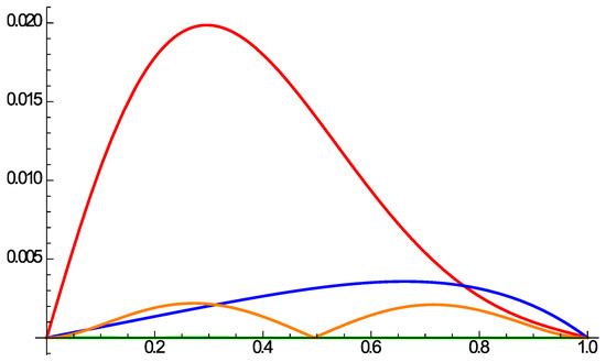
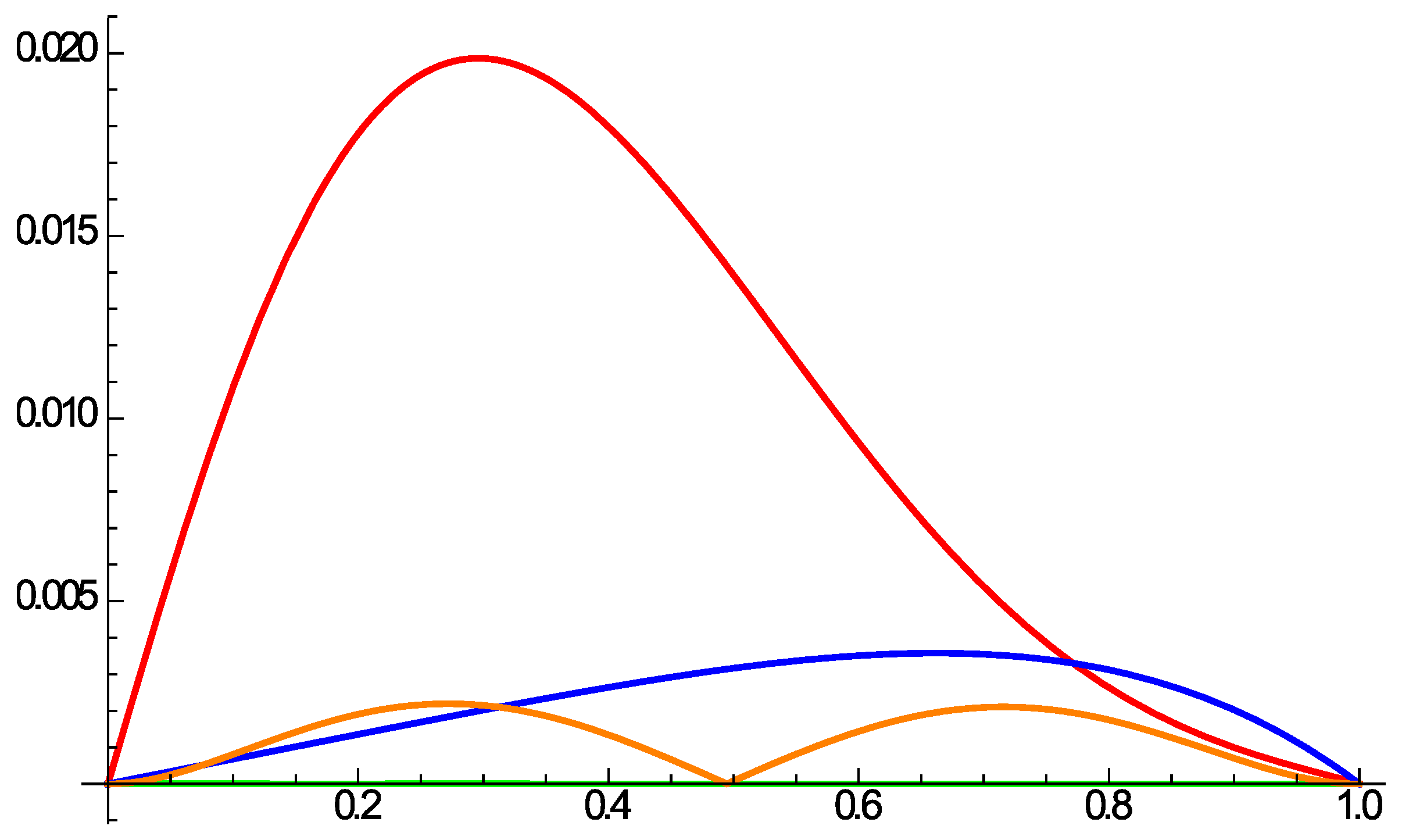
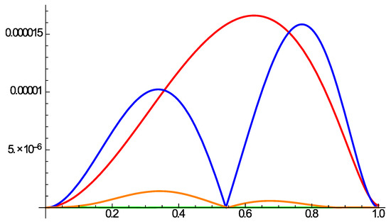
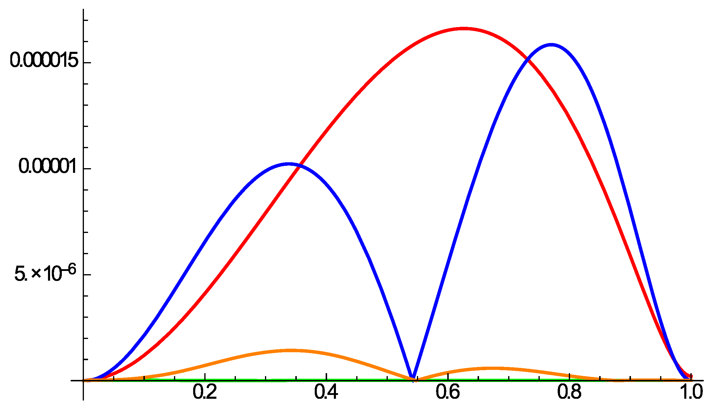
The comparison of these LSHPM solutions with the previous approximate solutions computed in [12] using HAM and DTM, and in [32] using PLSM, is presented in Figure 1 and Figure 2. Since no exact solutions are available, the comparison is done by means of computing the error relative to a fourth-order Runge–Kutta method numerical solution (i.e., the absolute errors are computed as the difference between our approximate solutions and the numerical solutions).

Figure 1. Comparison of absolute errors corresponding to the approximation from [12] $U_{DTM}$ (red curve), [10] $U_{HPM}$ 3 terms (blue curve), [32] $U_{PLSM}$ (orange curve), and our LSHPM approximation $U_{LSHPM}$ (green curve).

Figure 2. Comparison of absolute errors corresponding to the approximation from [12] $V_{DTM}$ (red curve), [10] $V_{HPM}$ 3 terms (blue curve), [32] $V_{PLSM}$ (orange curve), and our LSHPM approximation $V_{LSHPM}$ (green curve).

The comparison is further illustrated by Table 1 and Table 2, which includes the results obtained in [12], by means of the HAM and DTM, the results obtained in [32] by PLSM, and the results computed by classical HPM and by LSHPM. The comparison lead to the same conclusion: the approximate solutions obtained by LSHPM are more precise.

Table 1. Comparison of the absolute errors of the approximate solutions U in case $Re=1$ and $Ha=0$.

y	${\mathit{U}}_{\mathit{HAM}}$	${\mathit{U}}_{\mathit{DTM}}$	${\mathit{U}}_{\mathit{PLSM}}$	${\mathit{U}}_{\mathit{HPM}2\mathit{term}.}$	${\mathit{U}}_{\mathit{HPM}3\mathit{t}.}$	${\mathit{U}}_{\mathit{LSHPM}2\mathit{t}.}$	${\mathit{U}}_{\mathit{LSHPM}3\mathit{t}.}$
0.1	$9.04\times {10}^{-3}$	$1.08\times {10}^{-2}$	$8.06\times {10}^{-4}$	$4.45\times {10}^{-3}$	$6.77\times {10}^{-4}$	$8.61\times {10}^{-5}$	$3.68\times {10}^{-6}$
0.2	$1.77\times {10}^{-2}$	$1.77\times {10}^{-2}$	$1.90\times {10}^{-3}$	$9.08\times {10}^{-3}$	$1.35\times {10}^{-3}$	$8.00\times {10}^{-5}$	$1.56\times {10}^{-6}$
0.3	$2.71\times {10}^{-2}$	$1.98\times {10}^{-2}$	$2.14\times {10}^{-3}$	$1.37\times {10}^{-2}$	$2.01\times {10}^{-3}$	$4.18\times {10}^{-6}$	$3.41\times {10}^{-6}$
0.4	$3.45\times {10}^{-2}$	$1.79\times {10}^{-2}$	$1.34\times {10}^{-3}$	$1.78\times {10}^{-2}$	$2.64\times {10}^{-3}$	$9.71\times {10}^{-5}$	$9.99\times {10}^{-8}$
0.5	$3.73\times {10}^{-2}$	$1.39\times {10}^{-2}$	$8.14\times {10}^{-5}$	$2.10\times {10}^{-2}$	$3.16\times {10}^{-3}$	$1.29\times {10}^{-4}$	$2.42\times {10}^{-6}$
0.6	$3.46\times {10}^{-2}$	$9.33\times {10}^{-3}$	$1.43\times {10}^{-3}$	$2.24\times {10}^{-2}$	$3.50\times {10}^{-3}$	$7.69\times {10}^{-5}$	$1.22\times {10}^{-6}$
0.7	$2.77\times {10}^{-2}$	$5.39\times {10}^{-3}$	$2.09\times {10}^{-3}$	$2.15\times {10}^{-2}$	$3.54\times {10}^{-3}$	$2.59\times {10}^{-5}$	$9.10\times {10}^{-7}$
0.8	$1.87\times {10}^{-2}$	$2.63\times {10}^{-3}$	$1.74\times {10}^{-3}$	$1.78\times {10}^{-2}$	$3.12\times {10}^{-3}$	$9.63\times {10}^{-5}$	$7.61\times {10}^{-7}$
0.9	$9.27\times {10}^{-3}$	$9.33\times {10}^{-4}$	$6.99\times {10}^{-4}$	$1.07\times {10}^{-2}$	$2.02\times {10}^{-3}$	$6.71\times {10}^{-5}$	$4.05\times {10}^{-7}$

Table 2. Comparison of the absolute errors of the approximate solutions V in case $Re=1$ and $Ha=0$.

y	${\mathit{V}}_{\mathit{HAM}}$	${\mathit{V}}_{\mathit{DTM}}$	${\mathit{V}}_{\mathit{PLSM}}$	${\mathit{V}}_{\mathit{HPM}2\mathit{term}.}$	${\mathit{V}}_{\mathit{HPM}3\mathit{t}.}$	${\mathit{V}}_{\mathit{LSHPM}2\mathit{t}.}$	${\mathit{V}}_{\mathit{LSHPM}3\mathit{t}.}$
0.1	$2.21\times {10}^{-4}$	$1.19\times {10}^{-6}$	$1.48\times {10}^{-7}$	$2.25\times {10}^{-5}$	$2.13\times {10}^{-6}$	$1.41\times {10}^{-6}$	$2.20\times {10}^{-8}$
0.2	$5.75\times {10}^{-4}$	$4.10\times {10}^{-6}$	$7.17\times {10}^{-7}$	$1.14\times {10}^{-4}$	$6.55\times {10}^{-6}$	$1.21\times {10}^{-5}$	$9.78\times {10}^{-9}$
0.3	$6.47\times {10}^{-2}$	$7.91\times {10}^{-6}$	$1.34\times {10}^{-6}$	$2.83\times {10}^{-4}$	$9.89\times {10}^{-6}$	$3.20\times {10}^{-5}$	$4.69\times {10}^{-9}$
0.4	$3.03\times {10}^{-4}$	$1.17\times {10}^{-5}$	$1.26\times {10}^{-6}$	$4.95\times {10}^{-4}$	$9.25\times {10}^{-6}$	$5.07\times {10}^{-5}$	$1.40\times {10}^{-8}$
0.5	$2.63\times {10}^{-4}$	$1.49\times {10}^{-5}$	$4.45\times {10}^{-7}$	$6.84\times {10}^{-4}$	$3.56\times {10}^{-6}$	$5.66\times {10}^{-5}$	$1.53\times {10}^{-8}$
0.6	$7.02\times {10}^{-4}$	$1.65\times {10}^{-5}$	$3.80\times {10}^{-7}$	$7.75\times {10}^{-4}$	$5.54\times {10}^{-6}$	$4.58\times {10}^{-5}$	$1.84\times {10}^{-8}$
0.7	$7.62\times {10}^{-4}$	$1.59\times {10}^{-5}$	$5.63\times {10}^{-7}$	$7.12\times {10}^{-4}$	$1.37\times {10}^{-5}$	$2.53\times {10}^{-5}$	$1.67\times {10}^{-8}$
0.8	$4.73\times {10}^{-4}$	$1.23\times {10}^{-5}$	$2.24\times {10}^{-7}$	$4.87\times {10}^{-4}$	$1.54\times {10}^{-5}$	$7.48\times {10}^{-6}$	$1.46\times {10}^{-8}$
0.9	$1.25\times {10}^{-4}$	$5.88\times {10}^{-6}$	$2.11\times {10}^{-8}$	$1.80\times {10}^{-4}$	$8.05\times {10}^{-6}$	$2.77\times {10}^{-7}$	$1.41\times {10}^{-8}$

3.2. The Case $Re=1$ and $Ha=1$

In the case $Re=1$ and $Ha=1$, the influence of the magnetic field on the blood flow is non-negligible and the flow is weakly magnetic. The computations by LSHPM are similar to the ones in the previous case.

The approximations terms by HPM are:

• First-term approximations:

  $$\begin{array}{c}{U}_0\left(y\right)=1-y\\ V_0\left(y\right)=3y^2-2y^3\end{array}$$

  (26)
• Second-term approximations:

  $$\begin{array}{c}{U}_1\left(y\right)={\displaystyle \frac{y^5}{5}}-{\displaystyle \frac{3y^4}{4}}+{\displaystyle \frac{5y^3}{6}}+{\displaystyle \frac{y^2}{2}}-{\displaystyle \frac{107y}{60}}+1\\ V_1\left(y\right)={\displaystyle \frac{2y^7}{35}}-{\displaystyle \frac{y^6}{5}}+{\displaystyle \frac{y^5}{5}}+{\displaystyle \frac{y^4}{4}}-{\displaystyle \frac{181y^3}{70}}+{\displaystyle \frac{459y^2}{140}}\end{array}$$

  (27)
• Third-term approximations:

  $$\begin{array}{c}{U}_2\left(y\right)={\displaystyle \frac{2y^9}{315}}-{\displaystyle \frac{19y^8}{560}}+{\displaystyle \frac{9y^7}{140}}-{\displaystyle \frac{2y^6}{15}}+{\displaystyle \frac{2129y^5}{4200}}-{\displaystyle \frac{451y^4}{420}}+{\displaystyle \frac{401y^3}{504}}+{\displaystyle \frac{y^2}{2}}-{\displaystyle \frac{41129y}{25200}}+1\\ V_2\left(y\right)={\displaystyle \frac{4y^{11}}{5775}}-{\displaystyle \frac{2y^{10}}{525}}+{\displaystyle \frac{y^9}{140}}-{\displaystyle \frac{9y^8}{560}}+{\displaystyle \frac{1507y^7}{14700}}-{\displaystyle \frac{1129y^6}{4200}}+{\displaystyle \frac{317y^5}{1400}}+{\displaystyle \frac{153y^4}{560}}\\ -{\displaystyle \frac{838379y^3}{323400}}+{\displaystyle \frac{352623y^2}{107800}}\end{array}$$

  (28)

The corresponding solutions obtained by using LSHPM are:

• Second-term approximations:
  $\tilde{U}\left(y\right)=0.24252310472551437387y^5-0.79607170987751279666y^4$
  $+0.70039529434560076978y^3+0.51680281524640722276y^2$
  $-1.6636495044400095698y+1$
  $\tilde{V}\left(y\right)=0.058199385875154810585y^7-0.20176414373359385855y^6$
  $+0.17947791112252870094y^5+0.28462933749944678084y^4-2.5916327628078782832y^3$
  $+3.2710902720443418494y^2$
• Third-term approximations:
  $\tilde{U}\left(y\right)=-0.039570918805227895983y^9+0.18039801278862870509y^8$
  $-0.33738809541609613996y^7+0.25556139173308396128y^6+0.28898499486097221037y^5$
  $-0.98687905924276726841y^4+0.80192640217575596712y^3+0.50063075107844706510y^2$
  $-1.6636634791727966046y+1$
  $\tilde{V}\left(y\right)=0.00070249628967946626576y^{11}-0.0034005002946346048030y^{10}$
  $+0.0063398061612668565765y^9-0.017261143110682215908y^8$
  $+0.10727677845680360313y^7-0.27266199870132195652y^6+0.22694957760601929024y^5$
  $+0.27260900187074289280y^4-2.5917328827530869045y^3+3.2711788644752135727y^2$

Again, the comparisons included in Table 3 and Table 4 allow us the reach the same conclusion as in the previous case, namely that the approximations obtained by LSHPM are more accurate than the previous ones by other methods.

Table 3. Comparison of the absolute errors of the approximate solutions for U for the case $Re=1$ and $Ha=1$.

y	${\mathit{U}}_{\mathit{HAM}}$	${\mathit{U}}_{\mathit{DTM}}$	${\mathit{U}}_{\mathit{PLSM}}$	${\mathit{U}}_{\mathit{HPM}2\mathit{term}.}$	${\mathit{U}}_{\mathit{HPM}3\mathit{t}.}$	${\mathit{U}}_{\mathit{LSHPM}2\mathit{t}.}$	${\mathit{U}}_{\mathit{LSHPM}3\mathit{t}.}$
0.1	$1.19\times {10}^{-2}$	$3.18\times {10}^{-2}$	$8.22\times {10}^{-5}$	$1.19\times {10}^{-2}$	$3.13\times {10}^{-3}$	$8.03\times {10}^{-5}$	$4.19\times {10}^{-7}$
0.2	$1.59\times {10}^{-2}$	$5.15\times {10}^{-2}$	$1.17\times {10}^{-4}$	$2.33\times {10}^{-2}$	$6.14\times {10}^{-3}$	$1.14\times {10}^{-4}$	$1.14\times {10}^{-6}$
0.3	$1.25\times {10}^{-2}$	$5.95\times {10}^{-2}$	$3.15\times {10}^{-5}$	$3.35\times {10}^{-2}$	$8.85\times {10}^{-3}$	$2.72\times {10}^{-5}$	$1.41\times {10}^{-7}$
0.4	$5.92\times {10}^{-3}$	$5.84\times {10}^{-2}$	$9.22\times {10}^{-5}$	$4.14\times {10}^{-2}$	$1.10\times {10}^{-2}$	$9.64\times {10}^{-5}$	$1.32\times {10}^{-6}$
0.5	$1.62\times {10}^{-4}$	$5.14\times {10}^{-2}$	$1.48\times {10}^{-4}$	$4.60\times {10}^{-2}$	$1.25\times {10}^{-2}$	$1.52\times {10}^{-4}$	$3.46\times {10}^{-7}$
0.6	$2.79\times {10}^{-3}$	$4.11\times {10}^{-2}$	$9.29\times {10}^{-5}$	$4.65\times {10}^{-2}$	$1.29\times {10}^{-2}$	$9.57\times {10}^{-5}$	$1.10\times {10}^{-6}$
0.7	$3.20\times {10}^{-3}$	$2.99\times {10}^{-2}$	$3.03\times {10}^{-5}$	$4.24\times {10}^{-2}$	$1.22\times {10}^{-2}$	$2.86\times {10}^{-5}$	$3.63\times {10}^{-7}$
0.8	$2.34\times {10}^{-3}$	$1.92\times {10}^{-2}$	$1.16\times {10}^{-4}$	$3.33\times {10}^{-2}$	$9.21\times {10}^{-3}$	$1.15\times {10}^{-4}$	$7.95\times {10}^{-7}$
0.9	$1.21\times {10}^{-3}$	$9.05\times {10}^{-3}$	$8.04\times {10}^{-5}$	$1.92\times {10}^{-2}$	$5.92\times {10}^{-3}$	$8.01\times {10}^{-5}$	$1.05\times {10}^{-7}$

Table 4. Comparison of the absolute errors of the approximate solutions for V for the case $Re=1$ and $Ha=1$.

y	${\mathit{V}}_{\mathit{HAM}}$	${\mathit{V}}_{\mathit{DTM}}$	${\mathit{V}}_{\mathit{PLSM}}$	${\mathit{V}}_{\mathit{HPM}2\mathit{term}.}$	${\mathit{V}}_{\mathit{HPM}3\mathit{t}.}$	${\mathit{V}}_{\mathit{LSHPM}2\mathit{t}.}$	${\mathit{V}}_{\mathit{LSHPM}3\mathit{t}.}$
0.1	$4.90\times {10}^{-4}$	$2.70\times {10}^{-4}$	$3.06\times {10}^{-8}$	$7.74\times {10}^{-5}$	$1.53\times {10}^{-6}$	$1.14\times {10}^{-8}$	$1.91\times {10}^{-8}$
0.2	$1.15\times {10}^{-3}$	$5.83\times {10}^{-4}$	$8.27\times {10}^{-8}$	$3.03\times {10}^{-4}$	$8.01\times {10}^{-6}$	$5.24\times {10}^{-6}$	$7.27\times {10}^{-9}$
0.3	$1.19\times {10}^{-3}$	$5.51\times {10}^{-4}$	$1.37\times {10}^{-7}$	$6.22\times {10}^{-4}$	$2.06\times {10}^{-6}$	$1.87\times {10}^{-5}$	$4.18\times {10}^{-10}$
0.4	$4.36\times {10}^{-4}$	$1.45\times {10}^{-4}$	$1.04\times {10}^{-7}$	$9.38\times {10}^{-4}$	$3.79\times {10}^{-6}$	$3.38\times {10}^{-5}$	$3.16\times {10}^{-9}$
0.5	$7.25\times {10}^{-4}$	$4.47\times {10}^{-4}$	$1.51\times {10}^{-8}$	$1.14\times {10}^{-3}$	$5.51\times {10}^{-6}$	$4.05\times {10}^{-5}$	$1.35\times {10}^{-9}$
0.6	$1.66\times {10}^{-3}$	$9.52\times {10}^{-4}$	$9.11\times {10}^{-8}$	$1.16\times {10}^{-3}$	$6.56\times {10}^{-6}$	$3.41\times {10}^{-5}$	$3.91\times {10}^{-10}$
0.7	$1.90\times {10}^{-3}$	$1.12\times {10}^{-3}$	$6.89\times {10}^{-8}$	$9.70\times {10}^{-4}$	$6.30\times {10}^{-5}$	$1.91\times {10}^{-5}$	$1.24\times {10}^{-9}$
0.8	$1.35\times {10}^{-3}$	$8.72\times {10}^{-4}$	$1.55\times {10}^{-8}$	$6.05\times {10}^{-4}$	$4.48\times {10}^{-5}$	$5.55\times {10}^{-6}$	$7.28\times {10}^{-10}$
0.9	$4.73\times {10}^{-4}$	$3.42\times {10}^{-4}$	$6.71\times {10}^{-10}$	$2.04\times {10}^{-4}$	$1.71\times {10}^{-6}$	$1.06\times {10}^{-7}$	$3.35\times {10}^{-9}$

We mention the fact that we computed approximations for a wide range of values of the parameters $Re$ and $Ha$, and the above conclusions remained valid for all of the computed solutions.

4. Discussion of the Results

As we mention in the previous section, we computed approximations for a wide range of values of the parameters $Re$ and $Ha$, and the conclusions of our study are in very good agreement with previous ones included in [12,33,34,35] and other studies. This is to be expected because, even though our approximations are much more precise than the ones included in the previous studies, the overall phenomena described by the solutions are obviously the same. In the following, we will briefly summarize the results of the study.

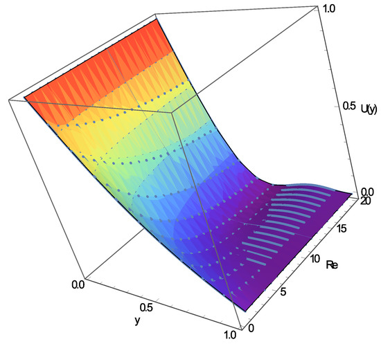
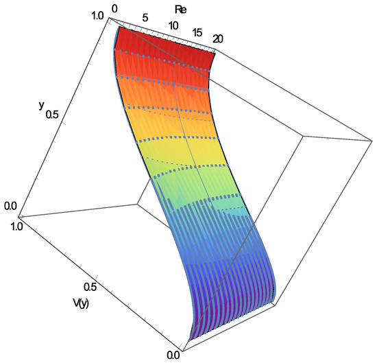
The first results are related to the influence of the Reynolds number on the velocities U and V, when the value of the Hartmann number is fixed. We were able to draw similar conclusions for both cases studied in [12] (the non-conducting case $Ha=0$ and the weakly magnetic flow case $Ha=1$). The consequences of any increase of the Reynolds number are a modest increase to the $V\left(y\right)$ component of the velocity of the blood flow, and a major decrease of the $U\left(y\right)$ component. The effect of this phenomenon is a major deceleration of the blood velocity in the x-direction. For the case $Ha=0$, these conclusions are illustrated by the Figure 3 and Figure 4, while for the case $Ha=1$ (and, actually, for any other value of $Ha$ on its nominal interval [0, 2]), the figures look very similar.

Figure 3. The effect of the increase of $Re$ on U for the case $Ha=0$—three dimensional plot.

Figure 4. The effect of the increase of $Re$ on V for the case $Ha=0$—three dimensional plot.

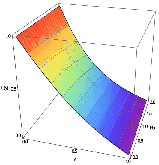
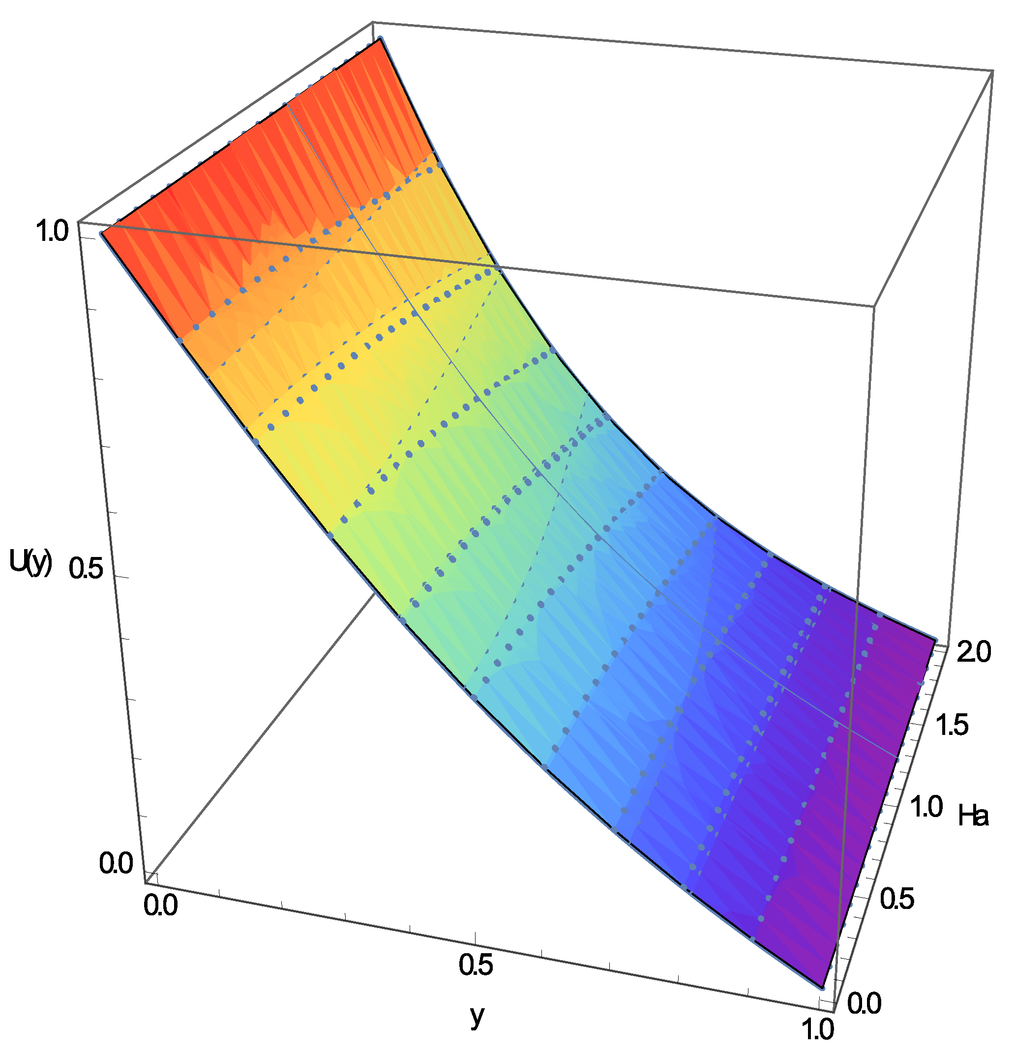
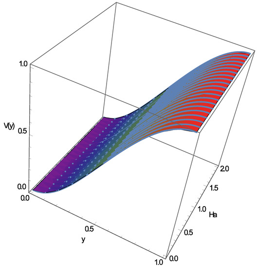
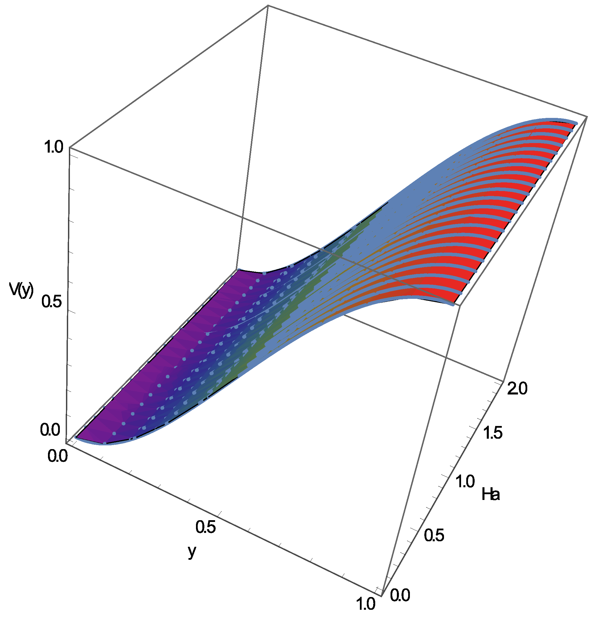
The next study item is the influence of the Hartmann number on the velocities U and V for fixed values of the Reynolds number. Because the magnetic field is applied in the y-direction only, there is no visible influence of the increase of the $Ha$ $V\left(y\right)$ component of the blood velocity while there is a decrease of the $U\left(y\right)$ component, as expected. These conclusions are illustrated for $Re=1$ in Figure 5 and Figure 6 (again, we mention that for any values of the Reynolds number on its nominal interval [1, 20], the figures are similar).

Figure 5. The effect of the increase of $Ha$ on U for the case $Re=1$—three dimensional plot.

Figure 6. The effect of the increase of $Ha$ on V for the case $Re=1$—three dimensional plot.

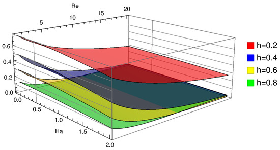
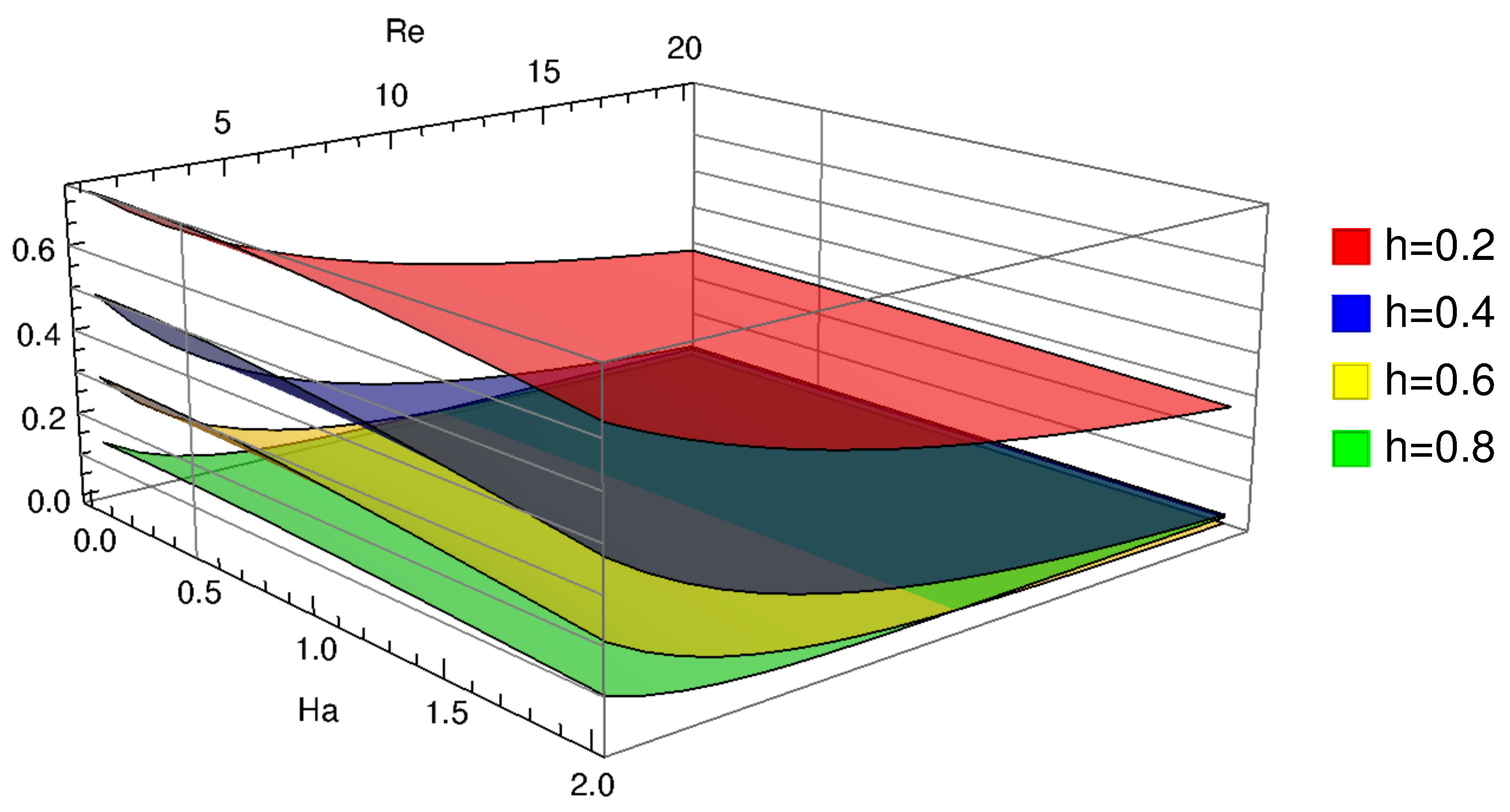
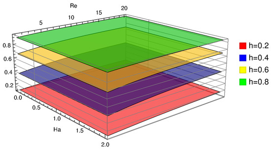
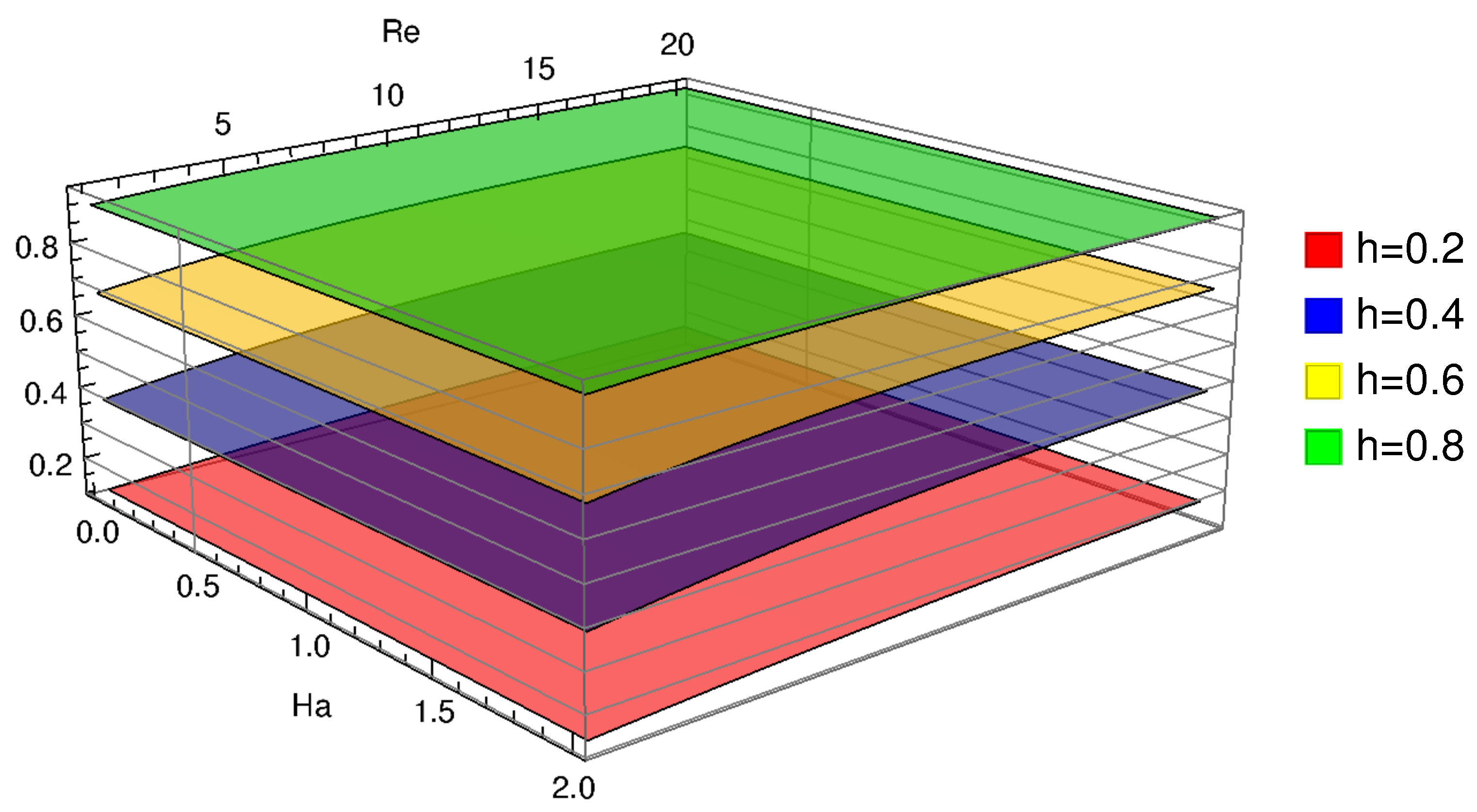
In the last part of the study, we investigated the merged impact of $Re$ and $Ha$ on $U\left(y\right)$ and $V\left(y\right)$, impact highlighted in the Figure 7 and Figure 8 for $y=0.2$ (red surface), $y=0.4$ (blue surface), $y=0.6$ (yellow surface) and $y=0.8$ (green surface).

Figure 7. The combined influence of $Re$ and $Ha$ on U. The red surface corresponds to $y=0.2$, the blue surface to $y=0.4$, the yellow surface to $y=0.6$ and the green one to $y=0.8$.

Figure 8. The combined influence of $Re$ and $Ha$ on V. The red surface corresponds to $y=0.2$, the blue surface to $y=0.4$, the yellow surface to $y=0.6$, and the green one to $y=0.8$.

Figure 7 is a good synthesis of the research done on the impact of $Re$ and $Ha$ on a replicated blood flow in a semi-porous channel, as it is obvious that the increase in both $Re$ and $Ha$ conduct to the reduction of $U\left(y\right)$. At the same time, Figure 8 gives new insight regarding the interplay between the impact of $Re$ and $Ha$ on the blood flow velocity in the y-direction, particularly the fact that the decelerative consequence of the increase of $Ha$ greatly depends on $Re$. This effect is greater for reduced values of $Re$ and, as a result, in situations where, due to practical discussions, a strong suction at the upper wall ( defined by a large value of $Re$) cannot be achieved, a decrease of blood flow velocity can be achieved by boosting the intensity of the magnetic field applied. Even if it is practically possible, an increase of the suction at the upper wall is apparently the preferable method for reducing the flow, since the effect of the increase of Re seems to be considerably greater than the effect of the increase of Ha. Furthermore, if the value of the Reynolds number is large, the consequences of the increase of the Hartmann number is small.

5. Conclusions

The least squares homotopy perturbation method is introduced as a straightforward and very accurate method to compute analytically approximate solutions for systems of ordinary differential equations.

The method was employed for a system of equations modeling the blood flow through a blood vessel under the action of a magnetic field. The comparison with approximate solutions computed by using well-known methods, such as the homotopy analysis method, the differential transform method and the homotopy perturbation method, clearly illustrate the precision of our method.

References

- Bota, C.; Caruntu, B. Approximate analytical solutions of nonlinear differential equations using the Least Squares Homotopy Perturbation Method. J. Math. Anal. Appl. 2017, 448, 401–408. [Google Scholar] [CrossRef] [Scilit]
- Bota, C.; Caruntu, B.; Lazureanu, C. The Least Squares Homotopy Perturbation Method for boundary value problems. Appl. Comput. Math. 2017, 16, 39–47. [Google Scholar]
- Qayyum, M.; Oscar, I. Least Square Homotopy Perturbation Method for Ordinary Differential Equations. J. Math. 2021, 2021, 7059194. [Google Scholar] [CrossRef] [Scilit]
- Thabet, H.; Kendre, S. Modified least squares homotopy perturbation method for solving fractional partial differential equations. Malaya J. Mat. 2018, 6, 420–427. [Google Scholar] [CrossRef] [Scilit]
- Kumar, R.; Koundal, R.; Shehzad, S.A. Generalized least square homotopy perturbation solution of fractional telegraph equations. Comput. Appl. Math. 2019, 38, 184. [Google Scholar] [CrossRef] [Scilit]
- Zhang, J.; Wei, Z.; Li, L.; Zhou, C. Least-Squares Residual Power Series Method for the Time-Fractional Differential Equations. Complexity 2019, 2019, 6159024. [Google Scholar] [CrossRef] [Scilit]
- Das, P.; Rana, S. Theoretical prospects of fractional order weakly singular Volterra Integro differential equations and their approximations with convergence analysis. Math. Methods Appl. Sci. 2021, 44, 9419–9440. [Google Scholar] [CrossRef] [Scilit]
- Kumar, R.; Koundal, R.; Shehzad, S.A. Modified homotopy perturbation approach for the system of fractional partial differential equations: A utility of fractional Wronskian. Math. Methods Appl. Sci. 2022, 45, 809–826. [Google Scholar] [CrossRef] [Scilit]
- He, J.H. Homotopy perturbation technique. Comput. Methods Appl. Mech. Eng. 1999, 178, 257–262. [Google Scholar] [CrossRef] [Scilit]
- He, J.H. Application of homotopy perturbation method to nonlinear wave equations. Chaos Solitons Fractals 2005, 26, 695–700. [Google Scholar] [CrossRef] [Scilit]
- He, J.H. Variational iteration method, a kind of nonlinear analytical technique. Some examples. Int. J. Non-Linear Mech. 1999, 34, 699–708. [Google Scholar] [CrossRef] [Scilit]
- Parsa, A.B.; Rashidi, M.M.; Beg, O.A.; Sardi, S.M. Semi-computational simulation of magneto-hemodynamic flow in a semi-porous channel using optimal homotopy and differential transform methods. Comput. Biol. Med. 2013, 43, 1142–1153. [Google Scholar] [CrossRef] [Scilit] [PubMed]
- Adomian, G.A. Review of the decomposition method in applied mathematics. J. Math. Anal. Appl. 1998, 135, 501–544. [Google Scholar] [CrossRef] [Scilit]
- Marinca, V.; Herisanu, N.; Bota, C. An optimal homotopy asymptotic method applied to the steady flow of a fourth-grade fluid past a porous plate. Appl. Math. Lett. 2009, 22, 245–251. [Google Scholar] [CrossRef] [Scilit]
- Srivastava, V.P. A Theoretical Model for Blood Flow in Small Vessels. Int. J. Appl. Appl. Math. 2007, 2, 51–65. [Google Scholar]
- Wang, C.Y.; Bassingthwaighte, J.B. Blood Flow in Small Curved Tubes. J. Biomech. Eng. 2003, 125, 910–913. [Google Scholar] [CrossRef] [Scilit] [PubMed]
- Bali, R.; Awasthi, U. Mathematical model of Blood Flow in Small Blood Vessel in the Presence of Magnetic Field. Appl. Math. 2001, 2, 264–269. [Google Scholar] [CrossRef]
- Yamamoto, T.; Nagayama, Y.; Tamura, M. A blood-oxygenation-dependent increase in blood viscosity due to a static magnetic field. Phys. Med. Biol. 2004, 49, 3267. [Google Scholar] [CrossRef] [Scilit] [PubMed]
- Alshare, A.; Tashtoush, B.; El-Khalil, H.H. Computational Modeling of Non-Newtonian Blood Flow Through Stenosed Arteries in the Presence of Magnetic Field. J. Biomech. Eng. 2013, 135, 1145–1153. [Google Scholar] [CrossRef] [Scilit]
- Weng, H.C. Hydrodynamic Modeling of Targeted Magnetic-Particle Delivery in a Blood Vessel. J. Biomech. Eng. 2013, 135, 034504. [Google Scholar] [CrossRef] [Scilit] [PubMed]
- Mekheimer, K.S. Peristaltic flow of blood under effect of a magnetic field in a non-uniform channels. Appl. Math. Comput. 2004, 153, 763–777. [Google Scholar] [CrossRef] [Scilit]
- Tenforde, T.S. Magnetically induced electric fields and currents in the circulatory system. Prog. Biophys. Mol. Biol. 2005, 87, 279–288. [Google Scholar] [CrossRef] [Scilit] [PubMed]
- Bhatti, M.M.; Zeeshan, A.; Bashir, F.; Sait, S.M.; Ellahi, R. Sinusoidal motion of small particles through a Darcy-Brinkman-Forchheimer microchannel filled with non-Newtonian fluid under electro-osmotic forces. J. Taibah Univ. Sci. 2021, 15, 514–529. [Google Scholar] [CrossRef] [Scilit]
- Rostami, S.; Ellahi, R.; Oztop, H.F.; Goldanlou, A.S. A study on the effect of magnetic field and the sinusoidal boundary condition on free convective heat transfer of non-Newtonian power-law fluid in a square enclosure with two constant-temperature obstacles using lattice Boltzmann method. J. Therm. Anal. Calorim. 2021, 144, 2557–2573. [Google Scholar] [CrossRef] [Scilit]
- Khan, A.S.; Xu, H.Y.; Khan, W. Magnetohydrodynamic Hybrid Nanofluid Flow Past an Exponentially Stretching Sheet with Slip Conditions. Mathematics 2021, 9, 3291. [Google Scholar] [CrossRef] [Scilit]
- Rehman, A.; Salleh, Z. Influence of Marangoni Convection on Magnetohydrodynamic Viscous Dissipation and Heat Transfer on Hybrid Nanofluids in a Rotating System among Two Surfaces. Mathematics 2021, 9, 2242. [Google Scholar] [CrossRef] [Scilit]
- Ali, B.; Naqvi, R.A.; Haider, A.; Hussain, D.; Hussain, S. Finite Element Study of MHD Impacts on the Rotating Flow of Casson Nanofluid with the Double Diffusion Cattaneo—Christov Heat Flux Model. Mathematics 2020, 8, 1555. [Google Scholar] [CrossRef] [Scilit]
- Ryu, J.; Hu, X.; Shadden, S.C. A Coupled Lumped-Parameter and Distributed Network Model for Cerebral Pulse-Wave Hemodynamics. J. Biomech. Eng. 2015, 137, 101009. [Google Scholar] [CrossRef] [Scilit]
- Srinivasacharya, D.; Rao, G.M. Mathematical model for blood flow through a bifurcated artery using couple stress fluid. Math. Biosci. 2016, 278, 37–47. [Google Scholar] [CrossRef] [Scilit]
- Sinha, A. MHD flow and heat transfer of a third order fluid in a porous channel with stretching wall: Application to hemodynamics. Alex. Eng. J. 2015, 54, 1243–1252. [Google Scholar] [CrossRef] [Scilit]
- Zaman, A.; Ali, N.; Sajid, M. Numerical simulation of pulsatile flow of blood in a porous-saturated overlapping stenosed artery. Math. Comput. Simul. 2017, 134, 1–16. [Google Scholar] [CrossRef] [Scilit]
- Caruntu, B.; Bota, C.; Bundau, O. Analytical simulation of magneto-hemodynamic flow in a semi-porous channel using the Polynomial Least Squares Method. ITM Web Conf. 2019, 29, 1–13. [Google Scholar] [CrossRef] [Scilit]
- Skalak, F.M.; Wang, C.Y. On the non-unique solutions of laminar flow through a porous tube or channel. SIAM J. Appl. Math. 1978, 34, 535–544. [Google Scholar] [CrossRef] [Scilit]
- Quaile, J.P.; Levy, E.K. Laminar flow in a porous tube with suction. Int. J. Heat Mass Transf. 1975, 97, 223–243. [Google Scholar] [CrossRef] [Scilit]
- Evans, E.A.; Skalak, R. Mechanics and Thermodynamics of Biomembranes. In Elsevier Biomedical; Hue, L., Van de Werve, G., Eds.; Elsevier Biomedical: Amsterdam, NY, USA, 1981; 464p. [Google Scholar]
Publisher’s Note: MDPI stays neutral with regard to jurisdictional claims in published maps and institutional affiliations. |
© 2022 by the authors. Licensee MDPI, Basel, Switzerland. This article is an open access article distributed under the terms and conditions of the Creative Commons Attribution (CC BY) license (https://creativecommons.org/licenses/by/4.0/).