Numerical Analysis of Fourier Finite Volume Element Method for Dirichlet Boundary Optimal Control Problems Governed by Elliptic PDEs on Complex Connected Domains

Abstract

In this research, we investigate an optimal control problem governed by elliptic PDEs with Dirichlet boundary conditions on complex connected domains, which can be utilized to model the cooling process of concrete dam pouring. A new convergence result for two-dimensional Dirichlet boundary control is proven with the Fourier finite volume element method. The Lagrange multiplier approach is employed to find the optimality systems of the Dirichlet boundary optimal control problem. The discrete optimal control problem is then obtained by applying the Fourier finite volume element method based on Galerkin variational formulation for optimality systems, that is, using Fourier expansion in the azimuthal direction and the finite volume element method in the radial direction, respectively. In this way, the original two-dimensional problem is reduced to a sequence of one-dimensional problems, with the Dirichlet boundary acting as an interval endpoint at which a quadratic interpolation scheme can be implemented. The convergence order of state, adjoint state, and Dirichlet boundary control are therefore proved. The effectiveness of the method is demonstrated numerically, and numerical data is provided to support the theoretical analysis.

1. Introduction

Partial differential equations are commonly used to describe two-dimensional plane stable field equations like steady concentration distributions, stable temperature distributions, electrostatic field equations, steady current field equations without rotation, and steady flow equations without rotation [1,2,3,4]. The optimal control problems governed by elliptic partial differential equations also play an important role in physical engineering, biological engineering, and social sciences areas, see [5,6,7,8,9,10]. Since the 1970s, the numerical approximation methods for optimal control problems have all received increasing attention. The main research methods are the finite difference method [11], finite element method [12,13,14,15], finite volume element method [16], and spectral method [17,18,19].

The optimal control problem [6,7] is a mathematical problem in which the minimum value of an objective function is determined under differential equation constraints. Finding a numerical solution is essential because it is challenging to find an analytical solution to a problem of this nature. In this paper, we look at a Dirichlet boundary optimal control problem on a complex connected domain that is governed by elliptic equations. The form is as follows:

$$\underset{u\in U_{ad}}{min}J\left(y,u\right):=\frac{1}{2}{∥y-y_d∥}_{L^2\left(\Omega \right)}^2+\frac{\alpha }{2}{∥u∥}_{L^2\left(\partial {\Omega }_1\right)}^2,$$

(1)

subject to

$$\begin{array}{c}\hfill \left\{\begin{array}{cc}-\Delta y=f,\hfill & \mathrm{in}\Omega ,\hfill \\ y=u,\hfill & \mathrm{on}\partial {\Omega }_1,\hfill \\ \frac{\partial y}{\partial n_2}=0,\hfill & \mathrm{on}\partial {\Omega }_2.\hfill \end{array}\right.\end{array}$$

(2)

The set $\Omega \subset R^2$ denotes a bounded complex connected domain with boundary $\Gamma =\partial {\Omega }_1\cup \partial {\Omega }_2$. Equation (2) is a state equation, y is the state variable, $u\in \partial {\Omega }_1$ is the Dirichlet boundary control variable, $\alpha >0$ is a regularization parameter, and $y_d\in H^1\left(\Omega \right)$, $f\in H^1\left(\Omega \right)$. $n_2$ is the outer unit normal of the boundary $\partial {\Omega }_2$. $U_{ad}$ is the admissible control set which is assumed to be of box type

$$u\in U_{ad}:=\left\{u\in H^{1/2}\left(\partial {\Omega }_1\right):u_a\le u\le u_b\right\}$$

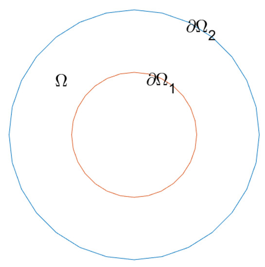
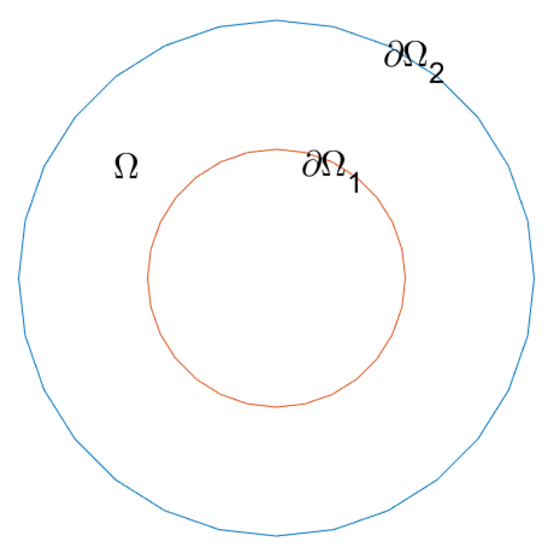
with $u_a<u_b$ denoting constants. The domain is shown as Figure 1.

Figure 1. Domain.

This optimal Dirichlet boundary control problem can be used to describe the cooling process of concrete dam pouring [20]. $\partial {\Omega }_1$ is the pipe boundary on which the cold water enters and is therefore a Dirichlet boundary control condition. $\Omega$ indicates the region where the cold water acts, and $y_d$ is the ideal state; the goal is to control the temperature of the cold water so that the temperature $y\in \Omega$ is infinitely close to $y_d$. Note that there is no heat exchange on $\partial {\Omega }_2$ and hence a homogeneous Neumann boundary condition.

Dirichlet boundary control problems are more challenging than Neumann control or distributed control problems in general, both theoretically and numerically. However, the Dirichlet situation is attracting an increasing number of researchers. For example, the semilinear elliptic Dirichlet boundary control problem with pointwise control constraints in a convex, polygonal, open domain is studied and the $1-1/p$ convergence order of control is derived in [21]. The authors in [22] considered Dirichlet boundary control problems posed on smooth domains and obtained that the error order of control is ${h\left|lnh\right|}^{1/2}$. Based on a mixed variation scheme, the authors in [23] used a mixed finite element method to approximate the optimal control problem posed on both polygonal and general smooth domains. The authors in [24] used local mesh refinement toward the boundary by standard finite element discretizations and arrived second-order convergence. [25] also derived second-order convergence for elliptic Dirichlet boundary control but in finite dimensional control space. Numerical analysis for elliptic control problems can be found in [21,26,27,28]. For more details, one may refer to [12,29,30] and the references therein. In addition, for finite element approximations of distributed and Neumann boundary optimal control problems one can see [31,32,33,34,35], and for other numerical methods, one may refer to [36,37,38,39].

The finite volume element method (FVEM) is a discretization technique for partial differential equations. It is widely employed in the numerical approximation of some problems for partial differential equations because of its local conservative property and other appealing properties, such as robustness with unstructured meshes. For instance, the authors in [40] analyzed the spatially semidiscrete piecewise linear finite volume element method for parabolic equations in a convex polygonal domain in the plane. Two-grid finite volume element discretization techniques were presented for the two-dimensional second-order nonself-adjoint and indefinite linear elliptic problems and the two-dimensional second-order nonlinear elliptic problems in [41]. A priori error estimates for a semidiscrete piecewise linear finite volume element approximation to a second-order wave equation in a two-dimensional convex polygonal domain is discussed in [42]. More applications of the finite volume element method can be referred to [43,44,45,46,47,48,49,50] and the references therein.

The combination of the finite volume element method with other numerical methods can generate competitive numerical methods for solving partial differential equation problems. For example, an immersed finite volume element method was used to solve the elliptic interface problems in [51]. A one-parameter family of discontinuous Galerkin finite volume element methods was applied to approximate the solution of a class of second-order linear elliptic problems in [52]. The Fourier finite volume element method was employed to study two-dimensional quasigeostrophic equations on a sphere in [53]. The authors in [54] utilized the Fourier finite volume element method to give the numerical experiments of two classes of Dirichlet and distributed optimal control problems driven by elliptic PDEs on complex connected domains. The main concept behind the Fourier finite volume element approach is to employ the finite volume element method in the radial direction while applying the Fourier expansion in the azimuthal direction. In the radial direction, choose linear finite element and piecewise constant function spaces for the trial and test function spaces, respectively. The control for the variational inequality is generated employing a variational discretization technique (see [55]). As a result, the two-dimensional optimal control problem can be simplified to a sequence of one-dimension problems. A desired result can be obtained by this procedure.

Generally, the Dirichlet boundary optimal control problem is typically challenging to achieve a high order in two-dimensional environments. The purpose of this article is to provide a related theoretical explanation of this problem, as a prior work on numerical simulation [54] demonstrates that the Fourier finite element approach can reduce the error order of Dirichlet boundary control on complex connected domains. In addition, it is worth noting that, in contrast to [25], the Dirichlet boundary control space in this work possesses infinite dimensions.

To the best of our knowledge, this is the first study to estimate the convergence order of the Dirichlet boundary control problem using the Fourier finite volume element approach on complex connected domains. The error of Dirichlet boundary control consists of two parts: The Fourier truncation error and the one-dimensional finite volume element error. The Fourier finite volume element approach is applied to reduce a two-dimensional optimal control problem to a group of one-dimensional problems, with the Dirichlet boundary acting as an interval endpoint at which a quadratic interpolation scheme can be implemented so that Dirichlet boundary control can be reached to higher order convergence. It is pointed out here that this proving method can also be extended to the parabolic problem.

The outline for this paper is provided below. In Section 2, we deduce the optimal control problem and corresponding optimality conditions. In order to solve the elliptic problem, the Fourier finite volume element method is introduced in Section 3. In Section 4, the Fourier finite volume element method is used to demonstrate the convergence order of the Dirichlet boundary control. A few examples are given in Section 5 to help illustrate the theoretical analysis. Some recommendations are made toward the end of Section 6.

2. Optimality System

For $m\ge 0$ and $1\le s\le \infty$, applying the standard notation $W^{m,s}$ for Sobolev space on $\Omega$ with $\left|\right|·{\left|\right|}_{m,s,\Omega }$ and denoting by $H^m\left(\Omega \right)$ with norm $\left|\right|·{\left|\right|}_{m,\Omega }$ and seminorm ${|·|}_{m,\Omega }$ for $s=2$. That is,

$$W^{m,s}\left(\Omega \right):=\left\{v\in L^s\left(\Omega \right),|D^{\alpha }v\in L^s\left(\Omega \right),\forall \alpha \in {\mathbb{Z}}_{+}^n,\left|\alpha \right|\le m\right\},$$

and

$${∥v∥}_{W^{m,s}\left(\Omega \right)}={\left(\sum _{\left|\alpha \right|\le m}{\int }_{\Omega }{\left|D^{\alpha }v\right|}^{s}dx\right)}^{\frac{1}{\mathrm{s}}},{\left|v\right|}_{W^{m,s}\left(\Omega \right)}={\left(\sum _{\left|\alpha \right|=m}{\int }_{\Omega }{\left|D^{\alpha }v\right|}^{s}dx\right)}^{\frac{1}{\mathrm{s}}},$$

where $D^{\alpha }v$ denotes the $\alpha$-th order weak derivative of v.

We use $\left(·,·\right)$ for the $L^2\left(\Omega \right)$-inner product, ${⟨·,·⟩}_{\partial {\Omega }_1}$ for the $L^2\left(\partial {\Omega }_1\right)$-inner product, ${\left(·,·\right)}_Q$ for the $L^2\left(Q\right)$-inner product, ${⟨·,·⟩}_{{\Gamma }_1}$ for the $L^2\left({\Gamma }_1\right)$-inner product, and ${\left(·,·\right)}_I$ for the $L^2\left(I\right)$-inner product.

Let $Y:=\left\{v\in H^1\left(\Omega \right){,v|}_{\partial {\Omega }_1}=u\right\}$ and $V:=\left\{v\in H^1\left(\Omega \right){,v|}_{\partial {\Omega }_1}=0\right\}$; the weak formulation of the state Equation (2) reads: find $y\in Y$ such that

$$a\left(y,v\right)=\left(f,v\right),\forall v\in V,$$

(3)

where the bilinear form $a\left(·,·\right)$ is given by

$$a\left(y,v\right)={\int }_{\Omega }\nabla y·\nabla vdx.$$

Then, the optimal control problem (1) and (2) can be described as: Find $\left(y,u\right)\in Y\times U_{ad}$

$$\begin{array}{c}\hfill \left(P\right)\left\{\begin{array}{c}\underset{u\in U_{ad}}{min}J\left(y,u\right):=\frac{1}{2}{∥y-y_d∥}_{L^2\left(\Omega \right)}^2+\frac{\alpha }{2}{∥u∥}_{L^2\left(\partial {\Omega }_1\right)}^2,\hfill \\ s.t.a\left(y,v\right)=\left(f,v\right),\forall v\in V.\hfill \end{array}\right.\end{array}$$

(4)

Suppose that $\left(\overline{y},\overline{u}\right)$ is the optimal solution. This is due to the fact that the control problem is strictly convex and satisfies the existence and uniqueness requirements of the solution in the constrained state Equation (2). Then, using the Lagrange multiplier method [5,7] to construct Lagrange function

$$L\left(y,u,p\right)=J\left(y,u\right)-{\int }_{\Omega }\left(-\Delta y-f\right)pdx-{\int }_{\partial {\Omega }_1}\left(y-u\right)pds-{\int }_{\partial {\Omega }_2}\left(\frac{\partial y}{\partial n_2}\right)pds.$$

We take the  Fréchet  derivative with respect to the state  y and choose a special $p\left(u\right)$, such that

$$L_y\left(y\left(u\right),u,p\right)=0.$$

(5)

The adjoint state equation can be obtained as follows:

$$\begin{array}{c}\hfill \left\{\begin{array}{cc}-\Delta p=\overline{y}-y_d,\hfill & \mathrm{in}\Omega ,\hfill \\ p=0,\hfill & \mathrm{on}\partial {\Omega }_1,\hfill \\ \frac{\partial p}{\partial n_2}=0,\hfill & \mathrm{on}\partial {\Omega }_2.\hfill \end{array}\right.\end{array}$$

(6)

The weak form of the adjoint state equation reads:

$$a\left(p,v\right)=\left(\overline{y}-y_d,v\right),\forall v\in V.$$

(7)

We take the Fréchet derivative with respect to u. Then, the variation inequality, that is, the optimality condition is obtained:

$${⟨\alpha \overline{u}-\frac{\partial \overline{p}}{\partial n_1},u-\overline{u}⟩}_{\partial {\Omega }_1}\ge 0,\forall u\in U_{ad},$$

(8)

where $\overline{p}$ is the solution of adjoint state Equation (6) and $n_1$ is the outer unit normal of the boundary $\partial {\Omega }_1$.

That is, the necessary and sufficient condition for control $\overline{u}\in U_{ad}$ to be optimal is that it satisfies the variation inequality (8).                                                                                                                                                         

Taken together, the following theorem holds.

Theorem 1 

([56]). Assuming that the objective functional is in the form of (1), the optimal control of the problem $\left(P\right)$ exists and is unique, and the control $u\in U_{ad}$ is determined by the solution $\{\overline{y},\overline{p},\overline{u}\}$ of the optimality system, that is,

$$\begin{array}{cc}\hfill & a\left(\overline{y},v\right)=\left(f,v\right),\forall v\in V,\hfill \end{array}$$

(9a)

$$\begin{array}{cc}\hfill & a\left(\overline{p},w\right)=\left(\overline{y}-y_d,w\right),\forall w\in V,\hfill \end{array}$$

(9b)

$$\begin{array}{cc}\hfill & {⟨\alpha \overline{u}-\frac{\partial \overline{p}}{\partial n_1},u-\overline{u}⟩}_{\partial {\Omega }_1}\ge 0,\forall u\in U_{ad}.\hfill \end{array}$$

(9c)

If $y\in H^2\left(\Omega \right)$ and $p\in H^2\left(\Omega \right)$, then the optimality systems (9) can be written by

$$\begin{array}{c}\hfill \left\{\begin{array}{cc}-\Delta \overline{y}=f,-\Delta \overline{p}=\overline{y}-y_d,\hfill & \mathit{in}\Omega ,\hfill \\ \overline{y}=\overline{u},\overline{p}=0,\hfill & \mathit{on}\partial {\Omega }_1,\hfill \\ \frac{\partial \overline{y}}{\partial n_2}=0,\frac{\partial \overline{p}}{\partial n_2}=0,\hfill & \mathit{on}\partial {\Omega }_2,\hfill \\ {\displaystyle {\int }_{\partial {\Omega }_1}\left(\alpha \overline{u}-\frac{\partial \overline{p}}{\partial n_1}\right)\left(u-\overline{u}\right)ds\ge 0,}\hfill & \forall u\in U_{ad}.\hfill \end{array}\right.\end{array}$$

The variation inequality (8) is equivalent to

$$\overline{u}=P_{U_{ad}}\left(\frac{1}{\alpha }\frac{\partial \overline{p}}{\partial n_1}\right){|}_{\partial {\Omega }_1},$$

and the action of the orthogonal projection $P_{U_{ad}}$: $H^{1/2}\left(\partial {\Omega }_1\right)\mapsto U_{ad}$ is given by

$$P_{U_{ad}}\left(g\left(x\right)\right)=max\left\{u_a,min\left\{g\left(x\right),u_b\right\}\right\}.$$

Then, the optimality system (9) can be written as

$$\begin{array}{cc}\hfill & a\left(\overline{y},v\right)=\left(f,v\right),\forall v\in V,\hfill \end{array}$$

(10a)

$$\begin{array}{cc}\hfill & a\left(\overline{p},w\right)=\left(\overline{y}-y_d,w\right),\forall w\in V,\hfill \end{array}$$

(10b)

$$\begin{array}{cc}\hfill & \overline{u}=P_{U_{ad}}\left(\frac{1}{\alpha }\frac{\partial \overline{p}}{\partial n_1}\right){|}_{\partial {\Omega }_1}.\hfill \end{array}$$

(10c)

3. Fourier Finite Volume Element Method

3.1. Polar Coordinates Transform

Given the definition of the arbitrary bounded annular domain

$$\Omega =\left\{\left(x_1,x_2\right):g_1\left(x_1,x_2\right)\le x_1^2+x_2^2\le g_2\left(x_1,x_2\right)\right\},$$

where $g_1$ and $g_2$ are the functions defined on $\overline{\Omega }$ satisfying

$$\partial {\Omega }_1=\left\{\left(x_1,x_2\right):x_1^2+x_2^2=g_1\left(x_1,x_2\right)\right\},\partial {\Omega }_2=\left\{\left(x_1,x_2\right):x_1^2+x_2^2=g_2\left(x_1,x_2\right)\right\},$$

let $x_1=rcos\theta$ and $x_2=rsin\theta$, then, in the polar coordinates $\left(r,\theta \right)$,

$$\partial {\Omega }_1\to {\Gamma }_1:r=R_1\left(\theta \right),\partial {\Omega }_2\to {\Gamma }_2:r=R_2\left(\theta \right),\theta \in \left[0,2\pi \right),$$

$$\frac{\partial }{\partial x_1}=cos\theta \frac{\partial }{\partial r}-\frac{sin\theta }{r}\frac{\partial }{\partial \theta },\frac{\partial }{\partial x_2}=sin\theta \frac{\partial }{\partial r}+\frac{cos\theta }{r}\frac{\partial }{\partial \theta }.$$

The Laplacian operator $\Delta$ in the polar coordinates is

$$\Delta =\frac{{\partial }^2}{\partial r^2}+\frac{1}{r}\frac{\partial }{\partial r}+\frac{1}{r^2}\frac{{\partial }^2}{\partial {\theta }^2},$$

and

$$n_1=-\left(\frac{cos\theta +\frac{R_1^{\prime }\left(\theta \right)}{R_1\left(\theta \right)}sin\theta }{\sqrt{1+{\left(\frac{R_1^{\prime }\left(\theta \right)}{R_1\left(\theta \right)}\right)}^2}},\frac{sin\theta -\frac{R_1^{\prime }\left(\theta \right)}{R_1\left(\theta \right)}cos\theta }{\sqrt{1+{\left(\frac{R_1^{\prime }\left(\theta \right)}{R_1\left(\theta \right)}\right)}^2}}\right),n_2=\left(\frac{cos\theta +\frac{R_2^{\prime }\left(\theta \right)}{R_2\left(\theta \right)}sin\theta }{\sqrt{1+{\left(\frac{R_2^{\prime }\left(\theta \right)}{R_2\left(\theta \right)}\right)}^2}},\frac{sin\theta -\frac{R_2^{\prime }\left(\theta \right)}{R_2\left(\theta \right)}cos\theta }{\sqrt{1+{\left(\frac{R_2^{\prime }\left(\theta \right)}{R_2\left(\theta \right)}\right)}^2}}\right),$$

$$\frac{\partial y\left(x_1,x_2\right)}{\partial n_1}=\left(\frac{\partial y\left(x_1,x_2\right)}{\partial x_1},\frac{\partial y\left(x_1,x_2\right)}{\partial x_2}\right)·n_1=-\frac{\frac{\partial y\left(rcos\theta ,rsin\theta \right)}{\partial r}-\frac{R_1^{\prime }\left(\theta \right)}{R_1^2\left(\theta \right)}\frac{\partial y\left(rcos\theta ,rsin\theta \right)}{\partial \theta }}{\sqrt{1+{\left(\frac{R_1^{\prime }\left(\theta \right)}{R_1\left(\theta \right)}\right)}^2}},$$

where $n_1$ denotes the outer unit normal of the boundary ${\Gamma }_1$.

Assumption A1. 

There exist positive constants ${\gamma }_1$, ${\gamma }_2$, ${\gamma }_3$ and ${\gamma }_4$ such that

$$0<{\gamma }_1\le R_1\left(\theta \right)<R_2\left(\theta \right)\le {\gamma }_2<\infty ,$$

$$\left|R_1^{{}^{\prime }}\left(\theta \right)\right|\le {\gamma }_3<\infty ,\left|R_2^{{}^{\prime }}\left(\theta \right)\right|\le {\gamma }_4<\infty .$$

Setting $y:=y\left(r,\theta \right)$, $f:=f\left(r,\theta \right)$, $y_d:=y_d\left(r,\theta \right)$, on the boundary $u=u\left(\theta \right){|}_{{\Gamma }_1}$. The form of (2) in polar coordinates is

$$\begin{array}{c}\hfill \left\{\begin{array}{cc}-\left(\frac{{\partial }^{2}y}{\partial r^2}+\frac{1}{r}\frac{\partial y}{\partial r}+\frac{1}{r^2}\frac{{\partial }^{2}y}{\partial {\theta }^2}\right)=f,\hfill & \mathit{in}Q,\hfill \\ y=u,\hfill & \mathit{on}{\Gamma }_1,\hfill \\ \frac{\frac{\partial y}{\partial r}-\frac{R_2^{\prime }\left(\theta \right)}{R_2^2\left(\theta \right)}\frac{\partial y}{\partial \theta }}{\sqrt{1+{\left(\frac{R_2^{\prime }\left(\theta \right)}{R_2\left(\theta \right)}\right)}^2}}=0,\hfill & \mathit{on}{\Gamma }_2,\hfill \end{array}\right.\end{array}$$

(11)

where $Q=\left(R_1\left(\theta \right),R_2\left(\theta \right)\right)\times \left(0,2\pi \right)$.

Remark 1. 

The boundary condition on ${\Gamma }_2$ of (11) can be written as $\frac{\partial y}{\partial r}=0,\frac{R_2^{\prime }\left(\theta \right)}{R_2^2\left(\theta \right)}\frac{\partial y}{\partial \theta }=0$, the derivation process will be given later.

Let $Y_f:=\left\{v\in H^1\left(Q\right){,v|}_{{\Gamma }_1}=u\left(\theta \right)\right\}$, $U_{adf}:=\left\{u\in H^{1/2}\left({\Gamma }_1\right):u_a\le u\le u_b\right\}$, $V_f:=\left\{v\in H^1\left(Q\right){,v|}_{{\Gamma }_1}=0\right\}$. Define that

$${∥v∥}_{L^2\left(Q\right)}={\left(v,v\right)}_Q^{\frac{1}{2}}:={\left({\int }_0^{2\pi }{\int }_{R_1\left(\theta \right)}^{R_2\left(\theta \right)}r{\left|v\left(r,\theta \right)\right|}^{2}drd\theta \right)}^{\frac{1}{2}},\forall v\in V_f,$$

$${∥u∥}_{L^2\left({\Gamma }_1\right)}={\left(u,u\right)}_{{\Gamma }_1}^{\frac{1}{2}}:={\left({\int }_0^{2\pi }{R}_1\left(\theta \right){\left|u\left(R_1\left(\theta \right),\theta \right)\right|}^{2}d\theta \right)}^{\frac{1}{2}},\forall u\in U_{adf}.$$

Obviously, there holds that ${∥v\left(r,\theta \right)∥}_{L^2\left(Q\right)}={∥v\left(x_1,x_2\right)∥}_{L^2(\Omega )}$, ${∥u\left(R_1\left(\theta \right),\theta \right)∥}_{L^2\left({\Gamma }_1\right)}={∥u\left(x_1,x_2\right)∥}_{L^2(\partial {\Omega }_1)}$.

In the polar coordinates, the optimal control problem (4) can be redescribed as: Find $\left(y,u\right)\in Y_f\times U_{adf}$ such that

$$\begin{array}{c}\hfill \left(P\left(r,\theta \right)\right)\left\{\begin{array}{c}\underset{u\in U_{adf}}{min}J\left(y,u\right):=\frac{1}{2}{∥y-y_d∥}_{L^2\left(Q\right)}^2+\frac{\alpha }{2}{∥u∥}_{L^2\left({\Gamma }_1\right)}^2,\hfill \\ s.t.A\left(y,v\right)={\left(f,v\right)}_Q,\forall v\in V_f,\hfill \end{array}\right.\end{array}$$

(12)

where the bilinear form $A\left(·,·\right)$ and ${\left(f,v\right)}_Q$ are given by

$$A\left(y,v\right)={\int }_{Q}r\frac{\partial y}{\partial r}\frac{\partial v}{\partial r}drd\theta -{\int }_Q\frac{1}{r}\frac{{\partial }^{2}y}{\partial {\theta }^2}vdrd\theta ,$$

$${\left(f,v\right)}_Q={\int }_{Q}fvrdrd\theta ,$$

respectively.

The optimality system (9) can be written as

$$\begin{array}{cc}\hfill & A\left(\overline{y},v\right)={\left(f,v\right)}_Q,\forall v\in V_f,\hfill \end{array}$$

(13a)

$$\begin{array}{cc}\hfill & A\left(\overline{p},w\right)={\left(\left(\overline{y}-y_d\right),w\right)}_Q,\forall w\in V_f,\hfill \end{array}$$

(13b)

$$\begin{array}{cc}\hfill & {⟨\alpha \overline{u}\sqrt{R_1^{\prime }{\left(\theta \right)}^2+R_1^2\left(\theta \right)}+\left(\frac{\partial \overline{p}}{\partial r}-\frac{R_1^{\prime }\left(\theta \right)}{R_1^2\left(\theta \right)}\frac{\partial \overline{p}}{\partial \theta }\right)R_1\left(\theta \right),u-\overline{u}⟩}_{{\Gamma }_1}\ge 0,\forall u\in U_{adf}.\hfill \end{array}$$

(13c)

3.2. Fourier Expansion and Truncation

Since the solution $y\left(r,\theta \right)$ of (11) is periodic in $\theta$, it can be written as:

$$y\left(r,\theta \right)=\sum _{\left|m\right|=0}^{\infty }{y}_m\left(r\right)e^{im\theta },$$

(14)

where ${\displaystyle y_m\left(r\right)=\frac{1}{2\pi }{\int }_0^{2\pi }y\left(r,\theta \right)e^{-im\theta }d\theta }$.

Taking an truncation [57] to (14),

$$y_f\left(r,\theta \right)=\sum _{\left|m\right|=0}^M{y}_m\left(r\right)e^{im\theta }.$$

(15)

Substitute (15) into (11), we can obtain

$$\begin{array}{c}\hfill \left\{\begin{array}{cc}-\left(\frac{{\partial }^2{y}_f}{\partial r^2}+\frac{1}{r}\frac{\partial y_f}{\partial r}+\frac{1}{r^2}\frac{{\partial }^2{y}_f}{\partial {\theta }^2}\right)=f_f,\hfill & \mathrm{in}Q,\hfill \\ y_f=u_f,\hfill & \mathrm{on}{\Gamma }_1,\hfill \\ \frac{\partial y_f}{\partial r}=0,\frac{R_2^{\prime }\left(\theta \right)}{R_2^2\left(\theta \right)}\frac{\partial y_f}{\partial \theta }=0,\hfill & \mathrm{on}{\Gamma }_2,\hfill \end{array}\right.\end{array}$$

(16)

with $f_f={\displaystyle \sum _{\left|m\right|=0}^M}{f}_m\left(r\right)e^{im\theta }$ and $u_f={\displaystyle \sum _{\left|m\right|=0}^M}{u}_m\left(r\right)e^{im\theta }$.

The optimal control problem $\left(P\right)$ can be redescribed as: Find $\left(y_f,u_f\right)\in Y_f\times U_{adf}$ such that

$$\begin{array}{c}\hfill \left(P_f\right)\left\{\begin{array}{c}\underset{u_f\in U_{adm}}{min}J\left(y_f,u_f\right):=\frac{1}{2}{∥y_f-y_{d_f}∥}_{L^2\left(Q\right)}^2+\frac{\alpha }{2}{∥u_f∥}_{L^2\left({\Gamma }_1\right)}^2,\hfill \\ s.t.A\left(y_f,v_f\right)={\left(f_f,v_f\right)}_Q,\forall v_f\in V_f,\hfill \end{array}\right.\end{array}$$

(17)

where $y_{d_f}={\displaystyle \sum _{\left|m\right|=0}^M}{y}_{d_m}\left(r\right)e^{im\theta }$.

Obviously, (16) can be rewritten as:

$$\begin{array}{c}\hfill \left\{\begin{array}{cc}-\left(\frac{d^2{y}_m}{d{r}^2}+\frac{1}{r}\frac{d{y}_m}{dr}-\frac{m^2}{r^2}{y}_m\right)=f_m,\hfill & \mathrm{in}Q,\hfill \\ y_m=u_m,\hfill & \mathrm{on}{\Gamma }_1,\hfill \\ \frac{d{y}_m}{dr}=0,\frac{R_2^{\prime }\left(\theta \right)}{R_2^2\left(\theta \right)}{y}_m=0,\hfill & \mathrm{on}{\Gamma }_2,\hfill \end{array}\right.\end{array}$$

(18)

where $m=0,\pm 1,\pm 2,\cdots ,\pm M$.

We now give the process of deriving the boundary conditions on ${\Gamma }_2$ of (11), (16) and (18):

Proof. 

The initial form of the boundary condition on $\partial {\Omega }_2$ of the Cartesian coordinate system is

$$\frac{\partial y}{\partial n_2}=0,\mathrm{on}\partial {\Omega }_2.$$

After a polar coordinate transformation, it becomes

$$\frac{\frac{\partial y}{\partial r}-\frac{R_2^{\prime }\left(\theta \right)}{R_2^2\left(\theta \right)}\frac{\partial y}{\partial \theta }}{\sqrt{1+{\left(\frac{R_2^{\prime }\left(\theta \right)}{R_2\left(\theta \right)}\right)}^2}}=0,\mathrm{on}{\Gamma }_2.$$

According to Assumption 1, it is the equivalent to

$$\frac{\partial y}{\partial r}-\frac{R_2^{\prime }\left(\theta \right)}{R_2^2\left(\theta \right)}\frac{\partial y}{\partial \theta }=0,\mathrm{on}{\Gamma }_2.$$

Expanded and truncated by Fourier series, then, we have

$$\frac{\partial y_f}{\partial r}-\frac{R_2^{\prime }\left(\theta \right)}{R_2^2\left(\theta \right)}\frac{\partial y_f}{\partial \theta }=0,\mathrm{on}{\Gamma }_2,$$

namely

$$\sum _{\left|m\right|=0}^M\left(\frac{d{y}_m}{dr}-im\frac{R_2^{\prime }\left(\theta \right)}{R_2^2\left(\theta \right)}{y}_m\right)e^{im\theta }=0,\mathrm{on}{\Gamma }_2.$$

According to the orthogonality of the trigonometric system and Assumption 1, we derive

$${\displaystyle 0=-2\pi \frac{{\gamma }_4}{{\gamma }_2}{\int }_0^{2\pi }{e}^{im\theta }{e}^{-in\theta }d\theta \le {\int }_0^{2\pi }\frac{R_2^{\prime }\left(\theta \right)}{R_2^2\left(\theta \right)}{e}^{im\theta }{e}^{-in\theta }d\theta \le 2\pi \frac{{\gamma }_4}{{\gamma }_1}{\int }_0^{2\pi }{e}^{im\theta }{e}^{-in\theta }d\theta =0,n\ne m,}$$

then, we have

$${\displaystyle {\int }_0^{2\pi }\left(\frac{d{y}_m}{dr}-im\frac{R_2^{\prime }\left(\theta \right)}{R_2^2\left(\theta \right)}{y}_m\right)e^{im\theta }{e}^{-im\theta }d\theta ={\int }_0^{2\pi }\left(\frac{d{y}_m}{dr}-im\frac{R_2^{\prime }\left(\theta \right)}{R_2^2\left(\theta \right)}{y}_m\right)d\theta =0,\mathrm{on}{\Gamma }_2.}$$

From $R_2\left(2\pi \right)=R_2\left(0\right)\ne 0$, we get

$$\frac{d{y}_m}{dr}=0,\frac{R_2^{\prime }\left(\theta \right)}{R_2^2\left(\theta \right)}{y}_m=0,\mathrm{on}{\Gamma }_2.$$

Thus, we have

$$\frac{\partial y_f}{\partial r}=0,\frac{R_2^{\prime }\left(\theta \right)}{R_2^2\left(\theta \right)}\frac{\partial y_f}{\partial \theta }=0,\mathrm{on}{\Gamma }_2,$$

and

$$\frac{\partial y}{\partial r}=0,\frac{R_2^{\prime }\left(\theta \right)}{R_2^2\left(\theta \right)}\frac{\partial y}{\partial \theta }=0,\mathrm{on}{\Gamma }_2.$$

   □

Correspondingly, the adjoint state equation of (18) is

$$\begin{array}{c}\hfill \left\{\begin{array}{cc}-\left(\frac{d^2{p}_m}{d{r}^2}+\frac{1}{r}\frac{d{p}_m}{dr}-\frac{m^2}{r^2}{p}_m\right)=f_m,\hfill & \mathrm{in}Q,\hfill \\ p_m=0,\hfill & \mathrm{on}{\Gamma }_1,\hfill \\ \frac{d{p}_m}{dr}=0,\frac{R_2^{\prime }\left(\theta \right)}{R_2^2\left(\theta \right)}{p}_m=0,\hfill & \mathrm{on}{\Gamma }_2,\hfill \end{array}\right.\end{array}$$

(19)

where $m=0,\pm 1,\pm 2,\cdots ,\pm M$.

The weak forms of (18) and (19) are as follows:

$$\begin{array}{cc}\hfill & A_m\left({\overline{y}}_m,v_m\right)={\left(f_m,v_m\right)}_Q,\forall v_m\in V_f,\hfill \end{array}$$

(20a)

$$\begin{array}{cc}\hfill & A_m\left({\overline{p}}_m,w_m\right)={\left(\left({\overline{y}}_m-y_{d_m}\right),w_m\right)}_Q,\forall w_m\in V_f,\hfill \end{array}$$

(20b)

where $f_m,v_m,w_m,p_m,y_{d_m}$ are defined like $y_m$ with $m=0,\pm 1,\pm 2,\cdots ,\pm M$ and the bilinear form $A_m\left(·,·\right)$ is given by

$$A_m\left(y_m,v_m\right)={\int }_{Q}r\frac{d{y}_m}{dr}\frac{d{v}_m}{dr}drd\theta +{\int }_Q\frac{m^2}{r}{y}_m{v}_{m}drd\theta .$$

From the above, $\theta \in \left[0,2\pi \right),$ and $y_m\left(r\right)=\frac{1}{2\pi }{\int }_0^{2\pi }y\left(r,\theta \right)e^{-im\theta }d\theta$. Consider the Fourier interpolation at point ${\theta }_k=\frac{2\pi ·k}{M}(k=1,2,3,···,M)$:

$$y_m\left(r\right)=\frac{1}{2\pi }{\int }_0^{2\pi }y\left(r,\theta \right)e^{-im\theta }d\theta \sim \frac{1}{M}\sum _{k=1}^M{y}_m\left(r,{\theta }_k\right)e^{-im{\theta }_k},$$

(21)

where M is the number of grid lines in the $\theta$ direction. It applies to $f_m,y_{d_m},v_m,w_m,$$p_m,u_m$.

Denoting $y_{m_k}\left(r\right)=y_m\left(r,{\theta }_k\right)$, correspondingly, (15) becomes

$$y_{f_{\tau }}=\sum _{\left|m\right|=0}^M\left(\frac{1}{M}\sum _{k=1}^M{y}_{m_k}\left(r\right)e^{-im{\theta }_k}\right)e^{im\theta },$$

(22)

where $y_{f_{\tau }}$ is the approximation of $y_f$ and the definition of $f_{f_{\tau }}$ and $y_{d_{f_{\tau }}}$ are similar.

3.3. Finite Volume Element Method

For any fixed $k=1,2,···,M$, ${\Gamma }_1=R_1\left(\theta \right)\times (0,2\pi )$ becomes to ${\Gamma }_{1_k}=R_1\left({\theta }_k\right)$, ${\Gamma }_2=R_2\left(\theta \right)\times (0,2\pi )$ to ${\Gamma }_{2_k}=R_2\left({\theta }_k\right)$, and $I=\left(R_1\left(\theta \right),R_2\left(\theta \right)\right)$ to $I_k=\left(R_1\left({\theta }_k\right),R_2\left({\theta }_k\right)\right)$. Let $Y_{m_k}:=\left\{v\in H^1\left(I_k\right),v=u_{m_k}on{\Gamma }_{1_k}\right\}$, $U_{ad{m}_k}:=\left\{u\in H^{1/2}\left({\Gamma }_{1_k}\right):u_a\le u\le u_b\right\}$, $V_{m_k}:=\left\{v\in H^1\left(I_k\right),v=0on{\Gamma }_{1_k}\right\}$, and $Y_{f_{\tau }}:={\displaystyle \underset{k=1}{\overset{M}{⨂}}}{Y}_{m_k}$, $U_{ad{f}_{\tau }}:={\displaystyle \underset{k=1}{\overset{M}{⨂}}}{U}_{ad{m}_k}$, $V_{f_{\tau }}:={\displaystyle \underset{k=1}{\overset{M}{⨂}}}{V}_{m_k}$. Define some norms and seminorm as follows:

$${∥v∥}_{L^2\left(I_k\right)}={\left(v,v\right)}_{I_k}^{\frac{1}{2}}:={\left({\int }_{R_1\left({\theta }_k\right)}^{R_2\left({\theta }_k\right)}r{\left|v\right|}^{2}dr\right)}^{\frac{1}{2}},\forall v\in V_{m_k},$$

$${\left|v\right|}_{H^1\left(I_k\right)}={\left(\frac{\partial v}{\partial r},\frac{\partial v}{\partial r}\right)}_{I_k}^{\frac{1}{2}}:={\left({\int }_{R_1\left({\theta }_k\right)}^{R_2\left({\theta }_k\right)}r{\left|\frac{\partial v}{\partial r}\right|}^{2}dr\right)}^{\frac{1}{2}},\forall v\in V_{m_k},$$

respectively, and ${∥v∥}_{H^1\left(I_k\right)}^2={∥v∥}_{L^2\left(I_k\right)}^2+{\left|v\right|}_{H^1\left(I_k\right)}^2,\forall v\in V_{m_k}.$

$${∥u∥}_{L^2\left({\Gamma }_{1_k}\right)}={\left(u,u\right)}_{{\Gamma }_{1_k}}^{\frac{1}{2}}:={\left(R_1\left({\theta }_k\right){\left|u\left(R_1\left({\theta }_k\right),\left({\theta }_k\right)\right)\right|}^2\right)}^{\frac{1}{2}},\forall u\in U_{ad{m}_k}.$$

It is easy to prove that these norms are well defined. There holds:

$${∥v_{f_{\tau }}∥}_{L^2\left(Q\right),\tau }={\left(\frac{1}{M}\sum _{k=1}^M{∥v∥}_{L^2\left(I_k\right)}^2\right)}^{\frac{1}{2}},\forall v_{f_{\tau }}\in Y_{f_{\tau }},$$

$${∥u_{f_{\tau }}∥}_{L^2\left({\Gamma }_1\right),\tau }={\left(\frac{1}{M}\sum _{k=1}^M{∥u∥}_{L^2\left({\Gamma }_{1_k}\right)}^2\right)}^{\frac{1}{2}},\forall u_{f_{\tau }}\in U_{ad{f}_{\tau }}.$$

The corresponding discrete norms are defined as follows:

$${∥v_h∥}_{L^2\left(I_k\right)}={\left(v_h,v_h\right)}_{I_k}^{\frac{1}{2}}:={\left(\sum _{i=1}^N{\int }_{r_{i-1}\left({\theta }_k\right)}^{r_i\left({\theta }_k\right)}r{\left|v_h\right|}^{2}dr\right)}^{\frac{1}{2}},\forall v_h\in Y_{m_k}^h,$$

$${∥u_h∥}_{L^2\left({\Gamma }_{1_k}\right)}={\left(u_h,u_h\right)}_{{\Gamma }_{1_k}}^{\frac{1}{2}}:={\left(R_1\left({\theta }_k\right){\left|u_h\left(|R_1\left({\theta }_k\right),\left({\theta }_k\right)\right)\right|}^2\right)}^{\frac{1}{2}},\forall u_h\in U_{a{d}_{m_k}}.$$

There holds:

$${∥v_{f_h}∥}_{L^2\left(Q\right),\tau }={\left(\frac{1}{M}\sum _{k=1}^M{∥v_h∥}_{L^2\left(I_k\right)}^2\right)}^{\frac{1}{2}},\forall v_{f_h}\in Y_{f_{\tau }}^h,$$

$${∥u_{f_h}∥}_{L^2\left({\Gamma }_1\right),\tau }={\left(\frac{1}{M}\sum _{k=1}^M{∥u_h∥}_{L^2\left({\Gamma }_{1_k}\right)}^2\right)}^{\frac{1}{2}},\forall u_{f_h}\in U_{ad}^h.$$

The definition of discrete functions and discrete spaces will be given later.

The cost functional with state Equation (18) becomes an optimal control problem over a one-dimensional fixed interval. From (18), it can be inferred that:

$$\begin{array}{c}\hfill \left\{\begin{array}{cc}-\left(\frac{d^2{y}_{m_k}}{d{r}^2}+\frac{1}{r}\frac{d{y}_{m_k}}{dr}-\frac{m^2}{r^2}{y}_{m_k}\right)=f_{m_k},\hfill & \mathrm{in}{I}_k=\left(R_1\left({\theta }_k\right),R_2\left({\theta }_k\right)\right),\hfill \\ y_{m_k}=u_{m_k},\hfill & \mathrm{on}{\Gamma }_{1_k},\hfill \\ \frac{d{y}_{m_k}}{dr}=0,\frac{R_2^{\prime }\left({\theta }_k\right)}{R_2^2\left({\theta }_k\right)}{y}_{m_k}=0,\hfill & \mathrm{on}{\Gamma }_{2_k},\hfill \end{array}\right.\end{array}$$

(23)

where $m=0,\pm 1,\pm 2,\cdots ,\pm M$.

The optimality system can be rewritten as:

$$\begin{array}{cc}\hfill & A_{m_k}\left({\overline{y}}_{m_k},v_{m_k}\right)={\left(f_{m_k},v_{m_k}\right)}_{I_k},\forall v_{m_k}\in V_{m_k},\hfill \end{array}$$

(24a)

$$\begin{array}{cc}\hfill & A_{m_k}\left({\overline{p}}_{m_k},w_{m_k}\right)={\left(\left({\overline{y}}_{m_k}-y_{d_{m_k}}\right),w_{m_k}\right)}_{I_k},\forall w_{m_k}\in V_{m_k},\hfill \end{array}$$

(24b)

$$\begin{array}{cc}\hfill & {⟨\alpha {\overline{u}}_{m_k}\sqrt{R_1^{\prime }{\left({\theta }_k\right)}^2+R_1^2\left({\theta }_k\right)}+\frac{d{\overline{p}}_{m_k}}{dr}{R}_1\left({\theta }_k\right),u_{m_k}-{\overline{u}}_{m_k}⟩}_{{\Gamma }_{1_k}}\ge 0,\forall u_{m_k}\in U_{ad{m}_k},\hfill \end{array}$$

(24c)

where the bilinear form $A_{m_k}\left(·,·\right)$ is given by

$${\displaystyle A_{m_k}\left(y_{m_k},v_{m_k}\right)={\int }_{I_k}r\frac{d{y}_{m_k}}{dr}\frac{d{v}_{m_k}}{dr}dr+m^2{\int }_{I_k}\frac{1}{r}{y}_{m_k}{v}_{m_k}dr.}$$

The optimal control problem $\left(P_f\right)$ can be redescribed as: Find $\left(y_{f_{\tau }},u_{f_{\tau }}\right)\in Y_{f_{\tau }}\times U_{ad{f}_{\tau }}$ such that

$$\begin{array}{c}\hfill \left(P_{f_{\tau }}\right)\left\{\begin{array}{c}\underset{u_{f_{\tau }}\in U_{ad{f}_{\tau }}}{min}J\left(y_{f_{\tau }},u_{f_{\tau }}\right):=\frac{1}{2}{∥y_{f_{\tau }}-y_{d_{f_{\tau }}}∥}_{L^2\left(Q\right),\tau }^2+\frac{\alpha }{2}{∥u_{f_{\tau }}∥}_{L^2\left({\Gamma }_1\right),\tau }^2,\hfill \\ s.t.A_{f_{\tau }}\left(y_{f_{\tau }},v_{f_{\tau }}\right)={\left(f_{f_{\tau }},v_{f_{\tau }}\right)}_{Q,\tau },\forall v_{f_{\tau }}\in V_{f_{\tau }},\hfill \end{array}\right.\end{array}$$

(25)

where $y_{f_{\tau }}:={\displaystyle \sum _{\left|m\right|=0}^M}\left(\frac{1}{M}{\displaystyle \sum _{k=1}^M}{y}_{m_k}\left(r\right)e^{-im{\theta }_k}\right)e^{im\theta }$, the definition of $u_{f_{\tau }},y_{d_{f_{\tau }}},v_{f_{\tau }},f_{f_{\tau }}$ are similar.

For the purpose of finite volume element approximation of (24a), discretizing the interval $\left[R_1\left({\theta }_k\right),R_2\left({\theta }_k\right)\right]$ into a grid $T_h$ with nodes

$$R_1\left({\theta }_k\right)=r_0\left({\theta }_k\right)<r_1\left({\theta }_k\right)<r_2\left({\theta }_k\right)<\cdots <r_{N-1}\left({\theta }_k\right)<r_N\left({\theta }_k\right)=R_2\left({\theta }_k\right).$$

Denoting the mesh size $h_i\left({\theta }_k\right)=r_i\left({\theta }_k\right)-r_{i-1}\left({\theta }_k\right)$, and writing $I_{k_i}=\left[r_{i-1}\left({\theta }_k\right),r_i\left({\theta }_k\right)\right]$. Placing a dual grid $T_h^{*}$ with nodes

$$R_1\left({\theta }_k\right)=r_0\left({\theta }_k\right)<r_{1/2}\left({\theta }_k\right)<r_{3/2}\left({\theta }_k\right)<\cdots <r_{N-1/2}\left({\theta }_k\right)<r_N\left({\theta }_k\right)=R_2\left({\theta }_k\right),$$

write $I_{k_i}^{*}=\left[r_{i-1/2}\left({\theta }_k\right),r_{i+1/2}\left({\theta }_k\right)\right]$, $I_{k_0}^{*}=\left[r_0\left({\theta }_k\right),r_{1/2}\left({\theta }_k\right)\right]$ and $I_{k_N}^{*}=\left[r_{N-1/2}\left({\theta }_k\right),r_N\left({\theta }_k\right)\right]$.

Typical basis function ${\varphi }_i\left(r\right)$ on $I_{k_i}$ and ${\psi }_j\left(r\right)$ on $I_{k_j}^{*}$ are shown below

$$\begin{array}{cc}\hfill {\varphi }_i\left(r\right)& =\left\{\begin{array}{cc}1-h_i^{-1}\left|r-r_i\left({\theta }_k\right)\right|,\hfill & r_{i-1}\left({\theta }_k\right)\le r\le r_i\left({\theta }_k\right),\hfill \\ 1-h_{i+1}^{-1}\left|r-r_i\left({\theta }_k\right)\right|,\hfill & r_i\left({\theta }_k\right)\le r\le r_{i+1}\left({\theta }_k\right),\hfill \\ 0.\hfill & elsewhere.\hfill \end{array}\right.\hfill \end{array}$$

(26)

$$\begin{array}{cc}\hfill {\psi }_j\left(r\right)& =\left\{\begin{array}{cc}1,\hfill & r\in I_j^{*},\hfill \\ 0.\hfill & r\notin I_j^{*}.\hfill \end{array}\right.\hfill \end{array}$$

(27)

Now, let $Y_{m_k}^h$ be the standard linear finite element space defined on the $T_h$:

$$Y_{m_k}^h=\left\{v\in C\left(I_k\right){:v|}_{I_k}\mathrm{is}\mathrm{piecewise}\mathrm{linear}\mathrm{function}\mathrm{for}\mathrm{all}{I}_k\in T_h\right\}$$

and its dual volume element space $Y_{m_k}^{h*}$

$$Y_{m_k}^{h*}=\left\{v\in L^2\left(I_k\right){:v|}_{I_k^{*}}\mathrm{is}\mathrm{piecewise}\mathrm{constant}\mathrm{function}\mathrm{for}\mathrm{all}{I}_k^{*}\in T_h^{*}\right\}.$$

Obviously, $Y_{m_k}^h=span{\left\{{\varphi }_j\left(r\right)\right\}}_{j=0}^N$ and $Y_{m_k}^{h*}=span{\left\{{\psi }_j\left(r\right)\right\}}_{j=0}^N$.

Two interpolation projection operators ${\Pi }_h:Y_{m_k}\to Y_{m_k}^h$ and ${\Pi }_h^{*}:Y_{m_k}\to Y_{m_k}^{h*}$ are defined and satisfy ${\Pi }_h^{*}{Y}_{m_k}^h=Y_{m_k}^{h*}$,

$${\Pi }_h{y}_{m_k}=\sum _{i=0}^N{y}_{m_k,i}{\varphi }_i\left(r\right),{\Pi }_h^{*}{v}_{m_k}=\sum _{j=0}^N{v}_{m_k,j}{\psi }_j\left(r\right),$$

where $y_{m_k,i}=y_{m_k}\left(r_i\left({\theta }_k\right)\right)$ and $v_{m_k,j}=v_{m_k}\left(r_j\left({\theta }_k\right)\right)$. Denoting $y_{m_k}^h:=y_{m_k}^h\left(u_{m_k}\right)$, the finite volume element approximation corresponding to the state equation in problem $\left(P_{m_k}\right)$ is defined by the function $y_{m_k}^h\in Y_{m_k}^h$ such that

$$A_{m_k}\left(y_{m_k}^h,{\Pi }_h^{*}{v}_{m_k}\right)={\left(f_{m_k},{\Pi }_h^{*}{v}_{m_k}\right)}_{I_k},y_{m_k}^h{|}_{{\Gamma }_{1_k}}=u_{m_k},\forall {\Pi }_h^{*}{v}_{m_k}\in Y_{m_k}^{h*},$$

(28)

where

$$\begin{array}{c}\hfill \left\{\begin{array}{cc}{A}_{m_k}\left(y_{m_k}^h,{\psi }_j\left(r\right)\right)\hfill & {\displaystyle ={\int }_{r_{j-1/2}\left({\theta }_k\right)}^{r_{j+1/2}\left({\theta }_k\right)}r\frac{d{y}_{m_k}^h}{dr}\frac{d{\psi }_j\left(r\right)}{dr}dr+m^2{\int }_{r_{j-1/2}\left({\theta }_k\right)}^{r^{j+1/2}\left({\theta }_k\right)}\frac{1}{r}{y}_{m_k}^{h}dr}\hfill \\ \hfill & =r_{j-1/2}\left({\theta }_k\right)\frac{y_{m_k,j}-y_{m_k,j-1}}{h_j}-r_{j+1/2}\left({\theta }_k\right)\frac{y_{m_k,j+1}-y_{m_k,j}}{h_{j+1}}\hfill \\ \hfill & +m^2\left(ln\left(r_{j+1/2}\left({\theta }_k\right)\right)-ln\left(r_{j-1/2}\left({\theta }_k\right)\right)\right)y_{m_k,j}\hfill \\ \hfill & =-\frac{r_{j-1/2}\left({\theta }_k\right)}{h_j}{y}_{m_k,j-1}-\frac{r_{j+1/2}\left({\theta }_k\right)}{h_{j+1}}{y}_{m_k,j+1}\hfill \\ \hfill & +\left(\frac{r_{j-1/2}\left({\theta }_k\right)}{h_j}-\frac{r_{j+1/2}\left({\theta }_k\right)}{h_{j+1}}+m^2\left(ln\left(r_{j+1/2}\left({\theta }_k\right)\right)-ln\left(r_{j-1/2}\left({\theta }_k\right)\right)\right)\right)y_{m_k,j}.\hfill \\ {\left(f_{m_k},{\psi }_j\left(r\right)\right)}_{I_k}\hfill & {\displaystyle ={\int }_{r_{j-1/2}\left({\theta }_k\right)}^{r_{j+1/2}\left({\theta }_k\right)}{f}_{m_k}\left(r\right)rdr.}\hfill \end{array}\right.\end{array}$$

(29)

The formulation (28) is reduced to the linear system

$$K_{m_k}{y}_{m_k}^h=f_{m_k},$$

the elements of $K_{m_k}$ with

$$\begin{array}{c}\hfill \left\{\begin{array}{cc}{a}_{j,j}=\frac{r_{j-1/2}\left({\theta }_k\right)}{h_j}+\frac{r_{j+1/2}\left({\theta }_k\right)}{h_{j+1}}+m^2\left(ln\left(r_{j+1/2}\left({\theta }_k\right)\right)-ln\left(r_{j-1/2}\left({\theta }_k\right)\right)\right),\hfill & j=1,2,\cdots ,N-1,\hfill \\ a_{0,0}=\frac{r_{1/2}\left({\theta }_k\right)}{h_1}+m^2\left(ln\left(r_{1/2}\left({\theta }_k\right)\right)-ln\left(r_0\left({\theta }_k\right)\right)\right),\hfill \\ a_{N,N}=\frac{r_{N-1/2}\left({\theta }_k\right)}{h_N}+m^2\left(ln\left(r_N\left({\theta }_k\right)\right)-ln\left(r_{N-1/2}\left({\theta }_k\right)\right)\right),\hfill \\ a_{j,j-1}=-\frac{r_{j-1/2}\left({\theta }_k\right)}{h_j},\hfill & j=1,2,\cdots ,N,\hfill \\ a_{j,j+1}=-\frac{r_{j+1/2}\left({\theta }_k\right)}{h_{j+1}},\hfill & j=0,1,2,\cdots ,N-1,\hfill \end{array}\right.\end{array}$$

where $y_{m_k}^h={\left(y_{m_k,0}^h,y_{m_k,1}^h,\cdots ,y_{m_k,N}^h\right)}^T,f_{m_k}={\left(f_{m_k,0},f_{m_k,1},\cdots ,f_{m_k,N}\right)}^T.$ The numerical solution of the Equation (23) is obtained by solving this linear system.

Now, the optimality system is:

$$\begin{array}{cc}\hfill & A_{m_k}\left({\overline{y}}_{m_k}^h,{\Pi }_h^{*}{v}_{m_k}\right)={\left(f_{m_k},{\Pi }_h^{*}{v}_{m_k}\right)}_{I_k},\forall {\Pi }_h^{*}{v}_{m_k}\in Y_{m_k}^{h*},\hfill \end{array}$$

(30a)

$$\begin{array}{cc}\hfill & A_{m_k}\left({\overline{p}}_{m_k}^h,{\Pi }_h^{*}{w}_{m_k}\right)={\left(\left({\overline{y}}_{m_k}^h-y_{d_{m_k}}\right),{\Pi }_h^{*}{w}_{m_k}\right)}_{I_k},\forall {\Pi }_h^{*}{w}_{m_k}\in Y_{m_k}^{h*},\hfill \end{array}$$

(30b)

$$\begin{array}{cc}\hfill & {⟨\alpha {\overline{u}}_{m_k}\sqrt{R_1^{\prime }{\left({\theta }_k\right)}^2+R_1^2\left({\theta }_k\right)}+\frac{d{\overline{p}}_{m_k}^h}{dr}{R}_1\left({\theta }_k\right),u_{m_k}-{\overline{u}}_{m_k}⟩}_{{\Gamma }_{1_k}}\ge 0,\forall u_{m_k}\in U_{ad{m}_k}.\hfill \end{array}$$

(30c)

Let $Y_{f_{\tau }}^h:={\displaystyle {\displaystyle \underset{k=1}{\overset{M}{⨂}}}}{Y}_{m_k}^h$, $Y_{f_{\tau }}^{h*}:={\displaystyle \underset{k=1}{\overset{M}{⨂}}}{Y}_{m_k}^{h*}$. The semidiscrete optimal control problem can be described as: Find $\left(y_{f_{\tau }}^h,u_{f_{\tau }}\right)\in Y_{f_{\tau }}^h\times U_{ad{f}_{\tau }}$ such that

$$\begin{array}{c}\hfill \left(P_{f_{\tau }}^h\right)\left\{\begin{array}{c}\underset{u_{f_{\tau }}\in U_{ad{f}_{\tau }}}{min}J\left(y_{f_{\tau }}^h,u_{f_{\tau }}\right):=\frac{1}{2}{∥y_{f_{\tau }}^h-y_{d_{f_{\tau }}}∥}_{L^2\left(Q\right),\tau }^2+\frac{\alpha }{2}{∥u_{f_{\tau }}∥}_{L^2\left({\Gamma }_1\right),\tau }^2,\hfill \\ s.t.A_{f_{\tau }}\left(y_{f_{\tau }}^h,{\Pi }_h^{*}{v}_{f_{\tau }}\right)={\left(f_{f_{\tau }},{\Pi }_h^{*}{v}_{f_{\tau }}\right)}_{Q,\tau },\forall {\Pi }_h^{*}{v}_{f_{\tau }}\in Y_{f_{\tau }}^{h*},\hfill \end{array}\right.\end{array}$$

(31)

where $y_{f_{\tau }}^h:={\displaystyle \sum _{\left|m\right|=0}^M}\left(\frac{1}{M}{\displaystyle \sum _{k=1}^M}{y}_{m_k}^h{e}^{-im{\theta }_k}\right)e^{im\theta }$, $A_{f_{\tau }}\left(y_{f_{\tau }}^h,{\Pi }_h^{*}{v}_{f_{\tau }}\right):={\displaystyle \sum _{\left|m\right|=0}^M}(\frac{1}{M}{\displaystyle \sum _{k=1}^M}\left(A_{m_k}\right({\overline{y}}_{m_k}^h,$${\Pi }_h^{*}{v}_{m_k}\left)\right)e^{-im{\theta }_k})e^{im\theta }$.

Last, the variational discretization method is used to discretize $u_{m_k}$, denoting $u_h:=u_{m_k}^h$, $y_h:=y_{m_k}^h\left(u_{m_k}^h\right)$; then, the optimality system is

$$\begin{array}{cc}\hfill & A_{m_k}\left({\overline{y}}_h,{\Pi }_h^{*}{v}_{m_k}\right)={\left(f_{m_k},{\Pi }_h^{*}{v}_{m_k}\right)}_{I_k},\forall {\Pi }_h^{*}{v}_{m_k}\in Y_{m_k}^{h*},\hfill \end{array}$$

(32a)

$$\begin{array}{cc}\hfill & A_{m_k}\left({\overline{p}}_h,{\Pi }_h^{*}{w}_{m_k}\right)={\left(\left({\overline{y}}_h-y_{d_{m_k}}\right),{\Pi }_h^{*}{w}_{m_k}\right)}_{I_k},\forall {\Pi }_h^{*}{w}_{m_k}\in Y_{m_k}^{h*},\hfill \end{array}$$

(32b)

$$\begin{array}{cc}\hfill & {⟨\alpha {\overline{u}}_h\sqrt{R_1^{\prime }{\left({\theta }_k\right)}^2+R_1^2\left({\theta }_k\right)}+\frac{d{\overline{p}}_h}{dr}{R}_1\left({\theta }_k\right),u_h-{\overline{u}}_h⟩}_{{\Gamma }_{1_k}}\ge 0,\forall u_h\in U_{ad{m}_k}.\hfill \end{array}$$

(32c)

The full-discrete optimal control problem can be described as: Find $\left(y_{f_h},u_{f_h}\right)\in Y_{f_k}^h\times U_{ad}^h$ such that

$$\begin{array}{c}\hfill \left(P_{f_h}\right)\left\{\begin{array}{c}\underset{u_{f_h}\in U_{ad}^h}{min}{J}_h\left(y_{f_h},u_{f_h}\right):=\frac{1}{2}{∥y_{f_h}-y_{d_{f_{\tau }}}∥}_{L^2\left(Q\right),\tau }^2+\frac{\alpha }{2}{∥u_{f_h}∥}_{L^2\left({\Gamma }_1,\tau \right)}^2,\hfill \\ s.t.A_{f_{\tau }}\left(y_{f_h},{\Pi }_h^{*}{v}_{f_{\tau }}\right)={\left(f_{f_{\tau }},{\Pi }_h^{*}{v}_{f_{\tau }}\right)}_{Q,\tau },\forall {\Pi }_h^{*}{v}_{f_{\tau }}\in Y_{f_k}^{h*},\hfill \end{array}\right.\end{array}$$

(33)

where $U_{ad}^h:=U_{ad{f}_k}$, $y_{f_h}:={\displaystyle \sum _{\left|m\right|=0}^M}\left(\frac{1}{M}{\displaystyle \sum _{k=1}^M}{y}_h{e}^{-im{\theta }_k}\right)e^{im\theta }$ and the definition of $p_{f_h},u_{f_h}$ are similar.

Theorem 2. 

The discrete optimal control of the problem $\left(P_{f_h}\right)$ exists and is unique, and the control $u_{f_h}\in U_{ad}^h$ is determined by the solution  $\left\{{\overline{y}}_{f_h},{\overline{p}}_{f_h},{\overline{u}}_{f_h}\right\}$  of the optimality system, that is,

$$\begin{array}{cc}\hfill & A_{f_{\tau }}\left({\overline{y}}_{f_h},{\Pi }_h^{*}{v}_{f_{\tau }}\right)={\left(f_{f_{\tau }},{\Pi }_h^{*}{v}_{f_{\tau }}\right)}_{Q,\tau },\forall {\Pi }_h^{*}{v}_{f_{\tau }}\in Y_{f_{\tau }}^{h*},\hfill \end{array}$$

(34a)

$$\begin{array}{cc}\hfill & A_{f_k}\left({\overline{p}}_{f_h},{\Pi }_h^{*}{w}_{f_{\tau }}\right)={\left(\left({\overline{y}}_{f_h}-y_{d_{f_{\tau }}}\right),{\Pi }_h^{*}{w}_{f_{\tau }}\right)}_{Q,\tau },\forall {\Pi }_h^{*}{w}_{f_{\tau }}\in Y_{f_{\tau }}^{h*},\hfill \end{array}$$

(34b)

$$\begin{array}{cc}\hfill & {⟨\alpha {\overline{u}}_{f_h}\sqrt{R_1^{\prime }{\left({\theta }_k\right)}^2+R_1^2\left({\theta }_k\right)}+\frac{\partial {\overline{p}}_{f_h}}{\partial r}{R}_1\left({\theta }_k\right),u_{f_h}-{\overline{u}}_{f_h}⟩}_{{\Gamma }_1,\tau }\ge 0,\forall u_{f_h}\in U_{ad}^h.\hfill \end{array}$$

(34c)

4. A Priori Error Estimates

In this section, the error estimate between continuous optimal control problem $\left(P\right)$ and discrete optimal control problem $\left(P_{f_h}\right)$ are obtained.

Here and in what follows, we use “$a\lesssim b$” to denote that there exists a positive generic constant C, which is independent of M and h, such that “$a\le Cb$”. “$a\approx b$” means that “$a\lesssim b\lesssim a$”.

Before giving the main result, some Lemmas need to be listed.

Lemma 1 

([17]). For arbitrary $v\in H^l\left((0,2\pi )\right)$, $l\ge \frac{1}{2}$,

$$∥v-v_{f_{\tau }}∥\lesssim M^{-l}{\left|v\right|}_l,$$

(35)

where $v_{f_{\tau }}={\displaystyle \sum _{\left|m\right|=0}^M}\left(\frac{1}{M}{\displaystyle \sum _{k=1}^M}{v}_{m_k}\left(r\right)e^{-im{\theta }_k}\right)e^{im\theta }$.

From the results of [16], we can derive the next two Lemmas similarly.

Lemma 2. 

It holds

$$A_{m_k}\left(y_{m_k}^h,{\Pi }_h^{*}{v}_{m_k}^h\right)\lesssim {∥y_{m_k}^h∥}_{H^1\left(I_k\right)}{∥v_{m_k}^h∥}_{H^1\left(I_k\right)},\forall y_{m_k}^h,v_{m_k}^h\in Y_{m_k}^h.$$

(36)

$$A_{m_k}\left(y_{m_k}^h,{\Pi }_h^{*}{y}_{m_k}^h\right)\gtrsim {\left|y_{m_k}^h\right|}_{H^1\left(I_k\right)}^2,\forall y_{m_k}^h\in Y_{m_k}^h.$$

(37)

Lemma 3. 

It holds

$${\left(y_{m_k}^h,{\Pi }_h^{*}{v}_{m_k}^h\right)}_{I_k}={\left(v_{m_k}^h,{\Pi }_h^{*}{y}_{m_k}^h\right)}_{I_k},\forall y_{m_k}^h,v_{m_k}^h\in Y_{m_k}^h.$$

(38)

$$A_{m_k}\left(y_{m_k}^h,{\Pi }_h^{*}{v}_{m_k}^h\right)=A_{m_k}\left(v_{m_k}^h,{\Pi }_h^{*}{y}_{m_k}^h\right),\forall y_{m_k}^h,v_{m_k}^h\in Y_{m_k}^h.$$

(39)

Set $\left.∥\left|y_{m_k}^h\right.∥\right|={\left(y_{m_k}^h,{\Pi }_h^{*}{y}_{m_k}^h\right)}_{L^2\left(I_k\right)}^{1/2}$, then $\left.∥\left|·\right.∥\right|$ is equivalent to ${∥·∥}_{I_k}$ on $Y_{m_k}^h$, that is

$${∥y_{m_k}^h∥}_{L^2\left(I_k\right)}\lesssim \left.∥\left|y_{m_k}^h\right.∥\right|\lesssim {∥y_{m_k}^h∥}_{L^2\left(I_k\right)},\forall y_{m_k}^h\in Y_{m_k}^h.$$

(40)

Lemma 4. 

Let ${\overline{y}}_{m_k}\in H^2\left(I_k\right)$ be the solution of Equation (23) and ${\overline{y}}_{m_k}^h\in Y_{m_k}^h$ be the solution of Equation (28); then, the following estimate holds:

$${\left|{\overline{y}}_{m_k}-{\overline{y}}_{m_k}^h\right|}_{H^1\left(I_k\right)}\lesssim h{\left|{\overline{y}}_{m_k}\right|}_{H^2\left(I_k\right)}.$$

(41)

The proof refers to [16].

Lemma 5 

([58]). Let ${\overline{y}}_{m_k}^h\in Y_{m_k}^h$ be the solution of Equation (28), and ${\overline{y}}_{m_k}$ be the solution of Equation (23) with ${\overline{y}}_{m_k}\in Y_{m_k}\cap H^2\left(I_k\right)$, and ${\overline{y}}_{m_k}\in H^2\left(I_k\right)$, $f_{m_k}\in H^1\left(I_k\right)$; then, the following estimate holds:

$${∥{\overline{y}}_{m_k}-{\overline{y}}_{m_k}^h∥}_{L^2\left(I_k\right)}\lesssim h^2\left({∥{\overline{y}}_{m_k}∥}_{H^2\left(I_k\right)}+{∥f_{m_k}∥}_{H^1\left(I_k\right)}\right).$$

(42)

The proof refers to Theorem $3.5$ in [58].

Remark 2. 

Similarly, for ${\overline{p}}_{m_k}^h\in Y_{m_k}^h$ and ${\overline{p}}_{m_k}\in Y_{m_k}\cap H^2\left(I_k\right)$ as the solution of corresponding adjoint state equation of (28) and (23), respectively, and $y_{d_{m_k}}\in H^1\left(I_k\right)$, it holds

$${∥{\overline{p}}_{m_k}-{\overline{p}}_{m_k}^h∥}_{L^2\left(I_k\right)}\lesssim h^2\left({∥{\overline{p}}_{m_k}∥}_{H^2\left(I_k\right)}+{∥{\overline{y}}_{m_k}-y_{d_{m_k}}∥}_{H^1\left(I_k\right)}\right).$$

(43)

Lemma 6 

([7]). Let $\left({\overline{y}}_{m_k},{\overline{u}}_{m_k},{\overline{p}}_{m_k}\right)\in \left(Y_{m_k}\times U_{ad{m}_k}\times V_{m_k}\right)$ be the solutions of (24), $({\overline{y}}_h,{\overline{u}}_h,{\overline{p}}_h)\in \left(Y_{m_k}^h\times U_{ad{m}_k}\times Y_{m_k}^h\right)$ be the solutions of (32) and $\left({\overline{y}}_{m_k}^h,{\overline{p}}_{m_k}^h\right)\in \left(Y_{m_k}^h\times Y_{m_k}^h\right)$ be the solution of (30), respectively. Then, the following estimates hold

$${⟨R_1\left({\theta }_k\right)\left(\frac{d{\overline{p}}_h}{dr}-\frac{d{\overline{p}}_{m_k}}{dr}\right),{\overline{u}}_{m_k}-{\overline{u}}_h⟩}_{{\Gamma }_{1_k}}\lesssim -{∥{\overline{y}}_{m_k}^h-{\overline{y}}_h∥}_{L^2\left(I_k\right)}^2+{∥{\overline{y}}_{m_k}^h-{\overline{y}}_{m_k}∥}_{L^2\left(I_k\right)}^2,$$

(44)

$$\begin{array}{c}\alpha c_0{∥{\overline{u}}_{m_k}-{\overline{u}}_h∥}_{L^2\left({\Gamma }_{1_k}\right)}^2+{∥{\overline{y}}_{m_k}^h-{\overline{y}}_h∥}_{L^2\left(I_k\right)}^2\\ \lesssim {∥{\overline{u}}_{m_k}-{\overline{u}}_h∥}_{L^2\left({\Gamma }_{1_k}\right)}{∥\frac{d{\overline{p}}_{m_k}}{dr}-\frac{d{\overline{p}}_{m_k}^h}{dr}∥}_{L^2\left({\Gamma }_{1_k}\right)}+{∥{\overline{y}}_{m_k}-{\overline{y}}_{m_k}^h∥}_{L^2\left(I_k\right)}^2,\end{array}$$

(45)

where $c_0=\underset{k=1,2,3,\cdots ,L}{min}\sqrt{{\left(R_1^{\prime }\left({\theta }_k\right)\right)}^2+R_1^2\left({\theta }_k\right)}$.

Proof. 

We first show (44). Using ${\Pi }_h^{*}\left({\overline{p}}_{m_k}^h\right)$ and ${\Pi }_h^{*}\left({\overline{p}}_h\right)$ time the state equations about ${\overline{y}}_{m_k}^h$ and ${\overline{y}}_h$, ${\Pi }_h^{*}\left({\overline{y}}_{m_k}^h\right)$ and ${\Pi }_h^{*}\left({\overline{y}}_h\right)$ time the adjoint state equations about ${\overline{p}}_{m_k}^h$ and ${\overline{p}}_h$ and integrate on interval $I_k$, respectively, we can obtion that

$$\begin{array}{c}{A}_{m_k}\left({\overline{y}}_{m_k}^h,{\Pi }_h^{*}\left({\overline{p}}_{m_k}^h\right)\right)={\left(f_{m_k},{\Pi }_h^{*}\left({\overline{p}}_{m_k}^h\right)\right)}_{I_k},\\ A_{m_k}\left({\overline{p}}_{m_k}^h,{\Pi }_h^{*}\left({\overline{y}}_{m_k}^h\right)\right)={\left({\overline{y}}_{m_k}-y_{d_{m_k}},{\Pi }_h^{*}\left({\overline{y}}_{m_k}^h\right)\right)}_{I_k}-{⟨\left(\frac{d{\overline{p}}_{m_k}^h}{dr}\right),{\overline{u}}_{m_k}{R}_1\left({\theta }_k\right)⟩}_{{\Gamma }_{1_k}},\end{array}$$

(46)

$$\begin{array}{c}{A}_{m_k}\left({\overline{y}}_{m_k}^h,{\Pi }_h^{*}\left({\overline{p}}_h\right)\right)={\left(f_{m_k},{\Pi }_h^{*}\left({\overline{p}}_h\right)\right)}_{I_k},\\ A_{m_k}\left({\overline{p}}_h,{\Pi }_h^{*}\left({\overline{y}}_{m_k}^h\right)\right)={\left({\overline{y}}_h-y_{d_{m_k}},{\Pi }_h^{*}\left({\overline{y}}_{m_k}^h\right)\right)}_{I_k}-{⟨\left(\frac{d{\overline{p}}_h}{dr}\right),{\overline{u}}_{m_k}{R}_1\left({\theta }_k\right)⟩}_{{\Gamma }_{1_k}},\end{array}$$

(47)

$$\begin{array}{c}{A}_{m_k}\left({\overline{y}}_h,{\Pi }_h^{*}\left({\overline{p}}_{m_k}^h\right)\right)={\left(f_{m_k},{\Pi }_h^{*}\left({\overline{p}}_{m_k}^h\right)\right)}_{I_k},\\ A_{m_k}\left({\overline{p}}_{m_k}^h,{\Pi }_h^{*}\left({\overline{y}}_h\right)\right)={\left({\overline{y}}_{m_k}-y_{d_{m_k}},{\Pi }_h^{*}\left({\overline{y}}_h\right)\right)}_{I_k}-{⟨\left(\frac{d{\overline{p}}_{m_k}^h}{dr}\right),{\overline{u}}_h{R}_1\left({\theta }_k\right)⟩}_{{\Gamma }_{1_k}},\end{array}$$

(48)

$$\begin{array}{c}{A}_{m_k}\left({\overline{y}}_h,{\Pi }_h^{*}\left({\overline{p}}_h\right)\right)={\left(f_{m_k},{\Pi }_h^{*}\left({\overline{p}}_h\right)\right)}_{I_k},\\ A_{m_k}\left({\overline{p}}_h,{\Pi }_h^{*}\left({\overline{y}}_h\right)\right)={\left({\overline{y}}_h-y_{d_{m_k}},{\Pi }_h^{*}\left({\overline{y}}_h\right)\right)}_{I_k}-{⟨\left(\frac{d{\overline{p}}_h}{dr}\right),{\overline{u}}_h{R}_1\left({\theta }_k\right)⟩}_{{\Gamma }_{1_k}}.\end{array}$$

(49)

From Lemma 3 and the above four formulas, it can be deduced that

$$\begin{array}{c}{\left(f_{m_k},{\Pi }_h^{*}\left({\overline{p}}_{m_k}^h\right)\right)}_{I_k}-{\left({\overline{y}}_{m_k}-y_{d_{m_k}},{\Pi }_h^{*}\left({\overline{y}}_{m_k}^h\right)\right)}_{I_k}+{⟨\left(\frac{d{\overline{p}}_{m_k}^h}{dr}\right),{\overline{u}}_{m_k}{R}_1\left({\theta }_k\right)⟩}_{{\Gamma }_{1_k}}=0,\\ {\left(f_{m_k},{\Pi }_h^{*}\left({\overline{p}}_h\right)\right)}_{I_k}-{\left({\overline{y}}_h-y_{d_{m_k}},{\Pi }_h^{*}\left({\overline{y}}_{m_k}^h\right)\right)}_{I_k}+{⟨\left(\frac{d{\overline{p}}_h}{dr}\right),{\overline{u}}_{m_k}{R}_1\left({\theta }_k\right)⟩}_{{\Gamma }_{1_k}}=0,\end{array}$$

(50)

$$\begin{array}{c}{\left(f_{m_k},{\Pi }_h^{*}\left({\overline{p}}_{m_k}^h\right)\right)}_{I_k}-{\left({\overline{y}}_{m_k}-y_{d_{m_k}},{\Pi }_h^{*}\left({\overline{y}}_h\right)\right)}_{I_k}+{⟨\left(\frac{d{\overline{p}}_{m_k}^h}{dr}\right),{\overline{u}}_h{R}_1\left({\theta }_k\right)⟩}_{{\Gamma }_{1_k}}=0,\\ {\left(f_{m_k},{\Pi }_h^{*}\left({\overline{p}}_h\right)\right)}_{I_k}-{\left({\overline{y}}_h-y_{d_{m_k}},{\Pi }_h^{*}\left({\overline{y}}_h\right)\right)}_{I_k}+{⟨\left(\frac{d{\overline{p}}_h}{dr}\right),{\overline{u}}_h{R}_1\left({\theta }_k\right)⟩}_{{\Gamma }_{1_k}}=0.\end{array}$$

(51)

Then, from the above two formulas, we have

$$\begin{array}{c}{\left(f_{m_k},{\Pi }_h^{*}\left({\overline{p}}_{m_k}^h-{\overline{p}}_h\right)\right)}_{I_k}-{\left({\overline{y}}_{m_k}-{\overline{y}}_h,{\Pi }_h^{*}\left({\overline{y}}_{m_k}^h\right)\right)}_{I_k}+{⟨\left(\frac{d{\overline{p}}_{m_k}^h}{dr}-\frac{d{\overline{p}}_h}{dr}\right),{\overline{u}}_{m_k}{R}_1\left({\theta }_k\right)⟩}_{{\Gamma }_{1_k}}=0,\\ {\left(f_{m_k},{\Pi }_h^{*}\left({\overline{p}}_{m_k}^h-{\overline{p}}_h\right)\right)}_{I_k}-{\left({\overline{y}}_{m_k}-{\overline{y}}_h,{\Pi }_h^{*}\left({\overline{y}}_h\right)\right)}_{I_k}+{⟨\left(\frac{d{\overline{p}}_{m_k}^h}{dr}-\frac{d{\overline{p}}_h}{dr}\right),{\overline{u}}_h{R}_1\left({\theta }_k\right)⟩}_{{\Gamma }_{1_k}}=0.\end{array}$$

(52)

Subtracting the two equations in (52), we can derive that

$${\left({\overline{y}}_{m_k}-{\overline{y}}_h,{\Pi }_h^{*}\left({\overline{y}}_{m_k}^h-{\overline{y}}_h\right)\right)}_{I_k}+{⟨\left(\frac{d{\overline{p}}_h}{dr}-\frac{d{\overline{p}}_{m_k}^h}{dr}\right),\left({\overline{u}}_{m_k}-{\overline{u}}_h\right)R_1\left({\theta }_k\right)⟩}_{{\Gamma }_{1_k}}=0.$$

(53)

Hence, using Young’s inequality and the definition of $∥\left|·\right|∥$, we have

$$\begin{array}{cc}\hfill & {⟨R_1\left({\theta }_k\right)\left(\frac{d{\overline{p}}_h}{dr}-\frac{d{\overline{p}}_{m_k}^h}{dr}\right),{\overline{u}}_{m_k}-{\overline{u}}_h⟩}_{{\Gamma }_{1_k}}\hfill \\ \hfill & ={\left({\overline{y}}_h-{\overline{y}}_{m_k},{\Pi }_h^{*}\left({\overline{y}}_{m_k}^h-{\overline{y}}_h\right)\right)}_{I_k}\hfill \\ \hfill & ={\left({\overline{y}}_h-{\overline{y}}_{m_k}^h,{\Pi }_h^{*}\left({\overline{y}}_{m_k}^h-{\overline{y}}_h\right)\right)}_{I_k}+{\left({\overline{y}}_{m_k}^h-{\overline{y}}_{m_k},{\Pi }_h^{*}\left({\overline{y}}_{m_k}^h-{\overline{y}}_h\right)\right)}_{I_k}\hfill \\ \hfill & \le \epsilon ·c{∥{\Pi }_h^{*}\left({\overline{y}}_{m_k}^h-{\overline{y}}_h\right)∥}_{L^2\left(I_k\right)}^2+C\left(\epsilon \right){∥{\overline{y}}_{m_k}-{\overline{y}}_{m_k}^h∥}_{L^2\left(I_k\right)}^2-{∥\left|{\overline{y}}_h-{\overline{y}}_{m_k}^h\right|∥}^2\hfill \\ \hfill & \le \epsilon ·c{∥{\Pi }_h^{*}\left({\overline{y}}_{m_k}^h-{\overline{y}}_h\right)∥}_{L^2\left(I_k\right)}^2+C\left(\epsilon \right){∥{\overline{y}}_{m_k}-{\overline{y}}_{m_k}^h∥}_{L^2\left(I_k\right)}^2-{∥{\overline{y}}_h-{\overline{y}}_{m_k}^h∥}_{L^2\left(I_k\right)}^2,\hfill \end{array}$$

(54)

where $c>0$ is a bounded constant. Let $\epsilon \to 0$, we complete the proof of (44).

Next, we show (45). Let $u_{m_k}={\overline{u}}_h$ in (24c) and $u_h={\overline{u}}_{m_k}$ in (32c), respectively. Then, adding the two inequalities, we obtain

$$\alpha \sqrt{{\left(R_1^{\prime }\left({\theta }_k\right)\right)}^2+R_1^2\left({\theta }_k\right)}{∥{\overline{u}}_{m_k}-{\overline{u}}_h∥}_{L^2\left({\Gamma }_{1_k}\right)}^2\le {⟨R_1\left({\theta }_k\right)\left(\frac{d{\overline{p}}_h}{dr}-\frac{d{\overline{p}}_{m_k}}{dr}\right),{\overline{u}}_{m_k}-{\overline{u}}_h⟩}_{{\Gamma }_{1_k}}.$$

(55)

According to (44) and Cauchy inequality, we get

$$\begin{array}{cc}\hfill & {⟨R_1\left({\theta }_k\right)\left(\frac{d{\overline{p}}_h}{dr}-\frac{d{\overline{p}}_{m_k}}{dr}\right),{\overline{u}}_{m_k}-{\overline{u}}_h⟩}_{{\Gamma }_{1_k}}\hfill \\ \hfill & ={⟨R_1\left({\theta }_k\right)\left(\frac{d{\overline{p}}_h}{dr}-\frac{d{\overline{p}}_{m_k}^h}{dr}\right),{\overline{u}}_{m_k}-{\overline{u}}_h⟩}_{{\Gamma }_{1_k}}+{⟨R_1\left({\theta }_k\right)\left(\frac{d{\overline{p}}_{m_k}^h}{dr}-\frac{d{\overline{p}}_{m_k}}{dr}\right),{\overline{u}}_{m_k}-{\overline{u}}_h⟩}_{{\Gamma }_{1_k}}\hfill \\ \hfill & \lesssim {∥{\overline{y}}_{m_k}-{\overline{y}}_{m_k}^h∥}_{L^2\left(I_k\right)}^2-{∥{\overline{y}}_h-{\overline{y}}_{m_k}^h∥}_{L^2\left(I_k\right)}^2+{∥{\overline{u}}_{m_k}-{\overline{u}}_h∥}_{L^2\left({\Gamma }_{1_k}\right)}{∥\frac{d{\overline{p}}_{m_k}^h}{dr}-\frac{d{\overline{p}}_{m_k}}{dr}∥}_{L^2\left({\Gamma }_{1_k}\right)}.\hfill \end{array}$$

(56)

Combining (55) and (56), we complete the proof.    □

Lemma 7. 

Let the conditions of Lemma 6 be fulfilled, also, ${\overline{p}}_{m_k}\in H^{2+\beta }\left(I_k\right),\frac{1}{2}<\beta <1$. Then, there holds

$${∥\frac{d{\overline{p}}_{m_k}}{dr}-\frac{d{\overline{p}}_{m_k}^h}{dr}∥}_{L^2\left({\Gamma }_{1_k}\right)}\lesssim h^2.$$

Proof. 

For any fixed $k=1,2,3,\cdots ,M,R_1\left({\theta }_k\right)$ is a fixed point. From the Sobolev embedding theorem [16]: $H^{2+\beta }\left(I_k\right)\hookrightarrow C^2\left({\overline{I}}_k\right)$ for $\frac{1}{2}<\beta <1$. Then, using quadratic interpolation scheme, we have

$$\frac{d{\overline{p}}_{m_k}^h}{dr}\left(R_1\left({\theta }_k\right)\right)=-\frac{3{\overline{p}}_{m_k}\left(R_1\left({\theta }_k\right)\right)-4{\overline{p}}_{m_k}\left(R_1\left({\theta }_k\right)+h\right)+{\overline{p}}_{m_k}\left(R_1\left({\theta }_k\right)+2h\right)}{2h},$$

by the Taylor expansion,

$${∥\frac{d{\overline{p}}_{m_k}}{dr}-\frac{d{\overline{p}}_{m_k}^h}{dr}∥}_{L^2\left({\Gamma }_{1_k}\right)}=\left|\frac{d{\overline{p}}_{m_k}}{dr}\left(R_1\left({\theta }_k\right)\right)-\frac{d{\overline{p}}_{m_k}^h}{dr}\left(R_1\left({\theta }_k\right)\right)\right|\lesssim h^2.$$

   □

Remark 3. 

Based on the regularity of the right-hand side of the adjoint Equation (24b), we assume that ${\overline{p}}_{m_k}\in H^{2+\beta }\left(I_k\right),\frac{1}{2}<\beta <1$ is reasonable.

Proof. 

Since $f_{m_k}\in H^1\left(I_k\right)$, we have ${\overline{y}}_{m_k}\in H^2\left(I_k\right)$. From ${\overline{y}}_{m_k}-y_{d_{m_k}}\in H^1\left(I_k\right)$ and elliptic regularity, it implies that $\overline{p}\in H^3\left(I\right)\cap V_{m_k}\subset H^{2+\beta }\left(I_k\right)\cap V_{m_k},\frac{1}{2}<\beta <1$, using the trace theorem with this together, and the relation of ${\overline{u}}_{m_k}$ and ${\overline{p}}_{m_k}$, we obtain ${\overline{u}}_{m_k}\in H^1\left(I_k\right)\subset H^{\frac{1}{2}}\left(I_k\right)$, which combining with $f_{m_k}\in H^1\left(I_k\right)$ in turns gives ${\overline{y}}_{m_k}\in H^2\left(I_k\right)\cap Y_{m_k}$.    □

Lemma 8. 

Let $\left({\overline{y}}_{m_k},{\overline{p}}_{m_k}\right)\in \left(Y_{m_k}\times V_{m_k}\right)$ be the solutions of (24) and $\left({\overline{y}}_h,and{\overline{p}}_h\right)\in \left(Y_{m_k}^h\times Y_{m_k}^h\right)$ be the solution of (32), respectively. Then, there holds

$${∥{\overline{p}}_{m_k}-{\overline{p}}_h∥}_{L^2\left(I_k\right)}\lesssim {∥{\overline{y}}_{m_k}-{\overline{y}}_h∥}_{L^2\left(I_k\right)}+{∥{\overline{p}}_{m_k}-{\overline{p}}_{m_k}^h∥}_{L^2\left(I_k\right)}.$$

(57)

Proof. 

Combined with (30b) and (32b), then

$$A_{m_k}\left({\overline{p}}_{m_k}^h-{\overline{p}}_h,{\Pi }_h^{*}w\right)={\left({\overline{y}}_{m_k}-{\overline{y}}_h,{\Pi }_h^{*}w\right)}_{I_k},\forall w\in Y_{m_k}^h.$$

(58)

Taking $w={\overline{p}}_{m_k}^h-{\overline{p}}_h$ in (58) to get

$$A_{m_k}\left({\overline{p}}_{m_k}^h-{\overline{p}}_h,{\Pi }_h^{*}\left({\overline{p}}_{m_k}-{\overline{p}}_h\right)\right)={\left({\overline{y}}_{m_k}-{\overline{y}}_h,{\Pi }_h^{*}\left({\overline{p}}_{m_k}^h-{\overline{p}}_h\right)\right)}_{I_k},\forall w\in Y_{m_k}^h.$$

(59)

By Lemma 2 and Young’s inequality,

$$A_{m_k}\left({\overline{p}}_{m_k}^h-{\overline{p}}_h,{\Pi }_h^{*}\left({\overline{p}}_{m_k}^h-{\overline{p}}_h\right)\right)\gtrsim {\left|{\overline{p}}_{m_k}^h-{\overline{p}}_h\right|}_{H^1\left(I_k\right)}^2\gtrsim {∥{\overline{p}}_{m_k}^h-{\overline{p}}_h∥}_{L^2\left(I_k\right)}^2,$$

(60)

$$\begin{array}{cc}\hfill {\left({\overline{y}}_{m_k}-{\overline{y}}_h,{\Pi }_h^{*}\left({\overline{p}}_{m_k}^h-{\overline{p}}_h\right)\right)}_{I_k}& \le \frac{1}{2}{\left.∥\left|{\overline{y}}_{m_k}-{\overline{y}}_h\right.∥\right|}^2+\frac{1}{2}{\left.∥\left|{\overline{p}}_{m_k}^h-{\overline{p}}_h\right.∥\right|}^2\hfill \\ \hfill & \lesssim {∥{\overline{y}}_{m_k}-{\overline{y}}_h∥}_{L^2\left(I_k\right)}^2+{∥{\overline{p}}_{m_k}^h-{\overline{p}}_h∥}_{L^2\left(I_k\right)}^2,\hfill \end{array}$$

(61)

which, together with the triangle inequality, leads to the estimate (57).    □

Based on the above Lemmas, we can immediately obtain the following main results of optimal error estimates.

Theorem 3. 

Let $\left(\overline{y},\overline{p},\overline{u}\right)\in \left(H^2\left(\Omega \right)\cap Y\right)\times \left(H^{2+\beta }\left(\Omega \right)\cap V\right)\times U_{ad}$ and $\left({\overline{y}}_{f_h},{\overline{p}}_{f_h},{\overline{u}}_{f_h}\right)\in \left(H^2\left(Q\right)\cap Y_{f_k}^h\right)\times \left(H^{2+\beta }\left(Q\right)\cap Y_{f_k}^h\right)\times U_{ad}^h$, $\left(\frac{1}{2}<\beta <1\right)$ be the solutions of the problems $\left(P\right)$ and $\left(P_{f_h}\right)$ respectively. Then we have

$$\begin{array}{cc}& {∥\overline{u}-{\overline{u}}_{f_h}∥}_{L^2\left(\partial {\Omega }_1\right)}\lesssim M^{-\frac{1}{2}}+M{h}^2,\end{array}$$

(62)

$$\begin{array}{cc}\hfill & {∥\overline{y}-{\overline{y}}_{f_h}∥}_{L^2\left(\Omega \right)}\lesssim M^{-\frac{1}{2}}+M{h}^2,\end{array}$$

(63)

$$\begin{array}{cc}\hfill & {∥\overline{p}-{\overline{p}}_{f_h}∥}_{L^2\left(\Omega \right)}\lesssim M^{-\frac{1}{2}}+M{h}^2.\end{array}$$

(64)

Proof. 

Combined with the above Lemmas, there holds:

$$\begin{array}{cc}\hfill {∥\overline{u}-{\overline{u}}_{f_h}∥}_{L^2\left(\partial {\Omega }_1\right)}& \le {∥\overline{u}-{\overline{u}}_{f_{\tau }}∥}_{L^2\left({\Gamma }_1\right)}+{∥{\overline{u}}_{f_{\tau }}-{\overline{u}}_{f_h}∥}_{L^2\left({\Gamma }_1\right)}\hfill \\ \hfill & \lesssim M^{-\frac{1}{2}}{\left|\overline{u}\right|}_{H^{\frac{1}{2}}\left({\Gamma }_1\right)}+\sum _{\left|m\right|=0}^M{∥\frac{1}{M}\sum _{k=1}^M\left({\overline{u}}_{m_k}-{\overline{u}}_h\right)e^{-im{\theta }_k}∥}_{L^2\left({\Gamma }_1\right)}\hfill \\ \hfill & \lesssim M^{-\frac{1}{2}}+\sum _{\left|m\right|=0}^M{∥\frac{1}{M}\sum _{k=1}^M\left(\frac{d{\overline{p}}_{m_k}}{dr}-\frac{d{\overline{p}}_{m_k}^h}{dr}\right)e^{-im{\theta }_k}∥}_{L^2\left({\Gamma }_1\right)}\hfill \\ \hfill & +\sum _{\left|m\right|=0}^M{∥\frac{1}{M}\sum _{k=1}^M\left({\overline{y}}_{m_k}-{\overline{y}}_{m_k}^h\right)e^{-im{\theta }_k}∥}_{L^2\left(Q\right)}\hfill \\ \hfill & \lesssim M^{-\frac{1}{2}}+M{h}^2,\hfill \end{array}$$

(65)

$$\begin{array}{cc}\hfill {∥\overline{y}-{\overline{y}}_{f_h}∥}_{L^2\left(\Omega \right)}& \le {∥\overline{y}-{\overline{y}}_{f_{\tau }}∥}_{L^2\left(Q\right)}+{∥{\overline{y}}_{f_{\tau }}-{\overline{y}}_{f_h}∥}_{L^2\left(Q\right)}\hfill \\ \hfill & \lesssim M^{-\frac{1}{2}}{\left|\overline{y}\right|}_{H^{\frac{1}{2}}\left(I_k\right)}+\sum _{\left|m\right|=0}^M{∥\frac{1}{M}\sum _{k=1}^M\left({\overline{y}}_{m_k}-{\overline{y}}_h\right)e^{-im{\theta }_k}∥}_{L^2\left(Q\right)}\hfill \\ \hfill & \lesssim M^{-\frac{1}{2}}+\sum _{\left|m\right|=0}^M{∥\frac{1}{M}\sum _{k=1}^M\left({\overline{y}}_{m_k}-{\overline{y}}_{m_k}^h\right)e^{-im{\theta }_k}∥}_{L^2\left(Q\right)}\hfill \\ \hfill & \lesssim M^{-\frac{1}{2}}+\frac{1}{M}\sum _{\left|m\right|=0}^M\sum _{k=1}^M{h}^2\hfill \\ \hfill & \lesssim M^{-\frac{1}{2}}+M{h}^2,\hfill \end{array}$$

(66)

$$\begin{array}{cc}\hfill {∥\overline{p}-{\overline{p}}_{f_h}∥}_{L^2\left(\Omega \right)}& \le {∥\overline{p}-{\overline{p}}_{f_{\tau }}∥}_{L^2\left(Q\right)}+{∥{\overline{p}}_{f_{\tau }}-{\overline{p}}_{f_h}∥}_{L^2\left(Q\right)}\hfill \\ \hfill & \lesssim M^{-\frac{1}{2}}{\left|\overline{p}\right|}_{H^{\frac{1}{2}}\left(I_k\right)}+\sum _{\left|m\right|=0}^M{∥\frac{1}{M}\sum _{k=1}^M\left({\overline{p}}_{m_k}-{\overline{p}}_h\right)e^{-im{\theta }_k}∥}_{L^2\left(Q\right)}\hfill \\ \hfill & \lesssim M^{-\frac{1}{2}}+\sum _{\left|m\right|=0}^M{∥\frac{1}{M}\sum _{k=1}^M\left({\overline{y}}_{m_k}-{\overline{y}}_h\right)e^{-im{\theta }_k}∥}_{L^2\left(Q\right)}+\sum _{\left|m\right|=0}^M{∥\frac{1}{M}\sum _{k=1}^M\left({\overline{p}}_{m_k}-{\overline{p}}_{m_k}^h\right)e^{-im{\theta }_k}∥}_{L^2\left(Q\right)}\hfill \\ \hfill & \lesssim M^{-\frac{1}{2}}+\frac{1}{M}\sum _{\left|m\right|=0}^M\sum _{k=1}^M{h}^2+\frac{1}{M}\sum _{\left|m\right|=0}^M\sum _{k=1}^M{h}^2\hfill \\ \hfill & \lesssim M^{-\frac{1}{2}}+M{h}^2,\hfill \end{array}$$

(67)

where M can be controlled artificially so as not to affect the error order.    □

5. Numerical Experiments

In this section, numerical experiments are presented for the Fourier finite volume element method to confirm the theoretical results. The numbers of grid points are $N+1$ and L in the radial and azimuthal direction, respectively. So the total number of computational nodes is $NL=\left(N+1\right)\times L$. Here, fixed $M=L=64$. In the numerical experiments, $L^2$ and $L^{\infty }$ norms are defined as follows (see [59]):

$$\begin{array}{c}\hfill E_2=\sqrt{\frac{1}{NL}\sum _{i=1}^{NL}{\left|{\left(u_{f_h}\right)}_i-{\left(u_{exa}\right)}_i\right|}^2},E_2^b=\sqrt{\frac{1}{L}\sum _{i=1}^L{\left|{\left(u_{f_h}\right)}_i-{\left(u_{exa}\right)}_i\right|}^2},\end{array}$$

$$\begin{array}{cc}\hfill & E_{\infty }=max\{\left|{\left(u_{f_h}\right)}_i-{\left(u_{exa}\right)}_i\right|,i=1,2,\cdots ,NL\},\hfill \\ \hfill & E_{\infty }^b=max\{\left|{\left(u_{f_h}\right)}_i-{\left(u_{exa}\right)}_i\right|,i=1,2,\cdots ,L\}.\hfill \end{array}$$

For the error functional, the experimental order of convergence is defined by

$$\begin{array}{c}\hfill \mathrm{Order}=\frac{logE\left(h_1\right)-logE\left(h_2\right)}{log{h}_1-log{h}_2}.\end{array}$$

The Algorithm 1 is as follows:    

Algorithm 1: Algorithm for the solution of optimal control problem.

1: Provide an initial $u_0$ of the control function u;  2: Solve the equation of state in y using the above $u_0$;  3: Solve the adjoint equation for p, being known y and $y_d$;  4: Compute the new control function $u_1$ using the above p;  5: If $|u_0-u_1|\le 1.0\times {10}^{-10}$, setting $u_{f_h}=u_1$, else setting $u_0=u_1$ and goto step 2;  6: Take the last computed control function $u_{f_h}$ to compute the $y_{f_h}$ and $p_{f_h}$.

5.1. Experiment 1

The first experiment is an unconstrained problem defined on the domain $\Omega =\{1<x_1^2+x_2^2<2\}$ with

$$\begin{array}{cc}\hfill & f=\left(\frac{{\pi }^2}{16}+\frac{1}{r^2}\right)sin\left(\frac{\pi }{4}r\right)sin\theta -\frac{\pi }{4r}cos\left(\frac{\pi }{4}r\right)sin\theta ,\hfill \\ \hfill & y_d=sin\left(\frac{\pi }{4}r\right)sin\theta -\sqrt{2}\alpha \left[\left(\frac{\pi }{4}-\frac{1}{\pi r^2}\right)cos\left(\frac{\pi }{2}r\right)sin\theta -\frac{1}{2r}sin\left(\frac{\pi }{4}r\right)sin\theta \right].\hfill \end{array}$$

The optimal solution is given by

$$\begin{array}{cc}\hfill & y=sin\left(\frac{\pi }{4}r\right)sin\theta ,\hfill \\ \hfill & p=\alpha \frac{\sqrt{2}}{\pi }cos\left(\frac{\pi }{2}r\right)sin\theta ,\hfill \\ \hfill & u=\frac{\sqrt{2}}{2}sin\theta ,\hfill \end{array}$$

where $\alpha =1.3$ is selected.

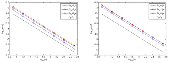
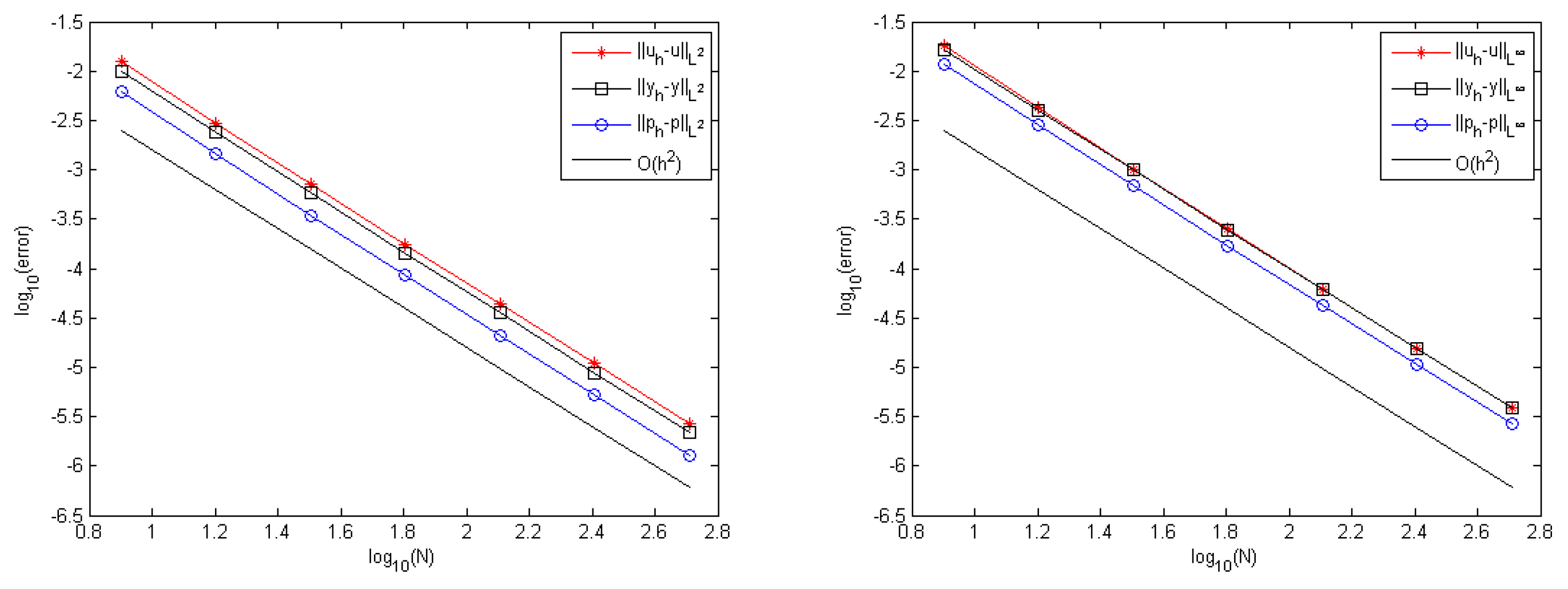
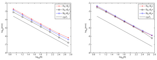
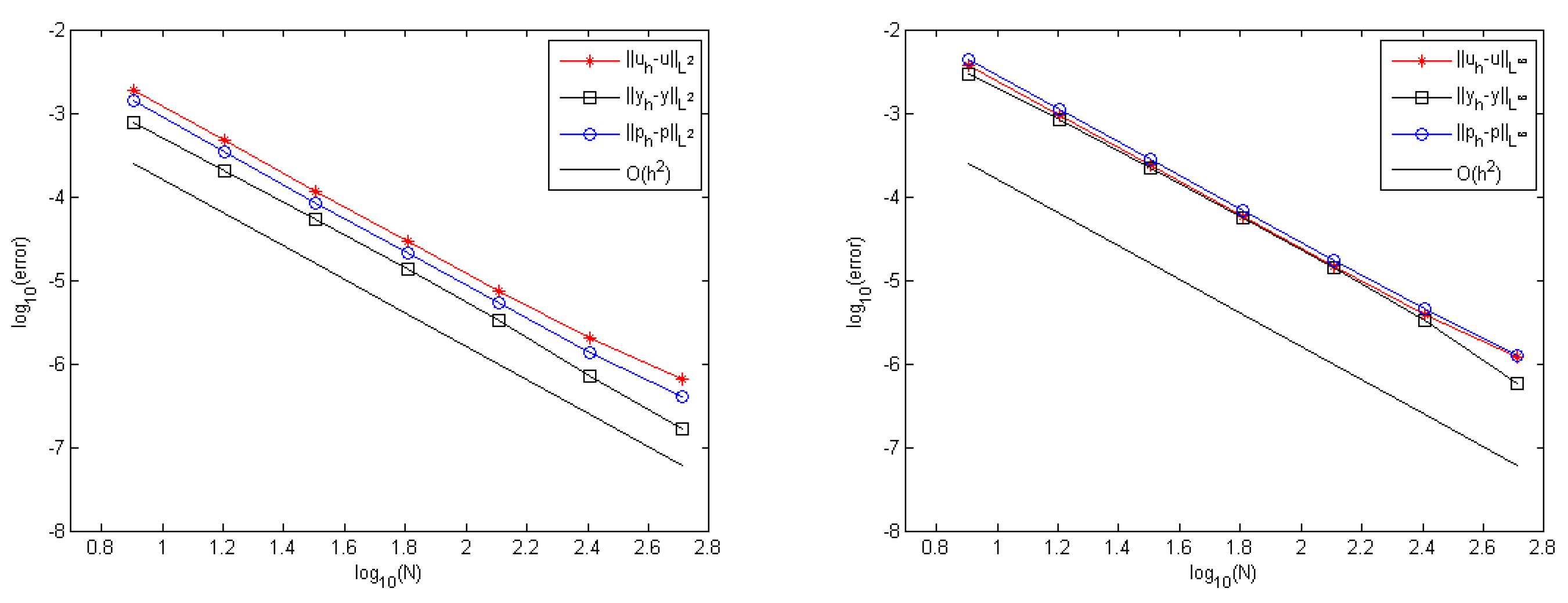
The corresponding numerical results of grid refinement analysis for experiment 1 are presented in Table 1, which contains the error and convergence order of the control u, the state y and the adjoint state p in the sense of both $L^2$-norm and $L^{\infty }$-norm. Figure 2 depicts the convergence orders by slopes. It is apparent that the second order convergence rates of $u,y,p$ are achieved with this methods.

Table 1. Error of control u, state y, and adjoint state p for experiment 1 with fixed L.

(a) $L^2$-norm
N	$\left|\right|u_{f_h}-u{\left|\right|}_{L^2\left(\partial {\Omega }_1\right)}$	Order	$\left|\right|y_{f_h}-y{\left|\right|}_{L^2\left(\Omega \right)}$	Order	$\left|\right|p_{f_h}-p{\left|\right|}_{L^2\left(\Omega \right)}$	Order
8	$1.2641\times {10}^{-2}$		$1.0022\times {10}^{-2}$		$6.1839\times {10}^{-3}$
16	$2.9821\times {10}^{-3}$	2.12	$2.3802\times {10}^{-3}$	2.11	$1.4400\times {10}^{-3}$	2.15
32	$7.2104\times {10}^{-4}$	2.07	$5.7755\times {10}^{-4}$	2.06	$3.4628\times {10}^{-4}$	2.08
64	$1.7706\times {10}^{-4}$	2.04	$1.4208\times {10}^{-4}$	2.03	$8.4826\times {10}^{-5}$	2.04
128	$4.3852\times {10}^{-5}$	2.02	$3.5227\times {10}^{-5}$	2.02	$2.0988\times {10}^{-5}$	2.02
256	$1.0914\times {10}^{-5}$	2.01	$8.7656\times {10}^{-6}$	2.01	$5.2182\times {10}^{-6}$	2.01
512	$2.7245\times {10}^{-6}$	2.00	$2.1842\times {10}^{-6}$	2.01	$1.3001\times {10}^{-6}$	2.01
(b) $L^{\infty }$-norm
N	$\left|\right|u_{f_h}-u{\left|\right|}_{L^{\infty }\left(\partial {\Omega }_1\right)}$	Order	$\left|\right|y_{f_h}-y{\left|\right|}_{L^{\infty }\left(\Omega \right)}$	Order	$\left|\right|p_{f_h}-p{\left|\right|}_{L^{\infty }\left(\Omega \right)}$	Order
8	$1.7877\times {10}^{-2}$		$1.6492\times {10}^{-2}$		$1.1750\times {10}^{-2}$
16	$4.2173\times {10}^{-3}$	2.12	$4.0400\times {10}^{-3}$	2.04	$2.8245\times {10}^{-3}$	2.08
32	$1.0197\times {10}^{-3}$	2.07	$9.9734\times {10}^{-4}$	2.03	$6.9079\times {10}^{-4}$	2.04
64	$2.5040\times {10}^{-4}$	2.04	$2.4758\times {10}^{-4}$	2.01	$1.7070\times {10}^{-4}$	2.02
128	$6.2016\times {10}^{-5}$	2.02	$6.1673\times {10}^{-5}$	2.01	$4.2423\times {10}^{-5}$	2.01
256	$1.5435\times {10}^{-5}$	2.01	$1.5383\times {10}^{-5}$	2.00	$1.0571\times {10}^{-5}$	2.01
512	$3.8531\times {10}^{-6}$	2.00	$3.8379\times {10}^{-6}$	2.00	$2.6369\times {10}^{-6}$	2.00

Figure 2. Convergence orders of $u_{f_h}$ − u, $y_{f_h}$ − y, and $p_{f_h}$ − p in different norms.

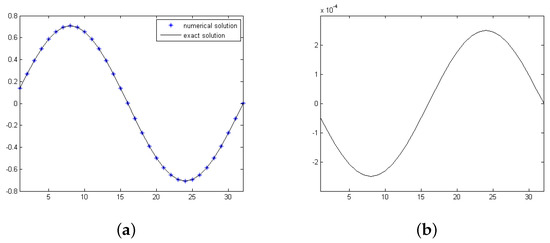
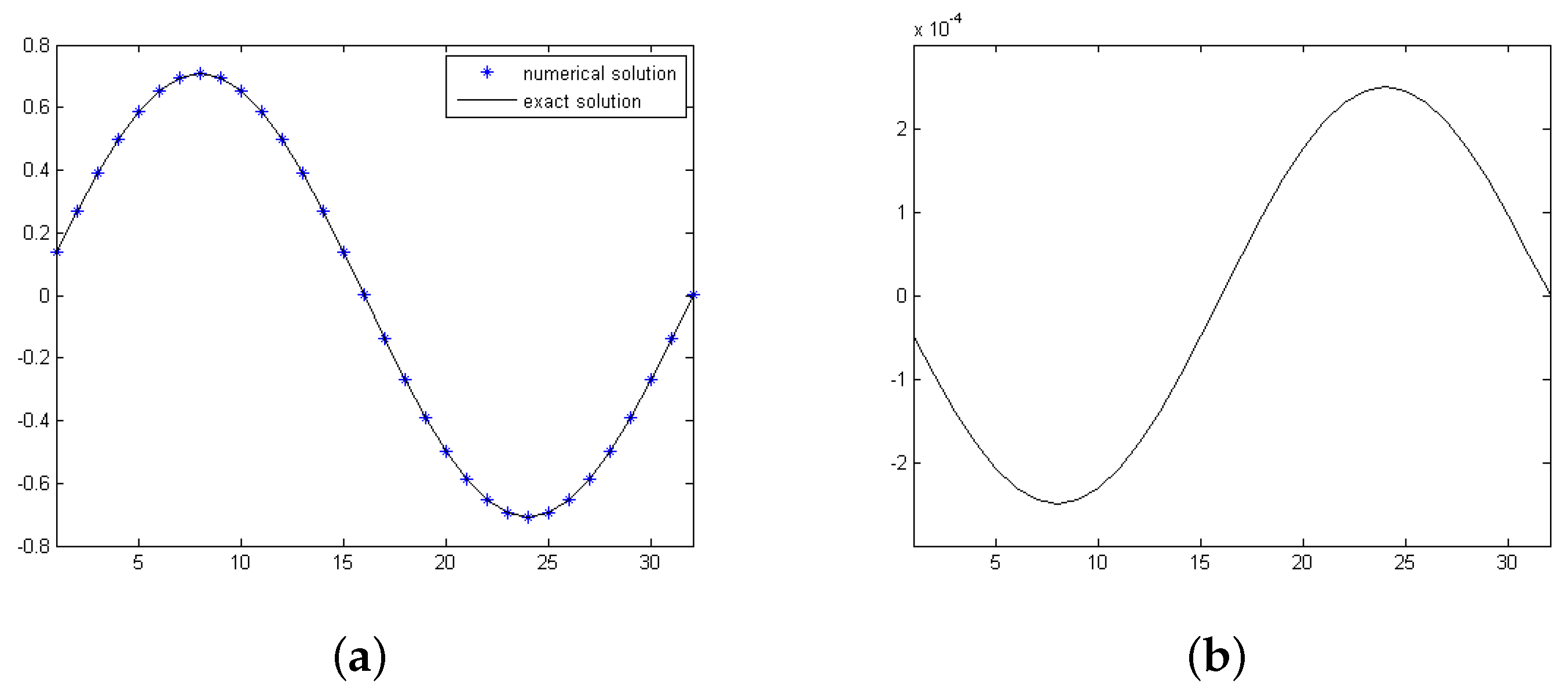
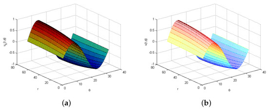
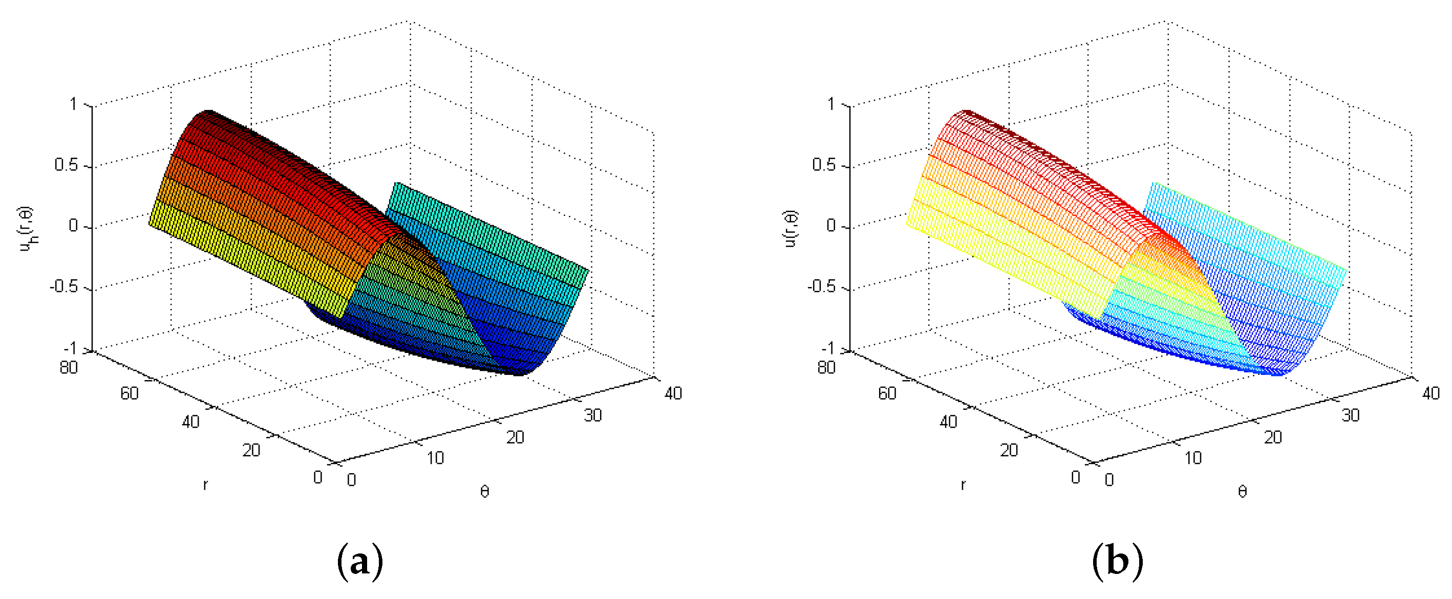
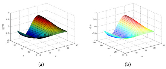
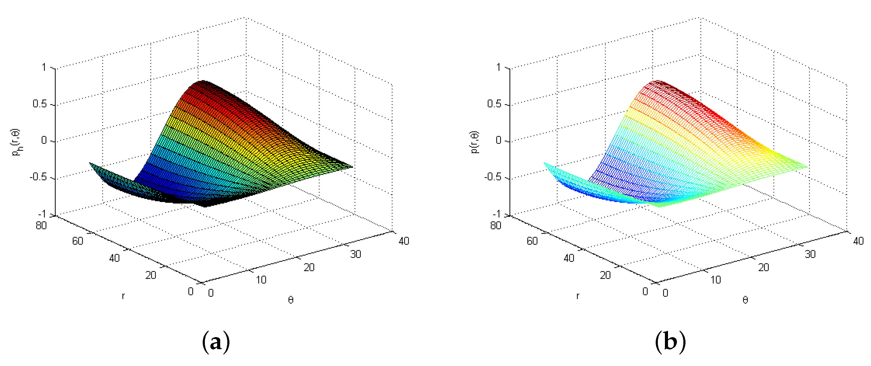
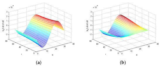
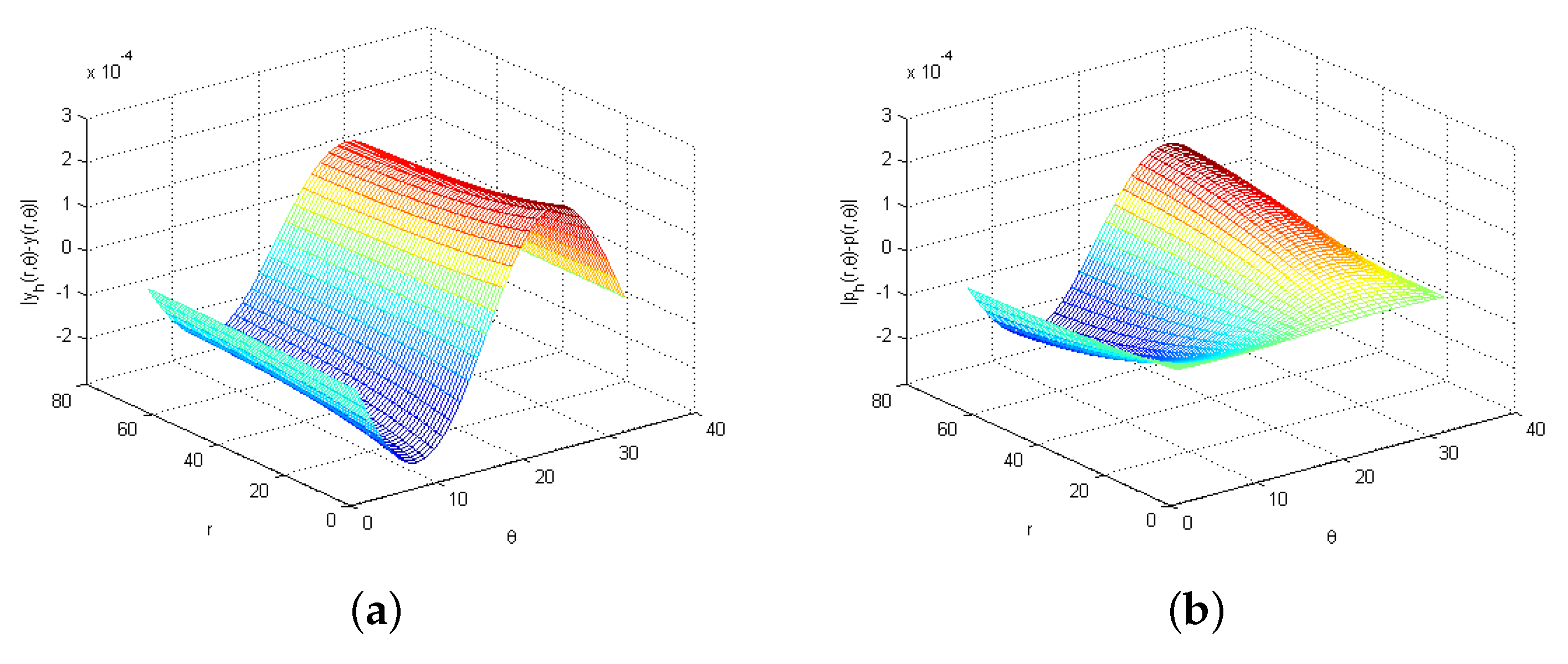
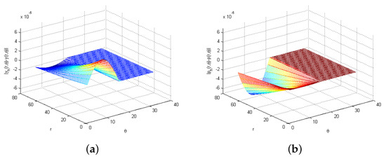
The numerical solution $u_{f_h}$ versus exact solution u with $N=64$ is shown in Figure 3a, and the error of control u is plotted in Figure 3b. Figure 4, Figure 5 and Figure 6 show the numerical solution and the exact solution for the state and adjoint the error between them, respectively. From Figure 6, we find that both errors are of the scale of ${10}^{-4}$ at $N=64$, which indicates that the numerical method has a good approximation.

Figure 3. The numerical solution $u_{f_h}$ versus exact solution u (a), error $u_{f_h}$ − u (b) for experiment 1 with $N=64$.

Figure 4. Numerical solution $y_{f_h}$ (a) and exact solution y (b) with $N=64$.

Figure 5. Numerical solution $p_{f_h}$ (a) and exact solution p (b) with $N=64$.

Figure 6. Error for state y (a) and adjoint state p (b) with $N=64$.

5.2. Experiment 2

The second experiment is an constrained control problem defined on the $\Omega =\{1<x_1^2+x_2^2<2\}$ with

$$\begin{array}{cc}\hfill & f=\frac{1}{\alpha }\left(\frac{5}{r^2}-3\right)max\left(0,sin\theta \right),\hfill \\ \hfill & y_d=\left(\frac{1}{\alpha }{r}^2-\frac{4}{\alpha }r-\frac{3}{r^2}+\frac{5}{\alpha }+3\right)max\left(0,sin\theta \right),\hfill \end{array}$$

the optimal solution is given by

$$\begin{array}{cc}\hfill & y=\frac{1}{\alpha }\left(r^2-4r+5\right)max\left(0,sin\theta \right),\hfill \\ \hfill & p=\left(r^2-4r+3\right)max\left(0,sin\theta \right),\hfill \\ \hfill & u=\frac{2}{\alpha }max\left(0,sin\theta \right),\hfill \end{array}$$

where $\alpha =1.3$ is selected.

Table 2 presents the error and convergence order of the control u, the state y, and the adjoint state p in the sense of both $L^2$-norm and $L^{\infty }$-norm, the corresponding profiles of their convergence order are shown in Figure 7. From them, we derive that the convergence order of these three variables are second.

Table 2. Error of control u, state y and adjoint state p for experiment 2 with fixed L.

(a) $L^2$-norm
N	$\left|\right|u_{f_h}-u{\left|\right|}_{L^2\left(\partial {\Omega }_1\right)}$	Order	$\left|\right|y_{f_h}-y{\left|\right|}_{L^2\left(\Omega \right)}$	Order	$\left|\right|p_{f_h}-p{\left|\right|}_{L^2\left(\Omega \right)}$	Order
8	$1.8638\times {10}^{-3}$		$7.5762\times {10}^{-4}$		$1.4328\times {10}^{-3}$
16	$4.6715\times {10}^{-4}$	1.99	$2.0419\times {10}^{-4}$	1.86	$3.4342\times {10}^{-4}$	2.09
32	$1.1707\times {10}^{-4}$	2.00	$5.2882\times {10}^{-5}$	1.93	$8.4040\times {10}^{-5}$	2.04
64	$2.9414\times {10}^{-5}$	1.99	$1.3358\times {10}^{-5}$	1.98	$2.0831\times {10}^{-5}$	2.02
128	$7.5096\times {10}^{-6}$	1.96	$3.2515\times {10}^{-6}$	2.05	$5.2401\times {10}^{-6}$	1.99
256	$2.0341\times {10}^{-6}$	1.85	$7.1071\times {10}^{-7}$	2.29	$1.3680\times {10}^{-6}$	1.92
(b) $L^{\infty }$-norm
N	$\left|\right|u_{f_h}-u{\left|\right|}_{L^{\infty }\left(\partial {\Omega }_1\right)}$	Order	$\left|\right|y_{f_h}-y{\left|\right|}_{L^{\infty }\left(\Omega \right)}$	Order	$\left|\right|p_{f_h}-p{\left|\right|}_{L^{\infty }\left(\Omega \right)}$	Order
8	$3.7278\times {10}^{-3}$		$2.9252\times {10}^{-3}$		$4.4435\times {10}^{-3}$
16	$9.3417\times {10}^{-4}$	2.00	$8.2853\times {10}^{-4}$	1.77	$1.1098\times {10}^{-3}$	2.00
32	$2.3401\times {10}^{-4}$	2.00	$2.2003\times {10}^{-4}$	1.88	$2.7740\times {10}^{-4}$	2.00
64	$5.8703\times {10}^{-5}$	1.99	$5.6482\times {10}^{-5}$	1.95	$6.9430\times {10}^{-5}$	2.00
128	$1.4881\times {10}^{-5}$	1.97	$1.4089\times {10}^{-5}$	2.00	$1.7464\times {10}^{-5}$	1.99
256	$3.9240\times {10}^{-6}$	1.90	$3.3027\times {10}^{-6}$	2.13	$4.4741\times {10}^{-6}$	1.95

Figure 7. Convergence orders of $u_{f_h}$ − u, $y_{f_h}$ − y, and $p_{f_h}$ − p in different norms.

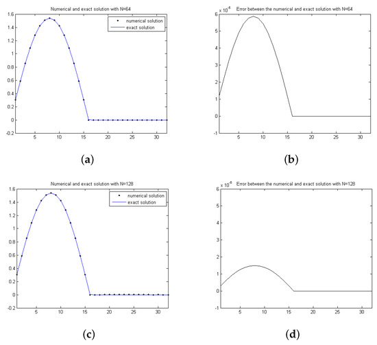
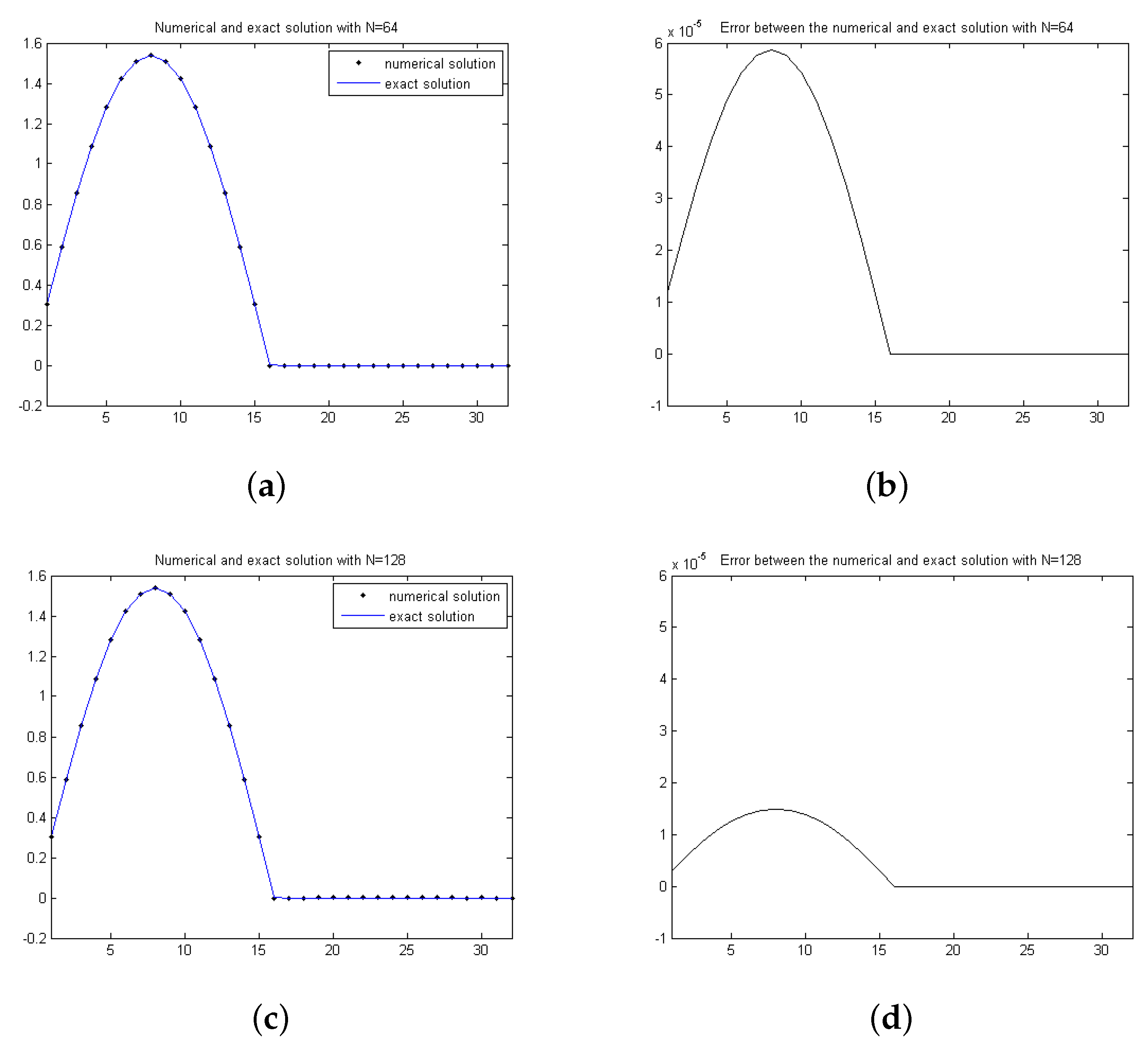
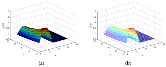
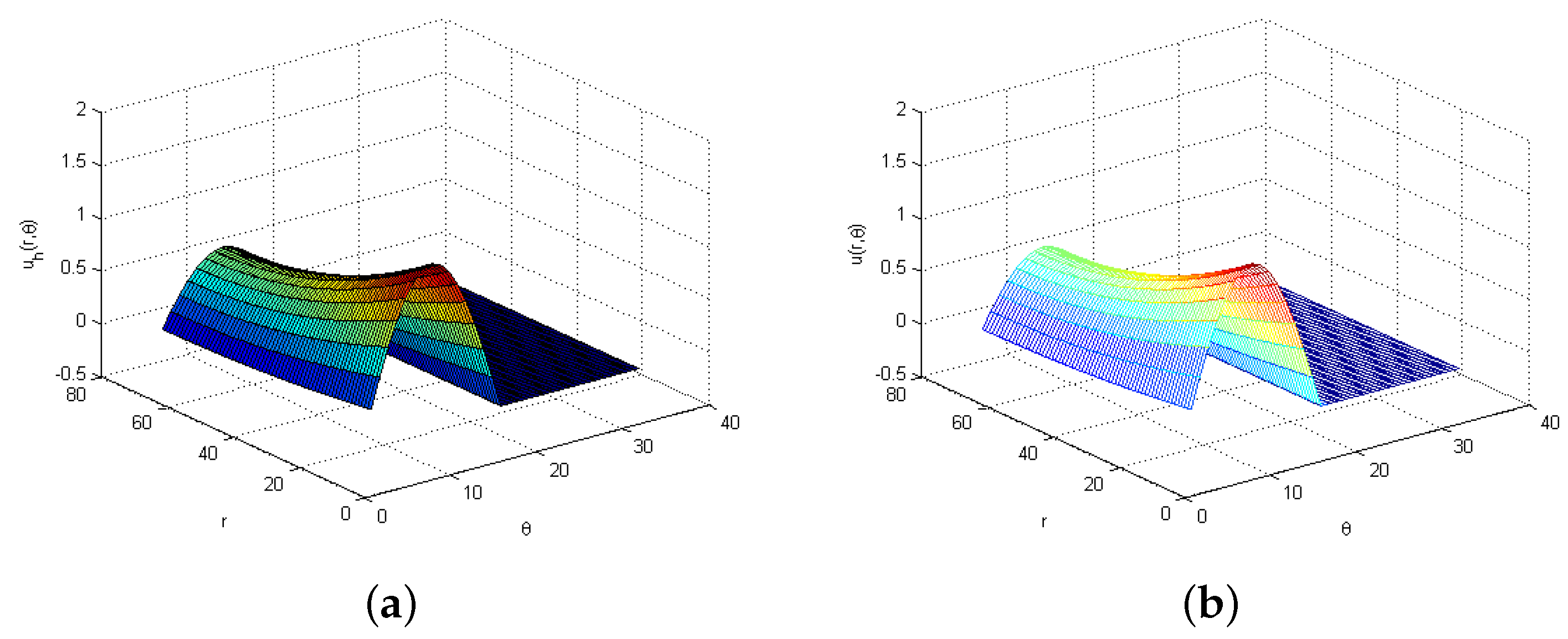
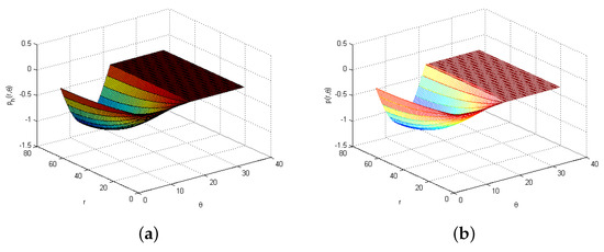
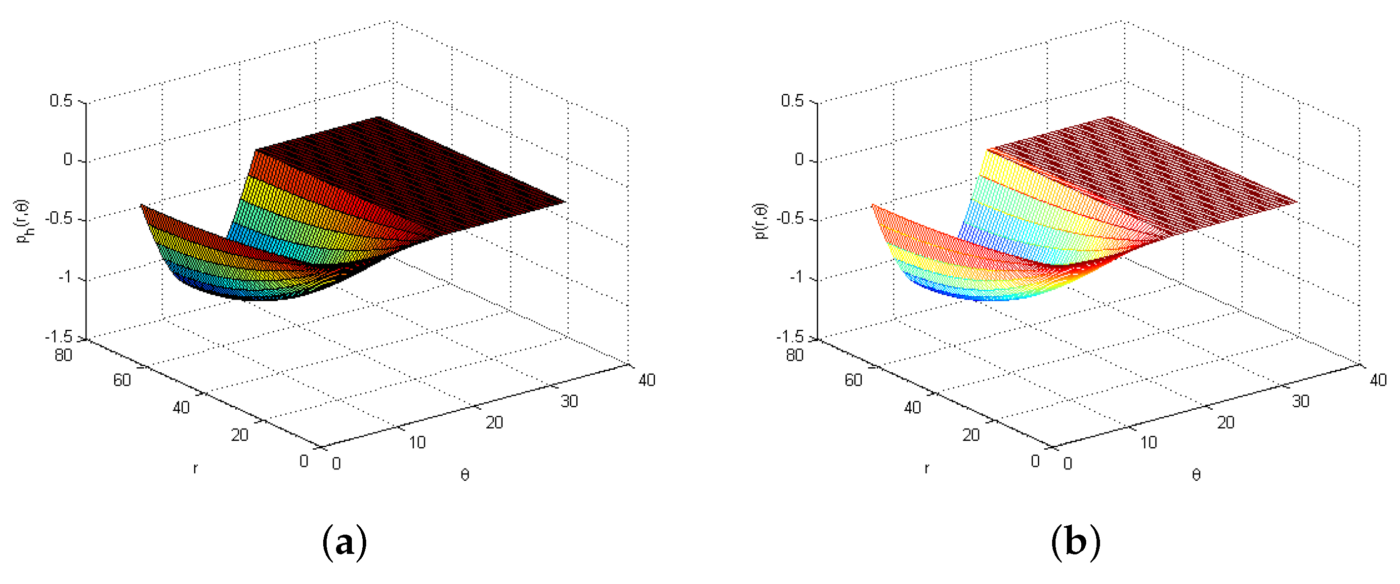
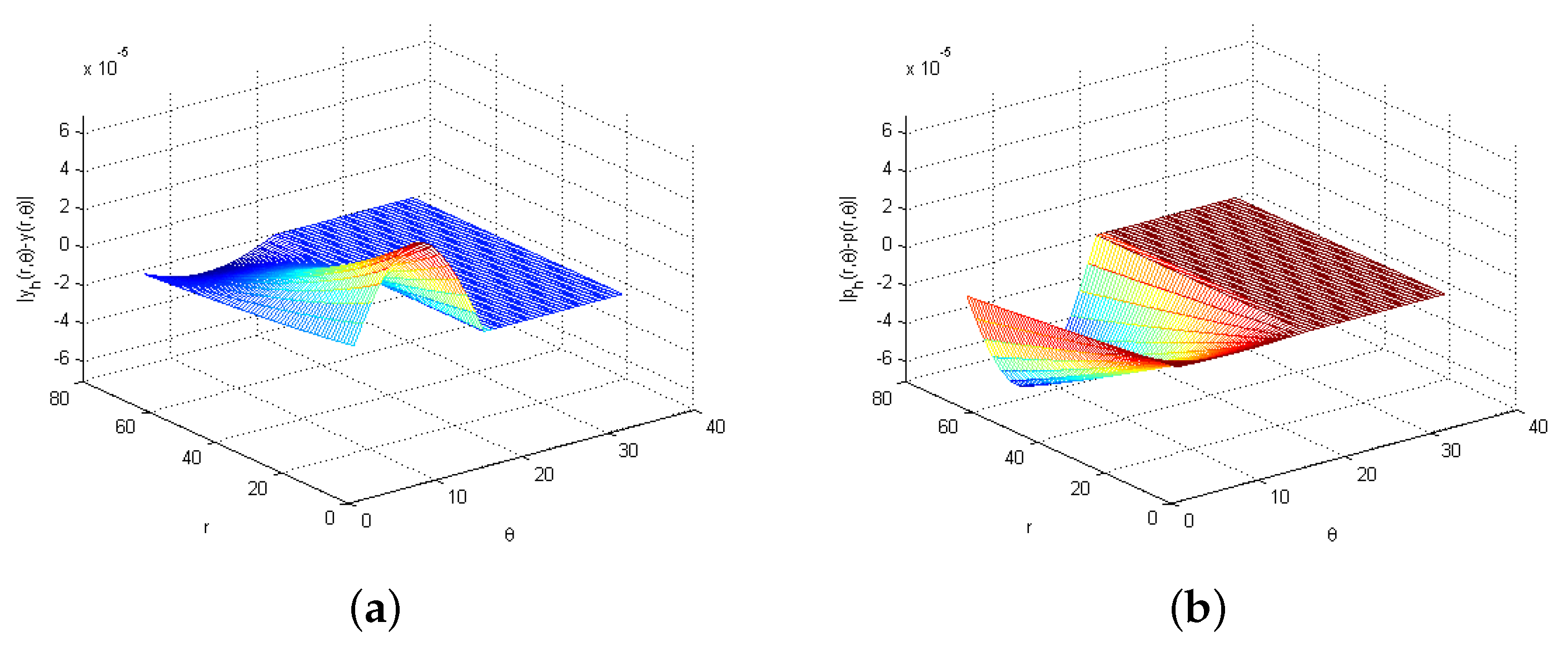
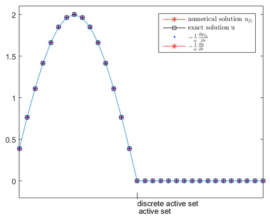
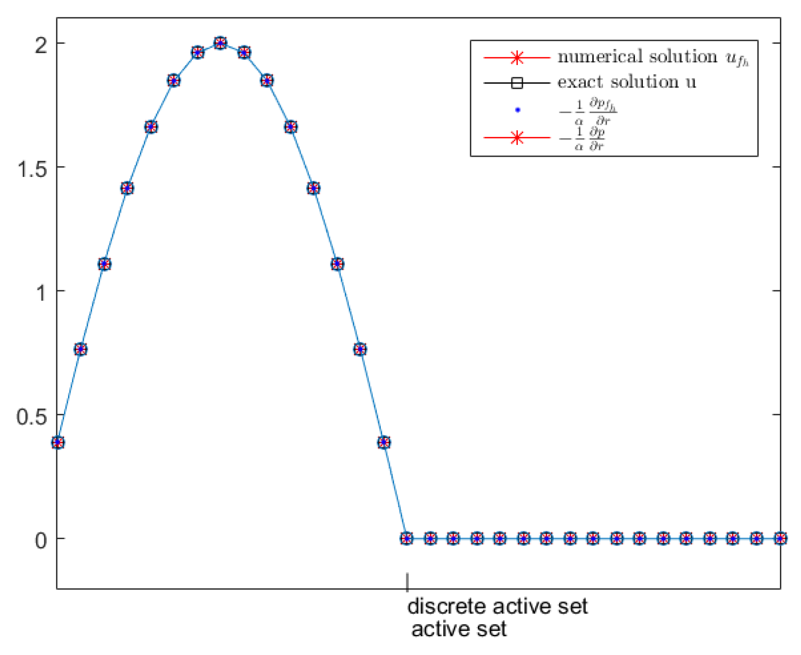
Figure 8a,c describe the profile of the exact and numerical solution of control u, while Figure 8b,d display its numerical error with $N=64$ and $N=128$, respectively. From this figure, we can also observe that the convergence order is second. The numerical solution and the exact solution of the state and adjoint are presented in Figure 9, Figure 10 and Figure 11 and error between them is showed in Figure 11. Figure 12 depicts the continuous Dirichlet boundary control u and discrete Dirichlet boundary control $u_{f_h}$ together with their active sets, it is clear to see that the discrete active set is approximate to active set. These numerical results demonstrate the efficiency of our proposed method.

Figure 8. The numerical solution $u_{f_h}$ versus exact solution u (a,c), error $u_{f_h}$ − u (b,d) for experiment 2.

Figure 9. Numerical solution $y_{f_h}$ (a) and exact solution y (b) with $N=64$.

Figure 10. Numerical solution $p_{f_h}$ (a) and exact solution p (b) with $N=64$.

Figure 11. Error for state y (a) and adjoint state p (b) with $N=64$.

Figure 12. Discrete active set and active set of Dirichlet boundary control u.

6. Concluding Remarks

This research explored an optimal control problem on a complex connected domain governed by elliptic PDEs with Dirichlet boundary conditions. First, the optimality system for the optimal control problem is determined. Then, using the Fourier finite volume element approach to convert this problem into polar coordinates and discretize the optimal control problem. Next, the convergence order of the Dirichlet boundary control, the state, and the adjoint state are proven. This error estimate contains two components: The Fourier truncation error and the one-dimensional finite volume element error. Finally, numerical experiments are shown to back up the theoretical findings.

References

- Han, Q.; Lin, F. Elliptic Partial Differential Equations; American Mathematical Soc.: Providence, RI, USA, 2011; Volume 1. [Google Scholar]
- Nirenberg, L. On elliptic partial differential equations. In Il Principio di Minimo e sue Applicazioni alle Equazioni Funzionali; Springer: Berlin/Heidelberg, Germany, 2011; pp. 1–48. [Google Scholar]
- Boureghda, A. Solution of an ice melting problem using a fixed domain method with a moving boundary. Bull. Math. Soc. Sci. Math. Roum. 2019, 62, 341–353. [Google Scholar]
- Gefen, A.; Weihs, D. Computer Methods in Biomechanics and Biomedical Engineering: Proceedings of the 14th International Symposium CMBBE, Tel Aviv, Israel, 2016; Springer: Cham, Switzerland, 2018. [Google Scholar] [CrossRef] [Scilit]
- Tröltzsch, F. Optimal Control of Partial Differential Equations: Theory, Methods, and Applications; American Mathematical Soc.: Providence, RI, USA, 2010; Volume 112. [Google Scholar]
- Lions, J.L. Optimal Control of Systems Governed by Partial Differential Equations; Springer: Berlin/Heidelberg, Germany, 1971. [Google Scholar]
- Hinze, M.; Pinnau, R.; Ulbrich, M.; Ulbrich, S. Optimization with PDE Constraints; Springer: Berlin/Heidelberg, Germany, 2008; Volume 23. [Google Scholar]
- Zamani, N.; Chuang, J. Optimal control of current in a cathodic protection system: A numerical investigation. Optim. Control Appl. Methods 1987, 8, 339–350. [Google Scholar] [CrossRef] [Scilit]
- Zhong, W.; Zhong, X. Elliptic partial differential equation and optimal control. Numer. Methods Partial Differ. Equ. 1992, 8, 149–169. [Google Scholar]
- Yousept, I. Optimal control of quasilinear H(curl)-elliptic partial differential equations in magnetostatic field problems. SIAM J. Control Optim. 2013, 51, 3624–3651. [Google Scholar] [CrossRef] [Scilit]
- Khursheed, A. The Finite Element Method in Charged Particle Optics; Springer: Boston, MA, USA, 1999. [Google Scholar]
- French, D.A.; Thomas King, J. Approximation of an elliptic control problem by the finite element method. Numer. Funct. Anal. Optim. 1991, 12, 299–314. [Google Scholar] [CrossRef] [Scilit]
- Yan, M.; Gong, W.; Yan, N. Finite element methods for elliptic optimal control problems with boundary observations. Appl. Numer. Math. 2015, 90, 190–207. [Google Scholar] [CrossRef] [Scilit]
- Christof, C.; Vexler, B. New regularity results and finite element error estimates for a class of parabolic optimal control problems with pointwise state constraints. ESAIM Control Optim. Calc. Var. 2021, 27, 4. [Google Scholar] [CrossRef] [Scilit]
- Liu, J.; Zhou, Z. Finite element approximation of time fractional optimal control problem with integral state constraint. AIMS Math. 2021, 6, 979–997. [Google Scholar] [CrossRef] [Scilit]
- Li, R.; Chen, Z.; Wu, W. Generalized Difference Methods for Differential Equations: Numerical Analysis of Finite Volume Methods; CRC Press: New York, NY, USA, 2000. [Google Scholar]
- Shen, J.; Tang, T.; Wang, L. Spectral Methods: Algorithms, Analysis and Applications; Springer: Berlin/Heidelberg, Germany, 2011; Volume 41. [Google Scholar]
- Pfeiffer, H.P.; Kidder, L.E.; Scheel, M.A.; Teukolsky, S.A. A multidomain spectral method for solving elliptic equations. Comput. Phys. Commun. 2003, 152, 253–273. [Google Scholar] [CrossRef] [Scilit]
- Tao, Z.Z.; Sun, B. Galerkin spectral method for elliptic optimal control problem with L2-norm control constraint. Discret. Contin. Dyn. Syst.-B 2022, 27, 4121. [Google Scholar] [CrossRef] [Scilit]
- Chen, R. On optimal boundary control of a class of system governed by parabolic partial differential equation. Sci. China Ser. A-Math. Phys. Astron. Technol. Sci. 1982, 25, 1205–1218. [Google Scholar]
- Casas, E.; Raymond, J.P. Error estimates for the numerical approximation of Dirichlet boundary control for semilinear elliptic equations. SIAM J. Control Optim. 2006, 45, 1586–1611. [Google Scholar] [CrossRef] [Scilit]
- Deckelnick, K.; Günther, A.; Hinze, M. Finite element approximation of Dirichlet boundary control for elliptic PDEs on two-and three-dimensional curved domains. SIAM J. Control Optim. 2009, 48, 2798–2819. [Google Scholar] [CrossRef] [Scilit]
- Gong, W.; Yan, N. Mixed finite element method for Dirichlet boundary control problem governed by elliptic PDEs. SIAM J. Control Optim. 2011, 49, 984–1014. [Google Scholar] [CrossRef] [Scilit]
- Pfefferer, J.; Winkler, M. Finite element error estimates for normal derivatives on boundary concentrated meshes. SIAM J. Control Optim. 2019, 57, 2043–2073. [Google Scholar] [CrossRef] [Scilit]
- Vexler, B. Finite element approximation of elliptic Dirichlet optimal control problems. Numer. Funct. Anal. Optim. 2007, 28, 957–973. [Google Scholar] [CrossRef] [Scilit]
- May, S.; Rannacher, R.; Vexler, B. Error analysis for a finite element approximation of elliptic Dirichlet boundary control problems. SIAM J. Control Optim. 2013, 51, 2585–2611. [Google Scholar] [CrossRef] [Scilit]
- Chang, L.; Gong, W.; Yan, N. Weak boundary penalization for Dirichlet boundary control problems governed by elliptic equations. J. Math. Anal. Appl. 2017, 453, 529–557. [Google Scholar] [CrossRef] [Scilit]
- Hu, W.; Shen, J.; Singler, J.R.; Zhang, Y.; Zheng, X. A superconvergent hybridizable discontinuous Galerkin method for Dirichlet boundary control of elliptic PDEs. Numer. Math. 2020, 144, 375–411. [Google Scholar] [CrossRef] [Scilit]
- Geveci, T. On the approximation of the solution of an optimal control problem governed by an elliptic equation. RAIRO. Anal. Numérique 1979, 13, 313–328. [Google Scholar] [CrossRef] [Scilit]
- Karkulik, M. A finite element method for elliptic Dirichlet boundary control problems. Comput. Methods Appl. Math. 2020, 20, 827–843. [Google Scholar] [CrossRef] [Scilit]
- Hinze, M.; Matthes, U. A note on variational discretization of elliptic Neumann boundary control. Control Cybern. 2009, 38, 577–591. [Google Scholar]
- Casas, E.; Dhamo, V. Error estimates for the numerical approximation of Neumann control problems governed by a class of quasilinear elliptic equations. Comput. Optim. Appl. 2012, 52, 719–756. [Google Scholar] [CrossRef] [Scilit]
- Gunzburger, M.D.; Lee, H.C.; Lee, J. Error estimates of stochastic optimal Neumann boundary control problems. SIAM J. Numer. Anal. 2011, 49, 1532–1552. [Google Scholar] [CrossRef] [Scilit]
- Krumbiegel, K.; Meyer, C.; Rösch, A. A priori error analysis for linear quadratic elliptic Neumann boundary control problems with control and state constraints. SIAM J. Control Optim. 2010, 48, 5108–5142. [Google Scholar] [CrossRef] [Scilit]
- Brenner, S.; Oh, M.; Sung, L.Y. P1 finite element methods for an elliptic state-constrained distributed optimal control problem with Neumann boundary conditions. Results Appl. Math. 2020, 8, 100090. [Google Scholar] [CrossRef] [Scilit]
- Akman, T.; Yücel, H.; Karasözen, B. A priori error analysis of the upwind symmetric interior penalty Galerkin (SIPG) method for the optimal control problems governed by unsteady convection diffusion equations. Comput. Optim. Appl. 2014, 57, 703–729. [Google Scholar] [CrossRef] [Scilit]
- Luo, X.; Chen, Y.; Huang, Y.; Hou, T. Some error estimates of finite volume element method for parabolic optimal control problems. Optim. Control Appl. Methods 2014, 35, 145–165. [Google Scholar] [CrossRef] [Scilit]
- Chen, Y.; Yi, N.; Liu, W. A Legendre–Galerkin spectral method for optimal control problems governed by elliptic equations. SIAM J. Numer. Anal. 2008, 46, 2254–2275. [Google Scholar] [CrossRef] [Scilit]
- Ravindran, S.S. Penalization of Dirichlet Boundary Control for Nonstationary Magneto-Hydrodynamics. SIAM J. Control Optim. 2020, 58, 2354–2382. [Google Scholar] [CrossRef] [Scilit]
- Chatzipantelidis, P.; Lazarov, R.; Thomée, V. Error estimates for a finite volume element method for parabolic equations in convex polygonal domains. Numer. Methods Partial. Differ. Equ. Int. J. 2004, 20, 650–674. [Google Scholar] [CrossRef] [Scilit]
- Bi, C.; Ginting, V. Two-grid finite volume element method for linear and nonlinear elliptic problems. Numer. Math. 2007, 108, 177–198. [Google Scholar] [CrossRef] [Scilit]
- Kumar, S.; Nataraj, N.; Pani, A.K. Finite volume element method for second order hyperbolic equations. Int. J. Numer. Anal. Model. 2008, 5, 132–151. [Google Scholar]
- Luo, X.; Chen, Y.; Huang, Y. Some Error Estimates of Finite Volume Element Approximation for Elliptic Optimal Control Problems. Int. J. Numer. Anal. Model. 2013, 10, 697–711. [Google Scholar]
- Cai, Z.; McCormick, S. On the accuracy of the finite volume element method for diffusion equations on composite grids. SIAM J. Numer. Anal. 1990, 27, 636–655. [Google Scholar] [CrossRef] [Scilit]
- Ewing, R.; Lazarov, R.; Lin, Y. Finite volume element approximations of nonlocal reactive flows in porous media. Numer. Methods Partial. Differ. Equ. Int. J. 2000, 16, 285–311. [Google Scholar] [CrossRef] [Scilit]
- Karaa, S.; Mustapha, K.; Pani, A.K. Finite volume element method for two-dimensional fractional subdiffusion problems. IMA J. Numer. Anal. 2017, 37, 945–964. [Google Scholar] [CrossRef] [Scilit]
- Li, R.; Gao, Y.; Chen, J.; Zhang, L.; He, X.; Chen, Z. Discontinuous finite volume element method for a coupled Navier-Stokes-Cahn-Hilliard phase field model. Adv. Comput. Math. 2020, 46, 1–35. [Google Scholar] [CrossRef] [Scilit]
- Lin, Y.; Liu, J.; Yang, M. Finite volume element methods: An overview on recent developments. Int. J. Numer. Anal. Model. Ser. B 2013, 4, 14–34. [Google Scholar]
- Gan, X.; Xu, D. An efficient symmetric finite volume element method for second-order variable coefficient parabolic integro-differential equations. Comput. Appl. Math. 2020, 39, 1–24. [Google Scholar] [CrossRef] [Scilit]
- Lou, Y.; Chen, C.; Xue, G. Two-grid finite volume element method combined with Crank-Nicolson scheme for semilinear parabolic equations. Adv. Appl. Math. Mech. 2021, 13, 892–913. [Google Scholar]
- Ewing, R.E.; Li, Z.; Lin, T.; Lin, Y. The immersed finite volume element methods for the elliptic interface problems. Math. Comput. Simul. 1999, 50, 63–76. [Google Scholar] [CrossRef] [Scilit]
- Kumar, S.; Nataraj, N.; Pani, A.K. Discontinuous Galerkin finite volume element methods for second-order linear elliptic problems. Numer. Methods Partial. Differ. Equ. Int. J. 2009, 25, 1402–1424. [Google Scholar] [CrossRef] [Scilit]
- Wang, Q.; Zhang, Z.; Li, Z. A Fourier finite volume element method for solving two-dimensional quasi-geostrophic equations on a sphere. Appl. Numer. Math. 2013, 71, 1–13. [Google Scholar]
- Lin, X.; Su, M.; Zhang, Z. Fourier Finite Volume Element Method for Two Classes of Optimal Control Problems Governed by Elliptic PDEs on Complex Connected Domain. Numer. Funct. Anal. Optim. 2020, 41, 379–412. [Google Scholar] [CrossRef] [Scilit]
- Hinze, M. A variational discretization concept in control constrained optimization: The linear-quadratic case. Comput. Optim. Appl. 2005, 30, 45–61. [Google Scholar] [CrossRef] [Scilit]
- Chen, R. Optimal boundary control of parabolic system on doubly connected region in new space. Sci. China (Sci. Sin.) Ser. A 1995, 8, 933–944. [Google Scholar]
- Djellab, N. Résolution Numérique de Problèmes D’équations aux Dérivées Partielles Issus de la Biologie et la Médecine. Ph.D. Thesis, Ferhat ABBAS University, Setif, Algeria, 2022. [Google Scholar]
- Ewing, R.E.; Lin, T.; Lin, Y. On the accuracy of the finite volume element method based on piecewise linear polynomials. SIAM J. Numer. Anal. 2002, 39, 1865–1888. [Google Scholar] [CrossRef] [Scilit]
- Qiu, Z.; Zeng, Z.; Mei, H.; Li, L.; Yao, L.; Zhang, L. A Fourier–Legendre spectral element method in polar coordinates. J. Comput. Phys. 2012, 231, 666–675. [Google Scholar] [CrossRef] [Scilit]
Publisher’s Note: MDPI stays neutral with regard to jurisdictional claims in published maps and institutional affiliations. |
© 2022 by the authors. Licensee MDPI, Basel, Switzerland. This article is an open access article distributed under the terms and conditions of the Creative Commons Attribution (CC BY) license (https://creativecommons.org/licenses/by/4.0/).