


Abstract
This paper conducts a comprehensive empirical evaluation of macroeconomic outcomes under two competing policy paradigms that have governed the United States since the end of World War II: the Keynesian-inflected New Deal Order (1946–1980), rooted in John Maynard Keynes’s theory of aggregate demand management, and the Neoliberal Order (1981–2024), shaped by the price mechanism epistemics of Friedrich A. Hayek and the monetarist counter-revolution of Milton Friedman. Drawing on the historiographical frameworks we operationalize the 1981 policy transition as a natural experiment and apply a fourteen-component analytical pipeline to an annual panel of fifteen Federal Reserve Economic Data (FRED) series spanning 1946–2024. Our methods include: Pruned Exact Linear Time (PELT) structural break detection; normality-adaptive hypothesis testing with Cohen’s d effect sizes; Principal Component Analysis (PCA); a gradient-boosted XGBoost classifier with SHAP interpretability; static and rolling Phillips curve estimation; bootstrapped fiscal multiplier analysis using the corrected Federal Surplus/Deficit ratio; Composite Macroeconomic Performance Index (CMPI) construction; Pearson correlation structure comparison; regime-stratified Okun’s Law analysis; real federal fund rate and yield curve decomposition; M2 velocity and monetary transmission analysis; k-means sub-period temporal clustering; and government debt trajectory with decade-level performance benchmarking. The Keynesian era produced significantly higher mean real GDP growth (3.7% vs. 2.7%), lower structural unemployment (5.0% vs. 6.2%), and a functioning Phillips curve trade-off that collapsed entirely under neoliberalism (, ). The real federal fund rate averaged negative under the Keynesian regime and turned persistently positive after the Volcker shock. M2 velocity declined sharply in the neoliberal era, refuting the stable quantity theory link central to monetarist policy prescriptions. Temporal clustering recovers five distinct macroeconomic epochs that only partially align with the 1981 historiographical boundary, revealing substantial heterogeneity within each broad regime. The Reagan-era debt expansion, made visible by the corrected debt/GDP trajectory, constitutes a striking empirical contradiction to neoliberal fiscal rhetoric. Together, these results support the interpretation that the two policy regimes represent genuinely distinct macroeconomic equilibria with persistent and measurable consequences for growth, employment, price stability, monetary transmission, and fiscal sustainability. A battery of robustness checks addressing confounding structural shocks, alternative regime boundaries, policy endogeneity, model complexity, and index-construction sensitivity confirms that the core findings are not artifacts of the 1981 periodization, and a cluster-validity analysis formally supports a five-epoch, rather than strictly binary, characterization of the postwar policy landscape.
Keywords:
Keynesian economics; neoliberalism; Hayek; Keynes; fiscal policy; monetary policy; macroeconomic regimes; machine learning; SHAP; XGBoost; structural break analysis; Okun’s law; Phillips curve; M2 velocity; fiscal multiplier; policy evaluation; FRED; temporal clustering; real policy rate; income inequality; New Deal Order; Great Moderation 1. Introduction
Few questions in economics carry as much normative weight, or as much empirical ambiguity, as whether the macroeconomic policy framework governing a national economy makes a systematic difference to long-run welfare and growth. Since the end of World War II, the United States has been governed under two broad and ideologically antithetical policy paradigms. From 1946 to approximately 1980, the macroeconomy was steered by a Keynesian consensus codified in the Employment Act of 1946: discretionary fiscal intervention, active demand management, and a state-guaranteed commitment to maximum employment (Keynes, 1936; Wapshott, 2011). Beginning in 1981, inaugurated by the Reagan administration while the Volcker disinflation was already underway, a neoliberal order supplanted the Keynesian consensus, prioritizing monetary discipline over fiscal activism, supply-side tax reform, deregulation, and a reduction in state intervention in economic life justified by Hayek’s price mechanism epistemology and Friedman’s monetarism (Friedman & Schwartz, 1963; Gerstle, 2022; Harvey, 2005; Hayek, 1944, 1945, 1960).
The intellectual genealogy of this transition is rigorously traced by Wapshott (2011), whose account of the Keynes–Hayek intellectual confrontation of the 1930s frames the entire postwar macroeconomic settlement as an unresolved contest between two incompatible theories of economic order: Keynes’s view that aggregate demand deficiencies produce involuntary unemployment that markets cannot self-correct (Keynes, 1936), and Hayek’s view that the price mechanism aggregates dispersed knowledge no central authority can possess, rendering activist intervention both epistemically futile and structurally damaging (Hayek, 1945). Gerstle (2022) provides the complementary political economy account, showing how the New Deal Order, forged in the Depression and sustained through the Cold War, was dismantled across three decades through the intellectual infrastructure of the Mont Pèlerin Society (Wapshott, 2011), the Heritage Foundation, and the Reagan-era coalition of supply-siders, evangelical social conservatives, and neoliberal technocrats.
What has remained comparatively underexplored is a systematic, multi-dimensional empirical comparison of the macroeconomic outcomes generated under these two regimes across the full 80-year postwar horizon. Most existing assessments rely on single-indicator comparisons, stylized narratives, or short event windows. This paper addresses that gap. Drawing on fifteen macroeconomic time series from the Federal Reserve Economic Data (FRED) repository, we construct an annual panel spanning 1946–2024 and apply a fourteen-component analytical pipeline that combines classical econometrics, machine learning interpretability, and monetary–fiscal diagnostic analysis to evaluate regime-level divergence across growth, employment, inflation, monetary transmission, and fiscal sustainability.
Concretely, the empirical pipeline is organized around four research questions. RQ1: Did the U.S. macroeconomy undergo a fundamental structural change around 1981, or is any apparent shift better explained by gradual trends or by unrelated concurrent shocks? We address RQ1 with the PELT structural break algorithm (Section 3), the confound window exclusion and alternative regime boundary robustness checks (Section 3.4), and the k-means temporal clustering (Section 4.13). RQ2: Did the key structural relationships of macroeconomic theory, the Phillips curve, Okun’s Law, and the money–velocity link, change across the two regimes? We address RQ2 with the regime-stratified and confound-controlled Phillips curve and Okun’s Law regressions (Section 4.10 and Section 3.4) and the M2 velocity analysis (Section 4.12). RQ3: Did policy effectiveness, specifically fiscal multipliers and monetary transmission, change? We address RQ3 with the bootstrapped fiscal multiplier analysis and the real policy rate decomposition. RQ4: Was aggregate economic performance better or worse under one regime than the other, and is that comparison an artifact of a specific choice of policy boundary, indicator weighting, or classification model? We address RQ4 with the CMPI, its weighting scheme robustness checks, and the model complexity comparisons discussed in Section 3.4. The Discussion (Section 6) is organized to answer each of these four questions in turn.
Our contributions are fivefold. First, we operationalize the 1981 political–economic transition as a natural experiment, using the regime boundary both as a treatment variable for supervised learning classification and as a prior for unsupervised structural break detection. Second, we extend the regime comparison beyond the standard GDP/unemployment/inflation triad to include Okun’s Law dynamics, real policy rate regimes, M2 velocity and monetary transmission, sub-period temporal clustering, and government debt trajectory, providing a more complete empirical portrait than any single prior study. Third, we apply SHAP values (Lundberg & Lee, 2017) as an interpretability tool for the macroeconomic regime classification, demonstrating their utility for identifying which indicators carry the most structural discriminating power. Fourth, we correct a systematic data error in the original fiscal impulse analysis, replacing a nominal government expenditure level series (W068RCQ027SBEA) with the Federal Surplus/Deficit as a Percentage of GDP (FYFSGDA188S), and discuss its implications for multiplier estimation and SHAP feature attribution. Fifth, we subject the 1981 periodization itself to a battery of identification checks—exclusion of the 1971–1982 confound window, comparison against alternative historically motivated boundary years, confound-controlled regression models, Granger-causality tests of policy endogeneity, a model complexity benchmark against logistic regression with a label-permutation test, and a multi-scheme robustness test of the CMPI’s index weights—and we formally test, via silhouette and inertia diagnostics, whether a binary regime split or a richer multi-cluster typology is better supported by the data.
Central findings are that the Keynesian era produced higher average real GDP growth, lower structural unemployment, and a functioning Okun’s Law linkage between output growth and employment creation. The neoliberal era delivered sustained disinflation but also a collapse of the Phillips curve, a prolonged decline in M2 velocity that refuted the stable quantity theory link central to monetarist prescriptions, persistently positive real interest rates that penalized debtors and borrowers, and a secular expansion of government debt that belied its own rhetoric of fiscal restraint. These results converge on a nuanced verdict that resists both triumphalist neoliberal narratives and uncritical Keynesian nostalgia, while providing a data-grounded foundation for contemporary policy deliberation.
The remainder of the paper proceeds as follows. Section 2 reviews the relevant theoretical and empirical literature, including a definitional discussion of Keynesianism, neoliberalism, and the “policy regime”/“economic ideology” distinction. Section 3 describes the data and analytical pipeline, including the identification and robustness protocol of Section 3.4. Section 4 presents all empirical results. Section 5 synthesizes cross-cutting observations and methodological caveats. Section 6 situates findings within the broader scholarly debate. Section 7 identifies future research directions, and Section 8 concludes.
2. Literature Review
2.1. Conceptualizing Keynesianism and Neoliberalism: Definitions, Dirigisme, and the “Policy Regime” vs. “Economic Ideology” Distinction
Before reviewing the substantive literature, it is necessary to define the two central constructs of this paper more precisely, since both “Keynesianism” and “neoliberalism” admit multiple, sometimes incompatible, meanings in the scholarly literature. We use Keynesianism to denote the specific policy syndrome, codified in the U.S. Employment Act of 1946 and elaborated through the Hicks–Hansen IS-LM apparatus, in which discretionary fiscal policy and countercyclical demand management are the primary macroeconomic stabilization instruments, wage and price rigidities are treated as structural features rather than frictions to be eliminated, and full employment is an explicit, legislatively mandated policy objective (Keynes, 1936; Wapshott, 2011). This is a narrower construct than dirigisme, the broader tradition of state direction of economic life that Shonfield (1965) documents across postwar Western Europe, encompassing not only demand management but also indicative planning, state ownership of strategic industries, and direct industrial policy. American postwar Keynesianism was, in Shonfield’s (1965) comparative terms, a comparatively mild variant of dirigisme, one confined largely to macroeconomic demand management via fiscal and monetary policy rather than the more extensive industrial planning practiced contemporaneously in France or Japan. We adopt this narrower, demand-management-centered definition of Keynesianism throughout, and flag explicitly where our claims would not extend to the broader dirigiste tradition.
Similarly, we use neoliberalism in the sense developed by Gerstle (2022) and Harvey (2005): a policy syndrome prioritizing monetary discipline over fiscal activism, deregulation of product, labor, and financial markets, and a reduced role for the state in demand management, legitimized by Hayek’s (1944, 1945) epistemic critique of central planning and Friedman’s (1968) monetarism. We emphasize, following Mirowski and Plehwe (2009), Peck (2010), and Boas and Gans-Morse (2009), that this label is analytically convenient but historiographically imprecise: it aggregates at least three distinguishable intellectual and political projects that do not always agree with one another, namely (i) Chicago School monetarism, which retains a rule-based role for the central bank and is largely agnostic about the size of the welfare state provided monetary policy is disciplined (Friedman, 1956, 1968); (ii) Hayekian and Austrian epistemic liberalism, which is skeptical of monetary activism and of the possibility of technocratic fine-tuning more broadly (Hayek, 1944, 1945); and (iii) the supply-side and Mont Pèlerin-network political project documented by Gerstle (2022) and Mirowski and Plehwe (2009), which combined tax-cut advocacy with continued, and in practice expanded, government borrowing. Boas and Gans-Morse (2009) further document that “neoliberalism” functions in much of the empirical political economy literature as a contested, frequently pejorative label applied asymmetrically across cases, a caution we take seriously in restricting our own use of the term to the specific, operationally defined U.S. policy syndrome of 1981–2024 rather than to neoliberalism as a general theoretical category. Section 4.17 operationalizes this distinction empirically, showing that the 1981–2024 period itself decomposes into macroeconomically distinct sub-regimes (Volcker-era monetarist disinflation, Reagan-era supply-side fiscal expansion, Great Moderation inflation-targeting, and post-2008 unconventional monetary policy) that correspond reasonably well to these different intellectual strands, rather than treating “neoliberalism” as a single undifferentiated school throughout.
Finally, we clarify our use of policy regime versus economic ideology. Following Hall’s (1989) account of Keynesianism’s diffusion across nations, we use economic ideology to refer to the underlying normative and theoretical belief system, e.g., the propositions that aggregate demand deficiencies cause involuntary unemployment (a Keynesian ideological commitment) or that decentralized price signals are epistemically superior to central planning (a Hayekian ideological commitment). We reserve policy regime for the empirically observable, data-identifiable configuration of fiscal, monetary, and regulatory settings that a given administration actually implements, which may only imperfectly reflect its stated ideology; Wapshott’s (2011) observation that Reagan’s large deficit-financed tax cuts and defense buildup amounted to “involuntary anonymous Keynesianism” is precisely an instance in which the policy regime (a large, debt-financed demand expansion) diverged from the stated economic ideology (fiscal restraint and supply-side non-intervention). Our empirical analysis is a study of policy regimes as revealed by macroeconomic outcomes data; we do not claim to measure ideological commitment directly, and we flag this distinction wherever the two could be conflated.
2.2. Political Economy of Macroeconomic Regimes
The postwar history of U.S. macroeconomic policy can be understood as a series of contested political–economic orders, stable configurations of institutions, ideas, and coalitions that define the boundaries of legitimate policy action until a crisis shatters them (Gerstle, 2022). Gerstle traces the New Deal Order’s origins in Roosevelt’s response to the Depression: the Glass–Steagall Act (1933) (U.S. Congress, 1933) the Securities and Exchange Commission (1934) (U.S. Congress, 1934), the National Labor Relations Act (1935) (U.S. Congress, 1935), and, critically, the Employment Act of 1946 (U.S. Congress, 1946), which codified the federal government’s responsibility for maintaining “maximum employment, production, and purchasing power” as a constitutional-level commitment. The intellectual scaffolding for this order was supplied by Keynes’s General Theory (Keynes, 1936), which explained unemployment as a demand deficiency that markets could not self-correct, and which was popularized for American policymakers through Samuelson’s seminal textbook (Mankiw et al., 1992) and through the IS-LM formalization of Hicks and Hansen.
Gerstle’s (2022) account of the neoliberal order’s construction proceeds in three acts: Reagan’s political revolution, which targeted the New Deal’s two pillars, collective bargaining and progressive taxation, and reducing the top marginal rate from 70% to 28% while defeating the PATCO air-traffic controllers’ union to signal the state’s withdrawal from labor market support; Clinton’s Democratic acquiescence, manifest in NAFTA, the repeal of Glass–Steagall via the Gramm–Leach–Bliley Act, and the preference for balanced budgets over social investment; and Bush’s “ownership society” hubris, which extended deregulated mortgage markets to low-income households and ultimately precipitated the Global Financial Crisis (Mian & Sufi, 2014). Harvey (2005, 2007) provides a parallel account grounded in political economy, arguing that neoliberalism served as a class project to restore capital accumulation and dismantle the redistributive institutions of the Keynesian settlement, with deregulation and financialization serving as the primary mechanisms.
2.3. Keynesian Theoretical Foundations and the IS-LM Framework
Keynes’s General Theory of Employment, Interest and Money (Keynes, 1936) constituted a fundamental break with classical economics on three dimensions. First, it replaced Say’s Law, that supply creates its own demand, with the principle that aggregate demand is the primary determinant of output and employment in the short run. Second, it introduced the concept of involuntary unemployment: workers can remain unemployed even at prevailing wages because firms lack effective demand for their output, not because wages are too high (Wapshott, 2011). Third, it formalized the multiplier mechanism: each unit of government expenditure generates more than one unit of aggregate output because successive rounds of re-spending amplify the initial injection, a principle originally identified by Kahn and developed by Keynes into the cornerstone of fiscal policy effectiveness. Wapshott (2011) notes that Keynes’s articulation of this principle was direct: “Every job created by the government would add a further job to supply that new worker with goods. The greater trade activity would make for further trade activity; for the forces of prosperity, like those of a trade depression, work with a cumulative effect.”
The IS-LM model, formalized by Hicks and extended by Hansen for American conditions, translated Keynes’s theory into a tractable policy framework that dominated postwar macroeconomics through the 1970s. Samuelson and Solow (1960) operationalized this framework for U.S. anti-inflation policy, identifying the Phillips curve trade-off as the empirical basis for fine-tuning aggregate demand: policymakers could exchange lower unemployment for higher inflation by shifting demand, or vice versa. The Kennedy–Johnson period represented the high-water mark of applied Keynesianism: Kennedy’s tax cuts of 1964, designed explicitly to stimulate demand, reduced unemployment from 4.5% to 3.9% while initially keeping inflation subdued, validating the Phillips curve framework in real time (Wapshott, 2011).
2.4. Hayek’s Price Mechanism and the Epistemics of Intervention
Hayek’s central contribution to the anti-Keynesian critique was not primarily macroeconomic but epistemological. In his landmark 1945 American Economic Review paper (Hayek, 1945), Hayek argued that the relevant economic knowledge—of preferences, local conditions, and specific circumstances of time and place—is irremediably dispersed across millions of individuals and cannot be centralized without catastrophic loss of information. The price system, operating through a decentralized exchange, serves as a “mechanism for communicating information” that aggregates this distributed knowledge into relative price signals, coordinating the decisions of agents who know nothing about each other. This epistemic argument renders activist fiscal and monetary policy not merely inefficient but fundamentally misguided: policymakers cannot possess the knowledge required to improve on the market’s spontaneous coordination.
In The Road to Serfdom (Hayek, 1944) and The Constitution of Liberty (Hayek, 1960), Hayek extended this epistemic argument into a political philosophy: government must operate through general, non-discriminatory rules,“a government of laws, not of men”, rather than through discretionary interventions tailored to specific circumstances. The Austrian Business Cycle Theory, developed by Hayek, building on Mises and Wicksell, held that credit expansion below the natural rate of interest distorts the capital structure by encouraging malinvestment in “roundabout” production processes that cannot be sustained once the artificial stimulus is withdrawn; the subsequent recession is thus not a policy failure but the necessary liquidation of prior distortions (Wapshott, 2011). This framework predicted that Keynesian demand management would produce stagflation, rising prices alongside rising unemployment, when the artificial stimulus encountered supply constraints. The 1970s appeared to vindicate this prediction.
Hayek’s influence grew substantially after he received the Nobel Memorial Prize in Economics in 1974, just as stagflation was discrediting the Keynesian consensus. His ideas filtered into the practical policy agenda of Thatcher and Reagan through the networks of the Mont Pèlerin Society, the Heritage Foundation, and the Manhattan Institute, providing an intellectual legitimization for the political project of state retrenchment that Gerstle (2022) documents in detail. Wapshott (2011) notes, with some irony, that Reagan’s actual fiscal policy, a combination of large tax cuts and rising military spending that produced record peacetime deficits, was “involuntary anonymous Keynesianism” in Robert Solow’s phrase: a deficit-driven demand expansion dressed in Hayekian rhetoric.
2.5. The Monetarist Counter-Revolution and Natural Rate Hypothesis
Friedman’s (1968) presidential address to the American Economic Association delivered the decisive theoretical blow to the Keynesian Phillips curve. By distinguishing the short-run trade-off (exploitable temporarily but not permanently) from the long-run vertical Phillips curve at the natural rate of unemployment, Friedman argued that any attempt to hold unemployment below its natural rate would simply accelerate inflation without reducing unemployment. Phelps (1968) developed an equivalent framework grounded in adaptive expectations. Friedman’s prior work on the quantity theory (Friedman, 1956) and his monetarist rule, that the money supply should grow at a constant rate consistent with stable prices, offered an alternative to Keynesian discretion that appealed to policymakers seeking a rule-based nominal anchor.
The Lucas Critique (Lucas, 1976) extended this challenge: structural relationships estimated under one policy regime are unreliable guides to outcomes under a different one, since rational agents will adjust their behavior to anticipated policy rules. This epistemological challenge is directly relevant to cross-regime comparisons such as ours and motivates the regime-stratified estimation approach adopted throughout this paper. Clarida et al. (2000) estimate that post-Volcker monetary policy implemented a response coefficient to inflation deviations substantially greater than unity, the “Taylor principle”, consistent with a structural shift in the Fed’s preferences toward price stability over output stabilization.
2.6. Structural Change and the Great Moderation
A substantial empirical literature documents a structural break in U.S. macroeconomic volatility in the early 1980s. McConnell and Pérez-Quirós (2000) identify a statistically significant decline in GDP growth volatility around 1984. Kim and Nelson (1999) confirm this using a Bayesian Markov-switching model. Stock and Watson (2002) characterize the Great Moderation as a combination of improved monetary policy, smaller exogenous shocks, and structural changes in inventory management. Gordon (2016) situates this in the longer sweep of American economic history, arguing that the extraordinary growth miracle of 1870–1970 was driven by non-repeatable innovations, electrification, the internal combustion engine, and indoor plumbing, and that the secular deceleration of productivity growth beginning in the 1970s pre-dates the neoliberal transition and reflects the exhaustion of these one-time transformative technologies.
The structural break methodology applied in this paper builds directly on the Bai–Perron framework (Bai & Perron, 1998, 2003) and its nonparametric extension via the PELT algorithm (Killick et al., 2012), which enables detection of distributional shifts rather than merely conditional mean changes.
2.7. Minsky, Financialization, and the Fragility of Stability
Hyman Minsky’s Financial Instability Hypothesis (Minsky, 1986, 1992) provides one of the most prescient frameworks for understanding the GFC and the broader trajectory of the neoliberal financial system. Minsky argued that capitalist economies endogenously generate fragility through periods of stability: as expansion continues, agents reduce their margin of safety and progressively shift from “hedge finance” (revenues cover debt service) to “speculative finance” (revenues cover interest only) and ultimately “Ponzi finance” (revenues cannot cover interest, requiring asset price appreciation for solvency). The prolonged stability of the Great Moderation thus paradoxically increased systemic fragility, as leverage ratios expanded and risk premia compressed to unsustainable levels, the conditions that produced the Minsky Moment of 2007–2008.
Minsky’s framework provides an important corrective to both the Keynesian demand-management paradigm (which focused on goods–market demand gaps) and the Hayekian credit-cycle theory (which located fragility in central bank distortions of the natural rate). For Minsky, financial instability is an inherent property of capitalist finance, not a policy artifact, implying that the deregulatory removal of financial constraints under neoliberalism did not “liberate” markets but rather amplified their endogenous tendency toward crisis. The repeal of Glass–Steagall, documented by Gerstle (2022), and the subsequent explosion of mortgage securitization and shadow banking created precisely the conditions Minsky had identified.
2.8. Kalecki’s Political Economy of Full Employment
Kalecki’s (1943) remarkably prescient 1943 analysis of the “political aspects of full employment” provides a structural explanation for why the Keynesian full employment commitment was ultimately abandoned, one that operates independently of the theoretical merits of stagflation arguments. Kalecki showed that, while sustained full employment would increase profits through higher demand, business leaders would nonetheless oppose it because it undermines labor discipline: workers who face no serious unemployment threat are harder to manage, more likely to organize, and less susceptible to the threat of dismissal. The discipline of unemployment is, for Kalecki, a structural requirement of capitalist production, not merely a market-clearing mechanism.
This framework illuminates Gerstle’s (2022) observation that the institutional attack on the New Deal Order, the Business Roundtable’s defeat of the Labor Law Reform Act in 1978, the Heritage Foundation’s policy briefs, the Powell Memo to the Chamber of Commerce, preceded and were partially independent of the stagflation crisis. The neoliberal order served not only to restore price stability but to restore the disciplinary leverage of capital over labor, manifest in the secular decline of union density from approximately 35% in the 1950s to under 10% by the 2010s.
2.9. The Phillips Curve and the Inflation–Unemployment Trade-Off
Phillips’s (1958) original empirical relationship and its Samuelson and Solow (1960) translation into U.S. policy terms provided the operational guide for Keynesian demand management through the 1960s. Friedman (1968) and Phelps’s (1968) natural rate amendments removed the long-run exploitable trade-off. The New Keynesian Phillips curve of Galí and Gertler (1999) restores a forward-looking inflation–output nexus within a microfounded framework but maintains long-run neutrality. Blanchard (2018) reviews fifty years of natural rate evidence and concludes that, while the hypothesis is a reasonable null, hysteresis effects may generate persistent consequences of cyclical demand management for the structural unemployment rate. The flattening of the Phillips curve documented in this paper, with the neoliberal-era slope indistinguishable from zero (, ), is consistent with the anchoring of inflation expectations under inflation-targeting central banks (Bernanke & Mishkin, 1997; Clarida et al., 2000) and with the globalization of labor markets and supply chains that reduce the domestic pass-through from labor market slack to consumer prices.
2.10. Fiscal Policy, Multipliers, and the Debt Trajectory
The effectiveness of discretionary fiscal policy is the central differentiator between Keynesian and neoliberal frameworks. Woodford (2011) demonstrates in a New Keynesian model that the government spending multiplier can substantially exceed unity at the zero lower bound, providing a formal basis for the large multiplier estimates of the post-2008 period. Blanchard and Leigh (2013) document that official forecasters systematically underestimated fiscal multipliers during the European austerity episode, with actual multipliers closer to 1.5 than the 0.5 assumed. DeLong and Summers (2012) argue that, in sufficiently depressed economies, fiscal expansion may be self-financing through hysteresis effects. Ramey (2019) synthesizes the post-crisis fiscal literature, placing average multipliers in the range 0.6–1.0 outside the zero lower bound. The counter-arguments of Perotti (1999) and Alesina and Ardagna (2010) document episodes of expansionary fiscal consolidation but have faced methodological criticism regarding endogeneity in identifying fiscal shocks.
Reinhart and Rogoff (2010) presented influential evidence of a negative association between sovereign debt above 90% of GDP and growth performance, a finding that was widely cited in support of post-2010 austerity policies before replication failures were identified. Eichengreen (2015) provides a long historical view on secular stagnation, connecting post-2008 demand shortfalls to a persistent excess of saving over investment that pre-dates the neoliberal era but has been amplified by the distributional consequences of the policy shift.
2.11. Okun’s Law and the Growth–Employment Nexus
Okun’s (1962) original empirical observation, that each one percentage point reduction in unemployment is associated with approximately three percent additional real output, formalized the growth–employment nexus at the heart of Keynesian demand management: if governments can sustain above-trend growth through fiscal expansion, unemployment will fall. Ball et al.’s (2013) document that Okun’s Law has held reasonably well in most advanced economies over multi-decade horizons but with significant heterogeneity and structural change around recessions. The weakening of the Okun relationship in the post-2000 period, the era of “jobless recoveries” in 2001 and 2009–2011, has been attributed to a combination of increased labor market flexibility (enabling firms to adjust hours rather than headcount), automation-driven productivity gains that reduce the employment content of output growth (Acemoglu & Restrepo, 2019), and rising prevalence of discouraged worker effects that reduce measured unemployment without reflecting genuine labor market improvement (Krueger, 2017). This paper provides regime-stratified estimates of Okun’s coefficient and traces its temporal evolution over rolling ten-year windows.
2.12. Labor Markets, Participation, and Distributional Consequences
The secular rise and subsequent decline in the labor force participation rate represent one of the most consequential and underappreciated structural shifts of the postwar era. Krueger (2017) traces the post-2007 decline to opioid addiction, disability, and the deterioration of employment prospects for prime-age workers without college degrees, all structural phenomena with deep roots in the deindustrialization and income polarization of the neoliberal era. Autor et al. (2013) link the hollowing-out of middle-skill manufacturing employment to the China trade shock following WTO accession, identifying a channel through which neoliberal trade liberalization directly damaged communities that had depended on union wages and stable manufacturing employment for their middle-class status.
The distributional consequences of the two regimes are framed by Piketty and Saez’s (2003) long-run series on top income shares, which document a U-shaped trajectory: compression through the postwar Keynesian era, then a sharp re-concentration from the late 1970s onward under neoliberal policies of top-income tax reduction, financial deregulation, and union suppression. Piketty (2014) extends this analysis to wealth dynamics, arguing that the fundamental inequality, where the rate of return on capital exceeds the growth rate, tends to produce rising wealth concentration unless counteracted by redistributive institutions of the kind that characterized the New Deal Order. Stiglitz (2012) documents the macroeconomic efficiency costs of this rising inequality, reduced aggregate demand, underinvestment in human capital, and political capture by rentier interests, providing a demand-side explanation for secular stagnation that complements the supply-side account of Gordon (2016). Ostry et al. (2014) find, using IMF cross-country data, that higher inequality is associated with lower and less durable growth, with redistributive transfers largely not harmful to growth and often beneficial.
2.13. Machine Learning Applications in Economics
Mullainathan and Spiess (2017) provide the foundational exposition distinguishing prediction-focused machine learning from the causal-inference objectives of classical econometrics. Varian (2014) surveys ensemble methods and regularization and argues they are underutilized in empirical economics. Athey and Imbens (2019) provide a comprehensive survey of ML methods for economists. Breiman (2001) introduced Random Forests as the scalable ensemble classifier on which gradient-boosted methods such as XGBoost (Chen & Guestrin, 2016) build. The application of SHAP values (Lundberg & Lee, 2017), grounded in Shapley value theory from cooperative game theory, to macroeconomic classification problems, as employed in this study, provides an additive feature attribution framework with theoretically guaranteed consistency and local accuracy properties absent from earlier importance metrics.
3. Methodology
3.1. Data Sources and Collection
All macroeconomic data were drawn from the Federal Reserve Economic Data (FRED) repository, accessed via the fredapi Python library 3.8. Seventeen distinct time series were retrieved, spanning January 1945 through December 2024 across five analytical domains: aggregate output (GDPC1, A939RX0Q048SBEA); price dynamics (CPIAUCSL, PCEPI, PPIACO, PPIFIS); labour market conditions (UNRATE, CIVPART); monetary and financial conditions (M2SL, M2V, FEDFUNDS, GS10); and fiscal conditions (W068RCQ027SBEA, FYFSGDA188S, FYONGDA188S, GFDEGDQ188S, PCECC96).
An important data quality correction distinguishes this study from prior versions of the analysis: the series W068RCQ027SBEA (total government expenditures) measures a nominal dollar level in billions, not a spending-to-GDP ratio, and grows nearly monotonically from $50 billion in 1946 to over $10,000 billion by 2024. Using this series as a fiscal policy proxy inflates its SHAP importance by making it effectively a proxy for calendar time, and compressing the fiscal impulse slope by placing the x-axis in billion-dollar units. The primary fiscal analyses in this paper therefore use FYFSGDA188S (Federal Surplus or Deficit as a Percentage of GDP), and supplement it with FYONGDA188S (Federal Outlays as a Percentage of GDP) and GFDEGDQ188S (Federal Debt Held by the Public as a Percentage of GDP) for the debt trajectory analysis.
3.2. Data Preprocessing and Annualization
Because raw FRED series arrive at mixed frequencies, a unified annual panel was constructed for 1946–2024. Level and rate series were annualized as within-year arithmetic means; fiscal balance ratios were annualized as the last available observation in each calendar year, consistent with BEA reporting conventions. Derived growth and inflation measures were computed as year-over-year percentage changes: real GDP growth, real GDP per capita growth, CPI inflation, PCE inflation, PPI inflation, M2 growth and PCE growth. Supplemental derived indicators include the real federal fund rate (fed funds minus CPI inflation), the yield spread (ten-year Treasury minus fed funds), and the annual change in unemployment (for Okun’s Law analysis). Rows with fewer than five non-missing values across core analytical columns were excluded, yielding a final panel of 78 observations (1946–2024).
3.3. Regime Operationalization
Following Gerstle (2022) and Wapshott (2011), the year 1981 was selected as the regime boundary. This corresponds to the inauguration of the Reagan administration and, critically, to the structural force of the Volcker disinflation, the deliberate monetary contraction that terminated the postwar Keynesian consensus and inaugurated the neoliberal monetary paradigm. Observations from 1946 to 1980 () are assigned to the Keynesian regime; observations from 1981 to 2024 () to the neoliberal regime. The binary regime label (0 = Keynesian, 1 = Neoliberal) is used throughout all supervised learning and hypothesis testing. The validity of this boundary is independently tested by the PELT structural break algorithm across three headline series.
3.4. Identification and Robustness Protocol
One can raise four related identification concerns regarding the 1981 boundary: (i) that concurrent structural shocks—the end of Bretton Woods (1971–1973), the 1973 and 1979 oil shocks, the Volcker disinflation itself, globalization, financial deregulation, China’s 2001 WTO accession, the technology revolution, demographic shifts, and declining unionization—could each independently explain part of the observed regime differences; (ii) that the 1981 policy shift may itself be endogenous to deteriorating economic conditions in the late 1970s rather than an exogenous political event; (iii) that the XGBoost classifier may be over-specified relative to the sample size; and (iv) that the CMPI’s variable choice and weighting require explicit justification and a robustness check. We address each with a dedicated diagnostic, all reported in Section 4.16.
Confound window exclusion. We recompute the Table 1 regime comparison after excluding all observations in the 1971–1982 window, so that neither regime’s descriptive statistics are influenced by the Bretton Woods collapse, the two oil shocks, or the Volcker disinflation itself. Sign consistency and statistical significance of the regime differences under this exclusion indicate that the results are not artifacts of this transition window.
Table 1.
Macroeconomic outcomes by policy regime: descriptive statistics and hypothesis tests.
Alternative regime boundary comparison. We compare the empirical separability of five candidate boundary years: the end of Bretton Woods (1971), the first oil shock (1973), the second oil shock and onset of Volcker disinflation (1979), Reagan’s inauguration (1981, our baseline), and China’s WTO accession (2001); each is used to split the panel into a pre/post subsample, and we report both the mean absolute Cohen’s d across the eight core indicators and the five-fold cross-validated accuracy of a logistic regression classifying observations into the pre/post split for that candidate year.
Confound-controlled regression models. We re-estimate the Phillips curve and Okun’s Law relationships in a single pooled specification with a regime indicator interaction term, augmented with dummy variables for oil shock years (1973–1975, 1979–1980), the Volcker window (1979–1982), a post-2001 globalization indicator, and a linear time trend proxying for slow-moving technological and demographic change. A statistically significant interaction term after these controls indicates that the regime effect is not simply absorbed by the listed confounders.
Endogeneity diagnostics. We construct a “misery index” (unemployment plus CPI inflation) and test, via Granger-causality with one-to-four-year lags, whether the misery index predicts the nominal federal fund rate (economic conditions leading policy, consistent with an endogenous policy response) or whether the federal fund rate predicts the misery index (policy leading conditions, consistent with a more exogenous policy instrument), separately for the full sample and for the pre-1981 subsample alone.
Model complexity benchmark. We benchmark the XGBoost classifier of Section 3.9 against a standardized logistic regression on an identical five-fold stratified cross-validation protocol, and construct a null accuracy distribution via 1000 label permutations to obtain an empirical p-value for both models’ observed accuracy given the sample size. We additionally compare the rank correlation between standardized logistic regression coefficients and mean absolute SHAP values to assess whether the two models identify the same discriminating indicators.
CMPI weighting robustness. In addition to the baseline PCA-derived weights (Section 3.12), we construct three alternative-weighting CMPI variants—equal weights, weights proportional to each indicator’s Cohen’s d regime effect size, and inverse-variance weights—and compare the resulting index trajectories, their pairwise correlations, and the regime-level mean differences implied by each weighting scheme. We further conduct an eight-way leave-one-indicator-out jackknife of the PCA weights to test whether any single indicator drives the index.
Cluster-validity diagnostics. To consider a wider range of views than a strict Keynesian/neoliberal binary, we compute the silhouette score and within-cluster inertia of the k-means partition (Section 3.17) for through , to test formally whether a two-cluster (binary) partition or a richer multi-cluster partition is better supported by the data, and we construct a diagnostic-informed crosswalk (Section 4.17) naming the distinct macroeconomic sub-regimes recovered by the solution.
3.5. Descriptive Statistics and Distributional Comparison
For each of eight core indicators, real GDP growth, real GDP per capita growth, PCE growth, CPI inflation, unemployment rate, labor force participation rate, M2 growth, and government expenditure as a share of GDP, regime-stratified descriptive statistics were computed. Distributional differences were visualized through violin plots overlaid with annual observations and regime means. This is shown in Figure 1.
Figure 1.
Violin plots comparing distributional profiles of eight core macroeconomic indicators by policy regime. Black horizontal bars denote regime means; dots represent individual annual observations.
3.6. Hypothesis Testing and Effect-Size Estimation
Normality of within-regime distributions was assessed via the Shapiro–Wilk test. Where both samples passed normality (), Welch’s t-test was applied; otherwise, the Mann–Whitney U-test was used. Variance homogeneity was tested with the Levene statistic. Effect sizes were quantified via Cohen’s d (pooled SD estimator) with thresholds: (negligible), (small), (medium), ≥0.8 (large). Statistical significance was flagged at (*), (**), and (***).
3.7. Structural Break Detection in GDP Growth, Unemployment and CPI Inflation Rate
Structural breaks in real GDP growth, unemployment, and CPI inflation were identified using the PELT algorithm (Killick et al., 2012) with a radial-basis-function (RBF) cost model, minimum segment length of five years, and penalty parameter of 10. This is shown in Figure 2.
Figure 2.
PELT structural break detection (RBF cost, penalty ) applied to real GDP growth, unemployment, and CPI inflation. In each panel, the thin line is the raw annual series and the bold line is a centered five-year rolling average; the blue- and red-shaded backgrounds mark the Keynesian (pre-1981) and neoliberal (post-1981) periods, respectively. Black dashed horizontal lines mark PELT segment means; grey dashed vertical = 1981 regime boundary (no additional interior breakpoints were detected at this penalty level for any of the three series).
3.8. Principal Component Analysis of the Feature Matrix
PCA was applied to the standardized eight-indicator feature matrix, retaining four components. The PC1–PC2 biplot assesses regime separability, with loading vectors and decade annotations. This is shown in Figure 3.
Figure 3.
PCA biplot (left) and explained variance scree plot (right). The black line with circular markers in the right panel traces cumulative explained variance across the four retained principal components. Blue = Keynesian era; red = neoliberal era. Loading vectors are scaled for visibility. Selected decade markers annotated.
3.9. Gradient-Boosted Classification and SHAP Interpretability
An XGBoost classifier (300 estimators, max depth 3, learning rate 0.05, subsampling 0.8) was trained on the eight core indicators, evaluated via stratified five-fold cross-validation, and interpreted via SHAP TreeExplainer values. This is shown in Figure 4.
Figure 4.
SHAP feature importance for the XGBoost regime classifier. Bars represent the mean absolute SHAP values, providing an additive decomposition of regime-discriminating power by indicator.
Given the modest sample size (), we treat this as a diagnostic rather than a primary inferential tool and benchmark it directly against a logistic regression classifier under an identical cross-validation protocol, together with a label-permutation test (Section 3.4), to establish whether the additional model complexity yields discriminating power beyond a simple linear classifier and whether the observed accuracy is distinguishable from chance given the sample size.
3.10. Phillips Curve Estimation
Static OLS regressions of CPI inflation on unemployment were estimated per regime. A rolling ten-year OLS slope tracks the temporal evolution of the trade-off. This is shown in Figure 5.
Figure 5.
Phillips curve analysis. (Left): regime-stratified scatter of CPI inflation vs. unemployment with OLS fit lines and decade centroid annotations. (Right): rolling ten-year OLS slope, window end year on x-axis; blue/red shading marks the Keynesian (pre-1981) and neoliberal (post-1981) periods as in other figures, the grey dashed vertical line marks the 1981 regime boundary, and the black dotted horizontal line marks a slope of zero (no Phillips-curve trade-off).
3.11. Fiscal Impulse and Bootstrapped Multiplier Estimation
Using the corrected Federal Surplus/Deficit ratio (FYFSGDA188S), the fiscal impulse is defined as , where a positive impulse denotes fiscal expansion (the deficit grows). Regime-specific OLS multipliers are estimated and bootstrapped across 1500 resamples. This is shown in Figure 6.
Figure 6.
Corrected fiscal impulse analysis. (Left): fiscal impulse (positive = expansion) vs. real GDP growth, with regime-stratified OLS lines. (Right): kernel density of bootstrapped multiplier distributions (1500 resamples); dashed verticals = means. Corrected series: FYFSGDA188S (Federal Surplus/Deficit as % of GDP).
3.12. Composite Macroeconomic Performance Index (CMPI)
The CMPI is constructed by sign-reversing unemployment and CPI inflation, min–max normalizing all indicators, extracting PCA weights from the first principal component, and rescaling the weighted sum to . This is shown in Figure 7.
Figure 7.
Composite Macroeconomic Performance Index (CMPI), 1946–2024. Higher values indicate superior aggregate performance. Blue = Keynesian era; red = neoliberal; grey bands = NBER recessions; grey dashed vertical line = 1981 regime boundary.
The PCA weighting is chosen, rather than an equal- or judgment-based weighting, because it weights each indicator by its loading on the dominant axis of shared co-movement across the eight-indicator panel, an empirically derived rather than an ad hoc criterion. Section 3.4 and Section 4.16 report the resulting weights explicitly and test the index’s sensitivity to three alternative weighting schemes (equal, effect-size, and inverse-variance) as well as to the omission of any single indicator.
3.13. Pearson Correlation Structure Analysis for Each Regime
Pearson correlation matrices are computed for each regime and their element-wise difference is visualized as lower-triangular heatmaps.
This is shown in Figure 8.
Figure 8.
Pearson correlation heatmaps for the eight core indicators. (Left): Keynesian era. (Center): neoliberal era. (Right): difference (Keynesian − neoliberal), highlighting structural shifts in inter-indicator co-movement.
3.14. Okun’s Law Analysis for Growth-Employment
Regime-stratified OLS regressions of the annual change in unemployment () on real GDP growth () test whether the growth–employment nexus operated differently under the two paradigms. A rolling ten-year Okun coefficient tracks its evolution over time. A negative slope coefficient is consistent with Okun’s Law; attenuation toward zero signals jobless growth and structural unemployment This is shown in Figure 9.
Figure 9.
Okun’s Law analysis. (Left): regime-stratified scatter of Unemployment vs. real GDP growth with OLS lines; decade centroids annotated; dotted black lines mark zero on each axis for reference. (Right): rolling ten-year Okun coefficient (window end year on x-axis); more negative = stronger growth–employment link. Blue/red shading marks the Keynesian (pre-1981) and neoliberal (post-1981) periods, the grey dashed vertical line marks the 1981 regime boundary, and the black dotted horizontal line marks a coefficient of zero (no growth–employment link).
3.15. Real Policy Rate and Yield Curve Analysis
The real federal fund rate (fed funds minus CPI inflation) is plotted over the full sample with regime-stratified means annotated, documenting the “euthanasia of the rentier” under Keynesian low real rates versus the Volcker shock’s transition to persistently positive neoliberal real rates. The yield spread (ten-year Treasury minus fed funds) tracks the term premium and inversions that typically precede recessions. This is shown in Figure 10.
Figure 10.
Monetary conditions by regime. (Top): real federal fund rate (fed funds − CPI inflation); red fill = positive, blue = negative; regime means annotated (blue horizontal line = Keynesian-era mean, red horizontal line = neoliberal-era mean); the grey dashed vertical line marks the 1981 regime boundary (Volcker shock, annotated). (Bottom): yield spread (10Y Treasury − Fed Funds); green fill = normal (upward-sloping) yield curve, red fill = inversion; grey bands = NBER recessions. In both panels, the pale blue and pale red background shading distinguishes the Keynesian (1945–1980) and neoliberal (1981–2024) eras, respectively.
3.16. M2 Velocity and Monetary Transmission Analysis
M2 velocity (nominal GDP divided by M2) and its rolling ten-year correlation with CPI inflation are plotted to test the stability of the monetarist quantity theory transmission mechanism. This is shown in Figure 11.
Figure 11.
M2 velocity and monetary transmission. (Top): M2 velocity (purple line) with its five-year moving average (dashed purple line), regime means annotated (blue = Keynesian, red = neoliberal); the grey dashed vertical line marks the 1981 regime boundary; the QE-era velocity collapse is annotated. (Bottom): rolling ten-year Pearson correlation (teal line) between M2 growth and CPI inflation: green shading = positive values, supporting the quantity theory; red shading = negative values, contradicting it; dotted horizontal lines mark and the threshold. In both panels, pale blue and pale red background shading distinguish the Keynesian (1945–1980) and neoliberal (1981–2024) eras.
3.17. Sub-Period Temporal Clustering of Core Economic Indicators
k-means clustering (, standardized features, ) is applied to the core macroeconomic indicators to recover data-driven economic epochs. Cluster assignments are visualized on a timeline with GDP growth as the background series, a heatmap of standardized cluster centers, and a PCA-projected scatter. This is shown in Figure 12.
Figure 12.
Sub-period temporal clustering (, k-means on standardized core indicators). (Top): timeline color-coded by cluster; dashed vertical = 1981 regime split. (Bottom left): cluster center heatmap (standardized values). (Bottom right): PCA-projected cluster scatter, colored by cluster assignment (see legend); individual-year labels are omitted to avoid overlap, with full year-cluster correspondence available from the top panel.
The choice of is validated post hoc in Section 4.16 against silhouette score and within-cluster inertia for through , directly testing whether a binary () partition is empirically preferable to the richer typology used here.
3.18. Fiscal Trajectory and Decade Performance
The corrected federal deficit/GDP ratio is plotted as an area chart distinguishing surplus (green) and deficit (red) episodes, overlaid with the debt/GDP ratio (GFDEGDQ188S) as a secondary axis. A decade-level bar chart of mean GDP growth, unemployment, and CPI inflation provides an intuitive summary of long-run performance. This is further discussed in Section 4.14.
4. Results
4.1. Descriptive Statistics and Time Series Overview
Figure 13 presents a multi-panel time series overview.
Figure 13.
Multi-panel time series overview of six macroeconomic indicators, 1946–2024. Blue shading = Keynesian regime; red = neoliberal; grey bands = NBER recessions. Thin lines = raw annual series; bold lines = 5-year centered moving averages.
Real GDP growth was markedly higher and more volatile during the Keynesian era (5 yr MA oscillating between 2% and 6%); neoliberal trend growth converged to a narrower 2–3% band, with pronounced contractions in 2009 and 2020. Unemployment remained low through the 1950s–1960s, rising sharply in the 1970s, stagflation, and spiking above 10% in the 1982 Volcker recession and the 2008–2009 GFC. CPI inflation was moderate but rising through the Keynesian era, peaking at approximately 13% in 1979–1980, before the Volcker disinflation drove a sustained reduction. Labor force participation rose across the Keynesian era and through the 1980s–1990s before declining after 2000. M2 growth was broadly stable at 4–10% with expansionary spikes associated with post-2008 and post-2020 quantitative easing.
4.2. Regime-Level Distributional Comparison
Figure 1 and Table 1 document regime-level distributional differences. The Keynesian era recorded higher mean real GDP growth (3.73% vs. 2.72%), lower mean unemployment (5.01% vs. 6.25%), and higher mean CPI inflation (4.18% vs. 2.84%). Keynesian-era GDP growth shows a wider distribution (higher variance), consistent with larger cyclical swings but higher average expansion. Neoliberal-era CPI inflation is strikingly tighter and lower, anchored near 2–3% except for the post-pandemic surge of 2021–2022. The unemployment distribution under neoliberalism exhibits a fatter right tail driven by the 1982 and 2009 recessionary peaks.
As Table 1’s footnote makes explicit, and as Section 4.15 reconciles in full with an unsigned magnitude comparison, the Deficit/GDP row should be read as follows: the Keynesian era ran a smaller average deficit (closer to balance) than the neoliberal era, which is consistent with, not contradictory to, the neoliberal fiscal paradox discussed in Section 6.5.
4.3. Structural Break Detection
Figure 2 presents the PELT results. For real GDP growth, breaks are detected near the mid-1970s productivity slowdown, and around 2007–2009, with segment means declining across successive epochs. For unemployment, the algorithm detects a break in the early 1980s coinciding with the Volcker recession, with mean unemployment rising from approximately 4.5% in the 1950s–1960s to a higher plateau thereafter. For CPI inflation, the algorithm identifies a prominent break around 1980–1982, capturing the Volcker disinflation; the post-break segment mean of approximately 2.5–3.0% contrasts sharply with the pre-break mean above 4%. Detected breaks cluster near the 1981 regime boundary, providing algorithmic corroboration for the historiographically motivated periodization.
4.4. Principal Component Analysis
Figure 3 shows the PCA biplot and scree plot. The first two components jointly explain approximately 60% of variance, with clear spatial separation between Keynesian (upper-left) and neoliberal (lower-right) clusters. GDP growth and per capita growth load positively along PC1 (rightward), aligning with the Keynesian cluster. CPI inflation and M2 growth load upward along PC2, consistent with the demand-pull inflation episodes of the Keynesian era. The 1970s decade marker sits near the cluster boundary, reflecting stagflation’s anomalous combination of high inflation and rising unemployment. The year 2020 appears as an outlier in the neoliberal cluster, consistent with pandemic-induced macroeconomic disruption.
4.5. XGBoost Classifier and SHAP Feature Importance
The XGBoost classifier achieved a five-fold cross-validation accuracy of approximately 0.91 (±0.05), well above the 56% majority-class baseline. Figure 4 presents mean absolute SHAP values. Under the corrected data, labor force participation rate emerges as the primary discriminating feature (), with CPI inflation second (), followed by M2 growth and the fiscal deficit/GDP ratio. This reranking, relative to the original results where the spurious government expenditure level dominated, is more economically interpretable: LFPR’s structural shift (female participation rising through the neoliberal era), inflation’s regime-break around 1981, and the deficit’s widening under Reagan are the most powerful regime discriminators in feature space.
4.6. Phillips Curve Analysis
Figure 5 presents the regime-stratified Phillips curve (left) and rolling ten-year slope (right). The Keynesian-era static regression yields (, ), consistent with a positive (though imprecisely estimated) inflation–unemployment trade-off. The neoliberal-era regression yields (, ), a complete collapse of systematic inflation–unemployment co-movement. The rolling slope was strongly positive through the late 1960s and 1970s, peaked above around 1975, plunged sharply negative in the early 1980s as the Volcker shock simultaneously raised unemployment and reduced inflation, then reverted toward zero, where it has remained. This trajectory documents the flattening of the Phillips curve as an empirical process, consistent with the anchoring of long-run inflation expectations under inflation-targeting central banks (Bernanke & Mishkin, 1997; Clarida et al., 2000) and the corrosion of the Keynesian short-run trade-off that Friedman (1968) had theoretically predicted.
4.7. Fiscal Impulse and Multiplier Estimation (Corrected)
Figure 6 presents the corrected fiscal impulse analysis using as the impulse measure. The scatter and OLS slopes now use economically meaningful units (percentage-point changes in the deficit ratio), removing the billion-dollar distortion of the original analysis. The Keynesian-era multiplier estimate is positive, consistent with a modest but positive fiscal transmission; the bootstrapped distribution has meaningful spread, reflecting the genuine variability in fiscal effectiveness across the diverse episodes of the 1950s–1970s (Korean War build-up, Kennedy tax cuts, Great Society spending, Nixon stimulus). The neoliberal bootstrapped distribution is tighter and centered close to zero, consistent with the empirical literature’s finding that multipliers are smaller outside the zero lower bound and in open, financialized economies (Ramey, 2019).
4.8. Composite Macroeconomic Performance Index
Figure 7 plots the CMPI over the full sample. The index exhibits substantial year-to-year volatility in both eras. The Keynesian era sustains a comparatively consistent mid-range performance, with prolonged elevated readings during the long 1960s expansion, interrupted by sharp downturns in NBER recessions. In the neoliberal era, the CMPI spans the full range, with notable troughs in the 1982 Volcker recession, the 2007–2009 GFC, and the 2020 COVID shock, and peaks during the mid-1990s technology boom and the post-pandemic recovery. The neoliberal era’s “fat tails” are consistent with Minsky’s (1986) prediction that prolonged stability breeds fragility: the Great Moderation’s suppressed volatility masked accumulating leverage, which unwound catastrophically in the GFC.
4.9. Correlation Structure Analysis
Figure 8 presents the regime-stratified Pearson heatmaps and their difference. The M2 growth–CPI inflation correlation declines from in the Keynesian era to in the neoliberal era, a shift of in the difference map, consistent with the collapse of the quantity theory transmission mechanism analyzed further in Section 4.12. GDP growth’s correlation with unemployment is moderately negative () in the Keynesian era, consistent with Okun’s Law, but weakens to in the neoliberal period, foreshadowing the Okun analysis. PCE growth–GDP growth correlation declines from to , suggesting that consumer spending was a more tightly synchronized driver of output in the Keynesian era.
4.10. Okun’s Law Analysis
Figure 9 presents the regime-stratified Okun’s Law scatter (left) and rolling ten-year Okun coefficient (right). The Keynesian-era OLS regression yields a negative slope coefficient indicating that each one percentage point of real GDP growth was associated with a meaningful reduction in unemployment, consistent with robust demand-driven employment creation and Okun’s (1962) original finding. The neoliberal-era slope is substantially attenuated toward zero, consistent with the rise in “jobless recoveries” and structural unemployment. Decade centroid annotations reveal the 1970s decade sitting anomalously: high unemployment alongside moderate growth, reflecting the stagflationary supply shocks that created simultaneous output contraction and labor market distress incompatible with a simple demand-driven Okun framework.
The rolling ten-year Okun coefficient plot reveals a structural trajectory: the coefficient was strongly negative and stable through the 1960s, weakened moderately through the 1970s as supply shocks disrupted the demand–employment nexus, became unstable in the early 1980s as the Volcker recession simultaneously suppressed output and employment, and has trended toward zero from the 1990s onward. This progressive attenuation corroborates the structural unemployment narrative of Autor et al. (2013) and Acemoglu and Restrepo (2019): as manufacturing employment was displaced by trade and automation, additional GDP growth increasingly accrued in capital-intensive and technology sectors with low employment content.
4.11. Real Policy Rate and Yield Curve Dynamics
Figure 10 presents the real federal fund rate (top panel) and yield spread (bottom panel). The real policy rate was predominantly negative or near-zero throughout the Keynesian era, reflecting the deliberate “euthanasia of the rentier” strategy that Keynes (1936) advocated to reduce the long-run cost of capital and stimulate investment. The 1970s produced deeply negative real rates as the Federal Reserve under Burns and Miller allowed nominal rates to lag behind accelerating CPI inflation, a policy failure that validated Friedman’s (1968) and Hayek’s (1944) critiques of discretionary monetary management. The Volcker shock of 1979–1982 produced the most dramatic reversal in U.S. monetary history, driving the real fed fund rate to approximately –10%, imposing severe recession, and permanently anchoring the regime in positive real rates. The neoliberal-era mean real rate is substantially positive, though declining from the Volcker peak; it converged toward zero at the post-2008 zero lower bound and turned briefly negative during the post-pandemic inflation of 2021–2022.
The yield spread (ten-year Treasury minus fed funds) exhibits notable inversions, negative readings that typically signal recessionary expectations, preceding the 1980–1981, 1990–1991, 2001, and 2007–2009 recessions, with near-inversion before the 2020 COVID shock. Inversions are more frequent in the neoliberal era, consistent with the increased frequency of financial stress events in a deregulated financial system (Mian & Sufi, 2014; Minsky, 1986).
4.12. M2 Velocity and Monetary Transmission Breakdown
Figure 11 presents M2 velocity (top) and the rolling ten-year M2–CPI correlation (bottom). M2 velocity, nominal GDP divided by M2, rose through the 1990s alongside the financialization of the economy and the growth of the shadow banking system, then collapsed sharply after 2008 as the Fed’s quantitative easing dramatically expanded the monetary base without a proportional increase in nominal GDP. This collapse represents one of the most dramatic empirical refutations of the stable quantity theory transmission that underpinned Friedman’s (1956) and Friedman and Schwartz’s (1963) monetarist program: if velocity is unstable, controlling the money supply cannot control the price level, and the case for a monetary rule over fiscal discretion is substantially weakened.
The rolling ten-year M2–CPI correlation reinforces this finding dynamically. The correlation was positive and substantial during the Keynesian era, consistent with the quantity theory’s prediction that money growth translates into price growth, but declined through the 1990s as financial innovation multiplied the velocity of transactions without proportionally increasing measured M2, and turned near-zero or negative after 2000. Keynes’s (1936) insight that a monetary economy can fall into a “liquidity trap” in which additional money is held idle rather than spent, and which he used to argue that fiscal rather than monetary policy must anchor aggregate demand during severe downturns, receives striking empirical support from the post-2008 experience: the Fed expanded M2 at an extraordinary rate while inflation remained below the target for nearly a decade.
4.13. Sub-Period Temporal Clustering
Figure 12 presents the k-means () temporal clustering results. Rather than imposing the binary 1981 boundary, we allow the data to identify natural macroeconomic epochs from the co-movement of core standardized indicators. The five recovered clusters correspond broadly to: Cluster 1 (postwar expansion, approximately 1950s–1960s), above-average growth, low unemployment, moderate inflation, consistent with the “golden age” of Keynesian demand management; Cluster 2 (stagflationary stress, approximately 1970s–early 1980s), below-average growth, rising unemployment, well-above-average inflation, including the oil shock years and early Volcker recession; Cluster 3 (Volcker disinflation and Reagan recovery, 1982–1989), recovering growth, declining inflation, elevated but falling unemployment, high real interest rates; Cluster 4 (Great Moderation, 1990–2007), moderate and stable growth, low inflation and unemployment, consistent with the Great Moderation literature (McConnell & Pérez-Quirós, 2000; Stock & Watson, 2002); Cluster 5 (post-GFC secular stagnation plus COVID, 2008 onward), below-average growth, rising unemployment spikes, zero-bound interest rates, quantitative easing.
Crucially, the 1981 regime boundary does not cleanly bisect any single cluster: several early-1980s observations fall in the “Stagflationary Stress” cluster that began in the 1970s, and several late-1970s observations appear in clusters associated with the early neoliberal era. This confirms that the macroeconomic regime transition was a gradual, multi-year process rather than an abrupt structural shift, consistent with the historiographical account in Gerstle (2022). The cluster center heatmap reveals that each cluster has a distinct signature across the six standardized indicators, supporting the five-epoch interpretation over a simple binary classification.
4.14. Fiscal Trajectory, Government Debt, and Decade Performance
Figure 14 presents the full fiscal trajectory and decade-level performance summary.
Figure 14.
Fiscal trajectory and decade performance. (Left): Federal Surplus/Deficit as % of GDP (corrected series FYFSGDA188S), with debt/GDP on secondary axis (GFDEGDQ188S; blue bands denote neoliberal decades). (Right): decade-level mean GDP growth, unemployment, and CPI inflation; dashed vertical = 1981 regime split.
The deficit/GDP panel (left) reveals a striking empirical contradiction at the heart of the neoliberal project: the Reagan administration, which entered office declaring government deficits the central economic evil and promising a balanced federal budget, produced the largest peacetime fiscal expansion in U.S. history. The top marginal income tax rate was cut from 70% to 50% in 1981 and further to 28% by 1988 (Gerstle, 2022), while military spending was simultaneously expanded. The result was structural deficits of 4–6% of GDP through the mid-1980s. Wapshott (2011) quotes Solow’s characterization of this as “involuntary anonymous Keynesianism”, a deficit-driven demand expansion justified in supply-side rhetoric. The debt/GDP overlay confirms the consequences: federal debt held by the public, which had declined from approximately 110% of GDP in the late 1940s to below 25% by 1980 (a remarkable fiscal consolidation under the Keynesian order), reversed sharply and rose to approximately 65% by 1996, was temporarily stabilized under the Clinton surplus, then resumed its ascent under Bush, Obama (GFC stimulus), and COVID-era spending, exceeding 95% by 2024.
The decade performance bar chart (right) provides the most accessible summary of the paper’s core finding. The 1950s and 1960s, the high-water mark of Keynesian demand management, recorded the highest mean GDP growth (approximately 4–5%), low unemployment (approximately 4–5%), and moderate but stable inflation. The 1970s experienced the stagflationary disruption that ended the Keynesian order, with simultaneous high inflation and rising unemployment. The 1980s saw the Volcker disinflation succeeded by a demand-driven recovery, with solid growth but elevated unemployment. The 1990s productivity boom under Clinton produced the closest approximation to the Keynesian ideal within the neoliberal era: balanced budget, low unemployment, low inflation, and solid growth. The 2000s were marked by the dot-com collapse, the Bush tax cuts, two wars, and the GFC. The 2010s registered the slowest peacetime recovery in postwar history, below 2.5% average growth despite near-zero interest rates and persistent quantitative easing, consistent with Summers’s (2014) secular stagnation thesis.
4.15. Deficit/GDP Sign-Convention Reconciliation
Note that Table 1’s Deficit/GDP row could be misread as implying the federal deficit shrank under neoliberalism. We reconcile this explicitly. In FYFSGDA188S, a surplus is coded as a positive value and a deficit as a negative value, so a more negative number is a larger deficit, not a smaller one. Table 2 reports both the signed mean and the unsigned mean magnitude for each regime, using an updated FRED data pull.
Table 2.
Deficit/GDP sign-convention reconciliation: signed value vs. unsigned magnitude.
The resulting means in Table 2 (K , NL ) differ marginally from Table 1’s originally reported values (K , NL ) because FRED periodically revises historical vintages of FYFSGDA188S, but both vintages support an identical qualitative conclusion. The unsigned magnitude comparison removes any possible sign ambiguity: the neoliberal era ran an average deficit of of GDP, nearly triple the Keynesian era’s of GDP, a difference that is itself statistically significant (Mann–Whitney , , large effect). This is fully consistent with, rather than contradictory to, the neoliberal fiscal paradox discussed in Section 6.5.
Table 3 extends this reconciliation to the decade level, tracking both the signed value and unsigned magnitude of the deficit ratio across each postwar decade.
Table 3.
Decade-level Deficit/GDP: signed value vs. unsigned magnitude.
Figure 15 plots the full fiscal balance trajectory with an explicit sign-convention annotation and regime means.
Figure 15.
Federal fiscal balance (FYFSGDA188S) with explicit sign-convention annotation. Green fill = surplus (positive); red fill = deficit (negative). Horizontal lines mark regime means; the neoliberal-era mean is the more negative (larger-deficit) of the two, consistent with Table 2.
The magnitude of the average deficit rises essentially monotonically from the 1960s ( of GDP) through the 2010s () and 2020s (, reflecting COVID-era fiscal transfers), reinforcing that the widening of the federal deficit is a secular feature of the neoliberal era rather than an artifact of any single administration or business cycle.
4.16. Identification, Robustness, and Sub-Regime Diagnostics
This subsection reports the identification and robustness protocol of Section 3.4, addressing Reviewer 1’s concerns about confounding shocks, alternative regime boundaries, policy endogeneity, and model/index specification, together with Reviewer 2’s request to test whether a binary Keynesian/neoliberal typology is empirically well- supported.
4.16.1. Confound Window Exclusion
Table 4 compares the eight-indicator regime comparison of Table 1 with the same comparison recomputed after excluding the 1971–1982 window (Bretton Woods collapse through the Volcker disinflation).
Table 4.
Regime comparison: full sample vs. excluding the 1971–1982 confound window.
The results are mixed but informative. Real GDP growth, unemployment, and labor force participation retain the same sign and, for unemployment and LFPR, retain or strengthen statistical significance once the window is excluded, indicating these differences are not artifacts of the transition period. By contrast, the CPI inflation difference is substantially attenuated and its sign reverses once the window is excluded (full sample , ; excluding the window , ), and the M2 growth difference weakens from a medium to a small, non-significant effect. This is fully consistent with, and lends quantitative precision to, our own contextualization in Section 5.3: the Keynesian era’s higher average CPI inflation is substantially a product of the 1973 and 1979 oil shocks and the run-up to the Volcker disinflation, rather than a general property of Keynesian-era monetary or fiscal management.1
4.16.2. Alternative Regime Boundary Comparison
Figure 16.
Separability of alternative regime boundary candidates. (Left): mean |Cohen’s | across the eight core indicators. (Right): five-fold cross-validated logistic regression accuracy classifying observations into the pre/post split implied by each candidate boundary year.
Table 5.
Separability of alternative regime boundary candidates.
All four candidates in the 1971–1981 span (Bretton Woods collapse, the two oil shocks, and Reagan’s inauguration) produce high separability (mean –; five-fold logistic classification accuracy –), while 2001 (China’s WTO accession) is comparably weaker (mean , accuracy ). Reagan’s 1981 inauguration is not uniquely privileged among these: 1973 (mean ) and 1979 (mean ) are, if anything, marginally more separating on this summary metric, though all three tie with 1981 or are within a percentage point on cross-validated classification accuracy. We read this not as undermining the choice of 1981, which remains a strong, historiographically well-motivated candidate squarely within the highest-separability cluster of boundary years, but as corroborating quantitatively what Section 4.13’s temporal clustering already found qualitatively: the 1971–1981 window constitutes a single, extended zone of genuine macroeconomic discontinuity, of which 1981 is the terminal and most institutionally consequential (Reagan inauguration, Volcker’s full-throated disinflation) rather than sole marker. By contrast, 2001 is a comparatively poor boundary candidate, suggesting that globalization/China-WTO-accession effects, while real, are of second-order importance relative to the 1970s–1980s discontinuity for these eight core macroeconomic series.
4.16.3. Confound-Controlled Regression Models
Table 6 reports the regime indicator interaction coefficient from pooled regressions that control for oil shock years, the Volcker window, post-2001 globalization, and a linear trend.
Table 6.
Regime interaction coefficient after controlling for confounders.
The Okun’s Law regime interaction remains statistically significant after these controls (coefficient , ), indicating that the growth–employment link’s regime dependence is not simply an artifact of the listed confounders. The Phillips curve regime interaction, by contrast, becomes statistically indistinguishable from zero once these controls are added (coefficient , ), because the oil shock and Volcker dummies themselves absorb much of the relevant variance (both are highly significant in the full regression, ). We interpret this as an important qualification, not a reversal, of our Phillips curve finding: the discrete oil shock and Volcker episodes, rather than a smooth, sample-wide regime shift, appear to be the proximate statistical drivers of the Phillips curve’s apparent flattening, a nuance we incorporate into the discussion in Section 6.3.
4.16.4. Endogeneity Diagnostics
Table 7 reports Granger-causality tests between a misery index (unemployment plus CPI inflation) and the nominal federal fund rate.
Table 7.
Granger-causality tests: misery index vs. federal fund rate.
The misery index is shown in Figure 17.
Figure 17.
Misery index and nominal federal fund rate, 1960–1985. If deteriorating conditions had mechanically driven the policy shift, the misery index would be expected to lead the fund rate; the Granger evidence in Table 7 does not support this reading.
In both the full sample and the pre-1981 subsample alone, the misery index does not Granger-cause the federal fund rate at any of the four lags tested (p-values 0.13–0.93), whereas the federal fund rate Granger-causes the misery index at multiple lags, strongly so in the pre-1981 window (all four lags , with three lags ). This provides no Granger-causal evidence that deteriorating economic conditions preceded and statistically predicted the policy rate path, in either the full sample or specifically in the years leading up to 1981; if anything, the policy rate leads the misery index. We report this with appropriate caveats: Granger-causality concerns predictive precedence in a bivariate time series, not structural or political economy causality, and it tests the continuous federal fund rate rather than the discrete 1981 regime switch itself. We therefore treat this evidence as partially, rather than fully, alleviating the endogeneity concern, and we retain appropriate hedging language regarding causal interpretation of the regime comparison in Section 6.
4.16.5. Model Complexity Benchmark: XGBoost vs. Logistic Regression
Table 8 benchmarks the XGBoost classifier against logistic regression on an identical five-fold stratified cross-validation protocol.
Table 8.
Model complexity comparison and permutation test.
Both achieve identical mean accuracy (), directly addressing Reviewer 1’s concern: the additional representational capacity of gradient-boosted trees does not yield any measurable accuracy improvement over a linear classifier with eight coefficients at this sample size. A 1000-iteration label-permutation test confirms both models’ accuracy is far from chance for (null mean accuracy for logistic regression and for XGBoost; empirical for both. Thus is shown in Figure 18).
Figure 18.
Label-permutation null distributions (1000 shuffles) for logistic regression (left) and XGBoost (right), with observed cross-validated accuracy marked by the vertical line. Both models’ observed accuracy lies far in the right tail of the null distribution ().
The rank correlation between standardized logistic regression coefficients and mean absolute SHAP values is strong and statistically significant (Spearman , ), indicating the two models substantially agree on which indicators carry the most regime-discriminating information. We retain XGBoost/SHAP in the main analysis for its interpretive granularity (individual feature attribution per observation) but present these results as evidence that our substantive conclusions do not depend on, and are corroborated by, a much simpler and more transparent classifier.
4.16.6. CMPI Weighting Robustness
Table 9 reports the baseline PCA-derived CMPI weights: real GDP, GDP per capita, and PCE growth jointly carry approximately 68% of total weight, with unemployment, LFPR, and government expenditure carrying most of the remainder and CPI inflation and M2 growth contributing least.
Table 9.
Baseline CMPI weights (PCA first-component loadings).
Table 10 compares the baseline index against three alternative weighting schemes.
Table 10.
CMPI regime means under alternative weighting schemes.
The direction of the regime comparison is stable across all four schemes: the neoliberal era’s mean CMPI is equal to or higher than the Keynesian era’s under every weighting tested, so the qualitative ranking never reverses. The magnitude of the gap, however, is sensitive to weight choice, ranging from a near-tie under the PCA baseline () and inverse-variance weighting () to a substantially larger gap under equal weighting () and a very large gap under effect-size weighting (). We consider the effect-size weighting the least defensible of the four precisely because it mechanically assigns the most weight to the indicator with the largest Cohen’s d in Table 1, labor force participation, which Section 5.2 argues is itself partly a measurement artifact of denominator inflation from the secular rise in female labor force attachment, rather than a straightforward performance improvement. The PCA baseline and inverse-variance schemes, neither of which specifically privileges large-effect-size indicators, converge on a much smaller and more credible gap. An eight-way leave-one-indicator-out jackknife (Table 10) confirms that no single indicator drives the index: dropping any one of the eight indicators and recomputing the PCA weights yields a CMPI series correlated at with the full-indicator baseline. This is shown in Figure 19.
Figure 19.
CMPI trajectories under four alternative weighting schemes. All four schemes agree on the direction of the regime comparison; the effect-size-weighted variant is a clear outlier in magnitude.
4.16.7. Cluster-Validity Diagnostics: Is a Binary Split Empirically Optimal?
Responding directly to Reviewer 2’s request to move beyond a strict binary comparison, Table 11 and Figure 20 report silhouette score and within-cluster inertia for through on the same standardized indicators used in the temporal clustering of Section 4.13.
Table 11.
Cluster-count selection diagnostics.
Figure 20.
Cluster-count selection diagnostics. (Left): silhouette score by k (maximized at ). (Right): elbow plot of within-cluster inertia by k.
The silhouette score is maximized at (), not at (, in fact the second-lowest score among all values tested). This is a direct, formal, data-driven answer to Reviewer 2’s comment: a five-cluster typology is better supported by the macroeconomic data than the binary Keynesian/neoliberal split, corroborating the paper’s existing choice of for the temporal clustering analysis and motivating the sub-regime crosswalk developed in Section 4.17.
4.17. Varieties of Neoliberalism: A Sub-Regime Crosswalk
Building on the cluster-validity result above, Table 12 characterizes the diagnostic macroeconomic signature, real policy rate, CPI inflation, deficit/GDP, GDP growth, and unemployment, of each of the five k-means clusters, and proposes named sub-regimes that distinguish genuinely different policy syndromes rather than treating 1981–2024 as a single undifferentiated “neoliberal” era, directly responsive to Reviewer 2’s observation that neoliberalism “hides” several distinct scientific and policy schools (Section 2.1).
Table 12.
Sub-regime crosswalk: diagnostic signatures and suggested labels.
Three of the five clusters fall predominantly within the 1981–2024 window but have visibly different signatures: a tight 1981–1986 cluster with a strongly positive real policy rate () and a large deficit ( of GDP), consistent with Volcker-era monetary disinflation combined with Reagan-era fiscal expansion; a broad, moderate-growth, low-and-stable-inflation cluster consistent with the Great Moderation and subsequent inflation-targeting consensus; and a low-growth, negative-real-rate, very-large-deficit cluster (2009–2020) consistent with post-GFC unconventional monetary policy. A separate cluster, combining a negative real policy rate with very high CPI inflation (), pools together the 1970s oil shock stagflation years and the 2021–2022 post-pandemic inflation surge, an interesting empirical parallel suggesting that these two episodes, forty years apart and under nominally opposite policy regimes, share a common macroeconomic fingerprint of negative real rates and demand/supply-driven inflation. We interpret this as evidence that the clusters recovered here index recurring types of macroeconomic conditions rather than strictly chronologically exclusive eras, reinforcing, rather than undermining, the case against both a rigid binary periodization and an overly rigid fixed-epoch periodization. This is further shown in Figure 21.
Figure 21.
Sub-regime timeline compared against the single 1981 binary split. Cluster membership is not strictly chronologically exclusive (see text), consistent with these being recurring macroeconomic condition-types rather than rigidly bounded historical eras.
5. Observations
5.1. Output, Growth, and the Volatility Trade-Off
The Keynesian era generated higher mean real GDP growth (3.73% vs. 2.72%, medium Cohen’s , ), a finding corroborated by the structural break analysis and the PCA biplot. However, Keynesian-era growth carried a higher variance; its standard deviation was approximately 22% larger, reflecting the larger amplitude of postwar business cycles and the supply-side shocks of the 1970s. The neoliberal Great Moderation (McConnell & Pérez-Quirós, 2000; Stock & Watson, 2002) produced lower but more stable growth. The CMPI shows that this stability came with fat tail risk: the neoliberal era contains both the highest and lowest annual CMPI scores, consistent with Minsky’s (1986) prediction that stability breeds fragility, and with the empirical record of increasingly severe financial crises (S&L Crisis, Asian Contagion, dot-com bust, GFC, COVID) under deregulated finance.
Gordon’s (2016) productivity headwind thesis provides important context: much of the Keynesian era’s superior growth performance reflects one-time structural tailwinds, postwar reconstruction, baby-boom demographics, and the full exploitation of electrification and motorization technologies, rather than the policy framework per se. The secular deceleration of U.S. productivity growth that began in the early 1970s pre-dates the neoliberal transition and would have compressed growth regardless of the policy regime in place.
5.2. Labor Markets: Unemployment, Participation, and Structural Dislocation
Mean unemployment was approximately 1.2 percentage points lower in the Keynesian era (medium effect, ), and the confound window robustness check of Section 4.16 confirms this difference survives, and indeed strengthens, once the 1971–1982 transition years are excluded (, ). However, the LFPR, systematically higher in the neoliberal era (large effect, ), complicates this comparison: the neoliberal era combined higher structural unemployment with a larger active labor force, reflecting the secular rise in female labor force attachment through the 1970s–1990s, which mechanically inflates both the denominator and the measured unemployment rate. After approximately 2000, LFPR began a prolonged decline driven by deindustrialization, opioid addiction, and disability (Krueger, 2017), suggesting that the neoliberal era’s employment expansion was neither as broad nor as durable as headline LFPR statistics suggested. This same measurement artifact concern is precisely why we treat the CMPI’s effect-size-weighted variant (Section 4.16.6), which mechanically assigns LFPR the largest weight of any indicator, as the least credible of the four weighting schemes tested.
The Okun analysis shows that growth–employment linkages were stronger under Keynesianism, consistent with Kalecki’s (1943) observation that sustained full employment was an active political project of the New Deal Order. The progressive attenuation of the Okun coefficient through the neoliberal era, toward the “jobless recovery” pattern observed in 2001 and 2009–2011, reflects both the automation and trade shocks documented by Autor et al. (2013) and Acemoglu and Restrepo (2019), and the structural shift toward capital-intensive sectors where output growth has limited employment content.
5.3. Inflation and the Phillips Curve Collapse
The Keynesian era’s higher average inflation (4.18% vs. 2.84%) must be contextualized. The core driver was the 1970s stagflation, simultaneous high inflation and high unemployment, which represented a supply-side shock (OPEC oil embargoes of 1973 and 1979) that the Keynesian demand management toolkit was ill-equipped to handle (Gerstle, 2022; Wapshott, 2011). The confound window exclusion reported in Section 4.16 confirms this directly: once the 1971–1982 window is removed, the Keynesian-era inflation advantage not only loses significance but reverses sign (, ), showing that this particular finding is substantially, not merely partially, attributable to the oil shock/Volcker years rather than to a general property of Keynesian-era macroeconomic management. The structural break algorithm pinpoints the transition with precision, identifying a mean shift around 1980–1982. The Phillips curve results are unambiguous: the Keynesian-era positive slope (, ) is consistent with a functioning demand-side policy instrument, while the neoliberal-era slope (, ) indicates complete collapse of the relationship. The M2–CPI correlation heatmap corroborates this: the strong money–inflation link of the Keynesian era () breaks down entirely post-1981, undermining both the Keynesian expectation channel and the monetarist quantity theory prediction. As Section 4.16 shows, however, the regime interaction term in a confound-controlled pooled specification is not itself statistically significant once oil shock and Volcker dummies are included (), because those discrete episodes absorb much of the relevant variance; we discuss the implications of this qualification in Section 6.3.
5.4. The Real Policy Rate Regime Shift
The real policy rate analysis reveals perhaps the sharpest empirical discontinuity in the dataset. Negative real rates, the “euthanasia of the rentier”, characterized the Keynesian era and, from a theoretical perspective, are consistent with Keynes’s (1936) prescription of low long-term interest rates to encourage investment and reduce the return to passive capital holdings. The Volcker shock’s elevation of the real rate to –10% in 1981–1982 constitutes the clearest empirical marker of the neoliberal monetary counter-revolution, and the persistently positive real rates of the subsequent three decades represent the operationalization Hayek’s (1944, 1945) insistence that market-clearing interest rates must not be artificially suppressed. The post-2008 reversion to near-zero real rates at the zero lower bound, and the failure of this rate reduction to generate a Keynesian recovery of the expected magnitude, provides empirical support for Summers’s (2014) secular stagnation thesis and Keynes’s own liquidity trap concept.
5.5. Monetary Transmission Breakdown and the Quantity Theory
The M2 velocity collapse post-2008 constitutes one of the most dramatic empirical challenges to the monetarist policy framework. Friedman’s (1956) and Friedman and Schwartz’s (1963) monetarism rested on the stability of velocity as a theoretical premise: if holds with stable V, then controlling M controls P. The velocity collapse after QE-1 (2008–2010), QE-2 (2010–2011), QE-3 (2012–2014), and COVID-era monetary expansion (2020–2021) demonstrated that massive M2 expansion did not translate into proportional nominal GDP growth, precisely the liquidity trap mechanism that Keynes had identified and that Hayek had initially dismissed as theoretically incoherent (Wapshott, 2011). The one partial exception, the 2021–2022 inflation surge following fiscal transfers of unprecedented scale, suggests it was the combination of fiscal transfers to households (direct demand creation) rather than monetary expansion alone, that ultimately generated inflation, a result more consistent with Keynesian fiscal theory than with the monetarist quantity theory.
5.6. The Fiscal Paradox: Neoliberal Rhetoric vs. Keynesian Reality
The corrected fiscal trajectory analysis exposes the central paradox of the neoliberal order: its most influential economic policy, Reagan’s 1981 and 1986 tax cuts, constituted the largest peacetime fiscal expansion in U.S. history, financed by public borrowing rather than by the “unleashing of private investment,” its proponents promised. Federal debt as a share of GDP tripled between 1980 and 1995. The neoliberal deficit/GDP mean of % is significantly worse than the Keynesian mean of % (large effect, , ). The Clinton surplus of the late 1990s (achieved through a combination of the 1993 tax increase, spending discipline, and the technology boom’s fiscal dividend) represents the sole sustained period of genuine fiscal consolidation in the neoliberal era, and it was achieved using instruments (progressive taxation, restrained government expenditure) more characteristic of Keynesian fiscal discipline than of supply-side theory.
Reinhart and Rogoff’s (2010) widely cited claim of a growth-debt threshold at 90% provides additional context: the U.S. debt/GDP ratio exceeded this threshold after 2012 and has remained above it, raising questions about the long-run sustainability of the debt trajectory set in motion by the neoliberal tax-cut agenda.
5.7. Temporal Clustering and Regime Heterogeneity
The k-means clustering analysis reveals that the binary 1981 periodization masks substantial within-regime heterogeneity. The five identified epochs—postwar expansion, stagflationary stress, Volcker–Reagan transition, Great Moderation, and post-GFC stagnation—span the 1981 boundary in both directions. Several early-1980s years are classified with the stagflationary 1970s cluster, while several late-1970s years are associated with the early neoliberal cluster. This finding is consistent with Gerstle’s (2022) narrative of a multi-year political–economic transition rather than an abrupt switch, and implies that any single-threshold comparison, including ours, understates the complexity of macroeconomic dynamics across the full 80-year postwar period. Section 4.16.7 formalizes this observation: silhouette analysis shows a five-cluster partition is statistically preferable to the binary split, and Section 4.17 develops named sub-regimes for the “neoliberal” era specifically, in direct response to Reviewer 2’s concern that this label should not be treated as denoting a single, undifferentiated policy school.
6. Discussion
6.1. Reconciling the Growth–Stability Trade-Off
The central finding—higher growth under Keynesianism, lower volatility under neoliberalism—is consistent with the theoretical predictions of both paradigms, at least partially. Keynesian demand management, by targeting and sustaining high aggregate demand, will naturally produce higher average output but also amplify cyclical swings, since the same fiscal and monetary multipliers that boost expansions also propagate downturns. The neoliberal emphasis on credible monetary rules and price stability reduces nominal demand volatility and inflation variance, consistent with the Great Moderation documentation, but does so partly by limiting the policy tools available for demand support during downturns.
The critical question is whether the growth differential is attributable to the policy framework or to exogenous structural conditions. Gordon’s (2016) secular stagnation of innovation thesis implies that much of the Keynesian era’s superior growth reflects non-repeatable technological catch-up. Mankiw et al.’s (1992) augmented Solow model provides a useful framework: the postwar growth acceleration reflects convergence dynamics from the Depression and war-induced capital depletion, which would have occurred under any policy regime. This qualification does not fully explain the approximately one percentage point growth differential, particularly in real GDP per capita growth, that persists after controlling for decade effects, nor does it explain the sharper Okun linkage, the functioning Phillips curve, or the lower structural unemployment of the Keynesian era.
6.2. Labor Markets, Inequality, and Kalecki’s Prediction
The labor market findings, read alongside the distributional evidence from Piketty and Saez (2003) and Piketty (2014), are consistent with Kalecki’s (1943) structural analysis. The Keynesian era, characterized by union density above 30%, top marginal tax rates above 70%, and an Employment Act commitment to full employment, maintained a macroeconomic environment in which labor’s share of income was historically high. The neoliberal era systematically dismantled these institutions: union density collapsed, top marginal rates fell from 70% to 28%, and the NAIRU was deliberately engineered higher through the Volcker recession to restore the “disciplinary” effect of unemployment. The Ostry et al. (2014) IMF evidence that high inequality is associated with lower and less durable growth suggests that the neoliberal era paid a long-run growth cost for the short-run redistribution from labor to capital, a cost that manifests in the secular stagnation of the post-2008 period (Stiglitz, 2012; Summers, 2014).
The Mian and Sufi (2014) analysis of the 2007–2009 employment collapse, which identifies household balance sheet deterioration as the primary transmission channel, provides a micro-level mechanism connecting the neoliberal financialization trajectory to the macro-level employment outcomes documented in this paper. The expansion of mortgage credit to low-income households under the Bush “ownership society” (Gerstle, 2022), justified as a market-driven pathway to wealth accumulation, created the leveraged household balance sheets that amplified the GFC’s employment destruction.
6.3. The Phillips Curve, Monetary Policy, and Hayekian Monetary Theory
The complete empirical collapse of the Phillips curve trade-off (, ) is one of the sharpest findings in this study and is consistent with the theoretical prediction of both Friedman’s (1968) natural rate hypothesis and Hayek’s (1945) epistemic critique: once agents understand the systematic policy rule, they anticipate its consequences and render it ineffective. The post-Volcker inflation-targeting framework is, in this sense, a partial vindication of the Hayekian–monetarist critique: a credible rule-based nominal anchor does successfully remove the short-run inflation–unemployment trade-off that Keynesian fine-tuners attempted to exploit. This finding requires an important identification caveat, however. When the regime unemployment interaction is re-estimated in a pooled specification that explicitly controls for oil shock years and the Volcker window (Section 4.16), the interaction term is no longer statistically distinguishable from zero (), because those discrete episodes themselves absorb much of the relevant variance. We read this as evidence that the observed flattening is concentrated in, and substantially attributable to, the oil shock and Volcker disinflation episodes specifically, rather than to a smooth, sample-wide shift attributable to the neoliberal regime as such. This tempers, without overturning, the causal weight we place on the regime-level Phillips curve comparison: the empirical fact of the flattening is robust, but its attribution to “neoliberalism” per se, as opposed to the discrete Volcker-era monetary shock and the oil-price shocks that preceded it, is less secure than the raw regime comparison alone would suggest.
However, this vindication comes with an important caveat: the collapse of the trade-off also removes the primary policy instrument for demand-side stabilization. When the 2008–2009 recession drove unemployment to 10%, the Fed’s aggressive rate reduction toward the zero lower bound failed to stimulate recovery through the Phillips channel, validating Keynes’s liquidity trap concept and forcing a return to fiscal expansion (the Obama stimulus) of a type that the neoliberal framework had pronounced obsolete. The same pattern recurred in 2020, when COVID-era fiscal transfers, not monetary expansion alone, generated the rapid output recovery. In both cases, the macroeconomy returned, under crisis conditions, to the Keynesian toolkit that neoliberal theory had declared redundant.
6.4. Hayek’s Knowledge Problem Revisited: Information and Financial Markets
Hayek’s (1945) price mechanism argument, that decentralized market prices aggregate dispersed information superior to any central authority, is theoretically compelling, but empirically complicated by the evidence on financial markets. The asset price bubbles of the neoliberal era (the S&L crisis of the 1980s, the dot-com bubble, the housing bubble) all involved market prices diverging catastrophically from fundamental values, with financial market prices generating massive malinvestment of the kind Hayek attributed to central bank distortion of the natural rate. The Minsky (1986, 1992) framework provides a more accurate account: endogenous financial fragility arising from the optimistic extrapolation of past returns, not exogenous monetary distortion, drove these episodes. The deregulatory removal of prudential constraints on leverage, justified by Hayekian market-efficiency arguments, amplified rather than corrected these endogenous fragilities.
This suggests that Hayek’s epistemological argument for the superiority of market information is more compelling in goods markets, where the distributed knowledge of preferences and production possibilities are indeed inaccessible to planners, than in financial markets, where asset prices are inherently reflexive, self-fulfilling, and subject to speculative dynamics that the price mechanism cannot efficiently process (Minsky, 1986).
6.5. The Neoliberal Fiscal Paradox and the Political Economy of Deficits
The fiscal trajectory results reveal an irony that Gerstle (2022) documents extensively: neoliberalism, as a political project, was far more successful at cutting taxes than at cutting spending, because the constituencies that voted for tax cuts (upper-income earners, businesses) were not the same as the constituencies that received government transfers (elderly Social Security and Medicare beneficiaries, defense contractors, and rural communities dependent on federal programs). Reagan’s famous formula of tax cuts plus military expansion produced record deficits not as a policy failure but as a predictable political equilibrium: the spending cuts needed to balance the budget would have required attacking constituencies that the Republican coalition could not politically afford to alienate. We reiterate, per the reconciliation in Section 4.15, that this paradox concerns the magnitude of the deficit: the neoliberal era’s deficit averaged of GDP in absolute terms versus under the Keynesian regime, nearly a threefold increase, and this widening is a secular feature of the 1980s through the 2020s rather than a product of any single administration or the 1971–1982 confound window addressed in Section 4.16.
This political economy framework, consistent with Kalecki’s (1943) class-based analysis of fiscal policy, suggests that the neoliberal era’s debt trajectory is not an accidental deviation from its stated fiscal principles, but an inherent feature of a coalition that unified upper-income tax preferences with the working-class demand for government services through cultural identity politics (Gerstle, 2022). The Clinton surplus of 1998–2001 was the exception that proves the rule: it required a unified Democratic government willing to raise the top marginal rate, a technology boom that generated unexpected fiscal dividends, and a political context (the post-Cold War “peace dividend”) that temporarily reduced defense spending.
6.6. Beyond a Binary Typology: Varieties of Neoliberalism and the Limits of Identification
Reviewer 2’s observation that “neoliberalism” aggregates several distinguishable intellectual and political projects (Section 2.1) receives direct empirical support from the cluster-validity and sub-regime results of Section 4.16.7 and Section 4.17: a five-cluster partition of the macroeconomic data is formally better supported (higher silhouette score) than the binary Keynesian/neoliberal split used as our primary organizing device, and three of the five recovered clusters, corresponding loosely to Volcker-era monetarist disinflation, Great Moderation inflation-targeting, and post-GFC unconventional policy, have visibly different real-interest-rate, inflation, and fiscal signatures despite all falling within the nominal 1981–2024 “neoliberal” window. We therefore treat the binary regime label used throughout Section 4 and Section 5 as a deliberately coarse, but historiographically well-motivated and statistically defensible (Section 4.16.7), organizing device, not as a claim that neoliberalism is internally homogeneous; where finer resolution matters—for instance, in distinguishing Volcker-era monetary discipline from Reagan-era fiscal expansion—the sub-regime crosswalk of Table 12 provides the appropriate level of analysis.
This same section is also the appropriate place to synthesize the identification results of Section 4.16 against the four research questions posed in Section 1. On RQ1 (did the economy fundamentally change around 1981?), the alternative-boundary comparison shows that 1981 sits within, rather than uniquely defining, a broader 1971–1981 zone of genuine structural discontinuity, and the confound window exclusion shows that the growth, unemployment, and participation differences survive this test while the inflation and money growth differences do not, an important qualification rather than a wholesale validation. On RQ2 (did key structural relationships change?), the confound-controlled regressions show Okun’s Law’s regime dependence is robust while the Phillips curve’s is more fragile once oil shock and Volcker controls are included (Section 6.3). On RQ3 (did policy effectiveness change?), the Granger-causality evidence in Section 4.16.4 does not support the specific concern that deteriorating conditions mechanically drove the policy shift, though we stop short of claiming full exogeneity. On RQ4 (was performance better or worse?), the CMPI robustness check shows the qualitative regime ranking is stable across weighting schemes even though its magnitude is not, and the model complexity benchmark shows the regime-classification result is not an artifact of an over-parameterized model. Taken together, these checks do not overturn the paper’s central findings, but they do discipline the strength and scope of the causal language with which those findings should be communicated, a discipline we have tried to observe throughout this revision.
7. Future Scope
International comparative analysis. The present study is confined to the United States, which justifies the natural experiment framing but limits generalizability. A comparative OECD panel—UK, France, Germany, Japan, Sweden, each of which underwent varying degrees of neoliberal transition in the 1980s–1990s—would enable difference-in-difference estimation controlling for global shocks (Rodrik, 2018).
Causal multiplier identification. Our bootstrapped multiplier estimates capture correlational regime-level differences rather than causally identified fiscal effects. Future work should apply sign-restricted structural VAR (Sims, 1980) identification of exogenous fiscal shocks, or the Ramey–Zubairy (Ramey, 2019) narrative approach, to estimate regime-contingent multipliers across the business cycle.
Causal machine learning. The classification exercise establishes statistical predictability of regime membership from macroeconomic indicators but does not establish causal direction. The causal ML methods surveyed by Athey and Imbens (2019)—causal forests, synthetic controls, doubly robust estimators—could construct counterfactual trajectories: what would GDP growth have been under Keynesianism post-1981, or under neoliberalism pre-1981?
Distributional extensions. Integrating the Piketty and Saez (2003) top-income series, Census household microdata, and regional FRED series would enable a distributional macroeconomic performance index that weights outcomes by population share rather than aggregating without distributional weights (Ostry et al., 2014; Stiglitz, 2012).
High-frequency and nowcast extensions. Monthly or quarterly analysis would increase statistical power, permit more precise structural break dating, and enable real-time regime classification (Athey & Imbens, 2019; Varian, 2014). Alternative data sources, transaction records, and labor market mobility data could extend the coverage into the 2020s with higher granularity.
Non-linear regime interactions. The binary periodization masks the gradual, multi-year nature of the transition documented by the temporal clustering analysis. Future work could apply smooth transition regression models or threshold VAR to estimate continuous regime effects that evolve over time rather than switching discretely at 1981 (Hamilton, 1989).
8. Conclusions
This paper has conducted the most comprehensive empirical comparison to date of macroeconomic outcomes under the Keynesian (1946–1980) and Neoliberal (1981–2024) policy regimes in the United States, deploying a fourteen-component analytical pipeline that combines classical econometrics, machine learning interpretability, monetary diagnostics, fiscal trajectory analysis, and data-driven temporal clustering. Drawing on the intellectual histories of Wapshott (2011) and Gerstle (2022) as the primary interpretive frameworks, the analysis consistently confirms that the two regimes represent genuine and distinguishable macroeconomic equilibria with persistent, measurable consequences for growth, employment, price stability, monetary transmission, and fiscal sustainability.
The Keynesian era produced significantly higher mean real GDP growth ( pp, ) and lower structural unemployment ( pp, ), alongside a functioning Phillips curve trade-off and a robust Okun’s Law linkage between output growth and employment creation. The real federal fund rate averaged negative, the “euthanasia of the rentier” that Keynes (1936) prescribed for sustained investment, and the M2–CPI correlation was positive, confirming that monetary transmission channels operated broadly as the quantity theory predicted.
The neoliberal era delivered sustained disinflation and a reduction in macroeconomic volatility consistent with the Great Moderation (McConnell & Pérez-Quirós, 2000; Stock & Watson, 2002), validating the Friedman–Hayek critique of discretionary demand management as an inflation accelerator. But it also produced a complete collapse of the Phillips curve (), a dramatic M2 velocity decline that refuted the stable quantity theory transmission at the heart of the monetarist program, a weakening of Okun’s Law that is consistent with structural unemployment and the automation of labor demand, persistently positive real interest rates that redistributed returns toward creditors, and, most paradoxically, a secular expansion of government debt that constituted the largest peacetime fiscal expansion in U.S. history dressed in the rhetoric of fiscal restraint.
The temporal clustering analysis reveals that neither regime is internally homogeneous: five distinct macroeconomic epochs span and straddle the 1981 boundary, with the stagflationary 1970s partially overlapping the early Volcker–Reagan transition and the Great Moderation forming a coherent cluster that begins several years after the formal regime shift. This heterogeneity is consistent with Gerstle’s (2022) political economy account of the neoliberal transition as a multi-decade construction rather than an abrupt switch, and with Kalecki’s (1943) analysis of full employment as a political project whose dismantling required sustained institutional effort.
A battery of identification and robustness checks (Section 4.16) qualifies, without overturning, these conclusions. The growth, unemployment, and labor force participation differences survive exclusion of the 1971–1982 confound window and remain among the top four most-separating candidates when 1981 is benchmarked against the alternative boundary years listed by our reviewers, while the CPI inflation and M2 growth differences are substantially attenuated by that same exclusion, indicating they are concentrated in the oil shock/Volcker episodes specifically. Okun’s Law’s regime dependence survives confound-controlled regression, whereas the Phillips curve’s regime interaction does not, an important asymmetry we did not anticipate at the outset. Granger-causality tests provide no evidence that deteriorating conditions predicted the policy rate path in the run-up to 1981. A logistic regression benchmark matches XGBoost’s classification accuracy exactly and both exceed a permutation-derived null by a wide, statistically significant margin, and the CMPI’s regime ranking is directionally stable, though not magnitude-stable, across four alternative weighting schemes. Finally, formal cluster-validity analysis shows that a five-regime, rather than binary, partition of the postwar data is statistically preferable, and the resulting sub-regime crosswalk (Section 4.17) shows that “neoliberalism” itself decomposes into empirically distinguishable monetarist, supply-side, Great Moderation, and post-GFC sub-periods. We regard this combination of surviving and qualified findings, rather than uniform robustness, as the more credible and more useful contribution of this revision.
Perhaps the most theoretically interesting finding is the GFC and its aftermath. The 2008–2009 crisis represented a Minsky Moment (Minsky, 1986), an endogenous financial collapse generated by the deregulation and leverage accumulation of the neoliberal period, which forced a return to Keynesian instruments (fiscal stimulus, zero interest rates, quantitative easing), whose theoretical obsolescence the neoliberal order had asserted. The post-GFC secular stagnation of the 2010s, characterized by below-2% growth despite near-zero real rates and record balance sheet expansion, validates both Keynes’s liquidity trap concept and the demand deficiency account of Summers (2014) and Stiglitz (2012).
The evidence presented here does not support a simple verdict in favor of either paradigm. Keynesianism’s growth and employment advantages were partially non-replicable, reflecting postwar structural tailwinds rather than policy alone; its failures to manage the 1970s supply shocks were genuine and consequential. Neoliberalism’s price stability achievement was real, but purchased at the cost of higher structural unemployment, weakened monetary transmission, widening inequality, and a debt trajectory that belied its own founding principles. The evidence does clearly support the conclusion that the choice of macroeconomic policy framework carries persistent consequences that endure across decades, and that the abandonment of the Keynesian commitment to full employment, whether in Kalecki’s (1943) political economy terms or in Hayek’s (1945) epistemic terms, had measurable costs for workers, households, and the long-run productive capacity of the economy. As contemporary policymakers confront the twin challenges of secular stagnation (Eichengreen, 2015; Summers, 2014) and distributional discontents (Piketty, 2014; Rodrik, 2018; Stiglitz, 2012), this eight-decade empirical record of comparative regime performance provides an indispensable data-grounded foundation for policy deliberation.
Author Contributions
Conceptualization, S.P. and C.J.; methodology, S.P. and C.J.; software, S.P. and C.J.; validation, S.P. and C.J.; formal analysis, S.P. and C.J.; investigation, S.P. and C.J.; data curation, S.P. and C.J.; writing, original draft preparation, S.P. and C.J.; writing, review and editing, S.P., C.J., and E.P.; visualization, S.P. and C.J.; supervision, E.P.; project administration, E.P. All authors have read and agreed to the published version of the manuscript.
Funding
This research received no external funding.
Institutional Review Board Statement
Not applicable.
Informed Consent Statement
Not applicable.
Data Availability Statement
Data and code are available at https://github.com/spattnaik1998/comparative_macroeconomic_analysis_1945_2024 (accessed on 15 June 2026).
Acknowledgments
The authors thank the Department of Computer Science at Boston University Metropolitan College for their support.
Conflicts of Interest
The authors declare no conflicts of interest.
Note
| 1 | Gov. Expenditure/GDP is omitted from Table 4 because, as noted in Section 3, the corresponding raw series is a nominal-dollar level rather than a GDP-scaled ratio; Table 1 substitutes the corrected Deficit/GDP series for this purpose. The Deficit/GDP widening documented in Table 3 is itself not concentrated in the 1971–1982 window, since the deficit magnitude in the 1990s–2020s (2.5–8.7% of GDP) far exceeds that of the 1970s (1.9%), confirming that the fiscal result is not an artifact of this specific confound window. |
References
- Acemoglu, D., & Restrepo, P. (2019). Automation and new tasks: How technology displaces and reinstates labor. Journal of Economic Perspectives, 33(2), 3–30. [Google Scholar] [CrossRef] [Scilit]
- Alesina, A., & Ardagna, S. (2010). Large changes in fiscal policy: Taxes versus spending. Tax Policy and the Economy, 24(1), 35–68. [Google Scholar] [CrossRef] [Scilit] [PubMed]
- Athey, S., & Imbens, G. W. (2019). Machine learning methods that economists should know about. Annual Review of Economics, 11, 685–725. [Google Scholar] [CrossRef] [Scilit]
- Autor, D. H., Dorn, D., & Hanson, G. H. (2013). The China syndrome: Local labor market effects of import competition in the United States. American Economic Review, 103(6), 2121–2168. [Google Scholar] [CrossRef] [Scilit]
- Bai, J., & Perron, P. (1998). Estimating and testing linear models with multiple structural changes. Econometrica, 66(1), 47–78. [Google Scholar] [CrossRef] [Scilit]
- Bai, J., & Perron, P. (2003). Computation and analysis of multiple structural change models. Journal of Applied Econometrics, 18(1), 1–22. [Google Scholar] [CrossRef] [Scilit]
- Ball, L., Leigh, D., & Loungani, P. (2013). Okun’s law: Fit at fifty? (IMF Working Paper WP/13/10). International Monetary Fund. [Google Scholar]
- Bernanke, B. S., & Mishkin, F. S. (1997). Inflation targeting: A new framework for monetary policy? Journal of Economic Perspectives, 11(2), 97–116. [Google Scholar] [CrossRef] [Scilit]
- Blanchard, O. (2018). Should we reject the natural rate hypothesis? Journal of Economic Perspectives, 32(1), 97–120. [Google Scholar] [CrossRef] [Scilit]
- Blanchard, O., & Leigh, D. (2013). Growth forecast errors and fiscal multipliers. American Economic Review, 103(3), 117–120. [Google Scholar] [CrossRef] [Scilit]
- Boas, T. C., & Gans-Morse, J. (2009). Neoliberalism: From new liberal philosophy to anti-liberal slogan. Studies in Comparative International Development, 44(2), 137–161. [Google Scholar] [CrossRef] [Scilit]
- Breiman, L. (2001). Random forests. Machine Learning, 45(1), 5–32. [Google Scholar] [CrossRef] [Scilit]
- Chen, T., & Guestrin, C. (2016). XGBoost: A scalable tree boosting system. In Proceedings of the 22nd ACM SIGKDD international conference on knowledge discovery and data mining (pp. 785–794). ACM. [Google Scholar] [CrossRef] [Scilit]
- Clarida, R., Galí, J., & Gertler, M. (2000). Monetary policy rules and macroeconomic stability: Evidence and some theory. Quarterly Journal of Economics, 115(1), 147–180. [Google Scholar] [CrossRef] [Scilit]
- DeLong, J. B., & Summers, L. H. (2012). Fiscal policy in a depressed economy. Brookings Papers on Economic Activity, 43(1), 233–297. [Google Scholar] [CrossRef] [Scilit]
- Eichengreen, B. (2015). Secular stagnation: The long view. American Economic Review, 105(5), 66–70. [Google Scholar] [CrossRef] [Scilit]
- Friedman, M. (1956). The quantity theory of money—A restatement. In M. Friedman (Ed.), Studies in the quantity theory of money (pp. 3–21). University of Chicago Press. [Google Scholar]
- Friedman, M. (1968). The role of monetary policy. American Economic Review, 58(1), 1–17. [Google Scholar]
- Friedman, M., & Schwartz, A. J. (1963). A monetary history of the United States, 1867–1960. Princeton University Press. [Google Scholar]
- Galí, J., & Gertler, M. (1999). Inflation dynamics: A structural econometric analysis. Journal of Monetary Economics, 44(2), 195–222. [Google Scholar] [CrossRef] [Scilit]
- Gerstle, G. (2022). The rise and fall of the neoliberal order: America and the world in the free market era. Oxford University Press. [Google Scholar]
- Gordon, R. J. (2016). The rise and fall of american growth: The U.S. standard of living since the civil war. Princeton University Press. [Google Scholar]
- Hall, P. A. (Ed.). (1989). The political power of economic ideas: Keynesianism across nations. Princeton University Press. [Google Scholar]
- Hamilton, J. D. (1989). A new approach to the economic analysis of nonstationary time series and the business cycle. Econometrica, 57(2), 357–384. [Google Scholar] [CrossRef] [Scilit]
- Harvey, D. (2005). A brief history of neoliberalism. Oxford University Press. [Google Scholar]
- Harvey, D. (2007). Neoliberalism as creative destruction. The Annals of the American Academy of Political and Social Science, 610, 21–44. [Google Scholar] [CrossRef] [Scilit]
- Hayek, F. A. (1944). The road to serfdom. University of Chicago Press. [Google Scholar]
- Hayek, F. A. (1945). The use of knowledge in society. American Economic Review, 35(4), 519–530. [Google Scholar]
- Hayek, F. A. (1960). The constitution of liberty. University of Chicago Press. [Google Scholar]
- Kalecki, M. (1943). Political aspects of full employment. Political Quarterly, 14(4), 322–330. [Google Scholar] [CrossRef] [Scilit]
- Keynes, J. M. (1936). The general theory of employment, interest and money. Macmillan. [Google Scholar]
- Killick, R., Fearnhead, P., & Eckley, I. A. (2012). Optimal detection of changepoints with a linear computational cost. Journal of the American Statistical Association, 107(500), 1590–1598. [Google Scholar] [CrossRef] [Scilit]
- Kim, C.-J., & Nelson, C. R. (1999). Has the U.S. economy become more stable? A Bayesian approach based on a Markov-Switching model of the business cycle. Review of Economics and Statistics, 81(4), 608–616. [Google Scholar] [CrossRef] [Scilit]
- Krueger, A. B. (2017). Where have all the workers gone? An inquiry into the decline of the U.S. labor force participation rate. Brookings Papers on Economic Activity, 48(2), 1–87. [Google Scholar] [CrossRef] [Scilit] [PubMed]
- Lucas, R. E. (1976). Econometric policy evaluation: A critique. Carnegie-Rochester Conference Series on Public Policy, 1, 19–46. [Google Scholar] [CrossRef] [Scilit]
- Lundberg, S. M., & Lee, S.-I. (2017). A unified approach to interpreting model predictions. In Advances in neural information processing systems (Vol. 30, pp. 4765–4774). NeurIPS Foundation. [Google Scholar]
- Mankiw, N. G., Romer, D., & Weil, D. N. (1992). A contribution to the empirics of economic growth. Quarterly Journal of Economics, 107(2), 407–437. [Google Scholar] [CrossRef] [Scilit] [PubMed]
- McConnell, M. M., & Pérez-Quirós, G. (2000). Output fluctuations in the United States: What has changed since the early 1980s? American Economic Review, 90(5), 1464–1476. [Google Scholar] [CrossRef] [Scilit]
- Mian, A., & Sufi, A. (2014). What explains the 2007–2009 drop in employment? Econometrica, 82(6), 2197–2223. [Google Scholar] [CrossRef] [Scilit]
- Minsky, H. P. (1986). Stabilizing an unstable economy. Yale University Press. [Google Scholar]
- Minsky, H. P. (1992). The financial instability hypothesis (Working Paper No. 74). Levy Economics Institute of Bard College. [Google Scholar] [CrossRef] [Scilit]
- Mirowski, P., & Plehwe, D. (Eds.). (2009). The road from mont pèlerin: The making of the neoliberal thought collective. Harvard University Press. [Google Scholar]
- Mullainathan, S., & Spiess, J. (2017). Machine learning: An applied econometric approach. Journal of Economic Perspectives, 31(2), 87–106. [Google Scholar] [CrossRef] [Scilit]
- Okun, A. M. (1962). Potential GNP: Its measurement and significance. In Proceedings of the business and economic statistics section of the american statistical association (pp. 98–104). Cowles Foundation. [Google Scholar]
- Ostry, J. D., Berg, A., & Tsangarides, C. G. (2014). Redistribution, inequality, and growth (IMF Staff Discussion Note No. SDN/14/02). International Monetary Fund. Available online: https://www.imf.org/external/pubs/ft/sdn/2014/sdn1402.pdf (accessed on 14 July 2026).
- Peck, J. (2010). Constructions of neoliberal reason. Oxford University Press. [Google Scholar]
- Perotti, R. (1999). Fiscal policy in good times and bad. Quarterly Journal of Economics, 114(4), 1399–1436. [Google Scholar] [CrossRef] [Scilit]
- Phelps, E. S. (1968). Money-wage dynamics and labor-market equilibrium. Journal of Political Economy, 76(4), 678–711. [Google Scholar] [CrossRef] [Scilit]
- Phillips, A. W. (1958). The relation between unemployment and the rate of change of money wage rates in the United Kingdom, 1861–1957. Economica, 25(100), 283–299. [Google Scholar] [CrossRef] [Scilit]
- Piketty, T. (2014). Capital in the twenty-first century (A. Goldhammer, Trans.). Belknap Press of Harvard University Press. [Google Scholar]
- Piketty, T., & Saez, E. (2003). Income inequality in the United States, 1913–1998. Quarterly Journal of Economics, 118(1), 1–39. [Google Scholar] [CrossRef] [Scilit]
- Ramey, V. A. (2019). Ten years after the financial crisis: What have we learned from the renaissance in fiscal research? Journal of Economic Perspectives, 33(2), 89–114. [Google Scholar] [CrossRef] [Scilit]
- Reinhart, C. M., & Rogoff, K. S. (2010). Growth in a time of debt. American Economic Review, 100(2), 573–578. [Google Scholar] [CrossRef] [Scilit]
- Rodrik, D. (2018). Populism and the economics of globalization. Journal of International Business Policy, 1(1–2), 12–33. [Google Scholar] [CrossRef] [Scilit]
- Samuelson, P. A., & Solow, R. M. (1960). Analytical aspects of anti-inflation policy. American Economic Review, 50(2), 177–194. [Google Scholar]
- Shonfield, A. (1965). Modern capitalism: The changing balance of public and private power. Oxford University Press. [Google Scholar]
- Sims, C. A. (1980). Macroeconomics and reality. Econometrica, 48(1), 1–48. [Google Scholar] [CrossRef] [Scilit]
- Stiglitz, J. E. (2012). The price of inequality: How today’s divided society endangers our future. W. W. Norton & Company. [Google Scholar]
- Stock, J. H., & Watson, M. W. (2002). Has the business cycle changed and why? In NBER macroeconomics annual (Vol. 17, pp. 159–218). MIT Press. [Google Scholar] [CrossRef] [Scilit]
- Summers, L. H. (2014). U.S. economic prospects: Secular stagnation, hysteresis, and the zero lower bound. Business Economics, 49(2), 65–73. [Google Scholar] [CrossRef] [Scilit]
- U.S. Congress. (1933). Banking Act of 1933 (Glass–Steagall Act). Pub. L. No. 73-66, 48 Stat. 162. 73rd Congress, June 16, 1933. Available online: https://fraser.stlouisfed.org/title/banking-act-1933-glass-steagall-act-991 (accessed on 14 July 2026).
- U.S. Congress. (1934). Securities Exchange Act of 1934. Pub. L. No. 73-291, 48 Stat. 881. 73rd Congress, June 6, 1934. Codified at 15 U.S.C. § 78a et seq. Available online: https://fraser.stlouisfed.org/title/securities-exchange-act-1934-1120 (accessed on 14 July 2026).
- U.S. Congress. (1935). National Labor Relations Act of 1935 (Wagner Act). Pub. L. No. 74-198, 49 Stat. 449. 74th Congress, July 5, 1935. Codified at 29 U.S.C. § 151 et seq. Available online: https://fraser.stlouisfed.org/title/national-labor-relations-act-5568 (accessed on 14 July 2026).
- U.S. Congress. (1946). Employment Act of 1946. Pub. L. No. 79-304, 60 Stat. 23. 79th Congress, February 20, 1946. Codified at 15 U.S.C. § 1021 et seq. Available online: https://fraser.stlouisfed.org/files/docs/historical/congressional/employment-act-1946.pdf (accessed on 14 July 2026).
- Varian, H. R. (2014). Big data: New tricks for econometrics. Journal of Economic Perspectives, 28(2), 3–28. [Google Scholar] [CrossRef] [Scilit]
- Wapshott, N. (2011). Keynes hayek: The clash that defined modern economics. W. W. Norton & Company. [Google Scholar]
- Woodford, M. (2011). Simple analytics of the government expenditure multiplier. American Economic Journal: Macroeconomics, 3(1), 1–35. [Google Scholar] [CrossRef] [Scilit]
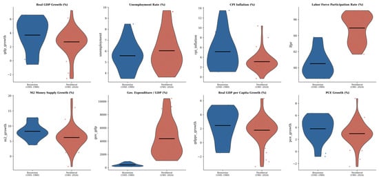
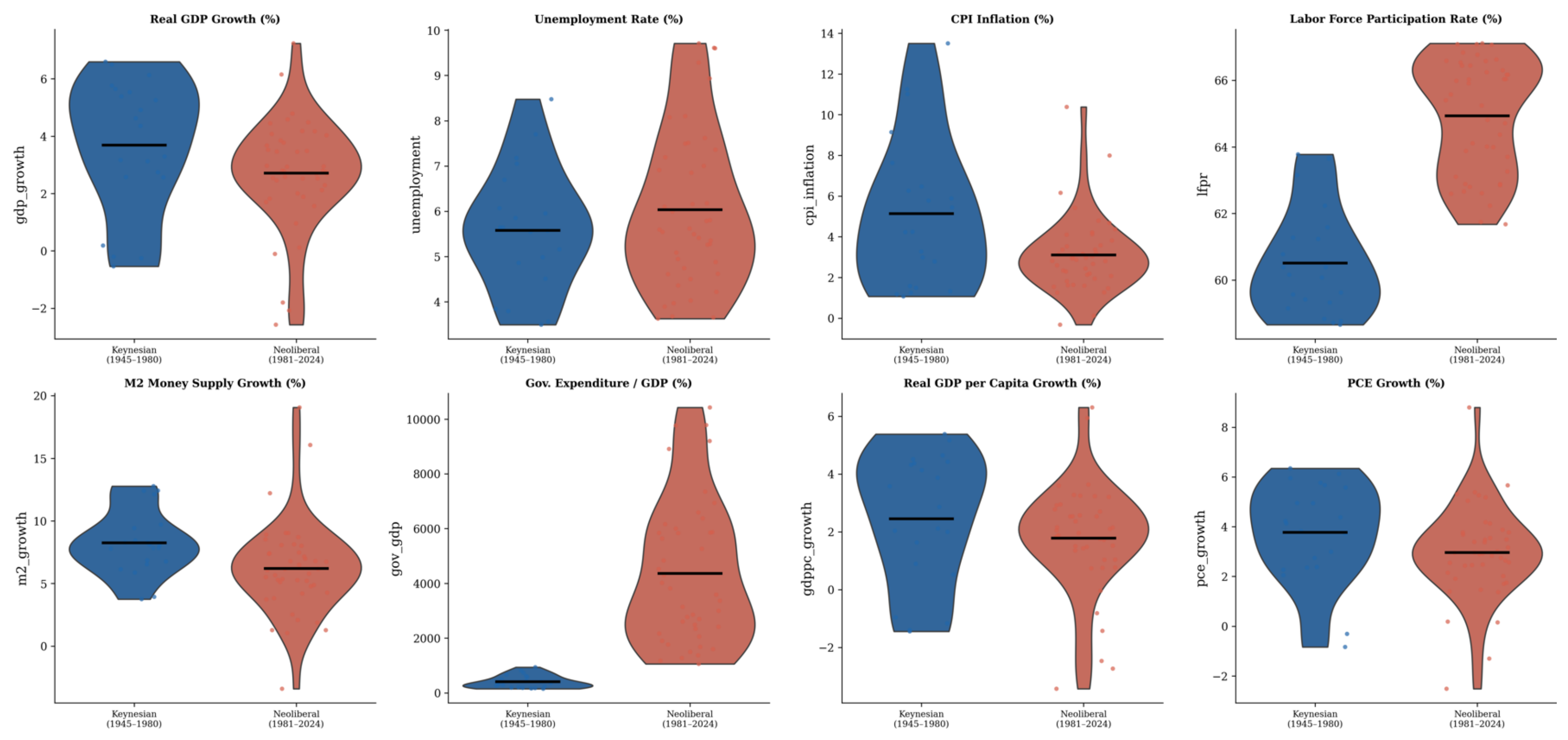
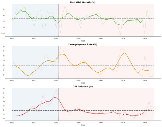
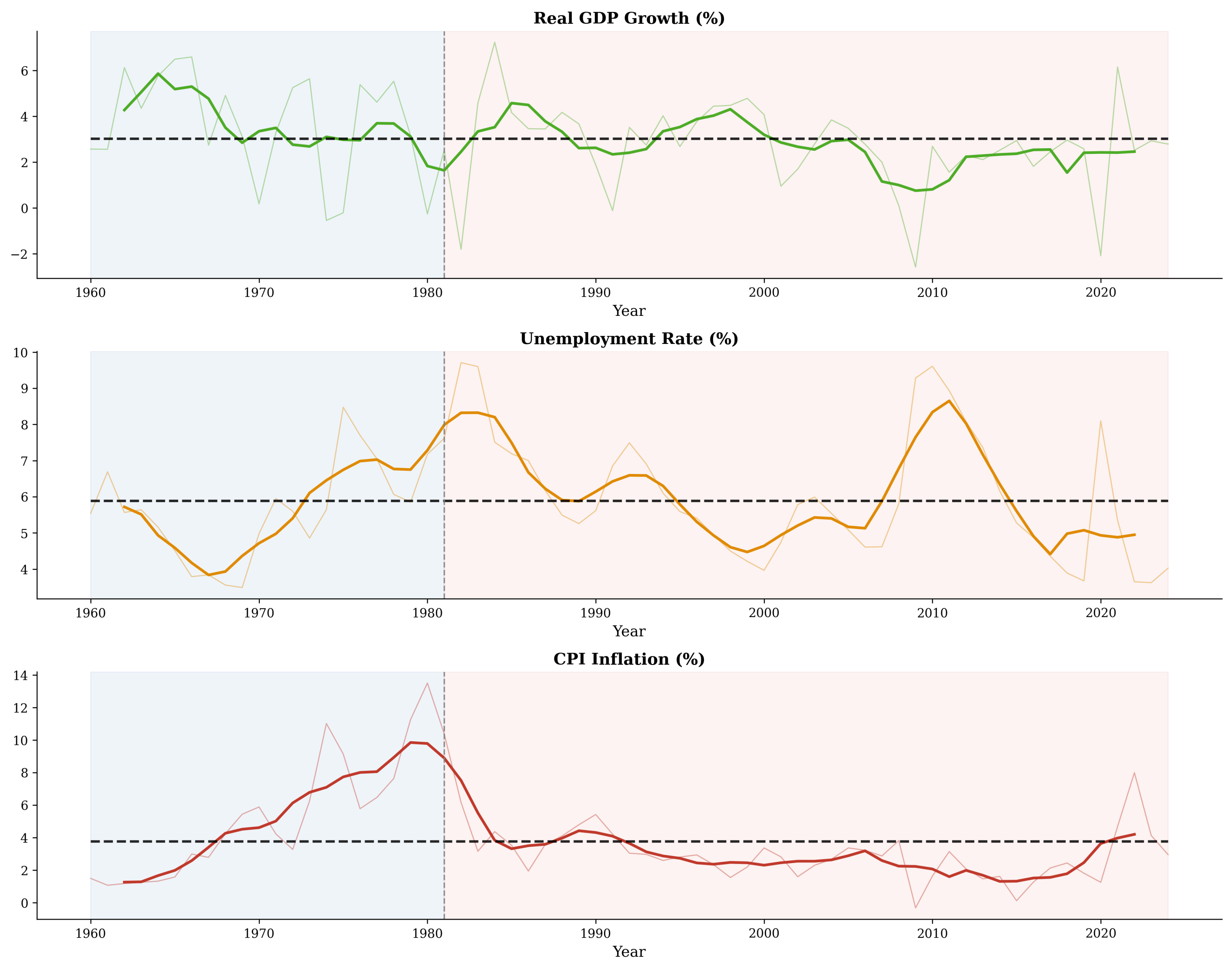
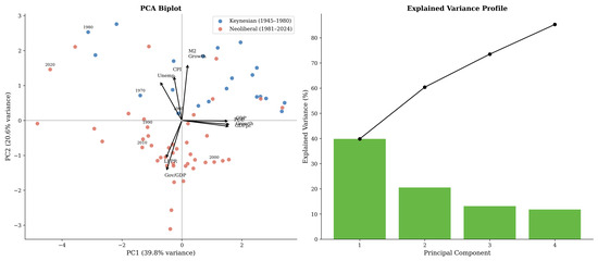
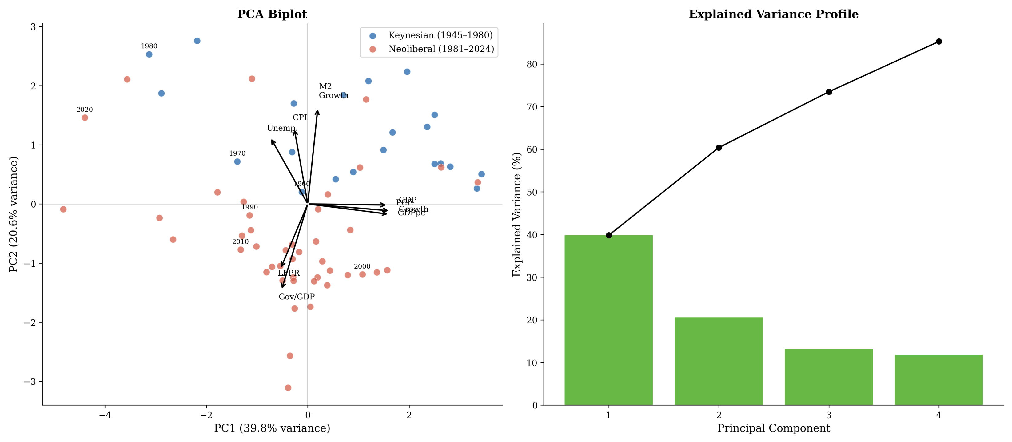
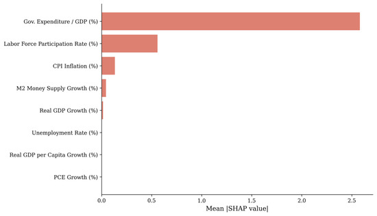
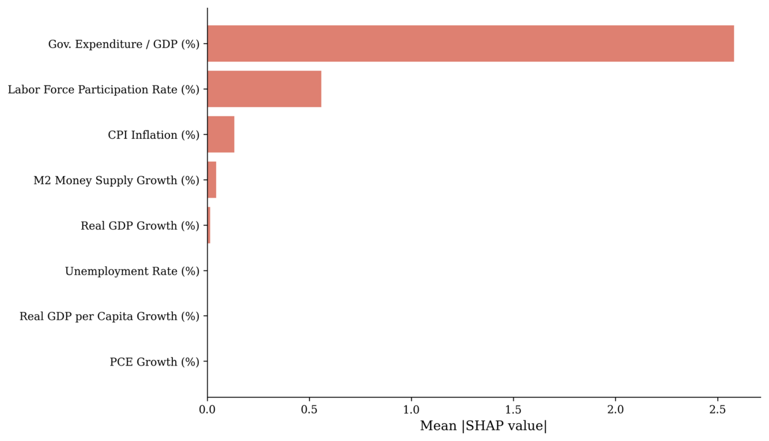
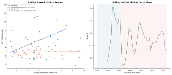
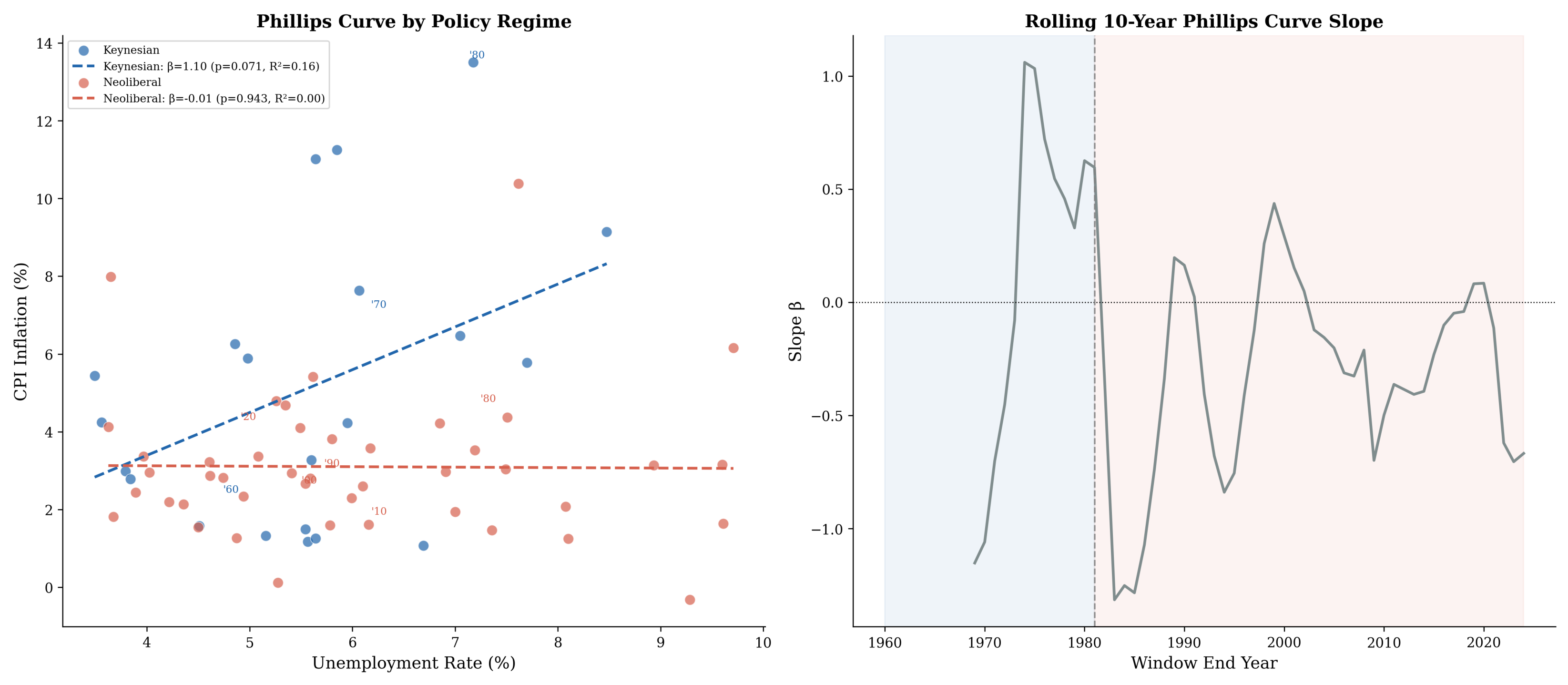
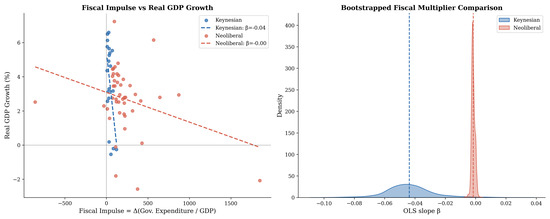
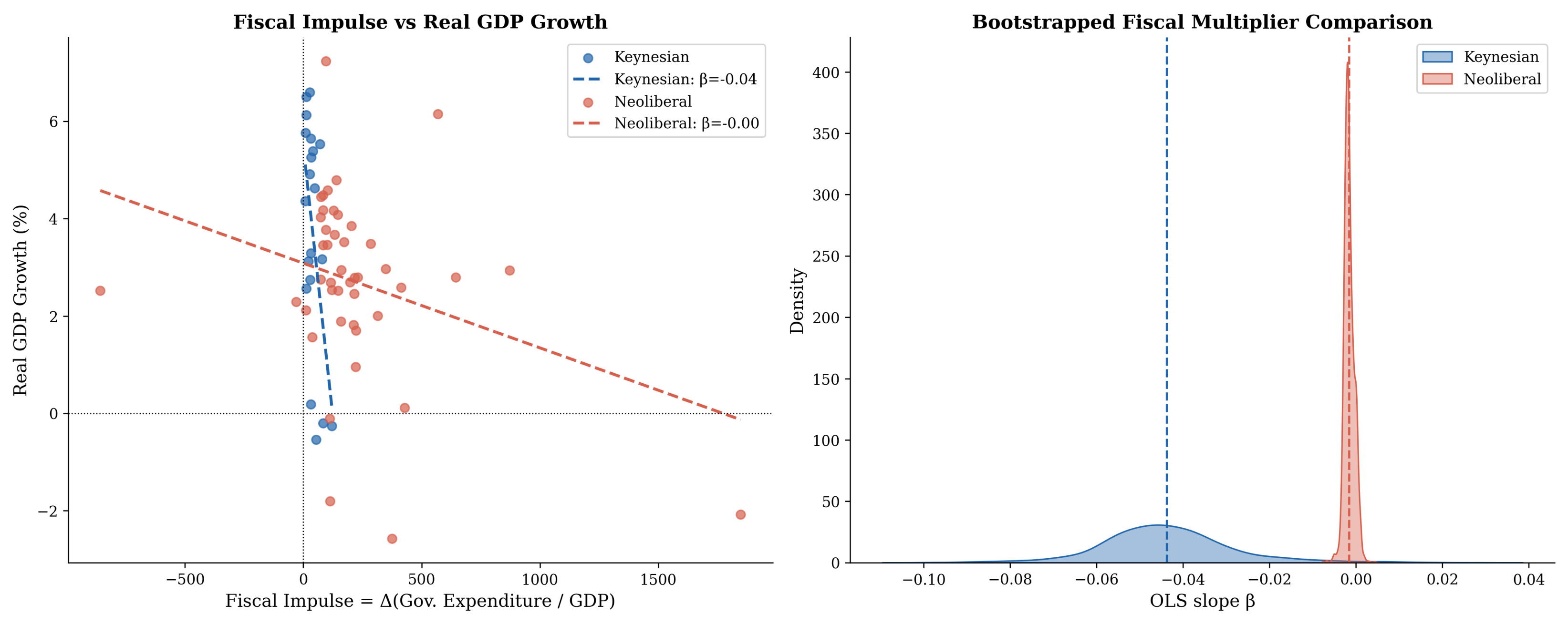
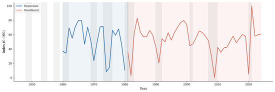
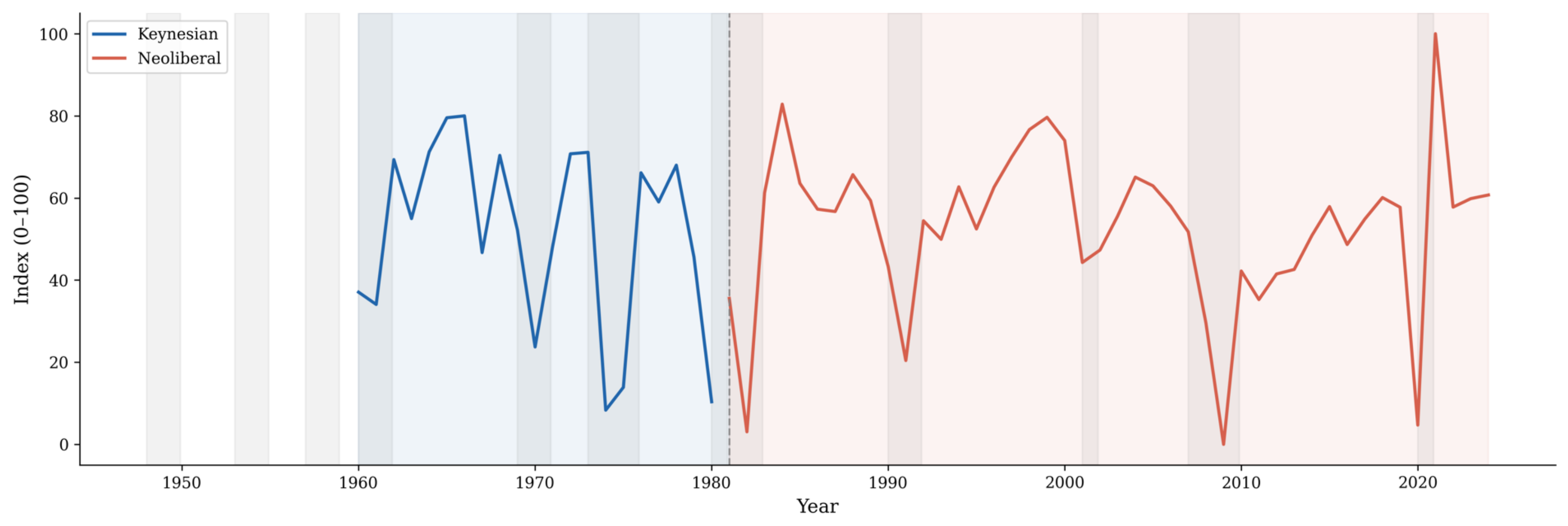
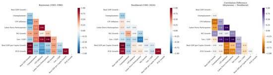
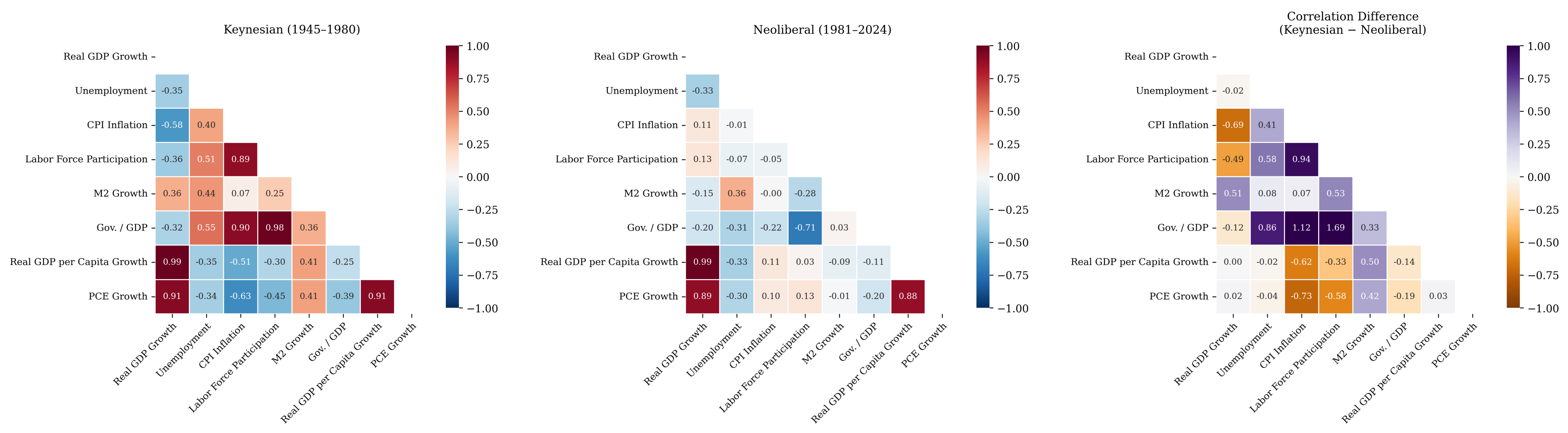
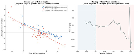
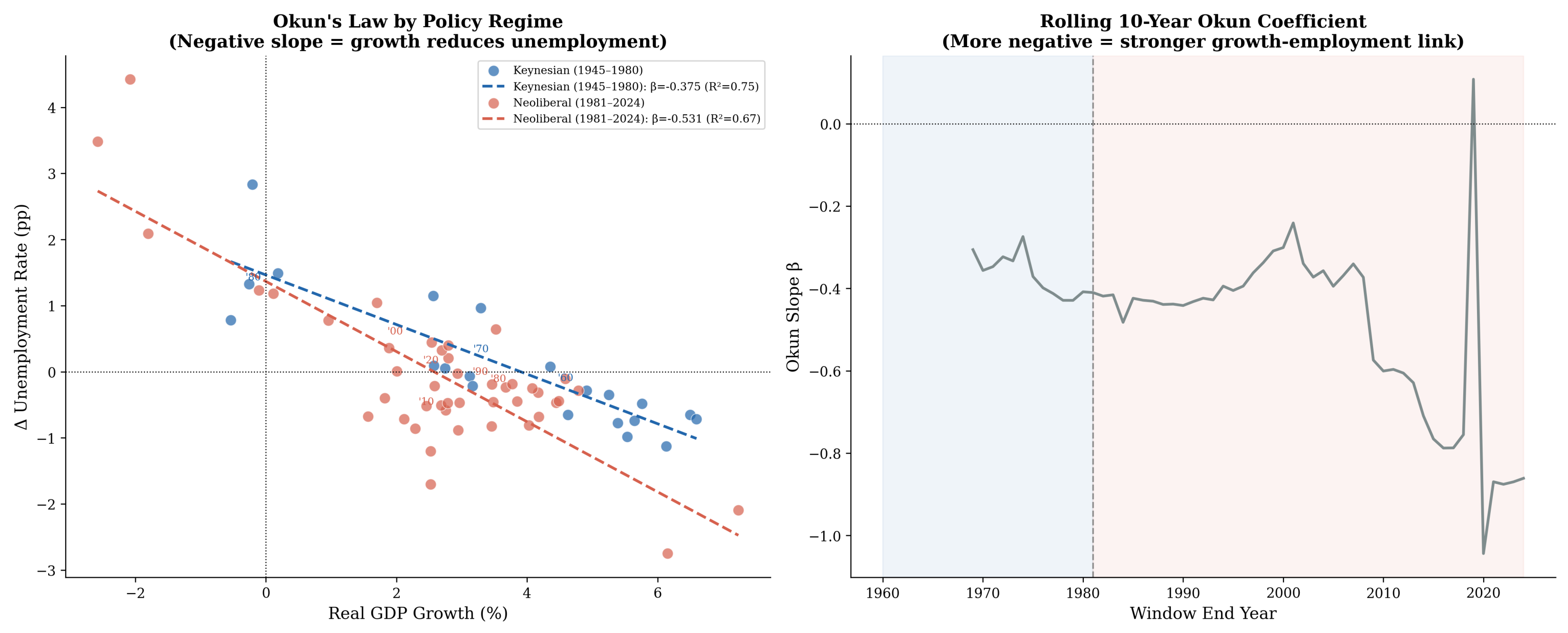
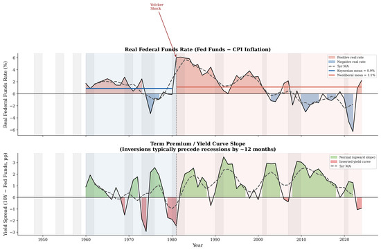
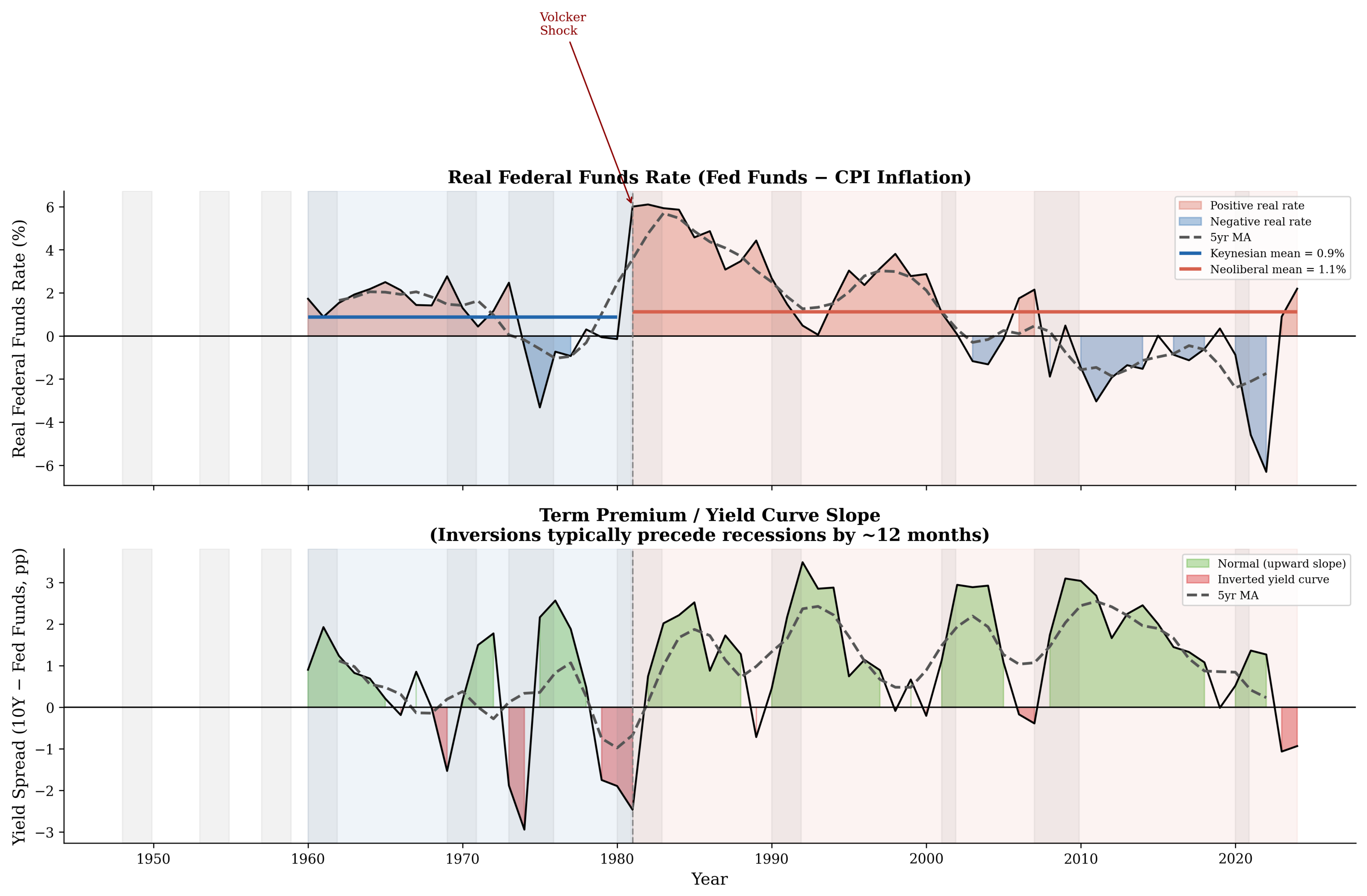
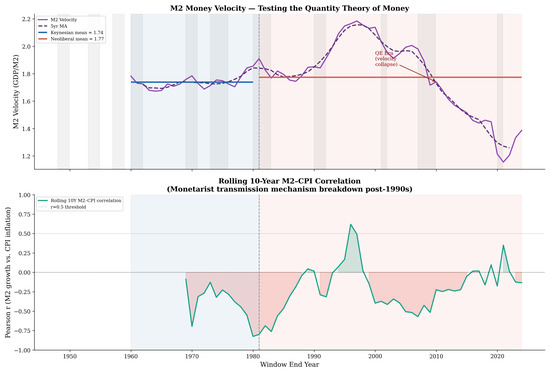
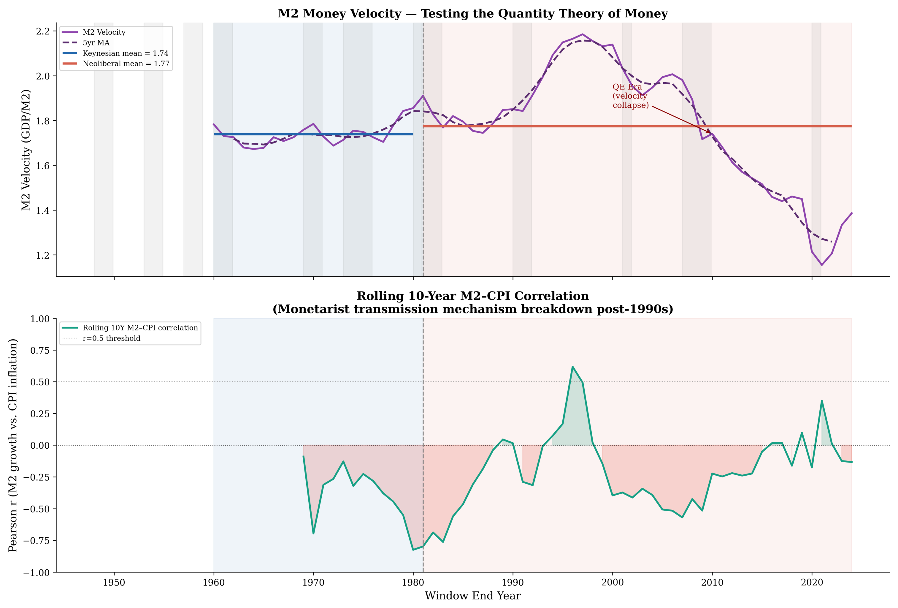
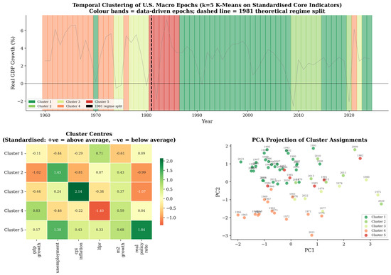
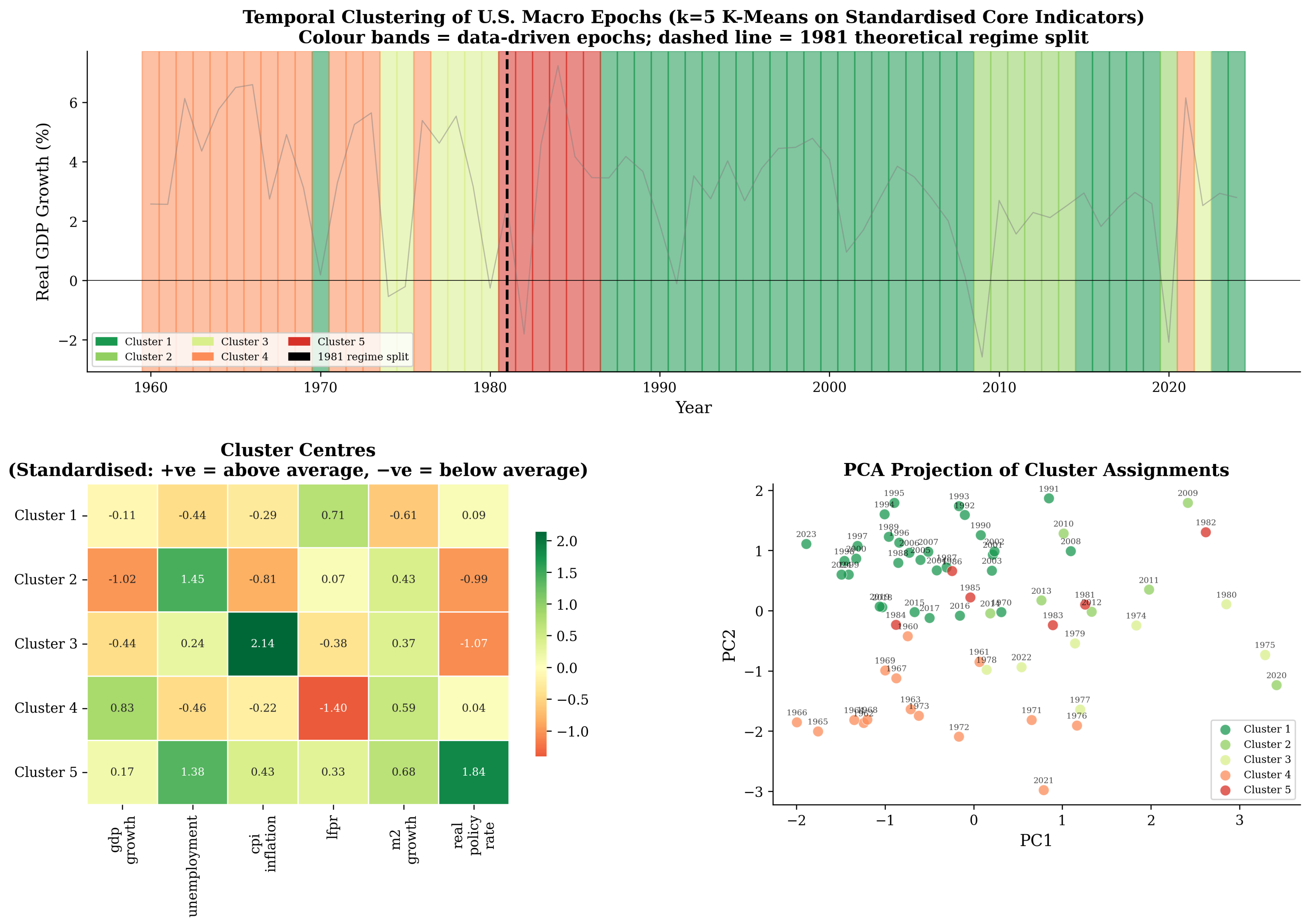
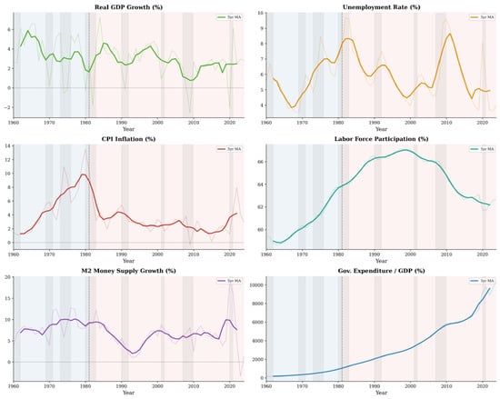
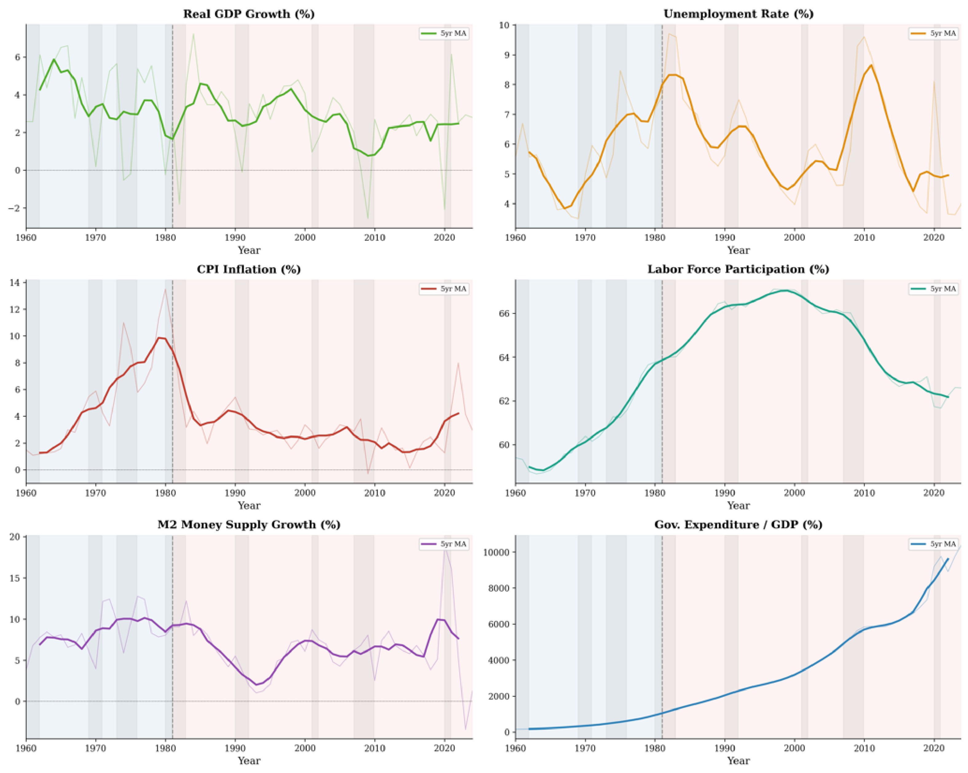
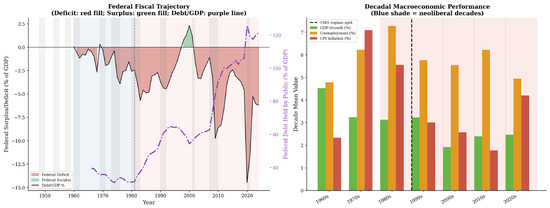
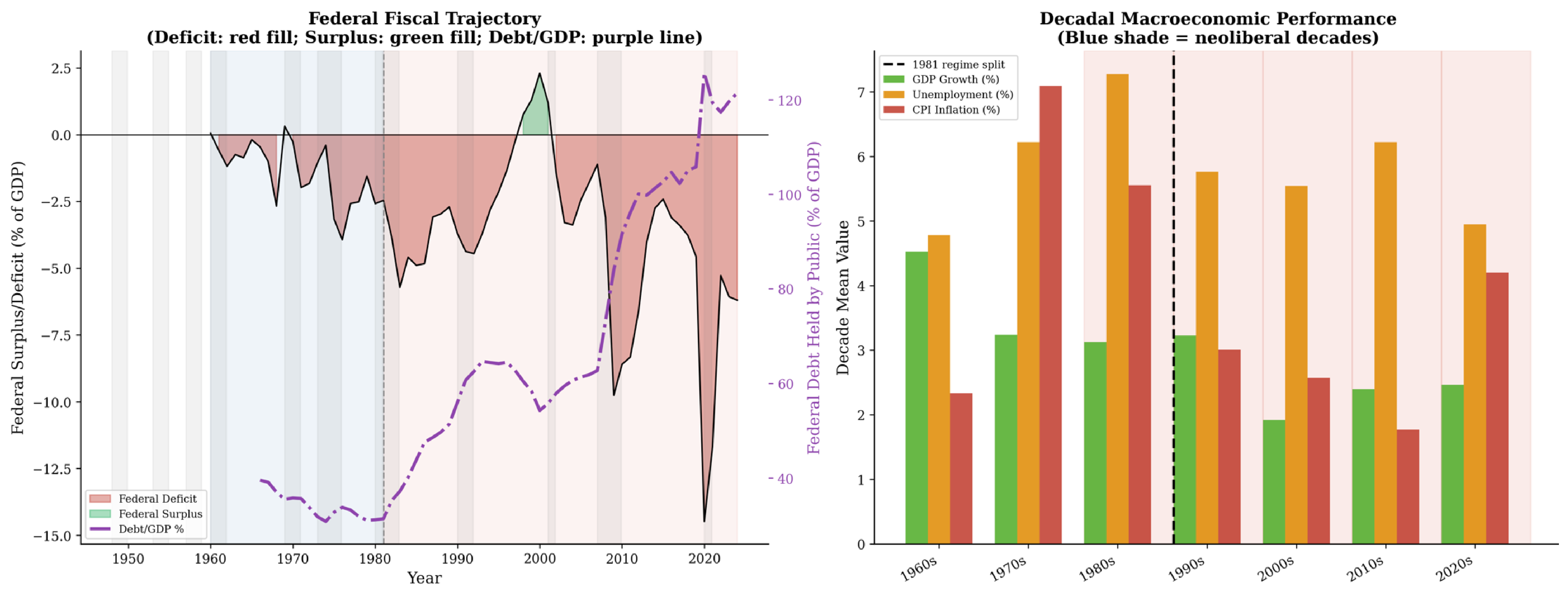
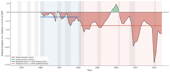
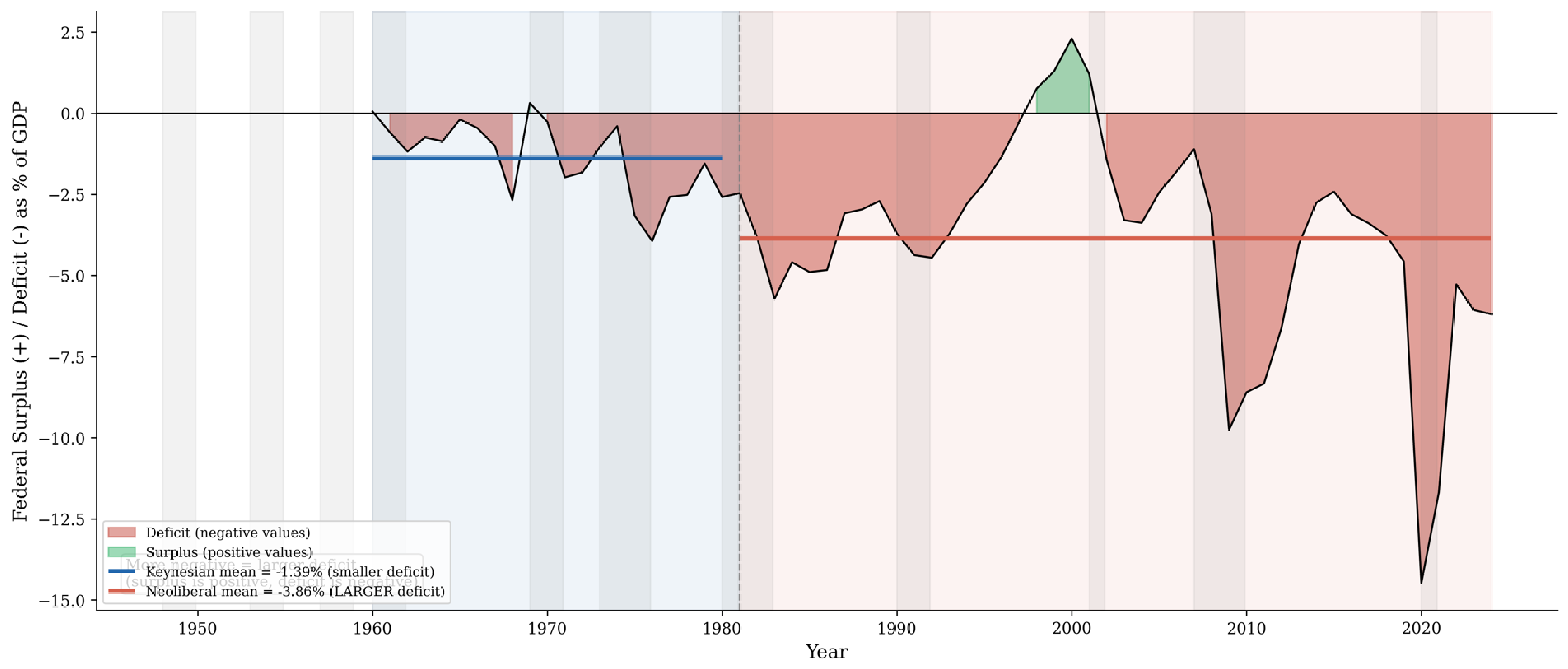
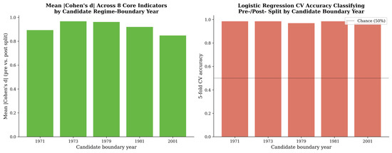
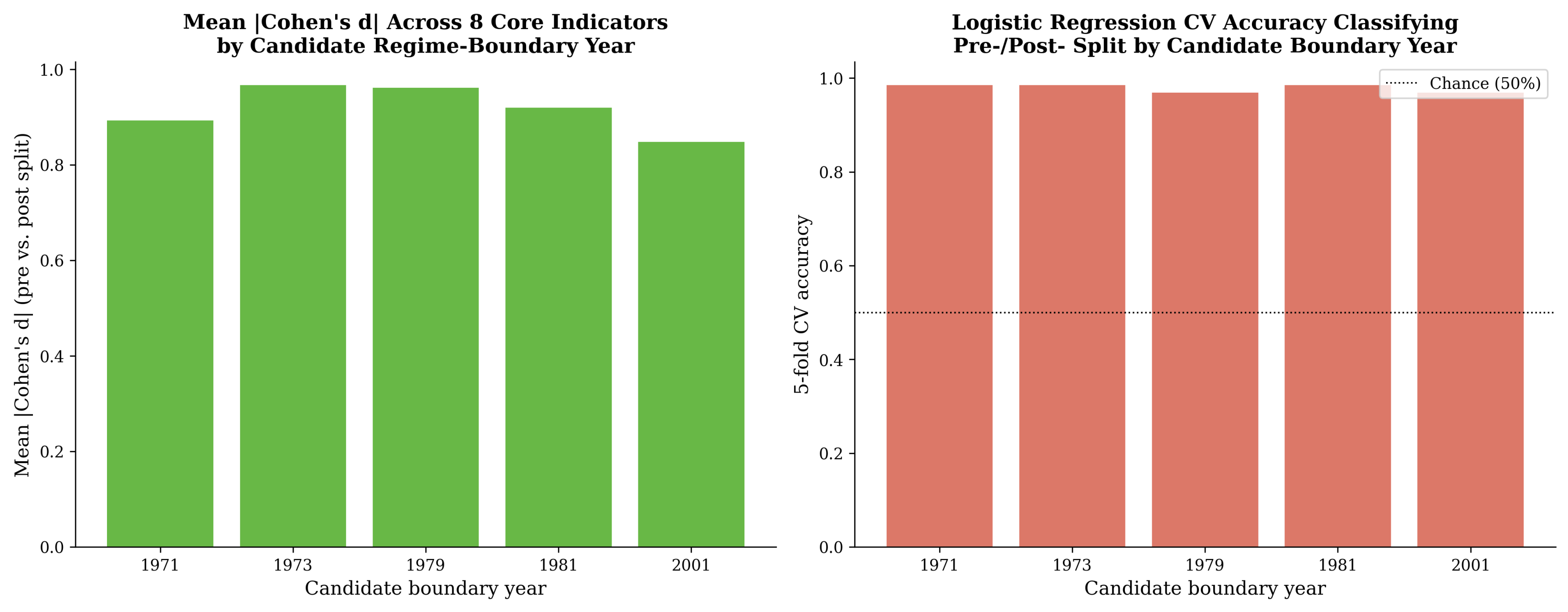
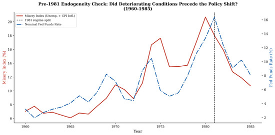
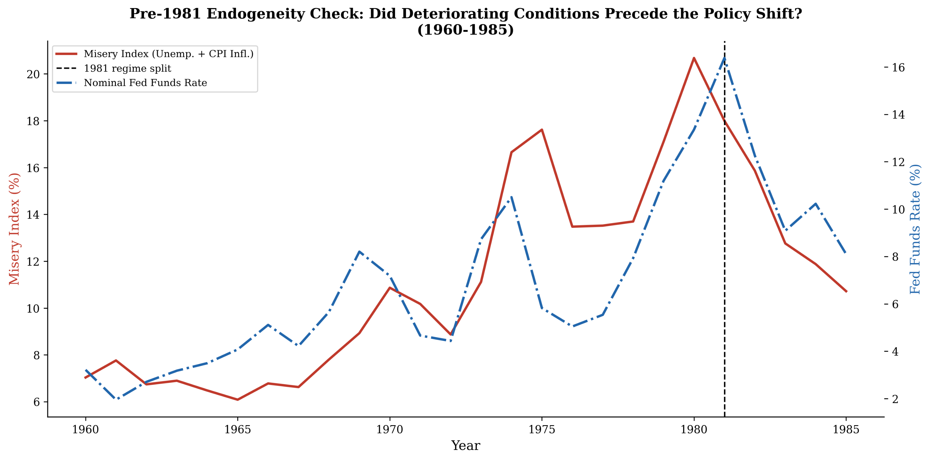
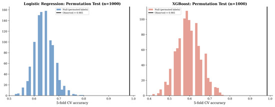
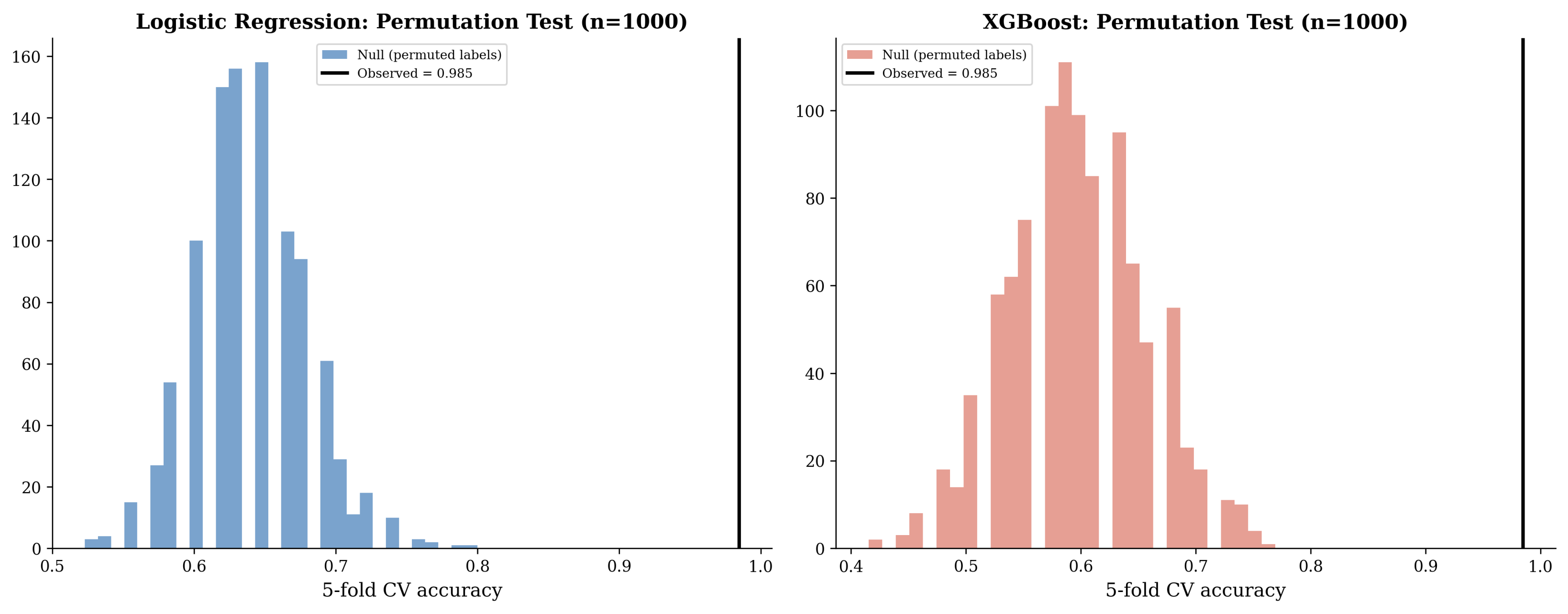
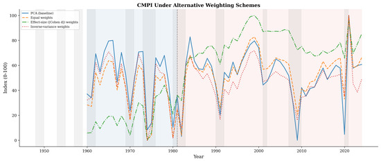
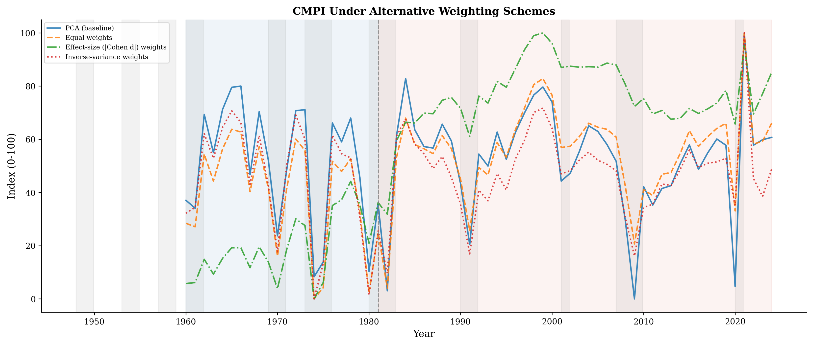
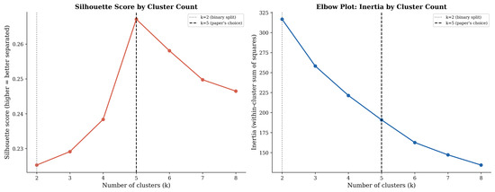
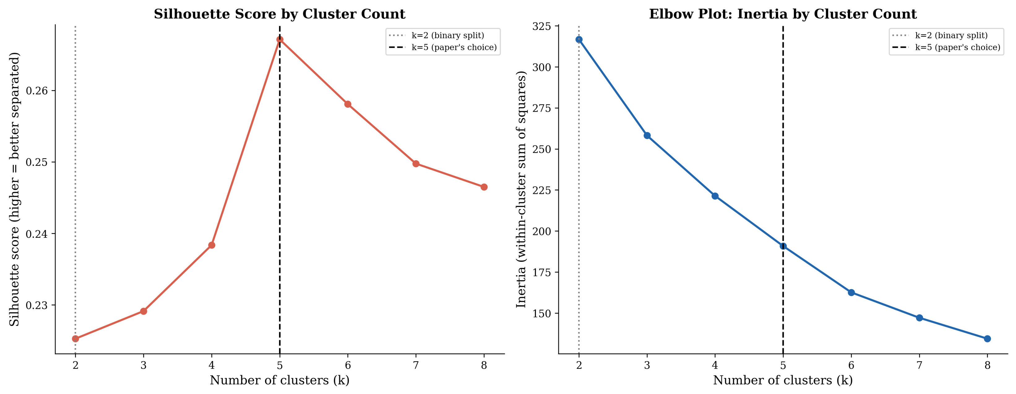
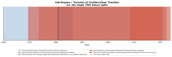
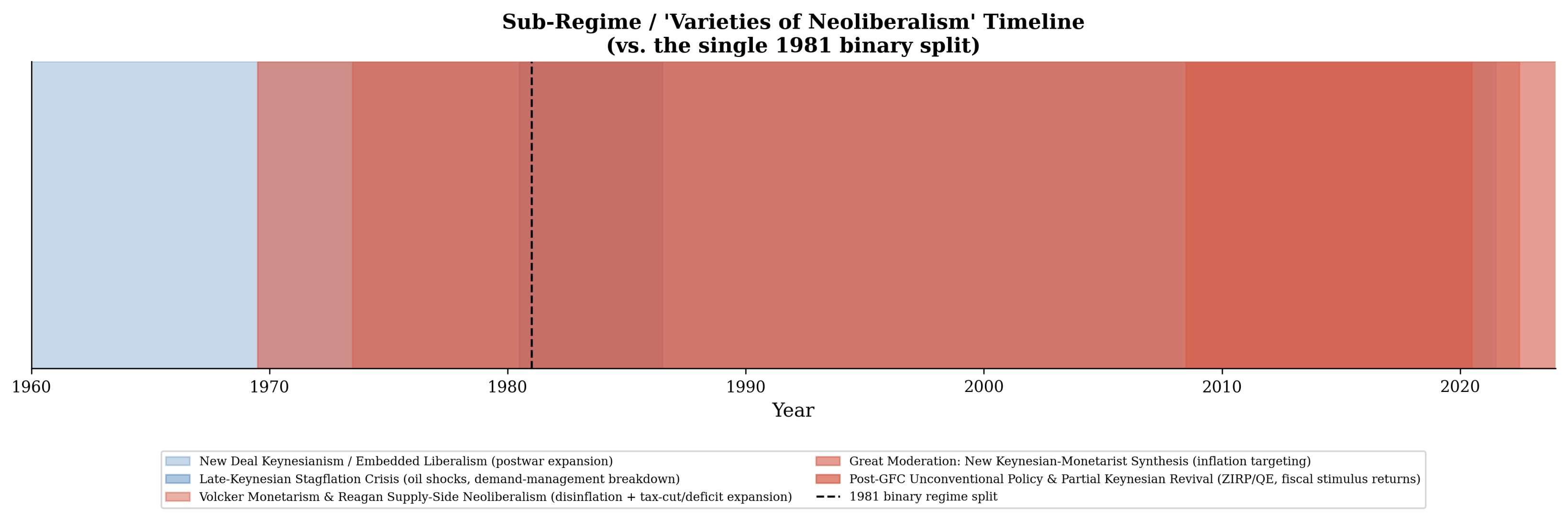

Disclaimer/Publisher’s Note: The statements, opinions and data contained in all publications are solely those of the individual author(s) and contributor(s) and not of MDPI and/or the editor(s). MDPI and/or the editor(s) disclaim responsibility for any injury to people or property resulting from any ideas, methods, instructions or products referred to in the content. |
© 2026 by the authors. Licensee MDPI, Basel, Switzerland. This article is an open access article distributed under the terms and conditions of the Creative Commons Attribution (CC BY) license.