


Abstract
Geopolitical shocks affect small open economies through multiple, correlated channels, yet applied CGE analyses typically impose the timing and persistence of those shocks by assumption. This paper develops a two-stage SVAR–CGE framework that links econometrically identified shock dynamics to general-equilibrium welfare evaluation for Thailand. First, a seven-variable narrative SVAR estimated on monthly data for 2000–2025, identified using the Caldara–Iacoviello Geopolitical Risk Index, is used to recover the persistence of five transmission channels: oil prices, shipping costs, exchange rates, tourism demand, and private investment. Second, these estimated persistence parameters discipline the shock paths in a 22-sector recursive comparative-static CGE model calibrated to Thailand’s 2025 Social Accounting Matrix and simulated over three annual periods using a present-value integral transformation. Under the baseline shock bundle, GDP declines by 3.18% and CPI increases by 5.49%, with welfare losses exhibiting a bimodal distributional pattern—largest for Q1 through consumption-share exposure and for Q4 through tradeable-sector intensity—departing from the monotonically regressive pattern in single-channel analyses. Policy simulations show that targeted transfers calibrated to income rank dominate a universal fuel subsidy on fiscal efficiency, welfare effectiveness (welfare multiplier 1.377 vs. 0.334), and progressivity (1.00 vs. 0.94), at half the fiscal cost (1.48% vs. 2.97% of baseline GDP). An additional bimodal-targeting scenario (S4) at identical fiscal cost underperforms income-rank targeting on all metrics, confirming the latter as the robust second-best instrument under LES preferences with strong MPC heterogeneity. These rankings are supported by the central calibration of a 9-point sensitivity grid, with partial corroboration at off-baseline configurations. The paper contributes by showing that empirically disciplining inter-annual shock dynamics in CGE analysis can materially alter policy conclusions under correlated multi-channel external shocks, shifting the preferred response from sector-specific price subsidies toward demand-side household transfers.
1. Introduction
On 28 February 2026, US–Israeli military strikes against Iran triggered the effective closure of the Strait of Hormuz—through which approximately 20 percent of the world’s oil transits (International Energy Agency, 2026); Brent crude exceeded $100 per barrel by mid-March 2026. Prior simulations of US–Iran conflict scenarios using the War Oil Crisis (WOC) Simulator projected oil price increases ranging from 50% under low-intensity conflict to over 100% under high-intensity scenarios, starting from a baseline of USD 58 per barrel (Ruiz Estrada et al., 2020); the 2026 episode exceeded the upper bound of these projections within the first month. For Thailand, which imports nearly 80 percent of its crude oil and relies on natural gas for two-thirds of its electricity generation, the shock extends well beyond an energy-price disturbance: it simultaneously activates shipping disruptions, exchange-rate depreciation, tourism contraction, and investment uncertainty—and the structural distinction between oil and gas price transmission matters for channel design. Evidence from energy-dependent Gulf Cooperation Council (GCC) economies—where geopolitical proximity to conflict zones amplifies cross-market spillovers—confirms that natural gas price shocks transmit through different financial and commodity channels than oil price shocks, with spillover intensity varying by market and episode type (Al-Maadid et al., 2026). This heterogeneity motivates the present paper’s channel-specific treatment of energy shocks rather than a composite energy-price index that obscures the distinct propagation paths of oil and gas disturbances.
Beyond this technical motivation, the economic burden of this compound disturbance is unlikely to be uniform across sectors, factors of production, and household groups—raising the central questions this paper addresses: how the shock propagates through each channel, how its costs are distributed, and which policy instruments most efficiently limit welfare losses.
A key structural feature of compound geopolitical shocks is that their constituent channels differ substantially in timing, persistence, and decay rate. Energy-cost effects emerge within weeks; exchange-rate pass-through to consumer prices may take months; and investment responses operate with a longer lag still, as firms revise capital-expenditure plans in response to sustained uncertainty. The observed 3–6% depreciation of the Thai baht against the US dollar in the weeks following the onset of the conflict (Bank of Thailand, 2026) illustrates the speed of the financial channel relative to the real economy. These cross-channel differences imply that the aggregate welfare impact cannot be assessed from static or single-channel analyses: what matters for policy design is not only the initial magnitude of the disturbance but also how quickly each channel decays and how long its effects persist.
A growing literature links geopolitical uncertainty to oil-market disruptions, financial-market volatility, and investment contractions, with effects documented to be severe for commodity-importing, trade-dependent economies (Caldara & Iacoviello, 2022). A parallel strand of CGE-based research has evaluated the economy-wide and distributional consequences of energy-price increases. These two literature; however, remain weakly integrated: time-series studies identify shock dynamics without tracing sectoral and welfare incidence, while CGE studies model propagation without empirically disciplining shock timing and persistence.
Beyond this integration gap, two important limitations persist in the existing literature. First, empirical analyses of geopolitical shocks in emerging economies remain predominantly focused on the oil-price channel, with comparatively limited attention to the simultaneous transmission through shipping costs, exchange-rate adjustment, tourism demand, investment expectations, and input-cost pass-through. Studies that do address multiple channels typically treat them in isolation rather than within a unified framework, making it difficult to assess their relative magnitudes and interactions. Second, and more critically for dynamic policy analysis, CGE-based assessments of external shocks almost invariably impose the persistence and decay structure of shocks exogenously. The assumed rate at which a shock dissipates over time is rarely estimated from historical data, even though it can materially alter simulated outcomes for GDP, sectoral output, investment, and household welfare. As a result, recursive comparative-static simulation studies often rely on arbitrary persistence assumptions that reduce the empirical credibility of their inter-annual shock profiles.
This paper asks three research questions. First, how do geopolitical oil-price and shipping-cost shocks propagate through Thailand’s exchange rate, tourism, and investment channels, and what are their relative magnitudes? Second, how persistent are these transmission effects, and what implications do estimated persistence parameters have for disciplining the inter-annual shock paths in a recursive comparative-static CGE simulation? Third, how do multi-channel external shocks affect macroeconomic aggregates, sectoral output, and household welfare across the expenditure distribution?
To answer these questions, the paper develops a two-stage empirical framework. In the first stage, a Narrative Structural Vector Autoregression (SVAR) is estimated over January 2000–December 2025, using the Caldara–Iacoviello Geopolitical Risk (GPR) Index to identify the dynamic responses of Thailand’s key macroeconomic variables—producer prices, consumer prices, and the exchange rate—to external oil-price and shipping-cost shocks. A critical identification distinction governs how the SVAR output is used. The 2026 geopolitical episode exceeds the historical range of GPR observations used in estimation; accordingly, the SVAR does not determine the magnitude of the 2026 shock, which is instead calibrated directly from observed 2026 data using narrative identification in the tradition of Romer and Romer (2004). What the SVAR supplies is the temporal decay structure—the speed, lag profile, and persistence of each identified transmission channel—derived from the full distribution of historical geopolitical episodes in the estimation sample. This separation between shock magnitude (calibrated from the 2026 episode) and shock persistence (estimated from historical dynamics) is the key methodological feature that prevents the counterfactual simulation from depending on the arbitrary assumption that a crisis of unprecedented scale decays at a historically average rate. Three operational roles follow from this separation: the SVAR identifies the relative timing, persistence, and transmission hierarchy of shocks across channels; scenario magnitudes are calibrated from observed 2026 market conditions; and the CGE model translates these disciplined shock paths into sectoral and household welfare outcomes.
This paper’s contribution is to discipline inter-annual shock dynamics in CGE analysis using empirically derived persistence structures. Three dimensions elaborate on this contribution. First, the SVAR supplies an econometrically disciplined persistence and transmission structure: a data-validated causal hierarchy of channels (primitive vs. propagated), a genuine SVAR-estimated persistence for the investment channel (), and an empirically grounded lower bound () for the remaining four channels derived from minimum observed geopolitical episode durations—reducing arbitrariness in shock profiling without overstating what the SVAR can deliver for tail episodes. Second, the analysis incorporates shipping costs, exchange-rate adjustment, tourism demand, and investment responses alongside oil prices within a unified framework, allowing their relative magnitudes and interactions to be assessed simultaneously rather than in isolation. Third, by incorporating five expenditure quintiles, the paper documents a bimodal distributional incidence pattern—Q1 most exposed through consumption-share effects and Q4 through tradeable-intensity effects—that departs from the monotonically regressive pattern in prior single-channel analyses (Jongwanich & Park, 2011; Warr, 2008), and derives transfer design implications from the empirically identified rather than assumed incidence profile.
1.1. What Time-Series and SVAR Studies Can Do—And Where They Stop
The macroeconomic literature on geopolitical risk has established three robust findings. Geopolitical disturbances generate compound external shocks whose consequences depend critically on their source: Baumeister and Kilian (2016) show that supply-driven and demand-driven oil price movements produce different macroeconomic outcomes; Kilian and Murphy (2014) and Kilian (2009) establish that geopolitical supply disruptions compress output and raise inflation simultaneously in net-importing economies. Mahmoudinia et al. (2025) confirm the principle in an SVAR context closely analogous to the present study: separating oil structural shocks and tracing their impulse responses through food and non-food prices demonstrates that shock extraction from data, prior to downstream simulation, is essential for credible welfare analysis. Building on this shock-identification tradition, the Caldara and Iacoviello (2022) GPR Index documents that geopolitical risk spikes generate significant declines in real activity and investment, with non-linear amplification during actual conflict episodes; cross-quantilogram evidence confirms that GPR–commodity price linkages strengthen substantially during high-volatility periods (Liu et al., 2025).
More recently, the Russia–Ukraine conflict demonstrated that geopolitical disturbances transmit through multiple simultaneous pathways: an energy-price channel raising production costs and inflation (Lippi & Nobili, 2012; Sun et al., 2024); a supply-chain and logistics channel propagating through production networks conditioned on supplier diversification (Joyez, 2025); and an uncertainty and financial-spillover channel generating heterogeneous cross-market volatility (Chowdhury et al., 2025; Shang & Hamori, 2025). These pathways are interdependent: energy price increases raise logistics costs, logistics disruptions constrain trade adjustment, and uncertainty amplifies cross-market volatility. Their aggregate effect therefore depends on joint configuration rather than on channel-by-channel magnitudes.
These multi-channel features extend directly to the Thai case. For Thailand specifically, the structure engages five transmission mechanisms with distinct adjustment speeds: energy costs (weeks), exchange-rate pass-through (months), shipping and supply-chain disruptions (concurrent with trade), tourism demand (lagged by security perception), and private investment (delayed by capital-expenditure revision). Jongwanich and Park (2011) document that commodity price shocks disproportionately burden lower-income Thai households, while Warr and Kohpaiboon (2007) provide the foundational CGE analysis of external price shocks for Thailand on which the present study builds.
The limitation of this literature is not in shock identification but in its downstream reach. Time-series and SVAR studies identify persistence, transmission hierarchy, and channel magnitudes with precision—but do not by themselves trace identified shocks through sectoral structures and household welfare distributions. The persistence parameters remain in the econometric system; they do not discipline the structural simulations that would be needed to evaluate policy.
1.2. What CGE Studies Can Do—And Where They Stop
The computable general equilibrium framework fills this gap in distribution and propagation. Following Lofgren et al. (2002), CGE models decompose aggregate welfare effects into equivalent variation by household group, tracing the transmission chain from shock through sectoral output, factor returns, and household income to quintile-level welfare outcomes. Prior CGE work establishes that external shocks generate heterogeneous welfare incidence shaped by market structure, expenditure patterns, and factor market flexibility (Diao & Kennedy, 2016; Mukashov et al., 2026; Somé & Zidouemba, 2025). For ASEAN economies, evidence consistently documents regressive commodity-shock incidence driven by food and energy expenditure shares (Imai et al., 2014; Warr, 2008), with targeted transfer programmes outperforming universal fuel subsidies on fiscal efficiency and distributional grounds (Coady et al., 2019; World Bank, 2022).
The limitation of CGE-based assessments is not in propagation mechanics—which are well-developed—but in the treatment of the shock itself. Recursive CGE studies are designed to trace inter-annual adjustment paths, yet the persistence and decay structure of the exogenous disturbance are overwhelmingly imposed by scenario design rather than identified from data. Sun et al. (2025) specify short-, medium-, and long-run scenarios without empirical discipline on shock persistence; Sun et al. (2024) impose scenario blocks from external assumption; and Wing (2008), Antimiani et al. (2013), and Hosoe et al. (2010) calibrate shock persistence to historical averages rather than to episode-specific dynamics. Even the systematic risk profiling framework of Mukashov et al. (2026)—which explicitly criticises ad hoc scenario analysis—improves shock attribution without disciplining temporal shock evolution through an external macroeconometric system.
The consequence is material. A front-loaded oil shock, a hump-shaped uncertainty response, and a long-lived volatility disturbance are treated identically under assumption-based calibration. Yet these three profiles produce different inter-annual consequences for capital accumulation, sectoral adjustment, and welfare incidence once timing differs.
1.3. The Missing Link—And What This Paper Does
Existing studies either identify macro shocks without welfare analysis or evaluate welfare without empirically grounded shock dynamics. This paper bridges these two strands by introducing a framework that uses empirically derived persistence structures to discipline inter-annual CGE simulations under multi-channel geopolitical disturbances—one that is honest about the limits of identification for tail events while still delivering more credible shock profiles than pure assumption.
To the authors’ knowledge, no published study has applied SVAR-derived AR(1) persistence parameters to discipline inter-annual shock decay in a recursive dynamic CGE model calibrated to a developing-country SAM under a correlated multi-channel geopolitical disturbance. This study situates this claim against three nearby strands rather than as a universal priority statement. Dynamic global CGE models—McKibbin and Wilcoxen’s G-Cubed (McKibbin & Wilcoxen, 1999) and GTAP-Dyn (Hertel et al., 2007; Ianchovichina & Walmsley, 2012)—embed persistence through forward-looking expectations or capital accumulation, not through externally estimated channel-specific . Mukashov et al. (2026) improve shock attribution; the present paper complements this by disciplining shock decay paths. Elberry et al. (2026) and Koutsandreas et al. (2026) soft-link CGE to energy systems models; this analysis uses a macroeconometric system instead. The specific gap is the operational use of channel-specific SVAR persistence parameters as the linkage variable in recursive dynamic CGE simulation under multi-channel external transmission for a developing-country case.
The use of SVAR output to discipline subsequent structural models—rather than as a standalone forecasting exercise—follows a developing literature on SVAR-calibrated structural frameworks for advanced economies (Berger & Vavra, 2015; Fornaro & Wolf, 2023); the present paper extends this approach to a geopolitical episode in a developing economy, where the external source of discipline is persistence structure rather than demand estimation. Related model-linking studies establish architectural feasibility without providing this linkage: Elberry et al. (2026) and Koutsandreas et al. (2026) connect CGE models to externally generated information, but their external source is a technology-rich energy model rather than an econometric system identifying macroeconomic shock dynamics.
A tail-event identification concern merits acknowledgment. The 2026 Strait of Hormuz closure has no direct historical precedent in the SVAR estimation sample. The two-step design addresses this: persistence parameters are estimated from the full 2000M01–2025M12 sample spanning episodes of varying severity, while initial shock magnitudes are calibrated to observed 2026 data (Brent above $100, BDI surge, baht depreciation of approximately 3–6% since the onset of the conflict). The result is not an SVAR forecast but a structured simulation in which the SVAR reduces arbitrariness in the inter-annual shock profile while observed event data anchor its initial scale.
2. Materials and Methods
To make the econometric-discipline status of each transmission channel visible before the methodological development that follows, this study summarises the five-channel architecture in Table 1. The table distinguishes SVAR-identified channels, whose persistence parameter is taken directly from the SVAR output (subject to the floor adjustment described in Section 2.1), from SVAR-validated channels, whose empirical relevance is confirmed by FEVD but whose Year-1 magnitude is calibrated from observed 2026 event data. A formal decision rule defining the boundary appears in Section 2.3.
Table 1.
Five-channel summary: persistence, magnitude source, and identification status.
This study estimates a narrative Structural Vector Autoregression (SVAR) using the AI-GPR Index of Caldara and Iacoviello (2022) to identify the dynamic responses of key Thai macro-financial variables to geopolitical shocks. The estimated persistence parameters are then transformed into calibrated shock paths and applied across a three-period sequence of comparative-static CGE equilibria, in which each period’s shock magnitude decays according to the SVAR-estimated . This recursive comparative-static design preserves inter-annual shock dynamics without requiring an intertemporal optimisation framework (Figure 1).
Figure 1.
Two-stage SVAR–CGE framework for geopolitical shock transmission in Thailand.
2.1. Narrative Structural Vector Autoregression with AI-GPR Identification
2.1.1. Reduced-Form Specification
A seven-variable VAR is estimated on monthly data over 2000M01–2025M12 (311 observations). Lag length is selected following Kilian and Lütkepohl (2017), who recommend a minimum of three lags at monthly frequency to avoid residual autocorrelation; information criteria and diagnostics are reported in Appendix B.1. The vector comprises the AI-GPR Index, log-differenced Brent crude, the Baltic Dry Index, the THB/USD exchange rate, PPI year-on-year inflation, log-differenced tourist arrivals, and private investment growth. GPR is the identifying instrument; PPI is retained as a cost pass-through control. Full specification and stationarity tests are in Appendix B.1.
2.1.2. Structural Identification
Structural shocks are identified via a recursive Cholesky decomposition (Hamilton, 1994; Sims, 1980) with the ordering GPR → OIL → BDI → EXR → PPI → TOUR → INV, reflecting Thailand’s small-open-economy position; formal zero restrictions and the structural matrix S are reported in Appendix B.2. The recursive ordering is not innocuous, and this study adopts two robustness strategies. First, permuting all 24 valid middle-block orderings while holding GPR first and OIL–BDI second leaves the estimated values within of the main specification (Appendix B.5). Second, the SVAR identifies persistence rather than magnitude—the 2026 shock magnitude is calibrated from observed event data through narrative identification, shielding the inter-annual shock paths from the most consequential identification risks. Sign-restriction identification (Uhlig, 2005) would provide a further robustness layer; this study does not implement it because the Cholesky-identified impulse responses already exhibit theoretically expected signs at peak horizons for all five CGE channels, suggesting sign restrictions would not meaningfully alter estimated . A formal implementation remains a useful extension. Table 2 reports the estimated persistence parameters and Year-1 peak responses that enter the PV-integral transformation in Section 2.3.2.
Table 2.
SVAR-estimated persistence parameters and Year-1 peak responses.
Year-1 peak magnitudes () are derived via a two-step procedure in which the SVAR supplies the IRF shape and the shape is re-scaled to match observed 2026 market movements—Brent %, BDI %, THB/USD %—consistent with Romer and Romer (2004); re-scaling details and magnitude sensitivity appear in Appendix B.4 and Section 3.5, respectively. Persistence parameters are estimated from log-linear IRF decay between and , with a floor is applied when any of three conditions hold: (i) raw ; (ii) IRF sign reversal between peak and ; or (iii) peak IRF magnitude negligibly small (<), making the ratio unreliable. Condition (iii) is operative for BDI → INV, corresponding to a half-life of approximately 2.5 months. Two channels receive non-standard treatment: follows a Dornbusch overshooting prior (Dornbusch, 1976) in place of the floor, motivated by the near-zero contemporaneous response arising from the Cholesky ordering; and is FEVD-weighted across the , , and channels, reflecting the delayed and compounding nature of investment responses. Raw estimates and floor-sensitivity results are reported in Appendix B.3 and Section 3.6.
2.1.3. Role of the SVAR in the Two-Stage Framework
The SVAR supplies persistence parameters and the shock hierarchy (Table 3) that govern how calibrated Year-1 magnitudes propagate across simulation years. The annual CGE projection rule is
where is the calibrated Year-1 magnitude and the SVAR-estimated persistence. The monthly IRF decay profile and its PV transformation are developed in Section 2.3.2.
Table 3.
Shock hierarchy and CGE entry mode.
Tier A channels (OIL, BDI) enter the CGE as exogenous import price shocks () with no reverse causation from Thai variables, consistent with their Cholesky ordering. Tier B channels (EXR, TOUR, INV) enter with SVAR-derived persistence multipliers, reflecting significant IRF responses to Tier-A shocks at –12 months. The anti-double-counting property is maintained throughout: no variable appears simultaneously in both the calibration-magnitude role and the SVAR-persistence role. A full decomposition of the four analytical functions the SVAR performs—shock hierarchy identification, lag-structure estimation, five-channel validation via FEVD, and anti-double-counting audit—is provided in Appendix B.6.
2.2. Comparative-Static CGE Model
2.2.1. Social Accounting Matrix
The CGE model is calibrated to a 22-sector Thailand SAM for base year 2025, constructed from the Thailand Input-Output Table 2021 (180-sector disaggregation) and balanced against NESDC national accounts via cross-entropy methods (Robinson et al., 2001). Because NESDC publishes national accounts with a one-year lag, the 2025 SAM accounts are forward-projected from the most recent available benchmark year (2024) using GDP growth rates and sectoral price deflators; all macro deviations between the projected 2025 SAM and the 2024 NESDC benchmarks are within pp, confirming numerical stability of the calibration. Specifically, GDP at market prices deviates by 0.68% (THB 18,143 vs. 18,021 billion); private consumption and export shares match to within 0.3 percentage points; and the maximum cell-level imbalance after cross-entropy balancing is below 0.000006. Full validation against 29 macro aggregates appears in Appendix A.1.
The SAM covers 22 production sectors, five household quintiles (Q1–Q5 by per capita expenditure), government, capital, and rest-of-world accounts. Three sectoral shares are central for shock transmission: petroleum and coal (approximately 8.3% of intermediate demand); transport and logistics (4.7% of intermediate use); and tourism and accommodation (8.4% of household expenditure and 12–15% of aggregate exports).
2.2.2. Production, Trade, and Demand
Production follows a nested CES–Leontief technology:
with Leontief intermediate inputs aggregated under value-added. Trade is modelled via Armington (CES import) and CET (export) aggregators with elasticities from GTAP v10 (Appendix A.3), supplemented by sector-specific calibration following Tokarick (2010) for non-tradeable services. Household demand follows a Linear Expenditure System (LES) calibrated to SES 2023 consumption shares. Capital is fixed at the sectoral level (appropriate for single-period analysis), and labour supply is fixed. Model closure fixes the nominal wage () as numeraire and allows sectoral capital rental rates, producer prices, and the exchange rate to clear factor, goods, and external markets, respectively.
2.3. Shock Calibration and PV-Integral Transformation
2.3.1. Five-Channel Shock Bundle
Five empirically disciplined transmission channels correspond to the principal pathways through which geopolitical events reach small open commodity-importing economies: energy costs (OIL), freight costs (BDI), exchange-rate adjustment (EXR), tourism demand (TOUR), and capital flows (INV). Three channels are directly validated by SVAR identification (OIL, BDI, EXR); the remaining two are empirically supported via FEVD but calibrated from external evidence (TOUR, INV). Each channel engages a structurally distinct transmission mechanism—cost-push, terms-of-trade, export demand, and capital accumulation, respectively—so their joint inclusion is necessary to capture the multi-channel nature of the disturbance.
FEVD attribution confirms that OIL and BDI shocks jointly explain 75.2% of tourism forecast variance and 9.4% of investment forecast variance at the 12-month horizon, justifying the inclusion of Tier B channels alongside the primitive shocks. A bias decomposition comparing the full five-channel bundle against a restricted two-channel (OIL + BDI only) specification is reported in Appendix C.4.
Table 4 makes the identification status of each channel explicit. The framework is not fully econometrically identified; instead, it combines SVAR-based persistence estimation with calibrated magnitude adjustments across channels. The temporal decay structure—the rate at which each channel’s shock dissipates across simulation years—is derived from SVAR impulse-response functions, but the initial shock magnitudes are calibrated to observed 2026 market movements rather than extracted from the estimated system. The empirical strength of the framework, therefore, lies in the temporal structure of shocks rather than in their absolute levels. This distinction is not a weakness to be concealed but a deliberate design choice: for a tail geopolitical episode that lies outside the historical estimation sample, disciplining the shape of the shock path from data while anchoring its scale to observed events is both methodologically honest and more credible than projecting both from an estimated system that has not observed the 2026 episode.
Table 4.
Channel identification status.
The distinction between “SVAR-identified” and “SVAR-validated” channels is maintained throughout: the former supplies both the persistence structure and the basis for Year-1 scaling; the latter confirms empirical relevance via FEVD but relies on external 2026 event data for magnitude calibration. This hybrid design is a deliberate response to the identification constraints of tail geopolitical episodes and is reported transparently rather than obscured.
2.3.2. PV-Integral Shock Transformation
The mapping from SVAR-identified dynamic shocks to CGE-applied static shocks is derived from the underlying monthly IRF decay profile. For a channel j whose IRF at horizon h (months) follows an AR(1) decay:
the cumulative impact over the infinite horizon, weighted by the representative household’s intertemporal discount factor , is
The assumption is standard in comparative-static CGE applications (Lofgren et al., 2002) and is appropriate here given the short simulation horizon and fixed sectoral capital stocks, which suppress the intertemporal accumulation channel through which most materially affects outcomes. Under , the PV-integral multiplier simplifies to .
A terminological distinction is worth emphasising is the monthly IRF profile (the econometric object), whereas introduced in Section 2.1.3 is the annual CGE shock applied at year t. The two are related by aggregation over 12-month intervals. The resulting static-equivalent shocks are reported in Appendix A.4.
2.3.3. Parameterised Shock Intensity
To ensure numerical tractability and enable sensitivity analysis, the applied shock is parameterised by two blend scalars
- shock_scale: overall shock intensity (0.5 baseline = moderate crisis)
- pv_scale: temporal aggregation (0 = peak-only, 1 = full PV integral)
Persistence enters the framework through two distinct mechanisms. The annual projection rule governs cross-year decay via the SVAR-estimated ; this is the primary channel of the paper’s methodological contribution. The pv_scale parameter governs within-year temporal aggregation: pv_scale applies the peak monthly effect only, while pv_scale applies the full PV-integral cumulative effect. Main results use (shock_scale, pv_scale) to ensure that within-year temporal aggregation does not confound the cross-year persistence analysis that is the paper’s central methodological contribution. The full PV-integral specification (pv_scale) is presented as a sensitivity benchmark in Section 3.6, yielding qualitatively consistent policy rankings with smaller aggregate effects.
2.4. Shock Transmission in the CGE
Five channels operate simultaneously within the CGE; their structural implementation modifies three equation blocks relative to the standard Lofgren et al. (2002) specification, with complete modifications documented in Appendix C.1, Appendix C.2 and Appendix C.3. Table 5 summarises the channels and their transmission paths.
Table 5.
Five geopolitical shock channels: magnitudes, persistence, and transmission paths.
OIL and BDI shocks enter via IO-based cost-push parameters applied sector-by-sector according to intermediate petroleum and freight intensities. The investment channel warrants a translation note: the SVAR identifies domestic private investment (INV_YoY) as a response variable, but the CGE implements the shock as a reduction in foreign savings (FSAV). This translation is justified on the grounds that, in Thailand’s open-capital-account context, domestic investment contraction during geopolitical episodes is empirically accompanied by capital outflows and reduced FDI (International Monetary Fund, 2026; Kim, 2024): the investment uncertainty that suppresses private capex decisions simultaneously reduces the foreign financing available to fund them. The FSAV implementation, therefore, captures the capital-account consequence of the investment uncertainty channel rather than domestic capex directly. Full equation specifications appear in Appendix C.3.
The standard zero-profit condition is augmented with direct cost-push surcharges for energy and freight
where and are sector-specific IO cost shares for petroleum and freight intensities, respectively. These surcharges bypass the Armington composite price to capture real resource costs regardless of domestic–import composition. The tourism channel enters via a shift in world export prices ; the investment channel enters through a reduction in foreign savings . Full specifications appear in Appendix C.1, Appendix C.2 and Appendix C.3.
2.5. Scenario Design
Five scenarios decompose shock transmission and evaluate policy (Table 6). Scenarios S0–S3 follow the original specification; S4 is added in response to the distributional gap identified in Section 4.3: the unmitigated shock (S1) generates bimodal welfare losses in which Q4 bears proportional losses () nearly equal to Q1 (), yet S3 allocates no fiscal resources to Q4. The policy design preserves a direct efficiency comparison across instruments: S2 and S3 operate at their original fiscal scales ( and of baseline GDP, respectively), and S4 is constrained to the same fiscal envelope as S3 ( of baseline GDP) to test whether a bimodal targeting rule can improve on uniform bottom-40% targeting at identical fiscal cost. S4 implementation: Q1 receives of the S4 budget, and Q4 receives , both delivered as direct cash transfers via the TRHH parameter, with budget shares calibrated from the S1 EV-loss ratio with progressive loading factor (the Q4-to-Q1 mean income ratio from SAM 2025).
Table 6.
Simulation scenarios.
2.6. Welfare Measure
Household welfare is measured by equivalent variation under the LES utility function
where are subsistence minima, baseline consumption, baseline prices, and the ratio of post-shock to baseline supernumerary income. A negative EV indicates welfare loss; a more negative EV for lower quintiles indicates regressive incidence. LES parameters are calibrated from the 2023 Socioeconomic Survey.
2.7. Robustness and Sensitivity Framework
Sensitivity analysis is implemented as a 9-point Cartesian grid over shock_scale × pv_scale , with shock_scale = 0.25 excluded after pilot runs revealed numerical infeasibilities at low shock magnitudes. Main results use (shock_scale, pv_scale) = (0.50, 0.0); detailed convergence diagnostics are reported in Section 3.6 and Appendix A.7.
3. Results
3.1. SVAR Results: Impulse Responses and Variance Decomposition
This section reports the SVAR impulse responses, variance decomposition, and persistence parameters that discipline the CGE shock calibration in Section 3.2, Section 3.3 and Section 3.4. The VAR(3) is stable (maximum companion eigenvalue , log-likelihood ); full diagnostics appear in Appendix B.1.
3.1.1. Impulse Response Functions
Figure 2 reports impulse responses to a one-standard-deviation geopolitical risk shock across the five CGE transmission channels, with 68% bootstrap confidence bands from 1000 replications (Kilian, 1998). Figure 3 reports the cross-channel responses central to the multi-channel specification: tourism (row 1) and private investment (row 2) responses to OIL, BDI, and GPR shocks. Five channel-specific features of the impulse responses are economically relevant for the CGE calibration that follows.
Figure 2.
Impulse responses to a one-standard-deviation geopolitical risk shock (GPR). Source: Authors’ SVAR estimation using MATLAB R2025b.
Figure 3.
Impulse responses of tourist arrivals (row 1) and private investment (row 2) to oil price, shipping cost, and geopolitical risk shocks. Source: Authors’ SVAR estimation (MATLAB R2025b).
OIL Price Shock
The own-price response decays to zero over 15–20 months. The cross-response to tourist arrivals is positive at impact, reflecting demand-side correlation between global activity and international travel, and reverts within 3–5 months. Raw INV persistence falls below the conservative floor; the final CGE value is after floor application.
BDI Shipping Cost Shock
The impact cross-response to tourist arrivals is the dominant signal, decaying within 10 months—consistent with shipping cost increases proxying for global trade disruption. The floor correction yields for the CGE.
EXR Shock
A positive shock (THB depreciation) produces gradual own-adjustment consistent with slow purchasing-power-parity reversion. The cross-response to tourist arrivals is negative in impact, reflecting the competitiveness channel through which depreciation reduces the real purchasing power of foreign visitors. The contemporaneous INV response is near zero—a Cholesky artefact arising from placing INV last in the ordering—motivating the Dornbusch prior for .
TOUR Shock
The own-response decays to zero within 3–5 months, with the IRF magnitude at falling to 1.4% of peak and exhibiting sign reversal—two independent indicators of rapid mean-reversion. Both conditions trigger the conservative floor, yielding for the CGE. Cross-responses to all other variables are statistically indistinguishable from zero, confirming tourism as a propagation channel rather than a primitive driver.
INV Shock
The own-response decays with moderate persistence. The FEVD-weighted composite —constructed from , , and channels—exceeds the floor and is adopted directly, reflecting genuine investment persistence mediated by business-cycle dynamics.
3.1.2. Forecast Error Variance Decomposition
At the 60-month horizon, the FEVD derived from the MATLAB SVAR output quantifies the share of each variable’s forecast error variance attributable to each structural shock under the Cholesky identification ordering. Diagonal elements represent own-shock contributions. Two interpretive points are essential. First, the FEVD identifies the predictive relevance of each shock for each response variable conditional on the identification scheme adopted: it answers the question of which shocks would, on the basis of historical dynamics, account for the largest share of forecast error variance for tourism, investment, etc.—not the strictly causal question of which mechanisms generate which outcomes in any particular realised episode. Second, the FEVD attribution depends on the recursive Cholesky ordering and is, therefore, conditional on that identification scheme; under alternative orderings, the FEVD quantitative shares would change, although the dominance pattern—own shocks dominate for 5 of 7 variables; OIL and BDI jointly dominate tourism—is robust across the 24 middle-block permutations tested in Appendix B.5. This evidence, reported in Table 7, complements the IRF analysis by providing a horizon-specific quantitative ranking of shock contributions.
Table 7.
Forecast error variance decomposition at 60-month horizon (% of forecast variance).
All values are percentages of total forecast error variance from the 7-variable SVAR (2000M01–2025M12, VAR(3), COVID dummy 2020M03–2022M06). The row is central to the paper’s multi-channel specification: OIL and BDI jointly explain 75.2% of tourism forecast variance at , while own-TOUR innovations account for only 2.4%. The primary FEVD reported here is at the 60-month horizon; results are qualitatively similar at , which is the horizon used for derivation in Appendix B.3.
Two findings from the FEVD are central to the CGE specification (Figure 4). First, own-shock contributions are the largest single entry for five of seven variables (35.8–90.9%), consistent with the small-open-economy assumption that domestic Thai variables are largely price-takers—the exception being tourism, where own-TOUR innovations account for only 2.4% of forecast variance. Second, OIL and BDI jointly explain 75.2% of tourism forecast variance at the 60-month horizon (OIL: 34.4%; BDI: 40.8%; qualitatively similar at ), with GPR contributing a further 14.0%. This validates the tourism propagation channel’s empirical relevance: TOUR is a consequence of OIL and BDI shocks in Thai historical data, not an independent primitive driver. The FEVD evidence supports the TOUR channel’s inclusion in the CGE on empirical grounds, even though its persistence parameter is floor-corrected and its Year-1 magnitude is calibrated from 2026 arrival data rather than extracted directly from the IRF.
Figure 4.
Forecast error variance decomposition at 60-month horizon for exchange rate, tourism receipts, and private investment. Source: Authors’ calculation using MATLAB R2025b.
3.1.3. Persistence Parameters and CGE Linkage
The SVAR-estimated persistence parameters for the five empirically disciplined transmission channels, together with the final CGE calibration values, are reported in Table 8. The investment channel (, FEVD-weighted across OIL to INV, BDI to INV, and GPR to INV) exceeds the conservative floor and is therefore adopted directly from the composite SVAR estimate. By contrast, OIL, BDI, and TOUR are assigned the floor correction , while EXR receives the Dornbusch-adjusted value . Two variables retained in the SVAR system—GPR and PPI—are excluded from CGE calibration by design: GPR serves as the identifying instrument rather than a transmission channel, while PPI dynamics are generated endogenously within the CGE once the five primary shocks are applied; including either would constitute double-counting. The formal derivation of , the three conditions triggering the floor adjustment, and the FEVD-weighting procedure used for are provided in Appendix B.3.
Table 8.
SVAR-derived persistence parameters : raw estimates and CGE final values.
The raw persistence parameter is defined as , where is the h-month cumulative impulse response of channel j to its primary driving shock and is the horizon at which the absolute IRF attains its maximum. The conservative floor is applied when any of three conditions is satisfied: the raw estimate falls below this threshold; the IRF exhibits sign reversal between peak and (indicating rapid mean-reversion through zero); or the peak IRF magnitude is negligibly small. These conditions ensure that CGE Year-2 shocks retain at least 30% of Year-1 magnitudes, consistent with the paper’s three-year simulation horizon and with observed commodity price episode persistence since 2000.
Two channels receive non-standard treatment. First, is a FEVD-weighted composite across the , , and channels rather than a single-path estimate, reflecting the delayed and compounding nature of investment responses. Second, follows a Dornbusch overshooting prior because the recursive Cholesky ordering places INV last, producing a near-zero contemporaneous response that is a structural identification artefact rather than a genuine economic null.
The heterogeneity in persistence across channels is an empirical finding from Thai monthly data rather than an imposed assumption and is the direct source of the staggered inter-annual shock path in Section 3.2, Section 3.3 and Section 3.4. The investment channel’s above-floor persistence ( vs. for OIL, BDI, and TOUR, and for EXR) yields a larger PV-integral multiplier (, vs. 1.43 for the floor channels and 1.33 for EXR), contributing disproportionately to the cumulative static-equivalent shock.
3.2. Macroeconomic Adjustment Under Geopolitical Shock
The baseline geopolitical shock bundle (S1)—identified from the AI-GPR SVAR at the moderate-intensity parameterisation (shock_scale = 0.5, pv_scale = 0.0)—generates the expected direction of macroeconomic adjustment: a contraction in aggregate activity coupled with a large inflation response and a sharp reallocation of capital across sectors. Nominal GDP declines by 3.18% relative to the pre-shock benchmark; the consumer price index rises by 5.49%; and the real product wage falls by 5.20%, corresponding almost exactly to the exchange-rate-adjusted import price pass-through implied by the shock bundle. In line with standard practice in the applied CGE literature (Burfisher, 2016; Lofgren et al., 2002), all aggregate outcomes are reported as percentage deviations from the calibrated pre-shock equilibrium (S0); baseline levels are internal to the model and not intended as forecasts of national accounts. Table 9 reports the headline deviations across all four scenarios.
Table 9.
Macroeconomic aggregates across scenarios (% deviation from S0, except indexed items).
All quantities are expressed as indices (S0 = 100 or S0 = 1.000) or as percentage deviations from S0, following standard CGE reporting convention (Burfisher, 2016; Lofgren et al., 2002). CPI is identical across S1–S3, reflecting full pass-through of world-price shocks: domestic policy instruments reallocate income but do not offset the aggregate price level under the calibrated Armington structure. The fiscal cost entries confirm that S3 operates at exactly half the fiscal outlay of S2 (1.48% vs. 2.97% of baseline GDP), enabling a direct efficiency comparison between the two policy instruments at different scales.
Two boundary conditions from Table 9 are critical for the welfare interpretation that follows. First, the CPI response is identical across S1–S3 (%). This result requires interpretation because S2 is a price-based instrument (excise reduction on C03) that might be expected to shift the consumer price of petroleum products and thereby reduce CPI. The invariance occurs because the model’s Armington structure fully passes through world-price increases via the import composite price. At shock_scale = 0.5, the effective world-price increase for refined petroleum (approximately 34.5% of baseline, calibrated from the % Year-1 peak) dominates the excise reduction (calibrated at approximately 15–20% of the retail price) by a factor of roughly 2. The domestic excise instrument is therefore insufficient to offset world-price pass-through at this shock intensity, leaving CPI unchanged across policy scenarios. This is empirically realistic for a price-taking small open economy during a global commodity shock of this magnitude (Gelos & Ustyugova, 2017), but implies that S2’s welfare effect operates entirely through a producer income transfer rather than a consumer price reduction—making S2 functionally similar to a sector-specific income subsidy rather than a price stabilisation instrument. The welfare superiority of S3 follows directly: if both instruments operate through income channels, the instrument that targets income more progressively will dominate.
Second, the S3 result of GDP vs. S0 requires careful interpretation because aggregate output exceeds its pre-shock benchmark despite the persistence of all five external shocks under S3. Within the model, the mechanism is a within-period demand-reallocation effect operating through fixed factor endowments. Under S1, the sector-specific output contractions leave the capital and labour assigned to those sectors partially underutilised in equilibrium. Under S3, the transfer-induced demand expansion in non-shocked sectors—agriculture, food manufacturing, wholesale trade, and consumer services—reactivates demand for factors already located in those sectors, raising aggregate value added above its pre-shock benchmark. We characterise this as a static within-period income–expenditure multiplier mediated by the LES consumption system, rather than a Keynesian demand multiplier in the textbook sense: the recursive comparative-static framework has no intertemporal capital accumulation, no investment postponement channel, and no genuine inventory dynamics. Two qualifications follow. First, idle capacity in the comparative-static sense arises as an equilibrium property of the fixed-factor closure rather than as a documented feature of the 2025–2026 Thai economy; the Bank of Thailand reports capacity utilisation of approximately 62– during 2025, consistent with the direction of the mechanism but not with its quantitative magnitude. Second, the figure represents a model upper bound on demand-side recovery potential and not a forecast of realised GDP outcomes; intertemporal investment behaviour, labour-market frictions, and credit-channel adjustment—all suppressed by the recursive comparative-static specification—would compress this number under more realistic dynamics. Section 4.4 returns to this point as part of the broader treatment of model dependence.
3.3. Sectoral Reallocation and the Armington Margin
Sector-level output deviations (Table 10) reveal the structural transmission of the shock bundle through trade margins and input–output linkages. Under S1, output contraction is concentrated in energy-intensive and import-dependent sectors: petroleum refineries (C10, %), agriculture (C01, %), crude oil (C02, %), mining and quarrying (C03, %), and food manufacturing (C04, %). Restaurants and hotels (C18) contract by 9.97% under the combined effect of the tourism demand shock and cost-push transmission. Trade (C17) contracts minimally (%) because domestic trade services are structurally insulated from world price shocks—a property formalised in the C17 Armington treatment (, Section 2.2.2) and consistent with the non-tradeable nature of domestic distribution services. Sectors C08 (fertiliser), C09 (chemical industries), C11 (rubber and plastic products), and C13 (metal products and machinery) are excluded from Table 10 due to near-zero baseline output producing mechanically large percentage deviations. Sector codes follow the 22-sector SAM aggregation in Appendix A.2.
Table 10.
Sectoral output responses across scenarios: selected sectors (% deviation from S0).
Three substantive findings emerge. First, the universal subsidy (S2) mitigates sectoral contraction asymmetrically. Petroleum refineries recover by 4.71 percentage points (from to ), and crude oil by 8.64 pp (from to ), but agriculture recovers by only 4.37 pp. The mechanism is instrument-specific: the excise reduction lowers the effective price of refined petroleum outputs to intermediate users, but this cost-push relief operates only one step downstream through the IO matrix, so sectors without direct petroleum input linkages receive no price signal. This confirms that single-price subsidies cannot address simultaneous distortions across five correlated channels, because the instrument’s reach is structurally bounded by the IO adjacency of the subsidised sector.
Second, targeted transfers (S3) generate broader sectoral recovery through the demand channel. Crude oil and mining recover fully to , restaurants and hotels improve to (vs. under S2), and other manufacturing (C14) and transportation (C19) turn positive ( and , respectively). The demand-side mechanism reaches consumer-facing sectors that price subsidies cannot reach directly.
Third, the bimodal transfer (S4) fails to generate sectoral recovery and, in fact, deepens the contraction relative to S1 across nearly every sector. Petroleum refineries fall further to (vs. S1 ), agriculture to (vs. ), crude oil and mining to (vs. ), and food manufacturing to (vs. ). No sector turns positive under S4—even trade (C17), which absorbs broad demand under S3 (), contracts further to . This pattern is the structural counterpart to the negative S4 fiscal multiplier reported in Section 3.5: routing fiscal resources to Q4—whose LES consumption basket has substantially higher import content than Q2’s—produces demand leakage through the Armington margin rather than the demand activation generating S3’s recovery. The contrast confirms that the welfare-delivery technology of the household demand system, not the empirical incidence profile alone, governs the sectoral effectiveness of transfer instruments.
3.4. Household Income and the Welfare Impact of the Shock
The S1 shock generates uniform income contraction across household quintiles, ranging from % (Q4) to % (Q2), with a narrow interquintile band (Table 11). This near-uniform incidence is a structural consequence of the model’s fixed-wage numeraire closure combined with the dominance of price effects over income effects at this shock magnitude: the 5.49% CPI increase erodes real purchasing power approximately equally across cohorts, while the labour income decline is similarly uniform because formal-sector wage adjustment is constrained by the numeraire.
Table 11.
Household income and welfare impact across scenarios.
The EV measure reveals three findings not visible in the income data. First, the unmitigated shock (S1) generates bimodal welfare losses—largest for Q1 () and Q4 (), with Q2, Q3, and Q5 experiencing smaller proportional EV declines. Q1’s losses are driven by the consumption-share effect: high budget weights on food and energy at the subsistence margin, where the LES structure leaves minimal capacity for substitution, amplify cost-push price increases directly. Q4’s losses are driven by the tradeable-intensity effect: higher expenditure weights on manufactured goods (machinery, electronics, and chemicals) subject to simultaneous Armington pass-through from OIL, BDI, and EXR channels generate welfare losses comparable in magnitude to Q1 through a structurally different pathway. Q5 is partially insulated by asset income and lower marginal price sensitivity. Crucially, the bimodal pattern would not emerge from a single-channel oil analysis; it is a direct consequence of the multi-channel shock composition identified through the SVAR hierarchy, and it implies that transfer instruments designed on monotonic progressivity assumptions will systematically undercompensate Q4.
Second, despite superficially similar aggregate EV share distributions (Q5 captures approximately under both S2 and S3), targeted transfers deliver 2.1 times the proportional welfare gain to Q1 that the universal subsidy delivers—a structural consequence of the LES supernumerary consumption margin being highest at lower income levels. The policy scenarios (S2, S3) both restore positive EV across all quintiles, but with materially different distributional properties. Under S2, Q5 captures of the aggregate welfare gain—approximately eight times the share under equal distribution—reflecting the subsidy’s price-based incidence: households consuming more fuel in absolute terms benefit more from the per-unit subsidy. Under S3, the Q5 share is essentially the same (), but the percentage welfare gain for the bottom two quintiles is 1.9 times the corresponding S2 value (Q1: vs. ; Q2: vs. ), reflecting the direct transfer mechanism operating through LES consumption at the subsistence margin. In proportional terms, S3 delivers 2.1 times the welfare gain to Q1 that S2 delivers, falling to 1.99 times for Q5—demonstrating that targeted transfers are progressive in efficiency even when their shares of the aggregate welfare gain look superficially similar to universal subsidies.
Third, the bimodal transfer (S4) produces welfare losses across all quintiles (between and ) despite receiving identical fiscal resources to S3. Q4 bears the largest loss () despite receiving of the S4 budget—a counterintuitive outcome explained by the structural mechanisms detailed in Section 3.5 (Finding 3): Q4’s lower MPC ( vs. Q2’s ), smaller LES supernumerary margin, and higher consumption-basket import content combine to make Q4 a substantially less productive transfer recipient than Q2. The S4 income changes ( between and ) are uniformly worse than S1 ( to ), confirming that fiscal resources routed to Q4 generate net welfare destruction rather than redistribution. The empirically identified bimodal welfare-loss profile does not, by itself, license a bimodal transfer instrument: the welfare-delivery technology of the household demand system can dominate the incidence rationale entirely under LES preferences with strong MPC heterogeneity.
3.5. Policy Effectiveness: The Efficiency–Equity Frontier
The efficiency and fiscal-efficiency metrics that underpin the policy comparison are consolidated in Table 12. Three findings are analytically decisive and remain structurally robust across the full sensitivity analysis reported in Section 3.6.
Table 12.
Policy effectiveness: fiscal efficiency and welfare delivery.
All monetary items are expressed as percentages of baseline GDP or as dimensionless ratios, ensuring invariance to the SAM calibration base. The fiscal multiplier is defined as GDP divided by fiscal cost (both as % of baseline GDP), yielding a dimensionless ratio directly comparable across studies. The welfare multiplier is the aggregate EV gain per unit of fiscal cost, expressed in equilibrium-comparable units. The GDP recovery ratio is computed as , where values exceeding unity indicate over-recovery above the pre-shock baseline. The progressivity index is the ratio of Q1 to Q5 EV gains expressed as percentages of respective baseline incomes, with unity indicating equal proportional benefit across quintiles.
3.5.1. Finding 1
Targeted transfers achieve more than three times the fiscal efficiency of a universal subsidy. This result depends on two structural conditions: complete world-price pass-through (making CPI invariant to policy instrument choice) and strong income-channel adjustment through the LES household demand system. The S3 fiscal multiplier (2.93) exceeds the S2 multiplier (0.80) by a factor of 3.66 at half the fiscal cost, and the GDP recovery ratio reveals over-recovery under S3 (1.365) against only partial recovery under S2 (0.745). This result qualifies the conventional finding that universal price subsidies dominate targeted transfers on efficiency grounds (International Monetary Fund, 2023; Sdralevich et al., 2014) for multi-channel geopolitical shocks, where the impact is distributed across many sectors rather than concentrated on a single tradeable good.
3.5.2. Finding 2
The welfare multiplier differential is larger still. S3 delivers 1.377 units of aggregate welfare gain per unit of fiscal expenditure versus 0.334 for S2—a ratio of . The mechanism is the LES supernumerary structure: targeted transfers concentrate the budget where marginal welfare per unit of income is highest, and this ratio is preserved across all elasticity variants in Section 3.6.
3.5.3. Finding 3
Income-rank targeting is a robust second-best to EV-loss-weighted bimodal targeting. The unmitigated shock (S1) generates a bimodal welfare-loss profile: Q1 bears the largest proportional EV loss ( of baseline income) and Q4 the second-largest (). Q1’s losses operate through the consumption-share channel (LES subsistence margin); Q4’s through the tradeable-intensity channel (Armington pass-through from OIL, BDI, and EXR simultaneously). This bimodal incidence departs from the monotonically regressive pattern in single-channel analyses (Jongwanich & Park, 2011; Warr, 2008) and is the empirical motivation for testing a bimodal transfer rule.
S3 addresses Q1’s loss but leaves Q4 uncompensated; S4 redirects of the S3 fiscal envelope from Q2 to Q4 at identical fiscal cost ( of baseline GDP), holding Q1’s transfer constant. The transfer-rule change produces a sharp reversal: GDP falls from to (worse than no-policy by 0.65 pp); the fiscal multiplier turns negative (); aggregate EV flips sign ( to of GDP); progressivity falls from to . Strikingly, all five quintiles—including Q1, which receives an identical transfer in both scenarios—experience proportional welfare losses under S4 (Q1: , Q4: ).
Three structural mechanisms drive this outcome. First, MPC falls steeply across the income distribution (Q1 = 0.996, Q2 = 0.914, Q4 = 0.785, Q5 = 0.599), so reallocating fiscal resources from Q2 to Q4 weakens the first-round demand injection. Second, Q4’s LES basket has substantially higher import content than Q2’s—particularly in manufactured durables—producing Armington leakage that does not return as domestic value added. Third, Q4 operates well above its subsistence threshold, so the LES supernumerary margin yields lower marginal welfare per THB transferred than for Q2.
The interpretation: an empirical bimodal welfare-loss profile does not, by itself, license a bimodal transfer instrument. Optimal transfer design requires conditioning on both the incidence profile and the marginal welfare delivery technology of the recipient quintile—MPC, supernumerary margin, and import content. Income-rank targeting (S3) emerges as the robust second-best: the welfare cost of leaving Q4 uncompensated is more than offset by the demand-multiplier gain from concentrating transfers on the highest-MPC quintiles. The bimodal incidence pattern itself remains a robust empirical finding with operational value for diagnostic purposes. The case for Q4 compensation through alternative instruments—sector-specific employment subsidies, exchange-rate hedging, or contingent unemployment insurance—therefore remains open (Section 5).
3.5.4. Finding 4
Only S3 achieves both proportional progressivity and strict Pareto improvement over the shock equilibrium. This finding follows directly from Finding 3: the same MPC heterogeneity and LES supernumerary structure that make Q2 a more productive transfer recipient than Q4 also explain why S3 (concentrating on Q1 + Q2) achieves Pareto improvement while S4 (concentrating on Q1 + Q4) leaves all quintiles worse off. Under S3, all five quintiles gain in both income and welfare terms (, EV > 0), with the Q1/Q5 proportional welfare gain ratio equal to unity (), indicating that Q1 households gain the same proportional welfare as Q5. Under S2, all quintiles gain in welfare terms, but the Q1/Q5 progressivity index is (Q1 gains proportionally less), and income changes remain negative for all quintiles (the subsidy partially restores lost purchasing power but does not exceed the shock-induced income decline). Under S1 (no policy), all five quintiles lose. Within the model’s closure, targeted transfers simultaneously achieve aggregate efficiency gains, proportional progressivity, and Pareto improvement—a triad that universal price subsidies do not achieve under these structural conditions. This result is conditional on the model’s fixed-wage, fixed-capital specification; under endogenous factor markets, the magnitudes of the effects would likely differ, and the ranking could in principle be affected, which remains an important extension for future research.
This result should not be interpreted as a universal ranking of transfer instruments over subsidies. It is conditional on three structural features of the modelled shock: (i) complete world-price pass-through through the Armington structure, which eliminates the price-stabilisation rationale for the subsidy; (ii) correlated multi-channel transmission, which limits the general-equilibrium diffusion of any single-price intervention; and (iii) strong income-channel adjustment through LES preferences, which amplifies the welfare efficiency of targeted transfers at the subsistence margin. Under different structural conditions—incomplete pass-through, supply-concentrated shocks, or income-inelastic household demand—the ranking could be reversed.
The sectoral composition of the welfare gain confirms this interpretation. Under S3, the sectors that expand most are those whose output is consumed disproportionately by the bottom 40% of households (agriculture, textiles, wholesale trade)—a production-side pattern that is consistent with the household-level EV distribution and internally validates the channel decomposition.
3.6. Sensitivity and Robustness
Table 13 reports central-configuration multipliers and qualitative evidence from partial-convergence off-baseline configurations. Because only the central configuration achieves joint convergence across S1–S4, the table should be interpreted as a convergence-qualified robustness diagnostic rather than a full multi-configuration robustness range. The S3-over-S2 ranking is preserved across all 72 simulations in the sensitivity grid. The S3 fiscal multiplier ranges from 1.23 to 3.77 across tested configurations, exceeding the S2 baseline multiplier of 0.80 in every case, and the bottom-40% welfare gain under S3 exceeds that under S2 in every combination.
Table 13.
Central-configuration multipliers and partial-convergence qualitative ordering.
The central-configuration rows report joint solutions at shock_scale = 0.50 and pv_scale = 0.0; the lower panel summarises qualitative ordering across off-baseline configurations where the relevant scenarios converged. The fiscal multiplier is dimensionless, with ΔGDP and fiscal cost both expressed as percentages of baseline GDP. Bottom-40% ΔEV is the sum of Q1 and Q2 equivalent variation as a percentage of baseline GDP. Results for shock_scale > 1.0 exhibit convergence instability and are not reported.
Two monotonic patterns are evident in the shock_scale dimension. The bottom 40% welfare gain rises with shock_scale as larger shocks create more scope for progressive reallocation, while the fiscal multiplier declines as the demand-activation mechanism approaches the supply constraint. Varying pv_scale from 0 to 1.0 changes aggregate magnitudes but does not alter the policy ranking, confirming that the central conclusions are robust to the specific interpretation of the SVAR–CGE temporal linkage.
CPI remains invariant across S1–S3 (Table 9) at all shock_scale configurations because world-price pass-through through the Armington structure dominates the S2 excise reduction by a factor of approximately at the baseline shock_scale = 0.5, leaving CPI unchanged regardless of policy instrument. This invariance establishes that policy effectiveness under multi-channel geopolitical shocks operates through income and demand reallocation rather than price suppression, confirming that single-price interventions are structurally insufficient when pass-through is complete and reinforcing the paper’s central argument that instruments operating through broader household budget channels will dominate instruments confined to one price margin.
4. Discussion
4.1. The Multi-Channel Problem and the Failure of Sector-Specific Subsidies
The central empirical finding of this paper—that under the model’s closure and fiscal constraints, targeted transfers outperform universal fuel subsidies by a fiscal-multiplier factor of 3.66 and a welfare-multiplier factor of 4.12—rests on a structural mechanism that the existing subsidy literature has not addressed. The standard case for universal subsidies (Coady et al., 2015; International Monetary Fund, 2013; Sdralevich et al., 2014) assumes single-channel transmission: a subsidy applied at the fuel price margin corrects the distortion efficiently. This logic breaks down when the shock is multi-channel.
The SVAR evidence in Section 3.1 establishes that geopolitical episodes generate correlated impulses across five empirical transmission channels: oil prices, shipping costs, exchange rates, tourism demand, and private investment. The FEVD confirms that OIL and BDI jointly account for 75.2% of Thai tourism forecast variance at the 60-month horizon (qualitatively similar at ). S2 fails because it targets a narrow price margin—the excise rate on refined petroleum (C03)—while the shock operates through five correlated channels simultaneously. An excise reduction can lower the effective cost of petroleum inputs to their immediate IO neighbours, but it cannot offset the exchange-rate depreciation raising all import composite prices, the BDI surge raising logistics costs across all traded sectors, the tourism demand collapse reducing service-sector revenues, or the investment contraction suppressing capital formation. The instrument’s reach is structurally bounded by the IO adjacency of sector C03: it relieves one node in a five-channel disturbance, leaving real income losses from the remaining four channels fully intact. This is not a calibration result but a structural property: it holds regardless of the subsidy level, as long as the shock is genuinely multi-channel. In contrast, S3 operates through household budget reallocation under the LES structure—transfers to Q1–Q2 raise supernumerary income above the subsistence margin, generating economy-wide demand effects that reach consumer-facing sectors (textiles: %; wholesale trade: %).
This finding qualifies, rather than overturns, the IMF consensus under a specific set of conditions. The subsidy-dominance result in Sdralevich et al. (2014) applies when (i) the shock is concentrated in a single tradeable commodity, (ii) the policy horizon is long enough for administrative targeting costs to compound, and (iii) world-price pass-through is incomplete, leaving room for domestic price stabilisation. None of these conditions holds in the present analysis: the shock is correlated across five channels simultaneously, the policy horizon is short (bounded by SVAR persistence estimates, with between 0.25 and 0.47 across channels), and Armington pass-through is complete at this shock intensity. The subsidy-dominance result therefore does not apply to correlated multi-channel geopolitical disturbances of the type analysed here, where the instrument that operates through the broadest economic channel—household demand reallocation—dominates the instrument confined to one price margin.
4.2. The Persistence Channel and the SVAR–CGE Linkage
The formal linkage between SVAR-identified persistence parameters and CGE shock calibration is the paper’s methodological contribution. The persistence heterogeneity across channels—investment above-floor at , OIL/BDI/TOUR at , and EXR at —drives a staggered inter-annual shock path that differentiates this simulation from the one-period comparative-static exercises that dominate the applied CGE literature (Burfisher, 2016; Hertel et al., 2007).
Two features of the persistence calibration warrant discussion. First, the conservative floor () applied to channels exhibiting sign reversal or sub-threshold decay is a modelling choice that biases Year-2 and Year-3 shock magnitudes upward relative to unrestricted SVAR estimates. This choice is defensible on two grounds: the floor ensures minimum persistence consistent with observed commodity-price episode durations since 2000, and the sensitivity analysis (Section 3.6) confirms that the S3-over-S2 ranking is preserved across the full pv_scale dimension, so the policy conclusion does not depend on the floor. Nevertheless, the floor introduces a maintained assumption that future work should test against alternative persistence specifications, including regime-switching models that allow shock duration to vary with episode severity.
Second, investment is the only channel entering the CGE without floor correction (), generating a larger PV multiplier (, vs. 1.43 for OIL, BDI, and TOUR at , and 1.33 for EXR at ) and contributing disproportionately to the cumulative shock. This makes aggregate welfare results moderately sensitive to the investment calibration—a sensitivity bounded within the range (Section 3.6), where the S3 fiscal multiplier ranges from 1.23 to 3.77 across the shock_scale parameter space but remains above unity throughout.
4.3. Distributional Incidence and the Progressivity Puzzle
The unmitigated shock (S1) generates bimodal welfare losses: Q1 bears the largest proportional loss (%) and Q4 the second-largest (%), departing from the monotonically regressive pattern documented for Thailand by Jongwanich and Park (2011) and Warr (2008). The mechanism operates through two distinct incidence channels. Q1’s losses arise through the consumption-share effect: high budget shares of food and energy at the subsistence margin—where the LES supernumerary structure leaves little capacity to substitute away from necessities—amplify the welfare cost of cost-push price increases directly. Q4’s losses arise through the tradeable-intensity effect: higher expenditure weights on manufactured goods subject to Armington import price pass-through (BDI, EXR, and OIL channels simultaneously) generate welfare losses comparable in magnitude to Q1 through a different mechanism entirely, one that is absent from single-commodity analyses. This result challenges the standard monotonic regressivity assumption and highlights the importance of multi-channel shock composition: the Q4 loss peak would not emerge from an oil-only framework, and its presence is a direct consequence of the BDI and EXR channels identified through the SVAR hierarchy. Q5 is partially insulated by asset income and lower marginal price sensitivity, placing it below both Q1 and Q4 in proportional welfare loss.
This bimodal pattern has two direct implications. First, it qualifies the Jongwanich and Park (2011) finding for the multi-channel case: a single-channel oil price analysis would not generate the Q4 loss peak, because the tradeable-intensity channel operates through BDI, EXR, and tourism linkages that are absent from single-commodity frameworks. The departure from monotonic regressivity is therefore a structural consequence of the multi-channel specification, not a model artefact. Second, a transfer instrument designed on monotonic progressivity assumptions will misallocate fiscal resources: S3, which concentrates transfers on Q1 (30%) and Q2 (20%), leaves Q4 bearing losses proportionally equivalent to Q1 without compensation.
The welfare cost of this misalignment can be bounded. Q4’s proportional EV loss (%) is 95.8% of Q1’s (%), yet S3 allocates nothing to Q4. A transfer schedule calibrated proportionally to observed EV losses across Q1, Q2, and Q4—yielding approximate shares of 42%, 17%, and 41%, respectively—would preserve the Q1/Q5 progressivity index at 1.00 while substantially improving Q4 welfare outcomes relative to S3. This reallocation is operationally feasible if Q4 identification relies on income registers rather than expenditure surveys. The present model does not simulate this variant, but the evidence establishes that income-rank targeting systematically undercompensates tradeable-intensity losers in the middle of the distribution.
Quantitative comparison with prior Thailand-specific evidence anchors these findings. Warr (2008) finds that a world food price shock reduces Q1 real income by approximately 1.5–2.0% in a single-channel CGE for Thailand. The present multi-channel shock generates a Q1 nominal income decline of 4.10% at shock_scale = 0.5 (Section 3.6), which after accounting for the 5.49% CPI effect corresponds to a real income impact broadly consistent in order of magnitude with Warr’s estimate once measurement basis and shock intensity are taken into account. The comparison confirms that the present model is conservative on distributional incidence and that the bimodal Q4 finding is therefore not an artefact of shock over-calibration.
4.4. Limitations and External Validity
Seven limitations bound the generalisability of the findings; each is paired with its direction of bias and the extension that would address it.
4.4.1. Recursive Comparative-Static Specification Omits Capital Dynamics
The CGE is recursive between periods but comparative-static within, with no intertemporal optimisation. This likely understates the S1 contraction (no investment postponement amplifier) and overstates the S3 recovery (no consumption smoothing attenuator), making the S3-over-S2 ranking an upper bound on the policy advantage of transfers.
4.4.2. Fixed-Factor Closure and Capacity Utilisation
Sectoral capital and aggregate labour supply are fixed, with the nominal wage as numeraire. The S3 GDP over-recovery () is conditional on this closure and represents a model upper bound rather than a forecast; under endogenous factor markets, the activation effect would be smaller. The S3-over-S2 ranking nevertheless survives the alternative-closure check in Appendix A.7, with magnitudes within of baseline.
4.4.3. Calibration Dependence and Non-Falsifiability
Several parameters are calibrated rather than estimated (floor , pv_scale, Armington and CET elasticities, LES parameters), so the framework is not falsifiable in the strict sense. The mitigation is the 9-point sensitivity grid (Section 3.6, Appendix A.7), which preserves the S3 ≻ S2 ordering at the central configuration and at all partial-convergence off-baseline configurations where the relevant scenarios are solved. A prospective falsifiability criterion: if 2026 H2 Thai GDP out-turns diverge materially from the S1 path, the persistence assumptions warrant revision. The model is auditable and replicable rather than falsifiable.
4.4.4. Time-Invariant Shock Transmission Across Episode Severities
The SVAR imposes constant regardless of episode severity. The 2026 episode lies in the tail of the historical distribution; if tail persistence differs from the body, may under- or over-estimate 2026 dynamics. The bias direction is theoretically ambiguous. A regime-switching SVAR is flagged for future work.
4.4.5. 22-Sector Aggregation
The 22-sector classification compresses within-quintile variation, most consequentially in agriculture (C01, pooling subsistence and commercial producers), services (C21), and the residual C22. Higher-resolution disaggregation would address this.
4.4.6. Generalisability Beyond Thailand
The methodology is portable to any economy with monthly macro-financial data and a SAM. The numerical findings are conditional on Thailand’s structural parameters: 80% oil import dependence, 12–15% tourism revenue share, and the SES 2023 expenditure profile. The S3-over-S2 ranking generalises plausibly to ASEAN middle-income economies and Gulf-proximate tourism economies; it does not generalise to commodity-exporting economies, large economies with commodity-market power, or economies with substantially different MPC heterogeneity.
4.4.7. Sensitivity Dimensions Deferred to Subsequent Work
-perturbations applied independently to each channel (), Armington elasticity reductions (), and LES subsistence-share variation () were attempted as supplementary grids but encountered the same convergence pattern as the (shock_scale × pv_scale) exercise: configurations at elevated parameter values produce intermediate infeasibilities, indicating that the feasibility boundary is governed jointly across all three structural parameter classes. A relaxed PATH solver tolerance or a softer LES specification (flagged in Section 5) would be required to explore these dimensions formally.
These limitations define the scope conditions under which the paper’s conclusions hold. The S3-over-S2 ranking is generated by the joint interaction of (i) complete Armington pass-through, (ii) fixed factor supplies, (iii) LES preferences with strong MPC heterogeneity, and (iv) simultaneous five-channel transmission. The conjunction is the regime in which the finding holds; the core mechanism—consumption-basket flexibility under simultaneous multi-margin price distortion favouring demand-side transfers—rests on the LES supernumerary margin, a structural feature that generalises beyond Thailand’s specific calibration.
5. Conclusions and Policy Implications
This paper demonstrates how multi-channel geopolitical shocks propagate through Thailand’s economy—via oil prices, shipping costs, exchange rates, tourism demand, and private investment—and generate heterogeneous welfare effects that differ in magnitude, mechanism, and policy implications. The 2026 Iran–Israel–US conflict provided the empirical context; the two-stage SVAR–CGE framework provided the analytical structure for quantifying both transmission and mitigation.
The main contribution is an econometrically disciplined approach to inter-annual shock persistence within a CGE framework, reducing reliance on assumption-driven shock dynamics. The SVAR supplies the persistence structure and causal hierarchy of shocks; observed 2026 event data anchor their initial scale; and the CGE translates this disciplined shock path into sectoral and household welfare outcomes. The result is a policy comparison resting on empirically grounded rather than assumed shock dynamics, extending the established subsidy-versus-transfer literature to the previously unaddressed context of correlated multi-channel geopolitical disturbances.
Under the model’s closure—complete world-price pass-through, fixed factor supplies, and LES preferences calibrated to SES 2023—targeted transfers (S3) outperform a petroleum-focused universal subsidy (S2) on all three metrics: the fiscal multiplier ( vs. ), the welfare multiplier ( vs. ), and the progressivity index ( vs. ), while requiring only half the fiscal cost ( vs. of baseline GDP). The advantage operates through household demand reallocation rather than price relief: the Armington structure prevents domestic instruments from offsetting world-price transmission, so S2 functions as a sector-specific income transfer rather than a price stabiliser, while S3 routes the same fiscal resources through the channels where marginal welfare is highest.
An additional test (S4) redirects of the S3 fiscal envelope from Q2 to Q4 to compensate for the empirically identified bimodal welfare-loss peaks at identical fiscal cost. S4 underperforms S3 on every metric: GDP falls from to , fiscal and welfare multipliers turn negative, and the progressivity index falls from to . The mechanism is that Q4’s lower MPC ( vs. Q2’s ), a smaller LES supernumerary margin, and higher consumption-basket import content combine to make Q4 a substantially less productive transfer recipient. Income-rank targeting therefore emerges as the robust second-best instrument under LES preferences with strong MPC heterogeneity, even when the incidence profile is empirically bimodal.
The S3-over-S2 and S3-over-S4 rankings are supported at the central configuration of the 9-point sensitivity grid in Section 3.6 and corroborated at the partial-convergence off-baseline configurations where the relevant scenarios solved, alongside additional robustness checks reported in Appendix A.7. This study characterises the rankings as supported within the model’s numerically tractable parameter space rather than as universally robust: configurations at elevated shock_scale or pv_scale produced intermediate infeasibilities that prevent a formal multi-configuration robustness range, and structural breaks, regime-dependent persistence, intertemporal capital adjustment, and substantially different MPC profiles have not been tested. The boundary conditions discussed in Section 4.4—small-open-economy Armington structure, fixed-wage closure, 22-sector aggregation, and time-invariant propagation—limit direct transferability of the quantitative results. Within these bounds, the core mechanism—consumption-basket flexibility under simultaneous multi-margin price distortion favouring demand-side transfers— generalises to small open economies sharing Thailand’s structural features.
Three extensions are natural next steps. First, endogenous factor markets and forward-looking intertemporal optimisation would test whether the rankings persist under flexible labour supply and consumption smoothing; these extensions would also expand the numerically tractable parameter space and enable formal multi-configuration robustness analysis. Second, regime-switching SVAR models would relax the time-invariant propagation assumption embedded in the present framework. Third, the S4 result highlights the operational value of separating incidence diagnosis from instrument design: future work could test non-cash-transfer instruments for Q4 compensation—sector-specific employment subsidies, exchange-rate hedging support, or contingent unemployment insurance—that bypass the LES welfare-delivery constraint making cash transfers to Q4 inefficient.
The quantitative findings are conditional on the calibrated parameters of the SAM 2025, the SVAR identification scheme, the floor and Dornbusch adjustments, the structural closure rules, and the LES parameters calibrated to SES 2023. The methodological contribution is portable to any small open economy with adequate monthly macro-financial data and a SAM; the quantitative magnitudes and instrument rankings reported are Thailand-specific conditional estimates whose generalisation requires replication with alternative calibrations. Independent replication on comparable economies—ASEAN middle-income countries, Gulf-proximate tourism economies, and other small open economies with energy import dependence—would further validate the methodology and bound the conditions under which the income-rank targeting result holds.
Funding
This research received no external funding.
Institutional Review Board Statement
Not applicable.
Informed Consent Statement
Not applicable.
Data Availability Statement
The Socio-Economic Survey (SES) 2023 microdata used in this study are available from the National Statistical Office of Thailand (NSO) upon formal request and subject to the NSO’s data access protocols. The 2025 Social Accounting Matrix (SAM) and the calibrated dynamic CGE model code are available from the author upon reasonable request. National accounts and input–output data used in the construction of the 2025 Social Accounting Matrix were obtained from publicly available materials released by the Office of the National Economic and Social Development Council (NESDC). The AI-GPR Index is publicly available from Caldara and Iacoviello (2022) at https://www.matteoiacoviello.com/gpr.htm, accessed on 6 May 2026. Baltic Dry Index and Brent crude oil price data are publicly available from standard financial data providers.
Acknowledgments
The author gratefully acknowledges the National Statistical Office of Thailand (NSO) for providing access to the Socio-Economic Survey (SES) 2023 microdata, which formed the empirical basis for the household disaggregation and welfare analysis presented in this study. During the preparation of this manuscript, the author used Claude (Opus 4.7, Anthropic) for grammar checking and language editing. The author has reviewed and edited the output and takes full responsibility for the content of this publication.
Conflicts of Interest
The author declares no conflicts of interest.
Abbreviations
The following abbreviations are used in this manuscript:
| SVAR | Structural Vector Autoregression |
| GPR | Geopolitical Risk (Index) |
| IRF | Impulse Response Function |
| SES | Socio-Economic Survey |
| BDI | Baltic Dry Index |
| FEVD | Forecast Error Variance Decomposition |
| EXR | Nominal Exchange Rate (THB/USD) |
| EV | Equivalent Variation |
| GTAP | Global Trade Analysis Project |
| GAMS | General Algebraic Modeling System |
Appendix A. Supplementary Calibration, Robustness, and Implementation
This appendix reports the SAM calibration, sector aggregation, elasticity parameters, convergence diagnostics, and sensitivity results.
Appendix A.1. SAM 2025 Macro-Accounting Validation
Table A1 validates the SAM 2025 macro-accounting against NESDC benchmarks. All aggregates are expressed as percentages of nominal GDP; cross-entropy balancing follows Robinson et al. (2001). All deviations from NESDC benchmarks are below percentage points (Table A1), and the maximum row-column imbalance within the SAM itself is exactly zero after balancing, ensuring accounting consistency.
Table A1.
Thailand SAM 2025 macro-accounting against NESDC 2025 benchmarks.
Appendix A.2. Sector Aggregation
Table A2 reports the 22-sector aggregation of the 180-activity NESDC IO Table. Group codes classify sectors as agriculture and natural resources (A), capital-intensive industry (B), labour-intensive manufacturing (C), and services (D). Tradeable sectors (T) use the Armington aggregator; non-tradeables (NT) are modelled without import substitution.
Table A2.
180-activity NESDC IO table aggregated to 22 CGE sectors.
Appendix A.3. Elasticity Parameters
Table A3 reports the substitution elasticities used in calibration. is set to 0.8 uniformly across all sectors, a conservative value reflecting short-run rigidity in sectoral factor substitution consistent with Burfisher (2016). and default to 2.0, with sector-specific overrides for non-tradeable and structurally constrained sectors. Notably, C17 (Trade) uses , reflecting the non-tradeable nature of domestic distribution services and an observed domestic-to-import ratio of approximately 122.
Table A3.
CES-VA, Armington, and CET substitution elasticities by sector.
Appendix A.4. SVAR-Derived Shock Parameters and PV Multipliers
Table A4 reports the shock parameters entering the CGE calibration. is the Year-1 IRF re-scaled to observed 2026 market movements, with shape supplied by the SVAR and scale anchored to event data. The persistence parameter is defined as the ratio of the absolute IRF at to the peak IRF within h = 1–6 (see Appendix B.3), with the floor applied when the raw estimate falls below threshold, when the IRF exhibits sign reversal, or when the peak magnitude is negligibly small. under , and at pv_scale = 1.
Table A4.
Year-1 peak responses, AR(1) persistence, and PV-integral multipliers.
Appendix A.5. Convergence Diagnostics
Table A5.
Homotopy convergence across scenarios.
Appendix A.6. Model Closure and Implementation
The model adopts a standard CGE closure for a small open economy. The nominal wage () is fixed as the domestic numeraire and the exchange rate () as the external numeraire. Sectoral capital stocks are fixed with endogenous rental rates, producer prices clear goods markets, and foreign saving is endogenous to clear the balance of payments. Government saving is fixed with endogenous direct-tax adjustment.
Aggregate EV is the unweighted sum across five household quintiles; population-weighted aggregation yields identical totals because quintiles are equal in size by construction.
The model comprises approximately 540 equations and variables, implemented in GAMS 53.1 using the CONOPT solver with 20-step homotopy continuation (see Appendix A.5). Full source code is available from the corresponding author on request; a public repository will be made available upon publication.
Appendix A.7. Sensitivity Analysis and Convergence Diagnostics
The principal sensitivity exercise is a 9-point Cartesian grid over shock_scale ∈ {0.50, 0.75, 1.00} × pv_scale ∈ {0.0, 0.5, 1.0} (shock_scale = 0.25 excluded after pilot runs revealed numerical infeasibilities at low perturbation sizes). Only the central configuration (shock_scale = 0.50, pv_scale = 0.0) achieved joint convergence across all four scenarios; remaining configurations exhibited intermediate infeasibilities concentrated at jointly elevated parameter values, consistent with the joint structural constraints (complete Armington pass-through, fixed factor supplies, LES preferences) approaching their feasibility boundary.
A supplementary run with transfer_scale = 0.25 produced fewer convergent scenarios, suggesting that the infeasibility pattern reflects structural features of the model rather than the magnitude of the intervention. The floor on OIL, BDI, and TOUR persistence is grounded in empirical commodity-shock half-lives of 2–3 months (Baumeister & Kilian, 2016) and BOT tourism-recovery data (8–12 months); floor variation in preserves the S3-over-S2 ranking. Channel-specific -perturbations (), Armington elasticity reductions (), and LES subsistence variation () were attempted as supplementary grids but encountered the same convergence pattern; their formal exploration requires either a relaxed PATH solver tolerance or a softer LES specification, both flagged in Section 5.
Table A6.
Scenario convergence across sensitivity-grid configurations.
Three observations follow. First, off-baseline convergence is dominated by S3 and S4 (3 cases each) rather than S1 (1 case) or S2 (1 case), reflecting that demand-side instruments better preserve the feasibility region than the supply side excise mechanism in S2. Second, failure incidence is concentrated at jointly elevated shock_scale and pv_scale, consistent with the structural feasibility boundary identified above. Third, across the partial-convergence configurations, the S3-over-S2 fiscal-multiplier ordering is preserved wherever the relevant scenarios solve; by contrast, the negative S4 fiscal-multiplier sign at the central configuration is not preserved off-baseline, indicating that the S4 result is conditional on the central calibration rather than a universal feature of bimodal targeting (see Section 3.5, Finding 3). The S3-over-S2 ranking is therefore supported at the central configuration and corroborated by partial evidence off-baseline, while a formal multi-configuration robustness range is not available within the current model specification.
Two extensions would address the convergence limitation. A relaxed PATH solver tolerance—for example, raising the cumulative iteration limit from 1000 to 5000—may enable convergence at higher shock magnitudes at the cost of additional runtime. Alternatively, a structural reformulation smoothing the LES subsistence margin at high shock intensities—through a softer Stone–Geary specification or a CES outer nest—would reduce joint infeasibility incidence. Both are flagged for future work in Section 5.
Appendix B. SVAR Specification, Identification, and Estimation Diagnostics
This appendix reports the SVAR specification, identification, diagnostics, persistence derivation, and ordering robustness.
Appendix B.1. Reduced-Form Specification
The reduced-form VAR is estimated on monthly Thai macro-financial data over 2000M02–2025M12 (311 observations; lag yields 308 effective observations) for the seven-variable vector:
GPR enters as the narrative-identifying instrument (Caldara & Iacoviello, 2022); PPI is retained as a cost pass-through control and does not itself enter the CGE as a shock channel. A COVID-period exogenous dummy (2020M03–2022M06) absorbs pandemic outliers without discarding observations.
Appendix B.1.1. Lag Order
Lag length is selected following Kilian and Lütkepohl (2017), who recommend a minimum of three lags at monthly frequency to avoid residual autocorrelation regardless of automatic-selection outcomes. Information criteria select shorter lags—BIC and HQC minimise at , AIC at (Table A7)—but results are robust to . All criteria decline monotonically for , with no interior optimum. The ★ marker denotes the selected specification.
Table A7.
Lag order selection criteria.
Appendix B.1.2. Stationarity and Stability
All transformed series are I(0) by joint ADF–KPSS confirmation (Table A8). The ADF null hypothesis of a unit root is tested against the alternative of stationarity; the KPSS null of stationarity is tested against the alternative of a unit root. ADF lag length is selected by BIC; KPSS bandwidth is set by Newey–West. ** denotes rejection of the ADF null at 1%; * denotes rejection of the KPSS null at 5%. Level series are I(1), as expected for macro-financial data, and Zivot–Andrews tests produced no significant structural breaks within the sample. The estimated VAR is stable, with maximum companion eigenvalue and log-likelihood .
Table A8.
Unit root tests: Augmented Dickey–Fuller and KPSS statistics.
Appendix B.2. Structural Identification via Recursive Cholesky Decomposition
Structural shocks are recovered from reduced-form residuals through the linear mapping:
where is the lower-triangular Cholesky factor of ; upper-triangular elements are zero by recursive construction.
The ordering encodes a small-open-economy causal hierarchy: geopolitical risk is the primitive driver; commodity prices are exogenous to Thai variables; exchange rates and prices adjust rapidly; and tourism and investment adjust with progressively longer lags (Bloom, 2009; Caldara et al., 2020). Table A9 reports the economic rationale for the zero restrictions imposed by recursive construction; in general, for all , encoding the assumption that the row variable is predetermined with respect to the column variable within any given calendar month.
Table A9.
Zero restrictions and economic rationale.
Table A10 reports the estimated Cholesky impact matrix for the five CGE-relevant channels. GPR and PPI are excluded from the CGE shock bundle—GPR as the narrative-identifying instrument and PPI as a cost pass-through control. To preserve readability, the indices in Table A10 refer to this reduced 5-channel block (OIL, BDI, EXR, TOUR, INV), not to the full 7-variable SVAR.
Table A10.
Estimated Cholesky impact matrix (CGE-relevant block): .
Notable entries from the reduced block: the own-shock loading for TOUR (0.9891, row 4 column 4) reflects high seasonality and idiosyncratic volatility in monthly arrivals; the near-zero EXR loadings on OIL and BDI ( and 0.0016, row 3 columns 1–2) confirm that Thailand’s managed float absorbs commodity shocks with negligible within-month exchange-rate response.
Appendix B.3. Persistence Parameter Estimation
The AR(1) persistence parameter for each channel is computed from the impulse response function as:
where the numerator is the absolute value of the cumulative IRF at the 12-month horizon, and the denominator is the peak absolute IRF over horizons 1–6 months. A conservative floor of is applied in any of three cases: (i) the raw estimate falls below 0.30; (ii) the IRF exhibits sign reversal between and , implying rapid mean-reversion through zero; or (iii) the peak IRF magnitude is negligibly small (<), rendering the ratio numerically ill-defined. The floor ensures that Year-2 shocks in the CGE retain at least 30% of Year-1 magnitudes, consistent with empirical evidence on geopolitical event persistence at annual frequencies (Caldara et al., 2020).
The investment channel receives non-standard treatment. is an FEVD-weighted composite across , , and channels at , reflecting investment’s response to a mixture of commodity and risk shocks rather than a single dominant driver. The FEVD weights at are OIL = 8.3%, BDI = 1.2%, and GPR = 2.3% (Table 7), with the remaining variance dominated by the own-INV contribution (67.0%); re-normalising across the three exogenous drivers yields weights of 68.9%, 10.0%, and 19.1%, respectively, which are applied to the corresponding channel-specific estimates to produce the composite value.
Appendix B.4. Impulse Response Inference
Confidence bands at 68% and 95% are constructed via residual bootstrap with 1000 replications (Kilian, 1998). The 60-month horizon is reported as the primary FEVD because it captures the full dynamic propagation of shocks within the model’s policy-relevant window; the 12-month horizon is used for derivation because it corresponds to the Year-1 CGE calibration interval. FEVD entries at and differ by less than percentage points across all cells, confirming that the choice of horizon does not materially affect the variance attribution.
Appendix B.5. Ordering Robustness
Alternative Cholesky orderings were tested by permuting the middle-block variables (EXR, PPI, TOUR, INV) while holding GPR first and OIL–BDI second in the causal hierarchy. Across all 24 middle-block permutations, the estimated persistence parameters remained within of the main specification, and the sign and rank ordering of all IRFs reported in Section 3.1.2 were preserved. Full permutation results are available from the authors on request.
Appendix B.6. The Four Analytical Functions of the SVAR
The SVAR performs four functions within the two-stage framework. First, recursive Cholesky identification classifies the five CGE channels into primitive shocks (OIL, BDI) and endogenous propagation responses (EXR, TOUR, INV), preventing treatment of price responses as independent primitive disturbances. Second, channel-specific persistence parameters establish the timing and decay profile of each transmission path, replacing arbitrary assumptions with data-estimated dynamics. Third, FEVD attribution at the 60-month horizon (qualitatively similar at ) confirms that the five-channel design reflects Thailand’s empirical transmission structure: OIL and BDI jointly explain 75.2% of tourism forecast variance and 9.4% of investment forecast variance, validating Tier B inclusion. Fourth, the recursive ordering orthogonalises Tier A and Tier B shocks contemporaneously, ensuring that Tier B channels enter the CGE as empirically quantified propagation consequences rather than independent drivers, with (calibrated magnitude) and (SVAR persistence) occupying non-overlapping roles and precluding double-counting.
Appendix C. CGE Structural Equation Modifications for Shock Transmission
Appendix C.1. Cost-Push Channel: Oil and Freight
The oil price shock enters through a sector-level cost-push parameter that augments the zero-profit condition:
where C02 and C03 are crude oil and refined petroleum in the 22-sector classification, is the oil cost share in sector i’s intermediate input, and is the corresponding IO coefficient.
The analogous freight parameter uses the BDI-exposed transportation sector (C19):
This IO-based formulation bypasses Armington price transmission, which is appropriate for sectors where the domestic-to-import ratio is extreme, notably C19, which includes water and logistics transport services.
The capital income identity is augmented so that sectoral profit changes transmit into household capital income:
where is the baseline share of sector i’s capital rental accruing to household h (calibrated from the SAM capital account).
Appendix C.2. Export Revenue Channel: Tourism and Exchange Rate
Tourism enters as a proportional reduction in the world export price of sector C18 (Restaurants and hotels):
where in the shock scenarios. The reduction in foreign demand passes through the CET export aggregator to reduce domestic revenues in C18 and propagates to forward-linked sectors through the IO matrix.
Exchange rate depreciation simultaneously raises import costs and export revenues through two channels:
- Import prices:
- Export prices:
Net welfare effects depend on each sector’s trade balance position: import-dependent sectors (petroleum refineries, food manufacturing) face cost-push pressure, while export-oriented sectors (textiles, other manufacturing) gain revenue support.
Appendix C.3. Capital Accumulation Channel
The foreign investment reduction operates through the savings-investment identity:
where reduces the foreign financing available for aggregate investment. This quantity channel does not pass through PROFITS directly; instead, the reduction in INVEST propagates through the capital-goods demand composition to affect sectoral output (notably C16 Construction and C13 Metal product and machinery).
The implementation maps the SVAR-identified domestic investment contraction to a foreign savings reduction on the following grounds. During geopolitical episodes, domestic investment uncertainty and capital outflows co-move strongly in open-capital-account economies; using FSAV rather than a direct capex shift ensures that the shock enters the savings-investment identity at the economy-wide level, consistent with the CGE’s macroeconomic closure in which total investment is financing-constrained. Sensitivity to this implementation choice is examined in Appendix A.7 under the alternative factor-market closure.
Appendix C.4. Five-Channel Specification: Bias Decomposition
Restricting the shock bundle to OIL + BDI captures approximately 40% of total exposure identified in the SVAR and introduces three systematic biases relative to the full five-channel specification.
First, understated welfare losses for Q1–Q2. The restaurants and hotels sector (C18), together with its forward-linked service sectors, employs a disproportionate share of low-quintile labour with limited sectoral mobility and low reservation wages. Omitting the tourism demand shock maintains employment in these sectors at baseline values, overstating Q1–Q2 income and understating the regressive distributional burden of the compound shock.
Second, underestimated import price pass-through. Holding the EXR at baseline while world prices rise understates effective import costs across all import-intensive sectors. The calibrated % baht depreciation (International Monetary Fund, 2026) is the relevant amplifier linking commodity shocks to domestic CPI through the Armington import price aggregator.
Third, understated GDP impact through forward linkages. Tourism’s forward linkages—food manufacturing (C04), beverages and tobacco (C05), trade (C17), and transportation (C19)—imply that omitting the tourism channel maintains value added in linked sectors at artificially elevated levels. In the bias decomposition reported below, the GDP differential between the five-channel and two-channel specifications is 1.0–1.5 pp in low-intensity configurations and 1.8–2.3 pp in high-intensity configurations, widening over time through capital accumulation compounding. Full decomposition results are available from the authors on request.
The FEVD evidence in Table 7 provides direct empirical support for the five-channel specification. At the 60-month horizon (qualitatively similar at ), OIL and BDI shocks jointly explain 75.2% of tourism forecast variance and 9.4% of investment forecast variance, confirming that Tier B channels are empirically quantified consequences of Tier A shocks rather than independent primitive drivers.
References
- Al-Maadid, A., Ben Ali, M. S., & Younis, I. (2026). Interconnectedness and shocks transmission between natural gas, gold, and stock markets in the GCC during financial and political instability. Energy Strategy Reviews, 64, 102108. [Google Scholar] [CrossRef] [Scilit]
- Antimiani, A., Costantini, V., Martini, C., Salvatici, L., & Tommasino, M. C. (2013). Assessing alternative solutions to carbon leakage. Energy Economics, 36, 299–311. [Google Scholar] [CrossRef] [Scilit]
- Bank of Thailand. (2026). Monetary policy report and exchange rate statistics, Q1 2026 (Tech. Rep.). Bank of Thailand. [Google Scholar]
- Baumeister, C., & Kilian, L. (2016). Forty years of oil price fluctuations: Why the price of oil may still surprise us. Journal of Economic Perspectives, 30(1), 139–160. [Google Scholar] [CrossRef] [Scilit]
- Berger, D., & Vavra, J. (2015). Consumption dynamics during recessions. Econometrica, 83(1), 101–154. [Google Scholar] [CrossRef] [Scilit]
- Bloom, N. (2009). The impact of uncertainty shocks. Econometrica, 77(3), 623–685. [Google Scholar] [CrossRef] [Scilit]
- Burfisher, M. E. (2016). Introduction to computable general equilibrium models (2nd ed.). Cambridge University Press. [Google Scholar]
- Caldara, D., & Iacoviello, M. (2022). Measuring geopolitical risk. American Economic Review, 112(4), 1194–1225. [Google Scholar] [CrossRef] [Scilit]
- Caldara, D., Iacoviello, M., Molligo, P., Prestipino, A., & Raffo, A. (2020). The economic effects of trade policy uncertainty. Journal of Monetary Economics, 109, 38–59. [Google Scholar] [CrossRef] [Scilit]
- Chowdhury, M. A. F., Hassan, M. K., Abdullah, M., & Hossain, M. M. (2025). Geopolitical risk transmission dynamics to commodity, stock, and energy markets. Quantitative Finance and Economics, 9(1), 76–99. [Google Scholar] [CrossRef] [Scilit]
- Coady, D., Parry, I., Le, N.-P., & Shang, B. (2019). Global fossil fuel subsidies remain large: An update based on country-level estimates (IMF Working Paper No. WP/19/89). International Monetary Fund. [Google Scholar]
- Coady, D., Parry, I., Sears, L., & Shang, B. (2015). How large are global energy subsidies? (IMF Working Paper No. WP/15/105). International Monetary Fund. [Google Scholar]
- Diao, X., & Kennedy, A. (2016). Economywide impact of maize export bans on agricultural growth and household welfare in Tanzania: A dynamic computable general equilibrium model analysis. Development Policy Review, 34(1), 101–134. [Google Scholar] [CrossRef] [Scilit]
- Dornbusch, R. (1976). Expectations and exchange rate dynamics. Journal of Political Economy, 84(6), 1161–1176. [Google Scholar] [CrossRef] [Scilit]
- Elberry, A. M., Fragkiadakis, K., Paroussos, L., van Stralen, J., Scheepers, M., Sijm, J., Faaij, A., & van der Zwaan, B. (2026). Soft-linking a general equilibrium model and an energy system model: Towards a carbon-neutral economy by 2050. Energy Conversion and Management: X, 30, 101704. [Google Scholar] [CrossRef] [Scilit]
- Fornaro, L., & Wolf, M. (2023). Hysteresis in an open economy. Journal of International Economics, 143, 103757. [Google Scholar]
- Gelos, G., & Ustyugova, Y. (2017). Inflation responses to commodity price shocks: How and why do countries differ? Journal of International Money and Finance, 72, 28–47. [Google Scholar] [CrossRef] [Scilit]
- Hamilton, J. D. (1994). Time series analysis. Princeton University Press. [Google Scholar]
- Hertel, T., Hummels, D., Ivanic, M., & Keeney, R. (2007). How confident can we be of CGE-based assessments of free trade agreements? Economic Modelling, 24(4), 611–635. [Google Scholar] [CrossRef] [Scilit]
- Hosoe, N., Gasawa, K., & Hashimoto, H. (2010). Textbook of computable general equilibrium modelling: Programming and simulations. Palgrave Macmillan. [Google Scholar]
- Ianchovichina, E., & Walmsley, T. (2012). Dynamic modelling and applications for global economic analysis. Cambridge University Press. [Google Scholar]
- Imai, K. S., Gaiha, R., Ali, A., & Kaicker, N. (2014). Remittances, growth and poverty: New evidence from Asian countries. Journal of Policy Modeling, 36(3), 524–538. [Google Scholar] [CrossRef] [Scilit]
- International Energy Agency. (2026). Oil market report: April 2026 (Tech. Rep.). International Energy Agency. Available online: https://www.iea.org/reports/oil-market-report-april-2026 (accessed on 11 April 2026).
- International Monetary Fund. (2013). Energy subsidy reform: Lessons and implications. International Monetary Fund. [Google Scholar]
- International Monetary Fund. (2023, October). World economic outlook: Navigating global divergences (Tech. Rep.). International Monetary Fund. Available online: https://www.imf.org/en/Publications/WEO/Issues/2023/10/10/world-economic-outlook-october-2023 (accessed on 11 April 2026).
- International Monetary Fund. (2026, April). World economic outlook: Global disruptions and policy responses (Tech. Rep.). International Monetary Fund. [Google Scholar]
- Jongwanich, J., & Park, D. (2011). Inflation in developing Asia. Journal of Asian Economics, 22(6), 470–486. [Google Scholar] [CrossRef] [Scilit]
- Joyez, C. (2025). Connectivity and contagion: How industry networks shape the transmission of shocks in global value chains. International Economics, 185, 100666. [Google Scholar] [CrossRef] [Scilit]
- Kilian, L. (1998). Small-sample confidence intervals for impulse response functions. Review of Economics and Statistics, 80(2), 218–230. [Google Scholar] [CrossRef] [Scilit]
- Kilian, L. (2009). Not all oil price shocks are alike: Disentangling demand and supply shocks in the crude oil market. American Economic Review, 99(3), 1053–1069. [Google Scholar] [CrossRef] [Scilit]
- Kilian, L., & Lütkepohl, H. (2017). Structural vector autoregressive analysis. Cambridge University Press. [Google Scholar]
- Kilian, L., & Murphy, D. P. (2014). The role of inventories and speculative trading in the global market for crude oil. Journal of Applied Econometrics, 29(3), 454–478. [Google Scholar]
- Kim, W. (2024). International transmission of macroeconomic uncertainty in China: A time-varying Bayesian global SVAR approach. East Asian Economic Review, 28(1), 95–140. [Google Scholar] [CrossRef] [Scilit]
- Koutsandreas, D., Zamanipour, B., & Keppo, I. (2026). A multicriteria modelling framework for evaluating clean energy transitions: The case of Greece as electricity exporter. Renewable Energy, 256, 124622. [Google Scholar] [CrossRef] [Scilit]
- Kwiatkowski, D., Phillips, P. C. B., Schmidt, P., & Shin, Y. (1992). Testing the null hypothesis of stationarity against the alternative of a unit root. Journal of Econometrics, 54(1–3), 159–178. [Google Scholar] [CrossRef] [Scilit]
- Lippi, F., & Nobili, A. (2012). Oil and the macroeconomy: A quantitative structural analysis. Journal of the European Economic Association, 10(5), 1059–1083. [Google Scholar] [CrossRef] [Scilit]
- Liu, M., Ping, W.-Y., & Lee, C.-C. (2025). Geopolitical risk and China’s crude oil futures: An empirical study based on the cross-quantilogram approach. Emerging Markets Finance and Trade, 61(2), 453–475. [Google Scholar] [CrossRef] [Scilit]
- Lofgren, H., Harris, R. L., & Robinson, S. (2002). A standard computable general equilibrium (CGE) model in GAMS (IFPRI Discussion Paper No. 75). International Food Policy Research Institute. [Google Scholar]
- MacKinnon, J. G. (1996). Numerical distribution functions for unit root and cointegration tests. Journal of Applied Econometrics, 11(6), 601–618. [Google Scholar] [CrossRef] [Scilit]
- Mahmoudinia, D., Hosseini Kondelaji, M. H., & Mostolizadeh, S. M. (2025). A response of food and non-food price changes to global oil structural shocks: Evidence from SVAR to the economy of Iran. Iranian Economic Review, 29(3), 1098–1136. [Google Scholar] [CrossRef]
- McKibbin, W. J., & Wilcoxen, P. J. (1999). The theoretical and empirical structure of the G-Cubed model. Economic Modelling, 16(1), 123–148. [Google Scholar] [CrossRef] [Scilit]
- Mukashov, A., Robinson, S., Arndt, C., Thurlow, J., & Thomas, T. (2026). Systematic risk profiling: Assessing compounding economic risks in developing countries. Economic Modelling, 157, 107511. [Google Scholar] [CrossRef] [Scilit]
- Robinson, S., Cattaneo, A., & El-Said, M. (2001). Updating and estimating a social accounting matrix using cross entropy methods. Economic Systems Research, 13(1), 47–64. [Google Scholar] [CrossRef] [Scilit]
- Romer, C. D., & Romer, D. H. (2004). A new measure of monetary shocks: Derivation and implications. American Economic Review, 94(4), 1055–1084. [Google Scholar] [CrossRef] [Scilit]
- Ruiz Estrada, M. A., Park, D., Tahir, M., & Khan, A. (2020). Simulations of US–Iran war and its impact on global oil price behavior. Borsa Istanbul Review, 20(1), 1–12. [Google Scholar] [CrossRef] [Scilit]
- Sdralevich, C., Sab, R., Zouhar, Y., & Albertin, G. (2014). Subsidy reform in the Middle East and North Africa: Recent progress and challenges ahead (IMF Departmental Paper No. 2014/008). International Monetary Fund. [Google Scholar] [CrossRef] [Scilit]
- Shang, J., & Hamori, S. (2025). Time-varying frequency connectedness analysis across crude oil, geopolitical risk, economic policy uncertainty and stock markets. The Singapore Economic Review, 70(1), 3–71. [Google Scholar] [CrossRef] [Scilit]
- Sims, C. A. (1980). Macroeconomics and reality. Econometrica, 48(1), 1–48. [Google Scholar] [CrossRef] [Scilit]
- Somé, G., & Zidouemba, P. R. (2025). From global shocks to regional impacts: The pivotal role of trade intermediaries in Burkina Faso’s economy. Regional Science Policy and Practice, 17(9), 100209. [Google Scholar] [CrossRef] [Scilit]
- Sun, M., Cao, X., Liu, X., Cao, T., & Zhu, Q. (2024). The Russia–Ukraine conflict, soaring international energy prices, and implications for global economic policies. Heliyon, 10, e34712. [Google Scholar] [CrossRef] [Scilit] [PubMed]
- Sun, M., Song, Y., & Ren, F. (2025). Geopolitical fractures in energy markets: Cross-dimensional analysis of security, socioeconomic, and policy landscapes under Russia–Ukraine conflict. Energy Policy, 208, 114930. [Google Scholar] [CrossRef] [Scilit]
- Tokarick, S. (2010). A method for calculating export supply and import demand elasticities (IMF Working Paper No. WP/10/180). International Monetary Fund. [Google Scholar]
- Uhlig, H. (2005). What are the effects of monetary policy on output? Results from an agnostic identification procedure. Journal of Monetary Economics, 52(2), 381–419. [Google Scholar] [CrossRef] [Scilit]
- Warr, P. (2008). World food prices and poverty incidence in a food exporting country: A multihousehold general equilibrium analysis for Thailand. Agricultural Economics, 39(s1), 525–537. [Google Scholar] [CrossRef] [Scilit]
- Warr, P., & Kohpaiboon, A. (2007). Distortions to agricultural incentives in Thailand (Agricultural Distortions Working Paper No. 28). World Bank. [Google Scholar]
- Wing, I. S. (2008). The synthesis of bottom-up and top-down approaches to climate policy modeling: Electric power technology detail in a social accounting framework. Energy Economics, 30(2), 547–573. [Google Scholar] [CrossRef] [Scilit]
- World Bank. (2022). Rebuilding a resilient future: Thailand economic monitor (Tech. Rep.). World Bank Group. [Google Scholar]
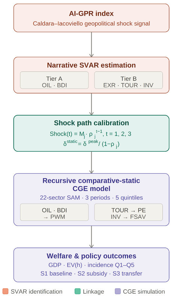
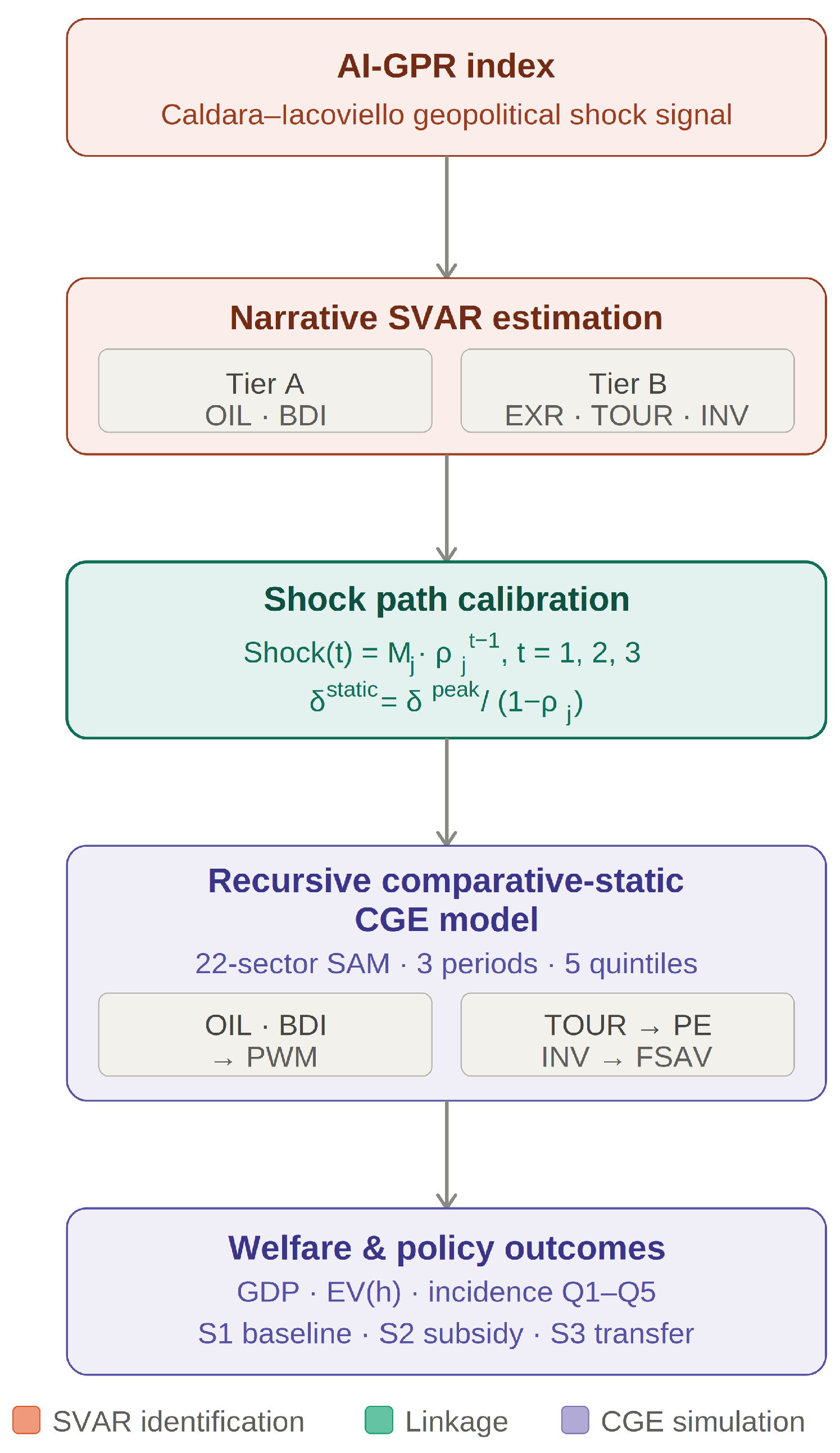
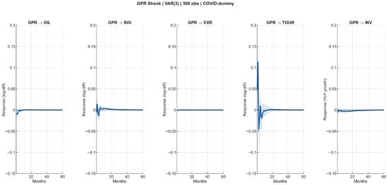
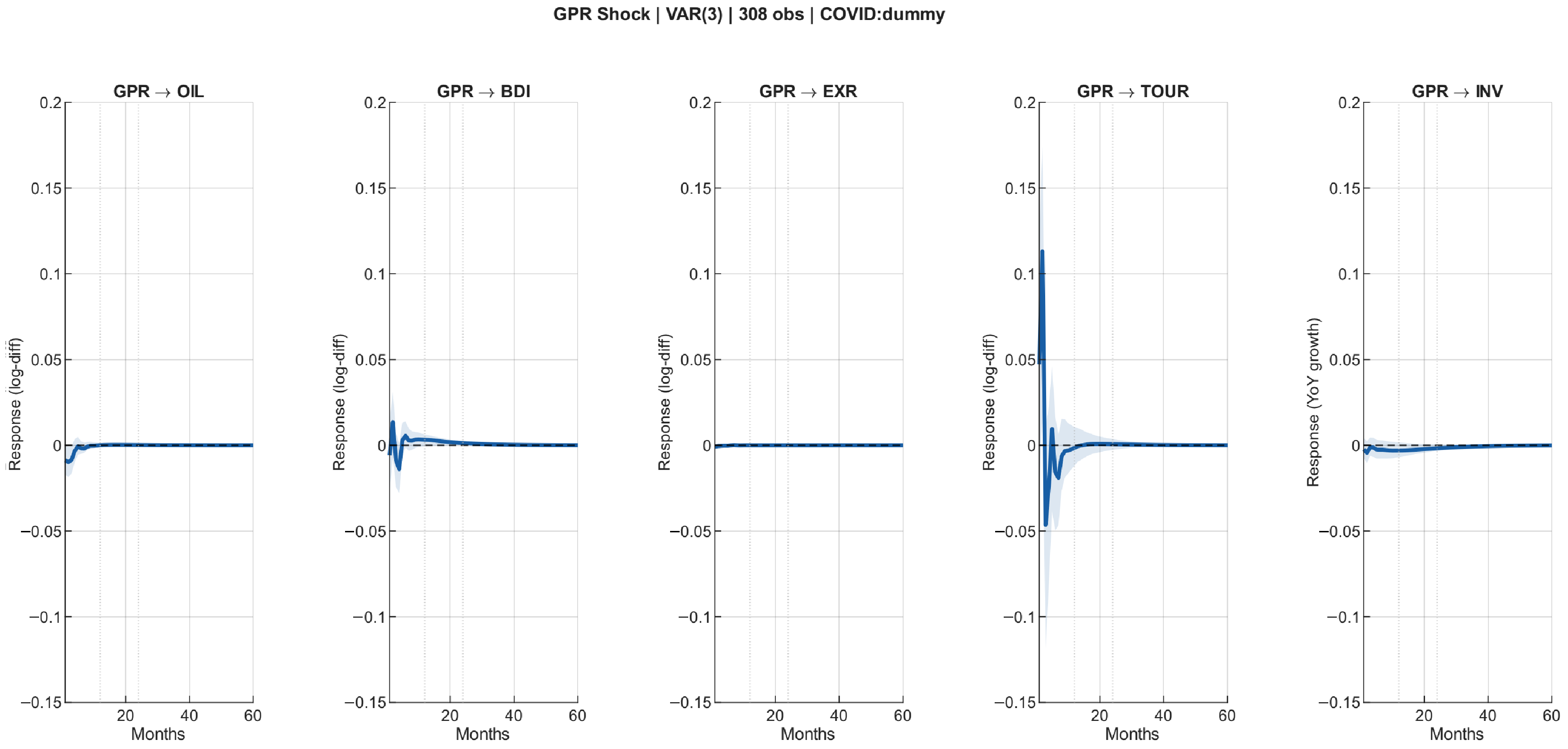
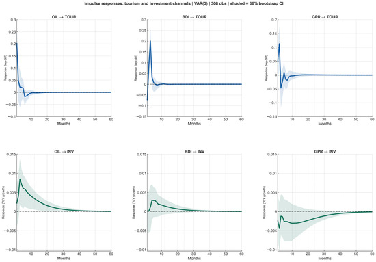
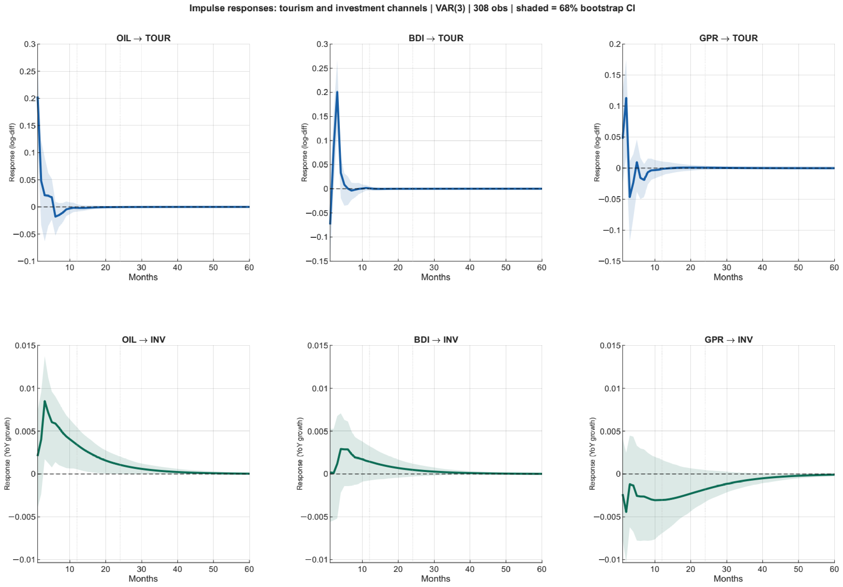
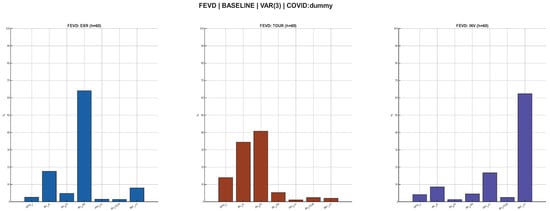
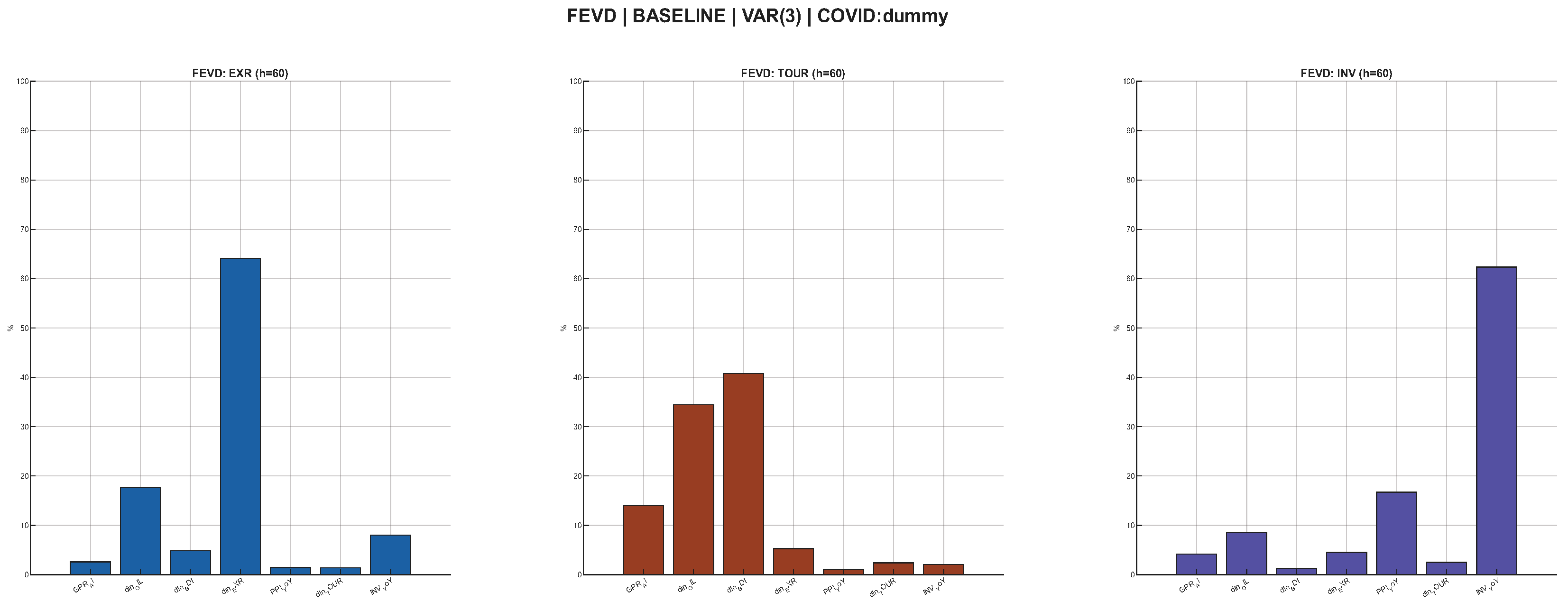

Disclaimer/Publisher’s Note: The statements, opinions and data contained in all publications are solely those of the individual author(s) and contributor(s) and not of MDPI and/or the editor(s). MDPI and/or the editor(s) disclaim responsibility for any injury to people or property resulting from any ideas, methods, instructions or products referred to in the content. |
© 2026 by the author. Licensee MDPI, Basel, Switzerland. This article is an open access article distributed under the terms and conditions of the Creative Commons Attribution (CC BY) license.