


Abstract
Peruvian fresh-grape exports have expanded substantially but remain concentrated in a limited number of markets. This study examines the factors associated with bilateral export value for 17 destinations during 2001–2024, using a balanced panel of 408 observations, including 80 zero-export observations (19.61%). An augmented gravity model is estimated by Poisson pseudo-maximum likelihood (PPML) with destination and year fixed effects; linear models serve as comparisons. Destination-country gross domestic product (GDP) has a positive coefficient of 1.4118, but its inferential evidence varies across the conventional clustered normal test (p = 0.0424), restricted score test (p = 0.0869), and cluster jackknife (p = 0.5095). The population estimate is exceptionally large and specification-sensitive; distance and the common oil price are not separately identified under the fixed effects employed. Across the 17 destinations, the Herfindahl–Hirschman concentration index increased from 0.2858 to 0.3162 between 2001 and 2024, while destinations with no initial exports accounted for 31.55% of the increase in export value. This study contributes product-specific evidence on zero flows, market concentration, and inferential sensitivity without establishing causal effects or generalizing to excluded markets.
1. Introduction
Peruvian fresh-grape exports reached USD 1.7052 billion in 2024 and were shipped to 48 destination markets, reflecting the growing relevance of the product within Peru’s agricultural export portfolio and its participation in international fresh-food supply chains (International Trade Centre, 2024). This expansion has taken place within a broader transformation of Latin American agri-food trade, characterized by sustained export growth and increasing participation in global agricultural markets over recent decades (Ayuda et al., 2024, 2026). Nevertheless, this growth coexists with substantial geographical concentration. In 2024, the United States, the Netherlands, and Mexico jointly accounted for approximately 72.7% of Peru’s total fresh-grape export value, while the 17 destinations included in this study represented 93.7% of the national total, according to the authors’ calculations based on International Trade Centre data (International Trade Centre data, 2024). This structure makes export performance particularly dependent on the economic and commercial conditions prevailing in a relatively limited number of destination markets.
Fresh-fruit trade is subject to specific conditions that make aggregate export growth alone insufficient to explain bilateral performance. Agricultural products face particular market-entry requirements, while perishability increases the importance of transit time, logistics coordination, regulatory conditions, and continuity of market access (Serrano & Pinilla, 2012). Evidence across different fruit markets suggests that economic size, distance, prices, exchange rates, competition, trade protection, and market-access conditions may be associated with export flows in different ways depending on the product and destination considered (Alves et al., 2014; Lubinga et al., 2026; Nunes et al., 2021; Rangkakulnuwat, 2024). Geographical distance alone also provides only a partial representation of effective trade costs, as maritime connectivity, port efficiency, and logistics performance can alter the conditions under which perishable products reach importing markets (Del Rosal, 2024; Sant’Anna & Kannebley Junior, 2018; Zaninović et al., 2021). Regulatory requirements add another dimension, with their trade implications varying according to the type of measure, regulatory homogeneity, and exporters’ capacity to comply with traceability and technical adaptation requirements (Bispo et al., 2025; Fiankor & Shingal, 2025; Karagulle et al., 2026).
In this context, the gravity model provides an appropriate analytical framework for examining bilateral trade flows because it relates trade to market size and trade frictions and can be augmented to incorporate demographic, macroeconomic, regulatory, and trade-policy conditions (Metin & Tepe, 2021; Tuñoque-Morante et al., 2025). However, gravity-model estimates may be sensitive to unobserved heterogeneity across trading partners, heteroskedasticity, zero trade flows, and estimator choice, making it necessary to evaluate the robustness of the identified relationships across alternative specifications (Gómez-Herrera, 2013). Exchange-rate conditions constitute an additional dimension of the trading environment because they may modify external competitiveness and uncertainty in international trade flows (Silva et al., 2016). Accordingly, analysis of fresh-grape exports requires simultaneous consideration of demand conditions, trade frictions, and macroeconomic and regulatory factors rather than attributing bilateral performance to a single determinant.
Despite the increasing use of gravity models in agricultural and fresh-fruit trade, the literature reviewed for this study did not identify an equivalent long-period bilateral analysis of Peruvian fresh-grape exports to their principal destination markets that jointly examines destination-market economic and demographic size, geographical distance, international oil prices, tariffs, technical barriers to trade (TBTs), the real effective exchange rate, and trade agreements. Evidence is also limited regarding whether the estimated relationships for this particular product remain stable under alternative treatments of partner heterogeneity, heteroskedasticity, and zero trade flows. This gap is relevant because findings obtained for other agricultural products or exporting countries may not be directly generalizable to the structure of Peruvian fresh-grape trade.
This study’s relevance lies in distinguishing potential demand size from the specific trading conditions of a perishable product. Its scope is restricted to 17 markets selected among the principal destinations in 2024, conditional on availability of complete annual series for 2001–2024. Although these destinations represented approximately 93.7% of Peru’s total fresh-grape export value in that year, selection based on commercial importance and statistical coverage precludes extrapolation to all potential importers or identification of market-entry determinants for excluded countries. The study estimates associations within the observed panel, not causal effects or forecasts for destinations outside the sample.
The study makes three complementary contributions. First, it reassesses augmented-gravity relationships using PPML in levels with destination and year fixed effects, retaining 80 zero flows and treating historical linear estimates only as comparisons. Second, it evaluates the fragility of conventional inference with 17 clusters and coefficient sensitivity to particular destinations and alternative procedures. Third, it documents trade concentration and transitions from zero to positive flows within those same markets, without treating these transitions as an identified structural extensive margin or attributing them to trade agreements. The contributions distinguish estimated associations, information limitations, and descriptive evidence relevant to market evaluation; they do not establish the causal effects of policies.
Accordingly, the objective is to analyze the economic, demographic, geographic, macroeconomic, regulatory, and trade-policy factors associated with bilateral fresh-grape export value from Peru to 17 principal destinations during 2001–2024. The research question is as follows: Which factors are associated with the bilateral trade flow of Peruvian fresh-grape exports over this period?
The analysis supplies long-term evidence for a major agricultural export product and examines the stability of the relationships through PPML in levels, comparative linear models, and sensitivity tests that retain zero flows. Its applied scope concerns market assessment, diversification, and market-access conditions, without inferring causal effects of individual decisions.
2. Literature Review
2.1. Empirical Foundations
Empirical applications of the gravity model to fresh-fruit trade indicate that economic size, geographical frictions, regulatory conditions, and market-access factors do not affect all products and destinations uniformly. The closest empirical precedent to the present study is Alves et al. (2014), who examined Brazilian grape exports during 1995–2009. Their estimates showed positive and statistically significant relationships for Brazilian GDP and sanitary and phytosanitary (SPS) measures, whereas distance, tariffs, and technical barriers to trade (TBTs) did not display statistically significant effects in the reported specification. Evidence for Brazilian papaya similarly associated economic size with higher exports and geographical distance with lower trade, while exchange rates and international prices exhibited direct relationships (Nunes et al., 2021). Studies of Thai mangosteen and durian and South African avocados further indicate that export potential varies across destinations according to complementarity, competition, protection, and market-access conditions (Lubinga et al., 2026; Rangkakulnuwat, 2024). Collectively, these findings suggest that the determinants observed for one fresh-fruit sector may not be directly generalizable to Peruvian fresh-grape trade.
Broader agricultural-gravity evidence identifies economic size as one of the most recurrent determinants of bilateral trade, although the magnitude and significance of other variables vary across products and empirical specifications. Balogh and Borges Aguiar (2022), using a large panel of Latin American and Caribbean agricultural trade flows, found positive relationships for exporter and importer GDP and a negative relationship for geographical distance. Agricultural applications have also incorporated population, production, exchange rates, tariffs, institutional factors, language, borders, and trade agreements through fixed-effects, random-effects, dynamic-panel, PPML, Heckman-type, and related gravity specifications (Balogh & Leitão, 2019; Braha et al., 2017; Kondaridze & Luckstead, 2023; Ravi Kumar et al., 2024; Szerb et al., 2022). However, trade openness and related policy variables do not exhibit uniform relationships across countries and agricultural products (Matkovski et al., 2017). The available evidence therefore points to a relatively persistent role for economic size, while the contribution of demographic, geographical, productive, and policy variables appears more dependent on the characteristics of the product, market, and model specification.
Trade agreements provide a particularly heterogeneous source of variation in agricultural trade. Mujahid and Kalkuhl (2016) showed that agreements may increase food trade, redirect it across markets, or generate effects that emerge only after several periods. At the Latin American level, international demand and regional integration contributed substantially to the agricultural export expansion documented by Ayuda et al. (2024), but the contribution of individual determinants varied across products and destinations. Ayuda et al. (2026) subsequently showed that the effects of regional trade agreements differ according to agreement type, destination region, and period. Similar heterogeneity appears in evidence on agricultural trade associated with the Belt and Road Initiative, where outcomes varied with participating countries’ income levels (Zhao et al., 2024), and in global wine trade, where language, culture, and agreements were jointly related to bilateral flows (Balogh & Jámbor, 2018). Structural-gravity evidence for MERCOSUR also emphasizes the importance of distinguishing among specific integration arrangements rather than treating trade agreements as homogeneous interventions (Da Silva & Silva, 2024). Institutional quality and institutional distance provide an additional source of heterogeneity in export performance (Abreo et al., 2021), while external shocks can alter supply- and demand-side trade conditions, as illustrated by the differentiated effects identified during the COVID-19 pandemic (Ridley et al., 2023). Consequently, the formal existence of a trade agreement does not by itself imply a uniform increase in agricultural exports.
Regulatory measures exhibit even greater empirical ambiguity. The broader literature on non-tariff measures indicates that their effects may differ according to the trade margin examined, exporter persistence, regulatory compatibility, and firms’ capacity to comply. Karagulle et al. (2026) distinguished between effects on agricultural export intensity and exporter persistence, whereas Fiankor and Shingal (2025) showed that the degree of regulatory homogeneity can influence firms’ import decisions. Traceability requirements may also reshape agri-food trade by verifying product origin and processing and by affecting buyer confidence (Bispo et al., 2025). Importantly, SPS measures and TBTs should not be treated as interchangeable restrictions, because their economic mechanisms and empirical effects may differ (Gouveia et al., 2026). Evidence regarding port wine likewise demonstrates the relevance of considering non-tariff measures jointly with macroeconomic and climatic conditions rather than assuming an isolated regulatory effect (Macedo et al., 2020a). The Brazilian grape study reinforces this distinction; SPS measures showed a positive and statistically significant relationship with exports, whereas TBTs did not show statistically significant evidence (Alves et al., 2014). Thus, regulatory requirements may restrict trade, have no detectable association, or facilitate market access under particular conditions. Accordingly, the present study treats TBTs as a specific observed regulatory dimension rather than assuming that all non-tariff measures constitute equivalent barriers.
Trade costs also extend beyond geographical distance. For perishable agricultural products, the effective burden of supplying a foreign market can depend on port efficiency, maritime connectivity, transit conditions, and logistics performance. Sant’Anna and Kannebley Junior (2018) found that port delays had quantifiable consequences for Brazilian exports, with each additional hour of relative dwell time associated with an approximately 2% reduction in relative exports. Evidence from trade between the EU15 and Central and Eastern European countries similarly showed that the relationship between logistics performance and bilateral trade differed across product classes and country groups (Zaninović et al., 2021). Subsequent research linked international logistics and institutional conditions to participation in global value-chain trade (Zaninović & Bugarčić, 2023). These findings indicate that geographical distance is only a partial proxy for effective trade frictions. Countries separated by similar physical distances may face different commercial conditions because of variations in connectivity, infrastructure, port operations, and logistics performance. This distinction is particularly relevant when examining fresh-fruit exports, for which delays and coordination failures may be economically consequential.
Methodological evidence further shows that estimated gravity relationships can be sensitive to the choice of econometric specification. Gómez-Herrera (2013) compared alternative gravity estimators and concluded that no single method dominates across all datasets; estimator performance depends on characteristics such as zero trade flows, heteroskedasticity, unobserved heterogeneity, and non-random selection. More recent methodological developments reinforce the need to distinguish between alternative treatments of these problems. Structural-gravity approaches incorporate broader equilibrium restrictions and multilateral trade relationships (Heid et al., 2021; Pfaffermayr, 2020), while nonlinear estimators do not automatically resolve every specification or selection problem associated with zero bilateral flows (Mnasri & Nechi, 2021). Bilateral relationships may also vary over time, making time-varying heterogeneity relevant to gravity estimation (Baier & Standaert, 2024). Similarly, pooled specifications may conceal systematic differences across partners and periods (Ghaddab, 2026). This issue is especially relevant for sparse agricultural trade matrices; Caravaggio and Conigliani (2026), for example, analyzed Latin American timber trade in a dataset in which 81% of bilateral flows were zero. Taken together, these studies support evaluating whether substantive conclusions remain stable across panel and nonlinear specifications rather than relying exclusively on a single estimator.
Overall, the reviewed literature establishes economic size as a recurrent correlate of agricultural bilateral trade but provides substantially less uniform evidence for population, geographical distance, trade agreements, tariffs, regulatory measures, logistics conditions, and other market-specific factors. The direction, magnitude, and statistical significance of these relationships frequently vary according to the agricultural product, destination market, regulatory environment, sample composition, and econometric specification. Existing applications cover Brazilian grapes and papaya, Thai mangosteen and durian, South African avocados, wine, rice, maize, dairy products, timber, and broader agricultural trade, thereby providing a substantial empirical basis for gravity-model applications. Nevertheless, within the literature reviewed for this study, no equivalent long-period bilateral analysis was identified for Peruvian fresh-grape exports that jointly evaluates destination-market characteristics, geographical and trade-cost variables, tariff and regulatory conditions, trade agreements, and the sensitivity of the estimated relationships to zero trade flows and alternative econometric specifications. This unresolved empirical gap motivates the application of an augmented gravity framework to Peru’s principal fresh-grape export destinations during 2001–2024.
2.2. Theoretical Framework
2.2.1. The Gravity Model in International Trade
The gravity model provides a widely used framework for examining bilateral trade flows. Its basic logic establishes that trade between two economies is positively related to their economic size and negatively related to the frictions that impede exchange. From this perspective, economic conditions in the exporting country represent its potential supply capacity, whereas the economic size of the importing country approximates its demand and absorption capacity. Bilateral distance, in turn, represents frictions associated with transportation, time, coordination, and information costs (Tinbergen, 1962; Metin & Tepe, 2021; Tuñoque-Morante et al., 2025).
Subsequent theoretical developments broadened this formulation by recognizing that bilateral trade costs cannot be evaluated independently of the alternative trading opportunities available to each economy. The introduction of multilateral resistance terms implies that trade between two countries depends not only on their bilateral costs but also on the relative costs of trading with alternative partners (Anderson & van Wincoop, 2003). Spatial approaches further emphasize that geographical location and economic relationships may generate interactions extending beyond a single bilateral-distance measure (LeSage & Pace, 2009). These developments provide the conceptual foundation for the present analysis; however, this study employs an augmented empirical gravity model rather than a complete structural-gravity specification.
Empirical gravity estimation also raises econometric considerations. Bilateral relationships repeatedly observed over time may contain unobserved partner heterogeneity, while heteroskedasticity and zero trade flows can affect conventional log-linear specifications (Cameron & Trivedi, 2005; Gujarati & Porter, 2010; Wooldridge, 2010). In this context, multiplicative specifications estimated through PPML provide an alternative that can retain zero-valued trade observations. Nevertheless, no estimation strategy automatically resolves all problems arising from selection, heterogeneity, or model misspecification (Gómez-Herrera, 2013; Mnasri & Nechi, 2021; Pfaffermayr, 2020). The specific estimator-selection and diagnostic procedures are therefore addressed in the methodology.
With a single exporter observed over time, destination fixed effects control for time-invariant partner characteristics, whereas year effects capture shared shocks. This imposes identification restrictions; fixed bilateral distance cannot be estimated separately from destination effects, and Peru’s GDP and population, as well as the common WTI oil price, are captured by year effects. These restrictions do not negate the underlying economic mechanisms; rather, they delimit the slopes identified by the principal model (Anderson & van Wincoop, 2003; Head & Mayer, 2014; Santos Silva & Tenreyro, 2006).
2.2.2. Economic Size and Market Demand
Partner-country GDP represents a central demand-side mechanism within the gravity framework. A larger importing economy may possess greater purchasing capacity, broader aggregate demand, and a stronger ability to absorb imported goods. Evidence from agricultural and fresh-fruit trade consistently highlights the relevance of economic size, although the magnitude of its relationship with trade varies across products and specifications (Alves et al., 2014; Balogh & Borges Aguiar, 2022; Nunes et al., 2021). Accordingly, partner-country GDP is expected to be positively associated with the bilateral value of Peruvian fresh-grape exports.
Partner-country population captures a complementary dimension of potential market size. A larger population may expand the consumer base and increase aggregate demand for imported food products. However, its relationship with trade may depend on income, domestic production, consumption patterns, and the information it shares with other measures of market size. Agricultural applications have considered GDP and population jointly as distinct dimensions of destination-market capacity (Ravi Kumar et al., 2024). A positive relationship is therefore maintained for partner population, although its independent contribution may differ from that of GDP.
Exporter-side conditions also form part of the gravity framework. Peru’s GDP may proxy the scale of the exporting economy and its general capacity to sustain supply to foreign markets. Peru’s population has a less unambiguous interpretation because a larger population may be associated with productive resources while simultaneously increasing domestic absorption. Agricultural applications have incorporated exporter-side macroeconomic and productive characteristics to represent supply conditions (Caravaggio & Conigliani, 2026; Kondaridze & Luckstead, 2023; Macedo et al., 2020b). In the present specification, Peru GDP and Peru population operate as exporter-side controls. Although agricultural production variables have been included in previous studies, Peruvian grape production is not part of the final estimated model.
2.2.3. Trade Costs and Macroeconomic Conditions
Bilateral distance represents a structural trade friction. Greater separation between exporter and importer may increase transportation, time, coordination, and information costs and thereby reduce the intensity of bilateral exchange. This negative relationship is recurrent in gravity applications to agricultural and fresh-fruit trade (Balogh & Borges Aguiar, 2022; Nunes et al., 2021; Szerb et al., 2022). For a perishable product such as fresh grapes, these frictions may be particularly relevant because appropriate logistics conditions must be maintained throughout transportation.
Geographical distance, however, does not constitute a complete measure of effective logistics costs. Markets located at similar physical distances may differ substantially in maritime connectivity, route availability, service frequency, infrastructure, and port efficiency (Del Rosal, 2024; Sant’Anna & Kannebley Junior, 2018). Bilateral distance should therefore be interpreted as a structural proxy for trade frictions rather than as an exhaustive representation of the logistics conditions faced by fresh-grape exports.
The international WTI oil price introduces an additional macroeconomic channel. Higher oil prices may increase fuel, transportation, refrigeration, energy, and input costs associated with the production and international distribution of perishable products. This cost channel could generate a negative relationship with trade. However, oil prices may also move jointly with global economic activity, commodity-price cycles, and international demand. Previous evidence consequently reports negative, positive, asymmetric, and statistically non-significant responses across products, markets, and periods (Baek & Choi, 2020; Hu & Puah, 2025; Jain et al., 2025; Vatsa & Baek, 2024). Accordingly, the expected relationship between WTI and bilateral trade is theoretically treated as non-directional.
2.2.4. Trade Policy and Regulatory Conditions
Tariffs represent a direct trade friction because they increase the entry price of imported goods. Higher tariff rates may reduce the relative competitiveness of Peruvian grapes compared with alternative suppliers or substitute products and, through this mechanism, reduce import demand. Their observed effect may nevertheless depend on competition, market demand, effective preference utilization, and interactions with other market-access requirements (Alves et al., 2014; Kondaridze & Luckstead, 2023; Matkovski et al., 2017; Mujahid & Kalkuhl, 2016). A negative expected relationship between tariffs and bilateral trade is therefore maintained.
Non-tariff measures constitute a broad regulatory category within which sanitary and phytosanitary measures (SPS) and technical barriers to trade (TBTs) represent conceptually distinct instruments. This distinction is particularly important because the empirical variable incorporated into the present model specifically measures the number of technical barriers to trade (TBTs) rather than an aggregate measure of all NTM or SPS requirements.
TBTs may increase technical-adjustment, certification, documentation, and compliance costs, thereby raising market-entry costs. This restrictive channel provides a theoretical basis for expecting a negative relationship between TBTs and bilateral trade. Nevertheless, certain technical requirements may also reduce information asymmetries, improve regulatory compatibility, strengthen traceability, and signal product quality or safety to international buyers. Their observed trade implications may therefore vary according to the type and degree of regulatory harmonization and exporters’ capacity to comply (Alves et al., 2014; Bispo et al., 2025; Fiankor & Shingal, 2025; Gouveia et al., 2026). The existence of this alternative mechanism indicates that the empirical effect of TBTs may depend on the specific characteristics of the regulation and market under consideration.
Trade agreements may reduce bilateral frictions through tariff reductions, preferential access, lower information costs, and greater predictability of trade relations. Nevertheless, the formal existence of an agreement does not necessarily imply full preference utilization or homogeneous effects across products and destination markets. Agreement depth, effective utilization of preferences, destination-market characteristics, and time since entry into force may condition their trade effects (Ayuda et al., 2024, 2026; Balogh & Borges Aguiar, 2022; Mujahid & Kalkuhl, 2016). Despite this heterogeneity, the predominant theoretical mechanism supports an expected positive association between trade agreements and bilateral exports.
2.2.5. Exchange-Rate Conditions
The real effective exchange rate (REER) represents an economy’s relative-price conditions against its trading partners after accounting for price differentials. Its relationship with trade depends on both the construction of the index and the economic interpretation of its movements. In general, changes in the REER may alter relative competitiveness and the conditions under which exporters and importers conduct international transactions.
The level of the REER should also be distinguished from exchange-rate volatility. Volatility may increase uncertainty regarding prices, contracts, and trade revenues, whereas the REER level primarily operates through relative prices. The literature has incorporated both dimensions and shows that their relationships with trade vary across countries, products, trade structures, and estimation methods (Abdullah et al., 2024; Benlaria, 2024; F. Chen et al., 2023; Coşkuner & Sogah, 2023; Silva et al., 2016; Vo et al., 2024). Agricultural and Latin American applications likewise support considering exchange-rate conditions jointly with other gravity variables (Caravaggio & Conigliani, 2026; Macedo et al., 2020b).
From a conceptual perspective, a negative relationship may be expected when changes in the REER deteriorate relative competitiveness or increase the effective cost of trade from the perspective relevant to the bilateral flow being analyzed. However, the precise economic interpretation of this direction depends on the specific construction of the REER index and on the meaning assigned to increases or decreases in that indicator. Accordingly, this interpretation should remain linked to the definition of the variable used in the database rather than being inferred from the subsequent econometric results.
2.2.6. Conceptual Model and Research Hypotheses
The dependent variable is the bilateral FOB value of Peruvian fresh-grape exports. The conceptual model incorporates Peru GDP, partner-country GDP, Peru population, partner-country population, bilateral distance, the international WTI oil price, tariffs, technical barriers to trade, the real effective exchange rate, and trade agreements.
The proposed functional relationship is:
where i denotes the destination country and t denotes the year. The expression represents the proposed determinants conceptually and is distinct from the econometric specification subsequently estimated as it.
Based on the theoretical mechanisms developed above, the following hypotheses are proposed:
H1.
Partner-country GDP is positively associated with the bilateral flow of Peruvian fresh-grape exports;
H2.
Partner-country population is positively associated with the bilateral flow of Peruvian fresh-grape exports;
H3.
Bilateral distance is negatively associated with the bilateral flow of Peruvian fresh-grape exports;
H4.
The international WTI oil price is significantly associated with the bilateral flow of Peruvian fresh-grape exports;
H5.
Tariffs are negatively associated with the bilateral flow of Peruvian fresh-grape exports;
H6.
Technical barriers to trade (TBTs) are negatively associated with the bilateral flow of Peruvian fresh-grape exports;
H7.
The real effective exchange rate (REER) is negatively associated with the bilateral flow of Peruvian fresh-grape exports.
H8.
Trade agreements are positively associated with the bilateral flow of Peruvian fresh-grape exports.
The eight hypotheses represent ex ante expectations and are not reformulated to match estimated coefficients. Their empirical assessment distinguishes statistical uncertainty from non-identification under fixed effects. Distance (H3) and WTI (H4) remain theoretically relevant even though their slopes cannot be separately identified in the primary PPML specification. Inference is limited to the 17 destinations and does not demonstrate causality.
2.2.7. Empirical Evidence Supporting the Hypotheses
Table 1 synthesizes quantitative evidence relevant to formulating hypotheses H1–H8 before estimation. It presents coefficients, elasticities, significance levels, and percentage effects reported in published studies on variables of the augmented gravity model. The synthesis does not assume universal relationships or anticipate this study’s results; instead, it supplies empirical grounds for the expected signs while recognizing differences in magnitude, statistical significance, and direction across products, markets, and specifications.
Table 1.
Quantitative empirical evidence supporting research hypotheses.
The estimates in Table 1 come from studies with different products, samples, scales, and measures. Parameters from log-linear, PPML, and selection models must not be treated as directly comparable elasticities. In particular, evidence based on an exporter’s REER does not directly identify the association of the importer’s REER used in this study. Thus, the table informs ex ante hypotheses but does not establish them for Peruvian grapes.
Figure 1 summarizes the theoretical expectations: H1, H2, and H8 have positive expected signs; H3, H5, H6, and H7 have negative signs; and H4 has no predetermined direction because distinct mechanisms link oil prices to agricultural trade. These expectations precede estimation and do not anticipate the empirical findings.
Figure 1.
Conceptual model of the determinants of bilateral Peruvian fresh-grape export flows. Note. The signs (+/−) indicate the directions expected under hypotheses H1–H8 of the augmented gravity model.
3. Methodology
3.1. Research Approach, Design, and Scope
This study employed a quantitative approach, an explanatory scope understood as the analysis of statistical associations, and a non-experimental, longitudinal, retrospective design based on secondary information. Economic, demographic, commercial, geographical, regulatory, and exchange-rate conditions were not manipulated. Thus, the parameters describe associations conditional on the specification and included destinations, rather than causal effects. The research design draws on relevant methodological foundations (Ajimotokan, 2023; Creswell & Creswell, 2022; Edmonds & Kennedy, 2017; Pacheco & Cruz, 2006; Quispe Berríos et al., 2023; Watson, 2015; Hernández-Sampieri & Mendoza, 2023).
An augmented gravity model was applied to the annual free-on-board (FOB) value of Peruvian fresh-grape exports classified under Harmonized System subheading HS 080610. The unit of analysis was the destination country-year, with Peru as the sole exporter. The study covered 24 consecutive years, 2001–2024. The consolidated balanced panel contains 17 destinations and 408 observations (17 × 24), with no duplicate destination-year combinations or missing values within the final sample. All 80 zero-export observations (19.61%) were retained without replacing them with artificial positive flows, an important consideration for estimator selection (LeSage & Pace, 2009; Vo et al., 2024).
Market selection began with the principal destinations of Peruvian fresh grapes identified in ITC Trade Map for 2024, the last reference year for which the required annual information was available. A longitudinal-coverage criterion was then applied; destinations were retained only when the necessary set of variables could be assembled for 2001–2024. Other candidate countries were excluded because at least one series was incomplete and the gaps could not be satisfactorily addressed using alternative sources or adequately justified imputation procedures during compilation. This analytic-sample rule does not constitute random sampling or evidence of absent trade with excluded countries. The 17 destinations were Canada, China, Colombia, Costa Rica, the Dominican Republic, Hong Kong, Italy, Japan, Mexico, the Netherlands, Norway, Russia, South Korea, Spain, the United Kingdom, the United States, and Venezuela. Together, these accounted for approximately 93.7% of national export value for the product in 2024. Selection by trade importance and data completeness constrains representativeness and may generate selection bias relative to all potential destinations. Accordingly, inference concerns these 17 countries and cannot be generalized to smaller or excluded markets. The year 2025 was omitted because equivalent consolidated annual coverage was unavailable for all variables.
3.2. Data Sources, Variable Operationalization, and Treatment
Records were assembled by documentary analysis and matched by trading partner and year, consistently using product subheading HS 080610. Export value was determined according to the ITC Trade Map; nominal GDP and total population for Peru and its partners from the World Bank’s World Development Indicators (WDIs); reference maritime distance from MarineTraffic; the international WTI crude-oil price from the U.S. Energy Information Administration (EIA); tariffs from the ITC Market Access Map; technical barriers to trade (TBTs) from the World Trade Organization (WTO) platform; trade agreements from MINCETUR; and the real effective exchange rate (REER) from World Bank indicator PX.REX.REER, based on International Monetary Fund (IMF) statistics. A unique destination-year identifier was used in compiling and reviewing the consolidated records (Hernández-Sampieri & Mendoza, 2023; Arias Gonzáles, 2020).
Table 2 reports each variable’s operational scope, source, observable indicator, unit, and econometric treatment. The original nominal magnitudes were preserved in the dataset. Export value is expressed in USD millions only when fitting PPML, whereas the historical transformation of FOB value expressed in USD is retained for the linear comparisons. Variable definitions are independent of the signs or statistical significance of the resulting coefficients.
Table 2.
Variables, indicators, units, transformations, and data sources.
The FOB measure (Y) records the value of Peru’s fresh-grape exports (HS 080610) to each partner each year in current USD, without separating quantities, prices, or grape varieties. Peru’s GDP and partner GDP were recorded in current USD as measures of economic size; their populations represent annual inhabitants in persons. Peru’s GDP and population have common values across the 17 destinations each year, while importer measures vary across countries and time. WTI is the EIA’s international annual crude-oil benchmark in USD per barrel, also common to all destinations within a year. These measures capture economic scale, demographics, and energy conditions in the gravity framework but do not directly measure grape production, product-specific demand, or logistics expenditure.
Technical barriers to trade (TBTs) were operationalized as the annual count of technical measures registered on the WTO platform for HS 080610. The query combined the relevant importing or notifying country, Peru as the exporting country considered, and the fresh-grape product classification. The destination-year series records technical-measure incidence associated with this subheading, not all non-tariff measures applicable to other products or sectors. The count does not measure regulatory restrictiveness, severity, harmonization, certification expenditure, or actual compliance costs; neither is it equivalent to sanitary and phytosanitary (SPS) measures. The transformation ln(1 + TBT) retains zero counts.
The tariff variable (TA) was constructed from percentage rates reported by the ITC Market Access Map for imports of Peruvian-origin HS 080610 by each destination and year. The lowest available percentage was recorded from the most-favored-nation (MFN) and corresponding preferential rate when a preference was reported. Thus, TA is the lowest nominal reference duty available under the regimes considered, expressed in percentage points, rather than necessarily the MFN tariff or the tariff actually paid. Claiming a preference may require documented origin and other conditions; selecting the minimum does not demonstrate its actual utilization. ln(1 + TA) was employed to retain zero rates.
Bilateral maritime distance (D) was obtained from MarineTraffic in nautical miles between selected principal or representative seaport pairs for Peru and each trading partner. One value per Peru–destination pair was held constant over 2001–2024 to approximate geographical separation in the gravity model. The ports serve as geographic reference points; their selection does not imply that all grape shipments followed that route. The measure is not intended to evaluate or optimize actual logistics routes and does not capture shipping-service frequency, connectivity, transshipment, freight rates, transit times, or cold-chain performance. ln(D) was used in specifications where distance could be separately identified.
The trade-agreement indicator (FTA) was coded as binary using MINCETUR institutional records. It includes bilateral and multilateral treaties and commercial-integration arrangements involving Peru and the destination country. A value of 1 was assigned whenever at least one agreement was in force during the calendar year, beginning with its official entry-into-force year and continuing while effective; 0 was assigned for years without an agreement in force. This definition does not distinguish the number of concurrent agreements or measure agreement depth, provisions specific to HS 080610, preference margins, actual preference use, compliance with rules of origin, or realized tariff reductions. The original 0/1 scale was retained without logarithmic transformation.
The REER is the annual multilateral index of each importing country, not Peru’s REER and not a bilateral quotation against the Peruvian Sol. The source was the World Bank WDI indicator PX.REX.REER, constructed from IMF International Financial Statistics with a 2010 = 100 base. This tracks the nominal effective exchange rate against a trade-weighted currency basket adjusted for relative prices or costs; it does not directly quantify exchange-rate volatility. The gravity specifications use ln(REER), retaining the international series’ definition and direction.
Fourteen missing REER observations were filled using univariate forecasts fitted exclusively on series available before each forecast horizon. For Venezuela, ln(REER) for 2001–2016 was modeled using Holt exponential smoothing with an additive damped trend; forecasts for 2017–2024 were exponentiated back to index levels. For Hong Kong, an ARIMA(1, 0, 0) model with a constant was fitted to the index levels for 2001–2021 and projected over 2022–2024. For South Korea, ARIMA(1, 1, 1) without drift was fitted to ln(REER) for 2001–2021 and projected over 2022–2024, followed by exponentiation. No observations after the last available estimation year were used in fitting the forecasts.
Computational replication in Python 3.15.2 using statsmodels documented the three forecast specifications and parameters. For Venezuela, the damped-trend coefficient was 0.9446549 and the level and trend smoothing coefficients were approximately 0.9752689. For Hong Kong, ARIMA(1, 0, 0) yielded a constant of 129.9781039 and an autoregressive parameter of 0.9352114. For South Korea, ARIMA(1, 1, 1) yielded AR(1) = −0.3293329 and MA(1) = 0.9923260. Sensitivity exercises described below assess the influence of these completed series; the extreme magnitudes are reported in the Results rather than represented as direct official observations for forecast years.
Natural logarithms were taken for strictly positive measures (GDP, population, distance, WTI, and REER). For tariffs and TBT counts, which can be zero, ln(1 + x) was used; FTA remained binary. The dependent variable was retained in levels—USD divided by one million for numerical convenience—in the PPML models. Historical linear models use ln(1 + Y) with Y in USD; their coefficients are not conventional export elasticities because the added constant changes interpretation and the result depends on the monetary unit. Likewise, the ln(1 + x) transformation of tariffs and TBTs did not generate a constant elasticity with respect to the original x at all values (Eichengreen & Irwin, 1998; Burger et al., 2009; Philippidis et al., 2013; Jafta & Phali, 2025).
3.3. Econometric Specification and Identification
The primary estimation strategy applied Poisson pseudo-maximum likelihood (PPML) to FOB export value in levels, specifying a multiplicative conditional mean. It retains zero trade flows and does not require the dependent variable itself to follow a Poisson distribution when the conditional mean is correctly specified. Three incrementally specified models were compared: M1, basic PPML without fixed effects; M2, PPML with destination fixed effects; and M3, PPML with destination and year fixed effects. M3 was designated as the principal specification to control time-invariant destination characteristics and shared time shocks, without claiming to estimate a complete global structural-gravity equilibrium or all multilateral resistance terms (Anderson & van Wincoop, 2003; Head & Mayer, 2014; Santos Silva & Tenreyro, 2006).
E(Yit/106|Xit, αi, λt) = exp[αi + λt + β1 ln(GDP_partnerit) + β2 ln(POP_partnerit)
+ β3 ln(1 + TAit) + β4 ln(1 + TBTit) + β5 FTAit + β6 ln(REERit)]
+ β3 ln(1 + TAit) + β4 ln(1 + TBTit) + β5 FTAit + β6 ln(REERit)]
In Equation (2), i indexes destination and t indexes year; αi captures destination heterogeneity and λt represents year fixed effects. The conditional mean is expressed in USD millions for numerical stability. Uniform rescaling changes the intercept or fixed-effect component but not the slope coefficients. A regressor specified as ln(x) has a coefficient interpretable as the elasticity of conditional expected FOB with respect to x under model assumptions. For ln(1 + x), the coefficient is an elasticity with respect to 1 + x, not necessarily x. For the binary FTA indicator, the conditional percentage difference between 0 and 1 is 100 × [exp(β_FTA) − 1], without automatic causal interpretation.
Identification in M3 comes from variation remaining after simultaneous control for destination and year. Because D is constant within destination, its slope cannot be estimated independently of country fixed effects. Likewise, Peru’s GDP and population and the WTI price take one value for all destinations within any year, precluding separately estimated slopes alongside year fixed effects. With one exporter, exporter-year effects are equivalent to year effects; importer-year effects would fully saturate this one-observation-per-destination-year panel and leave no residual variation for destination-year regressors. Accordingly, common time-varying coefficients are examined only as descriptive associations in M1 and M2, which remain exposed to unobserved trends and shocks; they are not treated as identified bilateral effects.
Comparative linear estimates based on ln(1 + FOB in USD) were retained: pooled ordinary least squares (OLS), individual fixed effects, random effects fitted by Swamy–Arora, and fixed effects with Driscoll–Kraay standard errors. Their historical equation contains the original controls, although some have no separately identifiable variation in PPML M3. These models assess sensitivity to the functional form and panel assumptions, but their dependent-variable transformation and scale differ from PPML in levels (Westerlund & Wilhelmsson, 2011; Gómez-Herrera, 2013; Driscoll & Kraay, 1998).
ln(1 + Yit) = c + δ1 ln(GDP_Perut) + δ2 ln(GDP_partnerit) + δ3 ln(POP_Perut)
+ δ4 ln(POP_partnerit) + δ5 ln(Di) + δ6 ln(WTIt) + δ7 ln(1 + TAit)
+ δ8 ln(1 + TBTit) + δ9 FTAit + δ10 ln(REERit) + ui + εit
+ δ4 ln(POP_partnerit) + δ5 ln(Di) + δ6 ln(WTIt) + δ7 ln(1 + TAit)
+ δ8 ln(1 + TBTit) + δ9 FTAit + δ10 ln(REERit) + ui + εit
The individual-effects F test, Breusch–Pagan LM test for random effects, and conventional Hausman test were retained as diagnostics of the comparative linear models, not as sufficient rules for choosing the principal estimator. Failure to reject Hausman does not establish independence of unobserved partner effects and regressors. A correlated-random-effects Mundlak check was therefore added, incorporating destination-level time means of partner GDP, partner population, TA, TBTs, FTA, and REER and jointly testing their coefficients. The identification restrictions and treatment of zero flows motivate PPML M3, rather than choosing random effects simply because distance remains estimable in that model (Baltagi, 2021; S. Chen et al., 2025; Wooldridge, 2010).
3.4. Estimation, Inference, and Reproducible Diagnostics
Econometric processing was performed in Python on data ordered by destination and year, after checking numerical types, destination-year identifiers, time coverage, and transformation domains. PPML models were fitted with a log link, Poisson pseudo-likelihood, and explicit fixed effects; convergence, design-matrix rank, and positive-flow support were checked. For M1–M3, destination-clustered CR1 robust standard errors and asymptotic reference p-values were calculated, allowing within-destination dependence. With only 17 clusters, conventional clustered approximations may be unstable and are not interpreted as exact small-sample inference (Petersen, 2009; Cameron & Miller, 2015; Cameron & Trivedi, 2005).
To assess inference with few clusters, a restricted-null score test was implemented: each M3 coefficient was tested by refitting the constrained model and applying common Rademacher sign multipliers to observations within each destination cluster. All 217 = 131,072 sign combinations were enumerated for the six identified slopes. This procedure served as a sensitivity diagnostic and was not claimed to deliver exact test-size control with 17 countries. Approximate t references with 16 degrees of freedom, a leave-one-cluster-out jackknife, and 17 destination-deletion PPML refits were also examined. Agreement across procedures, rather than the most favorable p-value, guided interpretation. These exercises were not represented as a formally validated PPML CR2 correction.
The Mundlak assessment combined CR1 joint Wald tests of the six destination means, a restricted wild procedure with 4999 cluster-level Rademacher replications, and an exploratory score test. Differences across procedures were interpreted as inferential sensitivity, not definitive evidence that partner effects are exogenous or endogenous. Linear-model diagnostics included the Breusch–Pagan heteroskedasticity test, Wooldridge–Drukker autocorrelation test on first differences, and Pesaran CD test on within residuals. The Breusch–Pagan LM model-selection test was explicitly distinguished from the homonymous heteroskedasticity test. The linear Driscoll–Kraay covariance used a maximum lag of one as in the original analysis (Gujarati & Porter, 2010; Wooldridge, 2010; Driscoll & Kraay, 1998).
Multicollinearity was assessed using variance inflation factors (VIFs) for the linear specification and diagnostics conditional on destination and year effects for the PPML design. Sensitivity analyses alternatively removed partner population, REER, or TBTs from PPML M3; omitted each of the 17 partners individually; and restricted the time horizon to 2001–2016 and 2001–2021. To examine completed REER values, the full panel was compared with a subset excluding only the 14 forecast index observations. None of these exercises replaced the primary 408-observation panel. Comparative linear specifications without partner population, without partner GDP, and without Venezuela were retained (Zanquetta de Pintor et al., 2016; Cardoso et al., 2017).
3.5. Trade Concentration, Observed Margins, and Interpretative Scope
To describe concentration and destination-level expansion within the same 17-country universe, each partner’s annual FOB share sit was computed relative to the panel total, along with the Herfindahl–Hirschman index HHIt = Σi(sit)2. The denominator is restricted to the 17 destinations, not all world markets. Destinations with positive exports in 2001 were distinguished from those with zero initial flows and positive exports in 2024, and the change in FOB between these years was decomposed arithmetically by initial status. Year-to-year zero-to-positive and positive-to-zero transitions were also counted. These are observed margins of expansion and continuity, not an identified structural extensive margin or a prediction of entry into excluded markets.
Each destination cluster’s descriptive contribution to the sandwich variance of the six PPML M3 slopes was examined. For each parameter, nonnegative squared contributions were normalized to sum to one, an equivalent number G_eq = 1/Σiwi2 was calculated, and the combined share of the three most influential partners was reported. These quantities are not validated degrees of freedom and do not replace small-cluster-corrected inference. The study remains confined to 17 markets selected by trade importance and data coverage and does not identify parameters for excluded countries. Neither selection nor zero-inflated models were estimated, as observed zero flows cannot automatically be classified as structural. TA, TBTs, and FTA were interpreted as exposure or market-access indicators, not actual costs or causal effects.
4. Results
This section first reports PPML estimates for FOB exports in levels, retaining all 80 zero flows, and then presents linear estimates for comparison. Restricted-null score testing with destination-level sign multipliers and country-influence exercises are included. Findings are interpreted cautiously because only 17 clusters are available; exploratory p-values are not treated as definitive evidence of causal validity.
4.1. Panel Description and Export Performance
Table 3 describes 17 partners observed over 24 consecutive years, yielding 408 complete destination-year records without duplicates. The 80 zero-export observations represent 19.61% of the panel and are retained in PPML models estimated using FOB values in levels.
Table 3.
Structure of the analyzed dataset.
As Table 4 shows, the United States accounted for 52.51% of sample export value in 2024, followed by the Netherlands (16.29%) and Mexico (8.83%). Together, these three destinations represented 77.63%, and the five leading markets 85.97%. Total value increased from USD 11.071 million in 2001 to USD 1597.785 million in 2024, after a maximum of USD 1650.738 million in 2023 and a 3.21% decrease in the final year.
Table 4.
Principal destinations for Peruvian fresh grapes in 2024.
Figure 2 illustrates the sustained expansion of Peruvian fresh grape exports over the 2001–2024 period, although with a pronounced concentration in specific markets. The United States remained the leading export destination and recorded the highest growth, reaching USD 838.96 million in 2024 and accounting for 52.51% of the total export value to the trading partners included in the sample. The Netherlands ranked second, with USD 260.33 million and a share of 16.29%, while Mexico reached USD 141.04 million and 8.83%, consolidating its position as the third most important destination. Together, these three markets accounted for 77.63% of the total export value in 2024. Other destinations, such as the United Kingdom, Canada, and Spain, also gradually increased their shares over the study period, although their export values remained considerably lower than those of the three leading markets. The temporal trend therefore confirms a substantial increase in the international market integration of Peruvian fresh grapes, accompanied by a high concentration of trade flows in a limited number of countries, particularly the United States.
Figure 2.
Evolution of Peruvian fresh-grape exports to the main trading partners, 2001–2024. Note. Values are in USD millions. The 2024 percentages refer to the 17 destinations included in the panel. Source: authors’ calculations using ITC Trade Map data. The original figure’s legend was improved with assistance from OpenAI (GPT-5.6 Sol).
As depicted in Table 5, zero observations are unevenly distributed; Japan records 17, the Dominican Republic 14, Mexico 12, Norway 11, and South Korea 9. This unequal distribution reinforces the need to retain zero flows in PPML, although distinguishing structural zeros would require additional trade information. The number of destinations with positive exports rose from 7 in 2001 to 17 in 2024; the Herfindahl–Hirschman index calculated solely across these 17 markets increased from 0.2858 to 0.3162, indicating substantial concentration by value.
Table 5.
Distribution of zero export flows by destination.
4.2. Descriptive Statistics
Table 6 shows marked dispersion in ln(1 + exports) (SD = 6.5430), consistent with zero flows and market concentration. REER denotes the World Bank’s annual real effective exchange-rate index PX.REX.REER (2010 = 100), compiled using IMF statistics. Its maximum ln(REER) value of 12.1166 corresponds to Venezuela in 2024 (REER = 182,884.0349), a forecast-completed value rather than a directly published official 2024 observation. The value used in the original analysis dataset is preserved.
Table 6.
Descriptive statistics for the gravity-model variables.
4.3. Multicollinearity Assessment
Table 7 reports VIFs of 11.95 for Peru’s GDP, 8.63 for partner GDP, and 7.69 for Peru’s population. These magnitudes motivate complementary specifications but do not independently require the removal of theoretically justified variables.
Table 7.
Variance inflation factors.
4.4. PPML Estimates of the Augmented Gravity Model
The three PPML specifications reproduce the originally proposed models: basic PPML (M1), destination fixed effects (M2), and destination and year fixed effects (M3). FOB value is measured in USD millions for numerical stability without altering slopes when the conditional mean includes a constant or fixed effects. M3 is the principal model because it controls time-invariant partner heterogeneity and common temporal shocks; it is not claimed to be a full structural-gravity equilibrium model.
Partner GDP had positive coefficients in all three PPML models (β = 1.0480, 1.4320, and 1.4118), although the p-values in Table 8 are conventional normal approximations based on clustered standard errors. Under M3, partner population yielded β = 12.7338, trade agreements β = 0.4124, and REER β = 0.4544. These associations are not described as causal or robust until the inferential and country-sensitivity checks are considered.
Table 8.
PPML estimates: basic model and fixed-effects specifications.
The population coefficient (12.7338) is exceptionally large and changes sign relative to basic PPML (−0.6351). Its interpretation as a conditional elasticity therefore warrants caution. Complementary analyses examine collinearity conditional on fixed effects and sensitivity to partner composition, but they do not by themselves establish economic plausibility or exogeneity.
4.5. Regressor Identification and Inference with 17 Clusters
Table 9 distinguishes lack of identification from statistical non-significance. With destination and year fixed effects, distance is absorbed by destination effects, while Peru’s GDP, Peru’s population, and WTI are absorbed by year effects. Since Peru is the sole exporter, exporter-year effects coincide with the year indicators; importer-year effects would saturate all 408 observations and remove the remaining variation needed to estimate destination-year regressors. The common-time regressors should therefore not be interpreted as separately estimated destination-market effects.
Table 9.
Identification of variables under PPML fixed effects.
Independent replication in Python confirmed M3 convergence after eight iterations, all 408 observations, and full design rank of 46/46 in the full sample and among the 328 strictly positive flows. The maximum absolute score component was below 2 × 10⁻⁸, and the smallest fitted conditional mean exceeded USD 0.0068 million. Full rank on the positive support rules out complete separation along a nonzero regressor direction in the examined design, but does not validate the underlying variables’ documentary accuracy.
Table 10 shows pronounced sensitivity of inference to the method used. For partner GDP, the conventional normal p-value of 0.0424 becomes 0.0869 under the restricted score procedure and approximately 0.5095 under the cluster jackknife. Corresponding population p-values are 0.0131, 0.0397, and 0.0686. Restricted-score p-values are 0.0520 for trade agreements, 0.0632 for REER, and 0.2319 for TBTs. The score test imposes the null hypothesis and enumerates all 131,072 sign configurations across 17 clusters, but its small-cluster validity still requires caution. Disagreement with the jackknife precludes a universal claim of robust statistical significance.
Table 10.
PPML M3 inference: destination clustering, score tests, and jackknife sensitivity.
As an additional check, an indicative 95% interval for partner GDP based on its CR1 standard error and a t reference with 16 degrees of freedom is [−0.0628, 2.8865]. Because it includes zero, the interval supports the cautious interpretation suggested by the score test and jackknife. It is not presented as an exact-coverage confidence interval or a validated PPML CR2 correction.
4.6. PPML Sensitivity to Country Composition and Specifications
Table 11 reveals substantial partner sensitivity. The GDP coefficient ranges from −0.4830 when Venezuela is omitted (p = 0.4245) to 2.1038 when China is omitted. Removing the United States produces β = 0.6042 (p = 0.3127). Thus, the full-panel positive association is not uniformly retained when individual countries are excluded, indicating limited stability.
Table 11.
PPML M3 sensitivity to the exclusion of individual destination countries.
Table 12 documents variable-specific sensitivity. Partner GDP changes sign only when Venezuela is omitted and retains a normal p-value below 0.05 in 10 of the 17 country-deletion refits, as shown in Figure 3. Partner population remains positive in all refits, with 16 of 17 normal p-values below 0.05, but its magnitude is persistently large. Trade agreements remain positive and nominally significant in 8 of the 17 refits; REER is particularly sensitive to Venezuela and its magnitude is unstable. Neither tariffs nor TBTs exhibit uniformly restrictive associations. These frequencies describe sensitivity rather than establishing inferential robustness.
Table 12.
Variable-level summary of destination-deletion sensitivity.
Figure 3.
Partner-country GDP coefficients from the 17 leave-one-destination-out PPML re-estimations. Note: The range, sign changes, and nominal 5% significance frequency summarize 17 separate leave-one-partner-out PPML M3 re-estimations. These are descriptive sensitivity statistics rather than formal size-corrected inferential results.
Table 13 reports a partner-GDP coefficient of 1.6504 (p = 0.0343) without partner population, 1.3433 (p = 0.0739) without REER, and 1.4438 (p = 0.0401) without TBTs. Taken together with the country-deletion exercises in Table 11 and Table 12, these differences show that the GDP estimate’s magnitude and statistical support depend on specification and sample composition.
Table 13.
PPML M3 specification sensitivity.
4.7. Model-Selection Tests and Diagnostics for Linear Models
Table 14 retains the historical linear-model decision statistics: F = 22.2528, random-effects LM = 681.6963, and Hausman = 8.9417 (p = 0.4427). Non-rejection of the original Hausman null does not establish lack of correlation between unobserved partner heterogeneity and regressors. An auxiliary Mundlak test of six partner means yielded F(6,16) = 2.9951 and p = 0.0371 under an approximate F reference. However, the restricted cluster-multiplier inference in Table 23 does not support a robust conclusion. Random-effects results are therefore retained only as comparisons and do not determine the principal estimator.
Table 14.
Linear-model selection tests.
Table 15 presents diagnostics for the comparative linear models. A Python Breusch–Pagan LM test on pooled-OLS residuals reproduced the original statistic of 31.6913 (p = 0.00045), while Pesaran CD applied to within residuals was 0.2824 (p = 0.7776). The Wooldridge–Drukker first-difference check in Table 23 also detected serial correlation. Its statistic should not be equated with the historical value of 165.4947, because the two numbers arise from different formal implementations. Accordingly, linear comparisons require robust standard errors, but these diagnostics do not validate random effects as the main specification.
Table 15.
Linear-model diagnostics.
4.8. Comparison with Linear Estimators and Previously Reported Robustness Checks
Table 16 reproduces the original random-effects model, in which partner GDP was estimated at β = 2.6125 (SE = 1.0430; p = 0.0123). This slope exceeds the PPML range of 1.0480–1.4320 and the approximate elasticities of 0.848–1.075 reported for other agricultural applications in Table 1. However, those comparisons involve different samples, products, and fixed-effect structures, and do not formally establish bias. The magnitude may be sensitive to ln(1 + FOB), unobserved heterogeneity, and market selection. It is retained as a historical comparison rather than treated as a PPML elasticity or evidence of the superiority of random effects.
Table 16.
Comparative random-effects estimates with standard errors clustered by destination.
Table 17 increases transparency regarding the previously specified models. Differences between estimates based on ln(1 + Y) and those based on PPML must be interpreted in light of their respective transformations, fixed effects, and conditional-mean functions.
Table 17.
Complementary coefficients from linear models estimated.
For comparison, Table 18 brings together fixed-effects Driscoll–Kraay and PPML estimates. Partner GDP is 3.3890 under FE–DK and 1.0480, 1.4320, and 1.4118 across the three PPML specifications. Nevertheless, sensitivity to subsequent exclusions of individual countries prevents characterizing the relationship as robust to all checks.
Table 18.
Comparison of PPML and Driscoll–Kraay estimates under the initial specifications.
4.9. Original Random-Effects Sensitivity Analysis
In Table 19, the random-effects model excluding partner population reports partner-GDP β = 1.7360 (p = 0.0528), whereas the specification without Venezuela reports β = 3.4437 (p = 0.0227). These are historical linear-model comparisons and do not negate the instability observed in PPML M3.
Table 19.
Original sensitivity to collinearity and extreme REER values.
4.10. Hypothesis Assessment: Original Comparisons and PPML Update
Table 20 records the original random-effects hypothesis assessment: H1 received conventional statistical support, whereas H2–H8 did not. This classification is retained only to compare estimator families and does not replace the PPML M3 assessment in Table 21.
Table 20.
Comparative random-effects hypothesis assessment.
Table 21.
Hypothesis assessment under destination-and-year fixed-effects PPML.
Table 21 assesses hypotheses according to identification and the evidence obtained from PPML M3. H1 has a positive association, but inference is sensitive and its sign changes when Venezuela is excluded. H2 is positive under the restricted score test, although its coefficient is large and the jackknife does not confirm 5% significance. H3 (distance) and H4 (WTI) are not separately identified under the respective fixed effects. Estimated tariff, TBT, and REER signs do not support the hypothesized negative relationships. FTA remains positive with borderline evidence. No hypothesis is classified as a causal confirmation.
Conditional on destination and year fixed effects, VIF values ranged from 1.15 to 1.54 for identifiable regressors. This check alone cannot explain the population elasticity of 12.7338 or resolve potential concerns about economic identification, concurrent trends, or omitted variables. Export concentration is directly observed; the 17-market HHI reached 0.3162 in 2024, and the three largest destinations accounted for 77.63% of the sample’s FOB value. These descriptive figures are not identified effects on market entry or diversification.
4.11. Scope of the Additional Empirical Checks
Inference is restricted to the original 17-market panel, selected among leading destinations that accounted for approximately 93.7% of Peru’s exports in 2024. The provided dataset does not contain the other destinations; thus, the study offers neither a broader market refit nor an empirically validated correction for selection on realized exports. All 80 zero flows remain in PPML, but annual zero trade records alone cannot distinguish structural from temporary non-trade.
Python replication confirmed PPML convergence across 408 observations, full design-matrix rank, and fixed-effect-conditional VIFs of 1.15–1.54. However, score-based inference and the jackknife disagree substantially for GDP and REER; universal statistical significance is therefore not justified. The documented measures include bilateral WTO queries for TBT in HS 080610, ITC Market Access Map tariffs for fresh grapes, maritime distance as a physical reference approximation, MINCETUR agreement records, and World Bank REER indicator PX.REX.REER with estimated extensions of incomplete series. TBT counts do not measure compliance costs; nominal tariffs do not identify preference utilization; and an agreement’s legal existence does not indicate its intensity. The MFN/preferential status of each extracted tariff requires the original query metadata and cannot be inferred from regression values.
4.12. Additional Sensitivity to REER Coverage and Period
A supplementary PPML M3 sensitivity exercise examined the 14 observations for which REER values had been forecast: eight for Venezuela in 2017–2024 and six for Hong Kong and South Korea in 2022–2024. Two alternative estimation windows with the same specification were also considered. All scenarios used only original dataset records and unchanged numerical values. Alternative subsamples serve solely as sensitivity checks and do not expand the destination universe.
Table 22 indicates that partner GDP declines from β = 1.4118 (p = 0.0424) in the complete panel to β = 0.7134 (p = 0.4796) after excluding only the 14 forecast-REER observations. At the same time, the REER coefficient shifts from 0.4544 (p = 0.0350) to 1.4331 (p = 0.2134). Restricting the period through 2021 gives partner GDP β = 1.0285 (p = 0.1104), whereas the period through 2016 gives β = 1.4442 (p < 0.001). These changes combine sensitivity to period and sample composition; they cannot be assigned to an alleged REER-forecasting error. Together with the country influences in Table 11 and Table 12, they justify conditional rather than universal conclusions.
Table 22.
PPML M3 sensitivity to REER coverage and estimation period.
4.13. Replicated Mundlak and Inferential Diagnostics
Three further diagnostic exercises were conducted: an auxiliary Mundlak correlated-random-effects test, a Breusch–Pagan heteroskedasticity test, and an explicit panel serial-correlation test. Their statistics are distinguished from those in Table 14 and Table 15 because test implementations and underlying assumptions differ. All tests used the original 408 observations, 17 partners, and 24 years; neither export values, countries, years, nor regressors were modified.
As depicted in Table 23, the Mundlak test uses destination means of partner GDP, partner population, tariffs, TBT, trade agreements, and REER. A joint CR1 Wald test yielded F(6.16) = 2.9951 (p ≈ 0.0371), but the restricted cluster wild bootstrap gave p ≈ 0.4570 and the score perturbation p ≈ 0.7058. These disagreements reveal the fragility of inference based on 17 independent units and six simultaneous restrictions. Neither the original Hausman result nor the Mundlak F reference verifies random-effects exogeneity. Destination-and-year fixed-effects PPML therefore remains the main model, without causal claims.
Table 23.
Complementary Python-replicated tests for the comparative linear model.
The Breusch–Pagan test of pooled-OLS residuals reproduced LM = 31.6913 (p = 0.00045). A Wooldridge–Drukker test constructed from first differences and serial correlation of adjacent differenced errors yielded ρ = −0.2239 and t(16) = 4.1861 (p = 0.00070), consistent with first-order autocorrelation under its null formulation. Pesaran CD was 0.2824 (p = 0.7776). These findings clarify departures from assumptions of the comparative linear models and favor procedures that accommodate within-group dependence. They do not resolve the small-number-of-clusters limitation or selection bias from choosing major destinations.
4.14. Observed Margins of Expansion and Destination Concentration
To develop the empirical contribution beyond market economic size, the change in FOB export value between 2001 and 2024 was decomposed arithmetically using the same 408 records. The analysis distinguishes growth in the seven markets reporting positive flows in 2001 from 2024 exports to ten destinations with no recorded exports at the start. This endpoint classification approximates intensive and extensive observed margins within the sample but does not identify permanent first-entry dates or rule out intervening entry and exit.
Of the total increase of USD 1586.714 million, USD 1086.169 million (68.45%) reflects net growth in seven already-active destinations, while USD 500.545 million (31.55%) is the export value reached in 2024 by ten destinations with zero exports in 2001 (Table 24). Country trajectories involve switches between presence and absence: across 391 consecutive destination-year pairs, 18 zero-to-positive and eight positive-to-zero transitions were recorded. These represent observed trading states rather than structurally identified market openings.
Table 24.
Contributions of initially active and inactive destinations to FOB growth, 2001–2024.
As described in Figure 4, the HHI calculated solely for the 17 selected destinations was not monotonic. It began at 0.2858 in 2001, reached a minimum of 0.1455 in 2012, and increased to 0.3162 by 2024. The pattern indicates initial diversification within the selected destinations followed by renewed concentration in export value. It does not describe concentration across all Peruvian destinations or identify export opportunities in excluded countries.
Figure 4.
Evolution of FOB export-value concentration across the 17 panel destinations, 2001–2024. Note. The annual Herfindahl–Hirschman index is the sum of squared export-value shares among the 17 destinations. It does not refer to Peru’s complete set of export markets. Source: calculations using the original panel dataset and Python.
4.15. Concentration of Inferential Information in the Principal PPML Model
With only 17 clusters, the distribution of individual destination contributions to the sandwich variance of the six identifiable PPML M3 slopes was examined descriptively. For each regressor, a concentration-equivalent index was calculated from each partner’s squared score contribution, normalized to sum to one, as represented in Table 25. A lower equivalent number indicates greater concentration of the nominal variance contribution in a few destinations. This index is not an additional hypothesis test, does not provide validated effective degrees of freedom, and does not replace the p-values in Table 10.
Table 25.
Descriptive concentration of destination-level contributions to PPML M3 variance.
For partner GDP, the descriptive variance-concentration equivalent is 3.20, and the three most influential destinations account for 83.82% of its variance component. This concentration helps explain the country-deletion results: the full coefficient of 1.4118 becomes −0.4830 without Venezuela and 0.6042 without the United States. Thus, the association is positive in the original sample but its sign and statistical support do not remain uniform across checks. This diagnostic does not substitute for formal few-cluster inferential correction.
The difference between the original random-effects GDP slope (2.6125) and PPML estimates (1.0480–1.4320) cannot be attributed to one identified factor. The conditional-mean function, treatment of zeros, heterogeneity controls, and ln(1 + FOB) transformation all change; the latter is not unit-invariant and does not automatically yield an elasticity. The PPML M3 partner-population coefficient of 12.7338 also warrants caution because of its size and sign change across specifications. Together with growth concentration in Table 24, the evidence supports a specific contribution concerning market concentration and the stability of associations across leading destinations, not causal proof of trade-policy effects.
5. Discussion
Hypothesis H1 anticipated a positive association between importer GDP and the FOB value of Peruvian fresh-grape exports. In the primary destination-and-year fixed-effects PPML model (M3), the coefficient was positive (β = 1.4118), consistent with the gravity-model mechanism linking larger economies to stronger import absorption. However, the association cannot be described as universally robust; the conventional normal p-value is 0.0424, the restricted score p-value is 0.0869, and the cluster jackknife yields p ≈ 0.5095. The slope falls to −0.4830 without Venezuela and 0.6042 without the United States, revealing sensitivity to sample composition. The original random-effects coefficient of 2.6125 is not the main elasticity and is not directly comparable with PPML, because of differences in fixed effects, zero-flow treatment, and ln(1 + FOB) transformation. Importer economic size is commonly positively associated with agricultural trade, albeit with heterogeneous magnitudes (Balogh & Borges Aguiar, 2022); evidence regarding Brazilian grape exports likewise documents context-specific associations involving economic and regulatory conditions (Alves et al., 2014). The contribution of the present study is therefore to identify a positive full-panel relationship together with inferential sensitivity for a perishable product and commercially concentrated destinations, without attributing a causal effect to GDP.
Hypothesis H2 predicted a positive association between destination population and fresh-grape exports. PPML M3 returned β = 12.7338, a positive but exceptionally large coefficient that should not be accepted uncritically as a stable economic elasticity. Basic PPML instead yielded −0.6351, whereas destination-fixed-effects PPML gave 11.9736. Inference is also mixed; the restricted score test gave p = 0.0397, compared with a cluster jackknife p ≈ 0.0686. Although the sign remained positive in all 17 leave-one-partner-out refits, this persistence does not resolve the coefficient’s magnitude or establish a proportionate demand response to demographic growth. Population approximates the potential consumer base but does not directly capture purchasing power, per-capita grape consumption, local output, or food preferences. Agricultural-trade research also documents dependence of demographic estimates on product characteristics and estimator choice (Ravi Kumar et al., 2024). Thus, H2 reflects a positive M3 association and mixed inferential evidence, not an economically established demographic elasticity. An exceptionally large estimate should not be mistaken for a sufficient explanation of export growth.
Hypothesis H3 proposed a negative association between geographical distance and fresh-grape trade. Under PPML M3, maritime distance is constant within destination and cannot be separately estimated from destination fixed effects. Accordingly, H3 should neither be classified as rejected nor interpreted as evidence that distance lacks economic importance. Basic PPML, which uses cross-destination variation, yields β = −0.5485 (p = 0.1197), without conventional significance at 5%. The historical random-effects model also gives a negative slope (β = −2.3013; p = 0.2620), but its different mean function makes it only comparative. An inverse distance–export association was reported for Brazilian papaya (Nunes et al., 2021); estimates for different fruits and models are not directly transferable. The distance used here was measured between representative seaport pairs through MarineTraffic and approximates Peru–destination physical separation, not actual shipment itineraries, costs, transshipments, transit times, or connectivity. Logistics frictions of perishable goods therefore cannot be reduced to physical distance alone, while the fixed-effects design does not separately quantify that distance effect in the main estimator.
Hypothesis H4 anticipated a statistically significant association, without a predetermined sign, between international WTI oil prices and grape exports. Economic mechanisms must be distinguished from econometric identification. WTI has one annual value shared by all 17 destinations; adding year effects in PPML M3 fully absorbs its time variation, so no separate WTI slope can be estimated. Basic PPML yields a negative association (β = −0.8284; p < 0.001), whereas destination-fixed-effects PPML gives β = −0.1703 (p = 0.2190), ruling out a consistent pattern across comparisons. Higher oil prices may affect energy, refrigeration, and transportation costs, but the benchmark also co-moves with global demand and other common shocks. Evidence on asymmetric agricultural-trade responses to oil shocks indicates that mechanisms vary by product, horizon, and type of disturbance (Vatsa & Baek, 2024). Actual freight charges, route-specific fuel prices, and grape logistics expenditures were not measured. H4 therefore remains separately untestable under the principal specification; attributing coefficients from models without year effects to destination-specific oil-price effects would exceed what the design identifies.
Hypothesis H5 predicted that higher tariffs would be associated with lower export value. PPML M3 instead yielded β = 0.1397 and a restricted score p-value of 0.5347, providing no support for the expected restrictive sign. The original random-effects slope was negative (−0.5587) but conventionally non-significant (p = 0.4871); hence, its direction is not stable across formulations. This discrepancy does not imply that higher tariffs encourage exports. TA records the lowest available percentage between the MFN and preferential tariff for Peruvian fresh grapes, not the duty actually paid on each transaction. Preference eligibility depends on rules of origin and administrative conditions; lower nominal duties do not remove regulatory or logistics frictions. Agricultural-trade research has identified heterogeneous tariff associations, including statistically non-significant estimates for grape exports (Alves et al., 2014; Kondaridze & Luckstead, 2023). H5 is unsupported by the principal model, but this does not demonstrate the absence of tariff frictions; it only bounds inference from the minimum nominal reference rate used here.
Hypothesis H6 proposed a negative association between technical barriers to trade (TBT) and exports. The PPML M3 coefficient was positive (β = 0.1434), with a restricted score p-value of 0.2319, failing to support the hypothesized negative relationship. A conventional normal p-value near the threshold does not overturn this interpretation given inferential sensitivity with 17 clusters. Although the destination-only fixed-effects specification suggested nominal significance, estimator differences prevent the conclusion of a stable positive effect. The variable is an annual count of technical measures relevant to HS 080610; it does not measure severity, compliance expenditure, enforcement intensity, or actual firm compliance. It must also be distinguished from sanitary and phytosanitary measures, whose mechanisms differ. Evidence emphasizes the relevance of regulatory homogeneity for agricultural trade (Fiankor & Shingal, 2025), whereas estimates for Brazilian grapes found no conclusive association with regard to TBTs (Alves et al., 2014). Some technical rules may raise costs and others reduce information uncertainty, but the observed count cannot identify these mechanisms causally. Accordingly, H6 is unsupported and interpretation is limited to regulatory incidence, not a claim that more technical requirements generate more trade.
Hypothesis H7 anticipated a negative association between the real effective exchange rate (REER) and exports. PPML M3 instead produced a positive coefficient (β = 0.4544), contrary to the expected sign, but inference depends strongly on the procedure: conventional normal p = 0.0350, restricted score p = 0.0632, and cluster jackknife p ≈ 0.8690. The measure is the multilateral REER of each importing economy, not Peru’s REER or a bilateral rate against Peru, and its economic interpretation must follow that index’s definition rather than findings on exporter competitiveness. Exchange-rate volatility has also been studied as a separate determinant of trade (Silva et al., 2016), but it is conceptually distinct from the REER level considered here. Fourteen index observations for Venezuela, Hong Kong, and South Korea were forecast-completed. Excluding only those observations changes the REER estimate to 1.4331 and the conventional normal p-value to 0.2134; alternative periods also alter precision. These sensitivity exercises neither establish a forecasting error nor identify a causal exchange-rate effect. Thus, H7 receives no support for the expected negative sign in the principal model, while the positive association’s magnitude and precision remain conditional on data coverage and inferential method.
Hypothesis H8 predicted a positive association between trade-agreement validity and Peruvian fresh-grape exports. PPML M3 yielded the expected positive slope (β = 0.4124), but inferential evidence is borderline: conventional normal p = 0.0479, restricted score p = 0.0520, and cluster jackknife p ≈ 0.2467. FTA is a binary indicator of at least one bilateral or multilateral agreement in force between Peru and a destination; it does not measure agreement depth, preference utilization, preference margins, or HS 080610-specific provisions. Agricultural trade studies document heterogeneous relationships across Latin American agreements (Ayuda et al., 2026), so an estimated positive association is not a causal policy evaluation. Descriptively, ten destinations without positive flows in 2001 exported positive values in 2024 and accounted for 31.55% of the observed FOB increase. Meanwhile, the HHI across the 17 markets rose from 0.2858 to 0.3162, indicating within-sample expansion alongside final-period concentration. Neither pattern establishes that agreements caused market entry or predicts excluded-market outcomes. H8 therefore offers a positive but inconclusive associative indication that must be evaluated with destination heterogeneity, effective market access, and trading persistence.
6. Conclusions
The study examined FOB export values of Peruvian fresh grapes (HS 080610) to 17 destinations over 2001–2024, using 408 observations including 80 zero flows. Destination-and-year fixed-effects PPML identified a positive association with importer GDP (β = 1.4118), although its significance and stability varied across tests and country exclusions. Destination population had an exceptionally large positive slope with mixed inference; distance and WTI could not be separately identified in the principal model. Tariffs, TBTs, and REER did not support their hypothesized negative signs, while FTA showed positive but inconclusive evidence. An additional contribution is the documentation of concentration among the 17 destinations—HHI of 0.2858 in 2001 and 0.3162 in 2024—and the finding that ten initially zero-flow destinations contributed 31.55% of FOB growth between the endpoints. These patterns describe observed expansion and concentration, not causal effects or structural market entry.
The results pertain only to destinations selected for their importance in 2024 and availability of complete series; they represented approximately 93.7% of national fresh-grape export value that year, so findings cannot be generalized to excluded markets. Only 17 clusters limit the reliability of conventional inference, and certain estimates depend heavily on individual destinations. REER includes 14 forecast observations, while tariffs, TBTs, FTA, and distance are proxies that do not measure payments, compliance expenditures, preference utilization, or actual routes. FOB value combines changes in quantity, price, and product composition; observed zero flows alone do not distinguish structural from temporary non-trade. The non-experimental design also does not identify causality. Future research could expand destinations using verifiable data, distinguish quantities from export value, and incorporate unit prices, freight rates, connectivity, regulatory intensity, and effective agreement utilization, supported by methods adapted to few-cluster inference.
From a strategic perspective, the findings suggest strengthening Peru’s commercial presence in current destinations while progressively assessing diversification opportunities, taking into account concentration among the 17 analyzed markets. Market prioritization should consider economic size, product-specific demand, and technical access requirements, without assuming that diversification will automatically increase exports. Relevant institutions and agricultural exporting firms may also pursue initiatives to improve productive and commercial efficiency through better postharvest management, cold chains, traceability, and reduced distribution losses. Such measures should be complemented by assessments of port connectivity, logistics costs, and effective use of preferential tariffs under trade agreements. Monitoring export concentration may inform risk management and diversification strategies. These recommendations are proposed actions whose effectiveness must be evaluated separately; the estimated model identifies trade associations, not causal effects on productivity or the performance of particular interventions.
Author Contributions
Conceptualization, L.T.-M., J.T.-G. and D.D.C.-R.; methodology, L.T.-M., M.C.-A., A.G.-C., J.T.-G., D.D.C.-R., S.L.V.-T. and N.P.-B.; software, L.T.-M.; validation, L.T.-M. and M.C.-A.; formal analysis, L.T.-M.; investigation, L.T.-M., M.C.-A., A.G.-C., J.T.-G., D.D.C.-R., S.L.V.-T. and N.P.-B.; resources, L.T.-M., M.C.-A., A.G.-C., J.T.-G., D.D.C.-R., S.L.V.-T. and N.P.-B.; data curation, L.T.-M.; writing—original draft preparation, L.T.-M., M.C.-A., A.G.-C., J.T.-G., D.D.C.-R., S.L.V.-T. and N.P.-B.; writing—review and editing, L.T.-M., M.C.-A., A.G.-C., J.T.-G., D.D.C.-R., S.L.V.-T. and N.P.-B.; visualization, L.T.-M., M.C.-A., A.G.-C., J.T.-G., D.D.C.-R., S.L.V.-T. and N.P.-B.; supervision, A.G.-C., S.L.V.-T., M.C.-A. and N.P.-B.; project administration, L.T.-M., M.C.-A., A.G.-C., J.T.-G., D.D.C.-R., S.L.V.-T. and N.P.-B. All authors have read and agreed to the published version of the manuscript.
Funding
This research received no external funding.
Institutional Review Board Statement
Not applicable. This study was based exclusively on secondary, aggregate data and did not involve human participants or animals.
Informed Consent Statement
Not applicable.
Data Availability Statement
The secondary data used in this study were obtained from publicly accessible databases cited in the manuscript. The processed and organized dataset used for the estimations and supporting the findings of this study is publicly available at https://doi.org/10.5281/zenodo.23481287.
Acknowledgments
The authors acknowledge Universidad Tecnológica del Perú for the academic support provided during the development of this research. During the preparation of this manuscript, the authors used ChatGPT (OpenAI, San Francisco, California, United States of America, GPT-5.6 Sol, accessed in August 2026) for the purposes of editorial assistance, language editing, and support in organizing the manuscript text. The authors have reviewed and edited the output and take full responsibility for the content of this publication.
Conflicts of Interest
The authors declare no conflicts of interest.
Abbreviations
The following abbreviations are used in this manuscript:
| APE | Average partial effect |
| ARIMA | Autoregressive integrated moving average model |
| CEFTA | Central European Free Trade Agreement |
| CR1 | Conventional cluster-robust covariance adjustment |
| CR2 | Bias-reduced cluster-robust covariance |
| SD | Standard deviation |
| DK | Driscoll–Kraay covariance estimator |
| RE | Random effects |
| SE | Standard error |
| FE | Fixed effects |
| EIA | U.S. Energy Information Administration |
| IMF | International Monetary Fund |
| FOB | Free on board |
| FTA | Binary trade-agreement-in-force indicator |
| HC1 | Heteroskedasticity-consistent covariance correction, type 1 |
| HHI | Herfindahl–Hirschman index |
| HS | Harmonized System |
| ITC | International Trade Centre |
| LM | Lagrange multiplier |
| OLS | Ordinary least squares |
| MERCOSUR | Southern Common Market |
| MINCETUR | Peruvian Ministry of Foreign Trade and Tourism |
| SPS | Sanitary and phytosanitary measures |
| MFN | Most-favored-nation tariff treatment |
| WTO | World Trade Organization |
| TBT | Technical barriers to trade |
| GDP | Gross domestic product |
| POP | Population |
| PPML | Poisson pseudo-maximum likelihood |
| REER | Real effective exchange rate |
| SAA | Stabilisation and Association Agreement |
| TA | Tariff rate |
| NAFTA | North American Free Trade Agreement |
| TPP | Trans-Pacific Partnership |
| USD | United States dollars |
| VIF | Variance inflation factor |
| WDI | World Development Indicators |
| WTI | West Texas Intermediate benchmark crude oil |
References
- Abdullah, A., Zamzuri, Z. H., & Miswan, N. H. (2024). An application of gravity models to freight data in malaysia. Journal of Transport and Supply Chain Management, 18, 11. [Google Scholar] [CrossRef] [Scilit]
- Abreo, C., Bustillo, R., & Rodriguez, C. (2021). The role of institutional quality in the international trade of a Latin American country: Evidence from Colombian export performance. Journal of Economic Structures, 10, 24. [Google Scholar] [CrossRef] [Scilit] [PubMed]
- Ajimotokan, H. A. (2023). Research techniques. Springer International Publishing. [Google Scholar] [CrossRef] [Scilit]
- Alves, G. J., Gomes, M. F. M., Almeida, F. M., & Gonçalves, L. V. (2014). Impacto da regulamentação SPS e TBT nas exportações brasileiras de uva no período de 1995 a 2009. Revista de Economia e Sociologia Rural, 52(1), 41–60. [Google Scholar] [CrossRef] [Scilit]
- Anderson, J. E., & van Wincoop, E. (2003). Gravity with gravitas: A solution to the border puzzle. American Economic Review, 93(1), 170–192. [Google Scholar] [CrossRef] [Scilit]
- Arias Gonzáles, J. L. (2020). Técnicas e instrumentos de investigación científica para ciencias administrativas, aplicadas, artísticas, humanas (1st ed.). Enfoques Consulting EIRL. [Google Scholar]
- Ayuda, M.-I., Belloc, I., & Pinilla, V. (2024). Export boom and re-primarisation: Determining factors of a new export era in Latin American economic history. Revista de Historia Económica–Journal of Iberian and Latin American Economic History, 42, 301–330. [Google Scholar] [CrossRef] [Scilit]
- Ayuda, M.-I., Belloc, I., & Pinilla, V. (2026). Not all agreements are equal: Heterogeneous effects of RTAs on Latin American agri-food exports, 1990–2019. Agribusiness. [Google Scholar] [CrossRef] [Scilit]
- Baek, J., & Choi, Y. J. (2020). Do oil price changes really matter to the trade balance? Evidence from Korea-ASEAN commodity trade data. Australian Economic Papers, 59(3), 250–278. [Google Scholar] [CrossRef] [Scilit]
- Baier, S., & Standaert, S. (2024). Gravity, globalization and time-varying heterogeneity. European Economic Review, 163, 104679. [Google Scholar] [CrossRef] [Scilit]
- Balogh, J. M., & Borges Aguiar, G. M. (2022). Determinants of Latin American and the Caribbean agricultural trade: A gravity model approach. Agricultural Economics–Czech, 68(4), 127–136. [Google Scholar] [CrossRef] [Scilit]
- Balogh, J. M., & Jámbor, A. (2018). The role of culture, language and trade agreements in global wine trade. Agris On-line Papers in Economics and Informatics, 10(3), 17–29. [Google Scholar] [CrossRef] [Scilit]
- Balogh, J. M., & Leitão, N. C. (2019). A gravity approach of agricultural trade: The nexus of the EU and African, Caribbean and Pacific countries. Agricultural Economics–Czech, 65, 509–519. [Google Scholar] [CrossRef] [Scilit]
- Baltagi, B. H. (2021). Econometric analysis of panel data (6th ed.). Springer. [Google Scholar] [CrossRef] [Scilit]
- Benlaria, H. (2024). The impact of economic factors on Saudi Arabia’s foreign trade with BRICS countries: A gravity model approach. Economies, 12(11), 305. [Google Scholar] [CrossRef] [Scilit]
- Bispo, S. Q. A., Silva, F. A., Martins, M. M. V., Nonnenberg, M. J. B., da Silva Vianna, R., & Passos Cruz, C. C. (2025). Traceability of agri-food products: The key to conscious trade. Agribusiness, 42, 2307–2322. [Google Scholar] [CrossRef] [Scilit]
- Braha, K., Qineti, A., Cupák, A., & Lazorčáková, E. (2017). Determinants of Albanian agricultural export: The gravity model approach. Agris On-line Papers in Economics and Informatics, 8(2), 3–21. [Google Scholar] [CrossRef] [Scilit]
- Burger, M., van Oort, F., & Linders, G. J. (2009). On the specification of the gravity model of trade: Zeros, excess zeros and zero-inflated estimation. Spatial Economic Analysis, 4(2), 167–190. [Google Scholar] [CrossRef] [Scilit]
- Cameron, A. C., & Miller, D. L. (2015). A practitioner’s guide to cluster-robust inference. Journal of Human Resources, 50(2), 317–372. [Google Scholar] [CrossRef] [Scilit]
- Cameron, A. C., & Trivedi, P. K. (2005). Microeconometrics: Methods and applications. Cambridge University Press. [Google Scholar] [CrossRef] [Scilit]
- Caravaggio, N., & Conigliani, C. (2026). Gravity model of timber trade from Latin America. Forest Policy and Economics, 186, 103749. [Google Scholar] [CrossRef] [Scilit]
- Cardoso, B. F., Rasetti, M., Giampietri, E., Finco, A., & Shikida, P. F. (2017). Trade dynamics in the Italian floriculture sector within EU borders: A gravity model analysis. Applied Studies in Agribusiness and Commerce, 11(1–2), 11–20. [Google Scholar] [CrossRef] [Scilit]
- Chen, F., Ahmad, S., Jiang, G., & Chen, J. (2023). Factors affecting textiles products exports of major producers: A gravity model approach. SAGE Open, 13(4), 1–12. [Google Scholar] [CrossRef] [Scilit]
- Chen, S., Kim, S. H., & Hwang, S. H. (2025). Determinants of Cambodia’s agricultural products exports to trade partners: The gravity model approach. The Journal of the Korean Society of International Agriculture, 37(1), 35–48. [Google Scholar] [CrossRef] [Scilit]
- Coşkuner, Ç., & Sogah, R. (2023). Augmented gravity model of trade with social network analysis. Sustainability, 15(19), 14085. [Google Scholar] [CrossRef] [Scilit]
- Creswell, J. W., & Creswell, J. D. (2022). Research design: Qualitative, quantitative, and mixed methods approaches (6th ed.). SAGE Publications. [Google Scholar]
- Da Silva, R. G., & Silva, F. A. (2024). MERCOSUR: An analysis of the influence of block’s trade agreements on trade in the region. Revista de Economia Contemporânea, 28, e242814. [Google Scholar] [CrossRef] [Scilit]
- Del Rosal, I. (2024). Maritime connectivity and agricultural trade. Journal of Agricultural Economics, 75, 153–168. [Google Scholar] [CrossRef] [Scilit]
- Driscoll, J. C., & Kraay, A. C. (1998). Consistent covariance matrix estimation with spatially dependent panel data. Review of Economics and Statistics, 80(4), 549–560. [Google Scholar] [CrossRef] [Scilit]
- Edmonds, W. A., & Kennedy, T. D. (2017). An applied guide to research designs: Quantitative, qualitative, and mixed methods. SAGE Publications, Inc. [Google Scholar] [CrossRef] [Scilit]
- Eichengreen, B., & Irwin, D. A. (1998). The role of history in bilateral trade flows. In J. A. Frankel (Ed.), The regionalization of the world economy (pp. 33–62). University of Chicago Press. [Google Scholar]
- Fiankor, D.-D. D., & Shingal, A. (2025). Pesticide regulatory homogeneity and firms’ import decisions: Evidence from EU–Swiss agri-food trade. Journal of Agricultural Economics, 76, 338–358. [Google Scholar] [CrossRef] [Scilit]
- Ghaddab, K. (2026). The gravity equation: To pool or not to pool—A critical assessment. Journal of Economic Integration, 41, 381–428. [Google Scholar] [CrossRef] [Scilit]
- Gouveia, S., Macedo, A., & Rebelo, J. (2026). The role of non-tariff measures in export competitiveness in the wine industry. German Journal of Agricultural Economics, 75, 1–26. [Google Scholar] [CrossRef] [Scilit]
- Gómez-Herrera, E. (2013). Comparing alternative methods to estimate gravity models of bilateral trade. Empirical Economics, 44(3), 1087–1111. [Google Scholar] [CrossRef] [Scilit]
- Gujarati, D. N., & Porter, D. C. (2010). Econometría (5th ed.). McGraw-Hill. [Google Scholar]
- Head, K., & Mayer, T. (2014). Gravity equations: Workhorse, toolkit, and cookbook. In G. Gopinath, E. Helpman, & K. Rogoff (Eds.), Handbook of international economics (Vol. 4, pp. 131–195). Elsevier. [Google Scholar] [CrossRef] [Scilit]
- Heid, B., Larch, M., & Yotov, Y. V. (2021). Estimating the effects of non-discriminatory trade policies within structural gravity models. Canadian Journal of Economics, 54, 376–409. [Google Scholar] [CrossRef] [Scilit]
- Hernández-Sampieri, R., & Mendoza, C. (2023). Metodología de la investigación: Las rutas cuantitativa, cualitativa y mixta (2nd ed.). Mc Graw Hill. [Google Scholar]
- Hu, Y., & Puah, C.-H. (2025). Factors affecting China’s tea exports to Malaysia: An ARDL analysis. Agriculture, 15(17), 1897. [Google Scholar] [CrossRef] [Scilit]
- International Trade Centre. (2024). Trade Map: International trade statistics for product 080610, fresh grapes. International Trade Centre. [Google Scholar]
- Jafta, A., & Phali, L. E. (2025). Examining the effects of exchange rate regimes choice on South Africa’s agricultural trade: A gravity model panel approach. African Journal of Business and Economic Research, 20(3), 445–466. [Google Scholar] [CrossRef] [Scilit]
- Jain, R., Elangovan, G., & Lakshminarayanan, K. (2025). Do the macroeconomic determinants of export destinations matter? The case of Indian black pepper. Journal of Industry, Competition and Trade, 25(1), 15. [Google Scholar] [CrossRef] [Scilit]
- Karagulle, Y. E., Emlinger, C., & Grant, J. H. (2026). Non-tariff measures and U.S. agricultural exports. Applied Economic Perspectives and Policy, 48, 48–86. [Google Scholar] [CrossRef] [Scilit]
- Kondaridze, M., & Luckstead, J. (2023). Determinants of dairy-product trade: Do subsidies matter? Journal of Agricultural Economics, 74, 857–873. [Google Scholar] [CrossRef] [Scilit]
- LeSage, J., & Pace, R. K. (2009). Introduction to spatial econometrics. CRC Press. [Google Scholar]
- Lubinga, M. H., Steenkamp, E., Ngwenya, S., Dempers, C., Manganyi, B., Ningi, T., Nkunjana, T., & Sundani, F. (2026). The effect of protectionism and competition on South Africa’s avocados: What Realistic export market opportunities can be explored? Research on World Agricultural Economy, 7(2), 597–617. [Google Scholar] [CrossRef] [Scilit]
- Macedo, A., Gouveia, S., & Rebelo, J. (2020b). Macroeconomic determinants of port and douro wine exports: An econometric approach. REGION, 7(2), L1–L8. [Google Scholar] [CrossRef] [Scilit]
- Macedo, A., Gouveia, S., Rebelo, J., Santos, J., & Fraga, H. (2020a). International trade, non-tariff measures and climate change: Insights from port wine exports. Journal of Economic Studies, 48(6), 1228–1243. [Google Scholar] [CrossRef] [Scilit]
- Matkovski, B., Lovre, K., & Zekic, S. (2017). The Foreign trade liberalization and export of agri-food products of Serbia. Agricultural Economics–Czech, 63, 331–345. [Google Scholar] [CrossRef] [Scilit]
- Metin, I., & Tepe, G. (2021). Gravity model: A bibliometric analysis and detailed overview. International Journal of Business and Society, 22(1), 365–381. [Google Scholar] [CrossRef] [Scilit]
- Mnasri, A., & Nechi, S. (2021). New nonlinear estimators of the gravity equation. Economic Modelling, 95, 192–202. [Google Scholar] [CrossRef] [Scilit]
- Mujahid, I., & Kalkuhl, M. (2016). Do trade agreements increase food trade? The World Economy, 39, 1812–1833. [Google Scholar] [CrossRef] [Scilit]
- Nunes, E. D. S., Khan, A. S., Pinheiro de Sousa, E., & Silva Tabosa, F. J. (2021). Determinantes das exportações brasileiras de mamão à luz do modelo gravitacional. Revista de Economia e Sociologia Rural, 59(4), e222983. [Google Scholar] [CrossRef] [Scilit]
- Pacheco, A., & Cruz, M. (2006). Metodología crítica de la investigación. Lógica, procedimiento y técnicas (1st ed., Vol. 1). Editorial Continental. [Google Scholar]
- Petersen, M. A. (2009). Estimating standard errors in finance panel data sets: Comparing approaches. The Review of Financial Studies, 22(1), 435–480. [Google Scholar] [CrossRef] [Scilit]
- Pfaffermayr, M. (2020). Constrained poisson pseudo maximum likelihood estimation of structural gravity models. International Economics, 161, 188–198. [Google Scholar] [CrossRef] [Scilit]
- Philippidis, G., Resano-Ezcaray, H., & Sanjuán-López, A. I. (2013). Capturing zero-trade values in gravity equations of trade: An analysis of protectionism in agro-food sectors. Agricultural Economics, 44(2), 141–159. [Google Scholar] [CrossRef] [Scilit]
- Quispe Berríos, H., Huillca Ochoa, J., Cruz Chuyma, R., & Aceituno Huacani, C. (2023). Didáctica para la enseñanza de la metodología de investigación (1st ed., Vol. 1). Atnenea Editoras. [Google Scholar]
- Rangkakulnuwat, P. (2024). Are Thailand’s mangosteen and durian complementary in the global market? AGRARIS Journal of Agribusiness and Rural Development Research, 10(1), 70–89. [Google Scholar] [CrossRef] [Scilit]
- Ravi Kumar, K. N., Gurava Reddy, K., Shafiwu, A. B., & Jagan Mohan Reddy, M. (2024). Trade determinants and opportunities for Indian rice: A dynamic panel gravity model perspective. Cogent Economics & Finance, 12(1), 2312367. [Google Scholar] [CrossRef] [Scilit]
- Ridley, W., Akhundjanov, S. B., & Devadoss, S. (2023). The COVID-19 pandemic and trade in agricultural products. The World Economy, 46, 2432–2455. [Google Scholar] [CrossRef] [Scilit] [PubMed]
- Sant’Anna, V. P., & Kannebley Junior, S. (2018). Port efficiency and brazilian exports: A quantitative assessment of the impact of turnaround time. The World Economy, 41, 2528–2551. [Google Scholar] [CrossRef] [Scilit]
- Santos Silva, J. M. C., & Tenreyro, S. (2006). The log of gravity. Review of Economics and Statistics, 88(4), 641–658. [Google Scholar] [CrossRef] [Scilit]
- Serrano, R., & Pinilla, V. (2012). The long-run decline in the share of agricultural and food products in international trade: A gravity equation approach to its causes. Applied Economics, 44, 4199–4210. [Google Scholar] [CrossRef] [Scilit]
- Silva, F. A., de Freitas, C. O., & de Mattos, L. B. (2016). Exchange rate volatility and its effects on international trade flow in South America. Revista de Economia Contemporânea, 20, 229–249. [Google Scholar] [CrossRef] [Scilit]
- Szerb, A. B., Csonka, A., & Fertő, I. (2022). Regional trade agreements, globalization, and global maize exports. Agricultural Economics–Czech, 68(10), 371–379. [Google Scholar] [CrossRef] [Scilit]
- Tinbergen, J. (1962). Shaping the world economy: Suggestions for an international economic policy. Twentieth Century Fund. [Google Scholar]
- Tuñoque-Morante, L., Ballena-Tavara, R., Hernández Barrera, M. J., Vidal-Taboada, S. L., & Pisfil-Benites, N. (2025, December 1–3). The gravity model in international business—A bibliometric analysis: Trends, applications and future prospects. 5th LACCEI International Multiconference on Entrepreneurship, Innovation and Regional Development–LEIRD, Cartagena, Columbia. [Google Scholar] [CrossRef] [Scilit]
- Vatsa, P., & Baek, J. (2024). Does agricultural trade respond asymmetrically to oil price shocks? Evidence from New Zealand. Australian Economic Papers, 63(4), 553–569. [Google Scholar] [CrossRef] [Scilit]
- Vo, T. D., Yang, L., & Dung Tran, M. (2024). Determinants influencing Vietnam coffee exports. Cogent Business & Management, 11(1), 2337961. [Google Scholar] [CrossRef] [Scilit]
- Watson, R. (2015). Quantitative research. Nursing Standard, 29(31), 44–48. [Google Scholar] [CrossRef] [Scilit] [PubMed]
- Westerlund, J., & Wilhelmsson, F. (2011). Estimating the gravity model without gravity using panel data. Applied Economics, 43(6), 641–649. [Google Scholar] [CrossRef] [Scilit]
- Wooldridge, J. M. (2010). Introducción a la econometría: Un enfoque moderno (4th ed.). Cengage Learning. [Google Scholar]
- Zaninović, P. A., & Bugarčić, F. Ž. (2023). The Effects of international logistics in global value chain trade. Journal of Business Economics and Management, 24, 841–856. [Google Scholar] [CrossRef] [Scilit]
- Zaninović, P. A., Zaninović, V., & Skender, H. P. (2021). The effects of logistics performance on international trade: EU15 vs CEMS. Economic Research–Ekonomska Istraživanja, 34, 1566–1582. [Google Scholar] [CrossRef] [Scilit]
- Zanquetta de Pintor, G. M., de Pintor, E., Cardoso, B. F., & Shikida, P. F. (2016). Análise dos determinantes das exportações brasileiras do complexo sucroalcooleiro entre 2002 e 2012 através do modelo gravitacional. Revista de Economía Aplicada, 23(1), 125–144. [Google Scholar] [CrossRef] [Scilit]
- Zhao, Y., Ji, C., Chen, Y., & Zhu, X. (2024). Who gains, who loses? The impact of the belt and road initiative on bilateral agricultural trade. China Economic Review, 88, 102284. [Google Scholar] [CrossRef] [Scilit]
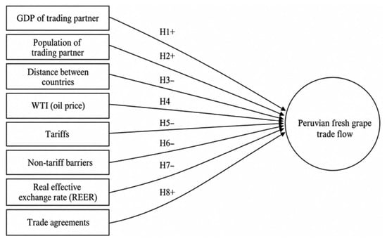
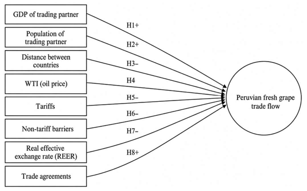
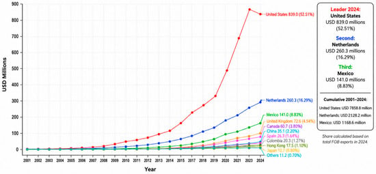
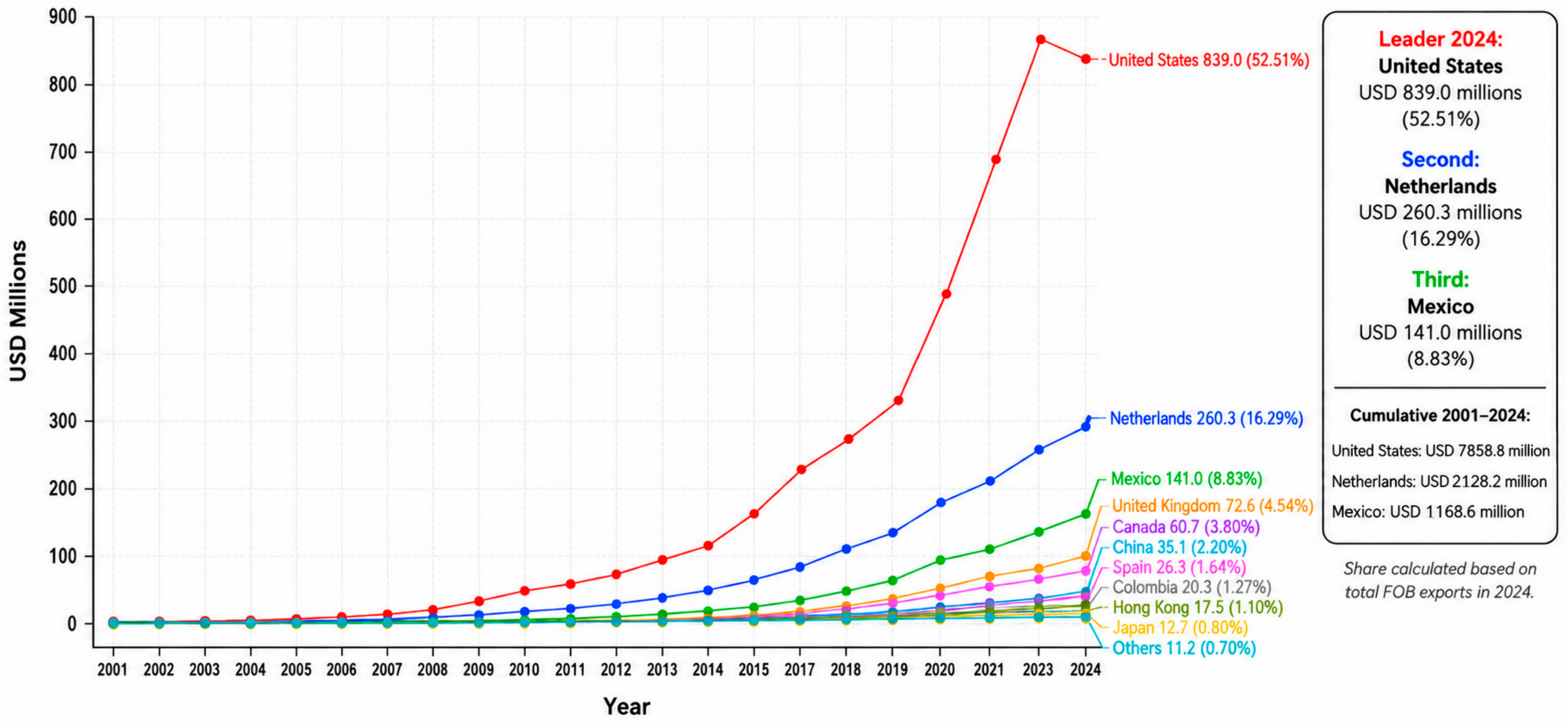
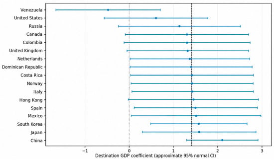
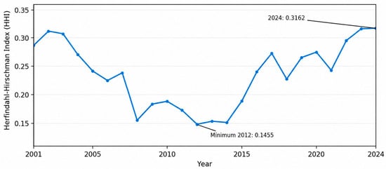

Disclaimer/Publisher’s Note: The statements, opinions and data contained in all publications are solely those of the individual author(s) and contributor(s) and not of MDPI and/or the editor(s). MDPI and/or the editor(s) disclaim responsibility for any injury to people or property resulting from any ideas, methods, instructions or products referred to in the content. |
© 2026 by the authors. Licensee MDPI, Basel, Switzerland. This article is an open access article distributed under the terms and conditions of the Creative Commons Attribution (CC BY) license.