


Abstract
Hard pegs are said to import price stability; floats, to absorb external shocks. Both claims are comparative, yet most evidence comes from single-regime settings. This paper estimates regime differences in inflation transmission on an unbalanced annual panel of commodity-dependent economies, 1990–2024; 71 economies pass the pre-registered audit rule, and 64 contribute the 1722 country-year estimation observations. The frozen design interacts a de facto hard-peg indicator with trading-partner inflation, nominal effective exchange-rate (NEER) growth, and a commodity-orthogonal fiscal-stance measure. Partner inflation is strongly associated with domestic inflation everywhere (coefficient about 0.8), with a difference in the regimes that is not measurable, though this null is imprecisely bounded: imported price pressure is the commodity-exporter norm, not a peg phenomenon. The negative NEER–inflation association is about 0.21 points stronger under hard pegs, or 1.4 additional points of inflation per peg-group standard-deviation NEER move, and the differential survives 39 pre-committed variants. It is identified across economies rather than within them, it is concentrated before 2000, and, as targeted decompositions show, it is carried by the CFA franc zone and largely by the 1994 devaluation; outside that zone the hard-peg differential is small and statistically null, matching the within-switcher estimate. The fiscal-stance and state-dependence interactions are tightly bounded nulls.
Keywords:
hard peg; inflation pass-through; dominant-currency pricing; nominal effective exchange rate; cyclically adjusted fiscal balance; commodity dependence; panel data JEL Classification:
E31; E62; F31; F41; Q02
1. Introduction
Commodity exporters keep returning to the same argument about exchange-rate regimes. A hard peg, one side says, imports the anchor country’s price stability (the classic statement of the evidence is Ghosh et al., 2002); a float, the other side answers, leaves the nominal rate free to absorb external price shocks. Both claims are comparative, in that they are claims about differences between regimes, yet much of the evidence invoked on either side comes from settings with no regime variation at all. Studies of the dollar-pegged Gulf economies, for instance, document strong pass-through of trading-partner inflation to domestic prices, but a single-regime panel cannot say whether that configuration reflects the peg or the region. The raw numbers sharpen the puzzle without settling it: in the panel I assemble below, hard-pegged commodity exporters averaged 3.4 percentage points of inflation over 1990–2024 against 7.1 outside pegs. But the two groups also differ in anchors, income, geography, and history, which is precisely why a level gap identifies nothing by itself. Answering a comparative question requires comparative variation: a panel wide enough to contain hard pegs, intermediate arrangements, and floats, populated by economies exposed to the same class of external price shocks.
This paper builds that panel. The candidate universe is every economy whose UNCTAD-measured commodity-export dependence share averages at least 50 percent over 2021–2023, together with the six Gulf Cooperation Council economies: 115 candidates in all. That cutoff is deliberately more inclusive than the 60 percent threshold UNCTAD itself uses to classify an economy as commodity-dependent (UNCTAD, 2025), and 60 and 70 percent are carried as pre-committed sensitivities. A pre-registered audit rule, fixed before any estimation, admits an economy only if the five core variables are jointly available for at least twenty usable years and its fiscal first stage has at least twenty-five observations; 71 economies survive. Regime classification follows the Ilzetzki–Reinhart–Rogoff de facto codes, which I extend from the IMF’s AREAER for 2020–2024 under documented, source-noted coding rules. One discipline governs everything that follows. The design, comprising the sample rule, variable definitions, baseline specification, inference plan, robustness set, and pre-committed readings of null results, was frozen in writing before the first regression was run on real data.
This paper reaches three findings. First, trading-partner inflation is strongly associated with domestic inflation everywhere: the within-year coefficient is about 0.8 in the interacted model, and the hard-peg interaction is a null. Pass-through of partner prices is the commodity-exporter norm, not a peg phenomenon. Second, the regime-specific result lies in the exchange-rate channel, and it is narrower than a first reading suggests. The association between nominal effective appreciation and inflation is negative everywhere, but it is about 0.21 percentage points stronger per percentage point of appreciation under hard pegs (wild cluster bootstrap p = 0.003), or about 1.4 additional percentage points of inflation per peg-group standard deviation of NEER movement. The differential survives 39 pre-committed robustness variants spanning measurement, specification, sample rules, controls, inference, and regime classification; it is specific to the hardest peg category, concentrated in the pre-2000 decades, and contemporaneous rather than lagged; and under successively broader or announcement-based peg definitions it attenuates and then disappears. Targeted decompositions, reported separately from the pre-committed robustness set, show what that structure means: the differential is carried by the thirteen CFA franc zone economies and, within them, largely by the sixteen CFA country-years of 1994–1995, the years of the January 1994 devaluation. Outside the CFA zone the hard-peg differential is about −0.08 and statistically null, the same magnitude as the within-switcher estimate. What the panel identifies on this channel is a realignment episode inside one hard-peg zone, not a general property of hard pegs. Third, the two channels the theory most expected to differ do not: the peg interaction with commodity-orthogonal fiscal stance and the interaction of partner inflation with the trailing inflation environment are both null under the pre-committed inference protocol. This paper reports these nulls with the same prominence as the positive result, because a channel that does not differ across regimes is itself comparative evidence.
The paper offers three contributions. The first is that it provides, to my knowledge, the first estimates that interact regime status with the partner-price, effective-exchange-rate, and commodity-orthogonal fiscal-stance channels jointly on a broad commodity-exporter panel, with year-fixed effects absorbing common global shocks, an identification structure a single-regime design cannot offer. Regime-conditioned pass-through has been estimated on general cross-country panels, most directly by Ha et al. (2020), and, concurrently with this work, conditioned on the inflation-targeting regime, by Banerjee et al. (2026), but not this channel set, jointly, on this population. Second, it addresses the “peg effect or regional effect” ambiguity left by single-regime studies channel by channel: strong partner-price transmission generalizes across regimes, while the apparent hard-peg amplification of the effective-exchange-rate channel, once decomposed, is a regional and episodic regularity—a result that shows how a binary regime interaction on a broad panel can attribute a single realignment episode to the regime itself. Third, the analysis is conducted under an unusually strict pre-commitment protocol, comprising a frozen design, a pre-registered sample rule, a pre-committed robustness set and null readings, and seeded bootstrap inference, so that the evidential weight of the positive result, and of the nulls, is transparent to the reader.
This study complements Husain (2026), which measures the external-inflation and fiscal-stance channels within the six dollar-pegged GCC economies. Two construction methods are adopted from that work, with citation: the trade-weighted partner-inflation measure (there applied to GCC importers) and the commodity-orthogonal cyclically adjusted fiscal residual (there estimated against the Brent price, here generalized to country-specific commodity export-price indices). Everything else is new—the sample (71 economies rather than six), the question (regime conditioning rather than within-regime measurement), the identification structure (a wide cross-section that admits year-fixed effects and regime interactions), and every estimate, table, and figure. The GCC point estimates from that paper appear below only as cited benchmarks in the Discussion; I never re-derive them from the present panel.
The paper proceeds as follows. Section 2 situates the question in four sections of the literature and states the hypotheses; Section 3 describes the sample rule, variable construction, and estimation sample; Section 4 sets out the specification, the inference plan, and the identification limits; Section 5 presents the results and the robustness set; Section 6 reports heterogeneity and state dependence; Section 7 discusses interpretation, the GCC benchmark, policy, and limitations; and Section 8 presents conclusions.
2. Literature and Hypotheses
2.1. Regime Classification and Macroeconomic Outcomes
The measurement apparatus comes first. Reinhart and Rogoff (2004) reconstruct the modern history of de facto exchange-rate arrangements and show that announced and actual regimes routinely diverge; Ilzetzki et al. (2019, 2022) carry the classification into the recent period, document the dollar’s enduring dominance as an anchor, and provide the fine and coarse codes I use here. Shambaugh (2004) shows that pegs measurably surrender monetary autonomy, with local interest rates tracking the base country, which is the mechanism behind the imported-monetary-stance logic I invoke below; and Levy-Yeyati and Sturzenegger (2005) demonstrate that deeds-based classification changes inference relative to words-based classification. Klein and Shambaugh (2010) synthesize the accumulated evidence, finding that pegs buy modest inflation benefits at a measurable cost in monetary autonomy, and their emphasis on long, stable spells motivates the spell-length sensitivity I incorporate below. What this literature largely does not do is interact regime status with imported-price and fiscal channels on a commodity-exporter panel. Regimes appear as outcomes, or as conditioning variables for growth and volatility; on commodity-exporter panels they are rarely treated as moderators of inflation transmission. That is the gap this research occupies.
2.2. Pass-Through and Dominant-Currency Pricing
How external prices reach domestic inflation is the second area of the literature. Taylor (2000) argues that pass-through is an equilibrium object that weakens in low-inflation environments, and Choudhri and Hakura (2006) confirm the inflation-environment regularity across countries. The dominant-currency paradigm of Gopinath et al. (2020) sharpens the regime implication: when trade is invoiced in dollars, the bilateral dollar rate governs border prices, so pegging to the dollar stabilizes import prices in local currency and shifts the operative external channel from the own exchange rate toward partner prices and dollar-denominated costs. Forbes et al. (2018; cross-country in 2020) add a caution I will need: measured pass-through depends on which shock moves the exchange rate, and the composition of shocks behind effective-rate movements differs mechanically between peggers—whose multilateral rate is inherited from the anchor’s cross-rates—and floaters, whose rate also responds to domestic conditions and policy. Closest to this paper’s design, Ha et al. (2020) estimate pass-through for 47 countries and show that it moves with the shock behind the currency change and with country characteristics, the policy framework included; regime there moderates the exchange-rate channel on a general panel. These predictions are comparative across regimes. They are rarely tested jointly, channel by channel, on the economies for which the peg debate is most alive: commodity exporters.
2.3. Fiscal Policy and Inflation in Commodity Exporters
The third section of the literature concerns the fiscal–macro nexus of commodity exporters. Barnett and Ossowski (2002) set out the operational problem: revenue is volatile, cyclical, and largely outside the government’s control. Céspedes and Velasco (2014) document procyclical fiscal responses to commodity booms and their macroeconomic costs; Erbil (2011) finds the procyclicality concentrated in developing oil producers; and Gruss and Kebhaj (2019) provide the country-specific commodity terms-of-trade indices I use to price each economy’s export basket. The persistent measurement difficulty in this literature is discretionary stance, because headline balances inherit the commodity cycle. The commodity-orthogonal residual I use below—the component of the fiscal balance orthogonal to current and lagged export prices—addresses the difficulty with minimal data requirements, and the trilemma logic of Section 2.1 supplies the comparative hypothesis: under a peg, with monetary policy imported, fiscal stance is the domestic stabilization margin, so its association with inflation could plausibly be stronger.
2.4. The Single-Regime Benchmark
Finally, Husain (2026) quantifies the external-inflation and fiscal-stance channels within the six dollar-pegged GCC economies and documents a structural weakening of the external association after the 2014 oil price collapse. That design measures the configuration inside one regime. By its construction, it cannot say whether the configuration is regime-specific—and embedding the question in a wide cross-regime panel, as I do here, is precisely what turns the within-regime measurement into a comparative test.
2.5. Hypotheses
The literature above yields four comparative hypotheses, fixed in the frozen design before estimation and derived from theory rather than from anticipated estimates.
H1 (dominant-currency pricing).
The association between trading-partner inflation and domestic inflation is larger under hard pegs to the dominant invoicing anchor than under floats, conditional on controls.
H2 (trilemma float logic).
The exchange-rate (NEER) channel is correspondingly larger under floats, whose nominal rates are free to move and absorb shocks.
H3 (imported monetary stance).
The negative association between commodity-orthogonal fiscal stance and inflation is stronger under pegs, where no independent monetary reaction offsets fiscal impulses.
H4 (Taylor-type state dependence, secondary).
External-price transmission strengthens in high-inflation environments, measured by the trailing three-year own-inflation mean.
Each hypothesis is comparative, and each is evaluated under the pre-committed inference protocol of Section 4, with null readings specified in advance. Section 5 evaluates H1–H3, Section 6.2 evaluates H4, and Section 7 returns to each.
3. Data and Sample
3.1. Candidate Universe and Pre-Registered Sample Rule
The candidate universe is the union of economies with an UNCTAD-measured commodity-export dependence share of at least 50 percent (averaged 2021–2023, from the frozen 2025 extract; Section 1 notes the relation to UNCTAD’s own 60 percent classification threshold) and the six GCC economies: 115 candidate reporters. Admission is governed by an audit rule fixed in the frozen design before any regression was run. An economy enters if and only if (i) the five core variables—CPI inflation, partner inflation, commodity export-price growth, regime classification, and the WEO fiscal balance—are jointly non-missing in at least 20 usable years, where a usable year requires a de facto regime in the four ordinary coarse categories (excluding freely-falling and dual-market years) and absolute inflation of at most 50 percentage points; and (ii) the country’s fiscal first stage (Section 3.2) has at least 25 observations. I emphasize that the rule, not the resulting list, is the frozen object.
Seventy-one economies survive. The attrition ledger is mechanical: 115 candidates; 111 with regime coverage; 73 with at least 20 usable years; and 71 after the first-stage rule. All six GCC economies are among the survivors. Near-misses with 15–19 usable years are listed in the audit log; the rule was never relaxed to admit a country. Because a country can sit on both sides of the peg indicator over 35 years, side counts use both-sides counting with a five-usable-year floor: 45 economies contribute hard-peg years and 47 contribute non-peg years within the panel frame, and eleven economies switch hard-peg status at least once during the sample (twelve within the Section 3.3 estimation sample). Table 1 reports the sample construction and regime composition; Figure 1 maps hard-peg status by country and year, including the Author-coded 2020–2024 extension.
Table 1.
Sample construction and regime composition.
Figure 1.
Hard-peg status of the survivor panel by country-year, 1990–2024. Each row is one of the 71 survivor economies, ordered by hard-peg share; dark cells are hard-peg years (IRR coarse category 1, PEG1 = 1), light cells are other usable regime years (coarse categories 2–4), and blank cells lie outside the usable sample. Classifications for 2020–2024 are the Author-coded AREAER extension described in Section 3.2. Source: Author’s calculations.
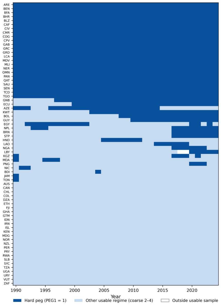
Table 2.
Descriptive statistics, estimation sample.
3.2. Variable Construction
Dependent variable. I take CPI inflation in percentage points from the World Development Indicators. Country-years with absolute inflation above 50 percentage points are excluded from the baseline, a Cagan-style screen (Cagan, 1956) that removes hyperinflationary observations whose dynamics are not the object of this paper, with a pre-committed no-cut sensitivity. For two GCC members whose WDI series begin after 1990 (the United Arab Emirates before 2008 and Oman before 2001), I splice the pre-WDI years from WEO period-average CPI actuals; the overlap correlation between the two sources is 0.905 for the UAE (mean absolute deviation 0.416 pp) and 0.999 for Oman (0.084 pp); the spliced observations are flagged in the panel, and a no-splice sensitivity is pre-committed.
Regime classification. De facto regimes are the Ilzetzki–Reinhart–Rogoff fine codes, collapsed to the standard six coarse categories with the published fine-to-coarse mapping and validated cell-by-cell against the published coarse sheet. I use published annual codes through 2016; for 2017–2019 I collapse the monthly classification by modal category with a December tiebreak, a convention that agrees with the published annual codes in 89.7 percent of 5214 overlapping country-years (against 87.4 percent for December-only). For 2020–2024 I extended the classification from the IMF’s Annual Report on Exchange Arrangements and Exchange Restrictions under fixed rules: the AREAER edition of year Y + 1 codes year Y, a majority-of-year rule governs within-year changes, and a freely-falling screen at 40 percent annual CPI is applied from the frozen WDI series. Each of the 355 extension country-years carries a source note, and the underlying AREAER chapter documents and the full revision history of the classification are retained. The baseline peg indicator PEG1 equals one for coarse category 1 (hard pegs); a broader PEG12 indicator (coarse ≤ 2) is a pre-committed sensitivity. Anchor-currency identity (USD versus other) follows the same source, and an inflation-targeting dummy is constructed from an Author-compiled chronology of formal IT adoption among the survivors (15 adopters; 341 IT country-years), each adoption year backed by a filed central-bank or IMF source.
Partner inflation. For every candidate reporter, I compute partner inflation as the trade-weighted average of partners’ WDI CPI inflation, with weights equal to the reporter’s bilateral import shares from IMF trade statistics over a strictly backward-looking trailing five-year window (t − 5 to t − 1), using positive import flows only. Aggregate counterparts are removed by IMF partner code. Partner-years with CPI inflation above 50 percentage points are excluded with weight renormalization, mirroring the dependent-variable screen. The baseline uses all-partner rolling weights; ex-GCC, fixed-weight (2010–2019 average shares), and no-hyperinflation-cut variants are carried as pre-committed sensitivities.
Commodity export prices. Country-specific commodity export-price growth comes from the IMF’s commodity terms-of-trade database (Gruss & Kebhaj, 2019). The rolling-weight export index is the baseline, with fixed-weight and export-plus-import variants carried; growth rates are year-over-year in percentage points. The point of the country-specific index is simple: it replaces any single global price with each economy’s own export basket.
Effective exchange rate. I compute nominal effective exchange-rate growth from the Bruegel database (Darvas, 2012; 16 July 2026 update), using the 170-partner basket where consecutive years exist and the 65-partner basket otherwise (binding in 1990–1992 and for late starters; 507 filled country-years, flagged). Positive values denote appreciation.
Fiscal balance and commodity-orthogonal stance. The fiscal balance is the WEO general-government net lending/borrowing ratio to GDP, actual observations only (as delimited by each vintage’s last-actual marker), with fiscal-year labels mapped by leading calendar year. I measure discretionary stance by a commodity-orthogonal residual estimated country by country: the balance is regressed on a constant and the current and lagged commodity export-price index, in levels, and the residual, denoted CAF (the commodity-orthogonal cyclically adjusted fiscal residual; not the ISO code of the Central African Republic used in Table A1), serves as the stance measure, with Newey–West (three-lag) first-stage covariances stored for the bootstrap of Section 4.2. First stages are estimated for every economy with sufficient data, and a country’s CAF is used only where the first stage has at least 25 observations. The construction generalizes that of Husain (2026) from a single global oil price to country-specific export baskets; the survivor first stages are reported in Appendix B. Fit varies widely: seventeen of the 71 survivor R2 values fall below 0.05 (median 0.124). For those economies CAF is close to the demeaned balance itself, and the fiscal-stance nulls below are read with that in mind.
Controls and drivers. Baseline controls are government consumption over GDP, broad money growth, real GDP growth, the Chinn–Ito capital-account openness index (Chinn & Ito, 2006), and the inflation-targeting dummy. The 2024 value of the Chinn–Ito index, unreleased at freeze time, is carried forward from 2023 per country under a flagged release-lag convention, with a pre-committed no-carry sensitivity. Year-fixed effects absorb common global conditions in the baseline; a pre-committed no-year-fixed-effects variant replaces them with observable global drivers—the federal funds rate, a high-frequency monetary-surprise measure (Bauer & Swanson, 2023), a global real-activity index, equity volatility, and Brent growth—each rebuilt from frozen sources before that variant was estimated.
3.3. Estimation Sample and Descriptive Statistics
Applying the baseline regressor set as a complete-case rule to the 71 survivors on the 1990–2024 frame yields 2485 survivor country-years, of which 2206 are usable under the regime and inflation screens. Requiring the three controls with imperfect coverage, namely government consumption, broad money, and the capital-account index, leaves an estimation sample of 1722 country-years across 64 economies, the cluster count for inference. Seven survivors contribute no baseline rows, solely because of control gaps. Two pre-committed sensitivities restore them: a parsimonious-control variant (dropping government consumption and broad money; 2153 rows, 70 clusters) and a gated splice of the government-consumption series from the UN Main Aggregates Database (Section 5.5). No conclusion, therefore, rests on their exclusion. Within the estimation sample, 697 country-years are hard-peg and 1025 are not. Table 2 reports descriptive statistics, and two contrasts stand out. Mean inflation is 3.4 percentage points under hard pegs against 7.1 outside them. Mean NEER growth is mildly positive under pegs (+1.1 percent) against mildly negative outside (−1.5 percent), with a visibly smaller NEER standard deviation under pegs (6.8 against 9.8). This is compressed, but far from degenerate, multilateral variation, and it is this variation that identification of the exchange-rate interaction relies on.
4. Empirical Strategy
4.1. Specification
The baseline is a two-way fixed-effects regression with regime interactions:
where π is CPI inflation, PARTNERπ is partner inflation, ΔNEER is nominal effective appreciation, ΔPX is commodity export-price growth, CAF is the commodity-orthogonal fiscal residual, M collects the remaining controls, αi and λt are country and year effects, and Z ranges over {PARTNERπ, ΔNEER, CAF}. The three interaction coefficients θj are the parameters of interest: they measure regime differences in conditional transmission associations. I estimate progressively, with Model 1 omitting the interactions and Model 2 adding them, and pre-committed alternatives replace the binary peg with fine and coarse regime categories, add anchor-specific interactions, drop year effects in favor of observed global drivers, add lagged inflation, difference the specification, and lag the external drivers as a timing check. I conducted no specification search of any kind; every reported variant was fixed in the frozen design or by dated pre-estimation amendment, including the decompositions of Section 5.6 (frozen-design document and amendment log in the Supplementary Materials, File S1).
πit = αi + λt + β1 PARTNERπit + β2 ΔNEERit + β3 ΔPXit + γ1 CAFit + γ2 GOVCONSit + δ′Mit + Σj θj (PEGit × Zit,j) + εit
4.2. Inference
This paper clusters the tabulated primary standard errors by entity (CR1) over the 64 sample economies, and I report the Driscoll and Kraay (1998) covariance as co-primary, since it is robust to both cross-sectional and serial dependence. For the three headline interaction terms, I compute a restricted (null-imposed) wild cluster bootstrap with Webb six-point weights (Cameron et al., 2008; Webb, 2023; Roodman et al., 2019), with B = 9999 replications and a fixed seed, and I treat it as the most reliable guide where methods disagree. Throughout, CR1 denotes the entity-clustered covariance computed without the G/(G − 1) small-sample factor, with t-statistics referred to the standard normal; Section 5.2 reports how the headline p-value moves under the conventional factor and a t(G − 1) reference. Because CAF is a generated regressor, its own coefficient γ1 is additionally assessed with a two-stage bootstrap that re-estimates the first stages inside each replication—under both a parametric-joint and a block-wild-joint design; the two-stage designs are not extended to the PEG1 × CAF interaction (Section 7.4, fourth limitation).
4.3. Identification and Its Limits
The regime contrasts in this paper are associations, not causal effects, and I frame them as such throughout. Regime choice is not random: economies choose anchors in light of their inflation histories, institutions, and trade structures, and twelve estimation-sample economies switch hard-peg status within the window—enough to attempt the within-switcher estimator of Section 5.3, not enough for within-country identification of the contrast to carry the paper. The headline θj are therefore identified primarily from cross-sectional differences in slopes among economies observed under different regimes, conditional on country and year effects and the control set. What the design does deliver is discipline on the alternative explanations. Year effects absorb common global shocks that could otherwise masquerade as regime differences; commodity export prices and partner inflation are externally priced for small exporters, with a price-taker subsample excluding the five largest exporters as a check; controls hold inflation-targeting adoption and capital-account openness fixed; a long-spell subsample restricts to regimes in place at least ten years, reducing switch-related contamination; and within-spell estimates re-express the contrast using only variation inside continuous regime episodes. What the design cannot do is rule out that unobserved, slope-relevant country characteristics correlate with regime choice. Section 7 returns to this squarely.
5. Results
5.1. Baseline Associations
Table 3 reports the progressive build. I take Model 2, with the interactions, as the reference specification for interpretation; Model 1 shows the external channels before the interactions enter, and it behaves exactly as the single-regime literature leads one to expect on a commodity-exporter panel. Partner inflation carries a coefficient of 0.661 (CR1 p < 0.001; Driscoll–Kraay p < 0.001): roughly two-thirds of partner price growth is matched in domestic inflation within the year, conditional on country and year effects. Nominal effective appreciation is negatively associated with inflation (−0.170, CR1 p < 0.001). Commodity export-price growth is a null once partner inflation and year effects are present, and the commodity-orthogonal fiscal residual is likewise null in this panel (−0.016, CR1 p = 0.598)—a first indication that the fiscal-stance channel documented within single-regime settings does not generalize unconditionally. Broad money growth enters positively, and the hard-peg level term is −1.938 (CR1 p = 0.027): conditioning roughly halves the unconditional 3.7-point gap of Table 2.
Table 3.
Baseline and headline interaction estimates.
5.2. The Headline Interactions
Model 2 adds the three regime interactions, and two of the three are null. The partner-inflation interaction θ1 is −0.194 with a CR1 p-value of 0.196 and a restricted wild-bootstrap p-value of 0.238: the point estimate is, if anything, mildly negative, the opposite of H1’s prediction, and the confidence set contains zero, though it is wide (Section 5.7). The fiscal interaction θ3 is 0.020 (bootstrap p = 0.797); H3 finds no support, and γ1 itself remains null under both two-stage bootstrap designs. Partner inflation’s level coefficient rises to 0.803. Strong pass-through of partner prices, in short, is the cross-regime norm.
The exchange-rate interaction is where the regimes differ in the full panel. The estimate is θ2 = −0.212 (CR1 p = 0.001; Driscoll–Kraay p = 0.045; restricted Webb wild-bootstrap p = 0.003): the negative association between effective appreciation and inflation is about 0.21 percentage points stronger, per percentage point of appreciation, under hard pegs than outside them—on top of a non-peg slope of −0.118. Under the CR1 convention of Section 4.2 the p-value is 0.0006; applying the conventional G/(G − 1) factor with a t(63) reference gives 0.001, and no headline term changes significance category under that convention. This is the reverse of H2, which expected that the exchange-rate channel would belong to the floaters. The magnitudes are worth stating in standard-deviation units. Evaluated at each group’s own dispersion, one standard deviation of NEER growth is associated with 1.16 percentage points of inflation in the non-peg group (SD 9.8) and, under hard pegs (SD 6.8), with an additional 1.45, for a total of 2.25 percentage points, β2 + θ2 = −0.330; at the pooled dispersion of 8.8 points the non-peg association is 1.04 and the additional hard-peg association 1.87 (standardized β = −0.295), and the own-group figures are the ones used elsewhere in the paper. By comparison, one standard deviation of partner inflation (2.1 pp) is associated with 1.65 points, with a regime differential of −0.40 that is statistically null. Figure 2 previews the stability of this contrast across the pre-committed robustness set developed in Section 5.5; Section 5.6 reports the targeted decompositions that locate the differential in the CFA franc zone.
5.3. Estimates by Regime Status, and Within Switchers
Table 4 splits the headline equation by regime status. This is a descriptive decomposition, not a within-episode estimator: 52 of the 64 sample economies appear on one side of the split only, so the contrast between columns is still carried mainly by cross-country variation. Within hard-peg rows (697 country-years, 34 clusters) the NEER–inflation association is −0.362 (CR1 p < 0.001); within float and intermediate rows (1025 country-years, 42 clusters) it is −0.110 (p = 0.020). The split-sample slopes and the pooled interaction model reconcile as follows: the peg-side slope of −0.362 corresponds to β2 + θ2 = −0.330 in Table 3, and the implied split differential of −0.252 to θ2 = −0.212, the gaps arising because the split lets every control slope and both sets of fixed effects differ by regime, whereas the pooled model lets only the three interacted slopes do so; the coarse-1 row of Table 5 (−0.204) is a differential of the second kind. The partner-price channel is strong on both sides (0.514 and 0.740), with no sign of peg amplification, and the fiscal residual is null in both columns; the inflation-targeting control drops mechanically on the peg side, where it has no within variation. The within-country version of the contrast is estimated separately, on the twelve economies observed on both sides of PEG1 inside the estimation sample: the differential there is −0.076 (CR1 SE 0.070, p = 0.282; restricted Webb wild-bootstrap p = 0.325; N = 321, 12 clusters), and restricting further to rows inside regime spells of at least five years gives 0.006 (p = 0.954). The switcher estimate carries the same sign as the headline but little of its strength, and with twelve clusters it is imprecise by construction. I therefore state the identification plainly: the headline differential is a cross-sectional regularity among economies observed under different regimes; the within-switcher evidence is directionally consistent and statistically limited; and Section 5.6 shows that the cross-sectional regularity is itself concentrated in one group of economies.
Figure 2.
The headline contrast across the pre-committed robustness set. Point estimates of θ2 (PEG1 × ΔNEER) with 95% CR1 confidence intervals for the baseline (diamond) and each pre-committed variant of Table 5 (circles); the vertical line marks zero. The Driscoll–Kraay and two-way-cluster rows of Table 5 are omitted because they repeat the baseline point estimate under alternative inference. Source: Author’s calculations.
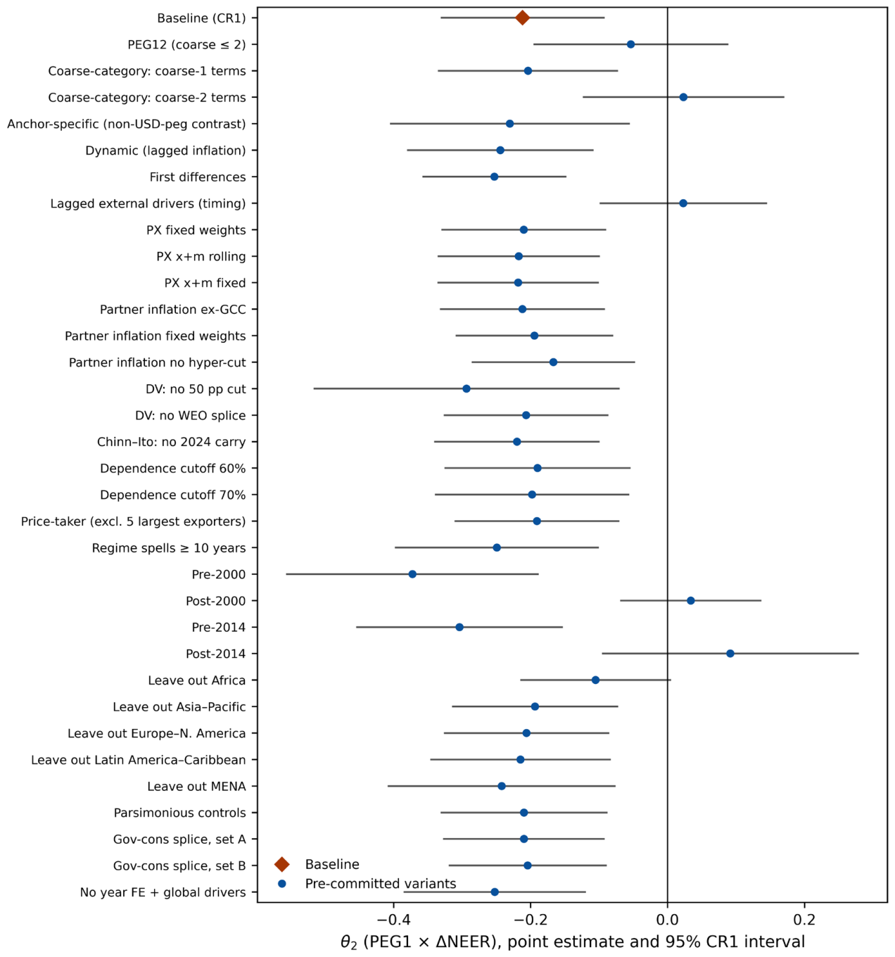
Table 4.
Estimates by regime status.
Table 5.
Pre-committed robustness set: the three regime interactions across 39 variants (panel a), and the classification ordering on common samples (panel b).
5.4. Diagnostics
The pre-committed diagnostics support the specification. Residual cross-sectional dependence is absent once year effects are in place: the Pesaran CD statistic is −1.46 (p = 0.146) for Model 1 and −1.46 (p = 0.145) for Model 2 (Pesaran, 2021). Panel unit roots are rejected at p < 0.001 for all four core series by Maddala–Wu and Choi combination tests (Maddala & Wu, 1999; Choi, 2001; Im et al., 2003 for the framework), computed over the 60 economies with sufficient span. A Wooldridge-type test (Wooldridge, 2010; Drukker, 2003) documents positive serial correlation in the idiosyncratic errors, as expected in annual inflation data; the CR1 and Driscoll–Kraay covariances accommodate it, and the pre-committed dynamic variant addresses it directly (Section 5.5), the usual Nickell (1981) caveat being the reason the dynamic form is a robustness line rather than the baseline. Variance inflation is modest (maximum VIF 2.90, on the partner-inflation interaction). A leave-one-country-out sweep moves θ2 only within [−0.237, −0.182] with no sign flips on θ1 or θ2, and at the observation level no single country-year moves θ2 outside [−0.262, −0.186] (the extreme is Libya 2021); θ3 crosses zero under some drops, exactly as a null should.
5.5. Robustness
Table 5 reports the full pre-committed robustness set, specifically, the baseline and 39 pre-committed variants spanning inference, classification, dynamics, measurement, sample rules, and controls, every row fixed before estimation (the decompositions of Section 5.6 are reported separately). Three regularities organize the table. The first is stability across the measurement, specification, sample-rule, control, and inference rows: there, θ2 lies between −0.17 and −0.29; it is significant at the 1 percent level under CR1 and the restricted wild bootstrap, at 5 percent under Driscoll–Kraay, and at 10 percent under two-way clustering (p = 0.056), and it retains CR1 significance across alternative commodity-price measures (fixed weights; export-plus-import baskets), alternative partner-inflation constructions (ex-GCC; fixed weights; and no hyperinflation cut), the no-50-point inflation cut, the no-splice dependent variable, the no-carry capital-account rule, tighter dependence cutoffs (60 and 70 percent), the price-taker subsample excluding the five largest exporters, long regime spells, the dynamic and first-difference specifications, the parsimonious-control sample (70 clusters), both government-consumption splice sets, the anchor-currency-by-year-fixed-effects variant (−0.230, CR1 p = 0.013), and the no-year-fixed-effects variant with observed global drivers; a country jackknife gives t = −3.11.
The second regularity is informative structure, which I report rather than suppress. The contrast is specific to the hardest pegs: the coarse-category specification reproduces it for coarse-1 (−0.204, p = 0.002) while the coarse-2 interaction is zero, and diluting the peg group with coarse-2 economies (PEG12) eliminates it (−0.054, p = 0.461). Panel (b) of Table 5 sets out the classification ordering on common samples. Replacing PEG1 with the Shambaugh strict peg on the 1990–2018 overlap attenuates the differential to −0.111 (p = 0.205), against −0.284 (p < 0.001) for the frozen classification on identical rows, a plain non-confirmation under that coding; on the same 1418 rows the PEG12 dilution gives −0.071 (p = 0.373), so the common-sample ordering is −0.284 → −0.111 → −0.071. The attenuation is definitional widening of the peg group rather than contested observations: the two codings agree on 89.8 percent of the 1418 estimation rows, with disagreement running 119-to-25 toward additional Shambaugh peg calls, and on the agreement-only rows the frozen-classification differential is −0.283 (p < 0.001). Replacing PEG1 with the announced (de jure) AREAER peg on the 2000–2022 overlap yields +0.230 (p < 0.001), with the frozen-classification companion on identical rows at +0.091 (p = 0.055): in the post-2000 window announced status carries, if anything, the opposite-signed association. The differential is concentrated in the earlier decades, −0.373 (p < 0.001) before 2000 and −0.304 before 2014 against nulls after 2000 and after 2014, and the pre-committed formal contrast confirms the split: adding POST-2001 interactions to the headline equation, the PEG1 × ΔNEER × POST coefficient is +0.387 (CR1 p < 0.001; Driscoll–Kraay p < 0.001; restricted Webb wild-bootstrap p = 0.005), with a pre-2001 differential of −0.385 and an implied post-2001 differential of essentially zero. Read jointly: the differential lives in the pre-2000 decades, where the announced-regime coding is unavailable and the one alternative behavioral coding attenuates it; in the post-2000 window, where both codings exist, neither shows a negative differential. It is attenuated most by removing Africa (−0.105, p = 0.062) in the leave-one-region-out sweep, and in the anchor-specific specification the non-USD-peg contrast carries the effect (−0.230, p = 0.010). And it is contemporaneous: lagging the external drivers by one year eliminates it (0.023, p = 0.712). Taken one at a time, each of these facts admits several readings; Section 5.6 shows that they share one. The third regularity is that the nulls are stable too. The θ1 and θ3 remain null in essentially every row, with isolated cells reaching p < 0.05 across the 40 rows of Table 5: the lagged-driver θ1, the no-year-fixed-effects θ1, and one leave-one-region θ3. The first two share a feature worth naming rather than suppressing: both alter the treatment of common global shocks. Under the multiplicity discipline none of the three is treated as a finding, but the recurrence marks the partner-price interaction as the cell to watch in designs that model, rather than absorb, the global cycle.
5.6. Decomposing the Differential
Three targeted checks that the frozen design did not anticipate are reported here, in Table 6 and Figure 3, separately from the pre-committed robustness set; each was fixed before it was estimated, and none alters a row of Table 5. All use the baseline specification, control set, fixed effects, and inference conventions.
Table 6.
Decomposing the hard-peg NEER differential: targeted checks.
Figure 3.
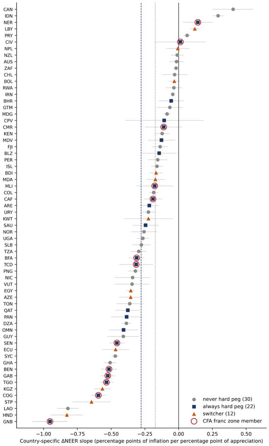
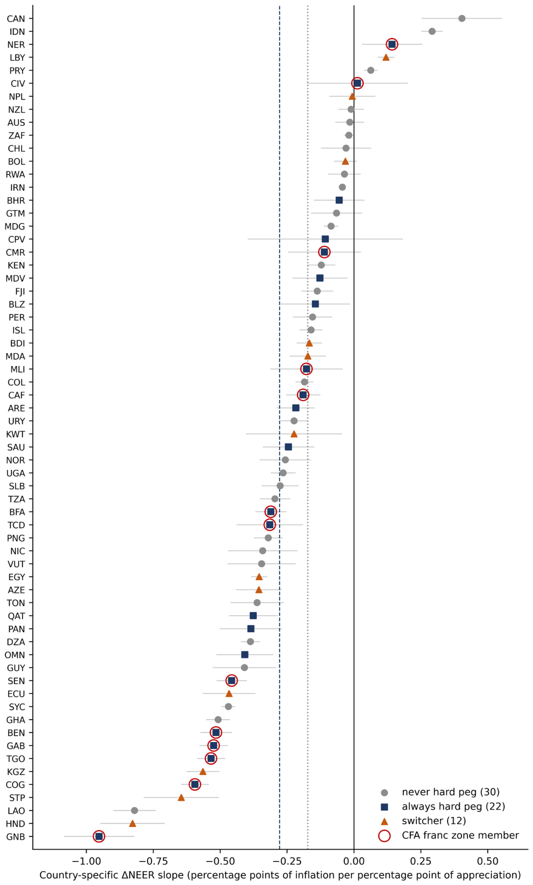
Country-specific ΔNEER slopes from the headline equation. One slope on nominal effective exchange-rate growth (ΔNEER) per economy (64 economies) replaces the level and hard-peg interaction terms of the headline equation, with all other regressors and both sets of fixed effects retained; economies (ISO-3 codes) are ordered by slope. Markers: squares = always-hard-peg (22), circles = never-hard-peg (30), triangles = hard-peg switcher (12); red rings mark the thirteen CFA franc zone members. Horizontal bars are 95% entity-clustered (CR1) intervals and are descriptive only, each slope being identified within a single cluster. The solid vertical line marks zero; the dashed line marks the median slope of the always-hard-peg economies (−0.278) and the dotted line the median of the never-hard-peg economies (−0.173). Source: Author’s calculations.
The first check concerns the CFA franc zone. Thirteen survivor economies are members, and in the estimation sample every one of their 366 country-years is a hard-peg year, so they supply 366 of the 697 hard-peg rows (53 percent) and 86 of the 150 hard-peg rows before 2000. For these economies, the effective rate is the CFA franc’s cross-rate, and the January 1994 devaluation produced, inside the pre-2000 window, declines in the effective rate of 39 to 47 percent, alongside inflation of about 25 to 42 percentage points in the seven members whose 1994 observations enter the sample—a cluster of simultaneous observations that the one-at-a-time influence sweep of Section 5.4 cannot detect. Excluding the thirteen economies, θ2 falls to −0.074 (CR1 p = 0.225; restricted Webb wild-bootstrap p = 0.269; N = 1356, 51 clusters); excluding only the sixteen CFA country-years of 1994–1995 gives −0.099 (p = 0.157; bootstrap p = 0.194); excluding 1994–1995 for all economies gives −0.098 (p = 0.141; bootstrap p = 0.170). Because every CFA row is a hard-peg row, a CFA × ΔNEER term added to the headline equation partitions θ2 exactly: the non-CFA hard-peg differential is −0.077 (p = 0.207; bootstrap p = 0.245) and the CFA increment −0.260 (p = 0.004; bootstrap p = 0.029), for a CFA hard-peg differential of −0.337. In the pre-2000 cell without the CFA economies, the differential is +0.040 (p = 0.807; bootstrap p = 0.605; N = 335, 46 clusters). The full-panel differential is, in short, a CFA-zone regularity, and largely a 1994 regularity; outside the zone the hard-peg differential is about −0.08, statistically null, and of the same magnitude as the within-switcher estimate of Section 5.3.
The second check concerns measurement in the early sample. Eighty-four estimation rows, all before 2000 and 26 of them hard-peg years, carry the 65-partner backfilled effective rate. Removing them, the pre-2000 differential is −0.422 (p < 0.001; bootstrap p = 0.001; N = 337); estimating the pre-2000 cell on the 65-partner series throughout gives −0.323 (p = 0.002; bootstrap p = 0.011); and removing the backfilled rows from the full sample gives −0.227 (p < 0.001; bootstrap p = 0.002). The backfill does not carry the result.
The third check concerns timing and the shape of the cross-country distribution. A distributed-lag version of the headline equation, with ΔNEER and partner inflation at t, t − 1, and t − 2, each interacted with PEG1 (N = 1668), shows that, outside hard pegs, the exchange-rate association builds over a year (−0.07 at t; −0.17 at t − 1, p < 0.001; zero at t − 2; cumulative −0.24), whereas the hard-peg differential is contemporaneous (−0.28 at t; −0.01 and −0.08 at the two lags; cumulative three-year differential −0.37, bootstrap p = 0.003), and that partner-inflation transmission is contemporaneous for everyone. Re-estimated without the CFA economies, the peg differential is −0.08 at t and −0.22 cumulatively (bootstrap p = 0.110); the immediacy is the 1994 realignment. Finally, replacing the binary interaction with one ΔNEER slope per economy (Figure 3) shows a continuum rather than two points. The 22 always-peg economies have a mean slope of −0.30 against −0.19 for the 30 never-peg economies (mean-group difference −0.11, p = 0.093); without the CFA members the peg mean is −0.23 and the difference −0.04 (p = 0.485). Six CFA members sit in the negative tail of the distribution; the other seven are spread across its middle.
The fiscal channel was re-examined in the same way; the estimates appear in Table 6 and are discussed in Section 7.2. Restricting the sample to economies whose fiscal first stage has an R2 of at least 0.05 or 0.10 leaves θ3 null (+0.076, p = 0.124; +0.100, p = 0.081), and replacing CAF with the WEO headline balance leaves both the level and the interaction null (−0.021 and +0.024; p = 0.631 and 0.651), with θ2 unchanged.
5.7. Reading the Hypotheses
Where does this leave the hypotheses? Under the pre-committed protocol, H1 is not supported, and the null is imprecise: the 95 percent CR1 interval for θ1 is [−0.49, +0.11] (minimum detectable effect 0.42 against a level coefficient of 0.80), so regime differences of substantive size are not ruled out in either direction. H2 is not supported: in the full panel the exchange-rate differential is opposite in sign to the prediction, and the decompositions of Section 5.6 locate that differential in the CFA franc zone; outside it, the channel does not differ measurably by regime. H3 is not supported, and this null is tight: θ3’s interval is [−0.10, +0.14] (minimum detectable effect 0.17), as is the H4 interaction of Section 6.2. This paper specified these readings in advance for the null and mixed cases, and I state them plainly here, because a transmission configuration that is not regime-specific on a given channel is itself evidence against comparative dominant-currency and trilemma priors, evidence to be reported rather than repackaged.
6. Heterogeneity and State Dependence
6.1. Moderation of the Headline Contrast
Does the hard-peg NEER differential vary across types of economies? This paper fixed four moderators in advance—World Bank income group (frozen single vintage, collapsed to high/upper-middle versus low/lower-middle), fuel versus non-fuel export dependence (UNCTAD strict-maximum product-group rule), commodity-dependence terciles (within-survivor terciles of the frozen dependence measure), and anchor currency (USD versus non-USD)—and two devices keep the analysis honest. Descriptive subsample re-estimations of the headline equation are reported per cell, under the pre-committed discipline that a coefficient significant in one cell and not another is not evidence of a difference; and the sole formal test per moderator is a triple interaction PEG1 × ΔNEER × G on the full sample, the four tests declared as a single family with Romano–Wolf stepdown p-values from a common-draw wild cluster bootstrap (Romano & Wolf, 2005; Clarke et al., 2020).
Table 7 reports both layers. In the cells, θ2 is negative in all nine subgroups, covering high- and low-income economies, fuel and non-fuel exporters, every dependence tercile, and USD and non-USD anchors; small-cell wild-bootstrap checks are applied where cluster counts fall below thirty. Two isolated cells, the USD-anchor θ1 and the middle-tercile θ3, reach p < 0.05, and are read under the same discipline. In the formal family, all four triple interactions are null: unadjusted bootstrap p-values range from 0.396 to 0.975, and every Romano–Wolf p-value is at least 0.89. I read the two layers together with the decompositions of Section 5.6. The four moderators were fixed before estimation, and none of them isolates the CFA franc zone: its thirteen members enter both income cells, both export types, and all three dependence terciles, so the cells provide no evidence that the differential is carried by income level, export type, or dependence intensity as such. The anchor moderator is different in kind. Every CFA country-year carries a French franc or euro anchor, and the 366 CFA rows make up more than half of the 652-row non-USD-anchor cell, which is why that cell (−0.302, CR1 p = 0.008) is the strongest: the descriptive anchor pattern is the CFA pattern seen from another side, not evidence about the dollar cycle. The formal anchor test is a clear null (Romano–Wolf p = 0.991).
Table 7.
Heterogeneity of the headline NEER contrast: (a) headline equation by pre-declared subsample; (b) formal cross-group tests with Romano–Wolf family correction.
6.2. State Dependence (H4)
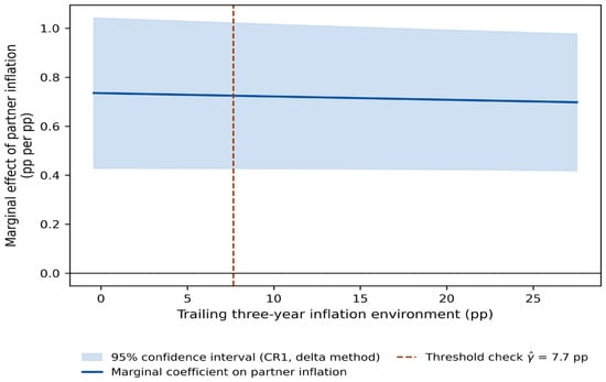
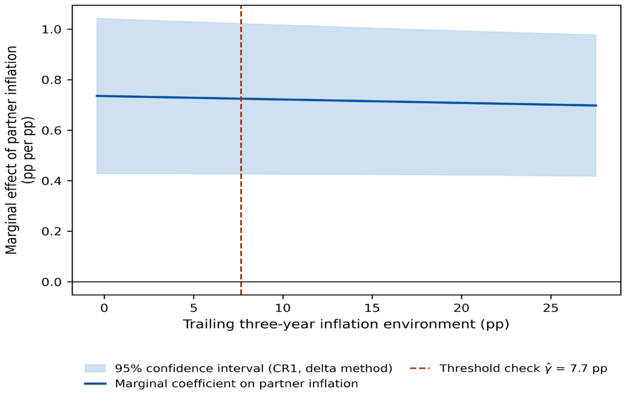
H4, the Taylor-type prediction that external-price transmission strengthens in high-inflation environments, is tested here on a panel wide enough to do so. The pre-committed test interacts partner inflation with the trailing three-year mean of own inflation (all three lags required; N = 1625). The interaction is −0.0014 with a CR1 p-value of 0.336 and a restricted wild-bootstrap p-value of 0.506. This is a null, and I report it plainly, because the prediction is standard: external-price transmission in this commodity-exporter panel is not measurably state-dependent in the inflation environment (95 percent CR1 interval [−0.0042, +0.0015]; minimum detectable effect 0.0039, a tightly bounded null). A pre-committed Hansen-type threshold check (Hansen, 1999) locates the sum-of-squared-residuals minimum at a trailing environment of 7.7 percentage points, with below/above partner-inflation slopes of 0.27 and 0.87 that are directionally consistent with H4. Under the frozen discipline, however, the continuous interaction answers the hypothesis and the threshold point estimate is not headlined; Figure 4 shows the implied marginal-coefficient profile. The headline θ2 is unchanged in the H4 model (−0.240, CR1 p < 0.001).
Figure 4.
State dependence of partner-inflation transmission. Marginal coefficient on partner inflation implied by the continuous-interaction model, as a function of the trailing three-year inflation environment; the shaded area is the 95% delta-method confidence interval under CR1 clustering, and the dashed vertical line marks the non-headlined Hansen-type threshold check ( = 7.7 pp). The interaction itself is null (restricted wild-bootstrap p = 0.506). Source: Author’s calculations.
7. Discussion
7.1. Interpreting the Pattern
Taken together, the estimates describe a channel-specific and, on inspection, episode-specific form of regime conditioning. Partner-price pass-through, the channel most often cited when pegs are said to import inflation, turns out to be the general condition of commodity exporters: strong, contemporaneous, and statistically indistinguishable across regimes. The exchange-rate channel is where the full panel shows a hard-peg differential, and Section 5.6 shows what that differential is: the inflation response to the January 1994 realignment of the CFA franc, observed simultaneously in the seven member economies whose 1994 observations enter the sample and are coded, correctly under the de facto rules, as hard-peg years. A parity change inside a hard peg is the case in which exchange-rate pass-through is expected to be fast and complete—the change is large, discrete, and not expected to reverse, so there is little reason for importers to absorb it in margins—and the distributed-lag estimates confirm the timing: contemporaneous under the peg, spread over a year outside it. The reading I had prepared for a general hard-peg differential, in which peggers experience a purer, unbuffered version of the anchor’s effective-rate cycle because the bilateral rate is fixed and the multilateral rate is inherited from the anchor’s cross-rates, not being offset by an independent interest-rate response (Shambaugh, 2004), and in which float-side associations are attenuated by the composition of shocks behind the exchange rate (Forbes et al., 2018, 2020), is not what the data identify. Outside the CFA zone, hard pegs show a differential of about −0.08 that is statistically null in the headline, distributed-lag, and country-slope views alike; the mechanism may operate, but this panel cannot detect it.
The temporal structure follows. The differential is concentrated before 2000 (a formal break; Section 5.5) because the realignment is, and it is absent after 2014. Its attenuation under the Shambaugh coding is a separate matter—that coding also treats the 1994 CFA years as peg years, and the attenuation is definitional widening of the peg group, as Section 5.5 shows—so the classification sensitivity and the episode concentration are two facts, not one. Because the panel’s H4 interaction is null, I do not press an inflation-environment mechanism; the sub-period pattern is reported as structure, and its interpretation is now simpler than I first allowed: one large realignment inside one hard-peg zone, in a decade of higher average inflation.
7.2. The Single-Regime Benchmark, Embedded
The comparison with the single-regime benchmark is now sharp. Within the six dollar-pegged GCC economies, Husain (2026) reports a contemporaneous partner-inflation association of about 0.46, rising to roughly 0.65 when the partner basket is re-weighted with country-specific, backward-looking trade shares, alongside a negative fiscal-stance association and a post-2014 weakening of the external channel. The wide panel places those numbers in context. A strong within-year partner-price association is what commodity exporters look like under any regime whatsoever: the panel-wide coefficient is about 0.8 with a null peg differential. The GCC’s imported-inflation configuration is therefore the norm of its class rather than a consequence of its peg, and while the wide θ1 interval (Section 5.6) means peg amplification of that channel cannot be tightly excluded, none is detected. The effective-exchange-rate channel, where the wide panel does show a hard-peg differential, is not a fingerprint the GCC shares: the differential is carried by the CFA franc zone (Section 5.6), and the USD-anchor cell of Table 7 (−0.160, p = 0.069) is descriptively the weaker of the two anchor cells. The fiscal-stance association generalizes only in part. On the wide panel it is null in level and in interaction, and the interaction stays null when CAF is replaced by the headline balance or when the sample is restricted to economies with better-fitting first stages (Section 5.6); on those restricted samples, however, the level association reappears (−0.096, p = 0.003, at the 0.05 threshold; −0.090, p = 0.009, at 0.10). I read this as suggestive only, under the multiplicity discipline of Section 5.5, but it is consistent with the negative GCC fiscal-stance association being visible wherever the commodity orthogonalization is informative, while a regime difference in it is not. Those benchmark numbers are cited from that study; I do not re-derive them here.
7.3. Policy Reading
Stated in associational terms, the results carry two messages for the recurring peg debate among commodity exporters. The first message is that regime choice offers no measurable insulation of the partner-price channel. Strong within-year transmission of partners’ inflation is the norm across arrangements; a float should not be expected to mute it, nor a peg to worsen it. The second is that the hard-peg differential in the exchange-rate channel should not be read as a general cost of pegging. In the full panel, one standard deviation of the peg group’s own effective-rate movement is associated with about 1.4 additional percentage points of inflation under hard pegs relative to other arrangements, or about 2.3 in total; but that figure is carried by the CFA franc zone and largely by the 1994 realignment, and outside the zone the differential is small and statistically null. The exposure the panel quantifies is therefore the inflation cost of a large parity change inside a hard peg—a cost that belongs in the peg’s cost–benefit ledger as the price of realignment, not as a running charge for the anchor’s cycle. Whether hard peggers bear a continuing exposure to the anchor’s effective-rate movements, as the trilemma logic suggests they should, is a question this panel cannot answer: it neither confirms nor excludes a differential of the size found outside the CFA zone.
7.4. Limitations
Six limitations deserve explicit acknowledgement. None, I will argue, overturns the estimand.
First, the regime contrasts are associations. Regime choice is endogenous to inflation history and institutions, and the contrast is identified mainly across economies: the within-switcher estimator of Section 5.3 carries the same sign but is statistically null (−0.076, p = 0.282, twelve clusters), and the cross-sectional differential is itself concentrated in the CFA franc zone (Section 5.6), outside which it is of the same small, null magnitude. The long-spell subsample and the anchor-by-year specification (Table 5) discipline the comparison, but selection on unobserved slope-relevant characteristics cannot be excluded—which is why no causal language is used anywhere in the paper.
Second, the 2020–2024 regime codes are Author-coded from the AREAER. Every coded cell carries a filed source note and, more decisively, the headline differential is concentrated in the pre-2014 decades, years wholly covered by the published classification, so the result cannot be an artifact of the extension.
Third, the hard-peg boundary is classification-dependent. The differential attenuates as the peg definition broadens (PEG12), softens to a null under the Shambaugh strict coding on the 1990–2018 overlap (−0.111, p = 0.205), and reverses sign under announced de jure status on the 2000–2022 overlap (+0.230, p < 0.001, against +0.091 for the frozen classification on identical rows). The sub-period structure helps interpret the pattern, but the caveat stands: the estimand is a de facto contrast, and the paper supports no statements about announced regimes.
Fourth, first-stage CAF uncertainty is propagated for γ1 via the two joint bootstrap designs of Section 4.2 but not into the PEG1 × CAF interaction; because the omission can only understate that interval, the pre-committed null reading of θ3 is conservative, and the checks with the headline balance and with better-fitting first stages (Section 5.6) point the same way.
Fifth, partner inflation is measured with error for reporters with thin bilateral trade coverage, and the effective-rate series backfills a smaller partner basket in the early 1990s (507 flagged country-years in the panel frame, of which 84 enter the estimation sample, all before 2000). The ex-GCC, fixed-weight, and no-cut partner variants and the no-splice dependent-variable variant leave the headline essentially unchanged, and the pre-2000 differential strengthens rather than weakens when the backfilled rows are removed (Section 5.6), which bounds the plausible influence of these choices.
Sixth, one candidate economy is excluded for lacking a commodity export-price index, and seven survivors enter the baseline only through the control-restoring sensitivities. Both facts are disclosed, and the restored-sample estimates (−0.210 and −0.204 across the two splice sets; −0.210 with parsimonious controls) match the baseline.
8. Conclusions
This paper has asked whether the exchange-rate regime conditions how external prices and fiscal stance reach inflation in commodity exporters—a comparative question that single-regime evidence, however careful, cannot answer. This paper brought to bear a pre-registered panel of commodity-dependent economies over 1990–2024 (71 pass the audit rule; 64 contribute estimation rows), estimated two-way fixed-effects regressions interacting a hard-peg indicator with partner inflation, effective-exchange-rate growth, and a commodity-orthogonal fiscal-stance residual, and conducted the entire exercise under a design frozen before estimation.
I draw three principal conclusions. First, trading-partner inflation passes through strongly everywhere, with no measurable regime difference, though that null is imprecisely bounded: the imported-inflation configuration documented for dollar peggers is the commodity-exporter norm. Second, the exchange-rate channel is where the full panel shows a hard-peg differential: appreciation is associated with disinflation about 0.21 percentage points per point more strongly under hard pegs, or about 1.4 additional percentage points per standard deviation of peg-group effective-rate movement, and the differential is robust across the baseline and 39 pre-committed variants. Targeted decompositions show what it is: a CFA franc zone regularity concentrated in the 1994 realignment. Outside the zone the differential is about −0.08 and statistically null, matching the within-switcher estimate and the distribution of country-specific slopes; its concentration before 2000 (a formal break; Section 5.5), its contemporaneous timing, and its regional and anchor sensitivities are facets of that one fact, and it is separately sensitive to the hard-peg boundary, attenuating under the Shambaugh coding and absent under both behavioral and announced codings after 2000. The finding is a period-, classification-, and zone-dependent empirical regularity, not a general structural feature of hard pegs. Third, the comparative fiscal channel and inflation-environment state dependence, both theoretically expected, are tightly bounded nulls under the pre-committed protocol; I report both with the same prominence as the positive finding, and I flag that the partner-price interaction is, by contrast, an imprecise null.
Two implications follow. For policy, regime choice buys no measurable insulation of the partner-price channel, and the exchange-rate exposure the panel quantifies is the inflation cost of a large realignment inside a hard peg rather than a running charge for the anchor’s cycle; whether such a running charge exists at the size found outside the CFA zone is not something this panel can establish. For method, the pre-commitment protocol did what it was designed to do, and the decompositions of Section 5.6 did what the protocol alone could not: a set of variants fixed in advance showed the differential to be stable across the pre-committed variants, and a targeted decomposition showed what it was. The two are complements, and I report both.
These findings raise questions this paper cannot settle. Would invoicing-currency composition—the sharpest discriminating variable the dominant-currency framework offers—account for how much of a realignment is passed through, and how fast? Is the small, statistically null differential found outside the CFA zone a real but modest hard-peg exposure that a larger panel, or a decomposition of effective-rate movements into anchor-inherited and residual components, could detect? And what does the de jure comparison signify, given that, in the recent window, announced peg status carries, if anything, an opposite-signed association? A structural account of pass-through under realignment inside hard-peg zones, and of the inherited anchor cycle outside them, is the natural sequel, and it is better asked now that the comparative facts are on the table.
Supplementary Materials
The following supporting information can be downloaded at: https://www.mdpi.com/article/10.3390/economies14100430/s1, File S1: Replication package (frozen-design document, code, and data workbook).
Funding
This research received no external funding.
Data Availability Statement
The dataset was assembled by the Author entirely from publicly accessible sources: the Ilzetzki–Reinhart–Rogoff de facto exchange-rate regime classification, extended by the Author for 2020–2024 from the IMF Annual Report on Exchange Arrangements and Exchange Restrictions (AREAER); the Shambaugh peg classification; the IMF World Economic Outlook, Commodity Terms of Trade, and International Trade in Goods by Partner Country databases; the World Bank World Development Indicators and historical income classifications; the Bruegel effective exchange rate database (Darvas, 2012; 16 July 2026 update); the Chinn–Ito financial openness index; the UNCTAD State of Commodity Dependence; and the United Nations Main Aggregates Database (sensitivity analyses only). The commodity-orthogonal cyclically adjusted fiscal stance was constructed by the Author as described in Section 3 and Appendix A.
Acknowledgments
Claude (Anthropic; Claude Opus 4.8, Claude Opus 5) was used to assist with manuscript editing, including checking language clarity and consistency. All content was reviewed, verified, and revised by the Author, who takes full responsibility for the integrity of the work.
Conflicts of Interest
The Author declares no conflicts of interest.
Appendix A. Construction and Audit Summary
This appendix summarizes the construction rules; the complete frozen-design document (21 binding construction decisions, the inference plan, the pre-committed robustness set, and a dated amendment log) is provided as Supplementary Materials (File S1). Sample rule: UNCTAD dependence ≥ 50% ∪ GCC (115 candidates); admission requires ≥ 20 usable years jointly non-missing on the five core variables, usability requiring IRR coarse ≤ 4 and |π| ≤ 50 pp, plus ≥ 25 first-stage observations; attrition 115 → 111 (regime coverage) → 73 (usable years) → 71 (first-stage rule); one further candidate is excluded for lacking a commodity price index. Partner inflation: bilateral import weights, trailing five-year backward windows, positive flows, aggregate counterparts removed by partner code, partner-years above 50 pp excluded with renormalization; ex-GCC, fixed-weight (2010–2019), and no-cut variants. Commodity prices: rolling-weight export index baseline; fixed and export-plus-import variants. Effective exchange rate: 170-partner basket with 65-partner backfill where consecutive years are unavailable (507 flagged country-years). Fiscal: WEO actuals only, fiscal-year labels mapped by leading year. CAF: per-country residual of the balance on current and lagged commodity export prices, levels, Newey–West (three-lag) first-stage covariances. Regime: published IRR annual to 2016; monthly modal-with-December-tiebreak 2017–2019 (89.7% agreement with published annual on 5214 overlap country-years); Author-coded AREAER extension 2020–2024 under fixed conventions with per-cell source notes and filed documents. Dependent variable: WDI CPI with a 50 pp screen and a flagged WEO splice for two GCC members’ pre-WDI years. Chinn–Ito 2024 carried from 2023, flagged. All sensitivities referenced in the text were pre-committed before estimation.
Appendix B. Commodity-Orthogonal Fiscal First Stages, Survivor Economies
Table A1 reports the country-by-country first stages behind the CAF measure for the 71 survivor economies under the baseline rolling-weight export index: the fiscal balance regressed on a constant and the current and lagged commodity export-price index in levels, with Newey–West (three-lag) standard errors. Every survivor satisfies the ≥25-observation eligibility rule by construction of the sample. The full table across all price-index variants and all candidate economies is provided in the Supplementary Materials (File S1).
Table A1.
CAF first stages by survivor economy (rolling-weight export index).
References
- Banerjee, A. K., Sensoy, A., Goodell, J. W., & Pradhan, H. K. (2026). Exchange rate pass-through, inflation, and energy prices: The role of central bank intervention and liquidity conditions. International Review of Finance, 26, e70067. [Google Scholar] [CrossRef] [Scilit]
- Barnett, S., & Ossowski, R. (2002). Operational aspects of fiscal policy in oil-producing countries (IMF Working Paper 02/177). International Monetary Fund. [Google Scholar]
- Bauer, M. D., & Swanson, E. T. (2023). A reassessment of monetary policy surprises and high-frequency identification. NBER Macroeconomics Annual, 37, 87–155. [Google Scholar] [CrossRef] [Scilit]
- Cagan, P. (1956). The monetary dynamics of hyperinflation. In M. Friedman (Ed.), Studies in the quantity theory of money (pp. 25–117). University of Chicago Press. [Google Scholar]
- Cameron, A. C., Gelbach, J. B., & Miller, D. L. (2008). Bootstrap-based improvements for inference with clustered errors. Review of Economics and Statistics, 90, 414–427. [Google Scholar] [CrossRef] [Scilit]
- Céspedes, L. F., & Velasco, A. (2014). Was this time different? Fiscal policy in commodity republics. Journal of Development Economics, 106, 92–106. [Google Scholar] [CrossRef] [Scilit]
- Chinn, M. D., & Ito, H. (2006). What matters for financial development? Capital controls, institutions, and interactions. Journal of Development Economics, 81, 163–192. [Google Scholar] [CrossRef] [Scilit]
- Choi, I. (2001). Unit root tests for panel data. Journal of International Money and Finance, 20, 249–272. [Google Scholar] [CrossRef] [Scilit]
- Choudhri, E. U., & Hakura, D. S. (2006). Exchange rate pass-through to domestic prices: Does the inflationary environment matter? Journal of International Money and Finance, 25, 614–639. [Google Scholar] [CrossRef] [Scilit]
- Clarke, D., Romano, J. P., & Wolf, M. (2020). The Romano–wolf multiple-hypothesis correction in stata. Stata Journal, 20, 812–843. [Google Scholar] [CrossRef] [Scilit]
- Darvas, Z. (2012). Real effective exchange rates for 178 countries: A new database (Bruegel Working Paper 2012/06). Bruegel. (Dataset update of 16 July 2026). [Google Scholar]
- Driscoll, J. C., & Kraay, A. C. (1998). Consistent covariance matrix estimation with spatially dependent panel data. Review of Economics and Statistics, 80, 549–560. [Google Scholar] [CrossRef] [Scilit]
- Drukker, D. M. (2003). Testing for serial correlation in linear panel-data models. Stata Journal, 3, 168–177. [Google Scholar] [CrossRef] [Scilit]
- Erbil, N. (2011). Is fiscal policy procyclical in developing oil-producing countries? (IMF Working Paper 11/171). International Monetary Fund. [Google Scholar]
- Forbes, K., Hjortsoe, I., & Nenova, T. (2018). The shocks matter: Improving our estimates of exchange rate pass-through. Journal of International Economics, 114, 255–275. [Google Scholar] [CrossRef] [Scilit]
- Forbes, K., Hjortsoe, I., & Nenova, T. (2020). International evidence on shock-dependent exchange rate pass-through. IMF Economic Review, 68, 721–763. [Google Scholar] [CrossRef] [Scilit]
- Ghosh, A. R., Gulde, A., & Wolf, H. C. (2002). Exchange rate regimes: Choices and consequences. MIT Press. [Google Scholar]
- Gopinath, G., Boz, E., Casas, C., Díez, F. J., Gourinchas, P.-O., & Plagborg-Møller, M. (2020). Dominant currency paradigm. American Economic Review, 110, 677–719. [Google Scholar] [CrossRef] [Scilit]
- Gruss, B., & Kebhaj, S. (2019). Commodity terms of trade: A new database (IMF Working Paper 19/21). International Monetary Fund. [Google Scholar]
- Ha, J., Stocker, M., & Yilmazkuday, H. (2020). Inflation and exchange rate pass-through. Journal of International Money and Finance, 105, 102187. [Google Scholar] [CrossRef] [Scilit]
- Hansen, B. E. (1999). Threshold effects in non-dynamic panels: Estimation, testing, and inference. Journal of Econometrics, 93, 345–368. [Google Scholar] [CrossRef] [Scilit]
- Husain, M. (2026). External inflation exposure and fiscal policy under the dollar peg: Evidence from GCC economies. Economies, 14, 308. [Google Scholar] [CrossRef] [Scilit]
- Ilzetzki, E., Reinhart, C. M., & Rogoff, K. S. (2019). Exchange arrangements entering the twenty-first century: Which anchor will hold? Quarterly Journal of Economics, 134, 599–646. [Google Scholar] [CrossRef] [Scilit]
- Ilzetzki, E., Reinhart, C. M., & Rogoff, K. S. (2022). Rethinking exchange rate regimes. In G. Gopinath, E. Helpman, & K. Rogoff (Eds.), Handbook of international economics (Vol. 6, pp. 91–145). Elsevier. [Google Scholar]
- Im, K. S., Pesaran, M. H., & Shin, Y. (2003). Testing for unit roots in heterogeneous panels. Journal of Econometrics, 115, 53–74. [Google Scholar] [CrossRef] [Scilit]
- Klein, M. W., & Shambaugh, J. C. (2010). Exchange rate regimes in the modern era. MIT Press. [Google Scholar]
- Levy-Yeyati, E., & Sturzenegger, F. (2005). Classifying exchange rate regimes: Deeds vs. words. European Economic Review, 49, 1603–1635. [Google Scholar] [CrossRef] [Scilit]
- Maddala, G. S., & Wu, S. (1999). A comparative study of unit root tests with panel data and a new simple test. Oxford Bulletin of Economics and Statistics, 61, 631–652. [Google Scholar] [CrossRef] [Scilit]
- Nickell, S. (1981). Biases in dynamic models with fixed effects. Econometrica, 49, 1417–1426. [Google Scholar] [CrossRef] [Scilit]
- Pesaran, M. H. (2021). General diagnostic tests for cross-sectional dependence in panels. Empirical Economics, 60, 13–50. [Google Scholar] [CrossRef] [Scilit]
- Reinhart, C. M., & Rogoff, K. S. (2004). The modern history of exchange rate arrangements: A reinterpretation. Quarterly Journal of Economics, 119, 1–48. [Google Scholar] [CrossRef] [Scilit]
- Romano, J. P., & Wolf, M. (2005). Stepwise multiple testing as formalized data snooping. Econometrica, 73, 1237–1282. [Google Scholar] [CrossRef] [Scilit]
- Roodman, D., Nielsen, M. Ø., MacKinnon, J. G., & Webb, M. D. (2019). Fast and wild: Bootstrap inference in stata using boottest. Stata Journal, 19, 4–60. [Google Scholar] [CrossRef] [Scilit]
- Shambaugh, J. C. (2004). The effect of fixed exchange rates on monetary policy. Quarterly Journal of Economics, 119, 301–352. [Google Scholar] [CrossRef] [Scilit]
- Taylor, J. B. (2000). Low inflation, pass-through, and the pricing power of firms. European Economic Review, 44, 1389–1408. [Google Scholar] [CrossRef] [Scilit]
- UNCTAD. (2025). The state of commodity dependence 2025 (UNCTAD/DITC/COM/2025/3). United Nations. [Google Scholar]
- Webb, M. D. (2023). Reworking wild bootstrap-based inference for clustered errors. Canadian Journal of Economics, 56, 839–858. [Google Scholar] [CrossRef] [Scilit]
- Wooldridge, J. M. (2010). Econometric analysis of cross section and panel data (2nd ed.). MIT Press. [Google Scholar]

Disclaimer/Publisher’s Note: The statements, opinions and data contained in all publications are solely those of the individual author(s) and contributor(s) and not of MDPI and/or the editor(s). MDPI and/or the editor(s) disclaim responsibility for any injury to people or property resulting from any ideas, methods, instructions or products referred to in the content. |
© 2026 by the author. Licensee MDPI, Basel, Switzerland. This article is an open access article distributed under the terms and conditions of the Creative Commons Attribution (CC BY) license.