


Abstract
The rapid expansion of the Internet of Medical Things (IoMT) and intelligent assistive technologies has intensified the need for resource-optimized cryptographic hardware to protect sensitive biometric data. Cryptographic hardware performance relies primarily on modular arithmetic operations, especially field multiplication. Although the binary extension field provides carry-less arithmetic ideal for battery-powered devices, standard general-purpose processors lack the dedicated hardware required to execute these operations efficiently. This paper proposes a novel multicore-based modular multiplication algorithm that bridges this gap by exploiting the parallel coordination fabric and high-bandwidth interconnects of modern embedded multicore systems. Central to this work is the Progressive Product Reduction (PPR) paradigm, which optimizes hardware efficiency by integrating the multiplication and field reduction phases into a unified process, thereby minimizing intermediate data storage and computational depth. We introduce and analyze two distinct architectural strategies—Progressive Product Reduction with Column Division (PPR-CD) and Progressive Product Reduction with Row Division (PPR-RD)—and establish rigorous mathematical models to estimate hardware area, critical path delay, and exact operational latency across various core configurations. Our performance evaluation demonstrates that the PPR-RD architecture achieves superior Area-Delay Product (ADP) and energy efficiency, providing a scalable framework for securing sensitive biometric data in next-generation assistive devices. This implementation ensures robust cryptographic protection for assistive devices while maintaining energy autonomy and computational resilience essential for sustaining consumer trust, advancing global health equity, and driving financial stability in future digital economies.
1. Introduction
The technological trajectory of the twenty-first century has been significantly altered by the integration of intelligent assistive devices into the daily lives of individuals with disabilities, offering unprecedented levels of autonomy and diagnostic precision. Modern assistive technology (AT) has evolved from simple mechanical aids to complex, interconnected systems such as neuroprosthetics, high-fidelity smart hearing aids, and wearable physiological monitors that function as integral nodes within the broader Internet of Medical Things (IoMT). This transformation sits at the intersection of UN Sustainable Development Goal 3 (SDG 3), which demands equitable health solutions, SDG 8, which promotes inclusive economic growth by empowering individuals with disabilities to actively participate in the modern workforce, and SDG 9, which fosters resilient, eco-efficient infrastructures through innovative technological advancements. As these devices increasingly rely on wireless protocols like Bluetooth Low Energy (BLE) and Wi-Fi to synchronize with smartphones or transmit sensitive biometric data to healthcare providers, they encounter a sophisticated landscape of cybersecurity threats [1,2,3]. The sensitivity of medical data—which often contains fifty percent more identifiable information than data in other commercial sectors—makes these devices high-priority targets for cybercriminals seeking to exploit vulnerabilities for data theft, ransomware, or even life-threatening interference with device functionality [4].
The resolution of these security challenges is fundamentally reliant on the implementation of robust cryptographic protocols, such as Elliptic Curve Cryptography (ECC) and the Advanced Encryption Standard (AES), which provide the necessary framework for data confidentiality, patient authentication, and firmware integrity [5]. However, the integration of such high-level security measures into assistive technology is severely constrained by the physical and operational realities of embedded medical hardware. These devices operate within stringent power budgets, possess limited silicon area, and, most critically, must adhere to ultra-low, deterministic latency requirements to maintain the efficacy of real-time control loops and audio processing [6,7,8]. Traditional software-based implementations of cryptographic primitives are frequently insufficient for these tasks, as they lack the computational throughput and energy efficiency required for long-term wearable use.
To address this critical gap, specialized hardware accelerators for modular multiplication—the core arithmetic operation in the crypographic algorithms—have become indispensable [9]. In ECC, modular multiplication serves as the fundamental building block for point addition and doubling, which together constitute the high-level scalar point multiplication required for secure key exchange and digital signatures. Similarly, AES utilizes finite field arithmetic for its nonlinear substitution and diffusion layers, where efficient multiplication ensures high-speed data encryption.
The implementation of efficient cryptography on assistive devices necessitates a deep understanding of finite field arithmetic, specifically the binary extension field GF. Unlike prime fields GF, where addition and multiplication produce carry chains that increase gate delay and power consumption, arithmetic in GF is carry-less: additions are XOR operations and multiplications avoid carry propagation. This property simplifies hardware design and lowers energy use, making GF especially suitable for battery-powered wearable devices [6,10].
The effectiveness of GF multiplications depends critically on the choice of base representation and the irreducible polynomial employed. While representations such as Normal (NB), Dual (DB), and Redundant Basis (RB) offer unique advantages [11], Polynomial Basis (PB) arithmetic stands out for hardware implementation due to its simplicity, reliability, and the elimination of basis conversion overhead [12,13,14]. Hardware efficiency is further influenced by the irreducible polynomial chosen; while trinomials and pentanomials are generally preferred for their lower complexity, All-One Polynomials (AOPs) remain a viable candidate for specialized multipliers [15,16].
Despite the clear mathematical advantages of GF, general-purpose multicore systems are fundamentally unsuitable for these operations because their ALU hardware is optimized for fixed-point or integer datatypes. In a standard processor, the adder is composed of a string of full-adders for integer addition, and the parallel multiplier is designed for integer products using carry-save arrays. Even modern microprocessors, such as the ATMEL family, are limited to simple logical operations that do not scale for high-security field sizes like or 409 [17,18]. In contrast, a dedicated cryptoprocessor or Trusted Platform Module (TPM) is designed to support operations across several fields, including GF, GF, and polynomial rings for post-quantum security [19]. These specialized systems employ matrices of XOR gates for GF additions and utilize hardware accelerators—often implemented as non-programmable systolic arrays—to achieve high concurrency within a low power budget.
Historically, the design of these cryptographic processors relied on ad hoc techniques that lacked the precision required for modern multi-core embedded architectures. Compared to these informal methods, formal design techniques allow the designer to strictly control the level of parallelism, inter-processor communication, and processor workload [20,21]. Earlier studies utilized dependence graphs to model the algorithm by considering dependencies between pairs of variables [21,22]. While these models provided a starting point, they were limited in their ability to fully explore hardware trade-offs. To bridge this gap, researchers have introduced diverse optimizations, such as error-detecting arrays [23], unified multiplication/squaring units [24], and Montgomery modular multipliers with local communications targeting resource-limited IoT and edge devices [25,26]. Furthermore, advanced techniques in nonlinear task scheduling and mapping have allowed for better control over word size and communication overhead in multipliers for trinomial primitive polynomials [27].
Building upon these formal foundations, modern multicore technology aims to further reduce power through parallelism; however, it introduces significant challenges in workload balancing and inter-processor communication (IPC). In real-time assistive devices, distributing massive cryptographic operands across multiple cores can lead to routing congestion and increased switching activity, draining vital battery reserves. Existing systolic designs frequently struggle with the communication-to-computation ratio, where the “reduction” phase requires substantial data shuffling between processors to manage feedback bits. This overhead can lead to non-deterministic latencies that disrupt sensitive medical control loops.
To overcome these architectural hurdles, this paper introduces a novel multicore-based modular multiplication algorithm designed to bridge the structural gap between finite field cryptographic operations and the parallel processing architectures of embedded multicore systems. By moving beyond traditional single-core accelerators, the proposed approach treats the multicore environment as a parallel coordination fabric to execute the Progressive Product Reduction (PPR) paradigm. This method optimizes hardware efficiency by integrating multiplication and field reduction into a single, unified process, which significantly reduces intermediate data storage and minimizes computational depth compared to standard “multiply-then-reduce” implementations.
There are many algorithms for polynomial multiplication including schoolbook multiplication, merged modular multiplication via progressive product reduction (PPR), merged modular multiplication via progressive multiplier reduction (PMR), Montgomery multiplication, Toom–Cook, and number-theoretic transform. Montgomery multiplication is effective only when the same multiplier is used more than once because of the need to transform multiplication data into and out of the Montgomery domain. Toom–Cook multiplication requires a system of linear equations of the same size as the polynomial order. Number-theoretic transform requires transforming our multiplication data out of the transform domain. Further the number of multiplications is equal to the order of the polynomials.
This research proposes an evaluation framework for two distinct architectural strategies: Progressive Product Reduction with Column Division (PPR-CD) and Progressive Product Reduction with Row Division (PPR-RD). Through simplified complexity modeling, the framework estimates silicon area, critical path delay, and clock cycles across various core configurations. It is important to note that these hardware and latency metrics rely on analytical modeling and architectural complexity analysis rather than empirical FPGA synthesis or ASIC post-layout implementation, which remains an avenue for future investigation. Within this analytical scope, a key finding is that the PPR-RD architecture demonstrates superior efficiency, as reflected by a decreasing Area-Delay Product (ADP) with higher core counts. Ultimately, these metrics provide valuable design guidelines to ensure that resource-constrained assistive devices remain energy-efficient and responsive to real-time demands.
The structure of this paper is as follows. Section 2 provides background to the concepts discussed in this work. Section 3 provides mathematical formulation for the PPR multiplication algorithms developed in this work. Section 4 develops the two proposed multicore PPR multiplication algorithms. Section 5 introduces the basic word-based PPR with column division algorithm (PPR-CD). Section 6 develops the proposed PPR with row division algorithm (PPR-RD). Section 7 discusses the different options considered for the implementation of proposed modular multiplication algorithms. Section 8 derives estimates of area and delay complexities of the hardware comprising the multicore system. It also estimates the number of CPU clock cycles required to complete the Multiply-then-Reduce (MtR), PPR-CD and PPR-RD algorithms. Section 9 shows performance of the proposed designs in terms of area, delay, area-delay product, and estimated consumed energy. Section 10 provides summary of findings and concluding remarks.
2. Polynomial Reduction Overview
In this section, we present a concise review of polynomial reduction in GF. Assume, the field GF is constructed using a primitive trinomial , typically expressed as:
where typically .
To transform a polynomial of degree m into a valid element of GF, we must perform a reduction process. This operation ensures the resulting polynomial remains within the field’s defined degree constraints. We can express in the form:
with 2).
We can achieve modular polynomial reduction by adding to the target polynomial:
The following reduction substitution remains feasible for our analysis:
Lemma 1 details a straightforward reduction method for polynomials where the degree a equals or exceeds m ().
Lemma 1.
Consider a single-term polynomial with a degree :
where the degree a satisfies , and the resulting polynomial possesses a degree less than m:
Executing the reduction of requires only a single step.
Proof.
We can partition into the following form:
We can apply Equation (3) to reduce the term as follows:
To achieve single-step reduction for , the maximum degree of the reduced polynomial must satisfy the following inequality:
This confirms the desired result. □
Lemma 2 demonstrates the single-step reduction of a polynomial with degree .
Lemma 2.
Consider a polynomial of degree a having the form:
where B denotes the number of terms in . Reduction of in one step is possible when:
Proof.
Substituting the result of Lemma 1, we can replace the term in Equation (6) with :
Given that has degree , the reduction of the above product is achievable in a single step if the degree of satisfies the following inequality:
or
□
3. Modular Multiplication Using Progressive Product Reduction (PPR) Technique
Let C and D represent two polynomials within the finite field GF, where C is the multiplier and D is the multiplicand.
The product of two polynomials can be formulated through the Progressive Product Reduction (PPR) method as follows:
In Equation (9), the multiplication process precedes the polynomial reduction. This sequence results in a polynomial of degree , necessitating a computationally intensive reduction phase. Conversely, Equation (10) integrates multiplication and reduction into a unified process, significantly enhancing operational efficiency.
The formulation in Equation (10) can be represented as the following iterative procedure:
Equation (11) defines the initialization of the iterative process, beginning at the maximum index . The subsequent shifting and reduction steps are executed via the iterations in Equation (12). Finally, Equation (13) terminates the iteration, yielding the fully reduced polynomial result.
By applying the reduction rule from Equation (3), the iterative transformation described in Equation (12) can be stated explicitly as:
where the degree of the resulting reduced multiplier remains below m.
Table 1 details the modular multiplication process, illustrating the generation of individual partial product terms across successive rows for a field size of .
Table 1.
Modular multiplication operation, with each row representing a partial product for the case when .
3.1. The PPR Variables
The iterative process defined in Equation (12) can be represented through a bitwise operational framework:
where the indices are constrained within the ranges and .
Equations (15)–(18) are characterized by the dual dependence indices i and j. These iterations define a two-dimensional convex hull .
The algorithm inputs consist of polynomials C and D and F denote the partial product. Figure 1 illustrates the dependence graph (DG) for these iterations at . This visualization assumes a degree-256 trinomial structured as:
Figure 1.
DG for PPR multiplication representing the iterations in Equations (16) and (17). Case when and .
Equations (16) and (17) govern the updates for the intermediate partial product bits . This process is visualized in Figure 1 via diagonal lines, with the reduction operation specifically highlighted by red lines.
The multiplier bits C are associated with index j, denoted by vertical lines, while the multiplicand bits D relate exclusively to index i, indicated by horizontal lines. The partial products, being dependent on both i and j, are represented by the diagonal trajectories within the graph.
3.2. Word Based Standard PPR Algorithm
We can express the coefficients of our multiplier and multiplicand polynomials C and D as K-bit words. The polynomials will have the form:
The product given by
The DG for the standard word-based PPR algorithm is illustrated in Figure 2. To facilitate processor-level operations, multiplier bits (C) are partitioned into K-bit words. Figure 2 specifically depicts the configuration for with a word size . The total count of multiplier words is determined by:
To ensure m is an integer multiple of K, the most significant bit side of m may be padded with zero words.
Figure 2.
DG for the standard PPR algorithm, illustrating the grouping of multiplier bits into K-bit words. The analysis is based on the parameters , , .
The word-based iterations defined in Equations (15)–(18) can be reformulated as word-level operations:
where .
4. Multicore PPR Algorithm Development
The computational tasks for the word-serial PPR algorithm in Figure 2 and Equations (24)–(28) is best performed via multicore embedded systems. We assume the embedded system has R cores and the structure of each core is shown in Figure 3.
Figure 3.
Structure of a core in the PPR multicore system implementation.
Each core is composed of a CPU, shown in the upper part which contains an ALU and fast access cache. Each core also contains a hardware accelerator for specialized algorithms such as PPR algorithm implementation on a systolic array. A local memory block is also added and this can be accessed by other cores via a uniform memory access mode (UMA).
Based on Equation (25), the iteration index i serves as the primary scheduling trigger for the accelerator. In this context, the accelerator system is responsible for determining:
- Dividing the total number of iteration operations among the available R cores to ensure balanced computational load.
- Allocating a specific time value (or clock cycle) to the different iterations to maintain the data dependencies inherent in the bit-serial or word-serial process.
- Allocating a specific accelerator core to iteration i, determining which physical hardware resource executes each step of the reduction.
The following two subsections introduce two distinct multicore design strategies for optimizing the PPR algorithm. These options focus on how the workload is partitioned across the R cores to maximize throughput and minimize latency.
5. Multicore PPR with Column Division (PPR-CD)
In the first proposed design, the Q partial product and multiplier words are distributed across the available processing cores. Each core is assigned a specific segment of the multiplier to process. The number of words allocated to each core, denoted as Z, is calculated as:
where Q is defined in Equation (23). To ensure that the total number of words Q is an integer multiple of the number of available cores R, the multiplier is padded with zero words on the most significant word side as needed.
Partial product word is assigned to processor core r according to the following mapping relation:
Table 2 details the distribution of multiplier and partial product words among the cores for a configuration where , , , , and . In this setup, the 32 total words () are divided evenly among the 4 cores (), resulting in each core handling exactly 8 words (). The allocation is summarized in Table 2.
Table 2.
PPR-CD algorithm assignment of multiplier or partial product words , to the cores. Case when , , , and .
The partitioning of the DG into columns reveals that the work is not isolated within each core. The black and red arrows crossing the boundaries between cores represent the flow of partial product bits and reduction signals, respectively. This is provided via neighbour-to-neighbour bit exchange among the cores and a global shared bus.
Consequently, the global recurrence is localized. Each core r executes its assigned iterations by updating its specific partial product words (where ). The word-wise update for core r during iteration i is formulated as:
Equation (31) represents the initialization step which begins for the index value . Equation (32) represents the iterations for decreasing values of the index i starting at and ending at . Equation (33) represents the termination step where the outputs of the cores are aggregated.
In this parallelized architecture, the operation denotes the concatenation of words to maintain the integrity of the bitstream across word boundaries.
The proposed multi-core architectures optimize inter-core communication to eliminate complex routing overhead. Specifically, as illustrated in Figure 2, the PPR-CD design features no communication between the cores during execution, as only the rightmost processor broadcasts the reduction terms of the shifted polynomial from the previous iteration. This broadcast data avoids access conflicts since only a single source of information is needed per iteration, and no data aggregation is required at the end of the iterations because each core directly produces the final result without communicating with the other processors.
The algorithm is structured into three distinct functional phases that execute across the multicore fabric. The following equations define the life cycle of the multiplication within each core:
- Equation (31) (Initialization): Each core r prepares its local registers and loads the assigned Z words of the multiplier.
- Equation (32) (Core Iteration): This is the high-performance phase where all cores update their partial product words concurrently.
- Equation (33) (Termination): Once all m iterations are complete, the cores stop, and the final reduced product is gathered from the distributed word registers.
It is important to emphasize that the operations defined in Equations (31)–(33) are executed simultaneously by all R cores.
6. Multicore PPR with Row Division (PPR-RD)
This proposed design is based on the result of Lemma 2. The system operates on data indexed by iteration i. The three primary data types—multiplier words , partial product words , and multiplicand bits —are partitioned into N groups. Each group is then assigned to a specific core r according to the following mapping relation:
If m is not an integer multiple of R, then we augment m with extra bits to make it so.
To ensure that the total number of iterations m is an integer multiple of the number of available cores R, the multiplicand D can be padded with zeros on the most significant bit side.
To assign bit with index i to a core and to determine the timing of the operations involving , we perform the following division operation:
In this approach, we define s as the quotient and r as the remainder resulting from the division of index i by the number of cores R. The bounds on these values are:
By substituting the division parameters into the index i, the multiplicand bit is transformed into a double-indexed variable . This notation specifies both the temporal stage s and the core r for each bit:
The relationship between the bit index i, the local iteration s, and the core index r is governed by Equation (35). The symbol indicates that the multiplicand bit is mapped to core r and is processed during local iteration s. Table 3 demonstrates this allocation for the case where bits are distributed across cores, resulting in local iterations per core.
Table 3.
Allocation of multiplicand bits to the cores in the PPR-RD algorithm for the case when , , and .
To implement the PPR-RD algorithm effectively in a multicore environment, we pivot from a global iteration index i to a dual-coordinate system defined by the quotient s and remainder r. This modification allows us to re-examine the shifted partial product from Equation (10) through a parallel processing framework. By applying the indexing relationship from Equation (35), the term is reformulated as:
Building on the double-indexing approach, the iterations originally described in Equations (11)–(13) are restructured to accommodate the parallel processing of multiple bits. This modification transforms the sequential algorithm into a concurrent multicore execution model.
where and .
It is important to highlight that the initialization operations defined in Equation (39) consist of R distinct terms that can be processed simultaneously. Specifically, the initialization term is assigned to and computed by accelerator core r. In this context, the remainder r serves as a spatial identifier, designating exactly which physical core is responsible for that specific portion of the calculation. Furthermore, the quotient s used in Equation (40) governs the temporal execution of the algorithm. Since this value is evaluated during each local cycle, the quotient s indicates the specific point in time that the operations corresponding to index i are performed.
Table 3 illustrates that each core deals with select bits of the multiplicand bits but each core deals with all the words of the multiplier. Within each core, each partial product word is shifted to the next higher-order position, which corresponds to a shift of bit positions to the left, prior to advancing to the subsequent row. The most significant word in each row represents the polynomial as defined in Lemma 2. From Table 3, these specific words are identified as rectangles with red boundaries, while the red arrows located on the right of each row signify the constant shift factor of . A significant advantage of this configuration is the dramatic reduction in computational depth. By utilizing cores, the number of rows that each individual core must process is reduced from the total bit length of down to just iterations. This design demonstrates that as the number of cores is increased, the workload per processor is proportionally diminished. This scalability offers a clear performance improvement over the traditional systolic implementations of the PPR algorithm found in the existing literature, such as [10,26,27]. Furthermore, the updated iterations in Equation (40) reflect a fundamental change in the algorithm’s operational logic. The multiplier shift value has been transformed into instead of the standard x. This shift to allows the system to maintain alignment across the parallel fabric, ensuring that the feedback and accumulation processes remain mathematically consistent even as multiple bits are processed during a single clock cycle.
6.1. Proposed PPR-RD: Algorithm Phases
The multicore approach to modular multiplication is organized into a three-part workflow, derived from the mathematical foundations of Equations (39)–(41):
- Setup Phase: This initial step handles preparatory tasks and is designed for concurrent distribution across multiple processing units.
- Recursive Phase: This primary segment performs the main computational cycles, leveraging accelerator cores to process data simultaneously.
- Finalization Phase: This concluding step is naturally successive, requiring a single-threaded process to resolve the ultimate result.
The proposed PPR-RD multi-core design optimizes inter-core communication throughout the execution of each iteration, ensuring that each processor stores its local intermediate data independently for the subsequent cycle. Upon completion of the iterative process, the R constituent cores must accumulate their distributed results to yield the final output. To accomplish this efficiently without bus contention or routing bottlenecks, a single core is designated to perform the accumulation, while the remaining cores communicate their results sequentially to this selected core in a conflict-free manner.
6.1.1. PPR-RD Setup Phase
Each core independently executes its specific version of the shifted partial product . To facilitate this, the setup phase follows these steps:
- Multiplier Broadcast: The I/O interface transmits the multiplier C to all accelerator cores simultaneously.
- Initial Local Calculation: Each accelerator core r computes its specific version of the initial shifted partial product.
In this framework, the variable r serves as a dedicated identifier for the r-th accelerator core.
The procedure for the setup phase is detailed in Algorithm 1, which outlines the specific operations executed during the start-up sequence. In this process, we perform a parallel startup by initializing R separate versions of the partial product, specifically .
| Algorithm 1 PPR-RD Setup Phase |
| 1. PARALLEL FOR DO 2. 3. END PARALLEL FOR |
6.1.2. PPR-RD Recursive Phase
In the recursive phase, the individual operations from Equation (12) are expanded into R simultaneous processes acting on distinct partial product segments, as detailed in Algorithm 2. Every core functions in parallel to execute the specific logic defined in Equation (40), with the fundamental distinction that the shift factor is now escalated to rather than the traditional x.
The algorithm effectively partitions the m rows shown in Figure 1 into R separate blocks, where each block contains rows. To ensure that m is perfectly divisible by the core count R, supplementary rows are appended at the bottom, and the most significant bits of multiplicand D are padded with zeros for alignment. The specific procedures for this phase are formalized in Algorithm 2, which illustrates the iteration cycles of the proposed multicore PPR accelerator. By distributing the m rows into localized blocks of N rows, the system achieves a significant reduction in serial processing time.
In Line 3 of Algorithm 2, the modular reduction process utilizes the R most significant bits of the partial product . This ensures that the parallel feedback logic remains mathematically equivalent to the sequential version while accounting for the larger shift factor. The PARALLEL FOR loop, encompassing Lines 1 through 5 of Algorithm 2, is executed concurrently. Each individual branch of this loop is assigned to a specific accelerator core, allowing all R cores to process their respective data segments at the same time.
| Algorithm 2 PPR-RD Recursive Phase |
| 1. PARALLEL FOR DO 2. FOR DO 3. 4. END FOR 5. END PARALLEL FOR |
6.1.3. PPR-RD Finalization Phase
The finalization phase is strictly serial and is responsible for generating the definitive modular product F. During this stage, a designated accelerator core is assigned the task of assembling the final result. This lead core communicates with all other accelerator cores to retrieve their respective partial products, . The final product is then calculated as follows:
The procedures for this final stage are summarized in Algorithm 3. This algorithmic description details the sequential logic required to aggregate the distributed results from each core into the definitive modular product.
| Algorithm 3 PPR-RD Finalization Phase |
| 1. ; 2. FOR DO 3. 4. END FOR |
7. Approaches to Implement Modular Multiplication Algorithms
The subsequent subsections examine four primary architectures for executing modular multiplication within the GF field:
- Multiply-then-reduce (MtR): Detailed in Section 7.1.
- Standard Progressive Product Reduction (PPR): Detailed in Section 7.2.
- Multicore PPR with Column Division (PPR-CD): Detailed in Section 7.3.
- Multicore PPR with Row Division (PPR-RD): Detailed in Section 7.6.
The analysis provided in these sections assumes the availability of a processor architecture specifically designed to support the respective algorithm under discussion.
7.1. MtR Processor Architecture
The Multiply-then-Reduce (MtR) strategy executes polynomial multiplication on two m-term polynomials. The coefficients of the multiplier polynomial C are expressed as K-bit words while the coefficients of the multiplicand polynomial D are expressed as bits:
The product given by
This product is equivalent to the convolution operation expressed in the form
Figure 4 illustrates the dependence graph corresponding to Equation (47) for the case , and .
Figure 4.
DG of MtR polynomial multiplier. Case , , and .
The figure indicates that the MtR algorithm requires multiply/add operations. To maintain data integrity and prevent resource contention, the timing of the blocks must be carefully synchronized. This ensures that only one multiplier word and one multiplicand word are delivered to a specific block at any given time.
We notice from the dependence graph that each product term is the addition of several partial products that lie on the same diagonal line as indicated. Since the addition operation is commutative, we can write the following iterations to evaluate the product terms:
The architectural layout of the processor designed for the MtR algorithm is illustrated in Figure 5. The ALU is divided into three specialized modules to handle the distinct phases of the operation, supported by a dual-bank register system for efficient data flow. To handle the specific data requirements of the partitioned multiplier, the processor utilizes specialized hardware for bit-shifting and final reduction via the LFSR.
Figure 5.
The processor’s hardware organization for implementing MtR algorithm.
- ALU Modules
- The Selector Module: This unit acts as the primary data interface and functions as the traffic controller for the K-bit words entering the ALU. The selector performs a bit-slicing operation where a single input word is used to generate two distinct output words, and . This ensures that the multiplier and multiplicand components are correctly aligned with the multiplier’s internal grid. The logic for generating these outputs is governed by the following expressions:
- The Multiply-Add Module: This is the core computational engine that executes the polynomial multiplication while integrating high-speed multiplication with field-specific addition. It consists of two primary hardware components designed for GF arithmetic: a multiplier and a K-bit GF adder. The multiplier layer consists of an array of AND and XOR gates to produce the partial products. Complementing this is the adder unit, which is simplified into K parallel, two-input XOR gates. Since there is no carry propagation in this field, the addition is strictly bitwise, allowing for very low operational latency during the accumulation of partial products.
- The Linear Feedback Shift Register (LFSR) Module: Once the full product polynomial F is generated, this module performs the modular reduction phase, reducing the -bit product F via a Galois LFSR configuration. This setup uses feedback taps corresponding to the field polynomial to “fold” the result back into GF. This specific configuration is often preferred in hardware because the XOR gates are placed directly between the flip-flops, which significantly minimizes the critical path delay compared to other architectures.
- Register BanksThe MtR processor maintains two sets of register banks to manage inputs and intermediate results:
- Input Banks (C and D): Located at the top left, these two banks each contain Q registers of K-bits. They store the words of the multiplier C and the multiplicand D, feeding them into the selector as needed.
- Product Banks ( and ): Located at the top right, these two banks also contain Q registers of K-bits each. They are responsible for storing the intermediate product results from the top-bottom () and left-right () paths, eventually holding the final product before reduction.
7.2. Basic PPR Algorithm Implementation
Figure 6 illustrates the processor architecture designed to execute the word-based PPR algorithm, adhering to the data flow in Figure 2 and the iterative sequence from Equations (24)–(28). The system relies on the selector module to route data into the multiply-add module. The multiply-add module is structurally organized into parallel data paths to independently process multiplication and addition operations through sequential stages of registration, logic evaluation, and output multiplexing. In the multiplication pathway, the polynomial multiplier concurrently processes the operands using a parallel array of bit-multiplier blocks, each constructed from a two-input NAND gate followed by an inverter to execute optimized AND logic, before the accumulated partial products are latched into the intermediate product register. Simultaneously, the addition pathway evaluates the operands using an array of parallel, two-input XOR gates to perform strictly carry-less, bitwise GF additions in a single clock cycle, storing the resulting sum in a separate intermediate register. Finally, an output multiplexer interfaces with both intermediate registers, driving the appropriate computed result onto the primary output bus under deterministic scheduling control.
Figure 6.
Word-Based PPR Algorithm Processor Architecture.
The PPR processor manages data through three distinct register banks:
- Multiplier and Multiplicand Banks: Two K-bit banks, each containing Q registers, dedicated to storing polynomials C and D.
- Product Bank: A single K-bit bank F with Q registers used to store both intermediate partial products and the final modular result.
7.3. Multi-Core Architecture of PPR-CD Option
The distribution of the multiplier bits within the multicore framework is illustrated in Table 2, while the physical architecture of the PPR-CD implementation is detailed in Figure 7. This system achieves parallelization by partitioning the data across multiple processing units to handle large-scale GF operations. A key feature of this design is that each core is responsible for only a subset of the total multiplication task: it operates exclusively on Z multiplier words and the corresponding partial product words. However, to complete its local calculations, every core must have access to all the multiplicand bits. Specifically, Core r utilizes:
Figure 7.
PPR-CD algorithm implementation: each core handles Z multiplier and partial product columns and entire multiplicand bits.
- Z contiguous words of the multiplier and the partial product registers.
- All the multiplicand bits, which are broadcast to every core in the system.
Notice that the cores communicate together through neighbour-to-neighbour communication and a broadcast bus. Each core accepts input bits from its left neighbour and the broadcast bus. Only the processor on the right broadcasts the reduction bit to all the cores.
Implementing the PPR-CD algorithm on this multicore hardware requires two primary coordination tasks. First, the projection of words must be performed to assign the specific data segments as discussed in Section 7.4. Second, the workload scheduling for each core must be managed as discussed in Section 7.5.
7.4. Projection Function Construction for PPR-CD Algorithm
In the PPR-CD design, and represent the multiplier and partial product words for any given column j, where the index j spans from 0 to . To organize the data across the system, a projection function is employed. This function allocates every multiplier word and partial product word within columns to a specific processing core, adhering to the mapping criteria established in Equation (30).
7.5. Scheduling Function Construction for PPR-CD Algorithm
The selection of the scheduling function is governed by the projection function established in Equation (30). Several critical requirements must be met during this process:
- Concurrent Row Processing: All cores responsible for the Q words within a specific row function in parallel.
- Defined Workload: Each individual core handles Z words, where the quantity Z is derived from Equation (29).
The specific timing value assigned to the execution of partial product words at iteration i and column j is formulated as follows:
Table 4 presents the execution schedule for the multicore PPR-CD implementation, specifically focusing on the initial Z columns. This example is configured with the parameters , , , , and .
Table 4.
Execution Timeline for Multicore PPR-CD Algorithm Configuration: Case when , , , , .
7.6. Multi-Core Architecture of PPR-RD Option
The assignment of multiplicand bits across the various cores is detailed in Table 3, where each individual core is responsible for processing a segment of N multiplicand bits. The hardware configuration for this multicore PPR-RD implementation is depicted in Figure 8. In this specific setup, Core r is equipped with the following data components:
Figure 8.
PPR-RD algorithm implementation: Each core processes all multiplier words and N multiplicand bits.
- Multiplier Access: It utilizes every word of the multiplier C.
- Initial State: It receives the initial shifted partial product from the preceding iteration, represented as .
- Partial Product Mapping: The specific partial product words are allocated to the core based on the mathematical mapping defined in Equation (35).
- Multiplicand Rows: It operates on N specific multiplicand rows, ranging from to , as previously organized in Table 3.
Mapping the PPR-RD algorithm tasks to the different cores is discussed in Section 7.7. Scheduling the PPR-RD algorithm tasks is discussed in Section 7.8.
Earlier research by authors in [21,27,28] focused on the development of specialized accelerators specifically engineered to implement the PPR algorithm efficiently. Their primary motivations were the optimization of algorithm latency and the precise control of processor workloads through dedicated hardware. In contrast, the current objective is to map the PPR algorithm onto an embedded multicore system containing R cores. This shift in platform significantly influences the design of the timing and projection functions. Given the priority of integrating the algorithm into this embedded multicore environment, the design process commences with the projection function.
7.7. Projection Function Construction for PPR-RD Algorithm
In the PPR-RD implementation, we represent the multiplier and partial product words at a specific iteration i and column j as and . The indices for these elements range such that and . To distribute the workload across the hardware, these words are assigned to a specific core, denoted as core r, following the mathematical mapping defined in Equation (35). Table 5 provides a practical example of this distribution for an embedded multicore system. This specific mapping illustrates how the partial product words are allocated when the system is configured with columns and cores.
Table 5.
Distribution of Partial Product Words Across Processor Cores. Case when , .
This mapping strategy distributes the partial product words across the multicore system, where each individual core is responsible for a specific quantity of words, denoted as N. The value of N is formally defined in Equation (34). As illustrated in the mapping table for the and configuration, Core manages 8 specific partial product words. These words are assigned using an interleaved pattern: and . This arrangement ensures that the total computational load of the partial products is partitioned into manageable segments for each processing element in the embedded system.
7.8. Scheduling Function Construction for PPR-RD Algorithm
The scheduling function is responsible for transforming the dependence graph into a directed acyclic graph (). In [28], the authors employed a formal design methodology to identify all feasible scheduling functions for the PPR algorithm. Their research highlighted two specific functions, one of which provides system designers with the ability to regulate the count of systolic processing elements and the specific workload assigned to each processor. The assignment of multiplier and partial product words to cores, as well as the timing of the update equations for each iteration, is governed by Equation (35). This function is designed to meet two primary operational requirements:
- Word Processing: Every individual core is responsible for processing all words within a specific row.
- Parallel Execution: All cores function simultaneously, each operating on a different row.
For the multiplier and partial product words and , the associated timing function is defined as:
8. Performance Complexity Evaluation of Modular Multiplication Algorithms
In this section, we analyze the performance complexity of the four modular multiplication algorithms examined in this study. Prior to hardware complexity modeling, the functional correctness of the proposed architectures was validated using a bit-accurate software model developed in MATLAB (Version 24.2, R2024b), ensuring correct finite field arithmetic across all examined core configurations (R). Building upon this verified logic, the evaluation begins with a review of the area and delay complexities associated with the fundamental gates and modules. These components serve as the primary building blocks for the hardware implementations. By establishing these baseline metrics for the basic hardware elements, we can accurately assess the overall efficiency and physical resource requirements of each multiplication architecture. Nevertheless, it is important to note that these evaluations rely on analytical estimations and structural complexity proxies, such as normalized area and delay. While these analytical metrics effectively characterize relative scaling trends across varying core counts (R), absolute figures for maximum operating frequency, resource utilization (such as look-up tables and flip-flops), and post-synthesis dynamic or static power require physical implementation on target FPGA or standard-cell technologies, which remains an important avenue for future work.
The order of the primitive polynomials m is varied in this work over the range 100–1000. A primitive polynomial or degree m is found using the following approach. The root is obtained with the following order [29,30,31,32]:
The number N of primitive polynomials of degree m is given by
where is Euler’s totient function and N is always a positive integer. We should bear in mind that the primitive polynomials could have any coefficient distribution and is not confined to trinomials or pentanomials. Regardless of the type of primitive polynomial, we can always express it in the form:
where .
A reduction operation allows us to write
and we can always write
Therefore, the reduction operation simply adds polynomial , when needed, at each iteration in Algorithm 2.
8.1. Modeling Area and Delay Complexity at the Gate Level
This section provides a comparative analysis of the delay, area, and area-delay product (ADP) required to execute the various modular multiplication implementations. The discussion opens with a concise summary of power consumption sources within a CMOS integrated circuit. We aim to establish a relationship between this power usage and the physical chip area. Furthermore, we argue that the area × delay product (ADP) serves as an equivalent metric for the total energy consumption of the integrated circuit.
8.2. Contributors to Power Consumption in an Embedded Systems
Embedded systems experience power dissipation across multiple operational scales. At the global level, power loss stems from memory access operations, interconnect ohmic and parasitic capacitances, leakage currents in idle components, and clock tree distribution overhead. Notably, the clock distribution tree represents the longest switching transmission line within an integrated circuit. At the local level, gate parasitic capacitance switching, transistor leakage and overlap power loss in CMOS technology. Developing a model for all these power loss mechanisms is beyond the scope of this work and requires dedicated work to be inclusive. We will confine our discussion here to power loss at the gate level and argue that the other global power loss mechanisms are always present in a comparable scale for the different models discussed here.
In CMOS technology, power consumption primarily originates from three distinct sources: static leakage, dynamic switching, and the overlap current that occurs when transitioning between logic states. Understanding these components is essential for evaluating the hardware efficiency of our modular multiplication implementations.
Static leakage is fundamentally linked to the semiconductor junctions formed by the transistor’s source and drain areas. Because these physical dimensions define the junction, we can assume that leakage power consumption is directly proportional to the total gate area. This relationship allows us to use area complexity as a proxy for the static power requirements of the four algorithms under study.
Dynamic switching power is defined by the expression , where P represents parasitic capacitance, f is the switching frequency, and is the supply voltage. Given a constant frequency and supply voltage across the system, the dynamic power depends entirely on the parasitic capacitance. Since this capacitance is a function of the transistor’s source and drain areas, dynamic power is also considered proportional to the gate area.
Overlap power consumption occurs during the brief period when a gate is in an intermediate state, neither fully 0 nor 1. The current flowing during this transition depends on the gate’s drive capacity, which is a function of gate width rather than total area. While this makes overlap power the only component independent of gate area, modern CAD tools and design methodologies focus heavily on minimizing it to prevent performance degradation.
Consequently, we focus our complexity analysis on static leakage and dynamic switching as the dominant power factors. Furthermore, the Area-Delay Product (ADP) is employed as a first-order hardware-efficiency and complexity proxy. Since active switched capacitance in synchronous CMOS scales proportionally with silicon area (), optimizing the ADP effectively bounds the theoretical energy-delay trade-off per operational cycle. This metric reliably serves as an architectural figure of merit given the streamlined, conflict-free communication structures of the proposed multi-core designs, where inter-core data distribution and final reduction aggregation are handled efficiently without complex multi-hop interconnection routing overhead.
8.3. Area and Delay Normalization Using a Base Inverter Reference
During system operation, all logic gates and hardware components share identical frequency (f) and supply voltage () parameters. This uniformity means that power performance is predominantly governed by the parasitic capacitance (P) of the circuit. Because the magnitude of this capacitance is a physical consequence of the transistor’s dimensions, the total hardware area acts as a direct surrogate for power consumption. Therefore, it is reasonable to conclude that area estimates are proportional to the power required by the implementation.
The delay and area performance parameters for the gates and circuits fundamental to finite field arithmetic hardware are summarized in Table 6. To provide a consistent comparison, the area is normalized against a minimum-area nMOS transistor, while the delay is normalized relative to a minimum-area inverter. The edge-triggered D-type flip-flop utilized in this study is based on a NAND gate configuration as detailed in [33]. Furthermore, all design selections for minimum-delay gates adhere to established VLSI design principles, such as those documented in [34]. These normalized metrics establish the necessary baseline for calculating the overall complexity of the modular multiplication algorithms.
Table 6.
Normalized gate-level characterization (propagation delay and equivalent area) for binary extension field arithmetic primitives.
To accurately determine the delay across various designs, we must first estimate the total number of clock cycles required to execute the computational steps of each modular multiplication algorithm. To achieve this, we establish a set of standard register transfer level (RTL) instructions tailored to the specific hardware configurations under study. By defining these basic instructions, we can map the high-level algorithmic logic onto the physical hardware clock cycles, providing a clear path for calculating the total execution time.
To demonstrate the application of these RTL instructions, we examine the basic multiply-add module of the hardware multipliers. In this configuration, the multiplier generates a full product split into two distinct K-bit results: the Least Significant Word (LSW) and the Most Significant Word (MSW). The specific sequence of RTL steps required to manage these outputs and execute the operation is detailed in Figure 9. This example serves to bridge the gap between abstract algorithmic steps and the physical movement of data between registers during a multiplication cycle.
Figure 9.
RTL Implementation: Loading Registers R1, R2, Multiplying, and Storing Results to R3 (LSW), R4 (MSW).
Based on the sequence provided, the multiply-add operation requires a total of 5 clock cycles to complete. During this interval, the hardware executes the necessary RTL instructions to process the inputs and stabilize the results for both the Least Significant Word (LSW) and the Most Significant Word (MSW). This 5-cycle duration establishes the baseline timing for a single multiplication step, which is a critical factor when calculating the total delay of the modular multiplication algorithm as it scales across the multicore system.
8.4. Complexity Evaluation of the MtR Algorithm
As shown in Figure 5, the overall clock cycle duration (TC) is determined by the maximum propagation delay across three primary hardware modules (selector, multiplier-adder, and LFSR). By analyzing the internal architectures of the modules, it becomes evident that the multiplier-adder module exhibits the longest path . Consequently, the clock period is effectively governed by , leading to the following simplified expression:
The total clock cycle count for the multiplier-based MtR modular multiplication algorithm is evaluated by tracking its machine-level execution flow, where each instruction is processed within a single clock cycle. This architectural analysis yields the following execution cycle formula:
In this equation, the constant factor of 13 represents the overhead incurred by transferring operands from the register banks to functional units, such as the shifter and the CPU, during each iteration. Consequently, the total delay for the MtR algorithm is calculated by multiplying this cycle count by the clock period:
Drawing from the architectural layout in Figure 5, the total area of the MtR processor is determined by the sum of its constituent hardware modules:
Based on the architecture depicted in Figure 5, the total area of the MtR processor is calculated by summing the footprints of its primary functional modules, including the register banks (), the selector (), the multiplier-adder (), and the linear feedback shift register (). These individual areas are derived from their internal gate counts and storage elements, where the registers scale with the parameters Q and K, while the multiplier-adder logic is dominated by the quadratic complexity. The specific area expressions are:
To assess the overall design efficiency, we use the Area-Delay Product (ADP). This metric combines the total physical area () with the execution time () to provide a comprehensive measure of hardware performance:
8.5. Complexity Evaluation of the PPR Algorithm
Based on the architecture depicted in Figure 6, the clock cycle period () is governed by the maximum propagation delay between the selector and the multiplier-adder modules: An evaluation of the internal module topologies reveals that the critical path resides within the multiplier-adder unit, whose propagation latency strictly bounds the system performance compared to the selector block. Accordingly, the operational clock period of the PPR processor is explicitly determined by the worst-case gate-level delays accumulated along this specific pathway:
The total clock cycle count for the PPR modular multiplication algorithm is evaluated by tracking its machine-level execution flow, where each instruction is processed within a single clock cycle. This architectural analysis yields the following execution cycle formula:
By multiplying the clock period by the total cycle count, the overall execution time for the PPR algorithm is established as:
In alignment with the architecture shown in Figure 6, the area of the PPR processor is calculated by summing the areas of its primary hardware components:
where the terms are expressed as follows:
The overall hardware efficiency of the PPR implementation is quantified by the ADP. This metric is determined as:
8.6. Complexity Evaluation of the PPR-CD Algorithm
Because the internal structure of the PPR-CD processor is identical to the one shown in Figure 6, it inherits the same timing constraints. This means the clock frequency is limited by the critical path of the multiplier-adder unit, ensuring the clock period remains consistent with the standard PPR design. To determine the total runtime, we first find the clock cycle count, , which is derived by evaluating the maximum range of the loop indices within the PPR-CD algorithm:
Consequently, the total execution delay for the PPR-CD algorithm is calculated by multiplying the operational cycle count by the duration of a single clock cycle:
Based on the architecture illustrated in Figure 6, the physical area of the PPR-CD processor is estimated by summing the footprints of its primary hardware blocks along with additional logic required for this specific variant:
where the factor R on the RHS accounts for the total multicore area and terms are expressed as follows:
The estimated ADP performance for the PPR-CD algorithm is represented by:
8.7. Complexity Evaluation of the PPR-RD Algorithm
The internal processor architecture for the PPR-RD algorithm is similar to that depicted in Figure 6, with the clock period estimated using Equation (72). To ascertain the total number of clock cycles required for the completion of the PPR-RD algorithm, one must refer to the analysis of the machine-level instructions of the PPR-RD algorithm under uniform single-cycle execution. This analysis yields the following execution cycle formula:
Consequently, the overall delay of the PPR-RD algorithm can be expressed as:
Referring to Figure 6, the estimated area of the PPR-RD processor is calculated
where the definitions of the components are provided as follows:
The estimated ADP for executing the PPR-RD algorithm is expressed as:
9. Performance Results and Comparative Discussion
This section presents a comprehensive evaluation of the proposed multi-core architectures, analyzing key performance indicators including normalized area, delay, and Area-Delay Product (ADP). It examines how distributing workloads across multiple cores impacts overall execution efficiency and scalability trade-offs. It is worth noting that the estimated energy metrics and efficiency trends discussed throughout this section are inferred analytically from normalized ADP metrics and architectural complexity models rather than measured directly from physical FPGA or ASIC hardware implementations, serving as relative indicators of architectural efficiency.
9.1. PPR-CD Algorithm Performance Assessment
Figure 10 demonstrates a comparative analysis of the hardware resources required for the MtR, PPR, and PPR-CD modular multiplication algorithms. The figure shows that the normalized area for all architectures increases as the m scales from 100 to 1000 bits. Furthermore, the figure shows that the total area of the PPR-CD algorithm increases as the number of cores increases. The lowest area is that of the single-core PPR algorithm. In contrast, the multicore PPR-based architectures exhibit much higher area when the number of cores exceeds 2.
Figure 10.
Normalized area comparison for MtR, PPR, and PPR-CD algorithms. Parameters: –1000, , .
Figure 11 presents the normalized delay comparison for the MtR, PPR, and PPR-CD algorithms under the following test configuration: field size m ranging from 100 to 1000 bits, word width bits, and core count R taking values 2, 4, 6, and 8 cores.
Figure 11.
Normalized delay comparison for MtR, PPR, and PPR-CD algorithms. Parameters: –1000 bits, , .
The analysis of the Normalized Delay presented in Figure 11 highlights the significant performance gains achieved through the multicore architecture of the PPR-CD algorithm compared to traditional implementations. As the operand bit-length m scales from 100 to 1000, the MtR implementation consistently produces the largest normalized delay, representing the least efficient option for high-speed modular multiplication. While the standard PPR and the PPR-CD variant with cores show similar timing profiles, they both offer a considerable improvement over the MtR baseline. The performance of the PPR-CD implementations is characterized by unique stepped transitions, which are a direct result of the parameters Z and Q defined in the algorithmic timing equations. These steps reflect the discrete nature of word-based processing in the hardware.
The figure shows that the lowest four lines correspond to the multicore designs (), highlighting that the parallel operation of the cores significantly reduces execution time. Increasing the number of cores results in lower normalized delays, with PPR-CD 8 (the 8-core configuration) demonstrating the highest efficiency in the group. However, the data also reveals a trend of diminishing returns; the impact of adding more hardware resources becomes less significant for values of R higher than 8. This suggests that for the chosen word size of , cores represents an optimal balance between parallel speedup and hardware overhead.
Figure 12 illustrates the normalized ADP for the MtR, PPR, and PPR-CD algorithms, evaluated under the following parameters: field size m spanning 100 to 1000 bits, word width bits, and core count R set to 2, 4, 6, and 8. In general increasing the number of cores reduces the overall workload of each core and this results in reduced energy consumption.
Figure 12.
Normalized ADP (Estimated Energy Consumption) for MtR, PPR, and PPR-CD Algorithms. Parameters: –1000 bits, , .
The evaluation of the Normalized ADP provides a comprehensive look at the hardware efficiency of the various architectures. Because the ADP is derived from the multiplication of physical footprint and execution time, the resulting curves exhibit an exaggerated stepped pattern. This visual characteristic is a direct consequence of the cumulative influence of the individual stepped patterns observed in both the normalized area and the normalized delay curves, which are themselves dictated by the word-based parameters Z and Q. When comparing the different implementations, the MtR algorithm consistently shows the highest ADP values across the entire bit-length range ( to 1000), confirming it as the least cost-effective design. In contrast, the PPR-CD algorithm demonstrates significant optimization through its multicore approach. The data shows that increasing the number of cores for the PPR-CD algorithm results in progressively lower ADP values. Since hardware power is proportional to the silicon area, it can be concluded that the normalized energy (which is proportional to the normalized ADP) decreases almost directly as the number of cores increases. This indicates that the multicore PPR-CD architecture is not only the highest-performing option but also the most energy-efficient for large-scale modular multiplication tasks.
9.2. PPR-RD Algorithm Performance Assessment
Figure 13 depicts a normalized area comparison among the MtR and PPR algorithms. We notice that the least area is the single-core PPR algorithm. As expected, all multicore PPR-RD processors have larger areas. The 2-core PPR-RD processor and the MtR processor have approximately the same area.
Figure 13.
Normalized area comparison for MtR, PPR, and PPR-RD algorithms. Parameters: –1000, , .
Figure 14 shows the normalized delay for the MtR, PPR and PPR-RD algorithms. Case when m is in the range 100 to 1000, , and R has values 2, 4, 6 and 8 cores.
Figure 14.
Normalized delay comparison for MtR, PPR, and PPR-RD algorithms Parameters: –1000 bits, , .
The performance of the PPR-RD implementations shows stepped transitions due to the parameters Z and Q in Equations (29) and (23). For the chosen set of parameters, the figure shows that the MtR implementation produces the largest normalized delay compared to the PPR design options. The lowest four lines represent the normalized delays of the multicore designs. Due to parallel operations of the multicore designs the normalized delays are the lowest especially as the number of cores increases. We notice from the figure also that the effect of increasing the number of cores diminishes for values of R higher than 8.
Figure 15 presents the normalized ADP for the MtR, PPR, and PPR-RD algorithms, providing a comprehensive metric for architectural efficiency. The analysis spans operand bit-lengths (m) from 100 to 1000, utilizing a word size of and evaluating multicore configurations (R) of 2, 4, 6, and 8 cores. In general increasing the number of cores reduces the overall workload of each core and this results in reduced energy consumption. The ADP curves exhibit an exaggerated stepped pattern, resulting from the cumulative discrete transitions in both the normalized area and delay metrics. Across the entire range, the MtR implementation consistently yields the highest ADP values, identifying it as the least efficient architecture. In contrast, the PPR-RD algorithm demonstrates significantly enhanced efficiency as the number of cores (R) increases from 2 to 8. This reduction in ADP is particularly notable because the normalized area remains constant for all PPR-RD variants; thus, the performance gains are driven entirely by the reduction in computational delay through parallel processing. Furthermore, since hardware power is proportional to area, the normalized energy—which scales with the ADP—decreases almost directly as the core count increases, confirming the multicore PPR-RD architecture as a highly optimized and energy-efficient solution.
Figure 15.
Normalized ADP for MtR, PPR, and PPR-RD Algorithms. Parameters: –1000, , .
9.3. Comparative Performance Analysis: PPR-CD vs. PPR-RD Algorithms
The architectural efficiency of the PPR-CD and PPR-RD algorithms is evaluated across various multicore configurations ( and 8), as illustrated in Figure 16, Figure 17, Figure 18 and Figure 19. The results indicate that for all tested core counts, the PPR-RD implementation consistently achieves a lower ADP than the PPR-CD variant over the operand range of to 1000 bits. This consistent performance advantage demonstrates that the PPR-RD design maintains a more optimized balance between silicon area and execution speed. This high-performance balance carries significant weight for the operational stability of next-generation medical networks. In future digital health economies, where millions of IoMT nodes concurrently stream ledgered biometric records, architectural resource optimization directly scales down the computational footprints of edge servers. By lowering hardware resource dependencies without degrading processing speeds, the PPR-RD variant provides an economically scalable cryptographic solution that keeps consumer healthcare devices affordable, long-lasting, and highly accessible globally—directly fulfilling the foundational criteria of SDG 3 and SDG 9. Additionally, by ensuring these secure assistive devices remain reliable and accessible, this architecture supports SDG 8 targets by empowering individuals with disabilities to maintain productive, uninterrupted participation in the digital workforce. Furthermore, the data reveals a clear inverse relationship between parallelism and ADP; as the number of cores increases, the ADP values for both algorithms decrease significantly, reflecting the substantial throughput gains afforded by the multicore architecture.
Figure 16.
Normalized ADP for PPR-CD and PPR-RD algorithms ().
Figure 17.
Normalized ADP for PPR-CD and PPR-RD algorithms ().
Figure 18.
Normalized ADP for PPR-CD and PPR-RD algorithms ().
Figure 19.
Normalized ADP for PPR-CD and PPR-RD algorithms ().
These improvements in ADP are of critical importance for the security and operational integrity of intelligent assistive devices, such as neuroprosthetics and wearable health monitors, which must process sensitive biometric data within highly constrained power budgets. Based on the premise that power consumption is proportional to hardware area, it can be concluded that the normalized energy of the PPR-RD algorithm—which is proportional to the normalized ADP—is lower than that of its PPR-CD counterpart. The analysis demonstrates that normalized energy decreases almost linearly as the core count increases from 2 to 8, confirming that the multicore PPR-RD architecture is the most energy-efficient solution for implementing robust encryption. By minimizing the energy cost per modular multiplication as the system scales, this approach ensures that assistive devices can maintain high-level data security and user privacy without compromising battery life or real-time responsiveness.
10. Summary of Findings and Concluding Remarks
This paper proposes a novel multicore-based modular multiplication algorithm designed to bridge the structural gap between specialized cryptographic requirements and embedded parallel processing architectures. By treating the multicore environment as a parallel coordination fabric to execute the PPR paradigm, this approach optimizes hardware efficiency by integrating multiplication and field reduction into a unified process, minimizing intermediate data storage and computational depth. Through a technical analysis of the PPR-CD and PPR-RD architectures, this work establishes rigorous complexity models for area, delay, and exact operational latency across various core configurations. Our performance evaluation gives general guidelines that indicated that the PPR-RD architecture achieves superior ADP and energy efficiency, providing a scalable, high-performance cryptographic framework essential for securing next-generation intelligent assistive devices—such as neuroprosthetics and wearable monitors—within strict power and deterministic latency budgets. Ultimately, by maintaining data integrity and consumer trust within tight physical resource constraints, this implementation provides a tangible contribution to global sustainability frameworks, implicitly advancing the health equity mandates of SDG 3, the workforce inclusion targets of SDG 8, and the infrastructure innovations of SDG 9, while building the necessary technological security fabric to sustain future, data-driven digital health economies.
Author Contributions
Conceptualization, F.G.; methodology, A.I. and F.G.; software, F.G.; validation, A.I. and F.G.; formal analysis, A.I. and F.G.; investigation, A.I. and F.G.; resources, A.I. and F.G.; data curation, F.G.; writing—original draft preparation, A.I. and F.G.; writing—review and editing, A.I. and F.G.; visualization, F.G.; supervision, A.I. and F.G.; project administration, A.I. and F.G.; funding acquisition, A.I. All authors have read and agreed to the published version of the manuscript.
Funding
This research was funded by Prince Sattam bin Abdulaziz University through project number (PSAU/2026/01/44639).
Institutional Review Board Statement
Not applicable.
Informed Consent Statement
Not applicable.
Data Availability Statement
The original contributions presented in this study are included in the article. Further inquiries can be directed to the corresponding author.
Acknowledgments
The authors extend their appreciation to Prince Sattam bin Abdulaziz University for funding this research work through the project number (PSAU/2026/01/44639).
Conflicts of Interest
The authors declare no conflicts of interest.
Abbreviations
The following abbreviations are used in this manuscript:
| AT | Assistive Technology |
| ALU | Arithmetic Logic Unit |
| CMOS | Complementary Symmetry Metal Oxide Semiconductor |
| CPU | Central Processing Unit |
| DFF | D-type edge-triggered Flip-Flop |
| ECC | Elliptic Curve Cryptography |
| GF | Binary Extension Galois Field |
| IoMT | Internet of Medical Things |
| MtR | Multiply-then-Reduce |
| NMOS | Negative-type Metal Oxide Semiconductor |
| NUMA | Non-Uniform Memory Access |
| PE | Processing Element (for systolic arrays) |
| PMOS | Positive-type Metal Oxide Semiconductor |
| PPR | Progressive Product Reduction |
| PPR-CD | Progressive Product Reduction-Column Division |
| PPR-RD | Progressive Product Reduction-Row Division |
| RSA | Rivest-Shamir-Adleman |
| ADP | Area Delay Product |
References
- Yang, H. Research on Ethical Issues in the Design of Intelligent Assistive Devices: Privacy, Security, and Responsibility. In SHS Web of Conferences; EDP Sciences: Paris, France, 2024; Volume 200, p. 02018. [Google Scholar]
- Anajemba, J.H.; Iwendi, C.; Mittal, M.; Yue, T. Improved advance encryption standard with a privacy database structure for IoT nodes. In IEEE 9th International Conference on Communication Systems and Network Technologies (CSNT); IEEE: New York, NY, USA, 2020; pp. 201–206. [Google Scholar]
- Pourghebleh, B.; Hayyolalam, V.; Anvigh, A.A. Service discovery in the internet of things: Review of current trends and research challenges. Wirel. Netw. 2020, 26, 5371–5391. [Google Scholar] [CrossRef] [Scilit]
- Menon, V. Cybersecurity Risks in Medical Devices and Their Impact on Health and Privacy Rights in India. Int. J. Reliab. Qual. E-Healthc. (IJRQEH) 2026, 15, 1–19. [Google Scholar] [CrossRef] [Scilit]
- Son, H.; Anh, N.; Tran-Truong, P.; Tuan, L.; Nghiem, P. SLIE: A Secure and Lightweight Cryptosystem for Data Sharing in IoT Healthcare Services. In International Conference on Service-Oriented Computing; Springer: Singapore, 2025; pp. 225–233. [Google Scholar]
- Ibrahim, A.; Gebali, F. Enhancing Security and Efficiency in IoT Assistive Technologies: A Novel Hybrid Systolic Array Multiplier for Cryptographic Algorithms. Appl. Sci. 2025, 15, 2660. [Google Scholar] [CrossRef] [Scilit]
- Gong, Q. Design of lightweight secure communication protocol for IoT edge computing node. Aust. J. Electr. Electron. Eng. 2026, 1–15. [Google Scholar] [CrossRef] [Scilit]
- Sabri, O.; Al-Shargabi, B.; Abuarqoub, A.; Hakami, T. A Lightweight Encryption Method for IoT-Based Healthcare Applications: A Review and Future Prospects. IoT 2025, 6, 23. [Google Scholar] [CrossRef] [Scilit]
- Islam, M.; Hossain, M.; Shahjalal, M.; Hasan, M.; Jang, Y. Area-time efficient hardware implementation of modular multiplication for elliptic curve cryptography. IEEE Access 2020, 8, 73898–73906. [Google Scholar] [CrossRef] [Scilit]
- Ibrahim, A.; Gebali, F. Compact modular multiplier design for strong security capabilities in resource-limited telehealth IoT devices. Elsevier J. King Saud-Univ.-Comput. Inf. Sci. 2022, 34, 6847–6854. [Google Scholar] [CrossRef] [Scilit]
- Roman, S. Field Theory, 2nd ed.; Springer: New York, NY, USA, 1983. [Google Scholar]
- Pillutla, S.; Boppana, L. Area-efficient low-latency polynomial basis finite field GF(2m) systolic multiplier for a class of trinomials. Microelectron. J. 2020, 97, 104709. [Google Scholar] [CrossRef] [Scilit]
- Imana, J. LFSR-Based Bit-Serial GF(2m) Multipliers Using Irreducible Trinomials. IEEE Trans. Comput. 2020, 70, 156–162. [Google Scholar] [CrossRef] [Scilit]
- Li, Y.; Cui, X.; Zhang, Y. An Efficient CRT-based Bit-parallel Multiplier for Special Pentanomials. IEEE Trans. Comput. 2021, 71, 736–742. [Google Scholar] [CrossRef] [Scilit]
- Meher, P.; Lou, X. Low-Latency, Low-Area, and Scalable Systolic-Like Modular Multipliers for GF(2m) Based on Irreducible All-One Polynomials. IEEE Trans. Circuits Syst. 1 Regul. Pap. 2017, 64, 399–408. [Google Scholar] [CrossRef] [Scilit]
- Zhang, Y.; Li, Y. Efficient Hybrid GF(2m) Multiplier for All-One Polynomial Using Varied Karatsuba Algorithm. IEICE Trans. Fundam. Electron. Commun. Comput. Sci. 2021, 104, 636–639. [Google Scholar] [CrossRef] [Scilit]
- Microchip. AVR©Instruction Set Manual. Available online: https://ww1.microchip.com/downloads/en/DeviceDoc/AVR-Instruction-Set-Manual-DS40002198A.pdf (accessed on 6 March 2026).
- Pillutla, S.; Boppana, L. Low-latency area-efficient systolic bit-parallel GF(2m) multiplier for a narrow class of trinomials. Microelectron. J. 2021, 117, 105275. [Google Scholar] [CrossRef] [Scilit]
- Bos, J.; Ducas, L.; Kiltz, E.; Lepoint, T.; Lyubashevsky, V.; Schanck, J.; Schwabe, P.; Seiler, G.; Stehlè, D. CRYSTALS–Kyber: A CCA-secure module-lattice-based KEM. In IEEE European Symp on Security and Privacy; IEEE: New York, NY, USA, 2018. [Google Scholar]
- Kung, S. VLSI array processors. IEEE ASSP Mag. 2003, 2, 4–22. [Google Scholar]
- Gebali, F.; Ibrahim, A. Low space-complexity and low power semi-systolic multiplier architectures over GF (2m) based on irreducible trinomial. Microprocess. Microsyst. 2016, 40, 45–52. [Google Scholar] [CrossRef] [Scilit]
- Alzahrani, A.; Gebali, F. Multi-core dataflow design and implementation of secure hash algorithm-3. IEEE Access 2018, 6, 6092–6102. [Google Scholar] [CrossRef] [Scilit]
- Lee, C.; Chiou, C.; Lin, J. Concurrent error detection in a polynomial basis multiplier over GF(2m). J. Electron. Test. 2006, 22, 143–150. [Google Scholar] [CrossRef] [Scilit]
- Choi, S.; Lee, K. Efficient systolic modular multiplier/squarer for fast exponentiation over GF (2m). IEICE Electron. Express 2015, 12, 6092–6101. [Google Scholar] [CrossRef] [Scilit]
- Ibrahim, A.; Gebali, F. Enhancing Field Multiplication in IoT Nodes with Limited Resources: A Low-Complexity Systolic Array Solution. Appl. Sci. 2024, 14, 4085. [Google Scholar] [CrossRef] [Scilit]
- Ibrahim, A.; Gebali, F. Compact hardware accelerator for field multipliers suitable for use in ultra-low power IoT edge devices. Alex. Eng. J. 2022, 61, 13079–13087. [Google Scholar] [CrossRef] [Scilit]
- Fayez Gebali, A.I. Efficient Scalable Serial Multiplier Over GF(2m) Based on Trinomials. IEEE Trans. Very Large Scale Integr. (VLSI) Syst. 2015, 23, 2322–2326. [Google Scholar] [CrossRef] [Scilit]
- Ibrahim, A.; Gebali, F. Low Power Semi-systolic Architectures for GF(2m) Trinomial Multiplication using Progressive Multiplier Reduction. J. Signal Process. Syst. 2016, 82, 331–343. [Google Scholar] [CrossRef] [Scilit]
- Primitive Polynomial. Available online: https://mathworld.wolfram.com/PrimitivePolynomial.html?utm_source=chatgpt.com (accessed on 5 August 2026).
- Junction, C. Primitive Root Calculator. 2026. Available online: https://calculatorjunction.com/primitive-root-calculator (accessed on 5 August 2026).
- Brent, R.; Zimmerman, P. Algorithms for Finding Almost Irreducible and Almost Primitive Trinomials. Available online: https://arxiv.org/pdf/2105.06013 (accessed on 5 August 2026).
- Rodemich, E.R.; Rumsey, H. Primitive Trinomials of High Degree. American Mathematical Society. Available online: https://www.ams.org/journals/mcom/1968-22-104/S0025-5718-1968-0238813-1/S0025-5718-1968-0238813-1.pdf (accessed on 5 August 2026).
- Mano, M.; Kime, C.R. Logic and Computer Design Fundamentals; Pearson, Prentice Hall: Hoboken, NJ, USA, 2004. [Google Scholar]
- Weste, N.H.; Eshraghian, K. Principles of CMOS VLSI Design; Addison Wesley: Reading, MA, USA, 1993. [Google Scholar]
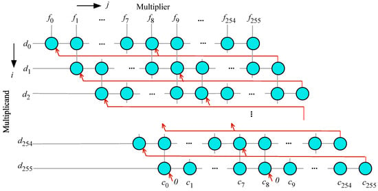
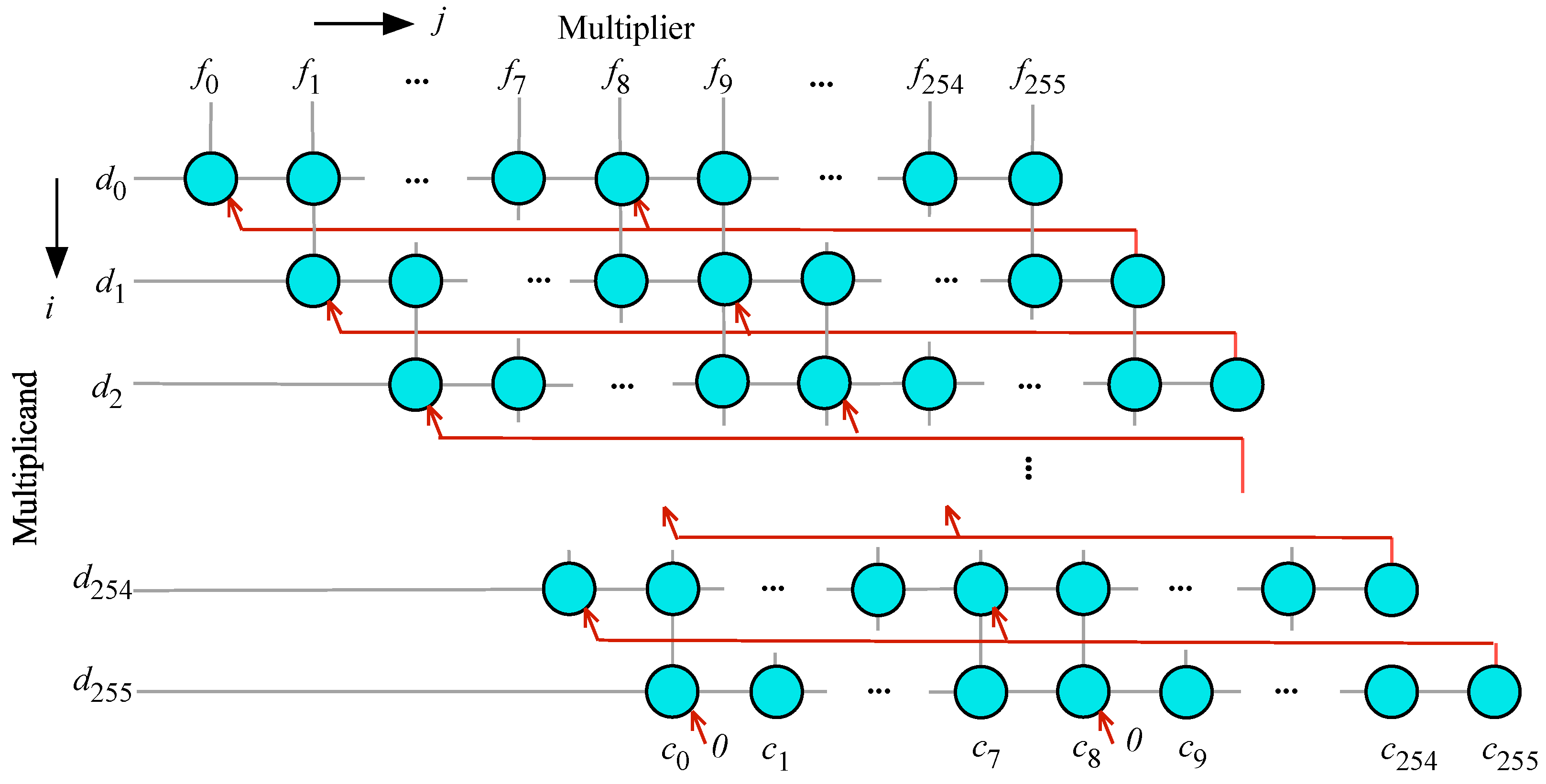
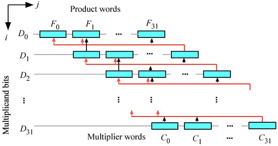
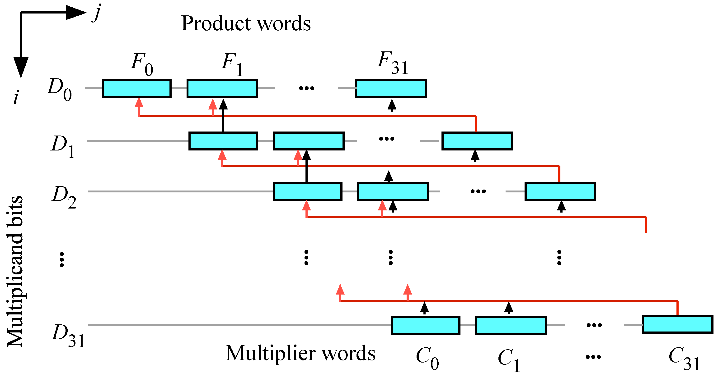
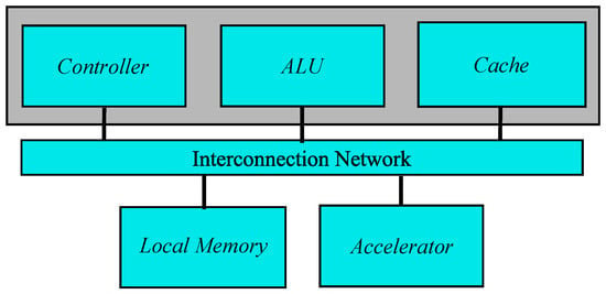
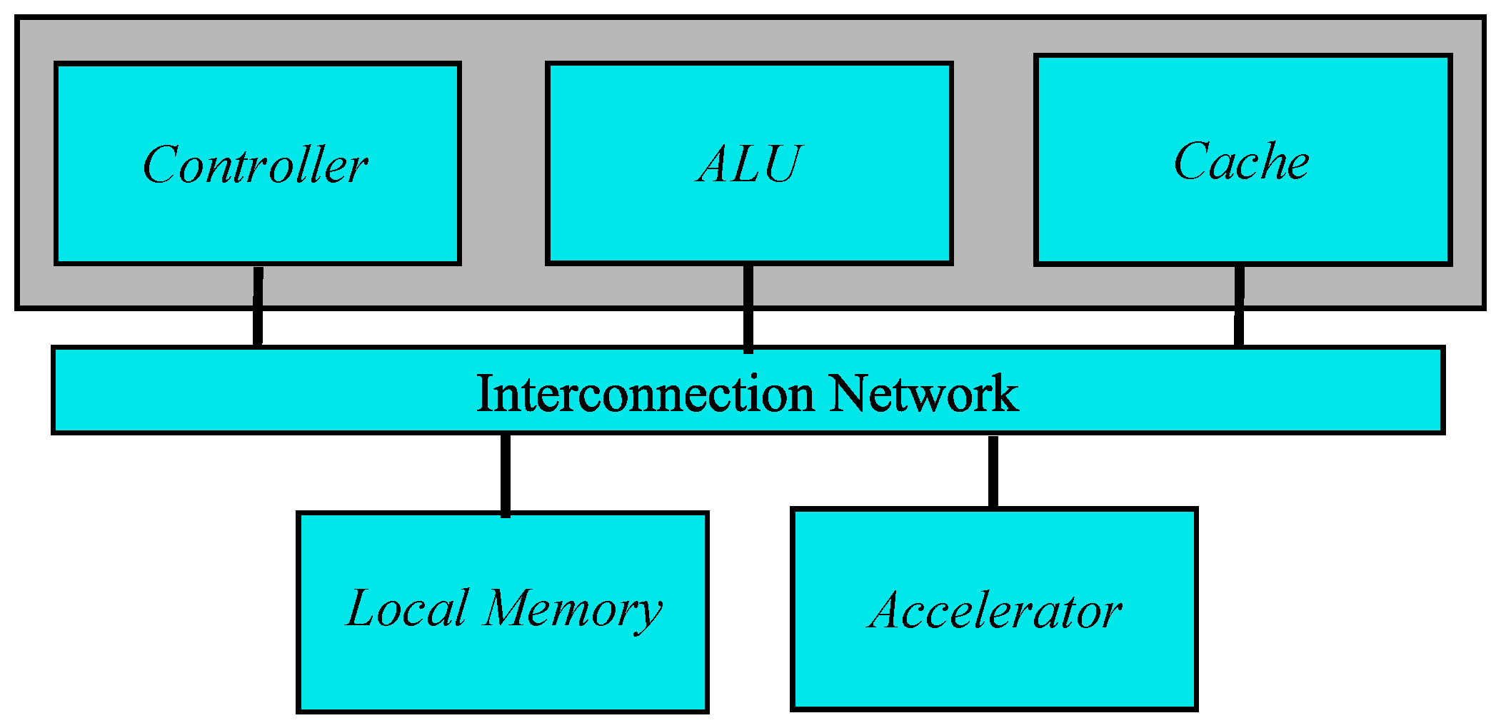
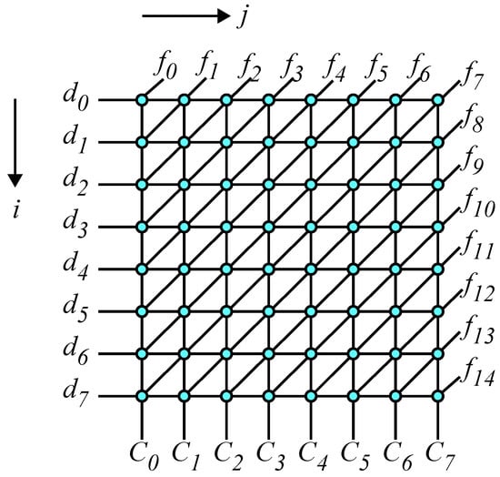
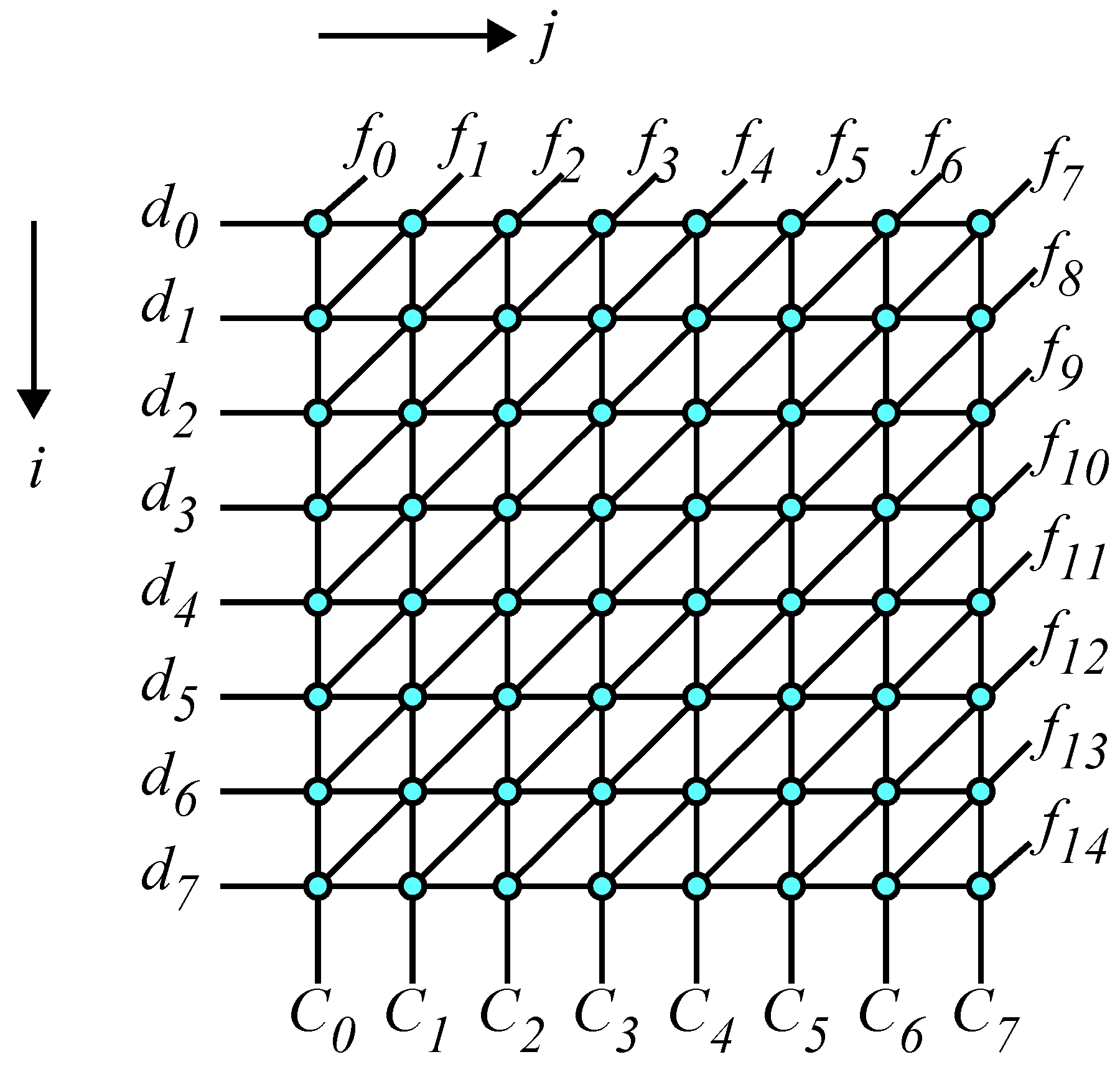
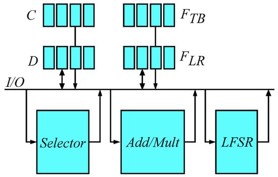
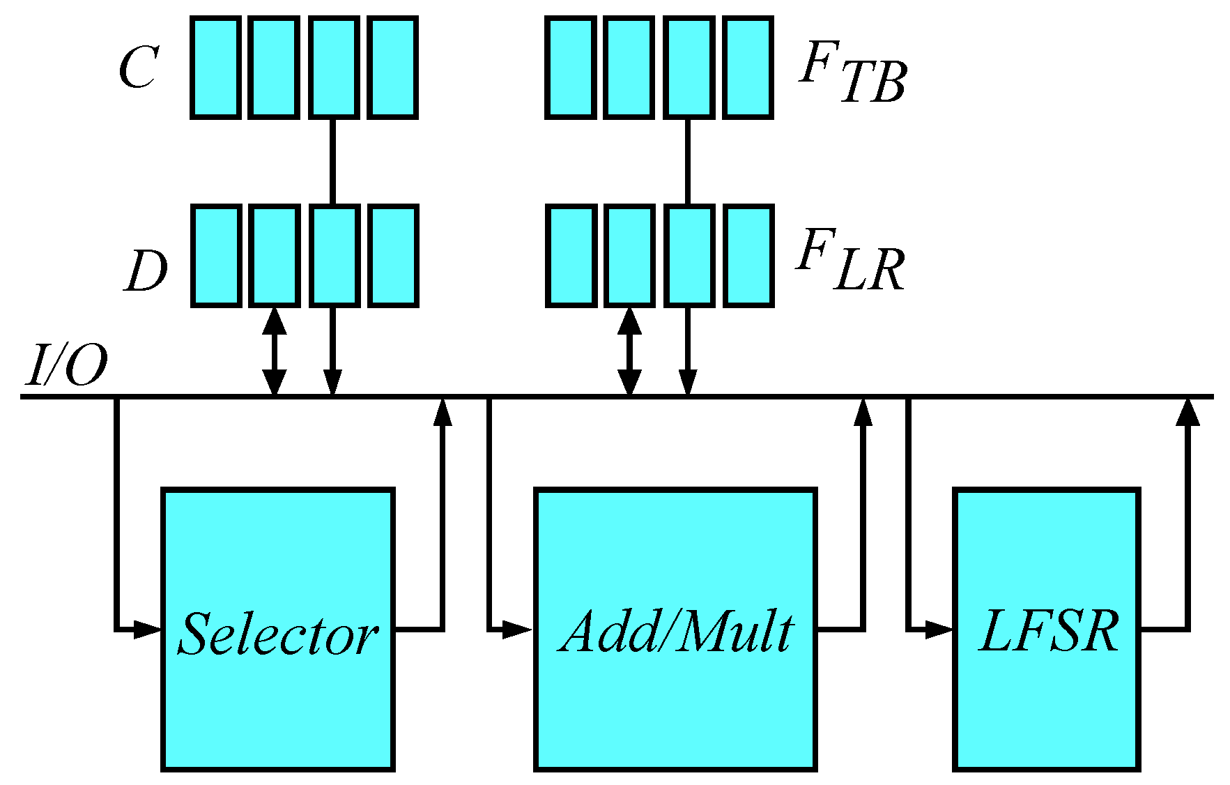
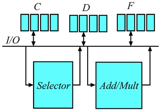
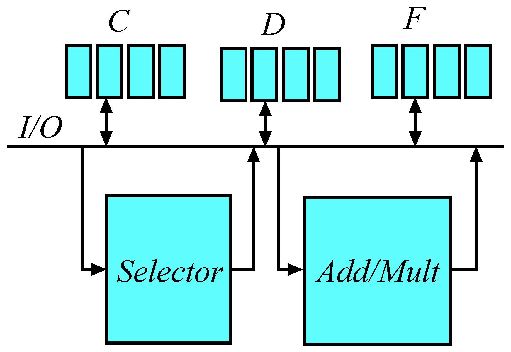
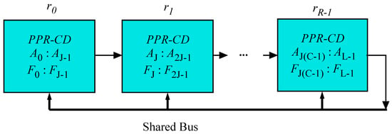
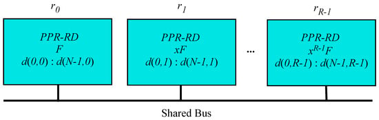


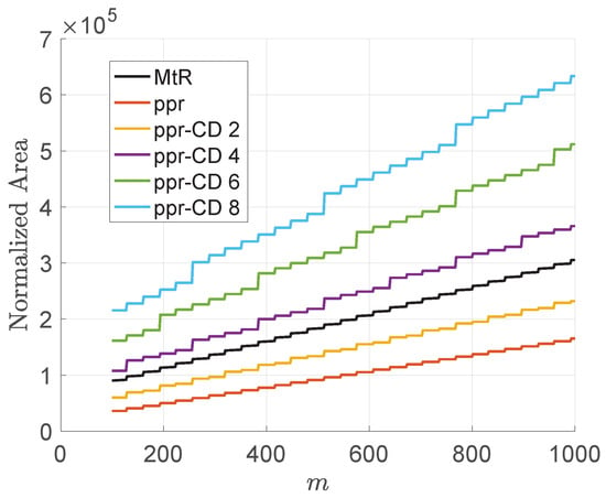
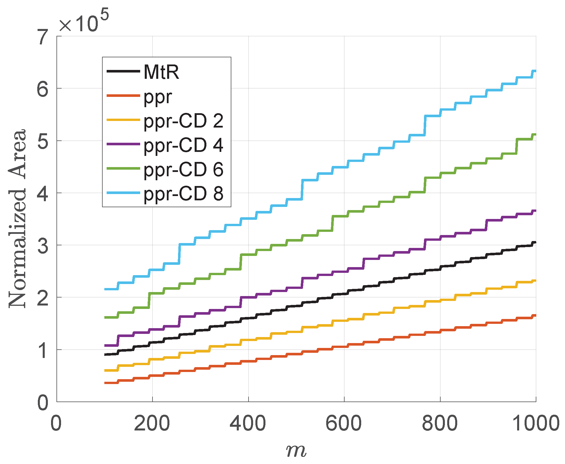
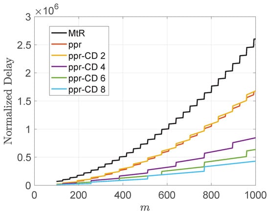
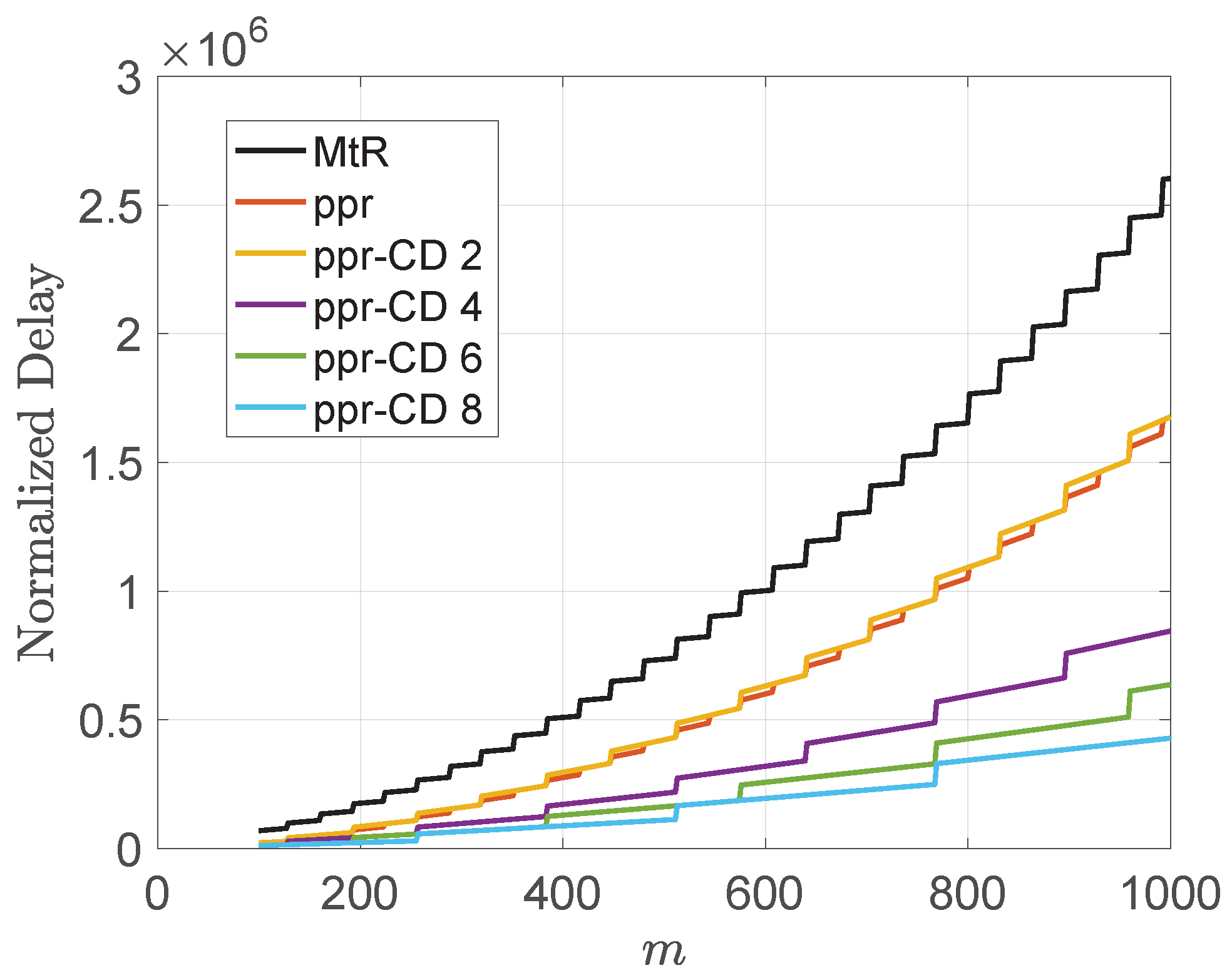
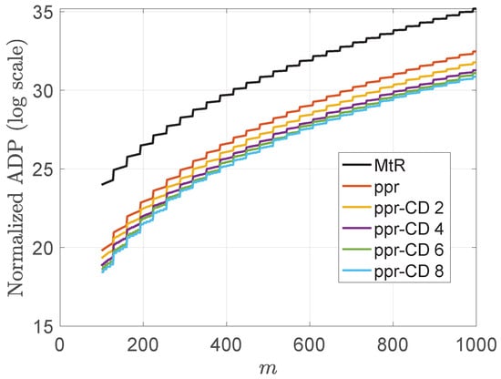
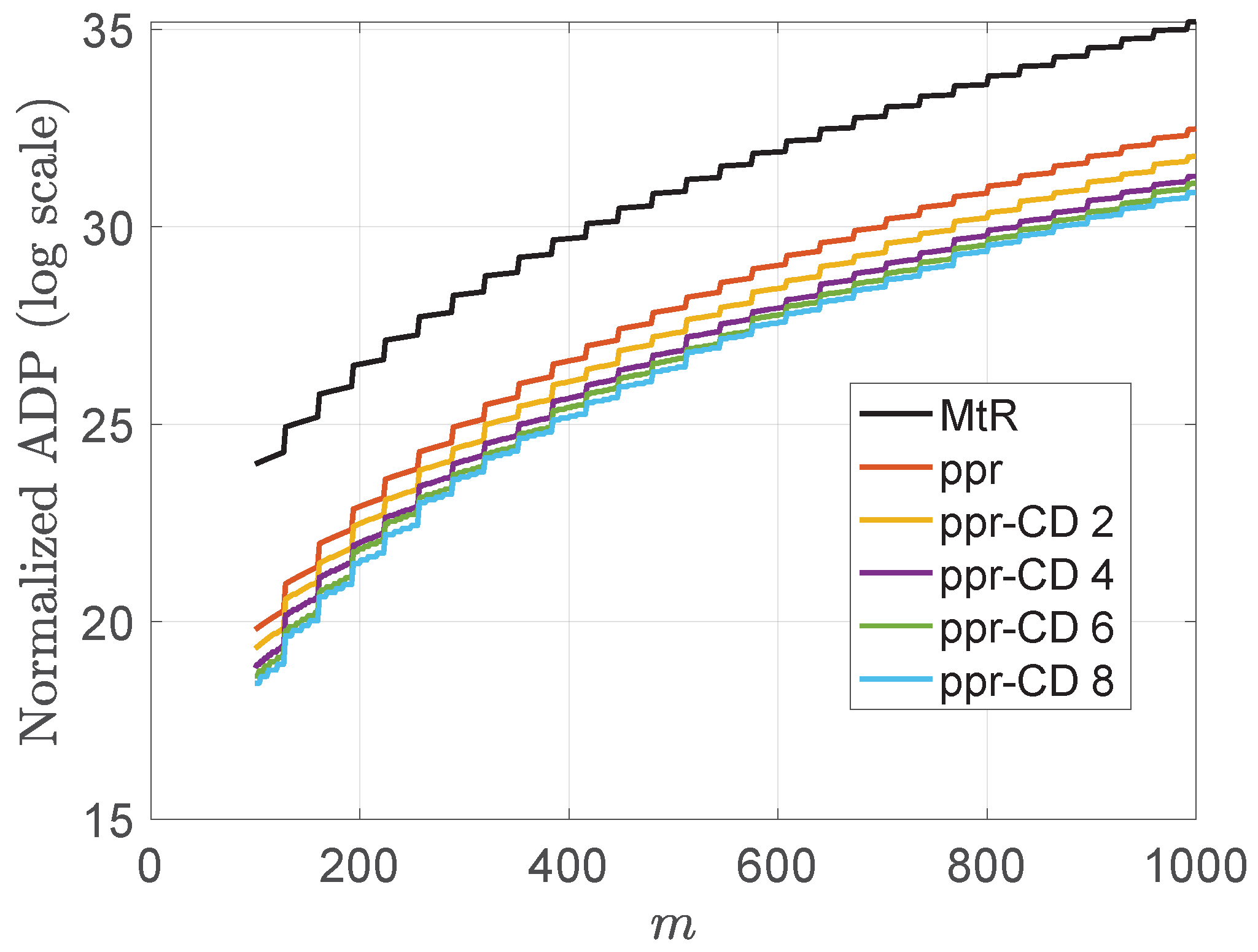
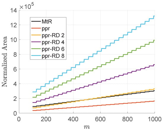
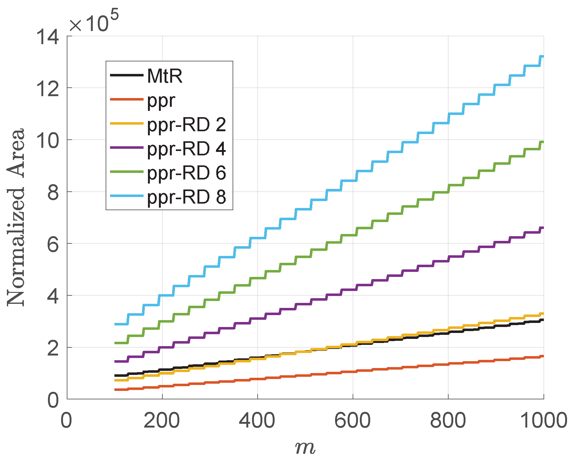
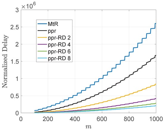
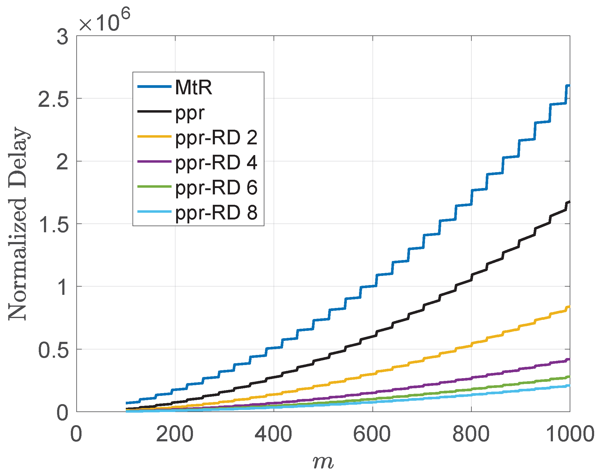
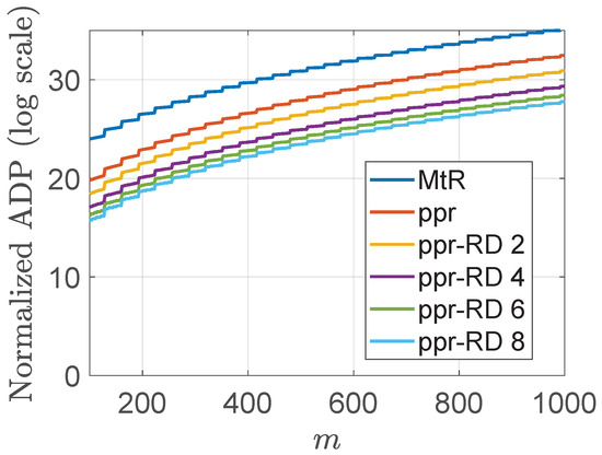
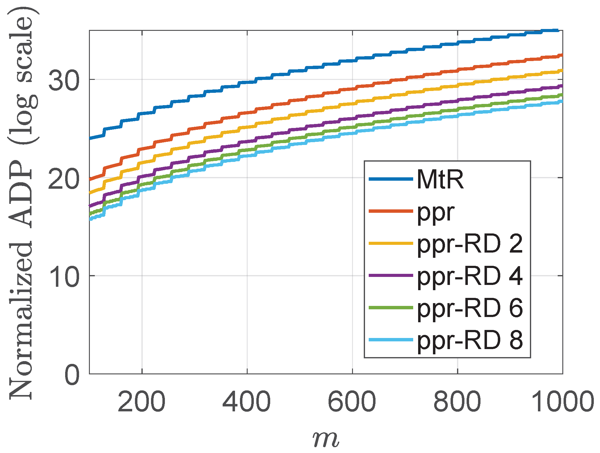
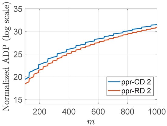
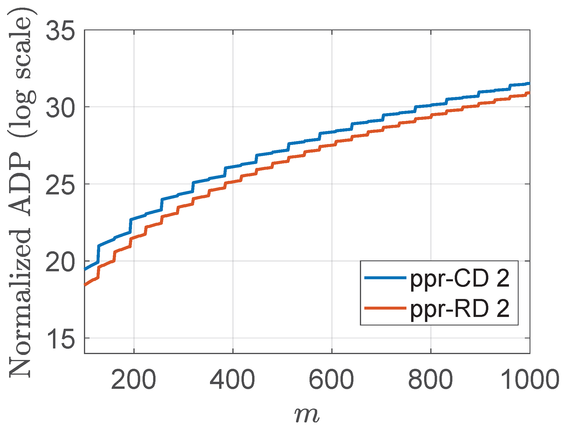
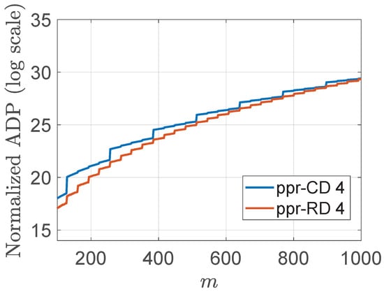
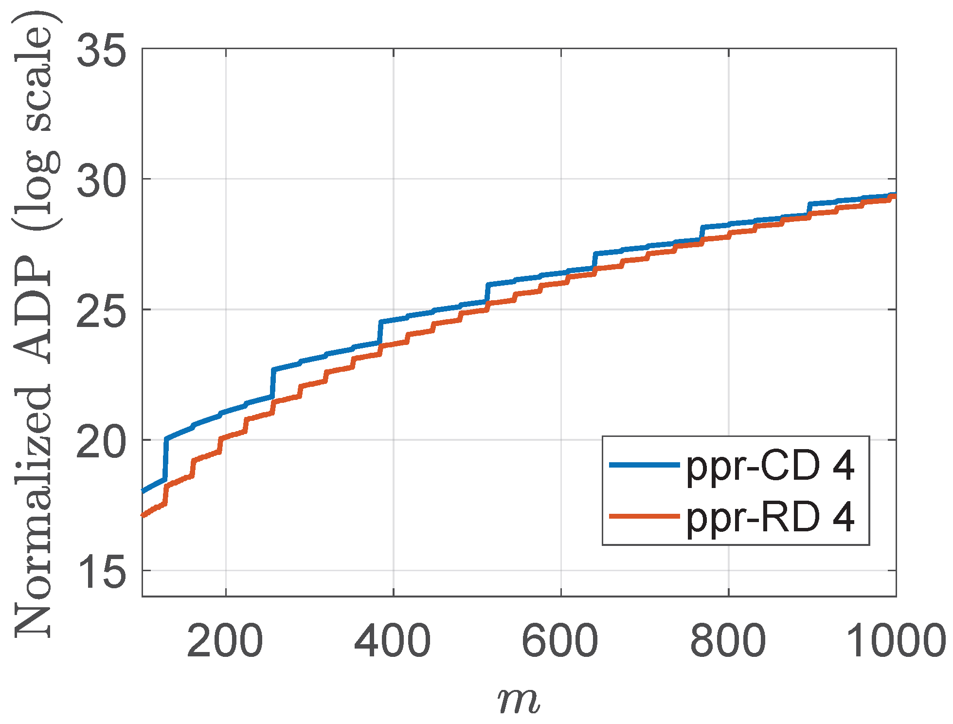
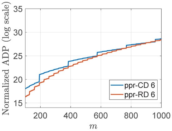
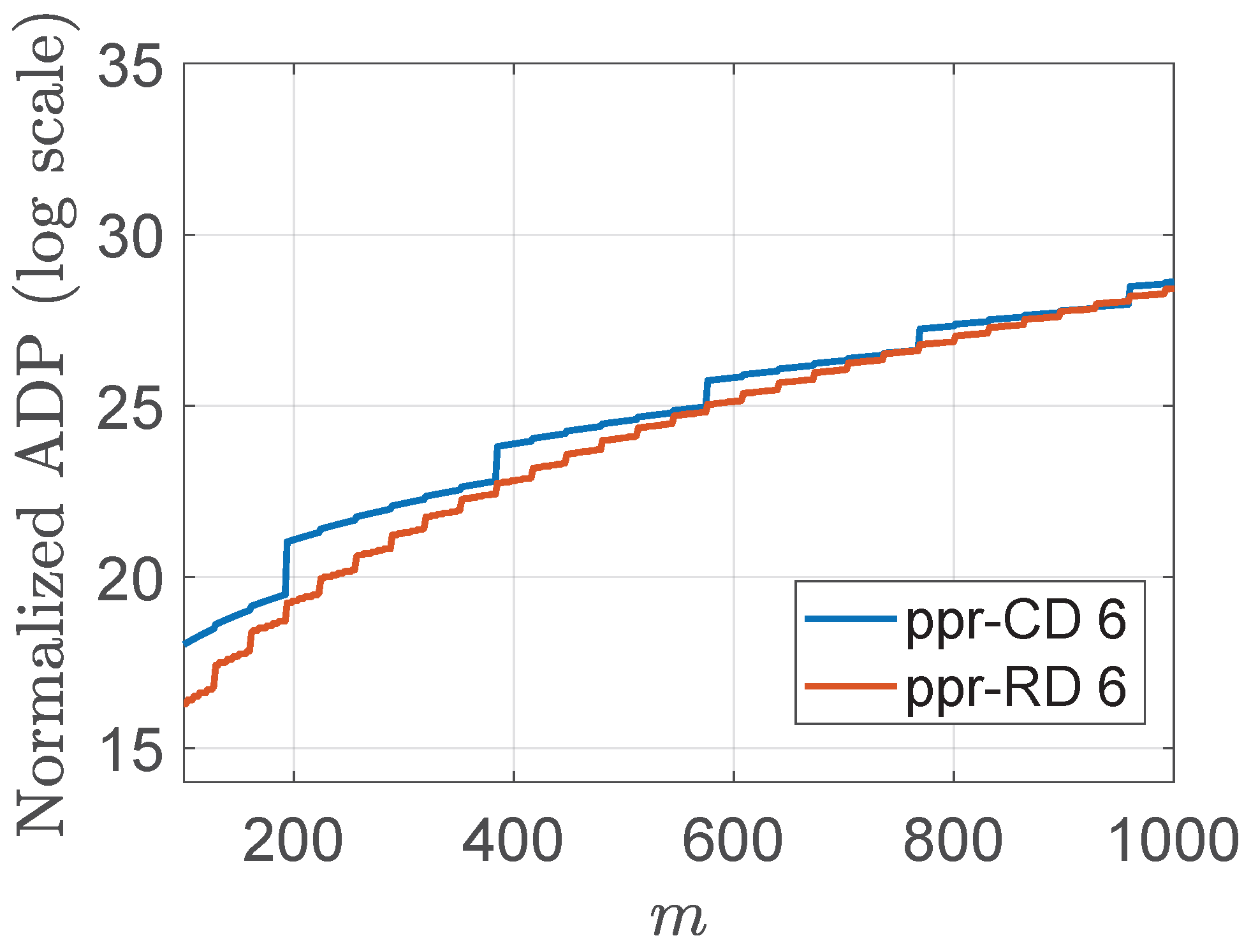
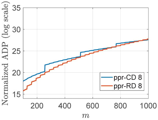
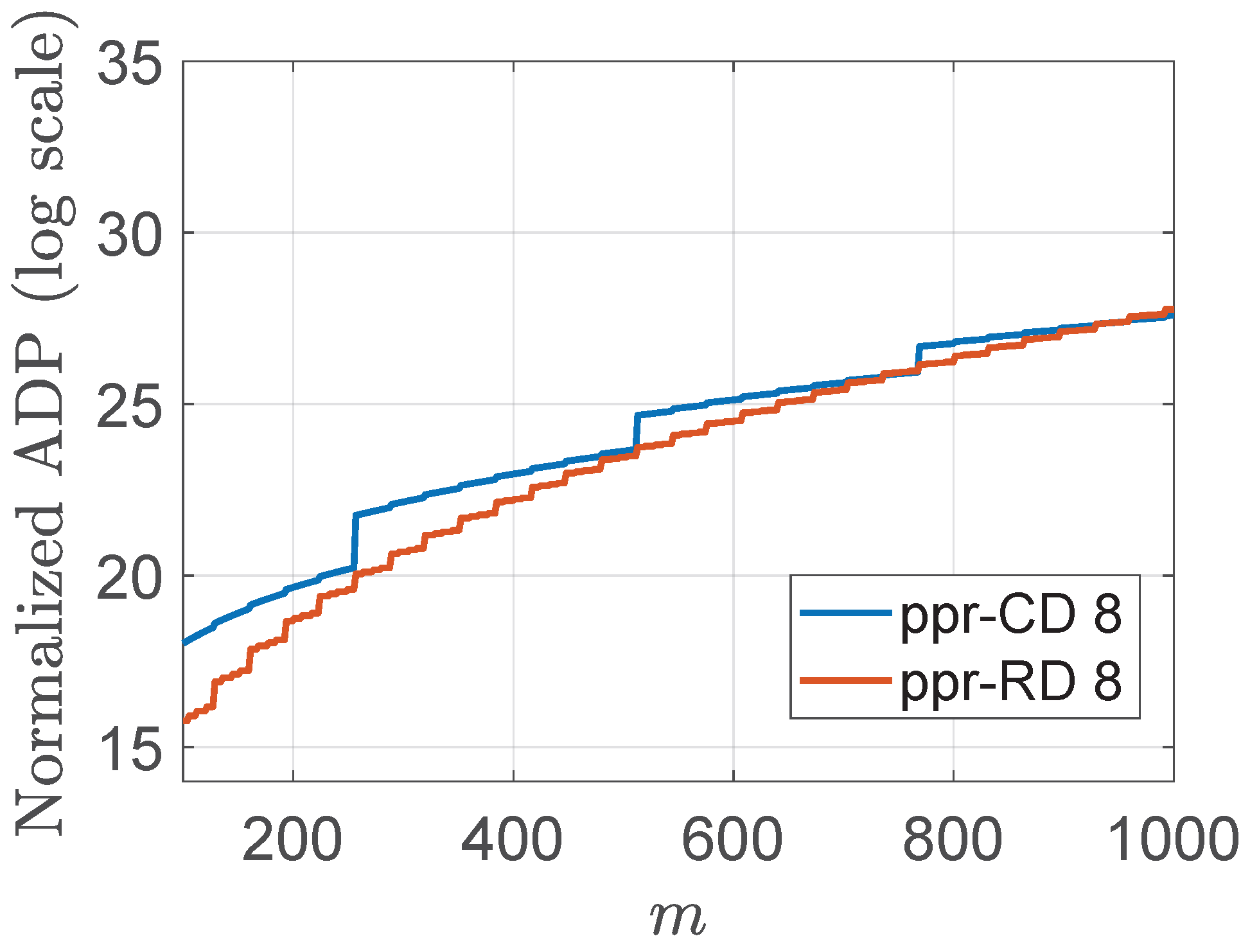

Disclaimer/Publisher’s Note: The statements, opinions and data contained in all publications are solely those of the individual author(s) and contributor(s) and not of MDPI and/or the editor(s). MDPI and/or the editor(s) disclaim responsibility for any injury to people or property resulting from any ideas, methods, instructions or products referred to in the content. |
© 2026 by the authors. Licensee MDPI, Basel, Switzerland. This article is an open access article distributed under the terms and conditions of the Creative Commons Attribution (CC BY) license.