


Abstract
Existing wind power optimization control strategies often lack a qualitative analysis of the relationship between wind power energy and system frequency, which may lead to insufficient or excessive frequency support, thereby reducing the effectiveness of wind power frequency support or triggering a secondary frequency drop. To address this issue, a receiving-end system frequency optimization control strategy based on the available rotor kinetic energy of sending-end wind farms is proposed. First, the mathematical expression of the approximately first-order response in the initial stage of optimized frequency dynamics is clarified. The quantitative relationship between the available rotor kinetic energy of wind farms and the frequency support level is derived, and a target frequency design method is developed by combining a conservative evaluation of effective frequency regulation energy. Second, according to the deviation between the target frequency and the measured frequency, the total frequency regulation demand calculation, the approximate calculation of synchronous generator mechanical power variation, and the wind farms’ frequency regulation command calculation are dynamically executed within each control step. In this way, the outputs of wind farms and synchronous generators are coordinated to regulate the frequency close to the target value. Finally, a simulation model is built in MATLAB/Simulink to verify the effectiveness of the proposed frequency control target design method and control strategy under different operating conditions, as well as their robustness against parameter acquisition errors, communication delays, and power disturbance estimation errors.
1. Introduction
With the accelerated advancement of the global energy transition, renewable energy represented by offshore wind farms (OWFs) has developed rapidly. Due to the limited development potential of nearshore OWFs, OWF development has shown a trend toward deep-sea and far-offshore areas in recent years. As the offshore distance increases, modular multilevel converter-based high-voltage direct current (MMC-HVDC) has become the main approach for OWF power transmission. However, the increasing penetration of OWFs and the isolation effect of DC systems significantly reduce the equivalent inertia of the system. After active power disturbances such as sudden load increases or generator tripping, frequency fluctuations become more severe, which may easily lead to frequency limit violations [1,2,3,4,5,6,7,8]. Therefore, it is urgent to exploit the frequency regulation potential of sending-end OWFs to provide support for the receiving-end system.
Existing strategies that enable OWFs to provide short-term frequency support using rotor kinetic energy can be classified into two categories, i.e., emulating the synchronous generator (SG) and coordinating with SG. Strategies that emulate the SG mainly include droop control, virtual inertia control, fast frequency response and virtual synchronous generator control. Droop control is used to emulate the active power–frequency droop characteristic of the SG governor, and relatively long-duration frequency support is provided after system frequency deviations are detected. A multi-segment droop control strategy has been proposed to replace synthetic inertia, thereby improving the reliability of frequency regulation control [9,10]. Virtual inertia control regulates the active power of OWFs by detecting the rate of change of frequency, such that the inertial response process in which the SG rotor releases or absorbs kinetic energy is emulated [11]. Fuzzy control has also been introduced into virtual inertia control in some studies to improve the frequency response performance of wind turbines [12]. However, virtual inertia control mainly improves the rate of change of frequency, while its effect on raising the frequency nadir is limited. Fast frequency response control is used to emulate the rapid power response characteristic of the SG after an active power disturbance. After a disturbance is detected, a step power response is rapidly provided and maintained for a certain period, after which an appropriate power recovery process should be designed. In early studies, the frequency regulation strategy for OWFs was designed such that, after a step response was maintained for a certain period, the power was reduced in a stepwise manner and the control mode was switched back to maximum power point tracking (MPPT) [13]. However, this may lead to a secondary frequency drop. To address this issue, the analytical relationship between the exit time of fast frequency response and the secondary frequency drop has been derived in some studies, and the optimal exit time that is beneficial for minimizing the secondary frequency drop has been determined [14]. Furthermore, a relatively complete implementation strategy has been proposed by considering step-response power setting, model parameter estimation, and other factors [15]. Virtual synchronous generator control enables wind power to exhibit inertia response and primary frequency regulation capability similar to those of synchronous generators by emulating the rotor motion equation, inertia link, and damping characteristics of synchronous generators. Some scholars have comprehensively summarized the modeling, control, and stability issues of virtual synchronous generator control [16]. Overall, since the above SG-emulating strategies are all designed based on the operating characteristics of SGs, the flexible regulation capability of OWFs is constrained to some extent.
Control strategies coordinated with SGs are intended to exploit the regulation flexibility of wind turbines. Existing studies have proposed optimized control strategies for OWFs that are beneficial for improving frequency regulation performance. In early studies, frequency shaping control was proposed for energy storage systems, by which the frequency nadir can be eliminated, and the rate of change of frequency can also be controlled to the desired value [17]. However, sufficient energy capacity is required for the energy storage system, and thus this method is not fully applicable to frequency regulation strategies for OWFs. Some researchers have proposed planning the frequency trajectory in advance under large disturbances, along with corresponding inverter control strategies [18]. However, the quantitative relationship between renewable energy and the frequency trajectory is not considered, which may lead to insufficient energy. Some studies have established an optimization model with the objective of maximizing the frequency nadir of the power system. Based on particle swarm optimization, it was found that the optimal frequency dynamics exhibit an approximately first-order response in the initial stage [19]. An implementation strategy was then designed using mathematical fitting methods, and subsequent studies further investigated control parameter tuning and multi-machine coordinated implementation [20]. However, the real-time solution of the optimization model imposes a heavy computational burden, and the underlying physical mechanism has not been sufficiently analyzed. The general form of the optimal frequency trajectory under the objective of maximizing the frequency nadir has been demonstrated by proof by contradiction [21], and the conclusion is consistent with the aforementioned studies. On this basis, an OWF control method was derived in reverse based on the system frequency response, and an optimal frequency trajectory tracking control strategy was further proposed [22]. However, the impact of wind energy capture loss was not considered, and the quantitative relationship between the wind power energy and the equation of the frequency reference curve was not provided. Recent studies have revealed, through energy process analysis, that the optimal timing for improving the frequency nadir using the limited energy of wind turbines should lie between the inertial response and primary frequency regulation of SGs. Accordingly, a lagged inertia control strategy for wind turbines has been proposed to compensate for the energy deficiency caused by the delayed response of primary frequency regulation [23].
In the above literature, it can be observed that the flexibility of SG-emulating control strategies is limited. Although a series of studies have been conducted on control strategies coordinated with SGs, and it has been verified that the optimal frequency dynamics are characterized by regulating the frequency into an approximately first-order response in the initial stage, the quantitative relationship between the frequency regulation energy of OWFs and the frequency dynamics has not been analyzed. Consequently, the frequency regulation performance is significantly affected by system parameter estimation, control parameter tuning, and other factors. To address the above issues, this paper proposes an optimal frequency control strategy for OWFs integrated via MMC-HVDC based on available rotor kinetic energy. The main contributions are as follows:
(1) A frequency control target design method based on the available rotor kinetic energy of OWFs is proposed. To improve the frequency nadir, a target frequency expression that is approximately a first-order response in the initial control stage is constructed. On this basis, the quantitative relationship between the available rotor kinetic energy of OWFs and the target frequency level is derived, providing a reference for the subsequent control strategy.
(2) An evaluation method for the proportion of effective frequency regulation energy to the released rotor kinetic energy is proposed, considering the complexity and variability of OWFs frequency regulation strategies. First, the rotor speed variation curve under complex strategies is approximately modeled. On this basis, the calculation method of effective frequency regulation energy is characterized using a quartic fitting method. Finally, conservative estimates of the proportion under different wind speeds are obtained through simulations considering flexible control of OWFs, providing a basis for parameter setting in target frequency design.
(3) A frequency tracking control strategy for OWFs coordinated with SGs is proposed. First, according to the deviation between the target frequency and the measured frequency within each control step, the total frequency regulation power required from OWFs and SGs is calculated. Then, the mechanical power variation of SGs is approximately calculated. Finally, the frequency regulation power command for OWFs is calculated in a receding manner at each control step, so that the actual frequency is regulated around the target frequency.
2. Frequency Dynamics and Sources of Frequency Regulation Energy
2.1. Frequency Dynamic Model of the Receiving-End System
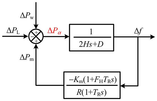
The system frequency response model including OWFs, SGs, and loads is shown in Figure 1 [24].
Figure 1.
System frequency response model with OWFs.
Accordingly, when the spatial distribution differences in frequency are neglected, the system frequency dynamics considering OWF support can be expressed as
where Δf is the deviation between the measured system frequency and the rated frequency, ΔPm denotes the mechanical power increment of SGs, ΔPw is the frequency regulation power of the sending-end OWFs, ΔPL denotes the load power variation, ΔPa represents the sum of the power contributions from the load, SGs, and sending-end OWFs, and H and D denote the system inertia time constant and damping coefficient, respectively.
The mechanical power increment of SGs is calculated using the classical single-machine equivalent model, i.e.,
where Km is the mechanical power gain of SGs, FH denotes the power contribution proportion of the high-pressure turbine section, TR is the reheat time constant, and R is the droop coefficient. For a multi-machine system, the equivalent parameters in the model can be obtained by capacity-weighted calculation.
2.2. Frequency Regulation Energy of Offshore Wind Farms Integrated via MMC-HVDC
The frequency regulation energy of OWFs integrated via MMC-HVDC mainly includes the rotor kinetic energy of the sending-end wind turbines and the energy stored in the capacitors of the MMC-HVDC system. Since the latter is much smaller than the former, this study mainly exploits the energy of the sending-end OWFs to provide frequency support in coordination with receiving-end SGs. In addition, since a sudden load decrease can be balanced by reducing the output power of SGs and other measures, whereas a sudden load increase or generator power reduction is more difficult to handle, this paper mainly takes a sudden load increase as an example for analysis.
When OWFs participate in frequency regulation, the energy sources include reserved energy and the rotor kinetic energy stored in the turbines themselves. Reserving energy reduces the economic benefit of power generation, and operating conditions in which the wind speed reaches or exceeds the rated value of wind turbines account for only a small portion of the annual operating time of OWFs. Therefore, this paper mainly focuses on wind turbines operating in the MPPT mode and investigates a control strategy that utilizes their rotor kinetic energy to support system frequency.
Under normal operating conditions, the rotor speed of wind turbines operating in the MPPT mode is only related to the wind speed, and the system operates stably. After an active power disturbance occurs, wind turbines provide support to the system by decelerating and releasing their rotor kinetic energy. The maximum releasable rotor kinetic energy can be expressed a,
where Ew,max denotes the maximum releasable rotor kinetic energy, Ht and Hg denote the inertia time constants of the wind turbine and the wind generator, respectively, ωr is the rotor speed of the wind turbine expressed in per-unit form, ωmin denotes the minimum allowable rotor speed of the wind turbine expressed in per-unit form, which is generally 0.7 p.u.
3. Frequency Control Target Design Based on the Available Rotor Kinetic Energy of Sending-End OWFs
3.1. General Form of the Frequency Control Target
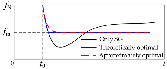
Since the rotor kinetic energy stored in OWFs can provide only short-term and limited support, it is necessary to explore efficient methods for utilizing this energy. At present, existing studies have investigated the optimal frequency dynamics in the inertia and primary frequency regulation stages with wind power participation, aiming to maximize the frequency nadir of the power system through optimization-based solutions or theoretical derivations [19,20,21,22,23]. The schematic diagram is shown below.
As shown in the above figure, the optimized frequency trajectory derived in existing studies for improving the frequency nadir is characterized by a rapid decline followed by an approximately maintained level. In this study, this trajectory is taken as the control target to analyze the setting method of the frequency level, and a novel coordinated control method is proposed.
In Figure 2, fN denotes the rated system frequency, fm denotes the frequency value in the maintained-level stage, and t0 is the time instant when the active power disturbance occurs. The theoretically optimal frequency dynamics are shown by the blue solid line. However, the abrupt frequency change at the turning point may cause maloperation of protection devices. Therefore, in this paper, the optimal frequency dynamics are approximately represented by the first-order inertial response shown by the red dashed line, which is expressed as follows
where f*(t) denotes the dynamic function of the optimized frequency trajectory, which is also used as the control target in the subsequent control strategy of this paper. Δfm = fm − fN represents the deviation of the frequency level from the nominal frequency, and τ is the time constant of the approximately first-order target-frequency function, which is affected by the frequency decline rate. Based on simulation experience with common system parameters, τ = 0.5 s can well reflect most frequency decline cases. It can be observed from the above equation that the control target design can be completed by properly determining Δfm.
Figure 2.
Schematic diagram of the optimized frequency trajectory for improving the frequency nadir.
It should be noted that the above frequency dynamic expression does not specify the ending time of the maintained frequency level. Instead, it is naturally determined by the intersection time between the OWF’s support power and the MPPT curve. In the subsequent control design, when the support power is detected to be equal to the MPPT power, the controller can be switched to the MPPT mode, thereby achieving a smooth transition of the frequency trajectory.
3.2. Frequency Control Target Level Setting Based on the Available Rotor Kinetic Energy of Sending-End OWFs
The amount of available rotor kinetic energy of the sending-end OWFs obviously affects the feasible value of Δfm in Equation (4). Specifically, a larger available rotor kinetic energy can support a larger Δfm, and vice versa. Therefore, it is necessary to investigate the mathematical relationship between the available rotor kinetic energy of the OWFs and the frequency support level, so that frequency support can be provided while ensuring the rotor speed safety of wind turbines. The derivation is given as follows.
First, by integrating Equation (1) over the effective OWFs support interval [t0, ts], the following expression is obtained:
where t0 is the starting time at which effective support is provided by the OWFs, and ts denotes the ending time of effective OWFs support, i.e., the time instant when ΔPw = 0. In conventional OWFs frequency regulation control strategies, the deadband is relatively small; thus, it can be approximately assumed that t0 = 0. Meanwhile, before the disturbance event occurs, the system frequency is generally stabilized at the rated frequency, i.e., Δf(t0) = Δf(0) = 0. Therefore, the above expression can be simplified as
By integrating Equation (2), the following expression is obtained:
By substituting Equation (7) into Equation (5), the following expression is obtained:
After the frequency is regulated to follow the optimal frequency dynamics shown in Figure 2, Δf(ts) = Δfm is satisfied. Considering that ts τ, the frequency decline time before entering the maintained-level stage is relatively short compared with the duration of frequency regulation. Therefore, the following approximation can be made.
Similarly, the frequency changes very slowly around the ending time ts of effective OWFs support, satisfying s → 0. By performing a Taylor expansion of 1/(1 + TRs) in Equation (2) around s = 0 and retaining the first-order approximation, the transfer function in Equation (2) can be transformed into
By neglecting the second-order terms and transforming it into the time-domain expression, the following equation is obtained:
Around ts, dΔf(ts)/dt ≈ 0 is satisfied. Therefore, we have
By substituting Equations (9) and (12) into Equation (8) and rearranging, the following expression is obtained:
Equation (13) reflects the quantitative relationship between the effective support energy of the OWFs and the frequency deviation level, where the ending time of effective OWF support, ts, varies with the control strategy. To simplify the analysis, ts is set to 20.0 s in this paper by referring to existing studies and the typical time scale of OWFs participation in frequency regulation; subsequent derivations and simulations will, respectively, demonstrate the influence of ts on Δfm and the rationality of the value chosen here. Obviously, a larger effective support energy provided by the OWFs corresponds to a higher supportable frequency level. However, on the one hand, the effective support energy of the OWFs is constrained by their stored rotor kinetic energy; on the other hand, considering that the OWFs only provide short-term support, the supported frequency level should not be higher than the quasi-steady-state frequency. Therefore, the final calculation method for the frequency deviation level is given as follows:
where h denotes the conservative proportion of the effective OWFs frequency regulation energy to the maximum releasable rotor kinetic energy. Its value varies with the frequency regulation strategy and wind speed. In this paper, h is set to 0.7, and its evaluation method will be described in detail in the next subsection.
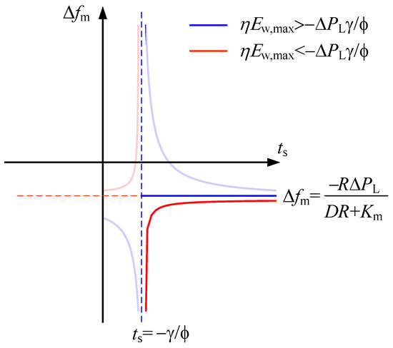
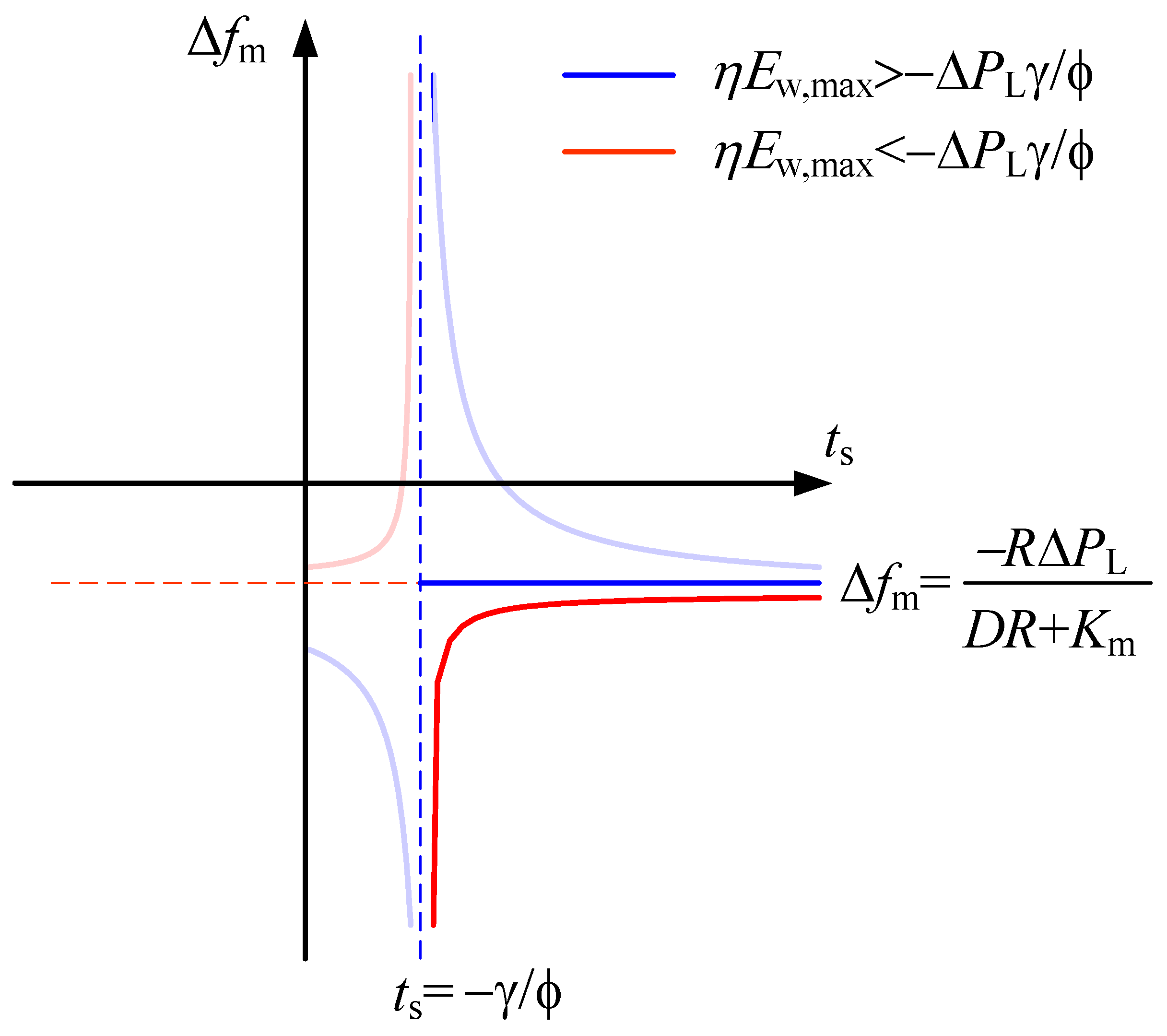
Obviously, the tuning value of Δfm in Equation (14) is affected by the value of ts. However, in practical control, the effective frequency regulation time is complex and variable, making it difficult to dynamically adjust ts and tune Δfm for a specific strategy. Therefore, ts should be selected to ensure the reliability of the target frequency calculation method under common control strategies. To facilitate graphical representation, let the denominator of the left-hand expression inside the brackets in Equation (14) be simplified as γ = 2H + KmTR(FH − 1)/R and ϕ = D + Km/R. Based on calculations using common system parameters, it can be seen that γ < 0 and ϕ > 0. On this basis, the function curve of Δfm with respect to ts corresponding to Equation (14) is plotted in the figure below.
As shown in Figure 3, the function determined solely by Equation (13) exhibits a hyperbolic shape. Specifically, the blue curve corresponds to the case with larger effective frequency regulation energy of the OWFs, while the red curve corresponds to the case with smaller effective energy. The vertical asymptote is ts = −g/f, whose typical value is approximately 2–3 s. Therefore, the time range of interest in the design of the frequency control target lies to the right of the vertical asymptote. Further considering a smaller quasi-steady-state frequency, the final curves correspond to the dark blue and red lines in the figure above. In other words, when the effective frequency regulation energy of the OWFs is sufficiently large, the frequency can be supported close to the quasi-steady-state frequency and is independent of ts. When the effective frequency regulation energy of the OWFs is relatively small, the supported frequency level is negatively correlated with ts. However, it is difficult to analytically determine which value of ts can cover common control scenarios. Therefore, simulations are required to determine a relatively reasonable value of ts, so that the target frequency can always be achieved when it is lower than the tuned value, while it is difficult to achieve in most cases when it is higher than the tuned value. This ensures the implementation of target-frequency control while avoiding unnecessary consumption of OWFs frequency regulation energy. The quantitative verification of ts will be provided in the simulation section. Here, the conclusion is given first to facilitate the subsequent derivation, namely ts = 20.0 s.
Figure 3.
Function plot of Δfm with respect to ts corresponding to Equation (14).
It should be noted that the disturbance magnitude is required as an input when the frequency level setting value is calculated using the above equation. Relatively mature estimation methods for this parameter have been reported in the existing literature, and this issue is not the focus of this paper. Further improving the existing target-frequency design method and control strategy by incorporating disturbance sensing methods will be one of the authors’ future research directions.
3.3. Conservative Evaluation of the Proportion of Effective Frequency Regulation Energy to Released Rotor Kinetic Energy Under Complex and Variable OWFs’ Control Strategies
When OWFs provide support using rotor kinetic energy, the maximum releasable rotor kinetic energy can be calculated based on Equation (3). However, since the decrease in rotor speed also leads to wind energy capture loss, the energy actually used for system frequency support is the integral of the positive part of the support power, which is defined as the effective frequency regulation energy. The proportion of the effective frequency regulation energy to the released rotor kinetic energy varies with wind speed and frequency regulation strategy. To analyze the conservative value of this proportion, an effective frequency regulation energy evaluation method for OWFs based on differentiated rotor speed curves is proposed in this paper.
3.3.1. Approximate Modeling of Rotor Speed Curves Characterizing Complex and Variable Controls
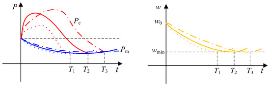
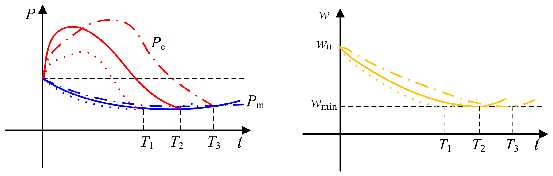
As shown in Figure 4, when the effective frequency regulation energy of wind turbines at a given wind speed is evaluated, different control strategies lead to different electromagnetic power curves and different times for the rotor speed to decrease to the minimum value of 0.7 p.u. Consequently, different variation trends of the captured mechanical power of the wind turbines are produced, exhibiting complex and variable characteristics.
Figure 4.
Wind turbine power and rotor-speed variations under different control strategies.
In the proposed method, no specific OWF frequency regulation control strategy is predefined. Instead, only the rotor speed reduction process of wind turbines is considered, and approximate first-order dynamics with different time constants are used to characterize the differences in rotor speed curves and thus represent different control strategies. The model is given as follows.
where T is the typical time during which wind turbines participate in frequency support, and ω0 denotes the initial rotor speed of the wind turbine, expressed in per-unit form. In this paper, T is set to 10 s, 15 s, 20 s, 25 s, 30 s, 35 s, and 40 s, respectively, to characterize different commonly used control strategies.
3.3.2. Illustrative Example of Effective Frequency Regulation Energy Calculation Under a Specific Control
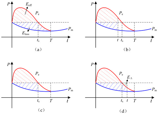
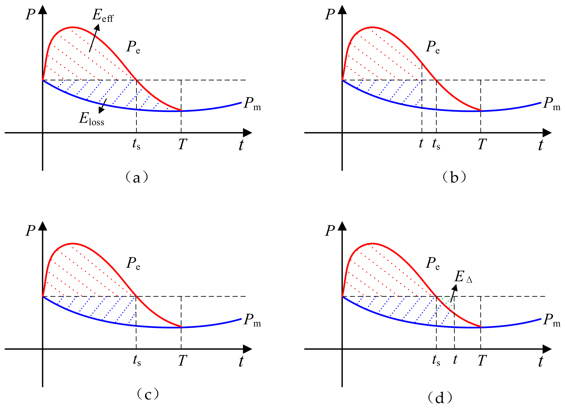
Under a certain control mode at a given wind speed, the calculation process of the effective frequency regulation energy is shown in the above figure. As shown in Figure 5a, the area enclosed by the electromagnetic power and mechanical power curves, i.e., the sum of the red and blue shaded areas, corresponds to the released rotor kinetic energy of the wind turbine at a specific time. The wind energy capture loss corresponds to the area enclosed by the mechanical power and the pre-support power, i.e., the blue shaded area, while the effective frequency regulation energy corresponds to the area enclosed by the electromagnetic power and the pre-support power, i.e., the red shaded area. Therefore, the effective frequency regulation energy at a specific time can be obtained by subtracting the wind energy capture loss from the released rotor kinetic energy.
Figure 5.
Schematic illustration of effective frequency-regulation energy over time. (a) Effective frequency regulation energy during the complete release process; (b) effective frequency regulation energy for t < ts; (c) effective frequency regulation energy at t = ts; (d) effective frequency regulation energy for t > ts.
As shown in Figure 5b, before the first zero-crossing time ts of the electromagnetic power, the effective frequency regulation energy increases with time. As shown in Figure 5c, the effective frequency regulation energy reaches its maximum value at ts. As shown in Figure 5d, after ts, the effective frequency regulation energy obtained by subtracting the wind energy capture loss from the released rotor kinetic energy is smaller than that shown in Figure 5c, because the green shaded area EΔ is additionally subtracted. Therefore, the maximum effective frequency regulation energy of the wind turbine can be obtained by solving for the maximum value on the effective frequency regulation energy curve.
The modeling process corresponding to the above analysis is as follows. When frequency support is provided using the rotor kinetic energy of OWFs, the rotor speed deviates from the MPPT operating point, and the wind energy capture coefficient decreases, resulting in a reduction in mechanical power. Since the variation in the wind energy capture coefficient can be fitted by a quartic polynomial of the tip-speed ratio variation with almost no loss of accuracy [25], the mechanical power loss of OWFs can be approximately expressed as
where ΔPm,w denotes the mechanical power variation of the wind turbine during frequency regulation, i is the exponent, ai is the fitting coefficient of the quartic polynomial, Δl denotes the variation of the tip-speed ratio, Rw is the radius of the wind turbine and vw denotes the wind speed.
During the rotor kinetic energy release stage, the wind energy capture loss can be expressed by the following integral.
where ΔEloss(t) denotes the wind energy capture loss at time t. It should be noted that since the rotor speed variation is modeled as a negative value in Equation (15), the calculated wind energy capture loss is also negative.
Then, the effective frequency regulation energy of OWFs can be expressed as:
where ΔEw,eff(t) denotes the effective frequency regulation energy of the OWFs at time t, ΔEk(t) denotes the released rotor kinetic energy of the OWFs at time t, and JW is the moment of inertia of the wind turbine.
3.3.3. General Characteristics of the Maximum Proportion of Effective Frequency Regulation Energy to Released Rotor Kinetic Energy Under Different Wind Speeds and Control Strategies
Based on the approximate rotor speed representation model in Section 3.3.1 and the effective frequency regulation energy calculation method in Section 3.3.2, simulations are conducted to summarize the general characteristics of the proportion of the maximum effective frequency regulation energy to the released rotor kinetic energy under common wind speeds and control strategies. This provides a basis for selecting the conservative proportion in Equation (14) for control target design.
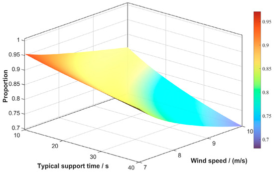
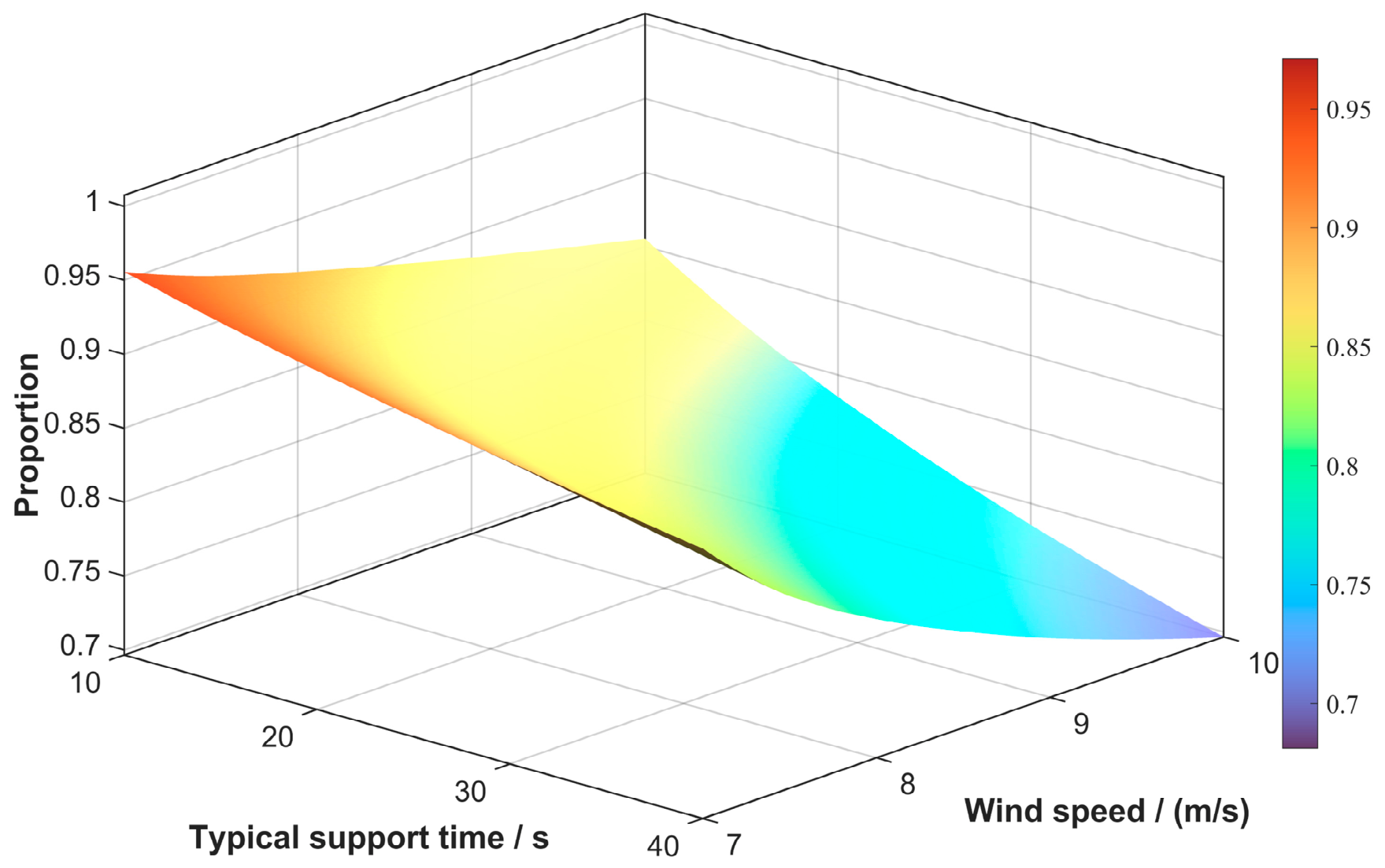
Wind speeds of 7.0, 7.5, 8.0, 8.5, 9.0, 9.5, and 10.0 m/s are selected. Combined with the above support durations T of 10 s, 15 s, 20 s, 25 s, 30 s, 35 s, and 40 s, which are used to characterize different control strategies, the simulation results under different operating conditions are shown as follows.
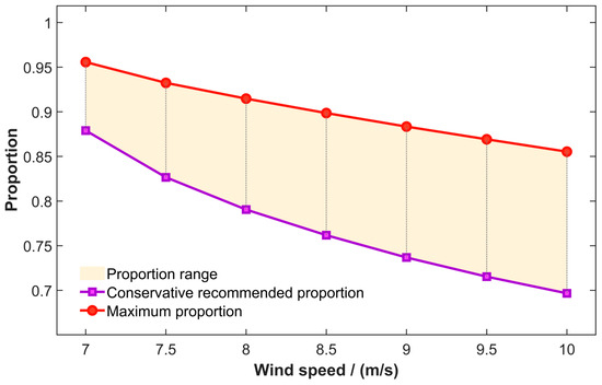
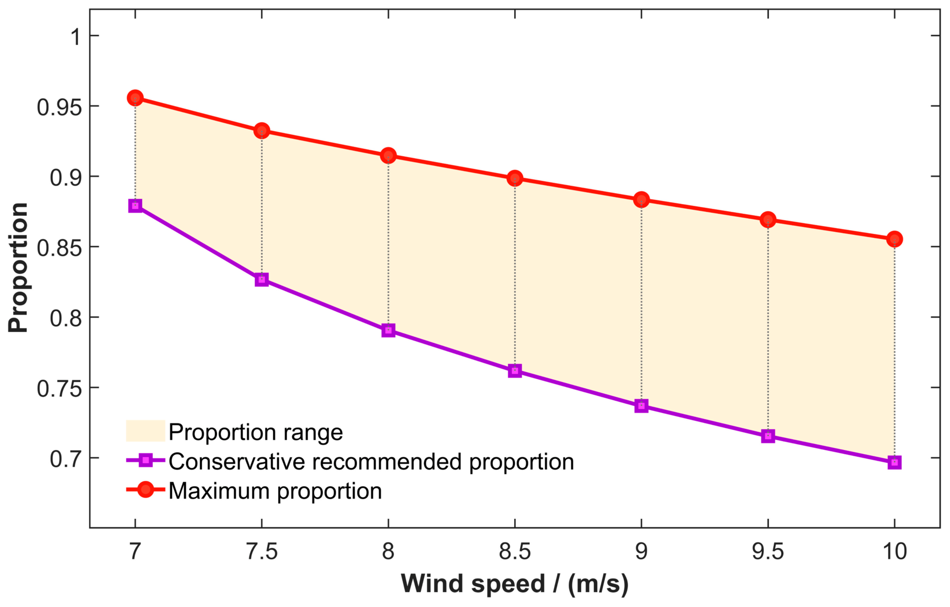
It can be observed from the above figure that, at a given wind speed, the proportion of the maximum effective frequency regulation energy to the released rotor kinetic energy decreases as the support duration increases. For a given support duration, a higher wind speed leads to lower effective frequency regulation energy. In practical power grids, the operating state of wind turbines can be obtained by the controller through wind speed or rotor speed measurements. Therefore, it is necessary to investigate how the conservative proportion should be selected under different wind speeds, as shown in the following figure.
Obviously, at a specific wind speed, the proportion of the maximum effective frequency regulation energy to the released rotor kinetic energy varies with the control strategy. By comprehensively considering the common OWFs support duration range, the conservative value of this proportion under different wind speeds can be determined according to the conservative recommended proportion shown in the above figure. In this study, to conservatively evaluate the maximum effective frequency regulation energy proportion under different wind speeds and control strategies, the proportional coefficient is finally selected as 0.7 based on the above figure, which serves as the basis for setting h in Equation (14).
It should be noted that Figure 6 and Figure 7 are included to provide the simulation basis for the selection of h in Equation (14). Figure 6 shows the variation of the maximum effective frequency regulation energy proportion under different wind speeds and support durations, and Figure 7 further gives the conservative recommended proportion. These results are used to demonstrate that only part of the released rotor kinetic energy can be effectively utilized for frequency regulation, thereby justifying the adoption of a conservative h in the target-frequency design.
Figure 6.
Effect of wind speed and support duration on the maximum effective frequency regulation energy ratio.
Figure 7.
Conservative selection of maximum effective frequency regulation energy ratio.
4. Frequency-Tracking Control of Sending-End OWFs Coordinated with Receiving-End SGs
4.1. Overview of the Control Strategy
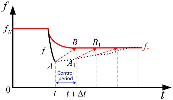
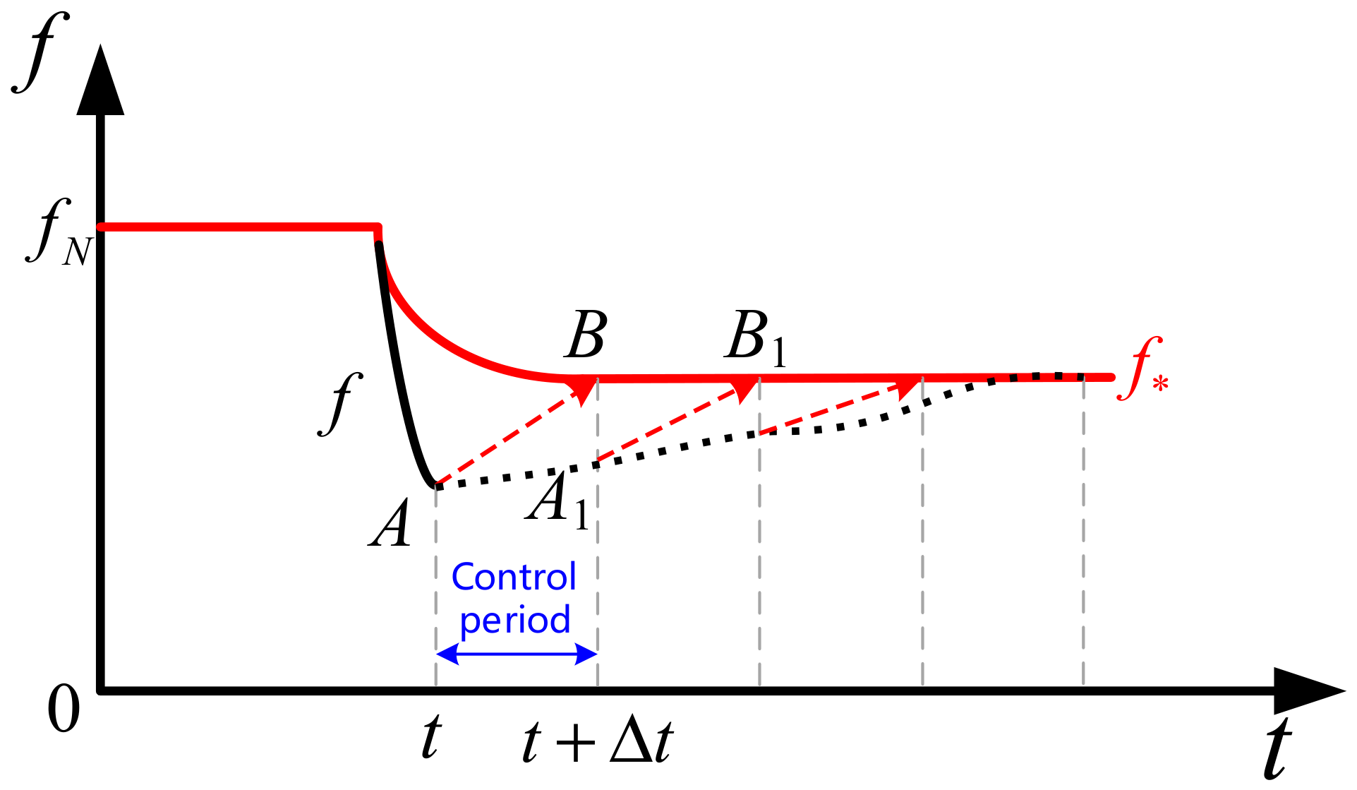
The control schematic of the proposed strategy within one control step is shown in the following figure. When the system frequency is detected to exceed the frequency regulation deadband, the sending-end OWFs controller generates the target frequency curve according to the method proposed in the previous section. For each control step, the deviation between the measured frequency fA at the beginning of the step and the target frequency fB at the end of the step is calculated. Then, based on the principle of coordination with SGs, the OWFs control command is calculated and issued. When the time advances to the next control step, the above calculation is performed again, and the frequency is eventually stabilized around the target frequency.
4.2. Calculation of Frequency Regulation Commands for Sending-End OWFs
4.2.1. Calculation of Total Regulation Power Demand
Combined with Figure 1 and Figure 8, to regulate the frequency from fA to fB, the total frequency regulation power demand within the control step is calculated as follows,
where ΔPtot,A→B denotes the total regulation power variation required to regulate the frequency from fA to fB within the control step. ΔPa,A and ΔPa,B denote the total regulation power at the beginning and ending instants of the control step, respectively. D is mainly affected by load damping and generally varies only slightly. H can be calculated from information such as the power capacities of OWFs and SGs as follows.
where HSG denotes the system inertia time constant when only SGs are included, SN,i is the rated capacity of SG i, Sw,j is the rated capacity of wind turbine j, and m and n denote the numbers of wind turbines and SGs, respectively. In Equation (20), the inertia term of SG is converted to the total system base according to the corresponding capacity ratio, so that the equivalent inertia is expressed on a unified per-unit basis. It should be noted that although wind turbines have physical rotor inertia, this inertia contributes to system frequency support only when active power support is provided. If such control is not implemented, the inertia of the wind turbines remains within the rotors and cannot provide net support to the power system. Moreover, the specific inertia contribution provided by wind power varies with the wind power control strategy. It is generally relatively small and difficult to quantify directly. Therefore, the wind power inertia is neglected in the above analysis.
Figure 8.
Schematic diagram of frequency tracking control within a control step.
4.2.2. Approximate Calculation of SG Support Power Variation
After the control target is determined, the mechanical power of SGs can be approximately calculated according to Equation (12). The mechanical power variation of SGs within the control step can be approximated as
where ΔPm,A→B denotes the mechanical power variation of SGs corresponding to regulating the frequency from fA to fB within the control step, and Δttrol is the control step.
4.2.3. Calculation of OWFs Frequency Regulation Power Command
The frequency is supported jointly by OWFs and SGs. Based on Equations (19) and (21), the calculation formula for the OWFs frequency regulation power variation can be obtained as
where ΔPw,A→B denotes the OWFs frequency regulation power command variation corresponding to regulating the frequency from fA to fB within the control step. Obviously, the OWFs frequency regulation command can be calculated only by measuring the system frequency and basic parameters. Furthermore, by adding the above term to the OWFs power at the initial instant of the control step, the OWFs frequency regulation power command within this step can be obtained as
where ΔPw,A and ΔPw,B denote the OWFs frequency regulation commands at the beginning and ending instants of the control step, respectively.
By solving the above steps within each control step, the frequency regulation power commands of the wind turbines in each control step can be calculated in a receding manner. The above control process inherently contains a coordinated control mechanism between wind turbines and SGs guided by the target frequency. Specifically, the total frequency regulation demand is first calculated according to the target frequency and the measured frequency within the control step. Then, considering that the response of SGs is much slower than that of wind turbines, the SG output power variation within the control step is approximately calculated. Finally, the difference between the two is taken as the wind turbine regulation power variation command within this step and is issued for execution.
4.3. Complete Implementation of the Control Strategy
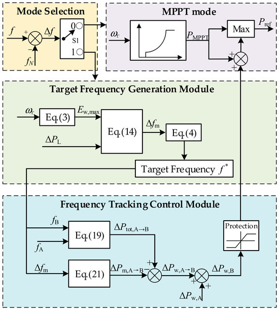
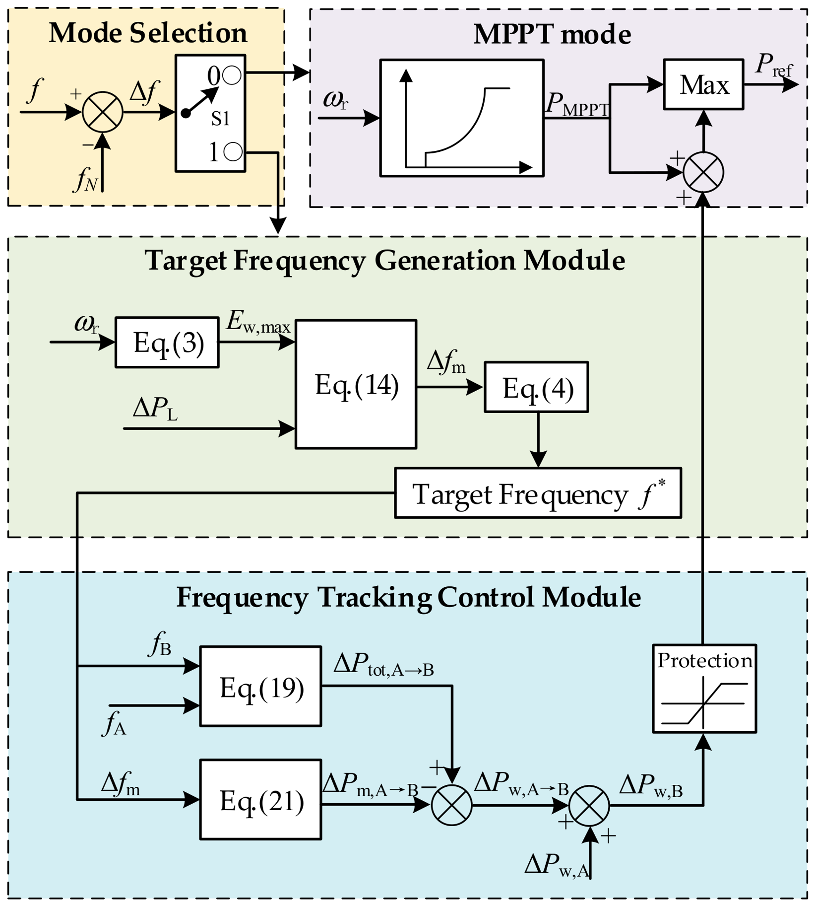
The complete implementation of the proposed strategy is shown in Figure 9. The mode selection module detects the system frequency deviation. When the system frequency deviation Δf is within the frequency regulation deadband, the selection module outputs 0, the controller operates in the MPPT mode, and the target frequency generation and tracking control modules are blocked. When Δf is detected to exceed the frequency regulation deadband, the selection module outputs 1. The target frequency generation module calculates the available rotor kinetic energy of the OWFs according to Equation (3), outputs the target frequency deviation according to Equation (14), and then sends it to Equation (4) to form the target frequency curve. After receiving the target frequency curve, the frequency tracking control module calculates Equations (19) and (21) and takes their difference to obtain the power command of the wind turbines within the control step, which is added to the original MPPT module to achieve tracking control. To ensure rotor speed safety, the proposed controller is equipped with a rotor speed protection module. Meanwhile, to ensure that the wind turbines can safely recover to their original operating state after providing frequency support, a frequency support exit strategy based on switching to MPPT control is adopted in this controller. This corresponds to the Max module before the reference power output in Figure 9. Specifically, when the output power of the wind turbines decreases to the MPPT power, the control mode is switched to MPPT control. Therefore, the actual duration of wind turbine participation in frequency control in this controller is determined by the intersection time between the MPPT power curve and the output electromagnetic power curve.
Figure 9.
Target frequency generation—dynamic tracking controller structure.
5. Case Study
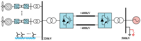
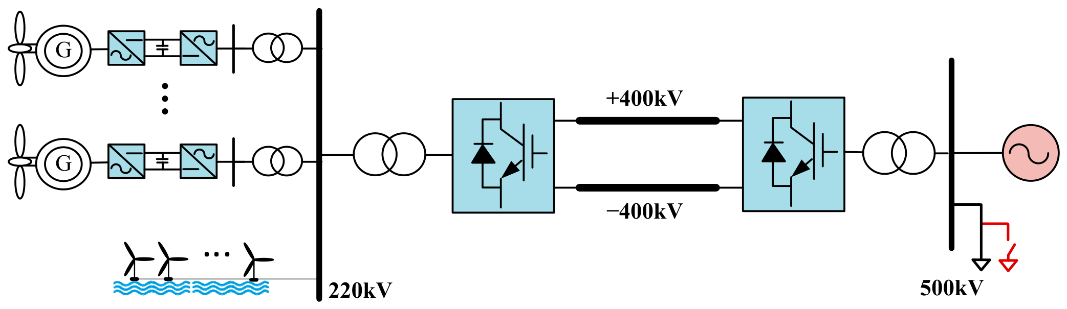
To verify the effectiveness of the proposed frequency control target design and tracking control strategy, the model shown in Figure 10 is built in MATLAB 2024b/Simulink for validation. The OWFs consist of 550 wind turbines, each with a rated capacity of 2 MW, and the corresponding wind speed range in the MPPT control stage is 6.5–9.5 m/s. Other detailed system model parameters are listed in Table 1. The calculated fourth-order fitting coefficients in Equation (16) are listed in Table 2.
Figure 10.
Simulation system structure diagram.
Table 1.
System model parameters.
Table 2.
Fourth-order fitting coefficients in Equation (16).
5.1. Effectiveness Verification of Frequency Control Target Design
To verify the effectiveness of the proposed frequency control target design method, the effectiveness of control target design under different wind speeds is examined. In each case, a sudden load increase of 300 MW is applied at t = 10.0 s.
5.1.1. Effectiveness Verification of Control Target Design at a Wind Speed of 9.0 m/s
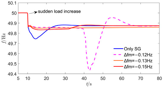
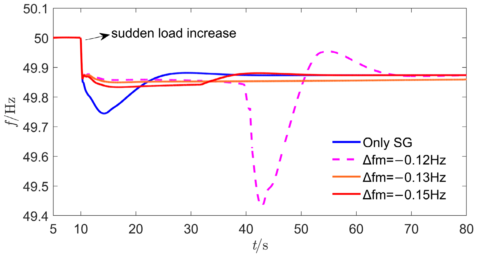
At a wind speed of 9.0 m/s, Δfm calculated by the proposed target frequency design method is −0.1250 Hz. When the target frequency deviation level is designed as −0.12 Hz, the frequency can be regulated around the designed value in the initial control stage. However, due to the excessive utilization of OWFs’ rotor kinetic energy, a relatively large secondary frequency drop occurs in the later stage. When the designed value is lower than the theoretical value, i.e., −0.13 Hz and −0.15 Hz, the measured frequency can be regulated around the target frequency, and no secondary frequency drop occurs. The results are shown in Figure 11.
Figure 11.
Frequency comparison under different control objectives at a wind speed of 9.0 m/s.
5.1.2. Effectiveness Verification of Control Target Design at a Wind Speed of 7.5 m/s
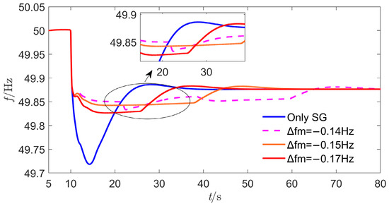
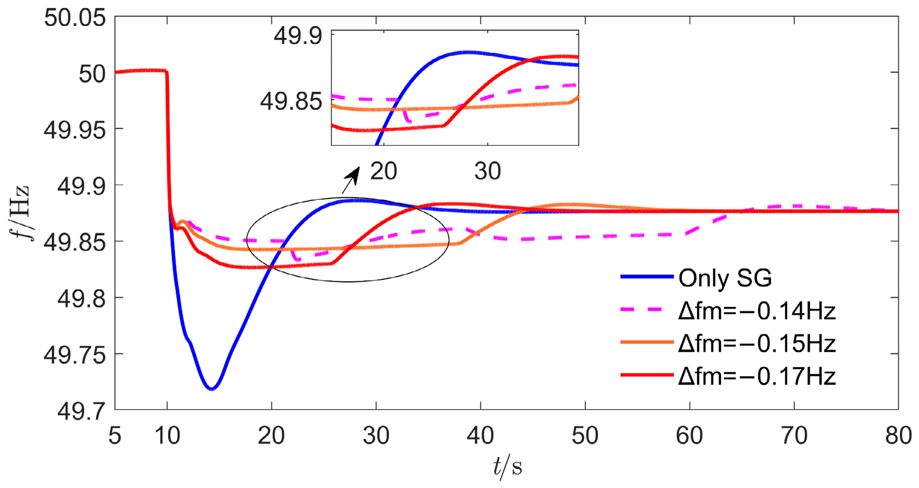
At a wind speed of 7.5 m/s, Δfm calculated by the proposed target frequency design method is −0.1413 Hz. It can also be observed from Figure 12 that when the designed target frequency deviation level, i.e., −0.14 Hz, is higher than the theoretical maximum value, a secondary frequency drop occurs, but its magnitude is much smaller than that at the wind speed of 9 m/s. When the designed target frequency is lower than the theoretical maximum value, no secondary frequency drop occurs.
Figure 12.
Frequency comparison under different control objectives at a wind speed of 7.5 m/s.
5.1.3. Verification of the Effectiveness of the ts Selection in Control Target Design
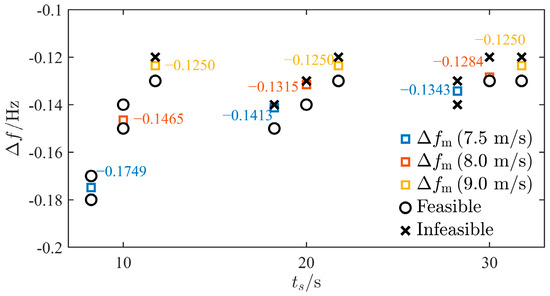
When formulating the target frequency based on Equation (14), the classical effective frequency regulation time ts =20 s is adopted. To demonstrate the validity of this choice, and considering common inertia and primary frequency regulation events, ts =10 s, 20 s, and 30 s are selected, respectively, to analyze the feasibility of the tuned control target under different wind speeds. The results are shown in Figure 13.
Figure 13.
Simulation results of control target feasibility under different wind speeds and different values of ts.
When the wind speed is 9.0 m/s, the target frequency deviation level under all three values of ts is −0.1250 Hz, indicating the case of larger OWFs frequency-regulation energy shown by the blue curve in Figure 3. In other words, the tuned target frequency is not affected by the choice of ts. When the wind speed is 7.5 m/s or 8.0 m/s, the tuned values differ for different ts, corresponding to the case of smaller OWFs frequency-regulation energy. The details are as follows. When ts = 10 s, the tuned target frequency deviation is −0.1749 Hz at a wind speed of 7.5 m/s. However, the actual target frequency can still be achieved even when it is higher than this value. A similar conclusion holds for a wind speed of 8.0 m/s. This indicates that the target frequency tuning with ts = 10 s is relatively conservative, which is not conducive to improving the frequency regulation performance. When ts = 30 s, there are cases where the actual target frequency cannot be achieved even when it is lower than the tuned value at a wind speed of 7.5 m/s. This indicates that the target frequency tuning is too aggressive. Combined with Figure 3, a larger ts leads to a higher target frequency, which may exceed the capability of the OWFs themselves and may even cause a secondary frequency drop. When ts = 20 s, the tuned target frequency under various wind speeds ensures that the actual target frequency can be achieved when it is lower than the tuned value, whereas it is difficult to achieve when it is higher than the tuned value. This choice balances the feasibility of the target frequency and the frequency improvement performance.
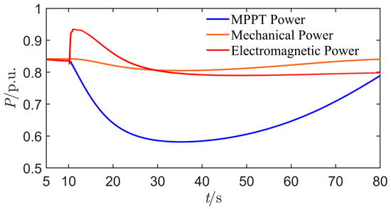
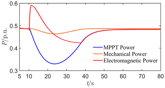
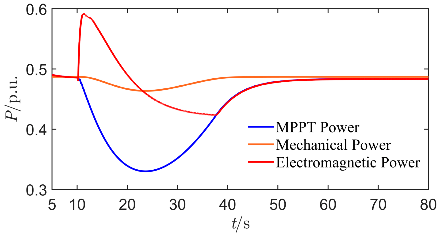
Furthermore, the OWFs power curves for the case of a wind speed of 9.0 m/s and Δfm = −0.13 Hz in Section 5.1.1, as well as for the case of a wind speed of 7.5 m/s and Δfm = −0.15 Hz in Section 5.1.2, are presented below to demonstrate the ts data used in the actual simulation, as shown in Figure 14 and Figure 15.
Figure 14.
OWFs power curve at a wind speed of 9.0 m/s and Δfm = −0.13 Hz.
Figure 15.
OWFs power curve at a wind speed of 7.5 m/s and Δfm = −0.15 Hz.
It can be observed that, at a wind speed of 9.0 m/s, the simulation results indicate that the actual ts is approximately 20 s, whereas at a wind speed of 7.5 m/s, the actual ts is approximately 15 s. Considering that ts is used only to obtain a reasonable tuning value for the target frequency level, it is not required to be exactly the same as the actual ts, which is difficult to achieve in practice. Together with Figure 13, these results indicate that the typical value of 20 s adopted in this paper has a practical reference value. Meanwhile, the tuned value of ts does not vary with wind speed. Its tuned value should have a certain degree of generality for wind speeds in the MPPT stage.
It should be noted that the actual ending time of OWFs participation in frequency regulation is determined by the intersection between the electromagnetic power and the MPPT power. This duration is longer than the effective frequency regulation time. Therefore, the actual ts cannot be analyzed based on the duration for which the frequency curve remains at the target level, since they are two completely different concepts.
5.1.4. Verification of the Effectiveness of the Target-Trajectory Time Constant
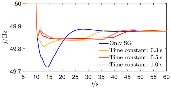
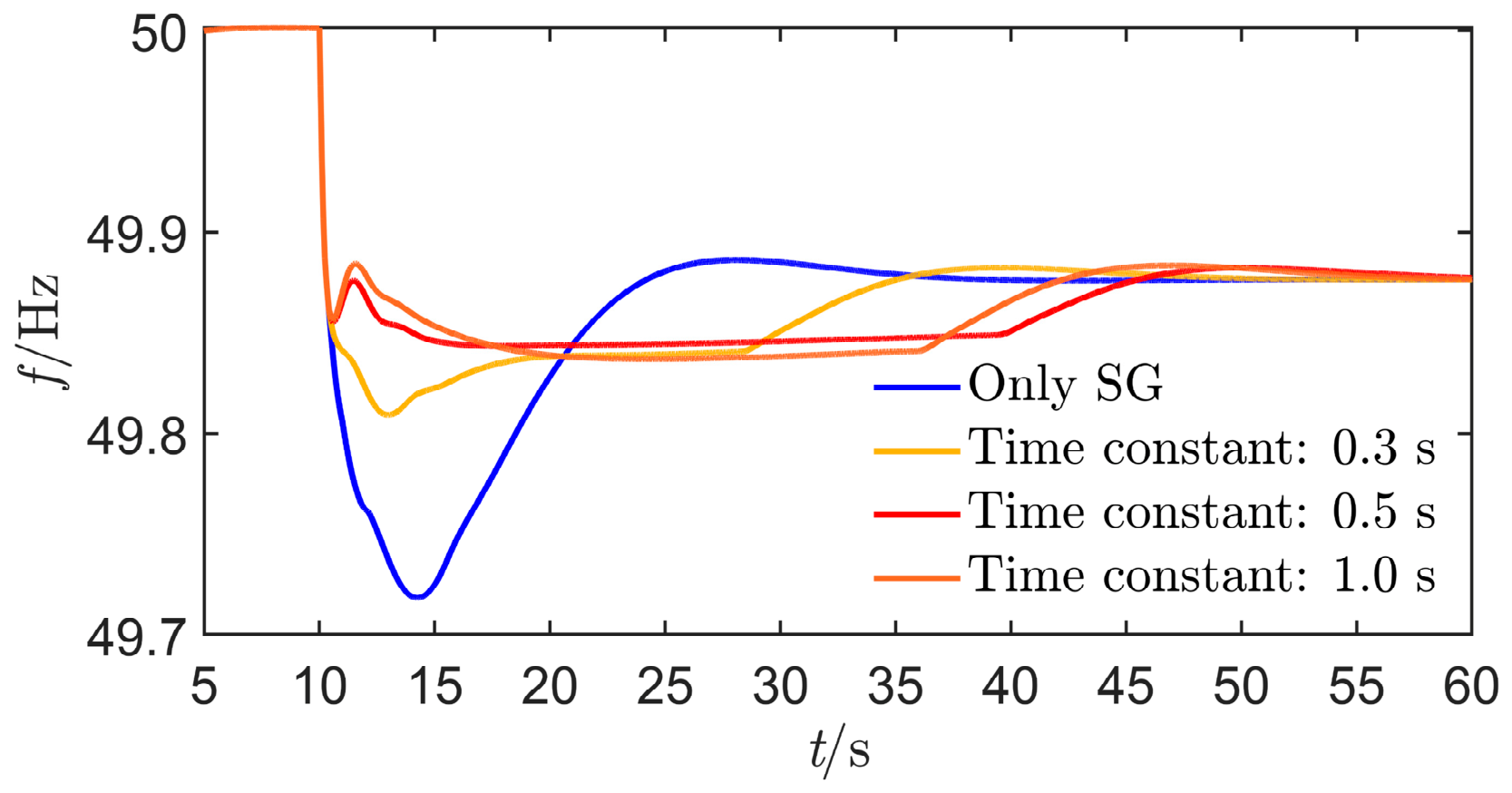
In the above simulation verification, the time constant of the target frequency is empirically set to 0.5 s. To further illustrate the control performance under different time constants, comparative simulations are also conducted at a wind speed of 7.5 m/s, where the time constants are set to 0.3 s, 0.5 s, and 1.0 s, respectively. The simulation comparison results are shown in Figure 16.
Figure 16.
Frequency control performance under different target-trajectory time constants.
It can be seen that the difference in the target-trajectory time constant mainly affects the frequency dynamics in the initial control stage, while it has little influence on the quasi-steady-state frequency. Specifically, a shorter time constant leads to a lower initial frequency and a lower frequency level, and the OWFs exit frequency regulation relatively earlier. However, under common values of the time constant, the frequency support effect can still be achieved.
5.2. Effectiveness Verification of the Control Strategy
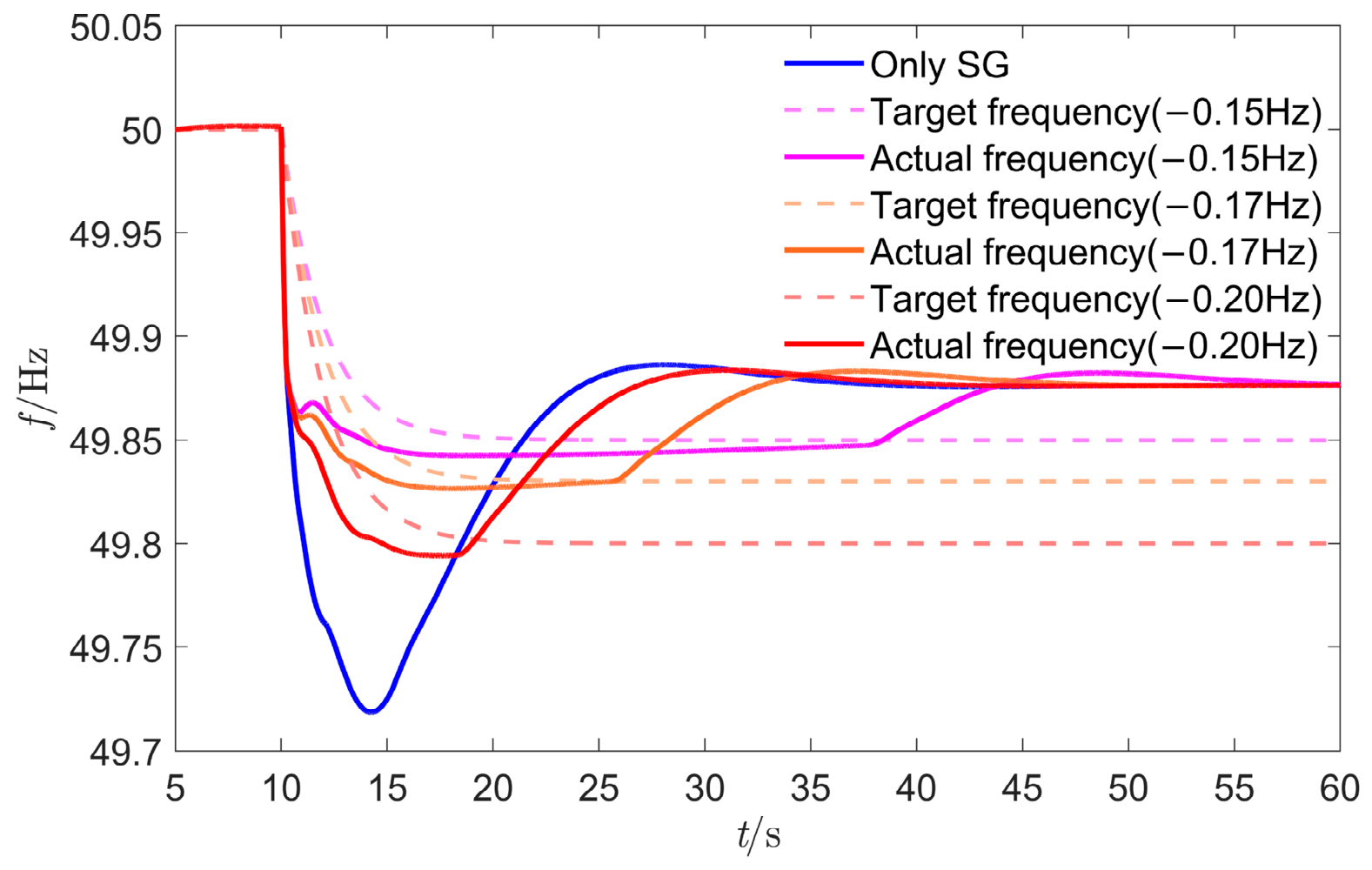
To verify the effectiveness of the proposed control strategy in frequency tracking control, the case with a wind speed of 7.5 m/s is analyzed as an example. According to Section 3.2 and Section 5.1.2, Δfm at this wind speed is −0.1413 Hz. Therefore, Δfm is set to −0.20 Hz, −0.17 Hz and −0.15 Hz, respectively. The frequency tracking control performance is shown in Figure 17.
Figure 17.
Frequency tracking performance at different target frequencies.
As shown in Figure 17, in the initial stage after the disturbance event occurs, the frequency drops rapidly to activate the regulation potential of SGs. Subsequently, guided by the control target, the actual frequency curve gradually approaches the target frequency curve. Meanwhile, the frequency tracking error is relatively large in the early control stage and gradually decreases as the control strategy is executed step by step. To quantitatively analyze the tracking control performance, the maximum tracking error emax and the average tracking error eavg are defined as follows.
where tini denotes the starting time for error calculation. To eliminate the influence of the rapid frequency drop stage on the evaluation indices, tini is set to the time instant 5.0 s after the disturbance occurs in this paper. tend is the ending time for error calculation, corresponding to the ending time of OWFs participation in frequency regulation, i.e., the time instant when the frequency in the above figure begins to transition to the steady-state value.
The average tracking error is calculated by sampling every 0.1 s over the sampling interval [tini, tend], where N denotes the total number of samples. The tracking error percentage is defined as the ratio of the tracking error to the target frequency deviation level. Table 3 gives the calculated tracking errors under different target frequencies.
Table 3.
Tracking error at different target frequencies.
Under different target frequencies, the maximum tracking error is approximately 7.0–11.0%, and the average tracking error is approximately 1–5%. Considering that the measured frequency gradually approaches the target frequency in the later stage of tracking control, the effectiveness of the proposed strategy in tracking the target frequency is demonstrated.
5.3. Superiority Verification of the Target Design-Tracking Control Scheme
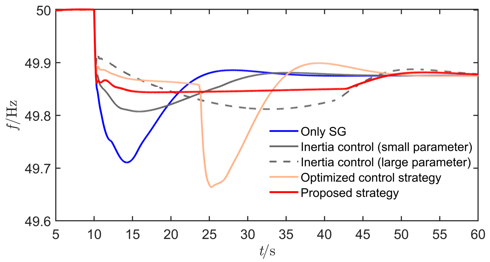
To demonstrate the superiority of the proposed strategy, comparisons are conducted with the cases of no OWF frequency support, synthetic inertia control with large and small parameters, and an existing optimal control strategy. For all strategies, the wind speed is set to 8.0 m/s, and a sudden load increase of 300 MW is applied at t = 10.0 s. In the simulation of the optimal control strategy, the proportional factor between the frequency nadir and the quasi-steady-state frequency calculated from the nonlinear binary equation is 1.201. The simulation results are shown in Figure 18.
Figure 18.
Comparison of frequency control performance under different control strategies.
In terms of frequency improvement, the frequency support performance of synthetic inertia control differs significantly with different control parameter settings, while its improvement of the frequency nadir is limited. Although the optimal control strategy can support the frequency nadir to a higher value in the initial control stage, the calculated parameters are relatively idealized because the wind energy capture loss is ignored. As a result, rotor speed protection is triggered, leading to a relatively large secondary frequency drop. Overall, the proposed strategy achieves the best global frequency improvement performance.
To further objectively reflect the control performance of the above methods, the quantitative results are provided in Table 4.
Table 4.
Quantitative comparison results of different methods.
It can be seen that the proposed method achieves the highest frequency nadir. Although the differences in the rate of change of frequency among the various methods are not significant, the traditional optimal control method exhibits a relatively large rate of change of frequency due to the secondary frequency drop. Regarding the minimum rotor speed, the synchronous generator support method does not involve OWF participation in frequency regulation, so the minimum rotor speed is actually equal to the MPPT operating speed. Under the inertia control strategy, a larger control parameter results in a lower rotor speed and less OWFs energy consumption; however, its frequency support performance is weaker than that of the proposed method. In contrast, the proposed method achieves the best control performance while consuming relatively little energy, which demonstrates its effectiveness.
It should be noted that there is no computational time for the first three methods. For the traditional optimal control algorithm and the proposed method, the calculations are simple numerical computations and can be completed almost instantaneously. Therefore, computational time is not compared in the table above, and this does not affect the validity of the proposed method.
5.4. Robustness Verification of the Control Strategy
The implementation of the proposed strategy requires the system equivalent inertia time constant H, damping coefficient D, and power disturbance ΔPL. However, their accurate values are often difficult to obtain in practical power grids. In addition, communication delays inevitably exist in frequency measurement and control command transmission for OWFs integrated via MMC-HVDC. Therefore, it is necessary to demonstrate the robustness of the proposed strategy against parameter acquisition errors, power disturbance sensing errors, and communication delays. The case with a wind speed of 7.5 m/s and a sudden load increase of 300 MW at t = 10.0 s is analyzed as an example.
5.4.1. Robustness Against Parameter Acquisition Errors
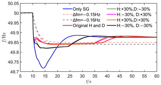
The estimation errors of H and D are set within the range of ±30%, respectively, and the corresponding frequency control performance is shown in Figure 19.
Figure 19.
Robustness of the proposed strategy under parameter uncertainties.
It can be observed that when the original values of H and D are used, when H is underestimated by 30% and D is overestimated by 30%, when H is overestimated by 30% and D is overestimated by 30%, the target frequency deviation level is −0.15 Hz in all three cases. In these cases, the actual frequency can be regulated around the target frequency by the controller, and no significant difference in control performance is observed. When H is overestimated by 30% and D is underestimated by 30%, and when H is underestimated by 30% and D is underestimated by 30%, the target frequency deviation level is −0.16 Hz in both cases. The corresponding controller can also regulate the actual frequency around the target frequency. In summary, the proposed strategy exhibits a certain degree of robustness against acquisition errors in H and D.
5.4.2. Robustness Against Communication Delays
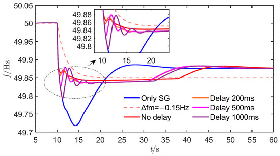
Considering that the control step of the controller is 150 ms, communication delays of 200 ms, 500 ms, and 1000 ms are set, respectively, to verify robustness. The corresponding frequency control results are shown in Figure 20.
Figure 20.
Robustness of the proposed strategy against communication delays.
Overall, an increase in communication delay leads to certain frequency fluctuations within the first 2–5 s of the control process, and a larger delay results in more significant frequency fluctuations. Under a delay of 1000 ms, the maximum fluctuation range does not exceed 0.08 Hz. Subsequently, the frequency behaves similarly to the case without delay, steadily approaching the target frequency. Overall, the proposed strategy exhibits a certain degree of robustness against communication delays.
5.4.3. Robustness Against Power Disturbance Estimation Errors
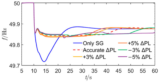
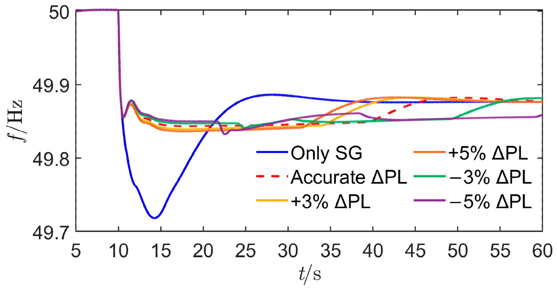
Considering the disturbance estimation accuracy reported in existing studies [26,27], the sensed disturbance is assumed to deviate from the actual disturbance by 3% and 5%, respectively, to analyze the effectiveness of the proposed control target design method and frequency control method. The corresponding frequency control results are presented in Figure 21.
Figure 21.
Robustness of the proposed strategy against power disturbance estimation errors.
It can be seen that overestimation of the power disturbance leads to a lower tuned target frequency. In this case, the controller can still achieve tracking control, and the effectiveness of the proposed strategy is not affected, indicating that the proposed method has good robustness against power disturbance overestimation. When the estimated power disturbance is smaller than the actual value, the tuned target frequency becomes higher. In this case, the controller can basically still achieve tracking control, but a slight frequency drop may occur in the later stage due to insufficient OWFs energy. This, in turn, shows that the proposed target-frequency tuning method can well reflect the actual frequency support capability of the OWFs. At the same time, it also indicates that the robustness against power disturbance underestimation is relatively weaker. This issue can be addressed by improving the accuracy of disturbance estimation or by multiplying the target-frequency tuning result by a conservative coefficient. This will also be one of the authors’ future research directions.
6. Conclusions
This paper proposes an optimized frequency trajectory level design method based on the available rotor kinetic energy of OWFs, as well as a target frequency tracking control strategy intended to coordinate the outputs of OWFs and SGs. The following conclusions are drawn.
In islanded power grids or future power grids with a high proportion of renewable energy, a promising idea can be explored, namely, “determining the expected target frequency dynamics according to the available energy of renewable energy sources and then designing the control strategy in reverse according to the target frequency dynamics.” Focusing on OWFs integrated via MMC-HVDC, this paper analyzes the general characteristics of the proportion of effective frequency regulation energy to released rotor kinetic energy of the sending-end OWFs. On this basis, the quantitative relationship between the optimized frequency trajectory level at the receiving end and the frequency regulation energy of the sending-end OWFs is derived, forming a target frequency design method.
According to the designed target frequency, a discrete tracking control method can be adopted to ensure coordinated output regulation between OWFs and SGs. Within each control step, the total frequency regulation demand, approximate SG support power, and OWFs frequency regulation command are calculated, and frequency tracking is achieved through receding execution. Simulations verify that the average tracking error of the proposed strategy is approximately 5%, and that the proposed strategy exhibits a certain degree of robustness against parameter acquisition errors and communication delays.
Although the proposed method has been verified through simulations, further work is still needed to improve its practical applicability. Future research will focus on experimental verification, real-time dynamic estimation of key parameters, and optimized allocation of control commands among multiple wind turbines within the OWFs while considering wake effects.
Author Contributions
Conceptualization, Y.Z. and D.C.; methodology, Y.Z.; software, Q.H.; validation, Y.Z., Z.H. and H.W.; formal analysis, Y.Z.; investigation, D.C.; resources, Q.H.; data curation, D.C.; writing—original draft preparation, Y.Z.; writing—review and editing, Y.Z.; visualization, Y.Z.; supervision, D.C.; project administration, D.C.; funding acquisition, Q.H. All authors have read and agreed to the published version of the manuscript.
Funding
This research was funded by the Science and Technology Project of SGCC (Research on Frequency Active Support Collaborative Optimization Control Technology for Offshore Wind Power Transmission through VSC-HVDC) (52110425001F-021-ZN).
Institutional Review Board Statement
Not applicable.
Informed Consent Statement
Not applicable.
Data Availability Statement
The original contributions presented in this study are included in the article. Further inquiries can be directed to the corresponding author.
Conflicts of Interest
The authors declare no conflicts of interest. The authors declare that this study received funding from the Science and Technology Project of SGCC. The funder had the following involvement with the study: study design.
Abbreviations
The following abbreviations are used in this manuscript:
| OWFs | Offshore wind farms |
| MMC-HVDC | Modular multilevel converter-based high-voltage direct current |
| SG | Synchronous generator |
| MPPT | Maximum power point tracking |
References
- Normandia Lourenço, L.F.; Louni, A.; Damm, G.; Netto, M.; Drissi-Habti, M.; Grillo, S.; Sguarezi Filho, A.J.; Meegahapola, L. A Review on Multi-Terminal High Voltage Direct Current Networks for Wind Power Integration. Energies 2022, 15, 9016. [Google Scholar] [CrossRef] [Scilit]
- Yan, K.; Li, G.; Zhang, R.; Xu, Y.; Jiang, T.; Li, X. Frequency Control and Optimal Operation of Low-Inertia Power Systems with HVDC and Renewable Energy: A Review. IEEE Trans. Power Syst. 2024, 39, 4279–4295. [Google Scholar] [CrossRef] [Scilit]
- Wu, D.; Seo, G.-S.; Xu, L.; Su, C.; Kocewiak, L.; Sun, Y.; Qin, Z. Grid Integration of Offshore Wind Power: Standards, Control, Power Quality and Transmission. IEEE Open J. Power Electron. 2024, 5, 583–604. [Google Scholar] [CrossRef] [Scilit]
- Hao, J.; Zheng, H.; Cheng, X.; Li, Y.; Bo, L.; Wei, J. Optimal Control Strategy and Evaluation Framework for Frequency Response of Combined Wind–Storage Systems. Technologies 2025, 13, 259. [Google Scholar] [CrossRef] [Scilit]
- Sun, K.; Zhou, H.; Yao, W.; Xiao, B.; Wen, J. Comprehensive Control of MMC-HVDC Integrated Offshore Wind Farm System Including Optimized Energy Control for Fast Frequency Support. J. Mod. Power Syst. Clean Energy 2025, 13, 1966–1979. [Google Scholar] [CrossRef] [Scilit]
- Xu, D.; Li, H.; Yang, X.; Yang, H.; Yang, H.; Bai, Z. Cooperative Operation of P2G-Based Multi-Energy Systems Considering Proactive Demand Response of Energy-Intensive Multi-Process Industrial Loads. IEEE Trans. Ind. Appl. 2025, 1–13. [Google Scholar] [CrossRef] [Scilit]
- Zhang, C.; Yang, X.; Ding, L.; Yang, Y.; Li, H.; Yang, Z.; Wu, Q.; Wen, J. Design of Flexible DC-SOP Toward Four-Quadrant Power Flow Control in Bipolar Distribution Networks. IEEE Trans. Smart Grid 2026, 17, 2614–2617. [Google Scholar] [CrossRef] [Scilit]
- Fu, X.; Ma, L.; Ge, H.; Zhang, J. Security Analysis of Agricultural Energy Internet Considering Electricity Load Control for Dragon Fruit Cultivation. Inf. Process. Agric. 2025, 12, 27–39. [Google Scholar] [CrossRef] [Scilit]
- Gao, H.; Zhang, F.; Ding, L.; Cornélusse, B.; Zhang, G.; Salimu, A. Multi-Segment Droop Control and Optimal Parameter Setting Strategy of Wind Turbine for Frequency Regulation. Int. J. Electr. Power Energy Syst. 2024, 158, 109968. [Google Scholar] [CrossRef] [Scilit]
- Gao, H.; Zhang, F.; Ding, L.; Zhang, G.; Yang, L.; Salimu, A. Towards Non-Virtual Inertia Control of Renewable Energy for Frequency Regulation: Modeling, Analysis and New Control Scheme. Int. J. Electr. Power Energy Syst. 2024, 162, 110314. [Google Scholar] [CrossRef] [Scilit]
- Jiang, C.; Cai, G.; Yang, D.; Liu, X.; Hao, S.; Li, B. Multi-Objective Configuration and Evaluation of Dynamic Virtual Inertia from DFIG Based Wind Farm for Frequency Regulation. Int. J. Electr. Power Energy Syst. 2024, 158, 109956. [Google Scholar] [CrossRef] [Scilit]
- Loza, B.; Minchala, L.I.; Ochoa-Correa, D.; Arévalo-Cordero, P. An Adaptive Inertial Control Strategy for Wind Turbines via Fuzzy Logic and OPPTE Integration. Technologies 2025, 13, 547. [Google Scholar] [CrossRef] [Scilit]
- Kheshti, M.; Ding, L.; Bao, W.; Yin, M.; Wu, Q.; Terzija, V. Toward Intelligent Inertial Frequency Participation of Wind Farms for the Grid Frequency Control. IEEE Trans. Ind. Inform. 2020, 16, 6772–6786. [Google Scholar] [CrossRef] [Scilit]
- Bao, W.; Ding, L.; Liu, Z.; Zhu, G.; Kheshti, M.; Wu, Q.; Terzija, V. Analytically Derived Fixed Termination Time for Stepwise Inertial Control of Wind Turbines—Part I: Analytical Derivation. Int. J. Electr. Power Energy Syst. 2020, 121, 106120. [Google Scholar] [CrossRef] [Scilit]
- Guo, Y.; Bao, W.; Ding, L.; Liu, Z.; Kheshti, M.; Wu, Q.; Terzija, V. Analytically Derived Fixed Termination Time for Stepwise Inertial Control of Wind Turbines—Part II: Application Strategy. Int. J. Electr. Power Energy Syst. 2020, 121, 106106. [Google Scholar] [CrossRef] [Scilit]
- Li, C.; Yang, Y.; Mao, X.; Xiong, X.; Dragicevic, T. Modeling, Control and Stabilization of Virtual Synchronous Generator in Future Power Electronics-Dominated Power Systems: A Survey of Challenges, Advances, and Future Trends. Int. J. Electr. Power Energy Syst. 2025, 171, 111001. [Google Scholar] [CrossRef] [Scilit]
- Jiang, Y.; Cohn, E.; Vorobev, P.; Mallada, E. Storage-Based Frequency Shaping Control. IEEE Trans. Power Syst. 2021, 36, 5006–5019. [Google Scholar] [CrossRef] [Scilit]
- Xiong, L.; Liu, L.; Liu, X.; Liu, Y. Frequency Trajectory Planning Based Strategy for Improving Frequency Stability of Droop-Controlled Inverter Based Standalone Power Systems. IEEE J. Emerg. Sel. Top. Circuits Syst. 2021, 11, 176–187. [Google Scholar] [CrossRef] [Scilit]
- Sun, M.; Min, Y.; Xiong, X.; Chen, L.; Zhao, L.; Feng, Y.; Wang, B. Practical Realization of Optimal Auxiliary Frequency Control Strategy of Wind Turbine Generator. J. Mod. Power Syst. Clean Energy 2022, 10, 617–626. [Google Scholar] [CrossRef] [Scilit]
- Sun, M.; Sun, Y.; Chen, L.; Zou, Z.; Min, Y.; Liu, R.; Xu, F.; Wu, Y. Novel Temporary Frequency Support Control Strategy of Wind Turbine Generator Considering Coordination with Synchronous Generator. IEEE Trans. Sustain. Energy 2022, 13, 1011–1020. [Google Scholar] [CrossRef] [Scilit]
- Zhang, Y.; Hao, Z.; Yang, S.; Zhang, B. A System-View Optimal Additional Active Power Control of Wind Turbines for Grid Frequency Support. IEEE Trans. Power Syst. 2024, 39, 4323–4335. [Google Scholar] [CrossRef] [Scilit]
- Zhang, Y.; Yang, S.; Hao, Z.; Zhang, B. Model-Free Fast Frequency Support of Wind Farms for Tracking Optimal Frequency Trajectory. IEEE Trans. Sustain. Energy 2024, 15, 2638–2650. [Google Scholar] [CrossRef] [Scilit]
- Zhang, C.; Sun, X.; Cai, D.; Ding, L.; Bao, W.; Ma, R.; Terzija, V. Delayed Inertial Control-Based Coordinated Frequency Support Using Wind Turbine Generators. Int. J. Electr. Power Energy Syst. 2025, 171, 111025. [Google Scholar] [CrossRef] [Scilit]
- Anderson, P.M.; Mirheydar, M. A Low-Order System Frequency Response Model. IEEE Trans. Power Syst. 1990, 5, 720–729. [Google Scholar] [CrossRef] [Scilit]
- Wang, S.; Tomsovic, K. A Novel Active Power Control Framework for Wind Turbine Generators to Improve Frequency Response. IEEE Trans. Power Syst. 2018, 33, 6579–6589. [Google Scholar] [CrossRef] [Scilit]
- Wang, W.; Yi, N.; Cai, Y.; Cao, Y.; Li, Z.; Quan, S. A Power-Disturbance Observer-based Auxiliary Frequency Control of Grid-forming VSC-HVDC Systems. Proc. CSEE 2025, 45, 1680–1691. [Google Scholar] [CrossRef]
- Yang, F.; Shao, X.; Muyeen, S.M.; Li, D.; Lin, S.; Fang, C. Disturbance Observer Based Fractional-Order Integral Sliding Mode Frequency Control Strategy for Interconnected Power System. IEEE Trans. Power Syst. 2021, 36, 5922–5932. [Google Scholar] [CrossRef] [Scilit]

Disclaimer/Publisher’s Note: The statements, opinions and data contained in all publications are solely those of the individual author(s) and contributor(s) and not of MDPI and/or the editor(s). MDPI and/or the editor(s) disclaim responsibility for any injury to people or property resulting from any ideas, methods, instructions or products referred to in the content. |
© 2026 by the authors. Licensee MDPI, Basel, Switzerland. This article is an open access article distributed under the terms and conditions of the Creative Commons Attribution (CC BY) license.