Anomaly Score-Based Cross-Machine Wind Turbine Component Diagnosis: A Case Study and Benchmark

Abstract

Reliable wind turbine component diagnosis requires cross-machine knowledge transfer since verified fault cases are rare. However, coarse fault interval annotations and turbine-specific operating behavior make this transfer difficult. This paper introduces a benchmark framework for cross-machine wind turbine component diagnosis on a new industrial dataset derived from Supervisory Control and Data Acquisition (SCADA) and vibration-derived kinematics data. The dataset is publicly available upon request and contains anomaly score-based embeddings. These embeddings are feature vectors whose entries quantify how strongly signals or component-related features deviate from learned normal behavior. The benchmark compares classical machine learning models, deep learning models, adversarial domain adaptation variants, and a simple baseline. Hyperparameter selection is performed without target labels using source classification loss, target prediction entropy, or Soft Neighborhood Density (SND). Our experiments show that, in the SCADA validation stage, source classification loss achieves the highest mean case diagnosis score among the evaluated objectives. In our evaluation, simple baselines remain highly competitive. The SCADA component score baseline achieves the highest test case diagnosis accuracy, while an ensemble of one-class support vector machines achieves the highest kinematics test case diagnosis accuracy. These findings indicate that anomaly score-based embeddings provide a useful representation for real-world component diagnosis, but that the small number of verified cases, coarse fault interval annotations, and partial label space mismatch remain major obstacles for reliable cross-machine adaptation.

1. Introduction

Wind energy is a central component of renewable electricity production, and the economic value of wind farms depends strongly on technical availability and maintenance efficiency [1,2]. Condition monitoring and predictive maintenance aim to reduce unplanned downtime by detecting abnormal behavior early and supporting timely maintenance decisions [2,3]. In operational wind turbine monitoring, however, the relevant question after an alarm or abnormal interval is often not only whether a turbine behaves anomalously, but which component is affected. This paper therefore focuses on component diagnosis: given a candidate fault interval, predict the affected turbine component.

Machine learning methods are widely used for wind turbine fault detection and diagnosis because they can learn discriminative representations from Supervisory Control and Data Acquisition (SCADA), vibration, or other condition-monitoring data [3,4,5]. Their practical use is limited by cross-machine generalization. Signal distributions vary with turbine hardware, sensor configuration, control behavior, operating conditions, and environment, which creates source–target domain shifts between turbines and fault cases [6,7,8]. Fault cases are manually documented fault intervals with information about affected components. They are rare, imbalanced, and expensive to label [9,10,11]. The combination of domain shift and scarce labels makes it difficult to train a separate supervised model for every turbine, component, and operating regime.

Transfer learning and domain adaptation address this problem by reusing information from one or more source domains for a related target domain [12]. Parameter-based transfer learning commonly starts from a pretrained model and fine-tunes selected parameters on labeled target data. This strategy has been used for cross-working condition diagnosis of gearboxes, bearings, and wind turbine data, for example by fine-tuning ImageNet-pretrained convolutional models or by adapting models pretrained on source turbines [13,14,15]. Such approaches can be effective when a small labeled target set is available, but they do not match the setting considered here: when a new target fault case is diagnosed, its component label is not available for training or hyperparameter selection.

Unsupervised domain adaptation relaxes this requirement by using labeled source data together with unlabeled target data [16]. Feature-based methods reduce source–target discrepancy by minimizing distances such as maximum mean discrepancy or Wasserstein distance, or by learning domain-invariant representations through adversarial training [17]. Instance-based methods instead reweight source samples to reduce the effect of dissimilar or misleading source data in order to mitigate negative transfer. Both ideas are common in fault-diagnosis research, including bearing, gearbox, and wind turbine studies under varying working conditions [18,19,20,21,22,23,24].

Many domain adaptation methods assume a closed label space, meaning that the source and target domains contain the same fault classes. Real wind turbine diagnosis often violates this assumption. A target case usually corresponds to one unknown affected component, while the source pool may contain many additional component labels that are irrelevant to the target case. Partial domain adaptation addresses this label space mismatch by allowing the target label space to be a subset of the source label space and by reducing the influence of source-only outlier classes [25,26,27]. Multi-source domain adaptation further considers that source data may come from multiple machines or operating regimes with different relevance to the target task [28,29]. Recent work has also studied combinations of multi-source and partial adaptation for machinery fault diagnosis [30,31,32].

Anomaly score-based representations are widely used in condition monitoring as detection signals or as evidence for fault localization. An anomaly score is a numerical value that indicates how strongly a signal or feature deviates from learned normal behavior. In multivariate time-series diagnosis, channel-wise anomaly scores or reconstruction errors are often ranked over known anomalous intervals to identify responsible variables or sensor channels [33]. In industrial fault localization, per-sensor reconstruction errors can also be combined with expert knowledge to identify affected subsystems [34]. In wind turbine monitoring, however, such anomaly evidence is more commonly used for detection or explanation than as input data for cross-machine component diagnosis models. The present work therefore evaluates whether anomaly score-based embeddings, defined here as vectors of anomaly score features for each observation, can support case-level component diagnosis under target label-free model selection.

Despite progress in transfer learning and anomaly-based monitoring, realistic wind turbine component diagnosis remains underexplored. Many studies use laboratory machinery, simulated faults, closed label spaces, random window-level splits, or target labels for fine-tuning and model selection. These assumptions can overestimate performance in operational deployment. A credible benchmark must account for limited verified cases, coarse fault interval annotations, partial label space mismatch, and the absence of target component labels during hyperparameter optimization (HPO). In addition, it should compare domain adaptation models against strong simple baselines, because component-oriented anomaly representations may already encode much of the information needed for cross-machine component diagnosis.

This study presents a real-world benchmark for cross-machine wind turbine component diagnosis using anomaly score-based embeddings derived from industrial SCADA and vibration-derived kinematics data provided by Energie Baden-Württemberg AG (EnBW) [35]. The kinematics data are frequency-domain features derived from vibration spectra and drivetrain component frequency information, as described in Section 2. The resulting embedding space is referred to as the anomaly space in the remainder of the paper. The model that produces these embeddings, referred to as denoiser, first quantifies deviations from learned normal behavior and then represents each observation in this anomaly space. This paper uses the resulting anomaly score-based embeddings as input features for cross-machine component diagnosis.

This benchmark builds on our earlier supervised transfer learning study, which used an earlier anomaly space representation assembled mostly from hand-crafted features, threshold detections, and expert rules for wind turbine fault diagnosis, but focused on supervised classifiers rather than the target label-free model selection and domain adaptation setting evaluated here [36].

The main contributions of this work are summarized as follows:

• We introduce a real-world benchmark framework that combines anomaly score-based representations, partial domain adaptation, target label-free HPO, and case-based cross-machine evaluation for wind turbine component diagnosis.
• We define a unit-aware source–target split strategy in which each target case is held out, target labels are hidden during training and hyperparameter optimization, and same-unit source rows are excluded.
• We compare classical, one-class, neural, and adversarial adaptation models under realistic constraints: limited verified cases, coarse fault interval annotations, and partial label space mismatch.
• We systematically evaluate target label-free hyperparameter-selection objectives that use source labels and unlabeled target data without accessing target component labels.
• We show empirically that simple component-oriented baselines remain highly competitive against neural and domain adaptation models.

The remainder of this paper is organized as follows. Section 2 defines the task of component diagnosis, label policy, source–target setting, and anomaly space representation. Section 3 describes the data processing workflow, model families, and target label-free hyperparameter selection. Section 4 details the experimental setup, case pools, evaluation protocol, and search budgets. Section 5 reports the experimental results. Section 6 discusses the implications and limitations of the benchmark. Section 7 concludes the paper and outlines future work.

2. Background and Problem Definition

2.1. Wind Turbine Monitoring and Component Diagnosis

Wind turbine faults can cause substantial economic losses because they reduce energy yield, create downtime, and require costly maintenance resources [2,3]. In condition monitoring, a central goal after an anomalous event is to find the affected component. This paper therefore studies component diagnosis: given a candidate fault interval, predict the affected turbine component.

Typical wind turbine fault categories include mechanical faults in drivetrain components, such as bearings and gearboxes, and faults in the monitoring infrastructure itself, such as faulty temperature, wind-speed, or position sensors [6,7]. Sensor faults are important since they can trigger false warnings, hide true abnormal behavior, or lead to unnecessary on-site inspections. Repeated false alarms can also reduce trust in condition-monitoring systems and delay responses to true faults. Critical faults include bearing and drivetrain faults. They can propagate into severe component damage and should therefore be diagnosed early enough to support maintenance planning.

Large wind farms consist of many wind turbines and many monitored signals per turbine. Continuous manual monitoring of flagged anomalous data, trend plots, and anomaly scores by diagnostic experts does not scale well as the monitored fleet grows. A cross-machine diagnosis model that reuses historical fault cases from other turbines and returns a concrete component diagnosis can support decision-making, prioritize inspections, and reduce manual monitoring.

2.2. SCADA and Vibration-Derived Kinematics Data

Supervisory Control and Data Acquisition (SCADA) systems record operational wind turbine measurements and are widely used for data-driven monitoring and predictive maintenance [4]. SCADA data are typically stored as low-frequency aggregates, often at 10-min resolution, including statistics such as mean, minimum, maximum, and standard deviation for each sensor signal. This makes SCADA data well suited for detecting sensor faults, operating state deviations, thermal effects, and similar abnormal patterns.

SCADA data can also contain information about mechanical faults because damaged components can change operating behavior or increase friction and temperature. However, clear thermal or operational effects may appear only after a fault has progressed. Vibration measurements provide a complementary high-frequency view of the drivetrain and can reveal bearing or gear damage through characteristic frequency content. After signal processing and component frequency extraction, the resulting vibration-derived feature representation is referred to in this paper as kinematics data.

The SCADA and kinematics datasets provide different diagnostic views and are evaluated separately. The SCADA anomaly space embeddings used in this study contain 334 numeric features after excluding metadata columns. The kinematics anomaly space embeddings contain 227 numeric features after excluding metadata columns. The two datasets are not merged into a single representation in this work. Instead, separate diagnosis models and evaluations are used for SCADA and kinematics data. In the available benchmark, the SCADA cases are documented sensor-related faults, such as loose contacts, and the kinematics cases are documented bearing faults.

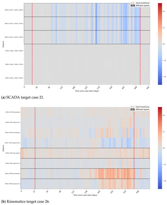
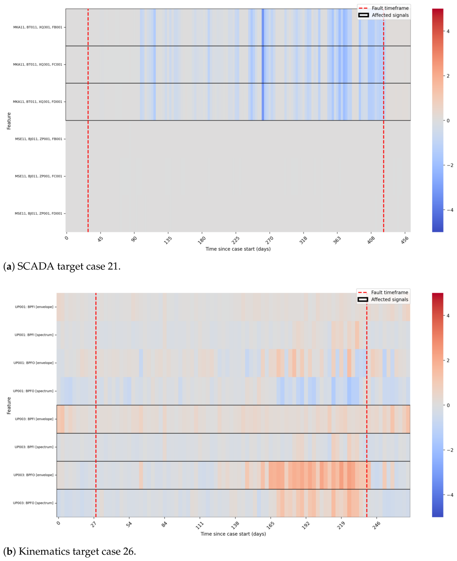
Figure 1 shows one SCADA case at the top and one kinematics case at the bottom. The marked components are the affected components, and the fault pattern is visible mainly there. The blue–white–red scale indicates negative, near-zero, and positive centered deviations.

Figure 1. Example anomaly space heatmaps for a SCADA case and a kinematics case. The marked components are affected. The fault pattern is mainly visible there. Note: The kinematics heatmap does not include full hierarchical feature names, but the hierarchical structure is still preserved. Ball pass frequency of the outer race (BPFO) is one of the bearing-frequency signals. For example, in the label UP001: BPFO, UP001 identifies a level-2 component and the part after the colon names the signal.

2.3. Diagnosis Task and Label Policy

This work addresses wind turbine component diagnosis from anomaly space embeddings. The task is case-based: for a given historical fault interval, the model predicts which turbine component is affected. The output is one component label for the target case, reduced to the first two levels of the Reference Designation System for Power Plants (RDS-PP).

RDS-PP is a hierarchical designation system for power plant objects and documentation. For wind-power plants, the relevant application guideline is VGB-S-823-32 [37]. In this dataset, RDS-PP labels describe wind turbine components and subcomponents with four comma-separated hierarchy levels. For example, the label BFA11, BT001, XQ001, FB001 can be read as a path through the component hierarchy. The first entry BFA11 gives the coarsest component group available in the label, BT001 refines this group, and the remaining entries XQ001 and FB001 describe finer subcomponent levels.

Real fault cases are rare, unevenly distributed across turbines, and documented through maintenance records. In this benchmark, a case contains one historical fault interval together with metadata for the turbine unit, affected component, and approximate start and end times. These interval annotations are coarse: the recorded interval does not necessarily match the exact onset and end of the signal pattern. Some faults, especially sensor faults, may also appear intermittently within the case interval. Therefore, the evaluation is performed at case level.

We use the first two RDS-PP levels jointly as the diagnosis label. In the example above, the evaluated label would therefore be BFA11, BT001. We refer to this two-level label as the RDS-PP level-2 diagnosis label. This aggregation is used because levels 3 and 4 encode signal-specific information, such as the measured physical quantity or an aggregation level, which is not directly relevant as a diagnosis label for component diagnosis. Non-defect samples receive the intermediate label Normal. During target case evaluation, windows outside the known target fault interval are not part of the case-level diagnosis, and the label Normal is excluded from the final component decision. The benchmark therefore assumes that a candidate fault interval is already given and evaluates which component is affected. Automatic detection, segmentation, and proposal of candidate fault intervals are outside the scope of the benchmark.

2.4. Source–Target Transfer Setting

The main learning difficulty is cross-machine transfer under domain shift. Source cases come from different turbines and operating histories, while the held-out target case has no diagnosis labels available during training, feature selection, or hyperparameter selection. Source rows from the same turbine unit as the target case are excluded to reduce leakage through unit-specific behavior.

A sample or window is the model input associated with one timestamp after the preprocessing and window construction steps described in Section 3. The vector x contains the anomaly space features of that sample or window, y denotes its source-domain training label, u denotes the turbine unit, and c denotes the case.

$${\mathcal{D}}_s={\left\{(x_i^s,y_i^s,u_i^s,c_i^s)\right\}}_{i=1}^{n_s},{\mathcal{D}}_t={\left\{(x_j^t,u^t,c^t)\right\}}_{j=1}^{n_t},u_i^s\ne u^t.$$

(1)

In Equation (1), ${\mathcal{D}}_s$ denotes $n_s$ labeled source windows and ${\mathcal{D}}_t$ denotes $n_t$ unlabeled target windows. The condition $u_i^s\ne u^t$ expresses the same-unit exclusion rule for the target unit.

For each fold, ${\mathcal{D}}_t$ comprises the preprocessed windows from the held-out case whose timestamps fall within the known fault interval. These windows are used by domain adaptation models and target-dependent HPO objectives.

Let ${\mathcal{Y}}_s$ denote the set of component labels observed in the source data, and let $y_t$ denote the hidden true component label of the target case. In the maintained benchmark, a target case is evaluated only if $y_t\in {\mathcal{Y}}_s$. Negative transfer can nevertheless occur because ${\mathcal{Y}}_s$ may contain additional component labels that are irrelevant to the target case. If adaptation aligns target windows with such source-only labels, the final diagnosis can be worse than a source-only prediction. This motivates partial adaptation methods that reduce the influence of unlikely source-only classes while still using unlabeled target data.

2.5. Anomaly Space Representation

Diagnosis starts from anomaly space embeddings. The representation is motivated by a sparse deviation assumption: during component faults, only a limited subset of related signals is expected to deviate strongly at the same time. Instead of simulating faults, the model is trained on inputs corrupted with artificial disturbances and learns to estimate those disturbances for each signal.

The embeddings are produced by a neural network called denoiser [35]. Here, denoiser does not refer to a denoising autoencoder. The model does not reconstruct clean inputs but predicts signal-wise disturbance values from synthetically corrupted inputs. Each output value corresponds to an input signal and estimates the disturbance associated with that signal. The anomaly space embeddings are therefore interpreted as anomaly scores, where large values indicate signals for which the model estimates a strong disturbance relative to learned normal behavior. The anomaly space is used as input data for the diagnosis models evaluated in this paper.

Training is performed by adding synthetic disturbances to input vectors and learning to recover the injected disturbance vector. For sample b and input feature j, let $x_{b,j}$ denote the undisturbed input, ${ϵ}_{b,j}$ the injected synthetic disturbance, and

$${\tilde{x}}_{b,j}=x_{b,j}+{ϵ}_{b,j}$$

(2)

the corrupted input. The denoiser $g_{\theta }$ receives the corrupted vector, optionally together with context information such as turbine and time embeddings and predicts a disturbance vector:

$${\widehat{ϵ}}_b=g_{\theta }\left({\tilde{x}}_b\right).$$

(3)

The training objective is minimizing the mean absolute error between injected and predicted disturbances using the following loss function:

$$L_{\mathrm{dist}}={\displaystyle \frac{1}{B}}{\displaystyle \sum _{b=1}^B}{\displaystyle \sum _{j=1}^d}\left|{\widehat{ϵ}}_{b,j}-{ϵ}_{b,j}\right|.$$

(4)

Equation (3) defines the denoiser prediction for the corresponding disturbance vector. In Equation (4), B is the batch size, and d is the number of input features. The index b denotes samples or windows, while j denotes features. The loss trains the denoiser to recover the injected disturbance vector.

The synthetic disturbances are sampled from a sparse distribution:

$${ϵ}_{b,j}\sim \sqrt{1+2\gamma }\mathcal{N}(0,1)·\mathrm{Beta}({\gamma }^{-1},1).$$

(5)

Equation (5) uses the standard normal distribution $\mathcal{N}(0,1)$ and a beta-distributed scaling factor $\mathrm{Beta}({\gamma }^{-1},1)$. The parameter $\gamma$ controls how many signals are perturbed on average: smaller values create broader perturbations, whereas larger values concentrate the disturbance on fewer signals. The prefactor $\sqrt{1+2\gamma }$ sets the disturbance variance to one for all values of $\gamma$. For the embeddings used in this study, $\gamma$ is increased from 1 to 16 during training and the batch size is $2^{14}$. The denoiser was trained unsupervised on all available data, including observations from cases later used for validation and testing. The representation-learning stage is therefore transductive with respect to the benchmark case pool. Neither component labels nor fault interval start and end times were used during this stage. The model was primarily influenced by the predominance of normal data, which reduced the need to filter the training data to healthy samples only.

The denoiser is inspired by ARCANA [38]. Both approaches seek signal-level disturbances that explain anomalous behavior. In contrast to ARCANA, which derives corrections through a post-hoc optimization step around reconstruction errors of an autoencoder, the denoiser directly predicts the disturbance vector. This paper uses the resulting anomaly space embeddings to benchmark cross-machine component diagnosis models.

3. Materials and Methods

3.1. Diagnosis Inputs and Label Construction

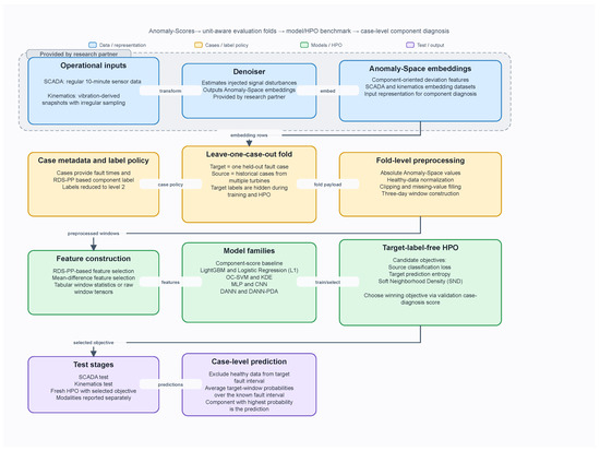
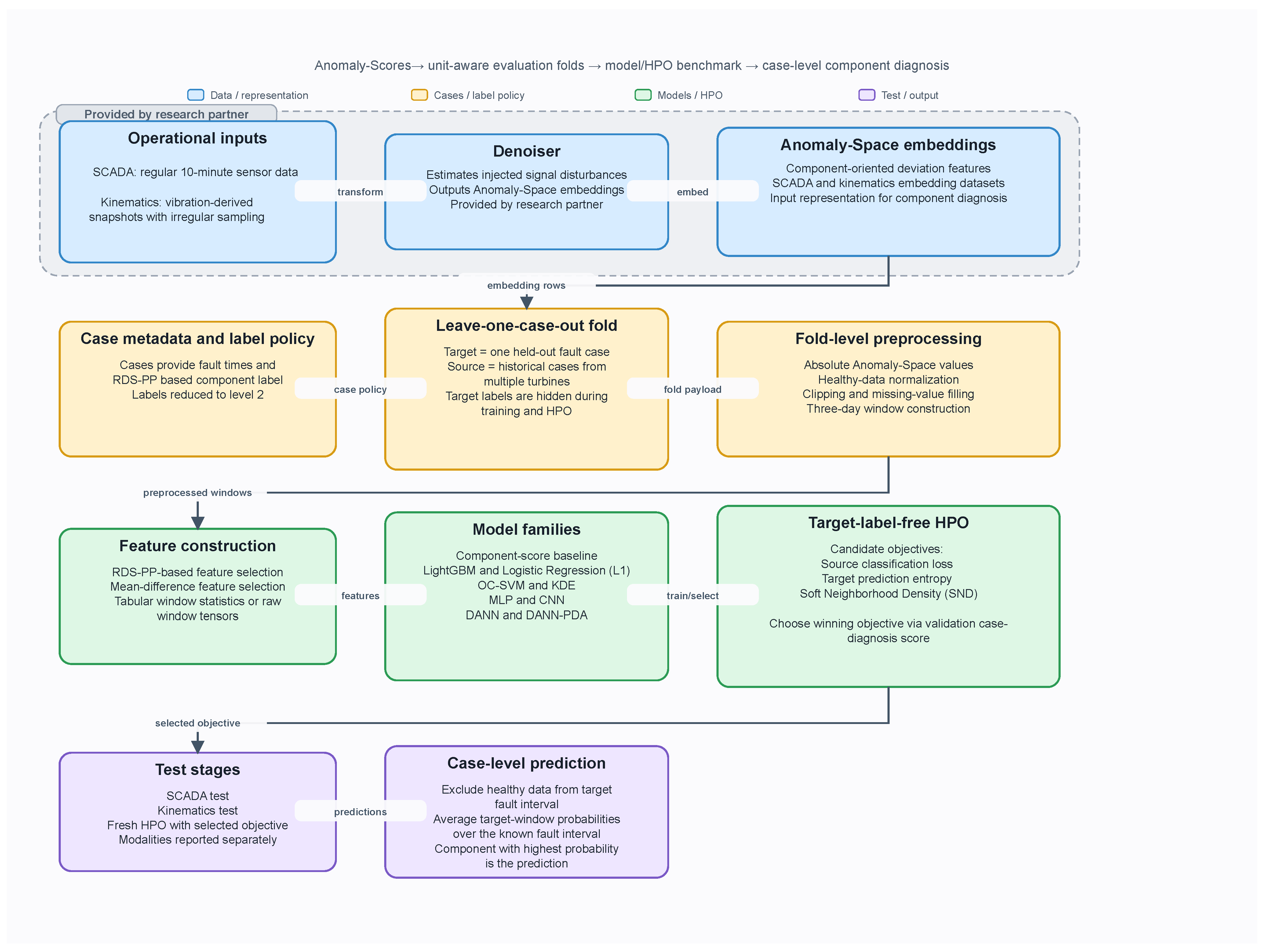
Each observation belongs to a turbine unit and to one historical fault case. SCADA and kinematics are treated as separate diagnosis datasets with separate sets of cases, but they follow the same high-level evaluation logic. In the available benchmark, the SCADA case pool consists of documented sensor-related fault cases, including loose contacts, whereas the kinematics case pool consists of documented bearing-fault cases derived from vibration data. The input features are anomaly space embeddings produced by the neural denoiser described in Section 2. Metadata columns identify the case, turbine unit, fault interval, and raw RDS-PP target component, while the power class provides operating context. The overall benchmark workflow from anomaly space embeddings to case-level component diagnosis is summarized in Figure 2. Summary statistics for the available benchmark data are reported in Table 1. The SCADA and kinematics case-pool compositions by component label are shown in Table 2 and Table 3.

Figure 2. Overview of the benchmark workflow for case-based wind turbine component diagnosis from anomaly space embeddings.

Table 1. Dataset statistics for the anomaly score-based embedding benchmark.

Statistic	Value	Comment
SCADA benchmark cases	29	Documented sensor-related fault cases: 23 HPO objective selection cases and 6 test cases
SCADA turbine units	16	Distinct turbine units represented by the SCADA benchmark cases
SCADA RDS-PP level-2 labels	8	Component labels at the diagnosis granularity
SCADA samples	726,827	Samples across all SCADA benchmark cases
SCADA fault interval samples	567,183	Samples inside annotated SCADA fault intervals
SCADA features	334	After metadata removal
Kinematics test cases	7	Documented bearing-fault cases used as kinematics target cases
Kinematics turbine units	5	Distinct turbine units represented by the kinematics test cases
Kinematics RDS-PP level-2 labels	3	Component labels at the diagnosis granularity
Kinematics samples	8155	Samples across kinematics test cases
Kinematics fault interval samples	6654	Samples inside annotated kinematics fault intervals
Kinematics features	227	After metadata removal

Table 2. SCADA HPO objective selection and test cases.

Component	Case IDs	Turbine Units	Samples	Fault Interval Samples
MDK20, BT013	107, 226, 242 *, 264, 279, 405, 522, 740	6	108,565	60,866
MDK20, BT701	166 *, 245, 263, 599	4	38,236	19,419
MDX10, None	51, 355, 1056 *, 1073	4	222,412	199,534
MKA11, BT111	21, 413	2	60,149	49,472
MST11, BT011	275 *, 417, 749	3	89,715	75,781
MST11, BT012	148 *, 149, 533	3	103,181	86,865
MST11, BT013	246, 274, 334 *	3	53,319	35,409
MST11, BT021	619, 1019	2	51,250	39,837

* denotes a SCADA test case. All other listed SCADA cases belong to the HPO objective selection pool.

Table 3. Kinematics test cases.

RDS-PP Level-2 Label	Case IDs	Turbine Units	Samples	Fault Interval Samples
MDK10, UP001	418, 698	2	2505	2006
MDK20, UP901	105, 176	2	3414	3052
MKA11, UP003	26, 832, 911	3	2236	1596

All listed kinematics cases are test cases.

The benchmark uses case-level maintenance annotations for supervision. Samples inside the annotated defect interval inherit the case component label, reduced to the first two RDS-PP levels. Samples outside the annotated defect interval receive the intermediate label Normal. This construction provides source labels for supervised training, but it does not imply that every window inside a fault interval contains the fault pattern. The target case is treated as unlabeled with respect to its component label during training and HPO. The target interval itself is known because the benchmark evaluates diagnosis of an existing candidate case.

$$y_i=\left\{\begin{array}{cc}\mathrm{Normal},\hfill & \mathrm{if}\mathrm{sample}i\mathrm{is}\mathrm{outside}\mathrm{the}\mathrm{annotated}\mathrm{fault}\mathrm{interval},\hfill \\ y_{\mathrm{RDS}2},\hfill & \mathrm{if}\mathrm{sample}i\mathrm{is}\mathrm{inside}\mathrm{the}\mathrm{annotated}\mathrm{fault}\mathrm{interval}.\hfill \end{array}\right.$$

(6)

In Equation (6), $y_{\mathrm{RDS}2}$ is the level-2 RDS-PP diagnosis label of the corresponding case.

3.2. Preprocessing

Preprocessing is applied separately inside each case to avoid data leakage. The benchmark uses absolute anomaly space values. Healthy period centering then subtracts a healthy interval mean from each feature. For source and target cases, this mean is estimated from pre-fault data.

A normalized and upper-clipped feature is written as

$${\tilde{x}}_{ij}=min\left\{\left||x_{ij}|-{\mu }_{j,\mathrm{healthy}}\right|,x_{max}\right\}.$$

(7)

In Equation (7), $x_{ij}$ is anomaly space feature j at sample i, ${\mu }_{j,\mathrm{healthy}}$ is the healthy interval mean used for centering, and $x_{max}$ is the upper clipping limit. The implementation uses $x_{max}=5$. Missing feature values are filled in time order separately within each fault and non-fault interval. Feature columns are then aligned between source and target data so that only shared features are passed to the models.

3.3. Windowed-Time Representation

Anomaly space embeddings are converted into non-overlapping three-day windows before model training and evaluation. Window construction is performed separately for each case and each contiguous pre-fault or fault interval. Post-fault observations are removed during preprocessing. Each source window inherits the label of the interval from which it is constructed.

During window construction, observations are up-sampled to a regular 10 min grid. Multiple observations within the same grid interval are averaged, and empty grid positions are filled by forward-fill and backward-fill. Classical machine learning models, one-class models, and multi-layer perceptron (MLP) models use the mean, maximum, and standard deviation of these windows, whereas convolutional neural network (CNN) models use the resulting fixed-length window tensors.

Table 4 summarizes shared input construction settings and Table 5 the extracted window features.

Table 4. Shared preprocessing and input construction settings used across model families.

Workflow Step	Setting
Windowing policy	Three-day windows
Feature reduction	Included in the grid search configuration for non-baseline models: RDS-PP-based selection followed by group-wise principal component analysis (PCA), or mean difference selection. The component score baseline only uses RDS-PP-based feature selection
Preprocessing	Absolute value transformation of anomaly score-based embeddings, healthy period centering, feature clipping and missing value filling

Table 5. Model-specific input representations after windowing.

Models	Model Input
Classical, one-class, and MLP models	Mean, maximum, and standard deviation over each three-day window
CNN models	Raw three-day window tensors without summary statistic extraction

3.4. Feature Selection and Reduction

Two feature reduction configurations are included in the grid search for all non-baseline models. For each configuration, feature selection and principal component analysis (PCA) fitting are performed separately within each fold using source data only. The resulting feature subset and fitted transformations are then applied unchanged to the held-out target data.

RDS-PP-based feature selection keeps signals whose RDS-PP prefix matches the source component labels at the first two hierarchy levels. In the rdspp_then_group_pca configuration, this selection is followed by group-wise PCA. SCADA signals are grouped by their first two RDS-PP levels, whereas kinematics signals are grouped by the UPxxx prefix preceding the colon. For each group containing at least two signals, a PCA model is fitted to the source data and the group is replaced by its first principal component.

Mean difference feature selection ranks the signals separately for each source case by the absolute difference between their fault period and healthy period means. The union of the five highest-ranked signals from each source case forms the selected feature set.

$$s_{c,j}=\left|{\displaystyle \frac{1}{|{\mathcal{I}}_{c,\mathrm{fault}}^s|}}\sum _{i\in {\mathcal{I}}_{c,\mathrm{fault}}^s}{\tilde{x}}_{ij}-{\displaystyle \frac{1}{|{\mathcal{I}}_{c,\mathrm{healthy}}^s|}}\sum _{i\in {\mathcal{I}}_{c,\mathrm{healthy}}^s}{\tilde{x}}_{ij}\right|.$$

(8)

The score $s_{c,j}$ ranks feature j for source case c by the absolute difference between its fault period and healthy period means. The sets ${\mathcal{I}}_{c,\mathrm{fault}}^s$ and ${\mathcal{I}}_{c,\mathrm{healthy}}^s$ contain the corresponding source case indices.

3.5. Model Families

The benchmark compares component-oriented classical baselines, supervised source-only models, one-class density models, neural source-only models, and adversarial domain adaptation models. The compared model families are summarized in Table 6. Implementation details for the individual models are listed in Table 7.

Table 6. Model families considered in the anomaly space benchmark.

Model Family	Models	Role in the Benchmark
Baseline	Component score baseline	Component-oriented reference that aggregates anomaly score evidence over the target fault interval
Classical supervised models	LightGBM, Logistic Regression ($L_1$)	Source-supervised tabular models for anomaly space window statistics
One-class and density baselines	OC-SVM, KDE	Source distribution models that can filter normal-looking windows inside coarse fault interval annotations
Neural supervised models	MLP, CNN	Nonlinear source-only classifiers for tabular features and raw window tensors
Adversarial adaptation	DANN-MLP, DANN-CNN	Adversarial source–target alignment using unlabeled target windows
Partial adaptation	DANN-PDA-MLP, DANN-PDA-CNN	Adversarial alignment with target prediction-based class weighting under partial label space mismatch

Table 7. Implementation details of the evaluated model variants.

Model	Input	Estimator or Architecture	Training or Scoring Rule
Component score baseline	Target fault interval features	No fitted estimator. Selected anomaly space features are mapped to RDS-PP component labels	Highest target-interval feature mean
LightGBM	Tabular window statistics	Multiclass gradient-boosted decision trees	Source-supervised multiclass prediction
Logistic Regression ($L_1$)	Tabular window statistics	Min-max-scaled, class-balanced logistic regression with $L_1$ penalty and saga solver	Source-supervised cross-entropy. The $L_1$ penalty can zero feature coefficients
OC-SVM	Tabular window statistics	One radial basis function (RBF) OC-SVM per source label, including Normal	Class-wise decision function scores, normalized over labels, normal-like filtering
KDE	Tabular window statistics	One Gaussian kernel density estimator per source label, including Normal	Class-wise log likelihoods, normalized over labels, normal-like filtering
MLP	Tabular window statistics	One MLP feature layer with initial width 8 and a classifier head with 5 hidden units, ReLU, a linear output layer, and softmax probabilities	Source-supervised cross-entropy with Adam optimizer
CNN	Raw window tensors	One-dimensional convolution with 32 filters and kernel width 16, ReLU, max pooling, adaptive average pooling, and classifier head with 5 hidden units, ReLU, linear output layer, and softmax probabilities	Source-supervised cross-entropy with Adam optimizer
DANN-MLP	Tabular window statistics plus unlabeled target windows	MLP feature extractor, source classifier with 5 hidden units, ReLU, linear output layer, and softmax probabilities, and linear binary domain discriminator	Source cross-entropy plus adversarial domain loss through gradient reversal
DANN-CNN	Raw window tensors plus unlabeled target windows	CNN feature extractor, source classifier with 5 hidden units, ReLU, linear output layer, and softmax probabilities, and linear binary domain discriminator	Source cross-entropy plus adversarial domain loss through gradient reversal
DANN-PDA-MLP	Tabular window statistics plus unlabeled target windows	DANN-MLP with target prediction-based source-class weights	Weighted source and adversarial losses, AUS regularization
DANN-PDA-CNN	Raw window tensors plus unlabeled target windows	DANN-CNN with target prediction-based source-class weights	Weighted source and adversarial losses, AUS regularization

• Component score baseline

The component score baseline directly uses the anomaly space embedding semantics. Let $W_c$ be the windows in the target fault interval of case c, let $\rho \left(j\right)$ map feature j to its RDS-PP level-2 component label, and let ${\mathcal{J}}_c$ be the set of features whose mapped component is an eligible non-Normal source label. The baseline averages each eligible feature over the target interval and predicts the component associated with the largest mean:

$${\overline{x}}_{c,j}={\displaystyle \frac{1}{|W_c|}}\sum _{w\in W_c}{\tilde{x}}_{w,j},{\widehat{y}}_c=\rho \left(\underset{j\in {\mathcal{J}}_c}{arg\; max}{\overline{x}}_{c,j}\right).$$

(9)

In Equation (9), ${\overline{x}}_{c,j}$ is the target-interval mean of feature j, and ${\widehat{y}}_c$ is the resulting case-level prediction. The baseline has no learned parameters and no hyperparameter search. It is included because anomaly space features are already component-oriented. Therefore, a simple aggregation rule is an interpretable and intuitive reference.

• Supervised source-only models

Light Gradient Boosting Machine (LightGBM) is used as a supervised gradient boosting model on tabular window features. $L_1$-regularized logistic regression is included as a supervised model that can reduce the effective feature set through its $L_1$ penalty. The MLP is a nonlinear source-only classifier on tabular window features, and the CNN is a source-only classifier on raw window tensors. These models use labeled source windows only during supervised training.

• One-class and density models

One-class support vector machine (OC-SVM) and kernel density estimation (KDE) are used as density-based baselines without explicit discriminative multi-class training. For each method, a Normal model is fitted to the source windows labeled Normal. The Boolean filter_normal_like grid parameter determines whether this model is used to filter component-labeled source fault interval windows before fitting the component-specific models. When filtering is enabled, OC-SVM retains these windows if the Normal model classifies them as outliers. KDE retains them if their log likelihood under the Normal model is below the mean minus three standard deviations of the log likelihoods of the Normal source windows. When filtering is disabled, all source windows with the corresponding component label are used. A separate class-specific model is then fitted for each component.

At inference time, each target window receives one compatibility score per source label, including Normal: OC-SVM uses class-specific decision function scores, and KDE uses class-specific log likelihoods. The scores are normalized over labels to obtain probability-like vectors.

• Domain adaptation models

The Domain-Adversarial Neural Network (DANN) [17] is an adversarial domain adaptation model that uses labeled source windows and unlabeled target windows. It consists of a feature extractor, a source label classifier, and a binary domain discriminator. The feature extractor should remain discriminative for source labels while making source and target features difficult to distinguish by the discriminator.

The source classification loss is

$$L_{\mathrm{cls}}=-{\displaystyle \frac{1}{n_s}}{\displaystyle \sum _{i=1}^{n_s}}log{p}_{\theta }\left(y_i^s\mid x_i^s\right).$$

(10)

In Equation (10), $L_{\mathrm{cls}}$ is the mean source-domain negative log-likelihood over the $n_s$ labeled source samples. The DANN objective combines source classification with adversarial domain alignment. Let $q_{{\theta }_d}(d\mid f_{{\theta }_f}\left(x\right))$ be the domain discriminator probability for domain label d after feature extraction, where $d=0$ denotes source and $d=1$ denotes target. The domain discrimination loss is

$$L_{\mathrm{dom}}=-{\displaystyle \frac{1}{n_s+n_t}}\left[{\displaystyle \sum _{i=1}^{n_s}}log{q}_{{\theta }_d}(0\mid f_{{\theta }_f}\left(x_i^s\right))+{\displaystyle \sum _{j=1}^{n_t}}log{q}_{{\theta }_d}(1\mid f_{{\theta }_f}\left(x_j^t\right))\right].$$

(11)

The DANN objective is then

$$\underset{{\theta }_f,{\theta }_y}{min}\underset{{\theta }_d}{max}\left[L_{\mathrm{cls}}({\theta }_f,{\theta }_y)-{\lambda }_{\mathrm{adv}}{L}_{\mathrm{dom}}({\theta }_f,{\theta }_d)\right].$$

(12)

In Equation (12), ${\theta }_f$, ${\theta }_y$, and ${\theta }_d$ are the parameters of the feature extractor, source label classifier, and domain discriminator, respectively. The term $L_{\mathrm{dom}}$ is the binary domain discrimination loss from Equation (11), and ${\lambda }_{\mathrm{adv}}$ controls the strength of adversarial alignment. At training iteration r, the gradient reversal layer multiplies the backward feature gradient by $-g_r$, where $g_r=2/(1+exp(-10r/R))-1$ and R is the total number of training iterations. The fixed coefficient 10 controls how quickly the reversal strength approaches 1. Thus, the discriminator minimizes $L_{\mathrm{dom}}$, while the feature extractor receives a reversed domain gradient and learns features that are less domain-specific.

DANN with partial-domain adaptation (DANN-PDA) is a partial-domain adaptation variant motivated by Balanced Adversarial Alignment and Adaptive Uncertainty Suppression (BA³US) [27]. It is used when the target label space is expected to be a subset of the source label space. Standard adversarial alignment can be harmful in this setting, because target samples may be aligned with source-only classes. The model therefore estimates class-level source weights from predictions on the unlabeled target case. These weights are used in source classification and adversarial alignment, so source classes that appear relevant for the target case have more influence and unlikely source-only classes have less influence.

Balanced Adversarial Alignment (BAA) denotes the corresponding weighted adversarial alignment term. It keeps the DANN idea of making source and target features difficult to distinguish, but biases the alignment toward source classes that are likely to be present in the target case. In the BA³US formulation, this is achieved by adding weighted source examples to the target side of the domain alignment loss, which stabilizes early alignment and reduces the influence of source-only classes. Adaptive Uncertainty Suppression (AUS) addresses uncertainty propagation from source predictions. Instead of considering only the probability of the correct source class, AUS also checks how much probability remains on the wrong classes. Source predictions that still assign high probability to wrong classes are penalized, so uncertain source representations have less influence during adaptation.

The objective of this implementation combines weighted source classification, AUS, and balanced adversarial alignment through the same gradient reversal mechanism:

$$\underset{{\theta }_f,{\theta }_y}{min}\underset{{\theta }_d}{max}{L}_{\mathrm{cls}}^w({\theta }_f,{\theta }_y)+{\beta }_{\mathrm{AUS}}{L}_{\mathrm{wce}}^w({\theta }_f,{\theta }_y)+{\lambda }_{\mathrm{adv}}{L}_{\mathrm{adv}}^{\mathrm{ba}}({\theta }_f,{\theta }_d).$$

(13)

In Equation (13), ${\theta }_f$, ${\theta }_y$, and ${\theta }_d$ are the parameters of the feature extractor, source label classifier, and domain discriminator. The term $L_{\mathrm{cls}}^w$ is the weighted source classification loss, $L_{\mathrm{wce}}^w$ is the confidence-weighted complement entropy form of AUS, and $L_{\mathrm{adv}}^{\mathrm{ba}}$ is the BAA domain alignment term. The parameters ${\beta }_{\mathrm{AUS}}$ and ${\lambda }_{\mathrm{adv}}$ control the strength of AUS and adversarial alignment. The internal AUS exponent $\xi$ and the BAA balance parameter $\mu$ are fixed to 1 in all runs.

3.6. Target Label-Free Hyperparameter Selection

In the target case setting, the component label of the held-out case is not available when model hyperparameters are selected. Hyperparameter selection must therefore rely on metrics that can be computed from labeled source data and unlabeled target data only. We apply different target label-free HPO objectives: source classification loss, target prediction entropy, and Soft Neighborhood Density (SND) [39]. Source classification loss tests whether the model still fits labeled source cases. For each fitted grid search configuration, the source classification loss in Equation (10) is evaluated on the same labeled source windows used to fit that configuration.

Target entropy rewards confident predictions on the unlabeled target case, but it can select overconfident wrong models under label space mismatch. SND evaluates the local structure in the target prediction space by converting pairwise target-sample similarities into soft-neighborhood distributions. Higher SND scores indicate denser target neighborhoods without using target labels. Grid search is used to select the model configuration for each source–target fold and the target label-free HPO objective chooses the configuration with the lowest objective value.

After target label-free grid selection is completed for all validation folds, validation target labels are revealed only to compare the candidate HPO objectives. After configuration selection, the validation case diagnosis score is computed for each model and HPO objective. The scores are then averaged across models, and the objective with the highest average validation score is selected for the test stages. Exact ties are resolved in the fixed order of source classification loss, target entropy, and SND. Test labels are not used during HPO or model training.

A single HPO objective is used for all HPO-tuned models to keep the model selection criterion fixed across the benchmark and to limit model-specific adaptation to the relatively small validation pool. Selecting a separate objective for each model would introduce additional validation label-informed decisions and increase the risk of overfitting the validation cases. The selected objective should therefore be interpreted as the most effective shared selection criterion on average, rather than as the optimal objective for every individual model. The component score baseline is excluded from this selection because it does not use HPO.

Target entropy is computed as

$$J_{\mathrm{ent}}={\displaystyle \frac{1}{n_t}}{\displaystyle \sum _{i=1}^{n_t}}\left[-{\displaystyle \sum _{k=1}^K}{p}_{\theta }(k\mid x_i^t)log{p}_{\theta }(k\mid x_i^t)\right].$$

(14)

In Equation (14), $n_t$ is the number of unlabeled target samples, K is the number of output classes, and $p_{\theta }(k\mid x_i^t)$ is the model probability assigned to class k for target sample $x_i^t$. Minimizing this objective favors confident target predictions, but it does not verify whether those confident predictions are correct.

The SND score is computed from soft neighborhoods as

$$\begin{array}{cc}\hfill {\overline{z}}_i^t& ={\displaystyle \frac{z_i^t}{{\parallel z_i^t\parallel }_2}},s_{ij}=⟨{\overline{z}}_i^t,{\overline{z}}_j^t⟩,\hfill \\ \hfill {\alpha }_{ij}& ={\displaystyle \frac{exp(s_{ij}/\tau )}{{\sum }_{\begin{array}{c}\ell =1\\ \ell \ne i\end{array}}^{n_t}exp(s_{i\ell }/\tau )}},j\ne i,\hfill \\ \hfill H_{\mathrm{SND}}& =-{\displaystyle \frac{1}{n_t}}{\displaystyle \sum _{i=1}^{n_t}}{\displaystyle \sum _{\begin{array}{c}j=1\\ j\ne i\end{array}}^{n_t}}{\alpha }_{ij}log{\alpha }_{ij},J_{\mathrm{SND}}=-H_{\mathrm{SND}}.\hfill \end{array}$$

(15)

In Equation (15), $z_i^t$ and $z_j^t$ are target softmax output vectors before similarity normalization. The normalized vector ${\overline{z}}_i^t$ is obtained by L2-normalizing $z_i^t$, and $s_{ij}$ is the inner product between two normalized target vectors. Self-similarities are excluded by restricting the neighborhood index to $j\ne i$. The coefficient ${\alpha }_{ij}$ is the soft-neighborhood weight assigned by sample i to sample j after temperature scaling. Since we define HPO as a minimization problem, the implemented objective is $J_{\mathrm{SND}}=-H_{\mathrm{SND}}$. The temperature is fixed at $\tau =0.05$ for all models and grid search configurations.

3.7. Evaluation and Case-Level Aggregation

The final diagnosis is made at case level rather than at individual-window level. This is necessary because many SCADA cases are sensor faults caused by effects such as loose contacts. Such faults can appear intermittently: within an annotated fault interval, some windows show the fault pattern, whereas other windows can look normal. Since the complete interval inherits the component label, a model that correctly predicts Normal for normal-looking windows inside the interval would nevertheless be penalized in a window-level evaluation. Window-level correctness can therefore be overly pessimistic for the operational diagnosis task.

For a target case c, the set $W_c$ contains all target windows whose timestamps fall inside the known fault interval. Target windows outside this interval are not used for final case-level component evaluation. The model produces a class probability vector, or normalized class compatibility vector for one-class models, for each window $w\in W_c$. These vectors are averaged across the fault interval to obtain one aggregated component score:

$${\overline{p}}_c\left(k\right)={\displaystyle \frac{1}{|W_c|}}\sum _{w\in W_c}{p}_{\theta }(k\mid x_w),{\widehat{y}}_c=\underset{k\in \mathcal{Y}\setminus \left\{\mathrm{Normal}\right\}}{arg\; max}{\overline{p}}_c\left(k\right).$$

(16)

In Equation (16), ${\overline{p}}_c\left(k\right)$ is the aggregated score assigned to class k for target case c. The label Normal is excluded from the final argmax because the target interval is known to correspond to a fault case.

The primary evaluation metric is the case diagnosis score. It measures the fraction of evaluated target cases for which the predicted component matches the target component label. For case c and evaluation run r, the binary case diagnosis score $d_{c,r}$ is defined as 1 for a correct diagnosis and 0 for an incorrect diagnosis:

$$d_{c,r}=\left\{\begin{array}{cc}1,\hfill & \mathrm{if}{\widehat{y}}_{c,r}=y_c,\hfill \\ 0,\hfill & \mathrm{otherwise},\hfill \end{array}\right.{\overline{d}}_c={\displaystyle \frac{1}{R_c}}{\displaystyle \sum _{r=1}^{R_c}}{d}_{c,r},S_{\mathrm{diag}}={\displaystyle \frac{1}{\left|\mathcal{C}\right|}}\sum _{c\in \mathcal{C}}{\overline{d}}_c.$$

(17)

In Equation (17), ${\widehat{y}}_{c,r}$ is the predicted component in run r, $y_c$ is the true target component label of case c, $R_c$ is the number of evaluation runs for that case, and $\mathcal{C}$ is the set of evaluated target cases. The reported score $S_{\mathrm{diag}}$ is therefore the mean of the per-case scores ${\overline{d}}_c$ over all evaluated cases. For models evaluated once, $R_c=1$. For each neural network-based model, the final test evaluation was repeated five times using different random seeds, so $R_c=5$. The values $d_{c,r}$ were averaged across the five runs. Thus, a value such as $0.40$ indicates that two of five repeated test runs predicted the correct component. Aggregate case diagnosis accuracy is calculated for every final repeat and then summarized across repeats. Classical and one-class models have one deterministic final fit.

3.8. Repeat Variability and Case Stability

Neural models were evaluated over five repeated final refits with different random seeds. For each model and dataset, we report the mean, sample standard deviation, and range of the repeat-level case diagnosis score. At case level, ${\overline{d}}_c$ denotes the fraction of repeated runs that diagnosed case c correctly. Cases with $0<{\overline{d}}_c<1$ are considered outcome-unstable because their correctness changes across runs. The number of distinct predicted components and the modal-prediction rate additionally characterize prediction instability.

4. Experimental Setup

4.1. Overall Protocol

The experiments follow a unit-aware leave-one-case-out protocol. In every fold, one case is held out as the unlabeled target case. All eligible cases from other turbine units form the labeled source pool. Source rows from the same turbine unit as the target case are excluded before preprocessing, feature selection, model training, and HPO.

The experimental design has three stages. First, the SCADA HPO objective selection stage compares target label-free HPO objectives on validation cases. Second, the SCADA test stage evaluates all models, with the selected HPO objective fixed for all HPO-tuned models. Third, the kinematics test stage evaluates the models on vibration-derived kinematics embeddings, again using the selected HPO objective for all HPO-tuned models.

Because the number of available kinematics cases is too small to support a separate HPO objective selection stage, the kinematics stage is test-only. The same HPO objective selected in the SCADA stage is used for all kinematics cases.

4.2. Target Label-Free Grid Search

Hyperparameter selection is implemented as deterministic grid search over small predefined search spaces. For each model, each candidate configuration contains model hyperparameters and, for all non-baseline models, the feature reduction configuration.

The candidate target label-free objectives are source classification loss (Equation (10)), target entropy (Equation (14)), and SND (Equation (15)). All objectives are stored as minimization objectives. For SND, the negative SND value is minimized. The component score baseline has fixed settings and therefore does not use grid search.

Table 8 summarizes the model-specific grid search spaces.

Table 8. Grid search spaces used for target label-free model selection.

Model	Grid Evaluation	Model-Specific Grid Choices
Component score baseline	No HPO search	Fixed feature reduction baseline_rdspp_based_fs with feature-to-component mapping over target-interval means
LightGBM	Full grid per fold with one training run per grid point	max_depth $\{3,6\}$; estimators $\left\{100\right\}$; feature fraction $\left\{0.7\right\}$; minimum data per leaf $\{5,20\}$; $L_1$ regularization $\{0,0.5\}$
Logistic Regression ($L_1$)	Full grid per fold with one training run per grid point	Inverse regularization strength $C\in \{0.01,0.1,1.0\}$; maximum iterations $\left\{5000\right\}$; tolerance $\left\{0.001\right\}$; min-max feature scaling; $L_1$ penalty, saga solver, and balanced class weights
OC-SVM	Full grid per fold with one training run per grid point	RBF kernel; $\nu \in \{0.02,0.05,0.1\}$; $\gamma \in \{\mathtt{scale},0.03\}$; normal-like filtering {true, false}
KDE	Full grid per fold with one training run per grid point	Gaussian kernel; bandwidth $\{0.05,0.1,0.3\}$; normal-like filtering {true, false}
MLP	Full grid per fold with one training run per grid point	Batch size $\left\{8\right\}$; 30 epochs; one MLP feature layer with initial width $\left\{8\right\}$; classifier head with 5 hidden units, ReLU, linear output layer, and softmax probabilities; Adam optimizer; learning rate $0.003$
CNN	Full grid per fold with one training run per grid point	Batch size $\left\{8\right\}$; 30 epochs; one-dimensional CNN feature extractor; classifier head with 5 hidden units, ReLU, linear output layer, and softmax probabilities; Adam optimizer; learning rate $0.003$
DANN-MLP	Full grid per fold with one training run per grid point	MLP grid; linear discriminator; discriminator learning rate $0.003$; adversarial weight ${\lambda }_{\mathrm{adv}}\in \{0.1,0.5,1.0\}$; gradient reversal schedule coefficient 10
DANN-CNN	Full grid per fold with one training run per grid point	CNN grid; linear discriminator; discriminator learning rate $0.003$; adversarial weight ${\lambda }_{\mathrm{adv}}\in \{0.1,0.5,1.0\}$; gradient reversal schedule coefficient 10
DANN-PDA-MLP	Full grid per fold with one training run per grid point	DANN-MLP grid plus ${\beta }_{\mathrm{AUS}}\in \{0,0.5\}$; $\xi =1$; $\mu =1$; class-weight update interval 2 epochs
DANN-PDA-CNN	Full grid per fold with one training run per grid point	DANN-CNN grid plus ${\beta }_{\mathrm{AUS}}\in \{0,0.5\}$; $\xi =1$; $\mu =1$; class-weight update interval 2 epochs

Unless stated otherwise, two feature reduction methods are considered during grid search for each non-baseline model: rdspp_then_group_pca and mean_based_fs. Hyperparameters not listed in the table use the corresponding package or implementation defaults. The reported model implementations used the following package versions: scikit-learn 1.7.2, PyTorch 2.8.0, and LightGBM 4.6.0. OC-SVM and KDE use the scikit-learn implementations. Neural networks were built using PyTorch. For neural and adversarial models, the final evaluation is repeated with five random seeds after the grid-selected configuration has been chosen.

4.3. SCADA HPO Objective Selection Stage

The SCADA HPO objective selection stage defines the validation folds used to choose the target label-free HPO objective. It uses 23 SCADA cases, which are listed in Table 9. Leave-one-case-out cross-validation is applied within this pool. In each fold, one case is treated as the unlabeled target case, while the remaining eligible SCADA cases serve as source cases after same-unit exclusion. The output is the selected target label-free HPO objective for subsequent test experiments.

Table 9. Case pools and evaluation stages in the anomaly space benchmark.

Stage	Case Pool	Source–Target Split	Purpose
SCADA HPO objective selection	21, 51, 107, 149, 226, 245, 246, 263, 264, 274, 279, 355, 405, 413, 417, 522, 533, 599, 619, 740, 749, 1019, 1073	Leave-one-case-out over HPO objective selection cases with same-unit source rows excluded	Choose the target label-free HPO objective
SCADA test	148, 166, 242, 275, 334, 1056	Use HPO objective selection cases as the source pool. Evaluate each test case as target with same-unit source rows excluded	Run per-case grid search with the selected objective and report case diagnosis scores
Kinematics test	26, 105, 176, 418, 698, 832, 911	Leave-one-case-out over test cases with same-unit source rows excluded	Run per-case grid search with the SCADA-selected objective and report case diagnosis scores

Note: Target component labels are hidden during preprocessing, feature selection, grid search, and model training in all stages. They are revealed only for validation objective comparison in the SCADA HPO objective selection stage and for final evaluation in the test stages.

4.4. SCADA Test Stage

The SCADA test stage estimates diagnosis performance for models whose hyperparameters are selected with the chosen target label-free HPO objective. It uses six test target cases, which are listed in Table 9. For each target case, all eligible SCADA cases from the HPO objective selection pool are used as source data, with rows from the same turbine unit as the target case excluded. Target labels remain hidden during preprocessing, feature selection, HPO, and model training. They are used only for the final case-level evaluation reported in Section 5.

4.5. Kinematics Test Stage

The kinematics test stage evaluates the same selected HPO objective on kinematics anomaly space embeddings. It uses 7 kinematics cases, which are also listed in Table 9.

5. Results

This section reports the SCADA HPO objective selection results, the SCADA test results, and the kinematics test results.

5.1. SCADA HPO Objective Selection Results

Table 10 summarizes the validation-stage comparison of the three target label-free HPO objectives. Source classification loss achieves the highest mean validation case diagnosis score, followed by target entropy and SND. The subsequent SCADA and kinematics test stages therefore use source classification loss as the HPO objective.

Table 10. SCADA HPO objective selection results averaged over models. Target labels are used only after grid search configuration selection to compute the validation case diagnosis score.

HPO Objective	Validation Case Diagnosis Score
Source classification loss	$\mathbf{0.243}\pm \mathbf{0.025}$
Target entropy	$0.217\pm 0.039$
SND	$0.213\pm 0.031$

Values are the mean ± standard error across the ten searchable models. All objectives select from the same deterministic grids.

The difference is a shared-objective result rather than evidence that source classification loss is best for every model. Table 11 shows the substantial model-specific variation underlying the average.

Table 11. Model-specific SCADA validation case diagnosis scores for the target label-free HPO objectives. Bold values mark the highest score for each model, including equal scores.

Model	Source Classification Loss	Target Entropy	SND
LightGBM	$0.217$	$\mathbf{0.348}$	$0.304$
Logistic Regression ($L_1$)	$0.391$	$\mathbf{0.435}$	$0.130$
OC-SVM	$0.130$	$\mathbf{0.174}$	$\mathbf{0.174}$
KDE	$\mathbf{0.261}$	$0.130$	$0.087$
MLP	$0.261$	$0.261$	$\mathbf{0.348}$
CNN	$0.217$	$\mathbf{0.348}$	$\mathbf{0.348}$
DANN-MLP	$0.130$	$0.174$	$\mathbf{0.217}$
DANN-CNN	$\mathbf{0.217}$	$0.130$	$0.130$
DANN-PDA-MLP	$\mathbf{0.304}$	$0.087$	$0.130$
DANN-PDA-CNN	$\mathbf{0.304}$	$0.087$	$0.261$
Mean ± standard error across models	$\mathbf{0.243}\pm \mathbf{0.025}$	$0.217\pm 0.039$	$0.213\pm 0.031$

Table 12 reports the exploratory comparison of the candidate objectives.

Table 12. Exploratory sensitivity of test accuracy to the HPO objective. Values average the ten searchable models.

HPO Objective	SCADA Accuracy	Kinematics Accuracy
Source classification loss	$\mathbf{0.383}$	$\mathbf{0.314}$
Target entropy	$0.317$	$0.257$
SND	$0.333$	$0.271$

Taken together, the validation results identify source classification loss as the best shared criterion on average, not as a universally superior criterion. Target entropy can reward confident predictions for a wrong source-only class, and SND can favor a compact target cluster assigned to an incorrect component.

Importantly, source classification loss ranks first only under the predefined rule that averages the case diagnosis scores across models. Under a voting-based comparison, with equal scores resolved by the same fixed objective order, source classification loss and target entropy each receive four votes, while SND receives two. Thus, no objective obtains a majority. If equal scores are instead counted as joint wins, all three objectives are best for four models. This alternative view shows that these results should not be interpreted as a statistically significant difference between the HPO objectives.

5.2. SCADA Test Results

Table 13 reports the SCADA test case diagnosis scores using source classification loss as the selected target label-free HPO objective. The component score baseline achieves the strongest result on the six SCADA test cases with an accuracy of $0.833$. Among learned models, KDE is highest (accuracy $0.500$), followed by DANN-CNN and DANN-PDA-MLP (both $0.433$). Neural and domain-adaptive models do not consistently improve over the simpler methods.

Table 13. SCADA test case diagnosis scores using source classification loss as the selected target label-free HPO objective.

Model	148	166	242	275	334	1056	Accuracy
Component score baseline	$1.00$	$1.00$	$1.00$	$1.00$	$0.00$	$1.00$	$\mathbf{0.833}$
LightGBM	$0.00$	$0.00$	$1.00$	$0.00$	$0.00$	$1.00$	$0.333$
Logistic Regression ($L_1$)	$0.00$	$0.00$	$1.00$	$0.00$	$0.00$	$1.00$	$0.333$
OC-SVM	$0.00$	$0.00$	$0.00$	$0.00$	$0.00$	$1.00$	$0.167$
KDE	$0.00$	$0.00$	$1.00$	$1.00$	$0.00$	$1.00$	$0.500$
MLP	$0.00$	$0.00$	$1.00$	$0.40$	$0.00$	$1.00$	$0.400\pm 0.091$
CNN	$0.00$	$0.20$	$1.00$	$0.20$	$0.00$	$0.80$	$0.367\pm 0.183$
DANN-MLP	$0.00$	$0.00$	$0.80$	$0.20$	$0.00$	$0.80$	$0.300\pm 0.139$
DANN-CNN	$0.20$	$0.40$	$0.80$	$0.40$	$0.00$	$0.80$	$0.433\pm 0.190$
DANN-PDA-MLP	$0.00$	$0.00$	$1.00$	$0.60$	$0.00$	$1.00$	$0.433\pm 0.091$
DANN-PDA-CNN	$0.00$	$0.00$	$1.00$	$0.40$	$0.00$	$1.00$	$0.400\pm 0.091$

Case entries are diagnosis success rates. Neural entries and accuracy average five final refits. Their accuracy column gives the repeat mean ± sample standard deviation. Deterministic models have one final fit, so no repeat SD is shown.

5.3. Kinematics Test Results

Table 14 reports the kinematics test results using source classification loss as the SCADA-selected HPO objective. OC-SVM obtains the highest accuracy ($0.714$), whereas DANN-PDA-CNN is the strongest neural model by accuracy ($0.286$). The ranking differs from SCADA, consistent with the distinct, sparsely sampled vibration-derived representation and the smaller source pool.

Table 14. Kinematics test case diagnosis scores using source classification loss as the SCADA-selected target label-free HPO objective.

Model	26	105	176	418	698	832	911	Accuracy
Component score baseline	$0.00$	$0.00$	$0.00$	$1.00$	$1.00$	$1.00$	$0.00$	$0.429$
LightGBM	$0.00$	$1.00$	$1.00$	$0.00$	$0.00$	$0.00$	$0.00$	$0.286$
Logistic Regression ($L_1$)	$0.00$	$1.00$	$1.00$	$0.00$	$0.00$	$0.00$	$0.00$	$0.286$
OC-SVM	$1.00$	$1.00$	$1.00$	$0.00$	$0.00$	$1.00$	$1.00$	$\mathbf{0.714}$
KDE	$0.00$	$1.00$	$1.00$	$0.00$	$0.00$	$0.00$	$0.00$	$0.286$
MLP	$0.00$	$0.40$	$1.00$	$0.00$	$0.00$	$0.00$	$0.00$	$0.200\pm 0.078$
CNN	$0.60$	$0.00$	$1.00$	$0.00$	$0.00$	$0.00$	$0.00$	$0.229\pm 0.078$
DANN-MLP	$0.00$	$0.60$	$1.00$	$0.00$	$0.00$	$0.00$	$0.00$	$0.229\pm 0.078$
DANN-CNN	$0.00$	$0.20$	$1.00$	$0.00$	$0.00$	$0.00$	$0.00$	$0.171\pm 0.064$
DANN-PDA-MLP	$0.00$	$0.80$	$1.00$	$0.00$	$0.00$	$0.00$	$0.00$	$0.257\pm 0.064$
DANN-PDA-CNN	$0.00$	$1.00$	$1.00$	$0.00$	$0.00$	$0.00$	$0.00$	$0.286\pm 0.000$

Case entries are diagnosis success rates. Neural entries and accuracy average five final refits. Their accuracy column gives the repeat mean ± sample standard deviation. Deterministic models have one final fit, so no repeat SD is shown.

5.4. Variability Across Repeated Neural Runs

Table 15 summarizes variability in the aggregate case diagnosis score across repeated neural refits. The standard deviation and range describe sensitivity to initialization on the fixed test cases.

Table 15. Case diagnosis performance across repeated neural refits. Values in the mean ± standard deviation columns are calculated across repeat-level aggregate case diagnosis scores.

Model	SCADA Mean ± SD	SCADA Range	Kinematics Mean ± SD	Kinematics Range
MLP	$0.400\pm 0.091$	$0.333$–$0.500$	$0.200\pm 0.078$	$0.143$–$0.286$
CNN	$0.367\pm 0.183$	$0.167$–$0.667$	$0.229\pm 0.078$	$0.143$–$0.286$
DANN-MLP	$0.300\pm 0.139$	$0.167$–$0.500$	$0.229\pm 0.078$	$0.143$–$0.286$
DANN-CNN	$0.433\pm 0.190$	$0.167$–$0.667$	$0.171\pm 0.064$	$0.143$–$0.286$
DANN-PDA-MLP	$0.433\pm 0.091$	$0.333$–$0.500$	$0.257\pm 0.064$	$0.143$–$0.286$
DANN-PDA-CNN	$0.400\pm 0.091$	$0.333$–$0.500$	$0.286\pm 0.000$	$0.286$–$0.286$

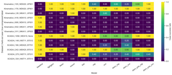
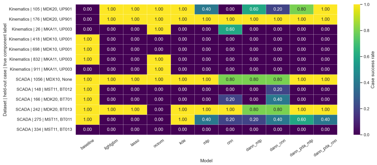
Figure 3 shows whether repeat variability is distributed across many cases or concentrated in a small number of difficult target cases. Intermediate success rates identify cases whose correctness changes across repeated runs.

Figure 3. Per-case diagnosis success rates. Neural cells report the fraction of five final refits that predicted the correct component, while deterministic-model cells report their single outcome. SCADA and kinematics are displayed separately. Row labels identify the dataset, held-out case, and true component label.

Table 16 identifies the cases responsible for outcome or prediction instability. Outcome instability means that correctness changes across runs ($0<{\overline{d}}_c<1$). Prediction-only instability means that multiple wrong components are predicted while correctness remains unchanged.

Table 16. Target cases with outcome or prediction instability across five neural final refits.

Dataset	Case (True Component)	Outcome-Unstable Models	Additional Prediction-Only Unstable Models
SCADA	148 (MST11, BT012)	DANN-CNN	DANN-MLP
SCADA	166 (MDK20, BT701)	CNN, DANN-CNN	–
SCADA	242 (MDK20, BT013)	DANN-MLP, DANN-CNN	–
SCADA	275 (MST11, BT011)	All six neural models	–
SCADA	334 (MST11, BT013)	–	MLP, CNN, DANN-CNN, both DANN-PDA models
SCADA	1056 (MDX10, None)	CNN, DANN-MLP, DANN-CNN	–
Kinematics	26 (MKA11, UP003)	CNN	DANN-MLP
Kinematics	105 (MDK20, UP901)	MLP, DANN-MLP, DANN-CNN, DANN-PDA-MLP	–
Kinematics	698 (MDK10, UP001)	–	DANN-CNN
Kinematics	911 (MKA11, UP003)	–	DANN-MLP, DANN-CNN

On SCADA, DANN-CNN is the most initialization-sensitive model: five of six cases are outcome-unstable and every case receives more than one predicted component across the five refits. Its repeat-level accuracy spans $0.167$–$0.667$. Case 275 is unstable for every neural model, whereas case 334 is always misdiagnosed but receives changing wrong labels from five neural models. On kinematics, outcome instability is concentrated in cases 26 and 105. DANN-PDA-CNN is repeat-stable but remains correct on only two of seven cases.

5.5. Computational Requirements

Measurements were obtained on an Apple M5 Pro system with 15 CPU cores and 24 GiB RAM, running macOS 26.5.2 and Python 3.12.13. PyTorch models used the CPU. The available Apple Metal backend was not used. HPO time is the elapsed interval from the first trial start to the last completion for one final target fold. Final fit and inference values are reported as the mean ± sample standard deviation across official final fits. Peak worker process resident set size (RSS) is the corresponding mean and was sampled every 100 ms.

Table 17 summarizes the corresponding computational requirements for the SCADA final stage.

Table 17. Representative computational requirements for the SCADA final stage. HPO values summarize the six target folds. Final fit, inference, and RSS values summarize official final repeats.

Model	HPO per Fold (min)	Final Fit (s)	Inference (ms)	Peak RSS (GiB)
Component score baseline	–	<0.01	$0.11\pm 0.01$	$0.82$
LightGBM	$0.54\pm 0.01$	$3.94\pm 0.14$	$1.65\pm 0.21$	$0.90$
Logistic Regression ($L_1$)	$0.45\pm 0.02$	$25.32\pm 3.50$	$1.19\pm 0.02$	$0.91$
OC-SVM	$0.01\pm 0.01$	$0.01\pm 0.00$	$3.17\pm 0.91$	$0.90$
KDE	$0.03\pm 0.01$	<0.01	$15.23\pm 9.82$	$0.91$
MLP	$0.03\pm 0.00$	$2.49\pm 0.21$	$0.53\pm 0.27$	$0.40$
CNN	$1.98\pm 0.03$	$14.28\pm 2.63$	$3.00\pm 1.58$	$1.27$
DANN-MLP	$0.08\pm 0.00$	$4.12\pm 0.34$	$0.57\pm 0.30$	$0.40$
DANN-CNN	$4.71\pm 0.12$	$25.74\pm 3.79$	$3.65\pm 2.45$	$1.20$
DANN-PDA-MLP	$0.27\pm 0.00$	$7.79\pm 0.59$	$0.56\pm 0.29$	$0.41$
DANN-PDA-CNN	$8.49\pm 0.16$	$29.44\pm 6.17$	$3.03\pm 2.10$	$1.22$

CNN-based adversarial models are the most expensive. DANN-PDA-CNN requires about 8.5 min of HPO per SCADA fold and 29.4 s per final fit, whereas MLP HPO and fitting require about 0.03 min and 2.5 s, respectively. Kinematics is smaller: the largest mean final fit time is 5.10 s for DANN-PDA-CNN. Inference remains below 16 ms on average for every model and dataset.

5.6. Cross-Model and Cross-Dataset Patterns

Across the SCADA and kinematics datasets, simple baselines remain competitive with more complex neural and domain-adaptive models. The DANN and DANN-PDA variants do not show a consistent advantage in the current test tables, despite being designed to use unlabeled target-domain data. This suggests that, in the current benchmark, realistic case-based labels, small target case pools, and partial label spaces make reliable improvements difficult to obtain.

The locked source classification loss trials select mean_based_fs in 54 of 60 searchable SCADA final folds and 69 of 70 kinematics final folds. rdspp_then_group_pca is selected in the remaining six and one folds, respectively. Both reductions therefore remain in every model’s grid, but the mean-based reduction dominates the selected final configurations.

The results also indicate that SCADA and kinematics should be treated as distinct diagnostic views. SCADA benefits from regular sampling and contains many sensor and thermal variables, whereas kinematics is more directly connected to drivetrain mechanics but is sparse and operating state dependent. The strongest method for one dataset is therefore not necessarily the strongest method for the other.

6. Discussion

The results support the usefulness of anomaly space embeddings as compact, component-oriented inputs for cross-machine wind turbine component diagnosis. At the same time, the comparison shows that the component diagnosis remains difficult even when the input representation is designed to emphasize deviations from learned normal behavior. The component score baseline performs best on SCADA, whereas OC-SVM achieves the highest kinematics accuracy (Table 13 and Table 14). OC-SVM correctly diagnoses all MKA11 and MDK20 cases but misclassifies both MDK10 cases. Its weaker SCADA result may be related to the larger number of component classes and greater overlap between their patterns. Given the small number of test cases, this result does not show guarantee that OC-SVM is generally better suited to kinematics data. In the current benchmark, model complexity did not overcome the difficulty of coarse fault interval annotations, rare cases, and source–target distribution shifts.

Conceptually, this study integrates anomaly score-based representations, partial domain adaptation, target label-free HPO, and case-based cross-machine evaluation in one framework. The test pools contain only six SCADA and seven kinematics cases. The case results show no consistent gain from adversarial alignment on this benchmark.

A central interpretation is that the anomaly space representation already performs part of the normalization that domain adaptation models are intended to learn. If the embedding space suppresses much of the turbine-specific operating behavior, adversarial alignment has less remaining domain discrepancy to exploit. Conversely, if relevant differences remain, the small number of cases and partial label space mismatch make adversarial alignment unstable. Aligning target samples with the wrong source classes can be more harmful than leaving the source-trained classifier unchanged, especially when the target case contains only one component label.

The target label-free HPO results are important for deployment. Since the target component label is unavailable during model selection, the selected configuration must be chosen using source labels and unlabeled target data only. In the SCADA HPO objective selection stage, source classification loss has the highest across-model average among the tested objectives (Table 10). Thus, retaining source-domain discriminability is the selected shared signal for the available validation cases, although model-specific rankings vary. Target entropy can select overconfident but wrong models under partial label space mismatch, while SND can favor compact target predictions without guaranteeing that the compact cluster corresponds to the true component. Because no separate kinematics validation pool was available, the kinematics results remain conditional on transferring the SCADA-selected HPO objective and do not establish which objective an independent kinematics validation pool would select.

Label uncertainty is another limitation. The fault intervals come from operational maintenance records and provide practical supervision, but they are not exact pointwise ground truth. In particular, sensor faults can appear intermittently inside an annotated case interval, and normal-looking windows inside a fault interval may still receive the fault component label. The case-level aggregation used in this paper is therefore appropriate for the operational question of which component to inspect, but it cannot fully resolve uncertainty around the exact onset, duration, or intermittency of the underlying fault pattern.

The preprocessing uses target pre-fault data for healthy period centering. This relies on the assumption that the candidate fault interval is already known. Therefore, the reported task should be interpreted as component diagnosis for already defined candidate cases.

The same-unit exclusion rule is important for data leakage control. Without excluding source cases from the target turbine, turbine-specific behavior could inflate performance. The resulting problem is deliberately strict: the model must transfer from historical cases on other turbines to an unlabeled target case on a held-out turbine. This setup reflects the intended deployment scenario more closely than random window-level splits, but it also reduces the amount of eligible source data for some target cases.

The comparison between the SCADA and kinematics datasets underlines their complementary diagnostic views. SCADA provides regular low-frequency operating and temperature information and is useful for sensor faults and slower thermal effects. Kinematics provides vibration-derived frequency-domain information that is relevant for drivetrain and bearing faults, but its sampling is sparse and depends on suitable operating states. The present study evaluates both datasets separately. Future work should investigate principled SCADA-kinematics fusion, but such fusion must preserve the same leakage constraints: no target component labels during HPO, no same-unit source data, and no use of case information that would not be available in the intended deployment setting.

Several limitations should be considered when interpreting the results. First, the test pools contain only six SCADA and seven kinematics cases, representing five turbines in each dataset. Formal model comparisons are not reliable with so few independent cases. We therefore did not perform formal significance testing and instead report repeat variability and case-level stability directly. Five neural final refits show initialization sensitivity, most strongly for SCADA DANN-CNN and case 275. The reported scores should therefore be treated as case-study evidence. Second, the denoiser was trained on observations from the complete benchmark case pool, including cases later used for validation and testing. The representation-learning stage is therefore transductive and does not evaluate a denoiser trained only on cases that are completely disjoint from the evaluation cases. The denoiser is not updated during diagnosis model training, and the diagnosis models cannot fine-tune the representation jointly with the diagnosis objective. Third, the benchmark evaluates diagnosis of already defined candidate intervals, not automatic detection of new fault intervals. Fourth, the HPO budget is intentionally limited for computational feasibility, which may disadvantage higher-capacity neural and adversarial models. Fifth, the study does not include a controlled ablation of DANN-PDA. The HPO grid allows AUS to be disabled by setting ${\beta }_{\mathrm{AUS}}=0$, and the DANN variants provide a reference without the PDA extensions. However, these comparisons do not isolate the individual effects of BAA, AUS, and class weighting. Sixth, the three-day window length was fixed a priori as an engineering compromise between temporal context for intermittent or coarsely annotated faults and retaining enough non-overlapping windows. No window length sensitivity experiment was conducted. Finally, raw industrial wind turbine data cannot be released due to confidentiality restrictions. The transformed anomaly score-based embeddings, however, are available through a request process.

7. Conclusions

This paper studies cross-machine wind turbine component diagnosis from SCADA and vibration-derived kinematics anomaly score embeddings. The benchmark combines case-based leave-one-out validation, RDS-PP level-2 labels, target label-free HPO, and case-level aggregation. The framework is designed to reflect a realistic deployment setting in which a candidate fault interval is available, but the affected component is unknown.

The experiments compare a component score baseline, supervised classical models, one-class density models, neural source-only models, and adversarial domain adaptation variants. The component score baseline obtains the highest SCADA accuracy ($0.833$), while OC-SVM obtains the highest kinematics accuracy ($0.714$). Adversarial domain adaptation does not consistently improve case-level diagnosis performance. The small number of independent cases does not support reliable formal model comparisons. Five neural refits reveal that instability is model- and case-specific, with SCADA DANN-CNN and case 275 showing the strongest sensitivity.

The main conclusion is that credible cross-machine wind turbine component diagnosis requires more than applying increasingly complex transfer learning models. Case-based evaluation, explicit label policies, target label-free model selection, and strong component-oriented baselines are important for obtaining interpretable performance estimates. The results also indicate that real-world component diagnosis remains challenging because verified fault cases are rare, fault interval annotations are coarse, source and target cases and turbines can differ substantially, and partial label space mismatch can cause negative transfer.

Future work should expand the number of evaluated fault cases, investigate fusion of SCADA and kinematics embeddings, and study hierarchical RDS-PP diagnosis in which coarse component groups and finer component labels are evaluated jointly. Methods that explicitly handle few-shot component classes, uncertain case intervals, and partial label spaces are particularly promising directions for improvement.

References

- Fraunhofer Institute for Solar Energy Systems ISE. German Public Electricity Generation in 2025: Wind and Solar Power Take the Lead; Fraunhofer Institute for Solar Energy Systems ISE: Freiburg, Germany, 2026; Available online: https://www.ise.fraunhofer.de/en/press-media/press-releases/2026/german-public-electricity-generation-in-2025-wind-and-solar-power-take-the-lead.html (accessed on 17 January 2026).
- Martini, M.; Guanche, R.; Losada-Campa, I.; Losada, I. The impact of downtime over the long-term energy yield of a floating wind farm. Renew. Energy 2018, 117, 1–11. [Google Scholar] [CrossRef] [Scilit]
- Tian, Z.; Zhang, H. Wind farm predictive maintenance considering component level repairs and economic dependency. Renew. Energy 2022, 192, 495–506. [Google Scholar] [CrossRef] [Scilit]
- Udo, W.; Muhammad, Y. Data-Driven Predictive Maintenance of Wind Turbine Based on SCADA Data. IEEE Access 2021, 9, 162370–162388. [Google Scholar] [CrossRef] [Scilit]
- Han, T.; Xie, W.; Pei, Z. Semi-supervised adversarial discriminative learning approach for intelligent fault diagnosis of wind turbine. Inf. Sci. 2023, 648, 119496. [Google Scholar] [CrossRef] [Scilit]
- Badihi, H.; Zhang, Y.; Jiang, B.; Pillay, P.; Rakheja, S. A Comprehensive Review on Signal-Based and Model-Based Condition Monitoring of Wind Turbines: Fault Diagnosis and Lifetime Prognosis. Proc. IEEE 2022, 110, 754–806. [Google Scholar] [CrossRef] [Scilit]
- Alagha, N.; Khairuddin, A.S.M.; Haitaamar, Z.N.; Al-Khatib, O.; Kanesan, J. Artificial Intelligence in Wind Turbine Fault Detection and Diagnosis: Advances and Perspectives. Energies 2025, 18, 1680. [Google Scholar] [CrossRef] [Scilit]
- Zheng, H.; Wang, R.; Yang, Y.; Yin, J.; Li, Y.; Li, Y.; Xu, M. Cross-Domain Fault Diagnosis Using Knowledge Transfer Strategy: A Review. IEEE Access 2019, 7, 129260–129290. [Google Scholar] [CrossRef] [Scilit]
- Liu, J.; Qu, F.; Hong, X.; Zhang, H. A Small-Sample Wind Turbine Fault Detection Method With Synthetic Fault Data Using Generative Adversarial Nets. IEEE Trans. Ind. Inform. 2019, 15, 3877–3888. [Google Scholar] [CrossRef] [Scilit]
- Zhang, G.; Li, Y.; Jiang, W.; Shu, L. A fault diagnosis method for wind turbines with limited labeled data based on balanced joint adaptive network. Neurocomputing 2022, 481, 133–153. [Google Scholar] [CrossRef] [Scilit]
- Zhao, Z.; Jiao, Y.; Xu, Y.; Chen, Z.; Zio, E. A fault diagnosis framework using unlabeled data based on automatic clustering with meta-learning. Eng. Appl. Artif. Intell. 2025, 139, 109584. [Google Scholar] [CrossRef] [Scilit]
- Zhao, Z.; Zhang, Q.; Yu, X.; Sun, C.; Wang, S.; Yan, R.; Chen, X. Applications of Unsupervised Deep Transfer Learning to Intelligent Fault Diagnosis: A Survey and Comparative Study. IEEE Trans. Instrum. Meas. 2021, 70, 3525828. [Google Scholar] [CrossRef] [Scilit]
- Shao, S.; McAleer, S.; Yan, R.; Baldi, P. Highly Accurate Machine Fault Diagnosis Using Deep Transfer Learning. IEEE Trans. Ind. Inform. 2019, 15, 2446–2455. [Google Scholar] [CrossRef] [Scilit]
- Xing, Z.; Liu, Y.; Wang, Q.; Fu, J. Fault diagnosis of rotating parts integrating transfer learning and ConvNeXt model. Sci. Rep. 2025, 15, 190. [Google Scholar] [CrossRef] [Scilit] [PubMed]
- Li, Y.; Jiang, W.; Zhang, G.; Shu, L. Wind turbine fault diagnosis based on transfer learning and convolutional autoencoder with small-scale data. Renew. Energy 2021, 171, 103–115. [Google Scholar] [CrossRef] [Scilit]
- Wilson, G.; Cook, D.J. A Survey of Unsupervised Deep Domain Adaptation. ACM Trans. Intell. Syst. Technol. 2020, 11, 1–46. [Google Scholar] [CrossRef] [Scilit] [PubMed]
- Ganin, Y.; Ustinova, E.; Ajakan, H.; Germain, P.; Larochelle, H.; Laviolette, F.; March, M.; Lempitsky, V. Domain-Adversarial Training of Neural Networks. J. Mach. Learn. Res. 2016, 17, 1–35. [Google Scholar]
- Chen, P.; Zhao, R.; He, T.; Wei, K.; Yang, Q. Unsupervised domain adaptation of bearing fault diagnosis based on Join Sliced Wasserstein Distance. ISA Trans. 2022, 129, 504–519. [Google Scholar] [CrossRef] [Scilit] [PubMed]
- An, Y.; Zhang, K.; Chai, Y.; Liu, Q.; Huang, X. Domain adaptation network base on contrastive learning for bearings fault diagnosis under variable working conditions. Expert Syst. Appl. 2023, 212, 118802. [Google Scholar] [CrossRef] [Scilit]
- Liang, P.; Wang, B.; Jiang, G.; Li, N.; Zhang, L. Unsupervised fault diagnosis of wind turbine bearing via a deep residual deformable convolution network based on subdomain adaptation under time-varying speeds. Eng. Appl. Artif. Intell. 2023, 118, 105656. [Google Scholar] [CrossRef] [Scilit]
- Zhong, J.; Lin, C.; Gao, Y.; Zhong, J.; Zhong, S. Fault diagnosis of rolling bearings under variable conditions based on unsupervised domain adaptation method. Mech. Syst. Signal Process. 2024, 215, 111430. [Google Scholar] [CrossRef] [Scilit]
- Liu, J.; Wan, L.; Xie, F.; Sun, Y.; Wang, X.; Li, D.; Wu, S. Cross-machine deep subdomain adaptation network for wind turbines fault diagnosis. Mech. Syst. Signal Process. 2024, 210, 111151. [Google Scholar] [CrossRef] [Scilit]
- Zhang, Z.; Chen, H.; Li, S.; An, Z. Unsupervised domain adaptation via enhanced transfer joint matching for bearing fault diagnosis. Measurement 2020, 165, 108071. [Google Scholar] [CrossRef] [Scilit]
- Liao, Y.; Huang, R.; Li, J.; Chen, Z.; Li, W. Dynamic Distribution Adaptation Based Transfer Network for Cross Domain Bearing Fault Diagnosis. Chin. J. Mech. Eng. 2021, 34, 52. [Google Scholar] [CrossRef] [Scilit]
- Zhu, Y.; Pei, Y.; Wang, A.; Xie, B.; Qian, Z. A partial domain adaptation scheme based on weighted adversarial nets with improved CBAM for fault diagnosis of wind turbine gearbox. Eng. Appl. Artif. Intell. 2023, 125, 106674. [Google Scholar] [CrossRef] [Scilit]
- Xu, X.; Yang, X.; He, C.; Shi, P.; Hua, C. Adversarial Domain Adaptation Model Based on LDTW for Extreme Partial Transfer Fault Diagnosis of Rotating Machines. IEEE Trans. Instrum. Meas. 2024, 73, 3538811. [Google Scholar] [CrossRef] [Scilit]
- Liang, J.; Wang, Y.; Hu, D.; He, R.; Feng, J. A Balanced and Uncertainty-Aware Approach for Partial Domain Adaptation. In Proceedings of the Computer Vision—ECCV, Virtually, 23–28 August 2020; Vedaldi, A., Bischof, H., Brox, T., Frahm, J.M., Eds.; Springer: Cham, Switzerland, 2020; pp. 123–140. [Google Scholar] [CrossRef] [Scilit]
- Liu, S.; Jiang, H.; Wu, Z.; Yi, Z.; Wang, R. Intelligent fault diagnosis of rotating machinery using a multi-source domain adaptation network with adversarial discrepancy matching. Reliab. Eng. Syst. Saf. 2023, 231, 109036. [Google Scholar] [CrossRef] [Scilit]
- Yang, S.; Kong, X.; Wang, Q.; Li, Z.; Cheng, H.; Yu, L. A multi-source ensemble domain adaptation method for rotary machine fault diagnosis. Measurement 2021, 186, 110213. [Google Scholar] [CrossRef] [Scilit]
- Zhang, G.; Kong, X.; Wang, Q.; Du, J.; Xu, K.; Wang, J.; Ma, H. Multi-source partial domain adaptation method based on pseudo-balanced target domain for fault diagnosis. Knowl.-Based Syst. 2024, 284, 111255. [Google Scholar] [CrossRef] [Scilit]
- Wang, M.; Chen, Y.; Xiao, L. Multisource partial domain adaptation for bearing fault diagnosis. J. Phys. Conf. Ser. 2024, 2853, 012067. [Google Scholar] [CrossRef] [Scilit]
- Yu, Y.; Guo, L.; Tan, Y.; Gao, H.; Zhang, J. Multisource Partial Transfer Network for Machinery Fault Diagnostics. IEEE Trans. Ind. Electron. 2022, 69, 10585–10594. [Google Scholar] [CrossRef] [Scilit]
- Garg, A.; Zhang, W.; Samaran, J.; Savitha, R.; Foo, C.S. An Evaluation of Anomaly Detection and Diagnosis in Multivariate Time Series. IEEE Trans. Neural Netw. Learn. Syst. 2022, 33, 2508–2517. [Google Scholar] [CrossRef] [Scilit] [PubMed]
- Holly, S.; Heel, R.; Katic, D.; Schoeffl, L.; Stiftinger, A.; Holzner, P.; Kaufmann, T.; Haslhofer, B.; Schall, D.; Heitzinger, C.; et al. Autoencoder Based Anomaly Detection and Explained Fault Localization in Industrial Cooling Systems. In Proceedings of the PHM Society European Conference, Turin, Italy, 29 June 2022; Volume 7, pp. 200–210. [Google Scholar] [CrossRef] [Scilit]
- Schlechtingen, M.; Hoinka, T.; Menzel, F.; Feigl, J.; Wissmann, S. AutoDiagCM—Automatisierte Diagnose von Schäden an Windenergieanlagen zur Reduzierung des Überwachungsaufwandes und Steigerung der Überwachungsgüte; EnBW-Teilprojekt; Technical Report; Hannover Technische Informationsbibliothek: Hannover, Germany, 2026. [Google Scholar] [CrossRef] [PubMed]
- Weber, K.; Preisach, C. Supervised Transfer Learning Framework for Fault Diagnosis in Wind Turbines. In Proceedings of the Upper-Rhine Artificial Intelligence Symposium 2024, Offenburg, Germany, 13–14 November 2024; pp. 95–104. [Google Scholar] [CrossRef]
- VGB PowerTech e.V. (vision generation benefit). RDS-PP Application Guideline Part 32: Wind Power Plants; VGB-S-823-32-2014-03-EN-DE; vgbe energy e.V.: Essen, Germany, 2014. [Google Scholar]
- Roelofs, C.M.; Lutz, M.A.; Faulstich, S.; Vogt, S. Autoencoder-based anomaly root cause analysis for wind turbines. Energy AI 2021, 4, 100065. [Google Scholar] [CrossRef] [Scilit]
- Saito, K.; Kim, D.; Teterwak, P.; Sclaroff, S.; Darrell, T.; Saenko, K. Tune it the Right Way: Unsupervised Validation of Domain Adaptation via Soft Neighborhood Density. In Proceedings of the 2021 IEEE/CVF International Conference on Computer Vision (ICCV), Virtually, 11–17 October 2021; pp. 9164–9173. [Google Scholar] [CrossRef] [Scilit]
Disclaimer/Publisher’s Note: The statements, opinions and data contained in all publications are solely those of the individual author(s) and contributor(s) and not of MDPI and/or the editor(s). MDPI and/or the editor(s) disclaim responsibility for any injury to people or property resulting from any ideas, methods, instructions or products referred to in the content. |
© 2026 by the authors. Licensee MDPI, Basel, Switzerland. This article is an open access article distributed under the terms and conditions of the Creative Commons Attribution (CC BY) license.