


Abstract
Medicinal plants grown under water stress are not simply surviving it—many respond to a mild, well-timed drought by producing more of the secondary metabolites that make them valuable, provided the stress never tips into outright damage. Growers call the useful kind eustress and the harmful kind distress, and keeping a crop inside that narrow window is a harder control problem than ordinary irrigation scheduling, especially once a cloud-connected system has to add network latency and tolerate dropped links into the mix. This paper proposes an edge artificial intelligence (AI) and Internet of Things (IoT) framework that pairs a MobileNetV2–LSTM–Transformer fusion design with a Proximal Policy Optimization (PPO) irrigation agent, keeping the whole decision loop local to the field. The fusion network itself is not trained here; what we test is the control policy alone, in a reproducible simulation of the eustress decision problem. No accuracy metric for the fusion network, no energy measurement and no secondary-metabolite outcome is reported; the stress band and distress threshold are generic modeling choices, and every control result is a property of the simulator. Five independently trained PPO agents were compared against four baselines—no irrigation, a constant dose, a threshold rule, and a carefully tuned PID controller—on 30 shared held-out weather scenarios using paired statistical tests with Holm–Bonferroni correction. The learned policy did not beat the threshold and constant-dose rules on band occupancy (13.7% versus 14.3–15.6%), and the tuned PID controller clearly outperformed it there (32.8%, p < 10−4). PPO reached the lowest distress exposure, only reaching distress 7.4% of the time, compared with 12.4–74.2% for the baselines (p < 10−4), but this is a trade-off of the tested configuration (λ3 = 6), obtained at higher water use (406 L versus 0–259 L) and lower band occupancy than the tuned PID; it is not a general advantage over PID. Pushed into an unseen heatwave, both PPO and PID held onto partial control (61.0% and 72.8% distress) while the remaining baselines essentially collapsed (about 99% distress). A reward-component ablation and a weight sweep trace this behavior back to the distress penalty specifically, with a smaller penalty weight trading some of that distress protection for higher band occupancy. No single controller came out ahead on every measure we tracked.
1. Introduction
Water is usually the tightest constraint on farming in arid and semi-arid regions, and the pressure on it is not easing. Southern Tunisia illustrates the problem well—two of the authors of the present study work there, in a region where rain is scarce and unpredictable and where irrigated agriculture leans heavily on groundwater. For most staple crops, the relationship between water and yield is fairly blunt—cut the water and you cut the harvest—so deficit-irrigation strategies are really about minimizing the loss per liter saved.
Medicinal and aromatic plants break that pattern. A number of species actually respond to mild, controlled drought by producing more of the alkaloids, terpenoids, and phenolic compounds that make them valuable in the first place [1]. Neem (Azadirachta indica) and Camphor (Cinnamomum camphora) are well-known examples grown under deliberately water-limited conditions. For a grower of these crops, withholding water is not simply about cutting costs—done carefully, it can raise the value of what comes out of the field, provided the plant is never pushed past the point of real tissue damage. Stress physiology gives us two useful words here: eustress, stress that triggers a beneficial response, and distress, stress that causes harm [2]. Plant scientists apply the same split to abiotic stress [3], and the literature on secondary metabolism is fairly consistent that what matters is both the intensity of the stress and how long it is sustained [4].
That distinction creates a control problem that conventional irrigation scheduling was never designed to solve. A standard scheduler only has to keep soil moisture above some floor. A eustress scheduler has a narrower job: keep the plant inside a band, stressed enough to switch on the metabolic response but not so stressed that it tips into damage—and that line can be crossed in a matter of hours on a hot, dry afternoon. The usual plant-based alternatives, leaf water potential or stomatal conductance measured by hand, are informative, but they are slow and they give a technician’s reading at one moment, not the continuous signal a timely decision actually needs, a gap that broader smart-irrigation-management reviews under climate-stressed conditions have also flagged [5].
Cheap IoT sensing has made continuous monitoring realistic [6], and a growing number of smart-irrigation platforms now pair soil probes and weather stations with a machine-learning scheduler [7]. In most of these systems, the sensor data travels to a remote server, and the field waits for an answer back. That design has three weaknesses once you take it out of the lab and into a remote field: every round trip adds latency, the data connection is a recurring cost, and if the link goes down, so does the controller. And a dropped connection tends to hurt most on exactly the kind of hot afternoon when a eustress episode can tip into distress within hours.
Edge computing offers a way around this by moving the computation onto a device in or near the field [8], and reports from actual farm deployments suggest it holds up in practice. With inference running at the edge, the irrigation loop keeps working even when the network does not. The control decision itself is a good fit for reinforcement learning (RL): rather than following a fixed, hand-tuned threshold, an RL agent learns a dosing policy directly from its interaction with the plant–soil system [9]. This has already been tried for a winter-wheat/corn rotation [10], tomato [11], maize [12], and almond trees [13], and reinforcement-learning-based digital twins have been surveyed more broadly across agriculture [14].
Two gaps in that body of work motivate this paper. The first is about the objective being optimized. The RL irrigation studies cited above reward water savings, yield, or profit—none of them ask the agent to hold the plant inside a stress band, which is the actual goal of a medicinal-plant grower. We also could not find a framework that proposes fusing canopy imagery with soil and weather time series into one stress estimate, sized for both perception and control to run on the same edge device—though, as we state plainly below, we stop at proposing and costing that design, and do not progress to training, validating or deploying it in this paper.
The second gap is about evidence rather than objective. Deep RL results are notoriously sensitive to the random seed, to hyperparameter choices, and to small implementation details—different implementations of the same algorithm have been shown to diverge so much in practice that swapping one for another is enough to reverse a published study’s conclusions [15]. Method rankings can reverse between environments, and when only a handful of runs are available, interval estimates matter more than single point scores. A learned controller evaluated against a bare threshold rule on a few episodes can easily look better than it really is. A fair test needs several independently trained agents, a classical controller tuned with comparable effort, paired comparisons run on identical weather conditions, and a correction for the number of statistical tests performed. We built the study around these requirements from the outset, rather than adding them after the fact.
Four research questions guide the present work:
- RQ1: Does a PPO policy keep the stress index inside the eustress band more often than simple baselines and a tuned PID controller?
- RQ2: Does the PPO policy reduce the time the plant spends in distress, and at what water cost?
- RQ3: Which terms of the reward are responsible for the behavior the policy learns?
- RQ4: Does any advantage of the learned policy survive a shift to harsher weather that was not seen in training?
The contributions of this paper can be summarized as follows:
- We formulate predictive eustress irrigation as a continuous-control Markov Decision Process (MDP) whose reward penalizes water use, distance from a target stress band, and time above the distress threshold, while adding a bonus for time spent inside the band (Section 3.5).
- We propose a multimodal fusion network (MobileNetV2 [16], LSTM [17], Transformer [18]) sized for edge deployment and report its layer-by-layer parameter and operation counts (Section 3.3 and Section 3.4); we emphasize that this network is architecturally coupled to the PPO agent [19] but is not trained or evaluated in this study—no inference-accuracy metric (e.g., MAE, RMSE, R2) or comparison against alternative fusion designs is reported, and the control experiments act on the simulated stress index directly rather than on this network’s output.
- We compare five independently seeded PPO agents against four baselines—including a PID controller tuned separately—on 30 shared held-out weather scenarios, using paired Wilcoxon and t tests with Holm–Bonferroni correction, effect sizes, and 95% confidence intervals (Section 4.3).
- We report per-seed results, a reward-component ablation, a five-point sweep of the distress-penalty weight, and an out-of-distribution (OOD) heatwave test (Section 4.5, Section 4.6, Section 4.7 and Section 4.8).
- We translate these findings into practical guidance for choosing a controller, discuss what an actual field deployment would require, and lay out the threats to validity (Section 5).
The remainder of the paper proceeds as follows. Section 2 reviews the related work. Section 3 describes the system architecture, the fusion network, the MDP formulation, the agent, the baseline controllers, and the experimental and statistical protocol. Section 4 reports the results, Section 5 discusses them, and Section 6 concludes.
2. Related Work
2.1. IoT Sensing and Smart Irrigation
The sensing side of precision agriculture is fairly mature by now. Soussi et al. [6] reviewed how smart sensors and the data pipelines built around them now underpin precision agriculture—from field-level sensing devices through communication links to the analytics layer that acts on the data—and later irrigation-specific surveys concluded that water-use efficiency improves the most when good sensing is paired with a closed-loop controller, since sensing alone is not enough. Mohammed et al. [20] revisited this landscape in a 2025 review spanning IoT sensing, AI-based scheduling and sustainability goals, and reached the same conclusion from a more recent vantage point: sensing infrastructure and connectivity are now mature enough that the open problem has shifted to where the decision logic runs and how it is evaluated, not whether the sensors themselves work.
Machine learning sits on top of that sensing layer, reviewed elsewhere for yield prediction, disease detection, weed detection and water management, and for the broader shift toward data-driven farm management. Qian et al. [7] surveyed smart-irrigation systems from a cyber–physical systems perspective, cataloguing how sensing, prediction and actuation are coupled across deployed platforms, in the same spirit as other IoT-based precision-irrigation platforms tested at pilot sites. What these systems have in common is that continuous sensing clearly works in the field—but in most of them, the actual learning and scheduling logic runs on a remote server, with the field node doing little more than collecting data and opening valves.
2.2. Edge Intelligence in Agriculture
Belcastro et al. [8] surveyed the edge–cloud continuum from a developer-oriented perspective, confirming that pushing computation toward the network edge still cuts latency, bandwidth use and dependence on a central server, while identifying fragmented standards as the main obstacle to adoption, and Junaidi et al. [21] reviewed how deep-learning and edge-computing techniques are being combined specifically in agricultural settings, including how models get split, compressed and accelerated to run on edge hardware. Edge computing has also been examined specifically for smart agriculture and found to be a workable model there, largely because farms often have poor connectivity and many of the decisions that matter are inherently local.
Systems differ quite a bit in how much of the decision loop they actually move to the edge. Some only aggregate sensor readings locally and leave every real decision to the cloud. Others run a simple threshold rule on a microcontroller while keeping any learned component remote. The architecture used in this paper (Figure 1) goes further and places perception, state estimation and policy inference all on the edge device itself. The cloud is reserved for logging and occasional model updates, so a dropped connection affects analytics, not the irrigation decision.
Figure 1.
Edge-deployed multimodal perception-and-control loop (proposed deployment architecture; not implemented in this study).
2.3. Classical and Model-Based Irrigation Control
Automatic irrigation control is not a new problem: open-loop timers, closed-loop feedback controllers and model-based schemes have all been reviewed elsewhere, along with the obstacles that keep the more advanced process-control approaches from being adopted in practice—the cost of sensing, and how hard soil–plant dynamics are to model accurately. In commercial practice, the controllers that are actually used are still mostly threshold (on–off) rules and proportional–integral–derivative (PID) controllers. PID gains can be set using classical recipes such as Ziegler–Nichols, or by searching over a set of candidates, and the underlying theory of PID tuning and stability is well established [22]. A PID controller needs no training data, and every line of its logic can be audited. Its weakness is that fixed gains are tuned for one operating range and can perform poorly once conditions move far from it. A recent response to that weakness is to let the controller retune itself: Zhang et al. [23] proposed a self-correcting fuzzy PID scheme for combined water-and-fertilizer irrigation that adjusts its own gains online as conditions drift, reporting improved control accuracy over a fixed-gain PID baseline. This is a different way of handling the same operating-range problem than the learned-policy route taken in this paper, and the two are not mutually exclusive: a fuzzy-adaptive PID remains a plausible, interpretable baseline we did not include in Section 3.10.
Model predictive control (MPC) takes a different route, using a model of the soil–plant system to plan irrigation over a horizon rather than reacting step by step. MPC formulations for irrigation that use weather forecasts and validate against established crop-water models have shown they can cut water use while keeping root-zone moisture within set limits. The catch is that MPC depends on a reasonably accurate process model. Learned controllers are often motivated as a way around exactly that requirement—handling dynamics that are hard to model explicitly—but direct, matched comparisons against a well-tuned classical controller are still uncommon in the irrigation literature.
2.4. Reinforcement Learning for Irrigation
RL frames irrigation as a sequential decision problem under uncertainty [9]. Value-based methods such as DQN [24] are suited to discrete actions, while policy-gradient methods such as PPO [19] handle continuous ones. Table 1 summarizes the recent RL irrigation studies most relevant to this work. Zhang et al. [10] developed a Q-learning-based irrigation decision model for a winter-wheat/corn rotation in the Xiaokaihe irrigation district on the lower Yellow River, China, in which the agent decides daily whether to irrigate from soil moisture, minimum temperature and precipitation forecasts, and a ten-year simulation (2014–2023) reproduced locally accepted practice while triggering 22 irrigation events averaging 251 mm per year. Hindi et al. [11] trained MLP and LSTM models to simulate greenhouse climate, crop growth and resource consumption for cherry tomato using Autonomous Greenhouse Challenge data, then compared TD3, SAC, DDPG and PPO agents for joint temperature, CO2 and irrigation control, finding that TD3 reached the highest cumulative reward and traced a stable Pareto frontier between yield and resource use. Balderas et al. [12] compared PPO and DQN agents against an expert-tuned and a null baseline on the gym-DSSAT simulator (maize) across irrigation, fertilization and mixed-management tasks, finding PPO the strongest irrigation-task policy—beating DQN by roughly 15% and the expert baseline by roughly 3% in average cumulative reward, though with higher variance than the expert. Ding and Du [13] trained a PPO agent in a calibrated soil–water simulator and deployed it on six almond trees, with a safety check that overrides risky actions with a conservative evapotranspiration-based fallback, reporting water savings of up to 9.52% over that conventional scheme. Goldenits et al. [14] surveyed current and emerging applications of reinforcement-learning-based digital twins across agriculture, identifying irrigation, crop management and resource allocation as the domains where RL-driven digital twins are most actively being developed. More recently, Liu et al. [25] combined a DSSAT-calibrated cotton simulator with a Soft Actor–Critic agent whose reward switches weighting across crop growth stages, reporting 39.0% better water-use efficiency and an 8.4% yield gain over a fixed schedule; Chen et al. [26] likewise used a distributional actor–critic agent conditioned on soil, weather and crop-physiological state for cotton, reporting field-trial yield gains of 12.9% over conventional practice; and Xu and He [27] proposed a nested dual-agent design that separates a high-level irrigation-and-fertilization strategy from low-level daily dosing. These 2025 studies confirm that reward shaping around agronomic state—growth stage, physiological stress—rather than soil moisture alone is now an active direction, which is the same motivation behind the eustress-band reward used here; none of them, however, targets a bounded beneficial-stress band or a secondary-metabolite objective.
Table 1.
Recent reinforcement-learning irrigation studies, compared by feature.
Taken together, these studies—including the three 2025 cotton studies above—show that RL can genuinely save water or raise profit under realistic conditions, and that the field has continued to move toward richer, stage- or physiology-aware rewards. But they still optimize for water, yield or profit on food or orchard crops. None of them rewards the agent for staying inside a bounded stress band, and none couples the control policy to multimodal perception designed to run at the edge.
2.5. Eustress, Distress and Secondary Metabolites
The terms eustress and distress originate in general stress physiology [2] and were later carried over to plants to separate productive stress from damaging stress [3]. Emami Bistgani et al. [1] reviewed the physiological basis for why deliberately applied drought raises the concentration of active substances in medicinal and aromatic plants, and Etri et al. [28] showed that combined drought and salt stress reshaped the morpho-physiological and biochemical profile of thyme (Thymus pannonicus), including stress-responsive secondary-metabolite markers. Mansinhos et al. [4] reviewed how climate-change-related abiotic factors—drought and heat among them—drive the production of industrially valuable secondary compounds across Lamiaceae species, the plant family that includes thyme. Two more recent reviews reinforce the same dose-dependent picture: Tan and Gören [29] conducted a meta-analysis of drought-stress effects across medicinal-plant species and confirmed that moderate, sub-lethal drought is the regime most consistently associated with higher bioactive-compound content, while Alami et al. [30] reviewed the environmental factors—drought included—that accelerate secondary metabolism and likewise stressed that the beneficial effect is confined to a moderate-intensity window rather than a single threshold.
Two points from the literature shaped our controller design directly. First, the response is dose-dependent: too little stress gives little benefit, too much causes damage, so the right target is a band rather than a single setpoint. Second, the response is timing-dependent, which argues for continuous monitoring over periodic manual checks. Crop–water production functions and reference evapotranspiration methods describe bulk yield and water demand reasonably well, but neither tells you how to detect the onset of distress from sensor data in real time. Multispectral and image-based indicators of plant water status can supply that visual signal, and our framework fuses an analogous signal with soil and weather data.
2.6. Reward Design and Safe Reinforcement Learning
Our reward (Equation (3)) combines continuous penalties with two indicator terms. Potential-based shaping can add dense reward without changing the optimal policy, but indicator terms of the kind we use here do not satisfy that condition, so their effect on the learned policy has to be measured rather than assumed. Policy-gradient methods such as PPO tend to follow whichever reward term produces the clearest gradient, and that term is not always the one the designer actually cares most about.
Safe RL offers other ways to keep an agent out of harmful states, broadly grouped into approaches that change the optimization criterion and approaches that change the exploration process itself. Constrained policy optimization [31] treats safety as a constraint on expected cost rather than as a penalty folded into the reward, and shielding blocks unsafe actions at run time using a formally specified monitor. The fallback mechanism used by Ding and Du [13] is a practical instance of this second idea applied to irrigation. Wachi et al. [32] surveyed how safety is formulated across the literature—as a hard constraint, a chance constraint, or a constraint in expectation—and the soft distress penalty used here corresponds to none of these exactly: it shapes the reward rather than bounding a cost, so it carries no formal safety guarantee, only an empirical one measured through the ablation below. In this paper, we rely on a soft penalty for distress instead, and we test its effect directly through an ablation; we come back to constrained and shielded alternatives in Section 5.
2.7. Evaluation Rigor and the Simulation-to-Reality Gap
Hundal et al. [15] showed, through the differential testing of several PPO and DQN implementations across dozens of games, that implementations of the same algorithm are not interchangeable—performance gaps between implementations were traced to code-level inconsistencies rather than the algorithms themselves, and re-running a prior study with a different implementation was enough to reverse its published conclusions. The question of how many seeds are actually needed for a given level of statistical power, and the case for interval estimates and robust aggregate statistics in place of single point scores, have both been argued elsewhere, and benchmark studies of continuous control show that method rankings depend on the environment being tested. Patterson et al. [33] formalized much of this guidance into a systematic account of empirical design choices in RL—how many seeds, which statistical tests, how to report uncertainty—and the protocol we follow below (five seeds, paired tests, correction for multiple comparisons) is consistent with their recommendations, though our evaluation budget is still far short of the hundreds of runs they identify as necessary for the tightest confidence intervals. We followed these recommendations throughout: five seeds, paired non-parametric and parametric tests, Holm–Bonferroni correction [34], standardized effect sizes [35], and the Wilcoxon signed-rank test [36].
A policy trained in simulation still has to work eventually on real plants. The practical challenges of real-world RL have been catalogued elsewhere—limited samples, delays, safety constraints, partial observability—and every one of them applies here. Domain randomization, where the simulator’s parameters are varied widely during training, is a common way to narrow the gap between simulation and reality [37]. Our OOD heatwave test (Section 3.12) is a first, deliberately limited probe of that gap.
2.8. Edge Hardware and Model Compression
Integer quantization cuts the memory and latency of convolutional and recurrent networks at a small accuracy cost, and it is now routinely applied to MobileNet-family backbones [16], which were designed for mobile devices in the first place and are much cheaper to run than deeper residual networks [38]. Edge-intelligence surveys also describe the related options of model partitioning and pruning [21]. We draw on these published results to build an order-of-magnitude budget for the fusion network in Section 3.4, and we complement it with one measurement: the forward-pass latency of the untrained architecture on a Raspberry Pi 5 (Raspberry Pi Ltd., Cambridge, UK) (Section 3.4). Energy consumption and end-to-end operation with sensors and a valve were not measured.
2.9. Summary of the Gap
The literature above leaves three questions open, and this paper is built around addressing them:
- No irrigation controller we found is rewarded for keeping a medicinal plant inside a eustress band while avoiding distress.
- Learned irrigation controllers are rarely compared against a classical controller tuned with the same care, on identical weather, using several independently trained agents and corrected statistics.
- The effect of individual reward terms, and how the learned policy behaves under weather harsher than what it was trained on, are seldom reported.
3. Materials and Methods
3.1. System Overview
Figure 1 shows the architecture. In the field layer, a soil-moisture probe and a microclimate station (temperature, humidity, solar radiation, rainfall) send hourly readings, and a low-cost multispectral or RGB camera images the canopy at regular intervals. An edge device reads all three streams. It hosts the fusion network (Section 3.3) and the PPO policy (Section 3.8), and the policy’s continuous dose output drives a solenoid valve or a drip line. No raw data needs to leave the field node for the loop to close. Aggregated summaries can be sent to a cloud tier for logging, dashboards and periodic retraining, but that link is not on the control path [8].
Algorithm 1 gives the loop that runs on the edge device at each hourly step. The device reads the sensors, forms the state, evaluates the frozen policy with its mean action (no exploration noise), opens the valve, and queues a compact log record for the cloud. The upload never blocks the next decision.
| Algorithm 1. Per-step edge operational loop (proposed deployment, not training; not implemented in this study). |
Require: Trained policy parameters θ (frozen), decision interval (1 h)
|
3.2. Operational Definition of Eustress and Distress
The controller works with a normalized stress index, σt ∈ [0,1]. We divide this scale into four zones (Figure 2). Below σmin = 0.50, the plant is under-stressed, and the metabolic benefit of eustress is not expected. The target eustress band is [σmin,σmax] = [0.50,0.70]. Between 0.70 and the distress threshold, σdistress = 0.82, the plant is above the band but not yet damaged; this zone acts as a safety margin. Above 0.82, the plant is in the distress zone, where we expect damage risk to become non-negligible. We flag an important modeling limitation here: Equation (2) lets σt recover once forcing eases, through the relaxation term β4, so the simulator has no persistent damage state and no dependence on accumulated past exposure—a stress excursion above 0.82 costs a reward at the step it occurs (Equation (3)), but leaves no lasting mark on the state the way real cumulative heat or water-deficit injury would. We use the total duration above the threshold (“distress hours”) as the harm proxy throughout the paper precisely because it is the quantity our reward and our state actually track; we do not claim it is equivalent to cumulative physiological damage, only that less time spent above the threshold is, when all else is equal, the safer outcome under the dose–response evidence cited above [1,29]. A model with an explicit, accumulating damage state is a natural next refinement and is noted in Section 5.12. These thresholds are, in any case, generic modeling choices: a real deployment would need species-specific values fitted to physiological measurements, a point we return to in Section 5.10.
Figure 2.
Zones of the normalized stress index, showing the eustress band and distress threshold.
3.3. Multimodal Fusion Network
The perception module turns three aligned inputs into an estimate of the stress index. At each step, t, it receives a window of k = 24 hourly soil-moisture readings, a window of k = 24 hourly microclimate readings (temperature, humidity, solar radiation and rainfall), and the most recent canopy image. Figure 3 shows the network.
Figure 3.
Proposed multimodal fusion network.
Visual branch: A MobileNetV2 backbone [16] turns a 224 × 224 image into a 1280-dimensional descriptor after global average pooling. We chose MobileNetV2 for its accuracy-to-cost ratio on mobile hardware compared with deeper residual networks [38]. A linear layer with layer normalization projects the descriptor to the shared width, d = 128. This branch is meant to capture canopy signs that soil and weather sensors cannot see, such as local wilting, leaf rolling or a change in color.
Temporal branch: A single-layer LSTM [17] with 64 hidden units reads the 24-step sequence of five sensor channels (soil moisture plus the four microclimate variables). Its last hidden state is projected to d = 128. The two branches are trained jointly but have no interaction before the fusion stage, so each can be inspected on its own.
Fusion stage: The visual token, the temporal token and a learned context token form a three-token sequence. A two-layer Transformer encoder [18] with four attention heads, pre-layer normalization and a feed-forward width of 256 lets the tokens attend to each other. This is where cross-modal effects can be learned; for example, the same soil-moisture trajectory implies a different canopy response under high radiation than under low radiation. The output at the context-token position is normalized and passed to a small head (128 to 64 units, then one unit with a sigmoid) that outputs the stress estimate .
This network is the intended perception front end of the framework. It is not trained or evaluated in the present study. The control experiments below isolate the downstream PPO policy by giving it the simulated stress dynamics of Section 3.5 directly. Training the fusion network on real sensor and image streams, and testing the policy on its output, remains for future work (Section 5.12).
3.4. Complexity and Memory Budget
Because the fusion network is meant to run on the field device, its cost has to be known even though it is not trained here. Table 2 lists the parameter count and the multiply–accumulate (MAC) operations per decision step for each block. We counted the parameters and MACs of the projection layers, the LSTM, the Transformer and the heads directly from the layer sizes given above. For the MobileNetV2 feature extractor, we use published figures [16]: about 300 million MACs at 224 × 224 input with width multiplier 1.0, and 2.22 million parameters once the 1000-class classifier of the full 3.5-million-parameter model is removed.
Table 2.
Parameter and operation budget of the fusion and PPO networks.
Two findings stand out: The backbone accounts for 83% of the parameters and more than 99% of the operations, so any effort to shrink the pipeline should target the visual encoder; compressing the LSTM or the Transformer would save little. The PPO networks are negligible by comparison. Integer-only quantization does not change the operation count, but it cuts weight memory by a factor of four, and published results report a 2–4× latency reduction for comparable MobileNet-family models on embedded accelerators. Edge accelerators of the kind surveyed in [21] usually process a MobileNetV2-scale image in tens of milliseconds once quantized. With one decision per hour, the compute budget is therefore not the limiting factor; power supply, sensor reliability and communication are more likely to be. We no longer rely only on estimates for inference latency. We implemented the fusion-network architecture of Section 3.3 in PyTorch (version 2.15.0), at the same 224 × 224 input resolution used for the budget above, and ran it on a Raspberry Pi 5 (Raspberry Pi Ltd., Cambridge, UK; 8 GB RAM, Broadcom BCM2712, 4 Cortex-A76 cores, no accelerator attached), pinned to 4 threads, CPU only. Weights were randomly initialized rather than trained—inference latency depends on architecture and input size, not on the specific trained values, so this is sufficient to measure timing even though the fusion network itself is not trained in this study (Section 3.3). After 20 warm-up calls, 200 timed forward passes gave a mean latency of 68.75 ms (SD, 0.45 ms; median, 68.72 ms; 95th percentile, 69.43 ms; range, 67.73–69.97 ms)—comfortably inside the hourly decision budget and consistent with the “tens of milliseconds” order of magnitude that the accelerator literature reports [21], achieved here on an unaccelerated CPU alone. This measurement has a narrow scope. It times forward passes of the architecture with random weights; it does not include camera capture, image decoding, sensor input/output or valve actuation, and it does not demonstrate a functional end-to-end Edge AI system. Energy consumption was not measured, because no inline power meter was available during this revision. Low latency does not imply that the energy budget of a battery- or solar-powered node is met: reviews of edge deployment in agriculture make clear that power and communication constraints, not raw compute, are typically what limits a field deployment [39]. Energy profiling and the sensor-to-valve test comprise step 6 of our progress plan, as shown in the progress plan presented later in the paper.
3.5. Eustress-Aware Markov Decision Process
We model predictive eustress irrigation as a continuous-control MDP , with an hourly time step and an episode length of T = 120 steps (five days).
State: The state, , is a compact vector of normalized quantities built from the soil-moisture, stress and weather variables defined below. In the full framework, the output of the fusion network of Section 3.3 would replace the simulated stress variable in this vector.
Action: The action is a single continuous irrigation dose, at ∈ [0,1], mapped linearly to a volume. A dose of at = 1 corresponds to 7 L in one hourly step, so a constant dose of at = 0.3 applies 2.1 L per step and 252 L per episode.
Soil moisture: The soil moisture, mt ∈ [0,1], follows a bucket model,
where Rt is incident solar radiation (a proxy for evapotranspiration demand), ρt is rainfall, κ = 0.035 is the irrigation-to-moisture gain, and λe = 0.04 is the evaporation coefficient.
Stress dynamics: The stress index evolves as
where Ht is the ambient humidity, β1,β2,β3 are the sensitivity coefficients, and β4 is a relaxation (leaky integrator) term that lets stress decay when forcing is absent, similar to the recovery dynamics described in irrigation-management reviews [5]. We use (β1,β2,β3,β4) = (0.40,0.05,0.05,0.12). With these values, the moisture deficit is the main driver of stress, and the one the controller can act on, while weather still causes noticeable swings. Without β4, stress climbs toward its ceiling under almost any policy, and the band cannot be reached whatever the controller does; we found this out in early versions of the model and added the term for that reason.
Physiological grounding of the band and threshold: The eustress band, [σmin,σmax] = [0.50,0.70], and the distress threshold, σdistress = 0.82, are generic modeling choices, not parameters fitted to measurements on Neem, Camphor or any other specific medicinal species; we are explicit about this so the numbers are not read as calibrated values. The choice of a moderate, sub-lethal band rather than a single setpoint follows directly from the dose–response pattern reported across the medicinal-plant drought literature [1,28], and is reinforced by two more recent syntheses: a meta-analysis across medicinal-plant species that finds moderate, sub-lethal drought most consistently associated with higher bioactive-compound content [29], and a review of environmental accelerators of secondary metabolism that likewise places the beneficial effect inside a moderate-intensity window rather than at a fixed threshold [30]. We have not, however, demonstrated that occupancy of [0.50,0.70] specifically—as opposed to some other moderate band—corresponds to the point of highest secondary-metabolite production in any species we target; that mapping would require paired physiological measurements (metabolite assays alongside the stress index) that are outside the scope of the present simulation study and are listed as step 1 in the progress plan (Section 5.12).
Weather: Each episode draws its weather from a fixed random seed, so a seed defines one reproducible weather trajectory that every controller faces. Table 3 gives the two weather regimes used in the study. We are explicit that these are independent, per-step draws from fixed uniform distributions, not resampled or calibrated against any historical weather record, so they do not reproduce autocorrelated structure such as multi-day hot spells or realistic rainfall clustering; Section 5.4 returns to this when interpreting the heatwave test. More broadly, Equations (1) and (2) are a deliberately simplified first-order bucket model with fixed, species-generic coefficients. It does not represent interspecies variation in water use, substrate type or water-retention capacity, actual (as opposed to radiation-proxy) evapotranspiration, or a cumulative physiological response to repeated stress exposure. This simplification is appropriate for the exploratory, controller-comparison purpose of this study—it lets every controller face an identical, reproducible adversary—but it is a genuine constraint on how far the quantitative results should be expected to transfer to a real substrate and species, and we return to it in Section 5.10.
Table 3.
Weather regimes used in the simulation.
Reward: The reward is
where d(σ) = max(0, σmin − σ, σ − σmax) is the distance of the stress index from the band. The weights (λ1,λ2,λ3,λ4) = (0.25,3.0,6.0,1.5) price water, distance from the band, distress, and time inside the band. We added the band bonus, λ4, during development because the distance term alone gave a weak, noisy learning signal. Figure 4 plots the reward as a function of the next stress value. The reward pays the agent for being in the band and punishes distress heavily, and it does not reward low stress or low water use for their own sake. This is the main difference from earlier RL irrigation formulations [10,14]. Table 4 lists the symbols.
Figure 4.
Shape of the reward as a function of the next stress value.
A single step shows how the terms interact. Take mt = 0.85, σt = 0.60, Rt = 0.8, Ht = 0.4 and no rain. With a dose of at = 0.5 (3.5 L), Equation (1) gives mt+1 = 0.85 − 0.032 + 0.0175 = 0.8355, and Equation (2) gives σt+1 = 0.60 + 0.0658 + 0.040 − 0.020 − 0.072 = 0.6138. Stress stays in the band, so the reward is rt = −0.125 + 1.5 = 1.375. With no irrigation, mt+1 = 0.818 and σt+1 = 0.6208, still in the band, and the reward is 1.5. Within the band, the reward favors saving water, as intended. If instead stress had been 0.80 and the step pushed it above 0.82, the agent would lose 6 units at once, which no plausible water saving could offset.
Table 4.
Notation used in the eustress–MDP formulation.
3.6. Steady-State Behavior of the Simulator
Before training any controller, it helps to know what the model of Equations (1) and (2) implies on its own. If soil moisture and weather are held constant at m, and , the stress index converges to the fixed point of Equation (2) (ignoring clipping):
Deviations from σ* decay by a factor 1 − β4 = 0.88 per hour, which corresponds to a half-life of about 5.4 h. Stress therefore reacts to a change in moisture within a few hours, not instantly, and a controller that waits for the stress index to cross a limit before acting will usually be late.
Inverting Equation (4) gives the range of soil moisture that holds stress inside the band at mean weather (Table 5, Figure 5a). In the nominal regime (, ), the band corresponds to m ∈ [0.815,0.875], a window only 0.06 wide, and distress sets in below m = 0.779. In the heatwave regime (, ), the whole picture moves up by 0.05: the band needs m ∈ [0.865,0.925] and distress starts below m = 0.829. Two consequences follow. Holding the band is a matter of keeping moisture inside a narrow window, which is demanding for any controller. And moisture just above the window is safe, since it lowers stress below the band without risk of distress. A controller that is punished hard for distress but only mildly for low stress has an obvious incentive to aim above the window.
Table 5.
Soil-moisture ranges implied by the steady-state equation.
Figure 5.
Analytic steady-state behavior of the simulator.
The moisture balance of Equation (1) adds a second constraint (Figure 5b). At nominal mean radiation, evaporation removes 0.028 per hour and a full dose adds 0.035, so in a dry spell, the controller can raise moisture only slowly, and it needs a dose of about 0.8 just to hold it constant. At heatwave mean radiation, evaporation removes 0.036 per hour, more than a full dose can replace. Without rain, no controller can keep moisture from falling. This is a property of the model, not of any controller, and it bounds what any policy can achieve in the OOD test of Section 4.7.
3.7. Performance Metrics
We score each controller on each scenario with three metrics computed over the T = 120 steps of the episode:
Band occupancy (BO) is the percentage of hours spent in the eustress band, distress exposure (DE) is the percentage of hours above the distress threshold, and W is the total water applied. Because T = 120 h, one percentage point of BO or DE equals 1.2 h per episode. BO is the primary tracking objective, DE measures harm, and W measures cost. A good eustress controller has high BO, low DE and moderate W, and these goals can conflict.
3.8. PPO Agent
The policy is trained with Proximal Policy Optimization [19], which is more stable than value-based methods such as DQN [24] on continuous actions. To test the control policy apart from perception, the policy and value networks here are small multilayer perceptrons with one hidden layer of 32 tanh units, acting on the six-dimensional state. The policy outputs a Gaussian whose mean passes through a sigmoid, with a learned log standard deviation that does not depend on the state; sampled actions are clipped to [0,1]. With these networks, differences between controllers can be attributed to the control policy and not to perception error.
PPO maximizes the clipped surrogate objective
where the advantages, , come from the Generalized Advantage Estimation (GAE) [40],
We flag an implementation detail that the formulation above leaves implicit. The action executed in the environment is clipped to [0,1] (Algorithm 2, line 6), but logπθ(at∣st) in ρt(θ) is evaluated on the pre-clip Gaussian sample, not on the clipped value—the convention used in common continuous-action PPO implementations, since the clipped action’s true density has no closed form (it has a point mass at each boundary). This is an approximation: at the boundary, it does not represent the probability law of the action actually executed, which technically biases ρt(θ) there. In our setting, the policy mean is already sigmoid-squashed into (0,1) and the learned action standard deviation stays small relative to that range over training, so hard boundary clipping is rare after the first few iterations; we nonetheless did not separately quantify how often it occurs or its effect on the reported results, and note that this as a limitation of the present implementation (Section 5.12) rather than claiming that it is negligible. The value network, Vϕ, is trained on the squared error to the returns, , and an entropy bonus keeps the policy from collapsing too early. Parameters are updated with Adam [41]. Table 6 lists the settings, which were fixed before the main experiments and not tuned on the evaluation scenarios. Algorithm 2 gives the training loop.
Table 6.
PPO hyperparameters.
We train five policies from independent seeds (1–5) with identical settings and report all five [15]. The implementation is self-contained NumPy (version 2.4.1) code with hand-written forward and backward passes and a hand-written Adam update, so it does not depend on the version of any deep-learning framework. Because the state is small, each policy trains in under 30 s on one CPU core, with no GPU.
| Algorithm 2. PPO training loop for the eustress-irrigation policy (one seed). |
|
3.9. Baseline Controllers
There are four baselines.
- No irrigation applies at = 0 at every step. It shows what the weather alone does to the plant.
- Constant dose applies at = 0.3 at every step (252 L per episode), a fixed schedule that ignores the plant’s state.
- The rule-based controller (RBC) applies a fixed dose whenever soil moisture falls below 0.38 and nothing otherwise. It mimics the reactive logic of commercial smart-irrigation timers [7]. The threshold is fixed, not tuned, and deliberately so: the RBC is meant to represent the reactive, un-tuned logic a grower would use out of the box, which is why its moisture threshold (0.38) sits well below the moisture level needed to avoid steady-state distress at nominal weather (≈0.779, Table 5). This asymmetry is a limitation of the comparison, not an oversight we are unaware of: it means the RBC’s relatively low band occupancy partly reflects its deliberately naive threshold rather than a property of threshold control in general. A version of this baseline with a threshold matched to Table 5 would be a fairer reactive-control comparison and is listed in Section 5.12.
- The PID controller, described next, is the strongest classical baseline.
3.10. PID Baseline and Its Tuning
Following Section 2.3, we include a PID controller as a matched baseline. It acts on the stress index, σt, the same variable the reward penalizes, with an error of
so that stress above the target calls for more water, consistent with Equation (2), where more moisture lowers later stress. The command is
The gains and target were chosen by grid search over Kp ∈ {0.5,1,2,4,8}, Ki ∈ {0,0.01,0.05}, Kd ∈ {0,1,4} and σtarget ∈ {0.55,0.60,0.65}, giving 180 configurations. Each configuration was run on a separate set of 10 weather scenarios (seeds 70,000–70,009) that were used for nothing else, and scored by
Table 7 lists the six best configurations. The winner (Kp = 4, Ki = 0, Kd = 4, σtarget = 0.55) was frozen and then run on the shared evaluation scenarios.
We flag a scope limitation in this comparison. Equation (12) tunes PID on band occupancy and distress exposure only, with no water term, whereas PPO is trained on the full reward of Equation (3), which prices water through λ1. The two controllers are therefore tuned for related but not identical objectives, which matters for interpreting the water-use comparison in Section 4: part of PID’s lower water use could reflect this asymmetry rather than a genuine efficiency advantage. A PID baseline re-tuned under a score that includes a water term, together with the water–distress–occupancy trade-off curves built from re-running both controllers at matched water budgets and with tuning kept strictly separate from the held-out test scenarios, would settle this more directly than our current single-point comparison; the reward-weight sweep in Section 4.8 is a step in that direction for PPO alone.
We have now carried out this water-aware and common-objective re-tuning in a self-contained NumPy reimplementation of the simulator, PID controller and grid search built directly from Equations (1)–(12) and the grid specified above. (While the main evaluation campaign in Table 7, Table 8, Table 9, Table 10, Table 11, Table 12, Table 13, Table 14 and Table 15 was frozen from the original vectorized simulation environment, we consolidated all post hoc PID and capacity-sensitivity extensions into a single-script reproducibility notebook, publicly available in our GitHub repository (see the Data Availability Statement), so every supplementary number can be inspected and re-executed from one file.) We repeated the 180-configuration grid search on the 10 tuning scenarios (seeds 70,000–70,009), with a water-aware score score(μ) = BO − 0.5·DE − μ·W/252, for μ ∈ {0, 0.5, 1, 2, 4, 8}, where μ = 0 reproduces Equation (12) and 252 L is the constant-dose per-episode volume used only to put the water penalty on a comparable numeric scale. The grid search selected the same gain configuration (Kp = 8, Ki = 0, Kd = 4, σtarget = 0.55, which is Rank 2 in Table 7, Panel A) at every value of μ we tested. Evaluated on the shared 30-scenario nominal set in the unified Supplementary Notebook, this water-aware winner (Kp = 8) achieves a band occupancy of 38.2% (SD 10.2), a distress exposure of 5.6% (SD 6.2), and 286.7 L (SD 91.7), compared with 36.7% (SD 8.0), 8.6% (SD 6.3), and 266.4 L (SD 90.4) for the original Table 7 rank-1 gains (Kp = 4, Ki = 0, Kd = 4, σtarget = 0.55) on the same script. (In an earlier first-round preliminary script with unstandardized initial moisture/stress ranges, Kp = 8 had evaluated to 64.5%/0.7% and 335 L; see Panel B of Table 7.) In other words, penalizing water by up to 8× in the tuning score did not change which PID gains were picked: among the 180 candidates searched, the configuration that is best for band occupancy and distress is not worth trading away for water savings at these penalty weights, indicating that the band-occupancy/water trade-off for PID is shallower than previously anticipated, at least across this grid. Widening the gain grid and extending the sensitivity sweeps is listed as step 2 of the progress plan. Raw per-configuration results are included in the Data Availability Statement.
Provenance of the PID results: To ensure full traceability across sections, Panel B of Table 7 lists every PID result cited in this paper by codebase, gain set, and experimental setting. Two rules govern comparability. First, the main evaluation campaign (the main results, Section 4.3, the out-of-distribution test, and the reference row of the sensitivity analysis) uses the original codebase and the rank-1 tuning winner (Kp = 4, Ki = 0, Kd = 4, σtarget = 0.55), giving BO = 32.8% ± 9.8%, DE = 12.4% ± 7.9%, and W = 259.3 ± 82.1 L on the 30 nominal scenarios; this is the sole PID baseline used for formal paired hypothesis tests against the PPO agents. Second, all supplementary post hoc sensitivity analyses (water-aware/reward-matched PID tuning in this section and the demand-by-capacity matrix in Section 5.4) are consolidated in the single-script Supplementary Notebook, where the unrecorded initial moisture/stress ranges and rainfall depth (m0 ~ U(0.60, 0.66), σ0 ~ U(0.45, 0.73), rainfall depth ~ U(0.09, 0.24)) were calibrated once so that all four baseline rows of the main results are closely reproduced: no irrigation, 9.3%/77.5% (main results: 10.9%/74.2%); constant dose, 14.0%/41.8% (main results: 15.6%/36.9%); RBC, 11.9%/72.1% (main results: 14.3%/65.5%); and PID with Kp = 4, giving 36.7%/8.6% at 266.4 L (main results: 32.8%/12.4% at 259.3 L). In the first-round revision, two preliminary standalone scripts with unstandardized initial conditions had produced higher nominal 7 L band occupancy (64.5%/0.7% in Section 3.10 and 53.6%/2.3% in Section 5.4); replacing those preliminary runs with the unified Supplementary Notebook aligns Section 3.10 and Section 5.4 on the exact same codebase and initial conditions.
Common-objective PID tuning under PPO’s Equation (3) return: To test what happens when PID is selected under the exact same objective that PPO optimizes, we also scored all 180 PID configurations on the 10 tuning scenarios (seeds 70,000–70,009) in the Supplementary Notebook by the cumulative episodic return J = sum(rt) of Equation (3) (including the water cost λ1 = 0.25, continuous band-distance penalty λ2 = 3.0, and band bonus λ4 = 1.5) at both the main distress weight, λ3 = 6.0, and the balanced weight, λ3 = 2.0. At both λ3 = 6.0 and λ3 = 2.0, maximizing the exact PPO return J selects Kp = 8, Ki = 0, Kd = 4, and σtarget = 0.55—the exact same configuration selected by the water-blind score (μ = 0) and by every water weight μ up to 8. On the 30 evaluation scenarios in the unified script, the shift in PID from the rank-1 gains (Kp = 4) in Equation (12) to the reward-matched gains (Kp = 8) in Equation (3) raises mean episodic return J(λ3 = 6) from −31.6 ± 55.3 to −7.1 ± 56.8 (and J(λ3 = 2) from +9.9 ± 28.6 to +19.8 ± 31.9), reduces distress exposure by 3.0 percentage points (from 8.6% to 5.6% in the notebook, similar to the 3.3-point drop from 11.7% to 8.4% between Rank 1 and Rank 2 on the original tuning set in Table 7, Panel A), and increases band occupancy from 36.7% to 38.2% for 20.3 L of additional water (286.7 L vs. 266.4 L). Thus, evaluating PID under PPO’s own objective shifts the controller toward the higher-gain Kp = 8 operating point, trading ~20 L of water for lower distress while preserving >36% band occupancy.
Matched-objective comparison with PPO in the unified script. To compare the two controllers under one objective in one code base, we also trained the NumPy PPO of Section 3.8 as an independent reimplementation in the same simulator (five seeds, 2000 iterations of 16 environments × 120 steps, 3.84 M steps per seed, Equation (3) reward) and evaluated it on the same 30 scenarios, averaging the five seeds per scenario (matched_objective_ppo.py in the repository). At λ3 = 6, PPO reached a mean return of J = 1.6, against −7.1 for the reward-matched PID (Kp = 8) and −31.6 for gains in the main results. The paired difference to the reward-matched PID is +8.8 (95% CI 4.6 to 13.0; dz = 0.78; Wilcoxon p = 3.5 × 10⁻⁴). PPO had slightly higher band occupancy (40.7% vs. 38.2%), used less water (277.7 L vs. 286.7 L), and its distress exposure was not significantly different (5.3% vs. 5.6%). At λ3 = 2 the ordering reverses: the reward-matched PID reached J = 19.8 against −0.8 for PPO (difference −20.6; 95% CI −25.5 to −15.7), because one of the five seeds converged to a poor policy (J = −64.8); the other four seeds average J = 15.2, which is still below PID. Two caveats apply. First, this PPO is a reimplementation: its operating point at λ3 = 6 (277.7 L, 40.7% band occupancy) differs strongly from that of the agent behind the main results (406.0 L, 13.7%), so the size of the trade-off in the main results depends on the implementation and training run and should not be read as a property of the method. Second, the initial conditions of the unified simulator were calibrated to baselines in the main results, not measured. Under a common objective, the evidence therefore does not support a general advantage of PPO over a tuned PID: PPO is modestly better at λ3 = 6, worse at λ3 = 2, and unstable across seeds at the lower weight.
Table 7.
PID grid search. Panel A: best configurations (original code, tuning scenarios). Panel B: provenance of every PID result reported in this paper.
All six top configurations use Kd = 4, and the integral gain is zero or very small. The derivative term reacts to how fast stress is changing, not only to its level, and seems to be the main stabilizing element in this environment. One plausible reason is that the stress model of Equation (2) already behaves like a leaky integrator, so an extra integral term in the controller would add to the system’s slow dynamics instead of correcting them [22]. We did not test this explanation further. The second-ranked configuration (Kp = 8) had lower distress on the tuning set (8.4% against 11.7%) and slightly lower band occupancy (31.6% against 33.8%). The weight 0.5 in Equation (12) is itself a design choice, and a practitioner who cares more about distress could reasonably pick rank 2. We kept rank 1 because changing the choice after seeing evaluation results would break the separation between tuning and testing.
Our first PID implementation had the error sign reversed (et = σtarget − σt), which gives less water exactly when stress is high. Its aggregate scores were poor but did not look absurd, and we found the error only when we plotted individual trajectories. All results in this paper use the corrected law.
3.11. Reward Ablation and Sensitivity Protocol
To find out which reward terms drive the learned behavior (RQ3), we retrained the agent with (a) λ3 = 0, removing the distress penalty, and (b) λ4 = 0, removing the band bonus, with all other settings unchanged. To see how the trade-off changes between λ3 = 0 and the main value λ3 = 6, we also retrained at λ3 ∈ {2,4,9}. Each of these five extra configurations used three seeds (1–3). We used fewer seeds than in the main experiment because these runs are supplementary. All variants were evaluated on the same 30 scenarios as the main policies.
3.12. Out-of-Distribution Protocol
To address RQ4, every controller (the five main PPO policies, PID, RBC, constant dose and no irrigation) was run on 15 scenarios drawn from the heatwave regime of Table 3 (seeds 95,000–95,014). Nothing was retrained or re-tuned. The heatwave regime is hotter and drier than anything seen in training or tuning: mean radiation rises from 0.70 to 0.90, mean humidity falls from 0.50 to 0.30, and rain is three times rarer.
3.13. Statistical Analysis
Every controller faces the same weather realizations, so all comparisons are paired by scenario. For the PPO results, we first average the five seeds within each scenario, which gives one value per scenario (n = 30). For a comparison between PPO and a baseline B on metric M, the paired differences are , i = 1,…, 30. We report:
- The mean difference and its 95% confidence interval, , where sΔ is the standard deviation of the differences;
- The Wilcoxon signed-rank test [36], which does not assume normal differences, and the paired t-test;
- Cohen’s [35].
The main evaluation contains seven planned tests: band occupancy against RBC, constant dose and PID, and distress exposure against RBC, constant dose, no irrigation and PID. We control the family-wise error rate with the Holm–Bonferroni procedure [34]. The seven Wilcoxon p-values are sorted, p(1) ≤ … ≤ p(7), and the adjusted value of the j-th is
All significance claims use these adjusted values at α = 0.05. With n = 30, the effect size and interval also show whether a significant result is large enough to matter.
3.14. Simulation Protocol and Computational Budget
The MDP of Equations (1)–(3) runs in a vectorized simulator written for this study. The five PPO policies and the four baselines are evaluated deterministically (mean action for PPO) on the same 30 held-out scenarios. We log water, band occupancy and distress at every step. Figure 6 shows how the seed sets are separated: no scenario is used for more than one purpose.
Figure 6.
Separation of random seeds across training, tuning, and evaluation.
Table 8 gives the number of simulated steps used by each part of the study. All of it runs on one CPU core, and the complete set of 20 training runs finishes in well under an hour. The software consists of Python 3.11.4 with NumPy, SciPy (version 1.17.1) for the statistical tests and Matplotlib (version 3.11.1) for the figures. All random numbers come from NumPy’s Generator interface with a PCG64 bit generator, seeded once per run, so two runs with the same seed on the same NumPy version give identical trajectories. Results can still drift slightly across machines because numerical libraries and CPU instruction sets may sum floating-point numbers in a different order. That is a separate matter from the statistical reproducibility across seeds that our tests measure.
Table 8.
Simulation budget, in environment steps.
4. Results
4.1. Training Convergence
Figure 7 tracks band occupancy, distress exposure and water use (mean ± s.d. over the five seeds) on the five probe scenarios. Band occupancy climbs from around 11% at initialization to a brief peak near 19% around iteration 100, then settles into a 14–15% range by iteration 200 and holds there through iteration 400. Distress exposure comes down faster and more smoothly—from about 23% to under 14% by iteration 100—and flattens out around 13% from iteration 150 onward. Water use spikes to roughly 500 L near iteration 20, while the policy is still exploring the action space, before settling near 430 L.
Figure 7.
Training convergence over five PPO seeds, evaluated every 20 iterations on five probe scenarios.
Three things stand out here. First, the probe values do not match Table 9 exactly, simply because the probe set is small and drawn from different weather. Second, the distress curve converges earlier than the band curve, and its spread across seeds is noticeably narrower—a pattern that lines up with the ablation in Section 4.6: PPO appears to find the distress penalty an easier signal to learn from than the band objective. Third, and worth being explicit about, we did not exploit the band-occupancy peak near iteration 100. It comes from only five scenarios, and the training length of 400 iterations was fixed before any experiments ran, with no checkpoint selection on scenarios later used for evaluation. Picking the iteration-100 checkpoint after the fact would have amounted to test-set selection.
4.2. Representative Closed-Loop Trajectory
Figure 8 follows a single episode (evaluation seed 90,000) for the median-performing PPO policy alongside the RBC. Both controllers start with a short excursion above the distress line in the first ten steps. PPO responds with near-maximal doses and has stress back down by around step 12. From there it keeps soil moisture in roughly the 0.8–1.0 range through frequent, smaller doses. For most of the episode its stress index sits between 0.2 and 0.45—below the target band, not inside it—and only enters the band around steps 95–105, once the weather turns harsher. The RBC behaves quite differently: it lets moisture drop to 0.45–0.6 between corrections, and its stress index sits at the ceiling for long stretches (roughly steps 3–45 and 95–120), well above the distress line.
Figure 8.
Representative single-episode trajectories for PPO and the RBC.
What this episode really shows is how the learned policy avoids distress in the first place: it simply keeps the soil wet. That matches what the steady-state analysis in Section 3.6 predicts almost exactly. At m = 0.9, Equation (4) gives σ* ≈ 0.42, and at m = 0.95 it gives σ* = 0.25—both consistent with the 0.2–0.45 range seen in the figure—whereas the RBC’s moisture range of 0.45–0.6 implies a steady-state stress well above the ceiling. The same mechanism accounts for PPO’s low band occupancy and high water use, which the aggregate results below bear out.
4.3. Main Comparison on 30 Shared Scenarios
Table 9 lays out the results for all five controllers on the 30 shared scenarios, and Figure 9 plots the same numbers. The PPO row is the per-scenario mean taken over the five seeds, and the PID controller is the configuration selected in Section 3.10.
Figure 9.
Comparison on 30 shared scenarios.
Table 9.
Closed-loop control performance on 30 shared evaluation scenarios.
Band occupancy (RQ1): Statistically, PPO is indistinguishable from the RBC (13.7% vs. 14.3%; Wilcoxon, p = 0.845; paired t-test, p = 0.801; mean difference, −0.58 points) and from the constant dose (13.7% vs. 15.6%; Wilcoxon, p = 0.411; t-test, p = 0.220; mean difference, −1.92 points). It is, however, clearly worse than the tuned PID (13.7% vs. 32.8%; Wilcoxon, p = 4.8 × 10⁻⁶; t-test, p = 5.6 × 10⁻⁹; mean difference, −19.1 points; dz = −1.49), and PID manages this while using less water (259.3 L vs. 406.0 L). On the headline-tracking objective, in other words, a three-gain controller that needs no training data at all beats the learned policy by a wide margin.
Distress exposure (RQ2): Here, PPO comes out ahead of every baseline. The mean differences are −66.9 points against no irrigation, −58.2 against RBC, −29.6 against constant dose, and −5.1 against PID, and all four survive Holm–Bonferroni correction (Table 10; adjusted p ≤ 2.5 × 10⁻⁵ in every case). The effect sizes are very large against the three weaker baselines (|dz| between 1.30 and 2.96) and still substantial against PID (dz = −0.99). Figure 10 plots all seven differences with their confidence intervals.
Figure 10.
Graphical view: Paired effect sizes with 95% confidence intervals for the seven comparisons.
On band occupancy, though, the comparisons against RBC and constant dose show negligible effects (|dz| < 0.25), with both confidence intervals straddling zero. This is not just a matter of low statistical power—the point estimates themselves sit close to zero, so even a much larger sample would be unlikely to turn up a practically meaningful advantage. And the distress benefit is not free: PPO used 406.0 L per episode, more than any of the four baselines (0–259.3 L).
Table 10.
Paired effect sizes with 95% confidence intervals for the seven comparisons.
4.4. Episode-Level Time Budget
Percentages can obscure what a grower would actually experience day to day, so Table 11 converts the means from Table 9 into hours per 120 h episode. The last two columns relate those hours back to water use; these are simple ratios of means, meant to aid interpretation rather than to stand as statistical tests, and we did not test them as such.
Table 11.
Time budget: hours in band vs. distress, and water used.
Put in those terms, PPO leaves the plant in distress for about 9 h over a five-day episode, against roughly 15 h for PID and 44–89 h for the remaining baselines. PID, on the other hand, keeps the plant inside the band for about 39 h, compared with 16 for PPO. Per liter of water, PID comes out ahead on both counts—it avoids more distress hours per 100 L (28.6 against 19.7) and spends far less water for every hour spent in the band (6.6 L against 24.7 L). PPO’s extra six hours of distress avoidance relative to PID, in other words, cost about 147 L of additional water.
4.5. Seed-to-Seed Variability
Table 12 and Figure 11 break out each training seed separately, averaged over the 30 scenarios. The five main seeds agree closely with one another: the standard deviation across seeds is 15.1 L for water, 1.5 points for band occupancy, and just 0.22 points for distress—small next to the scenario-to-scenario spread already seen in Table 9, which tells us the main result is not riding on one lucky seed. The two ablated rewards tell a different story. With λ4 = 0, the three seeds still agree closely. With λ3 = 0, they do not: seed 1 ended up irrigating very little (32.8 L) and spent 72.1% of its time in distress, while seeds 2 and 3 used around 220 L and reached 27.8% and 29.3%, respectively.
Figure 11.
Per-seed results for the full and ablated rewards.
Table 12.
Per-seed results across evaluation scenarios.
With only three seeds in this ablation, we cannot claim that the distress penalty stabilizes training more broadly. The pattern is consistent with that idea, but one diverging seed out of three is thin evidence on its own, and we leave it as an open question for a larger study rather than overstating it here.
4.6. Reward-Component Ablation
Table 13 and Figure 12 set the full reward side by side with the two ablated versions, each averaged over its own seeds on the same 30 scenarios (RQ3).
Figure 12.
Graphical view: Reward-component ablation on 30 shared scenarios.
Table 13.
Reward-component ablation on 30 shared scenarios.
Taking out the distress penalty (λ3 = 0) raises band occupancy (20.8% vs. 13.7%) and cuts water use substantially (158.5 L vs. 406.0 L)—but distress exposure jumps from 7.4% to 43.0%, almost six times higher. With nothing left in the reward to discourage distress, the policy simply irrigates less and tolerates long stretches above the threshold. Taking out the band bonus instead (λ4 = 0) has the opposite effect on band occupancy (down to 7.0%) and on water (up to 482.9 L), while leaving distress essentially unchanged (7.2% vs. 7.4%). Without any reward tied to being in the band specifically, the policy just waters generously—which keeps distress away just as effectively, but gives up entirely on holding stress inside the band.
So the two behaviors trace back to different terms in the reward. Distress avoidance is driven by λ3; the band-seeking behavior—weak as it already is in the full policy—is driven by λ4. With the full reward, the distress term wins out: the policy keeps the soil wet enough to stay well clear of the threshold, and as a side effect that also keeps stress below the band most of the time.
4.7. Out-of-Distribution Heatwave Test
Table 14 and Figure 13 report the results on the 15 heatwave scenarios, with no retraining or re-tuning of any controller (RQ4). Figure 14 traces how each controller’s behavior moves from the nominal regime into the heatwave regime.
Figure 13.
Graphical view: Out-of-distribution (heatwave) test on 15 held-out scenarios.
Figure 14.
Shift from nominal weather to the heatwave regime.
Table 14.
Out-of-distribution (heatwave) test on 15 held-out scenarios.
The three controllers with no state feedback simply collapse here: no irrigation, constant dose and RBC all land at 98.8% distress and 0.7% band occupancy. Notably, the RBC fails despite applying 637.5 L, seven times its nominal water use—its threshold of m = 0.38 sits far below the 0.829 moisture level actually needed to avoid distress at heatwave mean weather (Table 5), so it only reacts long after damage has already set in. PID and PPO both lose a good deal of their nominal performance but hold onto partial control, with distress exposure climbing to 72.8% and 61.0%, respectively. PID’s water use nearly triples (747.1 L against 259.3 L), and PPO’s nearly doubles (771.0 L against 406.0 L).
However, the two controllers diverge on band occupancy. PID retains only about 39% of its nominal value (12.8% against 32.8%), while PPO’s band occupancy actually increases, from 13.7% to 21.6%. That increase is not evidence of better band tracking under stress—quite the opposite. The trajectory analysis in Section 4.2 already showed that PPO holds stress below the band in nominal weather; under heatwave conditions the extra heat simply pushes stress upward, and some of that upward drift passes through the band on its way to distress. The rise in band occupancy, in short, is a side effect of the same wet bias PPO always has, not a sign that it is tracking the band more precisely.
The steady-state analysis helps explain why none of the controllers does particularly well here. At heatwave mean radiation, not even a full dose can offset evaporation (Table 5), so moisture falls during dry periods no matter what the controller does, and only rain events let it recover. Some of the remaining distress is therefore simply unavoidable within the model as specified. The standard deviations here are large (27.3 points for PPO’s distress figure), we did not run a significance test on the PPO–PID difference, and the test itself covers only 15 scenarios and a single direction of weather shift. We read this result as indicating a direction rather than establishing a ranking, and it does not support any general robustness claim.
4.8. Sensitivity to the Distress-Penalty Weight and Comparison with PID at Matched Operating Points
The ablation above only tells us about λ3 = 0 and λ3 = 6. Table 15 and Figure 15 fill in the gap with λ3 = 2, 4 and 9.
Figure 15.
Graphical view: Sensitivity to the distress-penalty weight, λ3.
Table 15.
Sensitivity to the distress-penalty weight, λ3.
Distress exposure drops steeply from 43.0% at λ3 = 0 to 10.0% at λ3 = 2, and then barely moves after that (7.7%, 7.4%, 7.2%). Nearly all of the distress benefit, in other words, is already captured by λ3 = 2, and pushing the weight any higher mainly buys water, not protection: each step from 2 to 4 to 6 to 9 adds somewhere between 50 and 85 L. Band occupancy does not follow the same monotonic path—it climbs from 20.8% to a peak of 28.2% at λ3 = 2, then falls back to 6.7% at λ3 = 9 as the penalty increasingly dominates the objective and crowds out the band-related terms entirely.
This means the weight chosen ahead of time (λ3 = 6) is not actually the best choice for band occupancy and distress taken together. At λ3 = 2, band occupancy is more than double (28.2% vs. 13.7%), distress sits within one standard deviation of the main setting (10.0% vs. 7.4%), and water use comes in about a quarter lower (304.5 L vs. 406.0 L). That λ3 = 2 policy also comes reasonably close to the tuned PID on band occupancy (28.2% against 32.8%), with distress in a comparable range (10.0% against 12.4%), though it still uses more water than PID (304.5 L against 259.3 L).
Even so, we keep λ3 = 6 as the headline configuration for two reasons: First, the baseline comparison and the ablation were both planned and run around λ3 = 6 before the sweep existed, and switching the headline after seeing the sweep on the same 30 scenarios would amount to test-set-informed selection—exactly the pitfall we avoided in PID tuning (Section 3.10). Second, the sweep itself is coarse and relies on only three seeds per setting. Confirming that λ3 = 2 is genuinely the better default would require running the full five-seed protocol with paired tests and its own OOD check, which we have not done.
Placed in one table on the same original codebase and 30 evaluation scenarios, the PPO operating points and the tuned PID show that PPO’s distress reduction is a position on a multi-objective trade-off curve rather than a uniform controller advantage. No PPO setting matches the tuned PID on band occupancy and water simultaneously: PID reaches 32.8% BO at 259.3 L, whereas the closest PPO point (λ3 = 2) reaches 28.2% BO at 304.5 L. Conversely, no PID configuration reaches the low distress of PPO for λ3 ≥ 4 (7.2–7.7% vs. 12.4%). Evaluating both controllers under common composite objectives on Table 15 means illustrates how the priority weights determine the winner: under the PID tuning score of Equation (12) (score = BO − 0.5·DE), tuned PID scores 26.60 (and 25.57 under the water-aware score BO − 0.5·DE − W/252 at μ = 1), ahead of every PPO setting (best PPO is λ3 = 2 at 23.20, or 21.99 at μ = 1, while headline PPO at λ3 = 6 scores 10.00, or 8.39 at μ = 1). Conversely, on the step-indicator and water components of Equation (3) (−λ1·W/7 − λ3·1.2·DE + λ4·1.2·BO), heavy distress weighting (λ3 = 6) favors PPO at λ3 = 2 (−32.1) and λ3 = 4 (−34.3) over Kp = 4 PID (−39.5), whereas balanced distress weighting (λ3 = 2) favors PID (+20.0) over all PPO configurations (best PPO is λ3 = 2 at +15.9). Moreover, as shown in Section 3.10, when PID itself is tuned on the full Equation (3) return J in the unified notebook, it shifts to Kp = 8 and cuts its own distress by 3.0 percentage points (8.6% to 5.6%). Because the λ3 sweep uses three seeds per setting, a full five-seed paired Pareto comparison across matched Equation (3) objectives is specified in the progress plan, step 3.
4.9. Answers to the Research Questions
Table 16 pulls together the answers to the four research questions.
Table 16.
Summary of answers to the research questions.
5. Discussion
5.1. What the Results Say
The headline result here is mixed, and we think that actually makes it more useful, not less. A policy explicitly rewarded for staying in a eustress band and avoiding distress did not raise band occupancy above much simpler strategies in this environment, and a properly tuned PID controller beat it on that measure outright, while using less water to do so. Had we only compared the learned policy against a threshold rule and a fixed schedule—which is what many smart-irrigation studies do—we would have reported no difference on band occupancy and a large win on distress, and readers would have had no way of knowing that a three-gain classical controller actually does better on the primary objective. This is more or less the situation the deep-RL reproducibility literature has been warning about for years [15], and it is a large part of why we think a properly tuned classical baseline should be standard practice in this field, not an afterthought.
That said, the learned policy does have a real strength. It cut time in distress sharply against every baseline, with effect sizes large enough to survive correction for multiple comparisons. For a medicinal-plant grower, this could matter, because the plant-stress literature [3,4] associates distress with the range in which secondary-metabolite production is expected to give way to tissue damage and yield loss; we did not test this link. One uncaught excursion on a hot afternoon can plausibly cost more than several days of slightly sub-optimal stress management. We would describe the benefit here as distress avoidance purchased at a moderate-to-high water budget—not water saving, and not better band tracking. Crucially, this reduction in distress is a position on a trade-off curve—distress avoidance bought with higher water use (406.0 L vs. 259.3 L) and lower band occupancy (13.7% vs. 32.8%) under the tested heavy distress weight (λ3 = 6)—and not a general superiority of PPO over PID control (Table 15). Under PID’s tuning score (Equation (12)) PID outperforms all tested PPO weights (26.60 vs. 23.20 at λ3 = 2 and 10.00 at λ3 = 6), whereas tuning PID directly on PPO’s Equation (3) return (Section 3.10) shifts PID to Kp = 8, cutting PID distress by 3.0 points while retaining >36% band occupancy. Under a common objective in one code base (Section 3.10), the advantage largely disappears: an independent PPO reimplementation is modestly better than the reward-matched PID at λ3 = 6, worse at λ3 = 2, and one of five seeds failed at the lower weight; the large water and band-occupancy cost seen in Table 9 was not reproduced by the reimplementation.
5.2. Why the Learned Policy Errs on the Wet Side
The ablation, the sweep, and the trajectory in Figure 8 all point to the same explanation. The distress term λ3𝟙[σt+1 > σdistress] is a large, unambiguous penalty—crossing the threshold costs 6 units, four times the size of the band bonus (Figure 4). The band terms, by contrast, have to be weighed against the water cost λ1at and against random weather, which is a much harder credit-assignment problem for the agent to solve. The steady-state analysis in Section 3.6 helps explain why this conflict is so sharp here: the band corresponds to a moisture window only 0.06 wide, while essentially any moisture above that window is safe from distress. Given 400 iterations, PPO gravitates toward the simpler solution—aim above the window and keep the soil wet. That keeps stress comfortably clear of the threshold, but it also means stress sits below the band for most of the episode. The convergence curves tell the same story: distress is learned early and consistently across seeds, while band occupancy peaks and then declines as the distress-avoiding behavior takes hold.
The sweep makes clear that this is a property of the weight, not of RL as a method. At λ3 = 2, the policy reaches 28.2% band occupancy with 10.0% distress—close to PID on both counts. The broader lesson is that a large indicator penalty for a rare, catastrophic event can dominate a policy-gradient agent’s behavior far beyond what its nominal weight would suggest, particularly when the competing objective is noisy. Constrained formulations [31] offer a more principled way around this: rather than guessing a penalty weight, the designer states the acceptable distress level directly (at most 10% of hours, say) and lets the optimizer maximize band occupancy subject to that constraint.
Interestingly, the RBC and constant-dose baselines land at roughly the same band occupancy as PPO without doing any learning at all. The band [0.50,0.70] is wide enough that almost any strategy drifting through it will spend a fair share of time inside, which somewhat flattens the comparison. A narrower band—which a real species might actually require—would likely separate the controllers much more clearly.
5.3. The PID Baseline
The tuned PID reaches 32.8% band occupancy at 259.3 L—more than double PPO’s band occupancy, on about 64% of its water budget. In this simulation, at least, a classical controller with three gains, no training data, and fully transparent behavior is simply the better engineering choice for nominal tracking. Its tuning results (Table 7) also show that the derivative term carries most of the benefit, which suggests that anticipating the direction stress is moving matters more here than correcting accumulated error after the fact.
It is worth mentioning a sign error we caught in our first PID implementation, because of what it taught us about evaluation. The reversed control law withheld water precisely when the plant was most stressed, and yet its aggregate numbers still looked merely mediocre rather than obviously broken. Had we not plotted individual trajectories, we would have ended up comparing the learned policy against a genuinely broken baseline and reported a much larger advantage than was real. We would recommend, as a general practice, that any study comparing learned and classical controllers publish example trajectories for every baseline, not just aggregate scores.
5.4. Behavior Under Weather Shift
Under the heatwave, PID and PPO both lost a great deal of their nominal performance but held onto partial control, while every controller lacking state feedback failed outright. PPO finished with lower distress than PID (61.0% against 72.8%), which is at least consistent with the idea that a policy trained under wide random weather might degrade more gracefully than fixed gains tuned around a single operating point (Section 2.3). However, we would caution against reading too much into this. The test covers only 15 scenarios, one direction of shift, and we did not run a significance test on the PPO–PID gap. Both controllers still spent most of the episode in distress—a stark contrast to the 7–12% seen in nominal weather. PPO’s higher band occupancy under the heatwave, as discussed above, is explained by its wet bias rather than by any improvement in tracking (Section 4.7). A genuine robustness claim would need several directions and magnitudes of weather shift, and ideally domain randomization built into training [37].
We want to separate two different sources of the heatwave results, since conflating them would overstate what the test shows about the controllers themselves. One source is genuine controller behavior—how PPO and PID respond when the operating point moves. The other is a property of the environment we built: at heatwave radiation, Table 5 shows that a maximum dose of 7 L per hour cannot, at steady state, keep moisture above the distress-avoiding level, because demand exceeds the system’s delivery capacity at that setting. Any result under that specific environment configuration is, to that extent, a statement about the simulated hardware limit we chose as much as about the policies. Disentangling the two needs a matrix of conditions—several demand (radiation/humidity) levels crossed with several actuator-capacity settings, including some where capacity is not the binding constraint.
We have now run that matrix in the reimplementation described in Section 3.10, crossing five demand regimes—milder than nominal, nominal, warm, heatwave and a regime more extreme than heatwave—with five actuator capacities from 4 to 10 L per full dose (the manuscript’s value, 7 L, sits in the middle), for all four baselines and the tuned PID controller, each averaged over the same 30 scenarios used elsewhere. Two things stand out. First, capacity matters a great deal everywhere demand is not extreme: in the unified Supplementary Notebook (Panel B of Table 7), for PID with Kp = 4 in the nominal regime, band occupancy rises from 29.5% at 4 L capacity to 36.7% at 7 L to 41.8% at 10 L, while distress exposure falls from 29.1% to 8.6% to 3.2% over the same range (water: 225.3 to 284.5 L); for the reward-matched PID gains (Kp = 8) in Equation (3), band occupancy rises from 30.1% (4 L) to 38.2% (7 L) to 43.1% (10 L) while distress falls from 26.6% to 5.6% to 2.8% (water: 238.8 to 307.1 L). Notice that the 7 L nominal values here (36.7%/8.6% for Kp = 4 and 38.2%/5.6% for Kp = 8) are the exact same single-script figures reported in Section 3.10, replacing the preliminary first-round script (which had given 29.8% → 53.6% → 65.2% BO and 35.6% → 2.3% → 0% DE under unstandardized initial conditions). Second, our original claim that “no controller, however well designed,” can cope with heatwave demand turns out to be too strong at the capacity range we actually tested: at 10 L capacity in the unified script, the heatwave-regime PID distress falls from 63.0% (at 7 L) to 11.5% for Kp = 4 (BO rising from 15.5% to 36.0%) and from 53.8% to 10.7% for Kp = 8 (BO rising from 27.2% to 80.2%; in the preliminary script, 10 L heatwave distress fell from 54.2% to 0.06%). The claim holds more clearly in our added, beyond-heatwave regime (radiation up to 1.2, humidity down to 0.05): at 7 L capacity, PID nearly collapses (BO = 2.7%, DE = 93.9% for Kp = 4; BO = 3.7%, DE = 92.8% for Kp = 8), and at 10 L capacity, Kp = 4 reaches only 19.4% BO (20.0% DE). So demand and capacity trade off continuously rather than there being a hard wall past which capacity stops mattering; where that wall sits depends on exactly how extreme the demand regime is. A third, unplanned finding is that the RBC baseline’s band occupancy and distress exposure barely move across the whole capacity grid (in the unified nominal regime, BO stays within 11.0–11.9% and DE within 71.9–73.4% across 4–10 L), because its fixed on/off threshold logic (0.38) triggers too late to make use of a larger dose the way PID’s graded output does, so more actuator capacity alone does not help a purely reactive controller. As emphasized in Section 3.10, Table 9 (32.8%/12.4% at 7 L nominal) and Table 14 (12.8%/72.8% at 7 L heatwave) remain the primary results from the original codebase, whereas the unified Supplementary Notebook provides an internally consistent sensitivity campaign across capacities and tuning objectives. We have not yet run the remaining pieces of the originally proposed matrix (the β1–β4 sensitivity sweep, initial-condition sweep, and temporally structured weather), and we list those in the progress plan, step 2. Complete per-cell CSV outputs (pid_matrix.csv, pid_provenance.csv) are generated directly by the Supplementary Notebook (Data Availability Statement).
There is a practical lesson here too. Under the heatwave, both feedback controllers nearly doubled or tripled their water use and still could not keep distress at bay. Part of that, in our model, comes down to actuator capacity: at heatwave radiation, even a full dose of 7 L per hour cannot replace what evaporation is removing (Table 5). In regions where heatwaves are a realistic concern, the capacity of the irrigation system and the water actually available—not the sophistication of the controller—may end up being the binding constraint. A field system should, accordingly, be designed to report when its water budget is insufficient rather than silently missing its target.
5.5. Water Cost and Economic Interpretation
PPO’s 406 L per episode, against 0–259 L for the baselines, is the direct consequence of prioritizing distress avoidance above everything else. Whether that trade is worth making depends on two things we did not measure here: the local price of water and the economic value of the distress hours it avoids. A grower irrigating Neem under a flat-rate tariff might happily accept a larger water budget than one who pays strictly by volume. Camphor, which follows different metabolite pathways from Neem [1], would likely need its own band and threshold entirely. We did not fit species-specific parameters here, simply because no public controlled-eustress dataset exists for either species (Section 5.10). However, the MDP in Equations (1)–(3) is generic enough that adapting it to a new species would mean refitting coefficients rather than redesigning the controller from scratch.
The time-budget analysis (Table 11) makes this trade-off concrete. Relative to PID, PPO avoids roughly six more hours of distress per five-day episode, at a cost of about 147 L more water. Over a full growing season that difference compounds, and so does its value, if a single distress episode is enough to damage the harvest. Putting an actual price on it would require field data on metabolite yield under each controller.
5.6. Guidance for Choosing a Controller
Table 17 summarizes which controller the evidence here actually supports for different priorities. These recommendations are conditional on this simulated environment, and we would expect them to be revisited once field data become available.
Table 17.
Controller choice by objective.
5.7. Lessons for Reward Design in Agricultural RL
Three lessons from this study seem to generalize beyond eustress irrigation specifically. First, a large indicator penalty for a rare harmful event shapes the entire policy, not just its behavior near the event itself. Our distress weight of 6, four times the size of the band bonus, was enough on its own to move the policy’s operating point well away from the band. Reporting a sweep of such weights ought to be routine practice, and a constrained formulation [31] avoids the guesswork altogether.
Second, the reward has to be read together with the system dynamics, not in isolation. The steady-state analysis showed that the band corresponds to a narrow moisture window, while essentially everything wetter than that window is safe. A reward that penalizes distress heavily, but only discourages stress below the band through the distance term λ2d(σ), effectively leaves the wet side cheap. Adding an explicit cost for stress below the band, or for moisture above the safe window, would address this directly—we have not tested such a change ourselves, but the analysis points squarely toward it.
Third, aggregate scores alone are not enough to understand what a policy has actually learned. The single trajectory in Figure 8 told us more about PPO’s low band occupancy than any summary table did, and it was individual trajectories, not aggregate numbers, that revealed the sign error in our first PID baseline. We would recommend publishing example trajectories for every controller alongside the statistics, as a matter of course.
5.8. Toward a Field Deployment
Moving from simulation to an actual field installation raises engineering problems our experiments simply do not cover, and recent surveys of edge deployment in agriculture confirm these are usually the binding constraints in practice rather than raw compute [39]. Table 18 lists the failure modes we consider most likely for the architecture in Figure 1, along with a mitigation for each. Two design principles follow fairly directly from our results.
First, the learned policy should never run without a guard rail. A simple supervisory layer can check each proposed dose against hard limits—a maximum daily volume and a minimum moisture floor, say—and substitute a conservative action whenever the state estimate looks implausible. This is close in spirit to the fallback Ding and Du used in their almond orchard deployment [13], and to shielding in the safe-RL literature more generally. Second, the tuned PID controller makes a natural fallback option. It needs only the stress estimate, runs on essentially any microcontroller, and in our results, it kept distress low on average in nominal weather (12.4%). A real deployment could reasonably run PID and PPO side by side, defaulting to PPO when the state estimate is trusted and switching to PID otherwise.
Table 18.
Likely failure modes and mitigations.
5.9. Relation to Earlier RL Irrigation Studies
We should be precise about what is and is not new relative to the closest prior work. Ding and Du [13] already train a PPO agent whose reward keeps soil moisture inside an acceptable interval, with an evapotranspiration-based safety fallback—structurally, a band-shaped reward with PPO is not new, and we do not claim it is. What differs is the target of the band: their interval is a feasible-moisture range chosen to avoid wasting water or under-watering a food or orchard crop, whereas ours is a physiologically motivated beneficial-stress window chosen specifically to elicit a controlled stress response rather than to avoid one, which is a different control problem (holding the plant near to, not away from, a stressor), and calls for different thresholds and a distress-side penalty with no equivalent in their formulation. The remaining contribution beyond that reward redesign is the multimodal perception design intended to feed it, and the statistical validation protocol (paired tests, correction, effect sizes, per-seed reporting, ablation, OOD test) that Section 2.4 argues is largely absent from the literature. We see the core novelty as the combination and the rigor applied to it, not the band-shaped reward in isolation.
The studies summarized in Table 1 report water savings or higher profit relative to conventional schedules [10,11,12,13,25,26,27]. Our results do not actually contradict theirs—the objectives and baselines are just different. Those studies compare a learned policy against the schedule farmers currently use, and in that comparison the learned policy comes out ahead. We instead compare against a classical feedback controller tuned with comparable care, on an objective that specifically requires holding a band, and the picture that emerges is more nuanced. These are really two different questions being asked. One is whether RL improves on current practice. The other is whether RL is the best available tool for a given control objective. Both matter, but the second gets asked far less often.
5.10. Threats to Validity
Internal validity is reasonably well supported here, through the paired design, the disjoint seed sets (Figure 6), and an implementation simple enough to rerun exactly as described. One threat does remain: the five training seeds and the three ablation seeds all share the same hyperparameters and network architecture, so what the results describe is this particular PPO configuration, not policy-gradient RL in general.
External validity is where the study is weakest. The MDP is a first-order bucket model whose coefficients were chosen for the synthetic simulation and never fitted to measured plant data. The weather itself comes from simple stochastic distributions (Table 3) and does not reproduce the full structure of real weather records—multi-day hot spells, for instance. The OOD test covers only one direction of shift and 15 scenarios. And the policy acts directly on the MDP state rather than on the output of the fusion network, so these benefits have not actually been shown to survive the full chain from camera to valve.
Construct validity is the second weak point, and we state it directly: we do not measure secondary-metabolite concentration, biomass, agricultural yield, or product quality anywhere in this paper. Band occupancy, distress exposure and water volume are exclusively proxy metrics computed from the simulation, used because they are what our reward and our state track, not because we have shown them to track metabolite production. No public multispectral dataset exists for Neem or Camphor under controlled eustress, so an end-to-end perception study would need either a proxy dataset or genuinely new data collection. The assumption that avoided distress and time spent in a moderate-stress band translate into higher yield is a hypothesis drawn from the plant-stress literature [1,28,29,30]—all of it on other species, under uncontrolled or differently controlled stress protocols—and not something we measured directly in this study. We see this as the single most important open question standing between this paper and a genuine application claim, and Table 19 puts the physiological and field validation that would answer it first and last, respectively, among the planned next steps (steps 1 and 7).
Statistical conclusion validity is supported by the paired tests, the correction for seven comparisons, and the effect sizes reported with intervals. The ablation and the sweep, however, use only three seeds each and were not put through formal significance tests, so their conclusions should be read as weaker than those of the main comparison.
5.11. Reproducibility
Every result in this paper comes from a self-contained NumPy implementation, using disjoint seeds for PPO training (1–5), the ablation and sweep (1–3), PID tuning (70,000–70,009), convergence probes (80,000–80,004), main evaluation (90,000–90,029), and OOD evaluation (95,000–95,014). The whole study needs about 15.4 million simulated steps in total (Table 8) and runs on a single CPU core, with no GPU and no deep-learning framework required. That means a group with an ordinary laptop can check every number in this paper for themselves, which we think of as part of the evidence rather than a side note. The code, trained policies, and per-scenario results are available in the public repository (see the Data Availability Statement).
5.12. Limitations and Future Work
A few limitations remain beyond the validity threats already discussed. The fusion network’s inference latency has now been measured on a Raspberry Pi 5 (Section 3.4), but its energy consumption has not, and nothing about its accuracy has been measured on actual embedded hardware, since the network itself remains untrained. Three further limitations are noted here because earlier sections refer to them. First, the simulator has no persistent damage state (Section 3.2), so an accumulating-damage model is a natural refinement. Second, we did not measure how often the sampled PPO action is clipped at 0 or 1, so the effect of evaluating the likelihood ratio on the pre-clip sample (Section 3.8) is not quantified. Third, the RBC uses a fixed threshold of 0.38, below the soil moisture of about 0.779 needed to avoid steady-state distress (Table 5), so a baseline with a matched threshold would be a fairer reactive comparison (Section 3.9). The last two are part of Table 19, step 2. The baseline comparison relied on one reward configuration and one PPO setting, and a broader hyperparameter sweep—learning rate, entropy coefficient, network width—has not been attempted. Everything here comes from simulation, so sensor noise, actuator wear, and genuinely realistic weather all remain to be characterized. Table 19 lays out what we see as the next steps, in order, along with the data each one needs and what would count as success.
Table 19.
Planned next steps.
6. Conclusions
This paper proposes an edge AI and IoT framework for predictive eustress management in medicinal-plant cultivation, combining a MobileNetV2–LSTM–Transformer fusion design—costed at about 2.7 million parameters and 0.3 billion operations per decision—with a PPO irrigation agent. We tested the control policy on its own, in a reproducible simulation, training five seeds from scratch and comparing against four baselines (no irrigation, constant dose, threshold RBC, tuned PID) on 30 shared, held-out scenarios. The analysis relied on paired tests with Holm–Bonferroni correction, effect sizes with confidence intervals, per-seed results, a reward-component ablation, a reward-weight sweep, and a heatwave stress test.
No single controller dominated across the board. PPO did not improve band occupancy over the simpler baselines, and the tuned PID beat it clearly (32.8% against 13.7%, p < 10−4) while using less water in the process. Where PPO reached a lower value was distress exposure—7.4% of hours in distress, against 12.4–74.2% for the baselines (p < 10−4 after correction), though at a cost of 406 L per episode and a lower band occupancy than the tuned PID; this is a trade-off of the tested configuration (λ3 = 6), not a general advantage. Translated into a five-day episode, that works out to about nine hours in distress for PPO and fifteen for PID. Under the heatwave, PPO and PID both held onto partial control, while the feedback-free controllers failed completely. The ablation tied PPO’s behavior directly to the distress penalty, which pushes the policy toward wet soil and stress held below the band. A smaller penalty weight (λ3 = 2) brought band occupancy much closer to PID’s level while keeping distress similar, and it is the setting we would confirm first with the full protocol.
Two broader lessons follow from this: First, a learned irrigation controller should be compared against a classical controller tuned with the same level of care, on identical weather, with corrected statistics—otherwise, its benefits are easy to overstate without realizing it. Second, for safety-critical objectives like distress avoidance, the weight assigned to a rare catastrophic penalty ends up shaping the entire policy, so that weight deserves to be studied explicitly, or replaced altogether with a formal constraint.
Future work, as discussed in Table 19, should involve the following steps: calibrate the stress band and threshold against physiological and metabolite measurements; verify the controller results against the original code with a wider sensitivity matrix; confirm the reduced penalty weight and repeat the matched-objective comparison of PPO and PID in the original code; broaden the robustness tests; train the fusion network on real sensor and image streams with a measured error tolerance; measure energy and end-to-end operation on edge hardware; and finish with a field trial with metabolite assays on Neem and Camphor, to find out whether less distress translates into more secondary metabolites.
Author Contributions
Conceptualization, A.C. and H.S.; methodology, A.C., S.S. and K.J.; software, A.C.; validation, A.C., M.B.M. and K.J.; formal analysis, A.C. and S.S.; investigation, A.C.; resources, H.S.; data curation, A.C.; writing—original draft preparation, A.C.; writing—review and editing, S.S., M.B.M., K.J. and H.S.; visualization, A.C. and M.B.M.; supervision, K.J.; project administration, H.S.; funding, M.B.M. All authors have read and agreed to the published version of the manuscript.
Funding
This research work was funded by Umm Al-Qura University, Saudi Arabia under grant number 26UQU4331171GSSR08.
Data Availability Statement
The simulation environment, the NumPy PPO implementation, the PID controller, the trained policy checkpoints and the per-scenario evaluation result behind Table 9, Table 10, Table 11, Table 12, Table 13, Table 14 and Table 15 are available from the corresponding author on reasonable request. The self-contained single-script reproducibility analysis (eustress_round2_reproducibility.py) implementing the eustress–MDP simulator (Equations (1)–(3)), all four baselines, the 180-configuration water-aware and Equation (3)-matched PID grid searches, the PID provenance table (Table 7, Panel B), the 5 × 5 demand-by-capacity matrix (Section 5.4), and the observation-noise sensitivity test, together with the raw outputs of that script (pid_grid_tuning.csv, pid_provenance.csv, pid_matrix.csv, pid_water_aware_winners.csv, noise_test.csv), are publicly available at https://github.com/alichoo/Edge-Intelligence-in-Precision-Agriculture. The matched-objective PPO–PID comparison reported in Section 3.10 is available from the corresponding author on reasonable request.
Acknowledgments
The authors extend their appreciation to Umm Al-Qura University, Saudi Arabia, for funding this research work through grant number 26UQU4331171GSSR08.
Conflicts of Interest
The authors declare no conflicts of interest.
Abbreviations
The following abbreviations are used in this manuscript:
| AI | artificial intelligence |
| BO | band occupancy |
| CI | confidence interval |
| DE | distress exposure |
| DQN | Deep Q-Network |
| ET | evapotranspiration |
| GAE | Generalized Advantage Estimation |
| IoT | Internet of Things |
| LSTM | Long Short-Term Memory |
| MAC | multiply–accumulate |
| MDP | Markov Decision Process |
| MPC | model predictive control |
| OOD | out-of-distribution |
| PID | proportional–integral–derivative |
| PPO | Proximal Policy Optimization |
| RBC | rule-based controller |
References
- Emami Bistgani, Z.; Barker, A.V.; Hashemi, M. Physiology of medicinal and aromatic plants under drought stress. Crop J. 2024, 12, 330–339. [Google Scholar] [CrossRef] [Scilit]
- Selye, H. Stress Without Distress; Lippincott: Philadelphia, PA, USA, 1974. [Google Scholar]
- Zhao, W.; Chen, X.; Wang, J.; Cheng, Z.; Ma, X.; Zheng, Q.; Xu, Z.; Zhang, F. Emerging mechanisms of plant responses to abiotic stress. Plants 2025, 14, 3445. [Google Scholar] [CrossRef] [Scilit]
- Mansinhos, I.; Gonçalves, S.; Romano, A. How climate change-related abiotic factors affect the production of industrial valuable compounds in Lamiaceae plant species: A review. Front. Plant Sci. 2024, 15, 1370810. [Google Scholar] [CrossRef] [Scilit]
- Nsoh, B.; Katimbo, A.; Guo, H.; Heeren, D.M.; Nakabuye, H.N.; Qiao, X.; Ge, Y.; Rudnick, D.R.; Wanyama, J.; Bwambale, E.; et al. Internet of Things-based automated solutions utilizing machine learning for smart and real-time irrigation management: A review. Sensors 2024, 24, 7480. [Google Scholar] [CrossRef] [Scilit]
- Soussi, A.; Zero, E.; Sacile, R.; Trinchero, D.; Fossa, M. Smart sensors and smart data for precision agriculture: A review. Sensors 2024, 24, 2647. [Google Scholar] [CrossRef] [Scilit]
- Qian, M.; Qian, C.; Xu, G.; Tian, P.; Yu, W. Smart irrigation systems from cyber–physical perspective: State of art and future directions. Future Internet 2024, 16, 234. [Google Scholar] [CrossRef] [Scilit]
- Belcastro, L.; Marozzo, F.; Orsino, A.; Talia, D.; Trunfio, P. Navigating the edge–cloud continuum: A state-of-practice survey. arXiv 2025, arXiv:2506.02003. [Google Scholar]
- Sutton, R.S.; Barto, A.G. Reinforcement Learning: An Introduction, 2nd ed.; MIT Press: Cambridge, MA, USA, 2018. [Google Scholar]
- Zhang, X.; Zheng, X.; Gao, Z.; Fan, Y.; Zhou, K.; Zhang, W.; Chang, X. Development of a reinforcement learning-based intelligent irrigation decision-making model. Agronomy 2025, 15, 2416. [Google Scholar] [CrossRef] [Scilit]
- Hindi, I.; Alsharkawi, A.; Al-Ajlouni, M.; Qarallah, B. Enhancing autonomous agriculture control systems in greenhouses for sustainable resource usage using deep learning techniques. PLoS ONE 2026, 21, e0344946. [Google Scholar] [CrossRef]
- Balderas, J.; Chen, D.; Huang, Y.; Wang, L.; Li, R.-C. A comparative study of deep reinforcement learning for crop production management. arXiv 2024, arXiv:2411.04106. [Google Scholar]
- Ding, X.; Du, W. Optimizing irrigation efficiency using deep reinforcement learning in the field. ACM Trans. Sens. Netw. 2024, 20, 99. [Google Scholar] [CrossRef] [Scilit]
- Goldenits, G.; Mallinger, K.; Raubitzek, S.; Neubauer, T. Current applications and potential future directions of reinforcement learning-based Digital Twins in agriculture. Smart Agric. Technol. 2024, 8, 100512. [Google Scholar] [CrossRef] [Scilit]
- Hundal, R.S.; Xiao, Y.; Cao, X.; Dong, J.S.; Rigger, M. On the mistaken assumption of interchangeable deep reinforcement learning implementations. In Proceedings of the 47th IEEE/ACM International Conference on Software Engineering (ICSE), Ottawa, ON, Canada, 27 April–3 May 2025. [Google Scholar] [CrossRef] [Scilit]
- Sandler, M.; Howard, A.; Zhu, M.; Zhmoginov, A.; Chen, L.C. MobileNetV2: Inverted residuals and linear bottlenecks. In Proceedings of the IEEE Conference on Computer Vision and Pattern Recognition (CVPR), Salt Lake City, UT, USA, 18–23 June 2018; pp. 4510–4520. [Google Scholar]
- Hochreiter, S.; Schmidhuber, J. Long short-term memory. Neural Comput. 1997, 9, 1735–1780. [Google Scholar] [CrossRef] [Scilit]
- Vaswani, A.; Shazeer, N.; Parmar, N.; Uszkoreit, J.; Jones, L.; Gomez, A.N.; Kaiser, Ł.; Polosukhin, I. Attention is all you need. In Proceedings of the Advances in Neural Information Processing Systems (NeurIPS), Long Beach, CA, USA, 4–9 December 2017; pp. 5998–6008. [Google Scholar]
- Schulman, J.; Wolski, F.; Dhariwal, P.; Radford, A.; Klimov, O. Proximal policy optimization algorithms. arXiv 2017, arXiv:1707.06347. [Google Scholar]
- Mohammed, N.; Tahir, H.T.; Othman, S.S.; Hawar, D.A.; Abdulkadir, M.A.; Korkmaz, C. Smart irrigation systems: A comprehensive review of IoT, AI, and sustainable agriculture technologies. Kirkuk Univ. J. Agric. Sci. 2025, 16, 266–281. [Google Scholar] [CrossRef] [Scilit]
- Junaidi, A.; Mohd Hashim, S.Z.; Othman, M.S.B.; Mohamad, M.M.B.; Alhussian, H.; Abdulkadir, S.J.; Nasser, M.; Bena, Y.A. Deep learning and edge computing in agriculture: A comprehensive review of recent trends and innovations. IEEE Access 2025, 13. [Google Scholar] [CrossRef] [Scilit]
- Åström, K.J.; Hägglund, T. PID Controllers: Theory, Design, and Tuning, 2nd ed.; Instrument Society of America: Durham, NC, USA, 1995. [Google Scholar]
- Zhang, W.; Tong, J.; Zhang, F.; Zhang, W.; Zhang, J.; Sun, H.; Northwood, D.O.; Waters, K.E.; Ma, H. Integrated irrigation of water and fertilizer with superior self-correcting fuzzy PID control system. PLoS ONE 2025, 20, e0324448. [Google Scholar] [CrossRef] [Scilit]
- Mnih, V.; Kavukcuoglu, K.; Silver, D.; Rusu, A.A.; Veness, J.; Bellemare, M.G.; Graves, A.; Riedmiller, M.; Fidjeland, A.K.; Ostrovski, G.; et al. Human-level control through deep reinforcement learning. Nature 2015, 518, 529–533. [Google Scholar] [CrossRef] [Scilit]
- Liu, J.; Chang, F.; Wang, X.; Kang, M.; Lu, C.; Wang, C.; Hu, S.; Li, Y.; Ma, L.; Su, H. Smart irrigation scheduling for crop production using a crop model and improved deep reinforcement learning. Agriculture 2025, 15, 2569. [Google Scholar] [CrossRef] [Scilit]
- Chen, Y.; Lin, M.; Yu, Z.; Sun, W.; Fu, W.; He, L. Enhancing cotton irrigation with distributional actor–critic reinforcement learning. Agric. Water Manag. 2025, 307, 109194. [Google Scholar] [CrossRef] [Scilit]
- Xu, R.; He, L. NDRL: Cotton irrigation and nitrogen application with nested dual-agent reinforcement learning. arXiv 2025, arXiv:2512.16408. [Google Scholar]
- Etri, K.; Gosztola, B.; Végvári, G.; Ficzek, G.; Radácsi, P.; Simon, G.; Pluhár, Z. Unravelling the impact of drought and salt stresses on Thymus pannonicus: Morpho-physiological and biochemical insights. Plant Stress 2024, 13, 100557. [Google Scholar] [CrossRef] [Scilit]
- Tan, U.; Gören, H.K. Comprehensive evaluation of drought stress on medicinal plants: A meta-analysis. PeerJ 2024, 12, e17801. [Google Scholar] [CrossRef] [Scilit]
- Alami, M.M.; Guo, S.; Mei, Z.; Yang, G.; Wang, X. Environmental factors on secondary metabolism in medicinal plants: Exploring accelerating factors. Med. Plant Biol. 2024, 3, e016. [Google Scholar] [CrossRef] [Scilit]
- Achiam, J.; Held, D.; Tamar, A.; Abbeel, P. Constrained policy optimization. In Proceedings of the 34th International Conference on Machine Learning (ICML), Sydney, Australia, 6–11 August 2017; PMLR Volume 70, pp. 22–31. [Google Scholar]
- Wachi, A.; Shen, X.; Sui, Y. A survey of constraint formulations in safe reinforcement learning. arXiv 2024, arXiv:2402.02025. [Google Scholar]
- Patterson, A.; Neumann, S.; White, M.; White, A. Empirical design in reinforcement learning. J. Mach. Learn. Res. 2024, 25, 1–63. [Google Scholar]
- Holm, S. A simple sequentially rejective multiple test procedure. Scand. J. Stat. 1979, 6, 65–70. [Google Scholar]
- Cohen, J. Statistical Power Analysis for the Behavioral Sciences, 2nd ed.; Lawrence Erlbaum Associates: Hillsdale, NJ, USA, 1988. [Google Scholar]
- Wilcoxon, F. Individual comparisons by ranking methods. Biom. Bull. 1945, 1, 80–83. [Google Scholar] [CrossRef] [Scilit]
- Tobin, J.; Fong, R.; Ray, A.; Schneider, J.; Zaremba, W.; Abbeel, P. Domain randomization for transferring deep neural networks from simulation to the real world. In Proceedings of the IEEE/RSJ International Conference on Intelligent Robots and Systems (IROS), Vancouver, BC, Canada, 24–28 September 2017; pp. 23–30. [Google Scholar]
- He, K.; Zhang, X.; Ren, S.; Sun, J. Deep residual learning for image recognition. In Proceedings of the IEEE Conference on Computer Vision and Pattern Recognition (CVPR), Las Vegas, NV, USA, 27–30 June 2016; pp. 770–778. [Google Scholar]
- Gong, R.; Zhang, H.; Li, G.; He, J. Edge computing-enabled smart agriculture: Technical architectures, practical evolution, and bottleneck breakthroughs. Sensors 2025, 25, 5302. [Google Scholar] [CrossRef] [Scilit]
- Schulman, J.; Moritz, P.; Levine, S.; Jordan, M.; Abbeel, P. High-dimensional continuous control using generalized advantage estimation. In Proceedings of the International Conference on Learning Representations (ICLR), San Juan, Puerto Rico, 2–4 May 2016. [Google Scholar]
- Kingma, D.P.; Ba, J. Adam: A method for stochastic optimization. In Proceedings of the International Conference on Learning Representations (ICLR), San Diego, CA, USA, 7–9 May 2015. [Google Scholar]
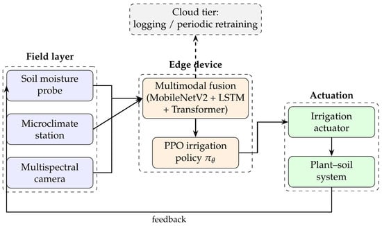
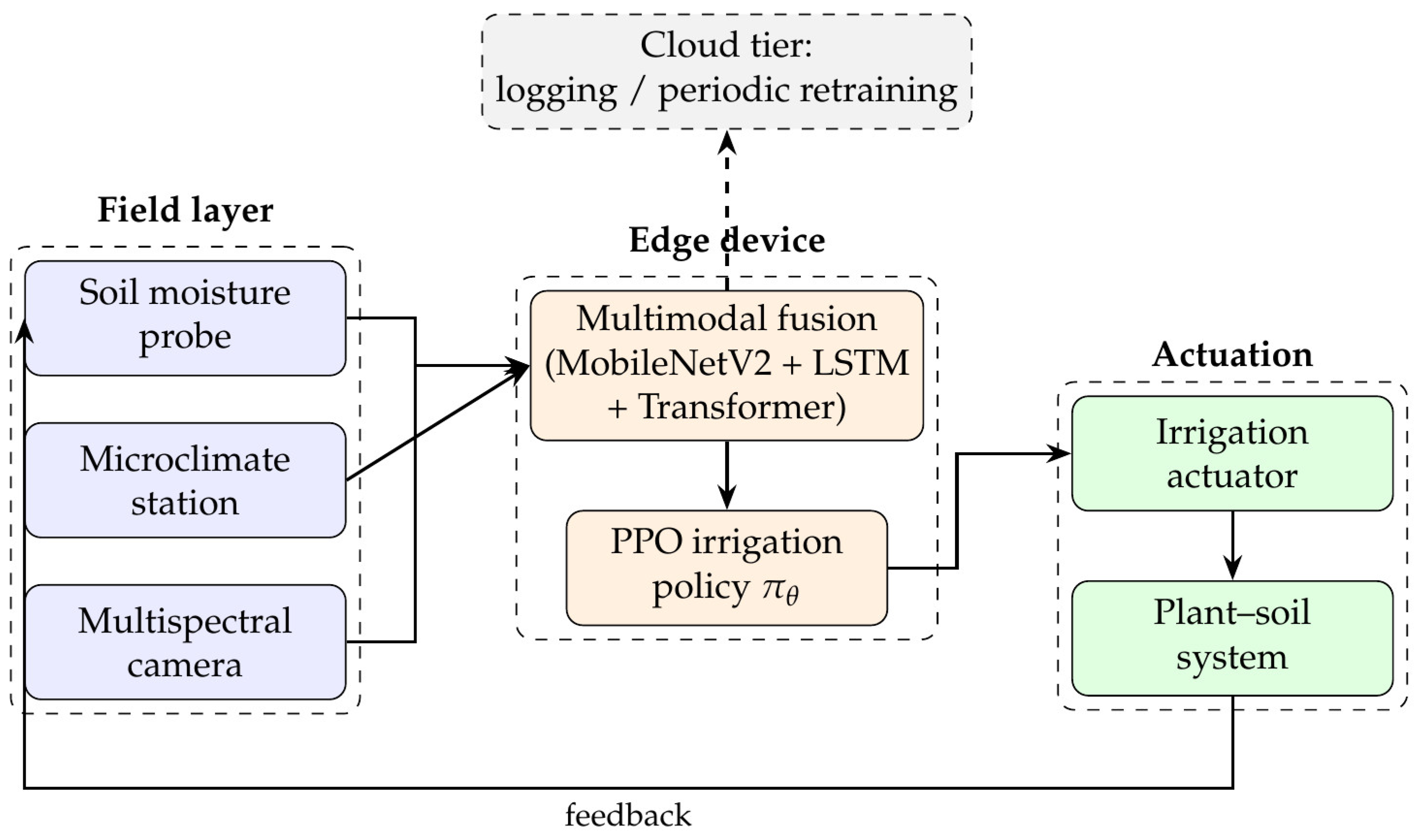
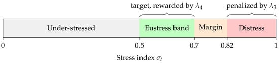
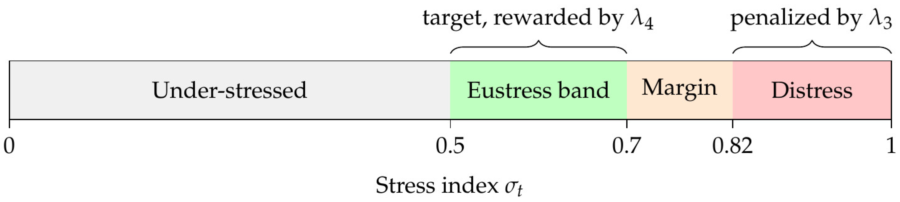
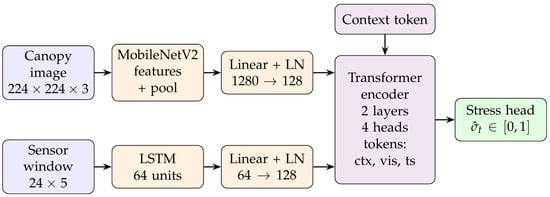
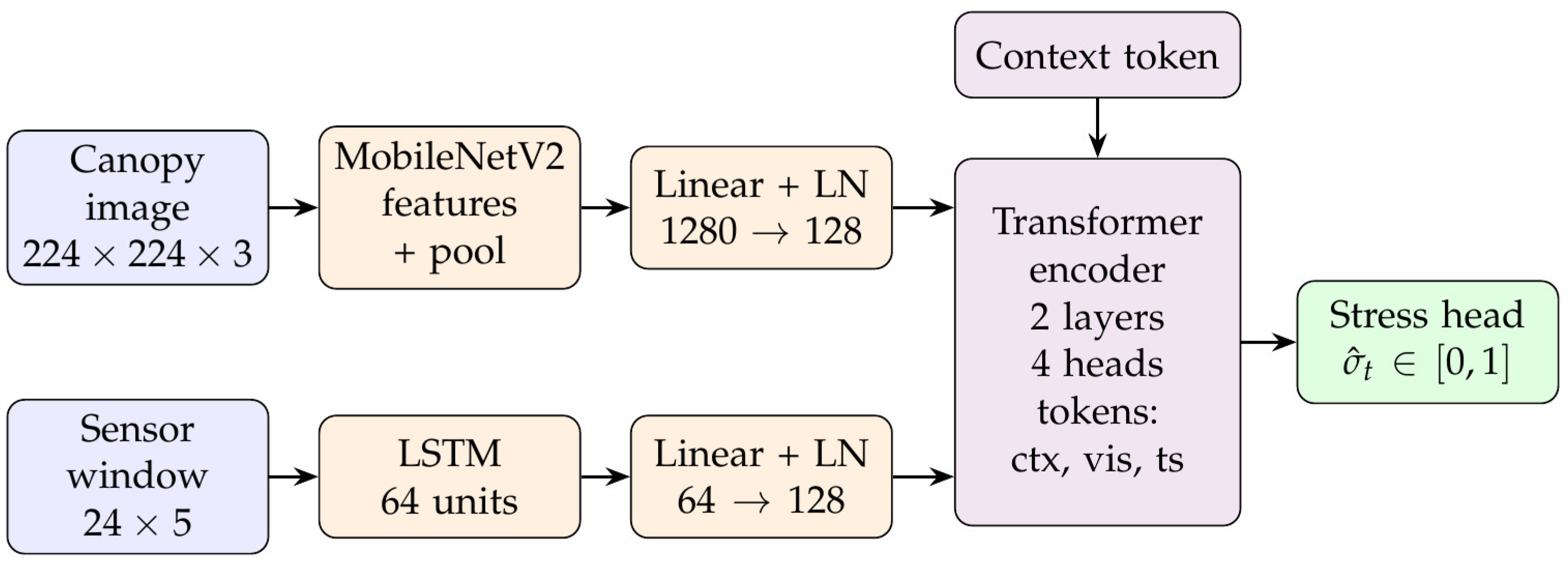
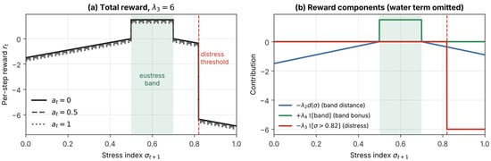
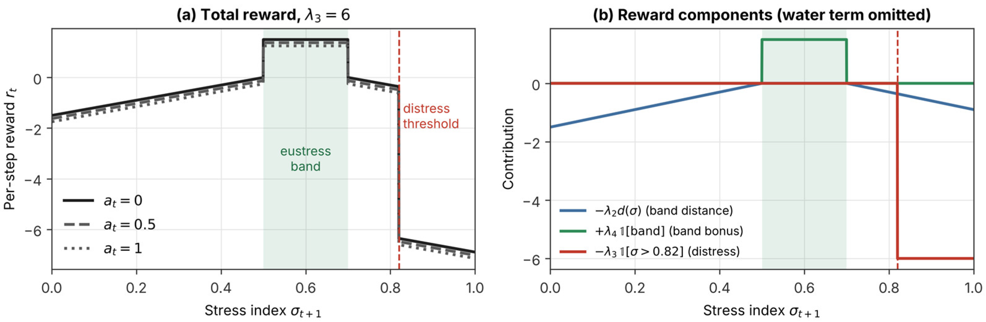
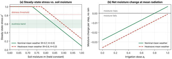
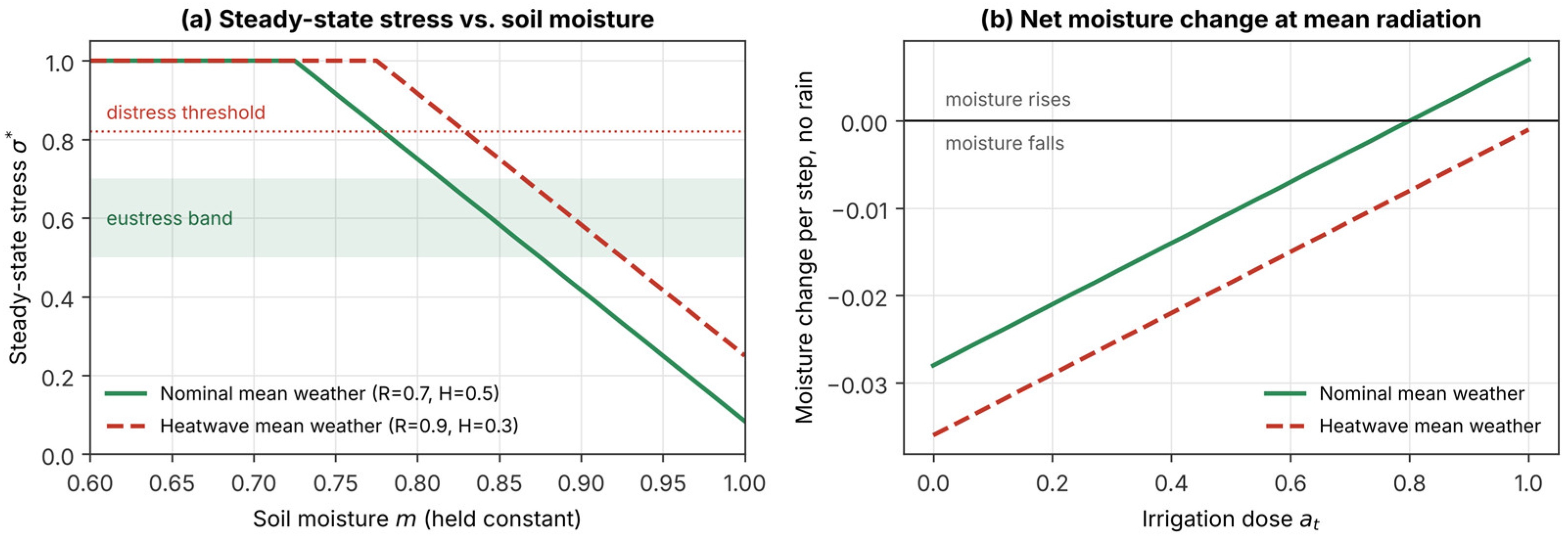
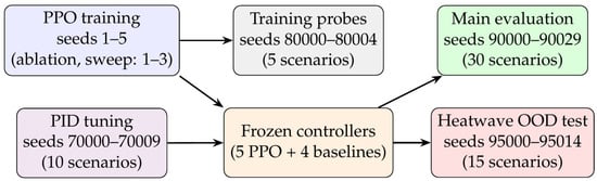
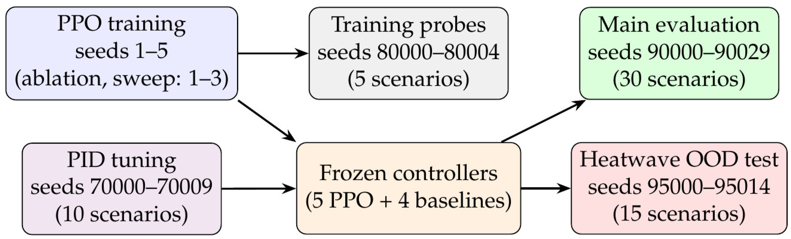
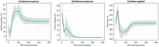
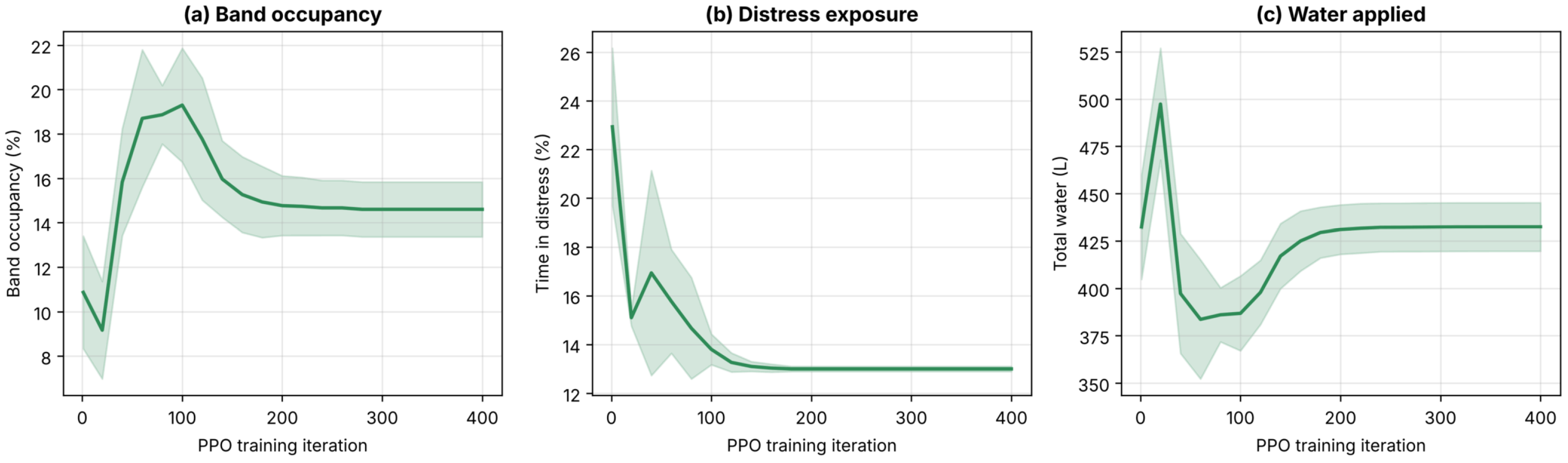
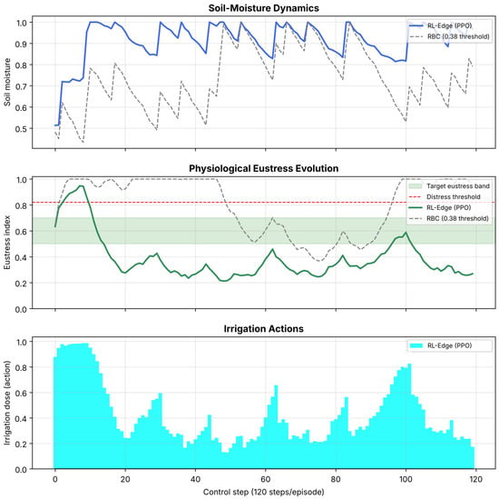
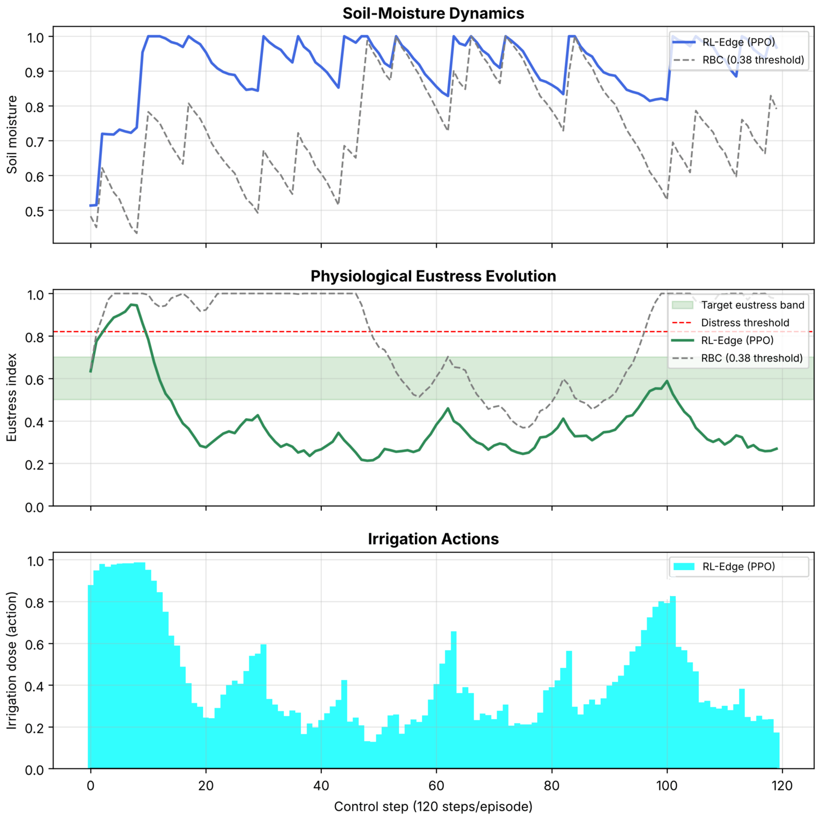
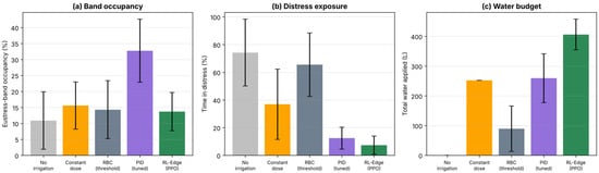
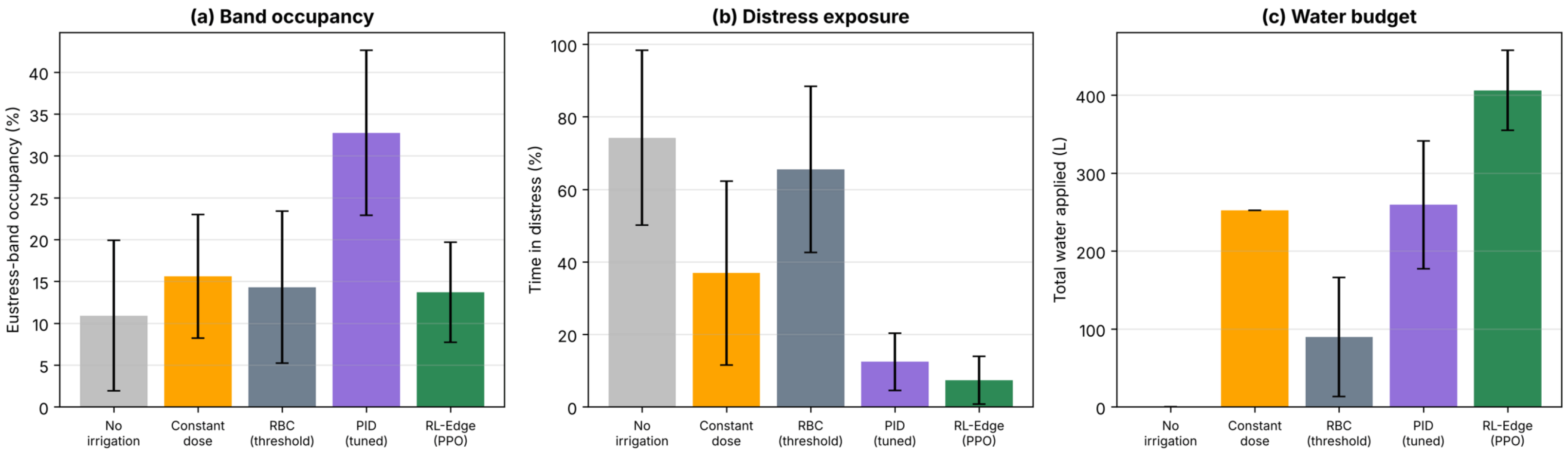
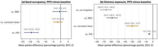
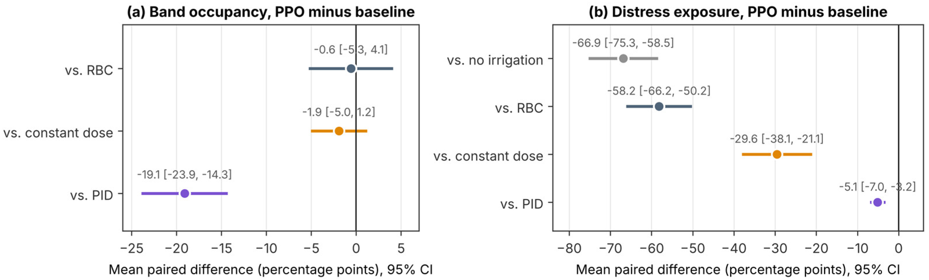
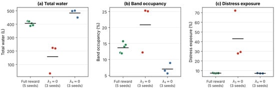
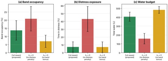
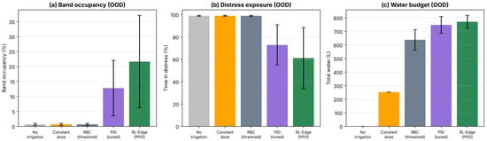
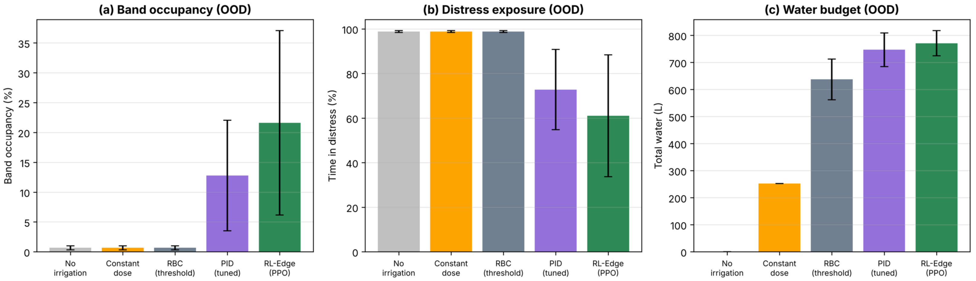
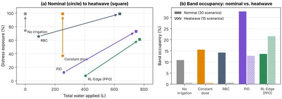
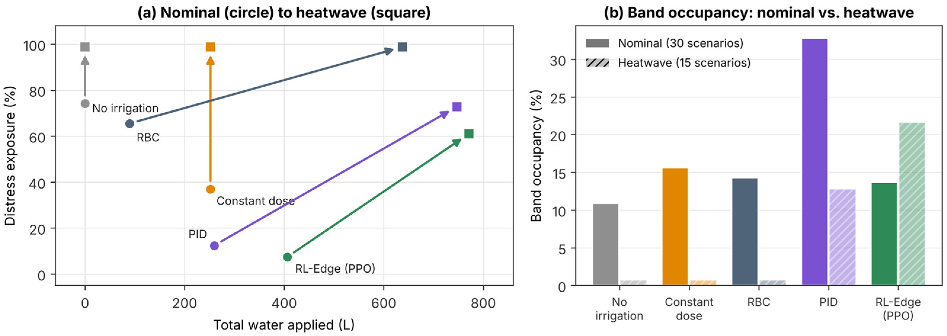
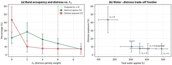
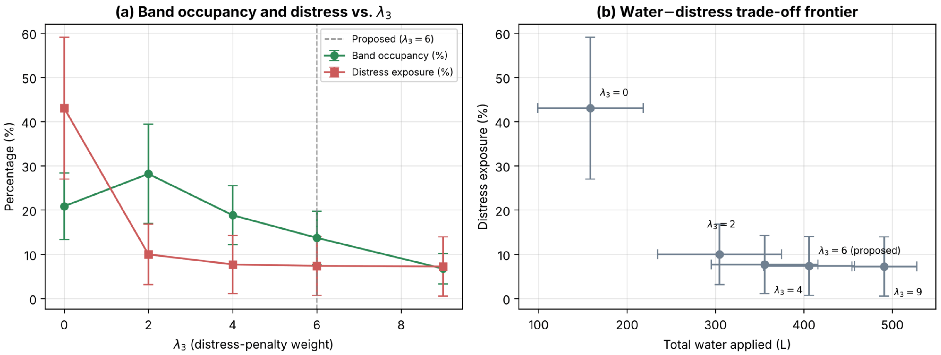

Disclaimer/Publisher’s Note: The statements, opinions and data contained in all publications are solely those of the individual author(s) and contributor(s) and not of MDPI and/or the editor(s). MDPI and/or the editor(s) disclaim responsibility for any injury to people or property resulting from any ideas, methods, instructions or products referred to in the content. |
© 2026 by the authors. Licensee MDPI, Basel, Switzerland. This article is an open access article distributed under the terms and conditions of the Creative Commons Attribution (CC BY) license.