


Abstract
This paper investigates the self-excited longitudinal and torsional vibrations in a driven wheelset operating near the adhesion limit under the nominal traction conditions of an electric locomotive. We develop a unified electromechanical model of the motor–axle system that integrates the induction traction motor’s nonlinear characteristic, a realistic Polach wheel–rail friction law, the wheelset’s longitudinal (rebound) motion, and the first two elastic torsional modes of the axle. The model analyzes the nominal traction operating point, defined by the intersection of the adhesion-limited traction characteristic and the constant-power curve. The results show that electromechanical coupling between electrical slip and wheel–rail creep prevents the traction motor from delivering its rated torque at the nominal speed, making the attainable steady-state torque dependent on the adhesion conditions. Furthermore, a nonlinear stability analysis reveals a Hopf-induced multi-stability structure where an intermediate unstable limit cycle separates two stable cycles—one dominated by rebound motion and the other by torsional vibration. These periodic regimes produce large oscillation amplitudes and reduce both the mean traction force and motor torque, thereby degrading effective tractive performance. Finally, we identify the minimum damping levels required in the drivetrain and steering system to suppress this unstable regime, providing concrete engineering guidance for improving traction behavior near the adhesion limit.
1. Introduction
The continuous demand for higher passenger train speeds and increased haulage capacity in freight transportation requires locomotives and powered rail vehicles capable of delivering progressively higher tractive effort [1]. The safe and efficient generation and utilization of this tractive effort are fundamentally governed by the complex physical phenomena occurring within the wheel–rail contact patch [2,3,4]. This interface is subject to an upper physical limit, commonly referred to as the adhesion limit, which defines the maximum tangential force that can be sustained before gross sliding occurs [5,6]. Efficient exploitation of the available adhesion, particularly under variable environmental conditions (such as moisture or surface contamination) and under high traction demands, remains a major challenge in modern railway engineering [7,8].
Operating the wheelset near the saturation point of the adhesion–slip curve is desirable for maximizing traction. However, this operating region is inherently unstable [9,10]. When the required traction force exceeds the available adhesion, the wheelset begins to slip as the wheel–rail friction force drops beyond the adhesion limit. This reduces the effective traction force that can be delivered and may trigger self-excited vibrations, most notably stick–slip oscillations, in which the wheelset rapidly alternates between adhesion (stick) and sliding (slip) states [11,12,13]. These vibrations are a critical concern, as they induce severe dynamic loads on the drivetrain components [14,15]. Furthermore, this phenomenon contributes substantially to the accelerated wear of both the wheel tread and the rail head, a form of damage often referred to as rail corrugation [16,17,18,19].
Stick–slip oscillations are not specific to the traction mode; they also occur during braking [20] or while curving, where they can produce wheel squeal, which negatively affects passenger comfort [21,22].
The dynamic behavior of a driving wheelset under high traction is a complex, coupled phenomenon. Historically, research has often focused on the torsional (rotational) vibrations of the electromechanical drive system, neglecting the wheelset’s longitudinal motion [23,24,25,26]. Nevertheless, other studies consider the torsional and longitudinal dynamics as inextricably linked motions [27,28], highlighting the importance of coupling effects in high-traction wheelsets. The longitudinal tangential force generated at the wheel–rail contact acts as the critical coupling mechanism between the rotational slip dynamics and the longitudinal oscillations of the entire wheelset assembly [29,30]. This coupling is particularly pronounced during locomotive acceleration or stick–slip events, where the rapid variation in tangential force excites both the rotational modes of the drivetrain and the longitudinal translational modes of the wheelset [31,32,33,34,35].
Several key factors contribute to the initiation and severity of these coupled longitudinal-torsional vibrations. The primary source of excitation is the interaction between the electric motor’s torque characteristics and the highly nonlinear friction characteristics at the wheel–rail contact [36]. These electromechanical interactions, together with the variations in adhesion forces, can generate self-excited torsional vibrations in the drive system [37]. In addition, the internal dynamics of the transmission system itself play a significant role. Rotor eccentricity, for instance, significantly affects the motor bearings [38]. Modern high-speed trains utilize complex gear transmissions, where manufacturing imperfections—such as gear eccentricities—combined with traction torque can introduce significant periodic excitations. This leads to considerable increases in vibration amplitudes within the transmission system, an effect that becomes more pronounced at higher operating speeds [39,40].
Beyond the electromechanical drivers, the mechanical suspension parameters of the bogie play a critical role in mitigating or exacerbating these vibrations. The wheelset is connected to the bogie frame via longitudinal guides, and the traction motor itself is mounted with a certain degree of stiffness. The relationship between these stiffness values is a key determinant of the system’s dynamic response [41]. For instance, it has been shown that the system’s re-adhesion performance—its ability to recover from a slip event—is directly impacted by the longitudinal guide stiffness and the motor suspension stiffness [42]. This study demonstrated that increasing these stiffnesses can enhance the stability of the stick–slip vibration by reducing the amplitude of the slip rate.
The adhesion force itself is not a simple constant, but a dynamic variable influenced by slip speed, contact pressure, and environmental conditions [43,44]. The negative slope of the adhesion–slip curve in the slip region is the fundamental driver of the self-excited oscillations. Therefore, the characteristics of the traction control system, which regulates the slip rate, are closely linked to the mechanical vibrations [45,46]. An improperly tuned anti-slip controller can exacerbate stick–slip behavior, leading to wheel tread wear and fatigue damage, while a delayed response of the wheel slip prevention system may induce dynamic oscillations that accelerate the development of wheel/rail rolling contact fatigue [47,48].
To fully understand and mitigate these longitudinal vibrations, comprehensive models are required. Recent efforts have focused on developing integrated, multi-physics models that couple the multibody dynamics of the vehicle, the electromechanical properties of the traction drive, and sophisticated nonlinear representations of the wheel–rail contact [49,50,51,52]. Such simulations are essential for predicting system behavior under saturated adhesion and for virtually evaluating new mechanical designs or control strategies [53].
Despite significant progress in understanding the stick–slip phenomenon, the current literature still exhibits important gaps in the integrated modeling of driven wheelset dynamics necessary to elucidate the fundamental stability characteristics of this nonlinear phenomenon. In particular, many foundational studies, which focused on exploring the basic properties of stick–slip, consider pure torsional or pure longitudinal vibrations, often simplifying the axle as a rigid body or employing simplified friction laws that fail to capture the full complexity of the self-excitation mechanism. A critical deficiency is the neglect of the explicit, nonlinear coupling between the complex wheel–rail contact dynamics (adhesion model) and the nonlinear mechanical characteristics of the electric traction motor, which serves as the primary source of excitation energy driving the instability. Moreover, existing studies often overlook the dynamic behavior of the wheelset when the locomotive operates throughout its nominal motor operating regime, where the traction characteristic transitions from the adhesion-limited constant force state to the constant power state. This approach fails to capture the complete torsional-longitudinal coupling mechanism that manifests under these crucial operating conditions. Furthermore, the identification and separation of critical mode-related frequencies and the understanding of possible nonlinear multi-stability regimes remain essential open problems for improving traction and railway safety.
In this context, the present work develops a discrete–continuous electromechanical model of the motor–axle system of an electric locomotive. Unlike unpowered trailer wheelsets in railway cars, a locomotive driven wheelset transmits high tractive efforts and sustains heavy axle loads while coupled directly to a traction motor. This electromechanical interaction creates distinct self-excited longitudinal–torsional dynamics near the adhesion limit, which differ fundamentally from the passive rolling behavior of towed vehicles. The proposed model simultaneously captures the longitudinal (rebound) dynamics of the wheelset and the first two elastic torsional modes of the axle, and explicitly couples the nonlinear mechanical characteristic of the induction traction motor with a realistic wheel–rail friction law (Polach). While adhesion-limited phenomena are well established in the literature, the present study addresses them within the nominal traction regime—defined as the operating point where the adhesion-limited curve intersects the constant-power characteristic—an operating condition of practical importance that has received limited attention. Based on the proposed model, it is demonstrated that the interaction between electrical slip and wheel–rail creep prevents the traction motor from delivering its rated torque at the nominal running speed, with the attainable steady-state torque depending strongly on the adhesion conditions (dry or wet rail). The model further enables the investigation of self-excited instabilities arising near the nominal traction point and reveals a multi-stability structure consisting of two stable limit cycles—one dominated by rebound motion and the other by the first torsional mode—separated by an intermediate unstable limit cycle generated through a Hopf bifurcation.
Finally, this study quantifies how the self-excited limit cycles not only introduce significant oscillations in axle rebound, traction force, and motor torque, but also induce an additional reduction in their mean values, compounding the loss already caused by operation beyond the adhesion limit. This results in a net degradation of tractive effort and motor torque. The minimum damping levels required in the drivetrain and guiding system to suppress these detrimental periodic regimes are identified, thereby providing engineering guidelines for improving traction performance near the adhesion limit.
2. Mechanical Model and Governing Equations
The mechanical model of the unilateral drive system of an electric locomotive [54,55], running at constant velocity V on a straight and rigid track, is shown in Figure 1. The drive system consists of the rotor (1) of the traction motor, the driven shaft (2), the pinion (3), the big cogwheel (4), the axle of the driven wheelset (5), the wheels (6), and the axle boxes (7). The moving rigid base (8), representing the bogie chassis, guides the wheelset through a steering system composed of two Kelvin–Voigt systems (9). Each wheel supports a static load Q resulting from the suspended mass of the locomotive, including the wheelset mass itself.
Figure 1.
The mechanical model of the unilateral drive system: 1. rotor; 2. driven shaft; 3. pinion; 4. big cogwheel; 5. axle; 6. wheel; 7. axle box; 8. moving rigid base; 9. steering system.
The axle is modeled as a free-free uniform circular shaft with distributed mass and elasticity, undergoing torsional vibration described by the rotation angle θ(x, t), where x denotes the position along the axle with respect to the reference frame Oxy attached to the axle end near the big cogwheel, and t stands for the time. The rotor, pinion, big cogwheel and wheels are modeled as rigid rotating bodies attached to the axle, with rotation angles denoted θr(t), θp(t), θc(t) = θ(b, t), θ1(t) = θ(a, t), and θ2(t) = θ(l − a, t), where a and b represent the distances from the reference frame to wheel 1 and the big cogwheel, and l is the axle length. In addition to torsion, the wheelset undergoes longitudinal translation (rebound), denoted as y(t).
To isolate the physical mechanisms driving the longitudinal–torsional instability and maintain analytical clarity, the wheelset is restricted to a single translatory degree of freedom y(t). Secondary displacements, such as lateral shifting and yawing, are intentionally omitted to avoid the mathematical overlap with lateral hunting instability (a phenomenon specifically evaluated under running stability standards such as EN 14363 [56]), which is governed by wheel–rail profiles and wheelset conicity rather than the nominal traction dynamics.
The driving source is a three-phase squirrel-cage induction motor operating at the nominal voltage U1 and frequency f. It develops a motor torque T(t) acting on the rotor. From the rotor, this torque is transmitted to the wheels, where wheel–rail creep generates the friction forces between the wheels and rails, F1,2(t).
The parameters associated with the torsional and rebound vibrations are as follows: Mw is the wheelset mass; m = ρS is the axle mass per unit length, where ρ is the material density and S is the area of the mean cross-section; GIp is the torsion stiffness, with G the shear modulus and Ip the polar moment of inertia of the axle section; Jw, Jc, Jp, Jr are the mass moments of inertia of the wheel, big cogwheel, pinion and rotor; ks is the stiffness of the driven shaft including the elastic coupling; 2ky and 2cy are the stiffness and viscous damping of the wheelset steering system; R is the wheel radius; and it is the transmission ratio.
Both wheels are identical and the technological asymmetries are neglected. All rolling surfaces are smooth, without any defect.
The motion of the unilateral drive system components is described as follows. The torsional rotation angle of the wheelset is described using the modal method and retaining the first two elastic torsional modes of the wheelset:
where θ0(t) is the rigid-body rotation of the axle, and [θ1o + Δθ1(t)] and [θ2o + Δθ2(t)] are the modal coordinates, consisting of components θ1o and θ2o (representing the angular offset between the wheels and rotor at equilibrium) and time-dependent coordinates Δθ1(t) and Δθ2(t). The corresponding mode shapes are Θ1(x) = cos (πx/L) and Θ2(x) = cos (πx/L) [57].
The rigid-body rotation θ0(t) consists of three components:
namely (Ω + Ωo)t, the uniform rotation required to transmit the steady torque To; the constant residual angle θ0o between the rotor and axle; and the time-dependent component Δθ0(t). Here, Ω = V/R is the pure rolling speed, and Ωo is the steady slip angular speed required to generate the stationary friction forces.
From Equations (1) and (2), the rotation angles of the wheels and big cogwheel are obtained as follows:
Taking the rotor angle as reference and neglecting the elasticity between the pinion and big cogwheel, the relations for the rotor and pinion rotations become
where it(Ω + Ωo)t corresponds to the equilibrium position, and Δθr(t) is the time-dependent component.
The longitudinal motion of the wheelset is decomposed as
where Vt is the translational motion corresponding to the constant speed V; yo is the steering system deformation under the steady traction force; and Δy(t) is the time-dependent rebound displacement.
Applying Euler’s rotational equations and Newton’s second law, the equations of motion are obtained:
- −
- Equation for the rotor motion:
- −
- Equation for the rigid mode of the axle:
- −
- Equation for the first elastic mode of the axle:
- −
- Equation for the second elastic mode of the axle:
- −
- Equation for the wheelset rebound motion:
Details regarding Equations (18)–(21) are provided in Appendix A.
The equations of motion are completed by the equations for the motor torque and friction forces. Thus, for a three-phase squirrel-cage induction motor, the motor torque is given by the following [58]:
where np is the number of phases, p1 is the number of pole pairs, R1 is the stator resistance, R21 is the rotor resistance referred to the stator, X is the stator reactance, s(t) is the slip, and ηm is the motor efficiency. The time variation in the motor torque arises from rotor speed perturbations introduced through the slip.
The slip is defined as
where is the rotor angular velocity and Ωs = 2πf/p1 is the synchronous angular velocity.
According to Polach’s model [59], the wheel–rail friction forces depend on the wheel creep and on the shear stiffness of the contact:
where Q is the static load on wheel, μi(t) is the friction coefficient at wheel i, and kA, kB are reduction factors for the adhesion and slip regions of the contact ellipse, accounting for dry, wet, or contaminated running surfaces. The quantity εi is Polach’s equivalent creep parameter, depending on the shear stiffness of the contact and on the wheel creep:
where ae, be are the semiaxes of the contact ellipse, C11 is Kalker’s longitudinal coefficient [60] and νi(t) is the creep of the i-th wheel. The ellipse dimensions are calculated using Hertz’s theory for the contact between two elastic solids.
The kinetic friction coefficient is a function of slip velocity of the wheel,
where μs is the coefficient of static friction, Aμ = μ∞/μs, with μ∞ being the limiting friction coefficient at infinite slip velocity, B is the slip velocity factor [s/m], and wi(t) is the slip velocity at wheel i:
The creep of wheel i is the ratio between the slip velocity and the wheel rolling speed,
Within this mathematical framework, the general terms “dry” and “wet” track conditions do not describe ambient humidity but define distinct tribological states. All physical factors—such as rail head roughness, temperature shifts, oxide layers, or moisture—are comprehensively integrated into the specific calibration of the contact parameters (μs, kA, kS, B), whose numerical scaling values are provided later in the paper.
To evaluate the system’s stability and characterize its post-bifurcation behavior, the governing equations are decoupled into a stationary (steady-state) equilibrium regime and a dynamic perturbation regime. The stationary solution establishes the baseline electromechanical operating point, while the remaining time-dependent variations describe the self-excited nonlinear dynamics around this equilibrium position.
Accordingly, the motor torque is decomposed into its steady component To, corresponding to the equilibrium conditions, and the time-dependent perturbation ΔT(t),
Also, the friction force acting on each wheel has a constant component Fo and a perturbed component ΔFi(t),
Setting all time-dependent variables to zero in the equations of motion, the equations of the equilibrium point hold:
where the unknowns are θ0o, θ1o, θ2o, yo and Ωo. The quantity Ωo enters implicitly in To and Fo through the constant component of the slip:
and through the constant component of the wheel creep:
Replacing s(t) with so in Equation (13), the stationary component of the motor torque is obtained:
Similarly, the stationary component of the friction force is as follows:
where the stationary components of the following variables are used:
From Equations (22) and (23), this yields
Equation (32) is nonlinear in Ωo, and its solution can be obtained using the Newton–Raphson method.
Once Ωo is known, the stationary components of the motor torque and friction force are obtained, and the remaining parameters of the equilibrium point can be calculated from the equations of the equilibrium point.
Inserting these results in the equations of motion (8)–(12), the nonlinear equations governing the perturbed motion about the equilibrium point hold:
where the perturbed components of the motor torque, ΔT(t), and friction force, ΔF1,2(t), are derived from Equations (22) and (23).
Although the equations derived above govern the dynamics around any arbitrary equilibrium point, the actual vehicle operation revolves around a specific, highly critical regime: the nominal traction operating point. In railway engineering, this point defines the maximum effective tractive performance of the electric locomotive and serves as the baseline for the subsequent stability and bifurcation analysis.
To formalize this nominal traction regime within the mathematical model, the mechanical characteristic of the asynchronous traction motor is analyzed. The nominal traction operating point corresponds to the nominal torque Ton and the nominal slip, which typically takes the standard value of son = 0.01 for high-power induction traction motors.
Beyond the nominal zone, the motor performance is bounded by the pull-out torque Top and its corresponding pull-out slip sop, which depend strictly on the stator and rotor parameters (the concrete numerical configuration of this characteristic for the analyzed locomotive is detailed later). The operational slip must not exceed sop, as operating beyond this limit induces severe electromechanical instability in the drivetrain.
The mechanical characteristic is used to determine the nominal operating parameters of the locomotive, namely the tractive effort and the nominal speed. To this end, the slip is computed from Equation (14) by setting Ωo = 0 (zero wheel–rail creepage):
where Vs = RΩs/it is the synchronous speed for which both slip and motor torque are zero. Electromagnetically, this corresponds to the rotor speed matching the speed of the rotating magnetic field, so no torque is developed. Because of this fact, the locomotive speed must be lower than the synchronous one.
The corresponding nominal speed of the locomotive (Vn) is then directly governed by the nominal slip relative to the synchronous speed:
Three critical parameters of the driven wheelset are introduced to define the tractive performance under the nominal traction operating point. These parameters are used to quantify the mean value reductions and large oscillation amplitudes detailed in Section 3.
First, the motor torque reduced to the wheelset, Tw(t), accounts for the transmission ratio and is decomposed into its stationary component, Two, and perturbed component, ΔTw(t),
Second, the traction force, Ft(t), representing the actual longitudinal force transmitted to the moving rigid bogie frame, is defined as
where Fto is the stationary component of the traction force and ΔFt(t) is the perturbed component.
Third, the mechanical efficiency of the driven wheelset, η, is established to quantify the power losses induced by wheel–rail creepage at the stationary operating point. This parameter measures the steady-state mechanical power delivered to the bogie frame, Po, relative to the stationary input power received by the wheelset, Pi,
The nonlinear equations of motion describing the perturbed motion about the equilibrium point may exhibit one or more periodic solutions (limit cycles), or even none. The latter occurs when the equilibrium point is asymptotically stable, while limit cycles appear around unstable equilibrium points. These cycles may be stable or unstable, and their properties are investigated by numerically integrating the nonlinear equations of motion (Equations (33)–(37)). This numerical analysis is performed using a fourth-order Runge–Kutta method to evaluate the stability of the steady states and to detect Hopf bifurcations, all of which are detailed and physically characterized in the next section.
3. Results
This section presents a numerical application of the electromechanical model developed above, organized into the parameters of the wheelset drive system and the resulting steady-state and nonlinear stability analyses.
3.1. Model Parameters
The parameter values used in the model are listed in Table 1 and correspond to the drive system of a six-axle LEMA locomotive manufactured by SOFTRONIC (Craiova, Romania), equipped with MTA-ES-108 asynchronous motors rated at 1000 kW.
Table 1.
Parameters for the model of the drive system of the wheelset.
The semiaxes of the contact ellipse were computed for a conical wheel profile and a rail with a circular profile of radius 300 mm.
3.2. Steady-State and Nonlinear Stability Analysis
Based on the drive system parameters defined above, the equilibrium operating points and the self-excited dynamic regimes near the nominal traction point are investigated below.
Figure 2 shows the traction-limited characteristic of the locomotive, which consists of two regions: a straight segment indicating that the locomotive delivers a constant tractive effort limited by the maximum adhesion that can be generated at the wheel–rail contact, and a curved segment corresponding to the constant-power regime.
Figure 2.
Traction-limited characteristic of locomotive [61].
Point N marks the intersection between the two regions and defines the nominal operating parameters of the locomotive: a tractive effort of 292 kN and a nominal speed of 71.4 km/h. The asynchronous motors operate at nominal voltage and frequency, and the slip takes its nominal value. The traction–limit curve is calculated for half–worn wheels of 1210 mm diameter and a transmission ratio of it = 3.478 (80/23); for reference, the limits of the wheel diameter—1250 mm when new and 1170 mm at wear limit—are also indicated. The synchronous speed is 72.1356 km/h.
Figure 3 presents the motor torque reduced to the wheelset, derived from the mechanical characteristic of the asynchronous motor as a function of slip at nominal voltage and frequency. The points corresponding to the nominal and the pull-out torques are indicated. The nominal reduced torque is 29.443 kNm, while the pull-out value is 84.508 kNm, i.e., 2.87 times larger, which is consistent with literature values of approximately 2–3 times the nominal torque [62].
Figure 3.
Motor torque reduced to wheelset: ●, nominal torque; ●, pull-out torque.
As already mentioned, both the traction-limited characteristic and the motor mechanical characteristic assume ideal rolling conditions with no slip between wheels and rail. In reality, however, achieving the traction-limited curve depends on the wheel–rail friction coefficient, which is strongly influenced by wheel creep and varies considerably due to surface contamination, roughness, temperature, humidity, and other factors.
Figure 4 illustrates the effect of wheel creep on the equilibrium point at the nominal speed of 71.4 km/h for both dry and wet running surfaces.
Figure 4.
The effect of the wheel creep on the equilibrium point at 71.4 km/h.
The two terms of the nonlinear equilibrium Equation (40)—the motor torque reduced to wheelset (Tw) and the torque of the friction forces (2RFo)—are shown. The friction torque is computed using the dry and wet friction parameters listed in Table 1. The intersection of the curves determines the equilibrium point.
For dry running surfaces, the reduced motor torque is 24.465 kNm at a creep of 0.2023%. For wet surfaces, the reduced torque drops considerably to 15.640 kNm, while the creep rises to 0.5113%. Both torque values are below the nominal reduced torque of 29.442 kNm derived from the traction characteristic. This happens because the traction characteristic is computed under idealized assumptions that neglect the influence of the wheel creep on motor slip. Since wheel creep—without which the traction cannot develop—reduces motor slip, the torque transmitted to the wheelset becomes lower than the ideal value predicted by the traction characteristic.
A natural question is under which conditions the motor torque reduced to wheelset attains its nominal value. To compensate for the slip reduction caused by creep, the wheelset rotational speed—and therefore the locomotive speed—must decrease. For example, Figure 5 shows that at 71.224 km/h (dry conditions), the reduced motor torque matches the nominal value of 29.443 kNm, corresponding to a creep of 0.267%.
Figure 5.
The effect of the wheel creep on the equilibrium point at 71.224 km/h (dry running surfaces).
The deviation from the ideal nominal speed (71.4 km/h) is very small. Figure 6 shows the locomotive speed at which the motor develops nominal torque for different maximum friction coefficients ranging between 0.3 and 0.5 (dry/wet conditions). The curves result from the intersection of the friction–torque curve for a given maximum friction coefficient with the nominal reduced torque of 29.443 kNm.
Figure 6.
Speed at nominal torque.
The reduced motor torque reaches its nominal value at progressively lower speeds as the maximum friction coefficient decreases toward the adhesion limit. For dry surfaces, the nominal–torque speed drops from 71.224 km/h at μs = 0.55 to 70.0914 km/h at the adhesion limit (μs = 0.307). For wet surfaces, the effect is much stronger: the nominal–torque speed decreases from 70.71 km/h to 66.41 km/h as μs decreases to 0.3217. These results are confirmed in Figure 7, which shows the intersection of the reduced motor torque and friction torque curves at the adhesion limit, both yielding the nominal torque for dry and wet conditions.
Figure 7.
Nominal torque at the adhesion limit: (a) dry running surfaces, V = 70.0914 km/h, μs = 0.3074; (b) wet running surfaces, V = 66.4077 km/h, μs = 0.3217; color code as in Figure 5.
The variation in the mechanical efficiency of the wheelset follows the same pattern as the nominal torque speed curves (Figure 8). Under dry conditions, the efficiency remains above 0.9815, whereas under wet conditions it may drop to 0.9299, becoming lower than the efficiency of the asynchronous traction motor itself.
Figure 8.
The mechanical efficiency of the wheelset when running on dry/wet surfaces developing nominal torque.
Once all parameters of the equilibrium point have been determined, the stability analysis can proceed.
However, some preliminary observations are important regarding the couplings between the various components of the drive system. The torsional vibration of the axle is coupled to the rebound vibration only through the friction forces; without them, the two vibrations remain obviously decoupled. Similarly, the torsional vibration of the wheelset is coupled to that of the rotor through the reduction gear.
Table 2 presents the natural frequencies for the vibration modes of the system in two states: when the wheelset is disconnected from the motor (it = 0) and when the wheelset is connected (it = 3.478). The first column details the decoupled modes: axle torsion at 60.66 and 503.75 Hz, the wheelset rebound at 19.87 Hz, and rotor torsion at 12.51 Hz. The coupling between the wheelset and the rotor through the drive gear stiffens the drive system. This is evident from the increase in natural frequencies shown in the second column (it = 3.478): the axle torsion modes rise to 62.33 and 510.31 Hz, and the rotor frequency increases to 22.52 Hz.
Table 2.
Natural frequencies.
Next, the stability of the equilibrium points, where the motor develops nominal torque, is analyzed for different running surface conditions. Damping in the wheelset steering system and driven shaft is neglected.
Figure 9 and Figure 10 illustrate the wheelset rebound vibration around the equilibrium point when the motor develops nominal torque on dry running surfaces, using different maximum friction coefficients and locomotive speeds: μs = 0.55 and V = 71.2241 km/h (Figure 9), and μs = 0.35 and V = 70.9328 km/h (Figure 10). Initially, all state variables have zero deviation from the equilibrium values, except for the rebound displacement, which has a deviation of 1% × yo. As the maximum friction coefficient is reduced, the equilibrium point approaches the adhesion limit, as shown in diagrams (a) of Figure 9 and Figure 10. In all considered situations, the motion around the equilibrium point is damped, indicating that the equilibrium point is asymptotically stable. However, the damping of free vibrations decreases progressively as the equilibrium point approaches the adhesion limit, an aspect highlighted by comparing diagrams (b) of these figures.
Figure 9.
The stability of the equilibrium point at the nominal torque for V = 71.2241 km/h and μs = 0.55 (dry running surfaces): (a) equilibrium point; color code as in Figure 5; (b) wheelset rebound.
Figure 10.
The stability of the equilibrium point at the nominal torque for V = 70.9328 km/h and μs = 0.35 (dry running surfaces): (a) equilibrium point; color code as in Figure 5; (b) wheelset rebound.
When the wheelset runs at the adhesion limit, it is at the stability limit, as shown in Figure 11. Numerically, highlighting this stability limit is challenging. Based on several numerical experiments, the following parameter configuration was determined: maximum friction coefficient μs = 0.307365 and locomotive speed V = 70.10097 km/h. It is observed that the wheelset rebound vibration tends to maintain its amplitude, which indicates, from the perspective of stability theory, that the steady state is simply stable.
Figure 11.
The stability of the equilibrium point at the nominal torque at the adhesion limit, V = 70.10097 km/h and μs = 0.307365 (dry running surfaces): (a) equilibrium point; color code as in Figure 5; (b) wheelset rebound.
To verify the calculation accuracy, the numerical simulation of the vibration behavior must be run for a longer duration. Figure 12 shows two 20 s sequences of the rebound vibration: one at the speed mentioned above, and the second at V = 70.10096 km/h. At V = 70.10097 km/h the equilibrium is asymptotically stable, while at V = 70.10096 km/h it is unstable.
Figure 12.
Wheelset rebound at the adhesion limit for dry running surfaces (μs = 0.307365): (a) V = 70.10097 km/h—asymptotically stable; (b) V = 70.10096 km/h—unstable.
For wet running surfaces, similar results are obtained, as can be seen in Figure 13 and Figure 14. The same maximum friction coefficient values (μs = 0.55 and μs = 0.35) were used as in the previous case, corresponding to nominal torque speeds of V = 70.7122 km/h and V = 68.9634 km/h, respectively.
Figure 13.
The stability of the equilibrium point at the nominal torque for V = 70. 7122 km/h and μs = 0.55 (wet running surfaces): (a) equilibrium point; color code as in Figure 5; (b) wheelset rebound.
Figure 14.
The stability of the equilibrium point at the nominal torque for V = 68.9634 km/h and μs = 0.35 (wet running surfaces): (a) equilibrium point; color code as in Figure 5; (b) wheelset rebound.
Figure 15 shows the equilibrium point at the adhesion limit and the perturbed vibration for wet running surfaces. Here, the maximum friction coefficient is μs = 0.32173, and the speed at which the nominal torque is developed is V = 66.57 km/h. The vibration exhibits a regular motion with constant amplitude, indicating that the equilibrium point is simply stable.
Figure 15.
The stability of the equilibrium point at the nominal torque at the adhesion limit, V = 66.56882 km/h and μs = 0.32173 (wet running surfaces): (a) equilibrium point; color code as in Figure 5; (b) wheelset rebound.
Furthermore, keeping the speed constant, when the maximum friction coefficient decreases for some reason, the stationary behavior migrates to the right portion of the adhesion limit, as shown in Figure 16a. In this situation, the motor torque at the wheelset is lower than the nominal one, specifically To = 24.361 kNm. Diagram (b) shows the wheelset rebound when it starts with an initial deviation of 1% from the stationary displacement; the zero rebound displacement value corresponds to the wheelset’s equilibrium point, yo = 1.00665 mm. The system’s response to this initial deviation is a vibration that gradually increases until its amplitude stabilizes. This indicates that while the equilibrium point is unstable, the homogeneous nonlinear equations describing the movement around it possess a periodic solution—the limit cycle.
Figure 16.
The equilibrium point beyond the adhesion limit and the limit cycle at V = 70.10097 km/h and μs = 0.25 (dry running surfaces): (a) Equilibrium point:  , motor torque at wheelset;
 , torque of the friction forces;
 , effective torque; (b) limit cycle (initial rebound of 1% × yo).
, motor torque at wheelset; , torque of the friction forces; , effective torque; (b) limit cycle (initial rebound of 1% × yo).
The stability/instability of the equilibrium point, as well as the existence of the limit cycle, can be explained by examining the friction force curve as a function of the slip speed (Figure 17). This curve is equivalent to the friction force vs. creep curve for a given wheelset speed, as slip speed equals the product of the wheelset speed and creep. The friction force curve has a maximum corresponding to the adhesion limit (L), which separates the upward branch (OAL) from the downward branch (LBC).
Figure 17.
An explanatory diagram of the positive/negative damping effect of the friction force versus slip speed.
As shown, the equilibrium point is established when the motor torque at the wheelset equals the torque of the frictional forces. Any perturbation in the wheelset drive system’s configuration relative to a specific equilibrium position results in a variable component of the friction force that overlaps the stationary component. Mathematically, this is reflected by the first two terms in the Taylor series expansion of the friction force function.
When the equilibrium point is on the ascending branch of the friction force curve (e.g., point A), its derivative with respect to the sliding speed is positive. In this case, the dynamic component of the friction force dissipates mechanical energy from the system (positive damping). Consequently, the equilibrium point on this branch is asymptotically stable.
Conversely, when the equilibrium point is on the downward branch (e.g., point B), the curve’s slope is negative. Here, the dynamic component of the friction force introduces energy into the system, causing the amplification of vibrations around the equilibrium point. This variation in frictional force is termed the negative damping effect. Consequently, the equilibrium point on the descending branch of the friction force curve is unstable.
However, the vibration around an unstable equilibrium point does not increase continuously; instead, it settles into a periodic vibration (a limit cycle) during which the friction force takes values around the adhesion limit on both branches of the curve. Starting from the unstable equilibrium point, the amplitude increases continuously at each cycle due to negative friction until the adhesion limit is exceeded. Beyond this point, the frictional force begins operating on the ascending branch, dissipating part of the energy accumulated during the evolution on the descending branch. The vibration thus has two phases corresponding to the time intervals when the frictional force works on the ascending and descending branch, respectively. The vibration amplitude stabilizes when the energy balance between the accumulation (descending branch) and dissipation (ascending branch) is reached [63,64].
If the equilibrium point coincides with the adhesion limit, any perturbation develops on both ascending and descending branches. Thus, an energy balance is established between the energy received and the energy lost through the action of the dynamic component of the force of friction. This condition ensures that the vibration around the adhesion limit will always have a constant amplitude. As a result, the equilibrium point at the adhesion limit is simply stable.
It should also be noted that system vibrations inherently require the presence of at least one elastic element within the kinematic structure.
The periodic nature of the vibration around the previously considered unstable equilibrium point (see Figure 16) can be highlighted using both time-domain and phase-plane representations of the state variables. To achieve this, the time simulation is performed over a 100 s sequence, which is considered sufficient to ensure good numerical periodicity of the results. Thus, Figure 18 shows the wheelset rebound and the time-dependent coordinates corresponding to the two elastic eigenmodes of torsional vibration. The mean value appears on each time series representation. The phase trajectories are closed curves, which confirms the periodic character of the vibration. The period of this limit cycle equals the rebound period, and for this reason, it is termed the limit cycle of rebound.
Figure 18.
Limit cycle of rebound: (a) time series of the wheelset rebound; (b) phase portrait of the wheelset rebound; (c) time series of the first coordinate of the wheelset torsion; (d) phase portrait of the first coordinate of the wheelset torsion; (e) time series of the second coordinate of the wheelset torsion; (f) phase portrait of the second coordinate of the wheelset torsion; (a,c,e) , instantaneous value; ━ ━ ━, mean value.
, instantaneous value; ━ ━ ━, mean value.
The time series associated with the state variables in Figure 18 represent the perturbation relative to the equilibrium point. The non-zero mean value indicates that the vibration is not centered on the unstable equilibrium point; in other words, the resulting limit cycle ‘slips’ relative to it. This phenomenon occurs because the nonlinearity is asymmetric, an aspect well documented in the literature [65,66].
Although the mechanical structure of the drive axle is asymmetric due to the unilateral transmission, this has very little influence on the distribution of frictional forces on the two wheels within the proposed model.
Figure 19 shows the friction forces at the periphery of the wheels over a single period to make the differences between them more easily visible. The two forces evolve in phase and have very close values. The biggest difference between the two friction forces is identified in the zone of their minimum values, but it is insignificant: 18.625 kN at wheel 1 and 18.612 kN at wheel 2. This difference is primarily generated by the first elastic mode of the axle torsion, which, however, has a much smaller influence than that of the rigid mode of vibration. It should be noted that this quasi-identical distribution is also a consequence of the model’s structural assumptions (Equation (22)), where the normal wheel–rail load Q is assumed to remain constant and equally shared between the wheels, thereby isolating the purely torsional effects from dynamic wheel load variations.
Figure 19.
Limit cycle of rebound—friction forces: (a) friction forces. (b) , wheel 1; , wheel 2.
, wheel 1; , wheel 2.
The slip effect of the limit cycle results in a decrease in the mean motor torque at the wheelset compared to the equilibrium point value (Figure 20). The mean torque is 23.681 kNm, versus 24.361 kNm at the equilibrium point. The spectrum of the motor torque at wheelset is dominated by the fundamental component arising at 19.84 Hz. This value is very close to the nominal natural frequency of the wheelset rebound (19.87 Hz), with the minor shift being driven by system damping and the specific nonlinear traction conditions. Its amplitude is 0.224 kNm, representing 0.944% of the mean value.
Figure 20.
Limit cycle of rebound—motor torque at the wheelset: (a) time series: , instantaneous value; ━ ━ ━, mean value; ━ ━ ━, value corresponding to the equilibrium point. (b) Spectrum.
, instantaneous value; ━ ━ ━, mean value; ━ ━ ━, value corresponding to the equilibrium point. (b) Spectrum.
The slip effect of the limit cycle is also evident at the traction force level. Figure 21 shows the time series and spectrum of the traction force variation. The mean value is negative, −1.066 kN, indicating a reduction in traction force relative to the equilibrium point. Moreover, the traction force variation amplitude is very large. This is explained by the fact that the fundamental frequency of the limit cycle is practically equal to the natural frequency of the rebound vibration. In other words, the rebound is operating in resonance. The amplitude of the fundamental harmonic of the traction force reaches 88.27 kN.
Figure 21.
Limit cycle of rebound—variation in the traction force: (a) time series: , instantaneous value; ━ ━ ━, mean value. (b) Spectrum.
, instantaneous value; ━ ━ ━, mean value. (b) Spectrum.
The existence of the limit cycle is justified by the energy balance over one period between accumulated and dissipated energy, achieved through the dynamic component of the friction force (which provides positive or negative damping depending on the operating branch). Figure 22 illustrates this aspect, presenting the two friction forces on the wheels as functions of the sliding speed. For consistency with the representation of the friction force as a function of the sliding speed (see Figure 17), the modulus of the sliding speed is used.
Figure 22.
Friction forces as a function of slip speed: (a) wheel 1; (b) wheel 2.
The results for the two friction forces are similar: both forces operate more extensively in the unstable zone of the diagram than in the stable zone. This is because the effectiveness of the negative damping is lower (the absolute value of the slope is smaller in the unstable zone). The minimum friction force values occur in the stable zone and are explicitly mentioned in Figure 22. The maximum friction force value, obviously, corresponds to the adhesion limit.
The rebound limit cycle is not the only periodic solution existing around the analyzed unstable equilibrium point. Figure 23 shows the rebound vibration when the initial longitudinal displacement of the wheelset is 0.1% × yo. A different evolution is observed: after an initial phase of amplification, the wheelset rebound amplitude gradually decreases until it stabilizes in a limit cycle.
Figure 23.
Limit cycle at V = 70.10097 km/h and μs = 0.25 (dry running surfaces) for an initial rebound of 0.1% × yo.
Figure 24 shows sequences of the numerical simulation that illustrate the transformations through which the wheelset rebound motion evolves until it is transformed into a limit cycle. Initially, the vibration has a regular, harmonic appearance at approximately 19.8 Hz, with slow amplitude modulation (increasing or decreasing; Figure 24a–c). Notably, throughout this start-up period, the movement frequency equals the rebound limit cycle frequency analyzed previously. Diagram (c) shows the motion beginning to change, a phenomenon better understood from diagrams (d) and (e), where a wave with a frequency six times higher than the initial wave emerges. Diagram (f) shows an amplitude-modulated vibration in which the emergent component increases progressively.
Figure 24.
Stages of the metamorphosis of the rebound movement: (a) 0–0.2 s; (b) 5.8–6.0 s; (c) 9.0–9.2 s; (d) 11.0–11.2 s; (e) 13.0–13.2 s; (f) 16.0–16.2 s.
Finally, the limit cycle shown in Figure 25 is reached, whose amplitude is much smaller than that of the rebound limit cycle. The frequency of this limit cycle is 62.1 Hz, a value shifting slightly from the linear natural frequency of 62.33 Hz due to the nonlinear electromechanical coupling. By convention, this limit cycle is called the limit cycle of torsion.
Figure 25.
Limit cycle of torsion (62.1 Hz): (a) The time series of the wheelset rebound: , instantaneous value; ━ ━ ━, mean value. (b) A phase portrait of the wheelset rebound.
, instantaneous value; ━ ━ ━, mean value. (b) A phase portrait of the wheelset rebound.
Figure 26 shows the time coordinates of axle’s torsional elastic modes during the limit cycle of torsion. The time diagrams also display the mean values, which confirm the sliding effect of the limit cycle relative to the unstable equilibrium point (also seen in the wheelset rebound diagram; see Figure 23 and Figure 25a). While the rebound clearly has two major spectral components, the time evolution of the coordinates of the two torsional vibration modes is practically in the form of harmonics at the limit cycle frequency. This is a somewhat reversed situation compared to the rebound limit cycle (Figure 18a).
Figure 26.
Limit cycle of torsion: (a) The time series of the first coordinate of the wheelset torsion: , instant value; ━ ━ ━, mean value. (b) A phase portrait of the first coordinate of the wheelset torsion. (c) The time series of the second coordinate of the wheelset torsion: , instantaneous value; ━ ━ ━, mean value. (d) A phase portrait of the second coordinate of the wheelset torsion.
, instant value; ━ ━ ━, mean value. (b) A phase portrait of the first coordinate of the wheelset torsion. (c) The time series of the second coordinate of the wheelset torsion: , instantaneous value; ━ ━ ━, mean value. (d) A phase portrait of the second coordinate of the wheelset torsion.
In the case of the torsional limit cycle, the axle motion is dominated by its first elastic torsional mode, which is an antisymmetric mode. Consequently, the wheels rotate in antiphase, as shown by the variation in the wheel rotation speeds in Figure 27. As a result, the friction forces on the two wheels are different (Figure 28), a behavior that contrasts with the rebound limit cycle (see Figure 19).
Figure 27.
Limit cycle of torsion—variation in the angular speeds.
Figure 28.
Limit cycle of torsion—friction forces.
Figure 29 shows the time series and amplitude spectrum of the motor torque at the wheelset, including the mean value and the unstable equilibrium point value. A reduction of 0.634 kNm in the mean motor torque is observed due to the limit cycle slip effect. The amplitude spectrum is dominated by the fundamental harmonic, whose frequency is 61.7 Hz—a value very close to that obtained via approximate calculation based on the torque’s time representation. The fundamental harmonic amplitude is 4.89% of the continuous component’s value. The other harmonics have much smaller amplitudes, below 1% of the fundamental’s amplitude value. At 1.161 kNm, the fundamental amplitude is significantly larger than the fundamental from the rebound limit cycle (0.224 kNm).
Figure 29.
Limit cycle of torsion—motor torque at wheelset: (a) Time series: , instantaneous value; ━ ━ ━, mean value; ━ ━ ━, stationary value. (b) Spectrum.
, instantaneous value; ━ ━ ━, mean value; ━ ━ ━, stationary value. (b) Spectrum.
Figure 30 shows the variation in the traction force relative to the unstable equilibrium point value, along with the amplitude spectrum. The reduction in the traction force due to the slip effect of the torsion limit cycle is 1.049 kN. The variation in the traction force is much lower compared to that observed in the case of the rebound limit cycle. The most important component of the amplitude spectrum is the second-order harmonic, whose amplitude is 0.0302 kN.
Figure 30.
Limit cycle of torsion—variation in the traction force: (a) Time series: , instantaneous value; ━ ━ ━, mean value. (b) Spectrum.
, instantaneous value; ━ ━ ━, mean value. (b) Spectrum.
By taking slightly different initial conditions, the dynamic regime of the drive axle is found to evolve toward either the rebound limit cycle or the torsion limit cycle. Since these two limit cycles are stable periodic solutions of the nonlinear equations of motion, the transition between them theoretically requires the existence of an unstable limit cycle. The search for this limit cycle is illustrated in Figure 31, which shows the time evolution of the wheelset rebound from extremely close initial displacement values: Δyo(0) = 9.25535072973352 μm and Δyo(0) = 9.25535072973353 μm. In both cases, before reaching the final stable limit cycle, the vibration takes the form of an intermediate periodic movement sustained for approximately 20 s.
Figure 31.
Search for the unstable limit cycle: (a) time series of the rebound for the initial rebound of 9.25535072973352 μm; (b) phase portrait of the torsional limit cycle; (c) time series of the rebound for the initial rebound of 9.25535072973353 μm; (d) phase portrait of the rebound limit cycle.
It is reasonable to consider the periodic movement highlighted above as the unstable limit cycle. Figure 32 shows a short sequence of the wheelset rebound and its spectrum. Practically, the unstable limit cycle takes the form of a harmonic wave with a frequency equal to the natural rebound frequency (19.8 Hz) and exhibits a slight shift in the mean value.
Figure 32.
Unstable limit cycle—wheelset rebound: (a) Time series: , instantaneous value; ━ ━ ━, mean value. (b) Spectrum.
, instantaneous value; ━ ━ ━, mean value. (b) Spectrum.
From the above, it follows that the free vibration of the undamped wheelset drive system around the considered unstable equilibrium point can result in either the rebound limit cycle or the torsional limit cycle, depending on the initial energy.
Next, the influence of damping, expressed as the damping ratio of the steering system,
and of the driven shaft,
on the existence of the two limit cycles is investigated using the previous case as an example.
First, only the influence of the steering system damping (ζy) is considered; the driven shaft damping (ζθ) is set to zero. The Hopf bifurcation diagram is constructed by representing the absolute value of the wheelset rebound extremes corresponding to the limit cycles as a function of the steering system damping ratio. Figure 33 shows the Hopf diagram when (ζy) ranges from 0 to 0.1.
Figure 33.
The Hopf bifurcation diagram—the influence of the damping of the steering system (V = 70.10097 km/h, μs = 0.25, dry running surfaces and ζθ = 0): (a) rebound and torsion limit cycles (0 ≤ ζy ≤ 0.01): ×, rebound; ×, torsion; (b) torsion limit cycle (0.001 ≤ ζy ≤ 0.1).
In Figure 33a, the amplitude of the rebound limit cycle is gradually reduced as the steering system damping increases from zero until the rebound limit cycle overlaps on the unstable limit cycle.
To support this, Figure 34 presents the results when the degree of damping ζy takes the values of 0.41% and 0.42%. For these cases, the initial rebound is ten times greater than the equilibrium point value, and the simulation time is 150 s. Figure 34a shows that the vibration takes the shape of the rebound limit cycle for ζy = 0.41%. When the degree of damping is slightly higher, at ζy = 0.42%, Figure 34b describes a different scenario: the vibration appears to stabilize at the rebound limit cycle for a long time but then begins to decrease continuously, finally evolving into the torsion limit cycle.
Figure 34.
Rebound time series at bifurcation point: (a) ζy = 0.41%; (b) ζy = 0.42%.
Returning to Figure 33a, the rebound limit cycle does not occur for damping ratio values greater than 0.42%. Conversely, the torsional limit cycle can occur for any damping value in the domain considered and its amplitude remains practically constant, as shown in Figure 33a,b. Therefore, the Hopf diagram based on the steering system damping has a bifurcation point for 0.41% < ζy < 0.42%.
Second, only the influence of the driven shaft damping (ζθ) on the two limit cycles is presented ζy = 0). Figure 35 shows the Hopf bifurcation diagram when the damping ratio ζθ ≤ 0.1. The rebound limit cycle is less influenced by the driven shaft damping, showing only a slight amplitude increase in the range considered. The amplitude of the torsion limit cycle decreases as the damping ratio ζθ increases until this limit cycle disappears. The bifurcation point is located in the damping ratio range between 0.011 and 0.012.
Figure 35.
The Hopf bifurcation diagram—the influence of the damping of the driven shaft (V = 70.10097 km/h, μs = 0.25, dry running surfaces and ζy = 0): (a) rebound and torsion limit cycles (0.001 ≤ ζθ ≤ 0.02): ×, rebound; ×, torsion; (b) rebound limit cycle (0.001 ≤ ζθ ≤ 0.1).
Both the elastic coupling and the axle steering system utilize rubber as their base material; therefore, it is reasonable to consider the case where the damping ratios are equal (ζy = ζθ). Figure 36 shows the Hopf bifurcation diagram when the two damping ratios vary from 0.001 to 0.1. It is recalled that the steady-state regime around which the stability of periodic solutions is studied is unstable.
Figure 36.
The Hopf bifurcation diagram—the influence of the damping of the steering system and driven shaft (V = 70.10097 km/h, μs = 0.25, dry running surfaces and ζy = ζθ): ×, rebound; ×, torsion.
When the damping ratios are up to 0.0048, the free vibration of the axle drive system can result in either of the two limit cycles. For damping ratios between 0.0049 and 0.021, the free vibration is only a torsion limit cycle. Importantly, for damping ratios greater than 0.022, both limit cycles disappear, and the steady-state regime becomes stable. This remarkable result confirms the capacity of synchronized mechanical damping to completely suppress the self-excited instabilities near the nominal traction operating point.
4. Conclusions
This paper has investigated the dynamic behavior of a discrete-continuous mechanical model of a wheelset unilateral drive system in an electric locomotive equipped with asynchronous motors. The primary objective was to characterize the dynamic response of the drive system when the motor is supplied at nominal voltage and frequency, develops nominal torque, and the locomotive operates near the adhesion limit on dry and wet rail conditions.
The proposed model incorporates all essential drivetrain components, including the motor rotor, driven shaft, pinion, big cogwheel, axle with the two wheels, axle boxes and the wheelset steering system. The model accounts for the following motions: rotor rotation, wheelset torsional dynamics (including the rigid-body mode and the first two elastic torsional modes), and wheelset rebound translation. The wheel–rail friction forces are described using Polach’s adhesion model. By restricting the analysis to these longitudinal-torsional couplings, lateral displacements and yawing oscillations were omitted to isolate the self-excited adhesion mechanisms from lateral hunting instability.
Equilibrium operating points were determined for various parameter configurations, including running speed and adhesion conditions, and the periodic solutions (limit cycles) developing around these equilibrium points were systematically analyzed.
The steady-state analysis indicates that the equilibrium between the driving torque and the friction torque is established at a slip value determined by the wheel–rail contact conditions. At the nominal running speed of 71.4 km/h, the driving torque cannot reach its rated value because motor slip is influenced by the wheel–rail creep. Under dry conditions, the reduction in the effective torque remains small relative to the rated value (reaching 24.465 kNm at a creep of 0.2023%), whereas wet conditions result in a significant decrease (dropping to 15.640 kNm as the creep rises to 0.5113%). To compensate for the effect of wheel–rail creep and attain the rated torque, the operating speed must be lower than the nominal running speed, shifting down to 71.22 km/h under dry conditions and to 70.71 km/h under wet conditions.
The mechanical efficiency of the driven wheelset depends directly on the creep level associated with the steady-state operating point: an increase in creep leads to a proportional reduction in efficiency. Since creep increases under poor adhesion conditions (e.g., wet rails), the wheelset efficiency decreases accordingly. Specifically, under dry conditions, the efficiency remains above 0.9815, whereas under wet conditions it drops significantly to 0.9299. Although the anti-slip control system prevents operating beyond the adhesion limit and suppresses the onset of stick–slip oscillations, it cannot reduce the creep itself, as this is governed primarily by the wheel–rail adhesion conditions. Consequently, operation at the traction limit—particularly under wet rail conditions—should be avoided, as it leads to a reduction in traction efficiency.
The linear stability analysis shows that the operating point at the adhesion limit is marginally stable, regardless of the rail surface condition. Steady states located on the ascending (stable) branch of the friction–slip characteristic are asymptotically stable, whereas those on the descending (unstable) branch lose stability because the dynamic component of the friction force introduce effective positive or negative damping, depending on the branch on which the steady state lies.
The nonlinear stability analysis of the unstable steady states reveals two stable limit cycles: a torsional limit cycle, with a frequency of 62.1 Hz (close to the first elastic torsional mode of the axle), and a rebound limit cycle, occurring at 19.8 Hz (near the longitudinal resonance of the wheelset suspended by the primary suspension). These two stable cycles are separated by an unstable limit cycle, which forms the boundary between their basins of attraction and determines the initial conditions from which the system converges to one or the other stable oscillatory regime. The shift to the limit cycle of rebound induces a sharp drop in the mean motor torque to 23.681 kNm and creates massive traction force variations with a fundamental harmonic amplitude reaching 88.27 kN. Similarly, the torsional limit cycle decreases the mean motor torque by 0.634 kNm and introduces a torque fundamental harmonic amplitude representing 4.89% of the continuous component. The minor frequency shifts observed between the linear natural modes and the established limit cycles arise naturally from the interaction between system damping and the nonlinear contact mechanics. The existence of all three limit cycles can be explained by an energy balance over one oscillation period, mediated by the dynamic friction component of the friction force, which acts as positive or negative damping depending on the steady-state slip.
Damping in the drivetrain elastic coupling and the wheelset steering system limits the parameter ranges over which the limit cycles can occur. The numerical bifurcation tracking reveals that the rebound limit cycle is suppressed for steering system damping ratios greater than ζy = 0.42%, while the torsion limit cycle disappears when the driven shaft damping ratio exceeds ζθ = 1.2%. Remarkably, when these damping mechanisms operate concurrently with equal damping ratios (ζy = ζθ), both detrimental periodic regimes are completely suppressed above a critical threshold of 0.022, where the previously unstable steady state becomes asymptotically stable. Consequently, appropriate damping in both the drivetrain elastic coupling and the wheelset steering system can enhance traction performance near the adhesion limit by reducing the system’s susceptibility to self-excited oscillations.
Based on these findings, specific engineering recommendations can be formulated for practical locomotive design and maintenance. To guarantee the asymptotic stability of the nominal traction operating point under degraded adhesion, ensuring a minimum threshold of structural damping is essential. Under the specific parameter configuration of the analyzed locomotive, this limit is marked by a synchronized damping ratio threshold of 0.022. While this exact numerical value serves strictly as a benchmark for this specific vehicle and cannot be extrapolated across other locomotives equipped with three-phase induction traction motors—particularly since the evaluation is strictly limited to the vicinity of the nominal traction operating point—it provides a vital qualitative guideline. In practice, although the native damping capacity of standard rubber steering and drivetrain coupling components inherently operates safely above this floor, this jalon alerts engineers to ensure that under severe wear or chemical degradation, the actual system damping never drops below its critical minimum threshold.
Author Contributions
Conceptualization, T.M. and M.-A.G.; methodology, T.M.; software, T.M. and M.-A.G.; validation, T.M.; formal analysis, T.M. and M.-A.G.; investigation, M.-A.G. and T.M.; resources, M.-A.G.; data curation, M.-A.G.; writing—original draft preparation, T.M. and M.-A.G.; writing—review and editing, T.M.; visualization, M.-A.G.; supervision, T.M. and M.-A.G.; project administration, T.M.; funding acquisition, M.-A.G. and T.M. All authors have read and agreed to the published version of the manuscript.
Funding
The first author declare that his work was supported by a funding from the Academy of Romanian Scientists, in the “AOSR-TEAMS-IV” Project Competition EDITION 2026–2027, project name “Hybrid stochastic optimization and model predictive control algorithms for energy consumption minimization in railway traction (HYPREDFER)”. The second author declare that his work was supported by the National University of Science and Technology POLITEHNICA Bucharest through the PubArt program.
Institutional Review Board Statement
Not applicable.
Informed Consent Statement
Not applicable.
Data Availability Statement
The raw data supporting the conclusions of this article will be made available by the authors on request.
Conflicts of Interest
The authors declare no conflicts of interest.
Appendix A
Derivation of the drivetrain torsional equations of motion:
To derive Equations (8)–(11), the following equations of motion are considered:
- −
- Equation of motion for the rotor:where itθc(t) is the rotation angle of the pinion, as defined in Equation (6).
- −
- Equation of motion for the pinion:where Tc(t) is the torque acting on the big cogwheel, and –Tc(t)/it is the torque acting on the pinion.
- −
- Equation of motion for the wheelset:where the inertia torques of the wheels and big cogwheel, , and , the torque Tc(t) acting on the big cogwheel, and the torques generated by the friction forces RF1(t) and RF2(t) are considered distributed torques through the Dirac delta function δ(.).
Substituting θr(t) from Equation (5) and θc(t) from Equation (4) in Equation (A1), yields Equation (8).
Inserting Equations (4) and (5) in Equation (A2) gives the following:
Replacing θ(x,t) from Equation (1), θ1,2(t) from Equation (3), θc(t) from Equation (4), and Tc(t) from Equation (A4) into Equation (A3) leads to the following:
Integrating Equation (A5) over 0 ≤ x ≤ l yields Equation (9). Multiplying Equation (A5) by cos(πx/L) and integrating over the same interval leads to Equation (10), while multiplication by cos(2πx/L) followed by integration yields Equation (11).
It should be noted that the constant component of the torque Tc(t) is equal to the following:
Considering Equation (22), it follows that
The following relations are therefore satisfied:
References
- Iwnicki, S. Future trends in railway engineering. Proc. Inst. Mech. Eng. Part C J. Mech. Eng. Sci. 2009, 223, 2743–2750. [Google Scholar] [CrossRef] [Scilit]
- Vollebregt, E.; Six, K.; Polach, O. Challenges and progress in the understanding and modelling of the wheel–rail creep forces. Veh. Syst. Dyn. 2021, 59, 1026–1068. [Google Scholar] [CrossRef] [Scilit]
- Burgelman, N.; Sichani, M.S.; Enblom, R.; Berg, M.; Li, Z.; Dollevoet, R. Influence of wheel–rail contact modelling on vehicle dynamic simulation. Veh. Syst. Dyn. 2015, 53, 1190–1203. [Google Scholar] [CrossRef] [Scilit]
- Fang, C.; Jaafar, S.A.; Zhou, W.; Yan, H.; Chen, J.; Meng, X. Wheel-rail contact and friction models: A review of recent advances. Proc. Inst. Mech. Eng. Part F J. Rail Rapid Transit 2023, 237, 1245–1259. [Google Scholar] [CrossRef] [Scilit]
- Spiryagin, M.; Polach, O.; Cole, C. Creep force modelling for rail traction vehicles based on the Fastsim algorithm. Veh. Syst. Dyn. 2013, 51, 1765–1783. [Google Scholar] [CrossRef] [Scilit]
- Olofsson, U.; Lyu, Y. Open System Tribology in the Wheel–Rail Contact—A Literature Review. Appl. Mech. Rev. 2017, 69, 060803. [Google Scholar] [CrossRef] [Scilit]
- Zirek, A.; Onat, A. A novel anti-slip control approach for railway vehicles with traction based on adhesion estimation with swarm intelligence. Railw. Eng. Sci. 2020, 28, 346–364. [Google Scholar] [CrossRef] [Scilit]
- Baek, K.S.; Kyogoku, K.; Nakahara, T. An experimental investigation of transient traction characteristics in rolling–sliding wheel/rail contacts under dry–wet conditions. Wear 2007, 263, 169–179. [Google Scholar] [CrossRef] [Scilit]
- Spiryagin, M.; Wolfs, P.; Cole, C.; Stichel, S.; Berg, M.; Manfred, P. Influence of AC system design on the realisation of tractive efforts by high adhesion locomotives. Veh. Syst. Dyn. 2017, 55, 1241–1264. [Google Scholar] [CrossRef] [Scilit]
- Uyulan, C.; Gokasan, M.; Bogosyan, S. Re-adhesion control strategy based on the optimal slip velocity seeking method. J. Mod. Transp. 2018, 26, 36–48. [Google Scholar] [CrossRef] [Scilit]
- Liu, J.; Zhao, H.; Zhai, W. Mechanism of self-excited torsional vibration of locomotive driving system. Front. Mech. Eng. China 2010, 5, 465–469. [Google Scholar] [CrossRef] [Scilit]
- Trimpe, F.; Lück, S.; Naumann, R.; Salander, C. Simulation of torsional vibration of driven railway wheelsets respecting the drive control response on the vibration excitation in the wheel–rail contact point. Vibration 2021, 4, 30–48. [Google Scholar] [CrossRef] [Scilit]
- Fridrichovský, T.; Šulc, B. Investigation of Torsional Oscillations in Railway Vehicles. MATEC Web Conf. 2015, 76, 02052. [Google Scholar] [CrossRef] [Scilit]
- Abouzeid, A.F.; Trimpe, F.F.; Lück, S.; Traupe, M.; Guerrero, J.M.; Briz, F. Co-Simulation-Based Verification of Torsional Vibration Protection of Electric-Driven Railway Vehicle Wheelsets. Vibration 2022, 5, 613–627. [Google Scholar] [CrossRef] [Scilit]
- Fridrichovský, T.; Šulc, B. Occurrence of Torsional Oscillations in Railway Wheelsets. WSEAS Trans. Syst. 2016, 15, 252–261. [Google Scholar]
- Peng, B.; Iwnicki, S.; Shackleton, P.; Crosbee, D.; Zhao, Y. The influence of wheelset flexibility on polygonal wear of locomotive wheels. Wear 2019, 432–433, 102917. [Google Scholar] [CrossRef] [Scilit]
- Tao, G.; Wen, Z.; Guan, Q.; Zhao, X.; Luo, Y.; Jin, X. Locomotive wheel wear simulation in complex environment of wheel-rail interface. Wear 2019, 430–431, 214–221. [Google Scholar] [CrossRef] [Scilit]
- Chen, G.X.; Cui, X.L.; Qian, W.J. Investigation into rail corrugation in high-speed railway tracks from the viewpoint of the frictional self-excited vibration of a wheel–rail system. J. Mod. Transp. 2016, 24, 124–131. [Google Scholar] [CrossRef] [Scilit]
- Liu, S.; Tian, Y.; Daniel, W.J.T.; Meehan, P. Modelling track wear damage due to changes in friction conditions: A comparison between AC and DC electric drive locomotives. Wear 2016, 366–367, 338–345. [Google Scholar] [CrossRef] [Scilit]
- Zhou, H.; Wang, Z.; Wang, Q.; Mo, J.; Zhao, C.; Wang, K. Dynamic models and analysis of key factors influencing stick–slip vibration in disc brake system. Railw. Eng. Sci. 2026, 34, 242–256. [Google Scholar] [CrossRef] [Scilit]
- Meehan, P.; Liu, X. Modelling and mitigation of wheel squeal noise amplitude. J. Sound Vib. 2018, 413, 144–158. [Google Scholar] [CrossRef] [Scilit]
- Zenzerovic, I.; Kropp, W.; Pieringer, A. Influence of spin creepage and contact angle on curve squeal: A numerical approach. J. Sound Vib. 2018, 419, 268–280. [Google Scholar] [CrossRef] [Scilit]
- Xu, K.; Zeng, J.; Wei, L. An analysis of the self-excited torsional vibration of high-speed train drive system. J. Mech. Sci. Technol. 2019, 33, 1149–1158. [Google Scholar] [CrossRef] [Scilit]
- Konowrocki, R.; Szolc, T. An analysis of the self-excited torsional vibrations of the electromechanical drive system. Vib. Phys. Syst. 2016, 27, 187–194. [Google Scholar]
- Abouzeid, A.F.; Guerrero, J.M.; Vicente-Makazaga, I.; Muniategui-Aspiazu, I.; Endemaño-Isasi, A.; Briz, F. Torsional vibration suppression in railway traction drives. IEEE Access 2022, 10, 32855–32869. [Google Scholar] [CrossRef] [Scilit]
- Fröhling, R.; Spangenberg, U.; Reitmann, E. Root cause analysis of locomotive wheel tread polygonization. Wear 2019, 432–433, 102911. [Google Scholar] [CrossRef] [Scilit]
- Chen, Z.; Zhai, W.; Wang, K. Dynamic investigation of a locomotive with effect of gear transmissions under tractive conditions. J. Sound Vib. 2017, 408, 220–233. [Google Scholar] [CrossRef] [Scilit]
- Zhang, T.; Chen, Z.G.; Zhai, W.M.; Wang, K.Y.; Wang, H. Effect of the drive system on locomotive dynamic characteristics using different dynamics models. Sci. China Technol. Sci. 2019, 62, 308–320. [Google Scholar] [CrossRef] [Scilit]
- Gheți, M.A.; Mazilu, T. On the Longitudinal Vibration of a Driven Wheelset Running on Adhesion Limit, International Conference on Wave Mechanics and Vibrations; Springer International Publishing: Cham, Switzerland, 2022; pp. 523–531. [Google Scholar]
- Mei, T.X.; Yu, J.H.; Wilson, D.A. A Mechatronic Approach for Anti-slip Control in Railway Traction. In Proceedings of the 17th World Congress The International Federation of Automatic Control, Seoul, Republic of Korea, 6–11 July 2008; pp. 8275–8280. [Google Scholar]
- Wang, Z.; Mei, G.; Xiong, Q.; Yin, Z.; Zhang, W. Motor car–track spatial coupled dynamics model of a high-speed train with traction transmission systems. Mech. Mach. Theory 2019, 137, 386–403. [Google Scholar] [CrossRef] [Scilit]
- Ye, Z.; Chen, Z.; Zhou, Z.; Zhai, W. Dynamic modelling of locomotive with direct drive traction system considering electromechanical coupling effect. Veh. Syst. Dyn. 2024, 62, 1756–1779. [Google Scholar] [CrossRef] [Scilit]
- Yao, Y.; Zhang, H.; Li, Y.; Luo, S. The dynamic study of locomotives under saturated adhesion. Veh. Syst. Dyn. 2011, 49, 1321–1338. [Google Scholar] [CrossRef] [Scilit]
- Yao, Y.; Zhang, H.; Luo, S. An analysis of resonance effects in locomotive drive systems experiencing wheel/rail saturation adhesion. Proc. Inst. Mech. Eng. Part F J. Rail Rapid Transit 2012, 228, 4–15. [Google Scholar] [CrossRef] [Scilit]
- Yang, Y.; Jun-Jun, D.; Jin-Cheng, L. Longitudinal vibration of a resilient wheel under the adhesion limit. Proc. Inst. Mech. Eng. Part F J. Rail Rapid Transit 2019, 233, 370–381. [Google Scholar] [CrossRef] [Scilit]
- Zhou, Z.; Chen, Z.; Spiryagin, M.; Wolfs, P.; Wu, Q.; Zhai, W.; Cole, C. Dynamic performance of locomotive electric drive system under excitation from gear transmission and wheel-rail interaction. Veh. Syst. Dyn. 2022, 60, 1806–1828. [Google Scholar] [CrossRef] [Scilit]
- van de Merwea, C.; le Rouxa, J.; Limebeer, D. Locomotive wheel-slip control with slip ratio reference adaptation using model-based estimation. Control Eng. Pract. 2025, 165, 106597. [Google Scholar] [CrossRef] [Scilit]
- Liu, Y.; Chen, Z.; Ning, J.; Wang, K.; Zhai, W. Improved Dynamics Model of Locomotive Traction Motor with Elasticity of Rotor Shaft and Supporting Bearings. Chin. J. Mech. Eng. 2022, 35, 90. [Google Scholar] [CrossRef] [Scilit]
- Yuan, Y.; Wang, J. Electromechanical coupling vibration characteristics of high-speed train transmission system considering gear eccentricity and running resistance. Acta Mech. Sin. 2025, 41, 524307. [Google Scholar] [CrossRef] [Scilit]
- Wang, Z.; Yin, Z.; Wang, R.; Cheng, Y.; Allen, P.; Zhang, W. Coupled dynamic behaviour of a transmission system with gear eccentricities for a high-speed train. Veh. Syst. Dyn. 2021, 59, 613–634. [Google Scholar] [CrossRef] [Scilit]
- Ma, Q.; Tan, T.; Yao, Y.; Peng, X.; Li, H. Research on re-adhesion performance of locomotive with flexible coupling. Eng. Fail. Anal. 2025, 170, 109253. [Google Scholar] [CrossRef] [Scilit]
- Yao, Y.; Zhao, S.; Xiao, F.; Liu, J. The effects of wheelset driving system suspension parameters on the re-adhesion performance of locomotives. Veh. Syst. Dyn. 2015, 53, 1935–1951. [Google Scholar] [CrossRef] [Scilit]
- Zhang, W.; Chen, J.; Wu, X.; Jin, X. Wheel/rail adhesion and analysis by using full scale roller rig. Wear 2002, 253, 82–88. [Google Scholar] [CrossRef] [Scilit]
- Chang, C.; Chen, B.; Cai, Y.; Wang, J. An experimental study of high speed wheel-rail adhesion characteristics in wet condition on full scale roller rig. Wear 2019, 440–441, 203092. [Google Scholar] [CrossRef] [Scilit]
- Kondo, K. Anti-slip Control Technologies F or the Railway Vehicle Traction. In Proceedings of the IEEE Vehicle Power and Propulsion Conference, Seoul, Republic of Korea, 9–12 October 2012; pp. 1306–1311. [Google Scholar]
- Dybala, V.; Fridrichovský, T.; Kalivoda, J. The Individual Drive of a Wheelset and the Problematics of Its Electromechanical Phenomena. Vehicles 2024, 6, 814–831. [Google Scholar] [CrossRef] [Scilit]
- Yang, Y.; Ling, L.; Wang, J.; Zhai, W. A numerical study on tread wear and fatigue damage of railway wheels subjected to anti-slip control. Friction 2023, 11, 1470–1492. [Google Scholar] [CrossRef] [Scilit]
- Ekberg, A.; Åkesson, B.; Kabo, E. Wheel/rail rolling contact fatigue—Probe, predict, prevent. Wear 2014, 314, 2–12. [Google Scholar] [CrossRef] [Scilit]
- Ye, Z.; Chen, Z.; Zhou, Z.; Zhai, W. Dynamic investigation of the electromechanical coupling system in a permanent magnet direct drive locomotive under rotor eccentricity faults. Veh. Syst. Dyn. 2025, 63, 1459–1477. [Google Scholar] [CrossRef] [Scilit]
- Wu, G.; Shen, L.; Yao, Y. Investigating the re-adhesion performance of locomotives with bogie frame suspension driving system. Int. J. Rail Transp. 2023, 11, 267–288. [Google Scholar] [CrossRef] [Scilit]
- Zhou, Z.; Chen, Z.; Spiryagin, M.; Aghaei, J.; Cole, C.; Zhai, W. Modeling and dynamic characteristics analysis of the locomotive considering the electric transmission system. Chin. J. Mech. Eng. 2026, 39, 100099. [Google Scholar] [CrossRef] [Scilit]
- Chen, Z.; Zhai, W.; Wang, K. A locomotive–track coupled vertical dynamics model with gear transmissions. Veh. Syst. Dyn. 2017, 55, 244–267. [Google Scholar] [CrossRef] [Scilit]
- Wu, G.; Shen, L.; Yao, Y.; Song, W.; Huang, J. Determination of the dynamic characteristics of locomotive drive systems under re-adhesion conditions using wheel slip controller. J. Zhejiang Univ. Sci. A (Appl. Phys. Eng.) 2023, 24, 722–734. [Google Scholar] [CrossRef] [Scilit]
- Lata, M. The modern wheelset drive system and possibilities of modelling the torsion dynamics. Transport 2008, 23, 172–181. [Google Scholar] [CrossRef] [Scilit]
- Kolar, J. Design of a Wheelset Drive. Trans. Electr. Eng. 2015, 4, 11–19. [Google Scholar]
- EN 14363:2016+A1:2018; Railway Applications—Testing and Simulation for the Acceptance of Running Characteristics of Railway Vehicles—Running Behaviour and Stationary Tests. European Committee for Standardization (CEN): Brussels, Belgium, 2018.
- Rao, S. Vibration of Continuous Systems; John Wiley & Sons, Inc.: Hoboken, NJ, USA, 2007. [Google Scholar]
- Boldea, I.; Tutelea, L. Electric Machines Steady State, Transients, and Design with MATLAB; CRC Press: Boca Raton, FL, USA, 2010. [Google Scholar]
- Polach, O. Creep forces in simulations of traction vehicles running on adhesion limit. Wear 2005, 258, 992–1000. [Google Scholar] [CrossRef] [Scilit]
- Kalker, J.J. On the Rolling Contact of Two Elastic Bodies in the Presence of Dry Friction. Ph.D. Thesis, Delft University of Technology, Delft, The Netherlands, 1967. [Google Scholar]
- Gheți, M.A. Study of Wheelset-Track Interaction in Railway Traction Vehicles. Ph.D. Thesis, National University of Science and Technology Politehnica Bucharest, Bucharest, Romania, 2022. (In Romanian) [Google Scholar]
- Chapman, S. Electric Machinery Fundamentals, 5th ed.; Mc Graw Hill: New York, NY, USA, 2012. [Google Scholar]
- Zhao, H.; Liu, J.; Zhai, W. Simulation and Analysis for Self-Excited Torsional Vibration of Locomotive Drive System. Int. Conf. Transp. Eng. 2009, 2009, 1045–1050. [Google Scholar] [CrossRef] [Scilit]
- Yu, M.; Breuer, W. Energy Based Approach to Evaluate Self-Excited Vibrations of Wheelsets Caused by Adhesion Characteristics. Int. J. Mech. Eng. Appl. 2022, 10, 25–34. [Google Scholar] [CrossRef] [Scilit]
- Andronov, A.A.; Vitt, A.A.; Khaikin, S.E. Theory of Oscillators; Pergamon Press: Oxford, UK, 1966. [Google Scholar]
- Strogatz, S. Nonlinear Dynamics and Chaos with Applications to Physics, Biology, Chemistry, and Engineering, 3rd ed.; CRC Press: Boca Raton, FL, USA, 2024. [Google Scholar]
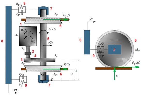
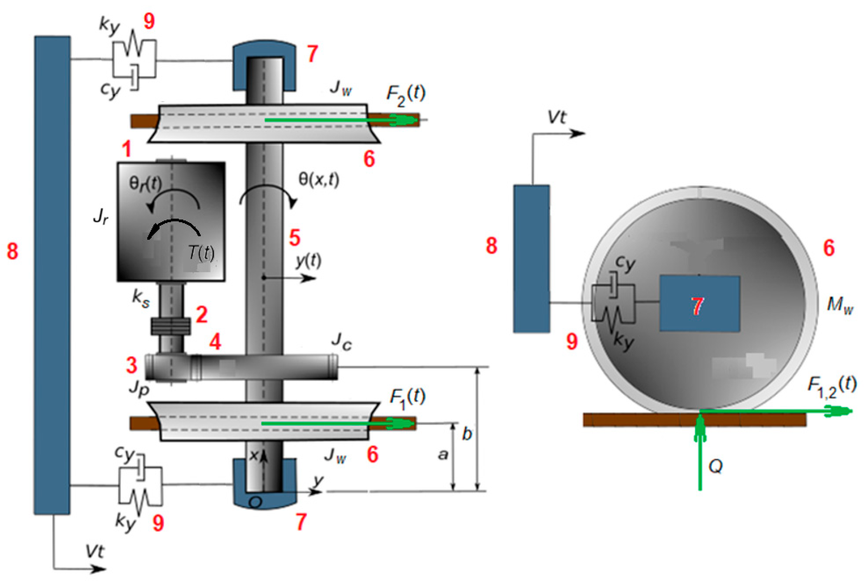
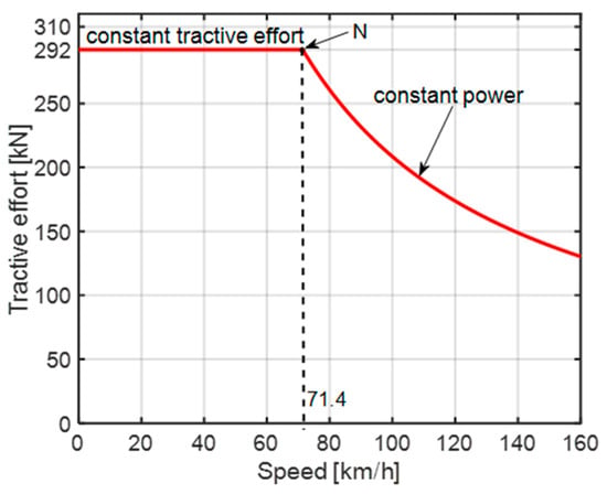
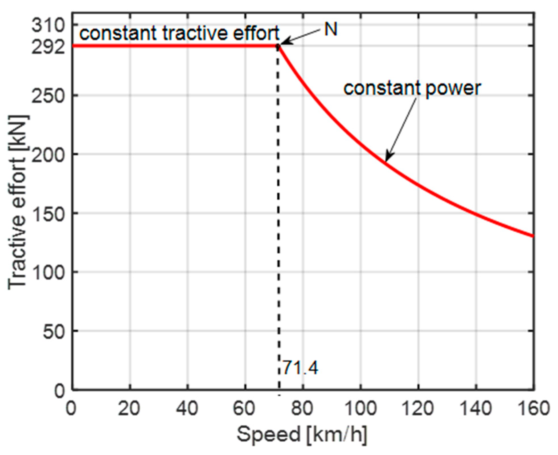
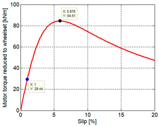
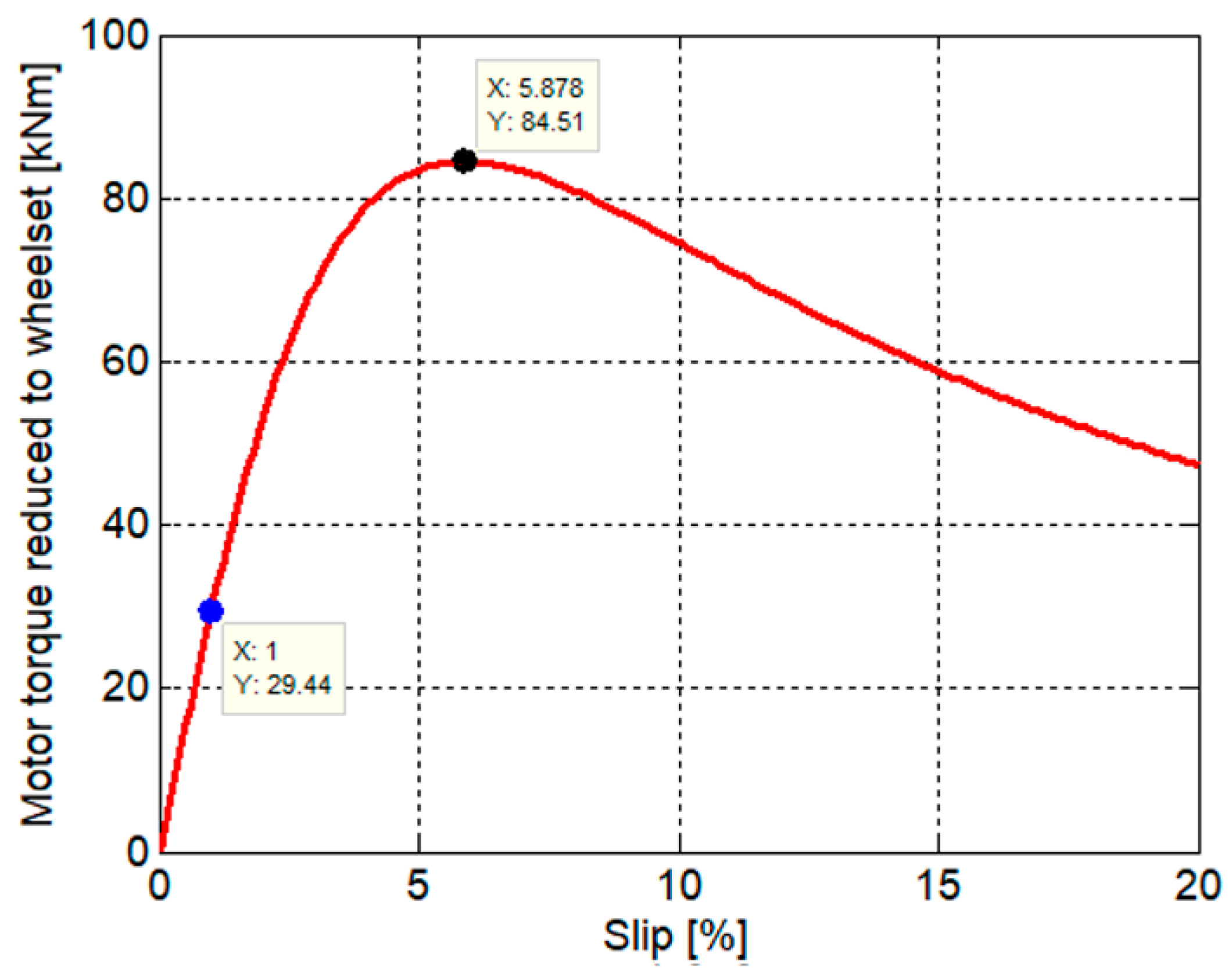
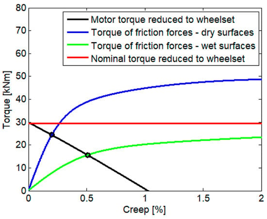
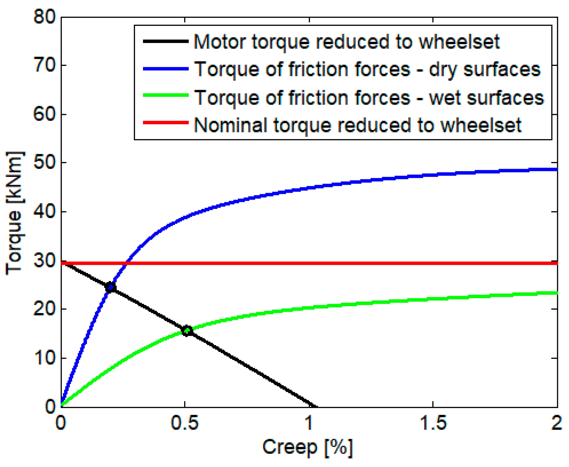
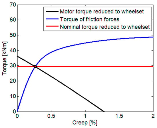
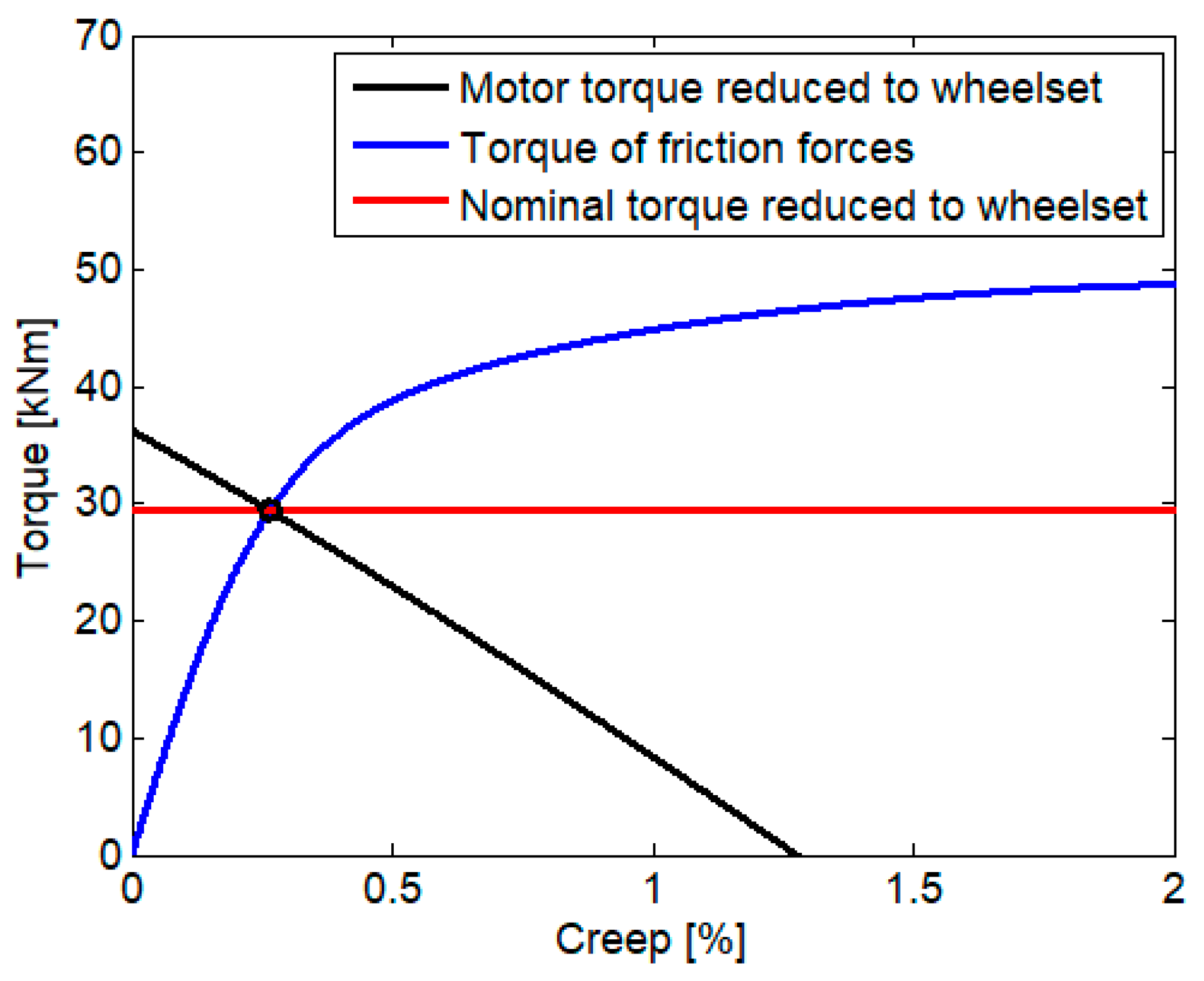
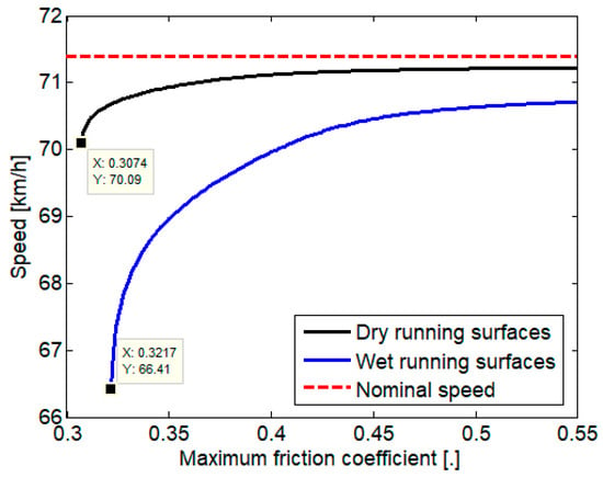
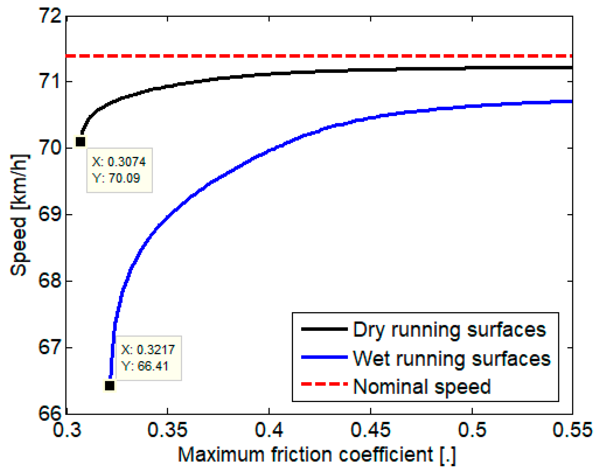
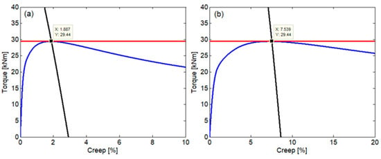
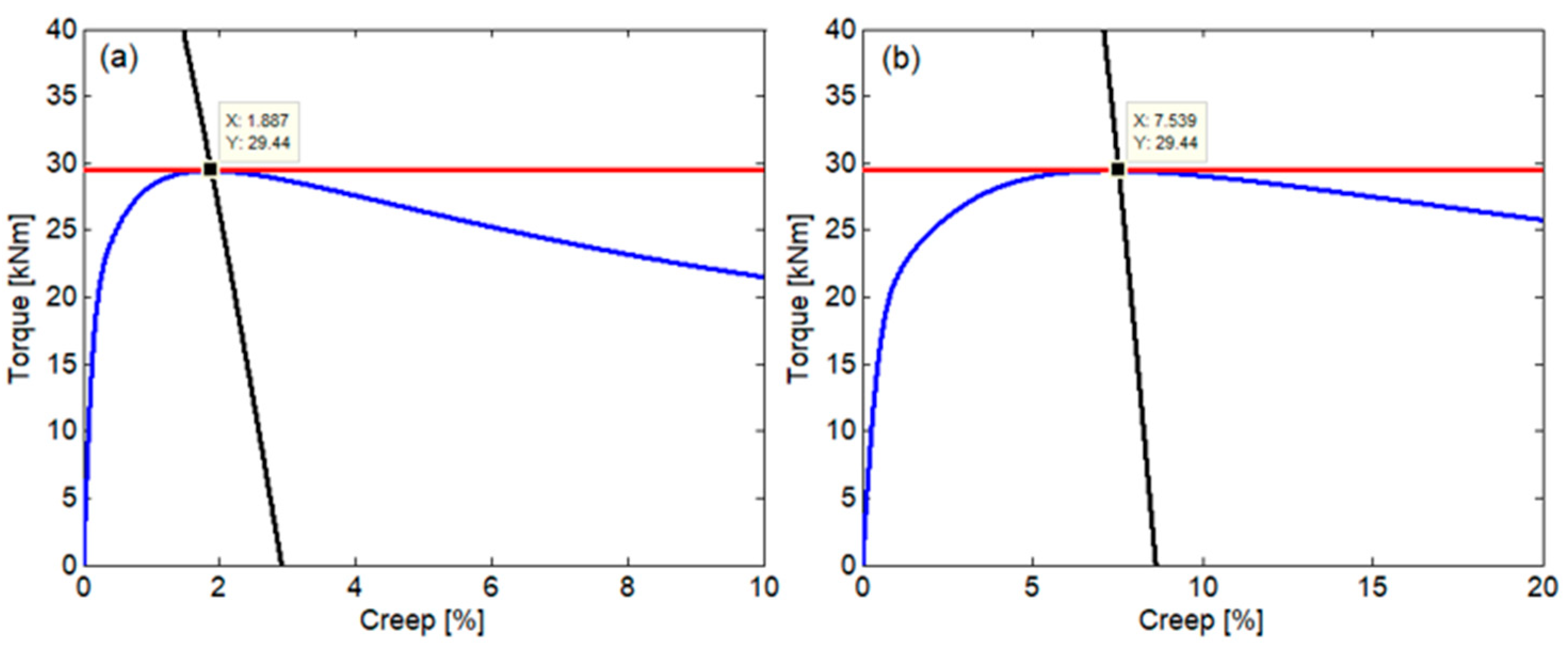
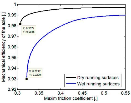
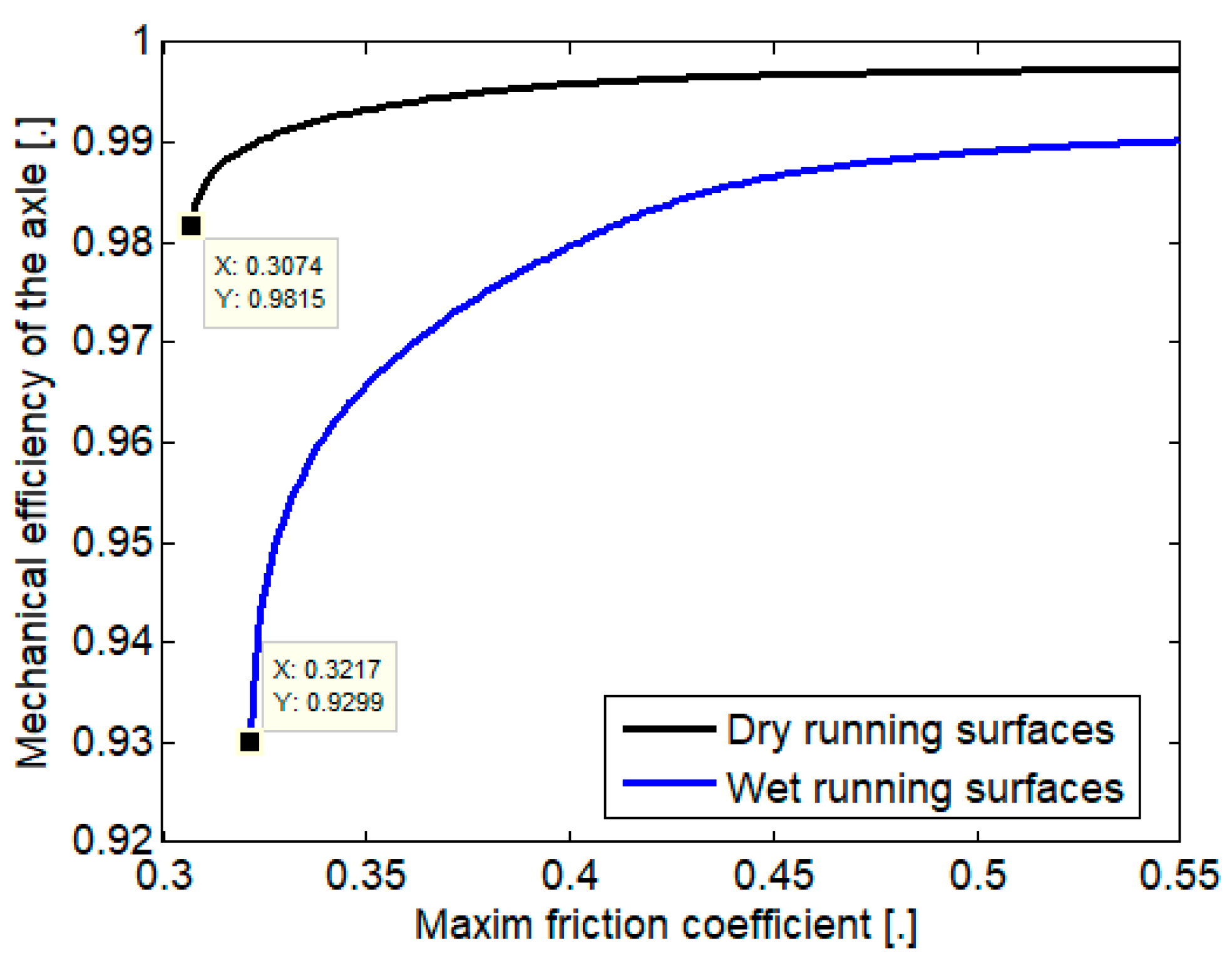
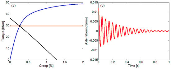
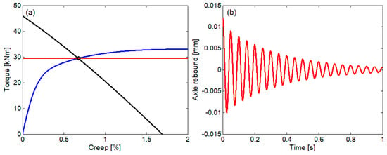
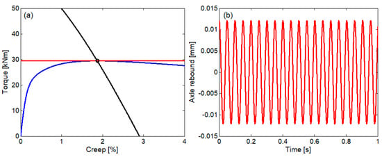
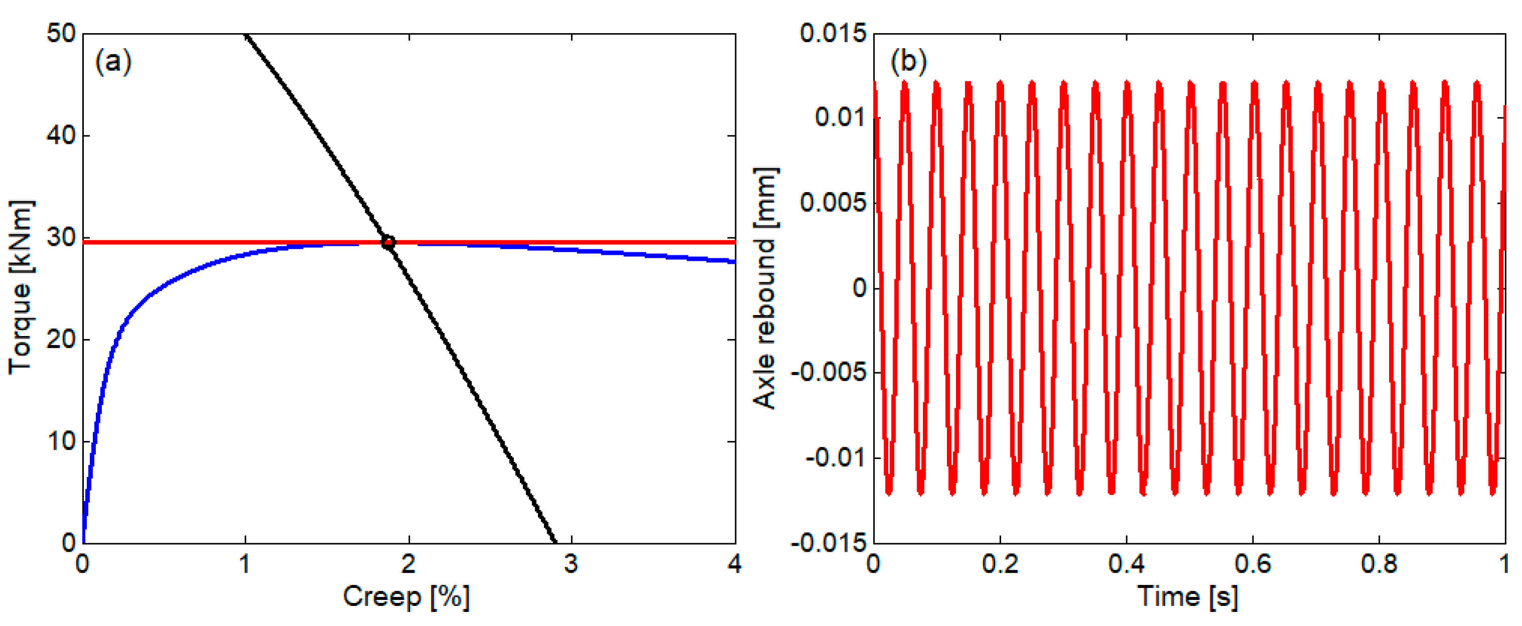
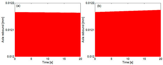
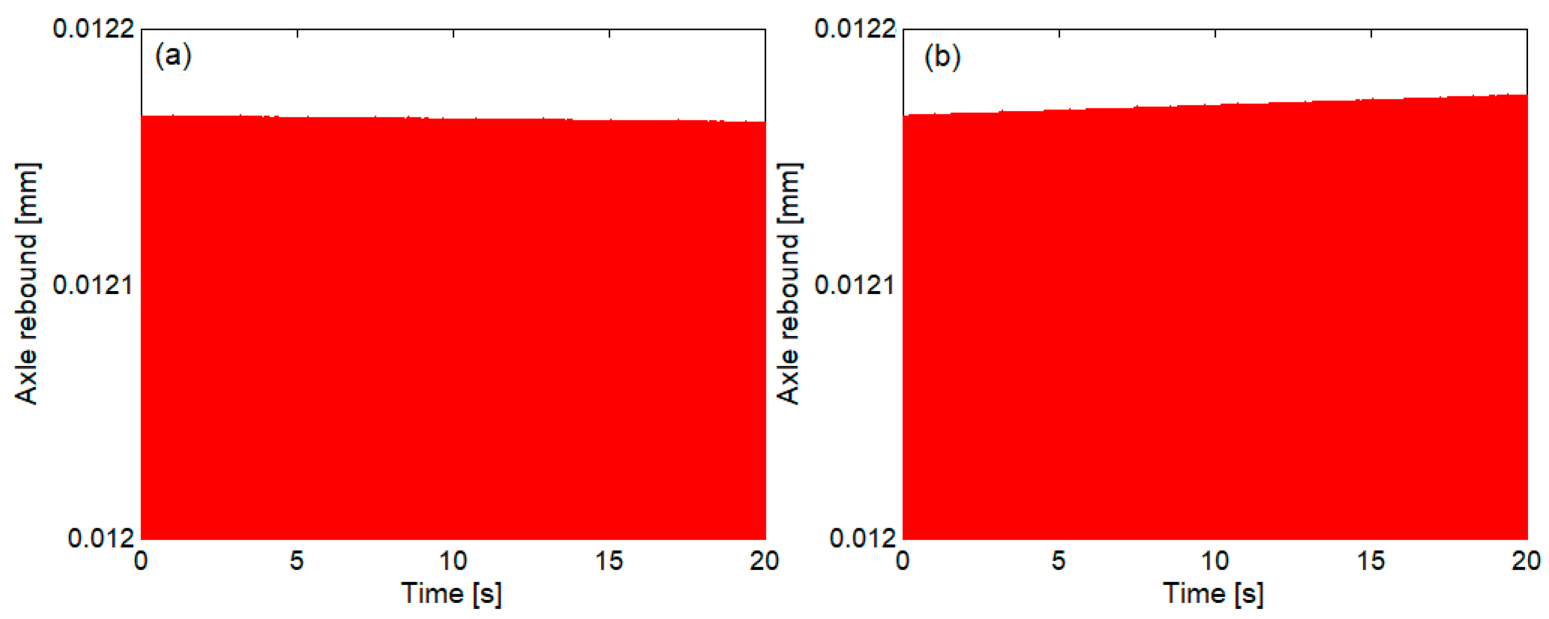
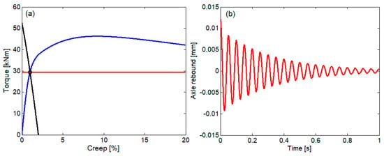
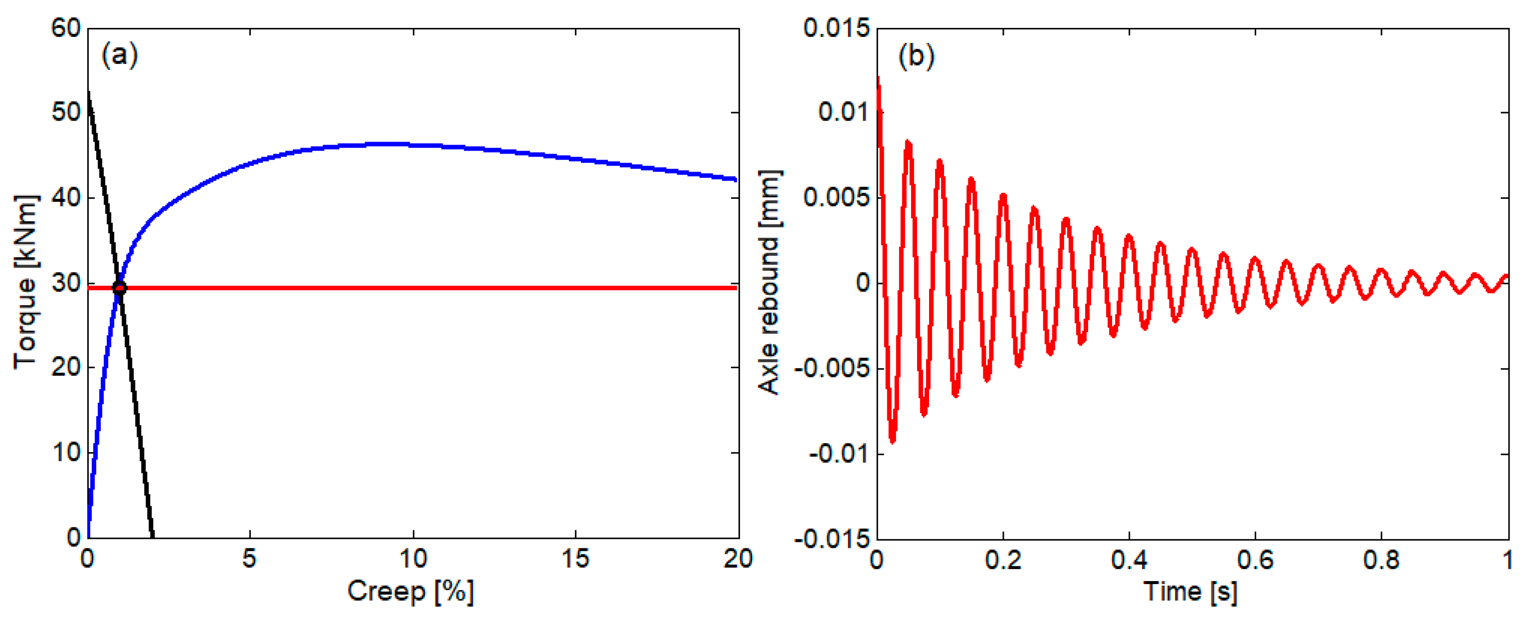
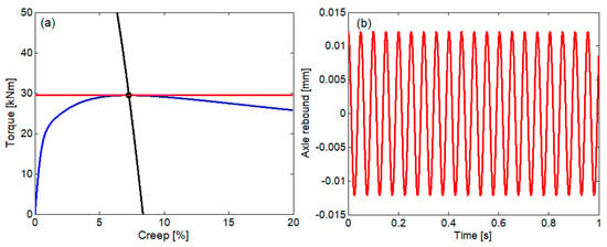
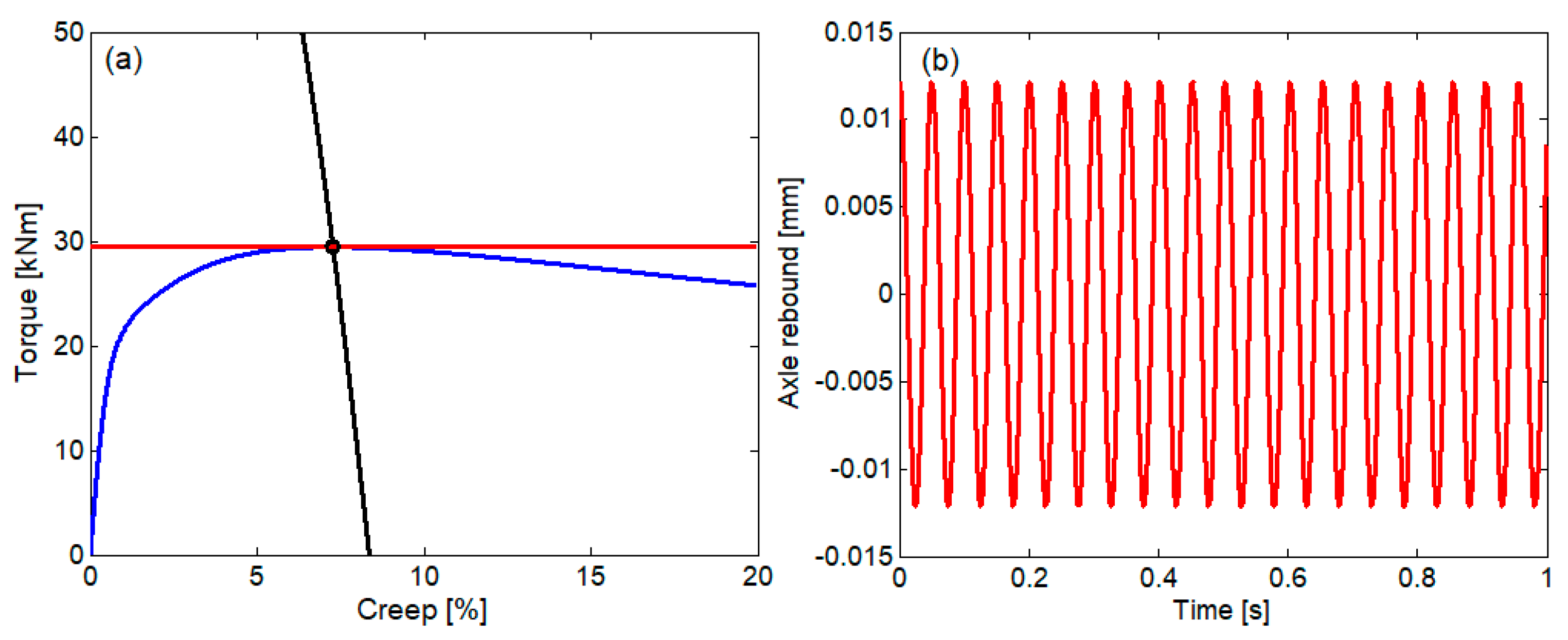
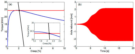
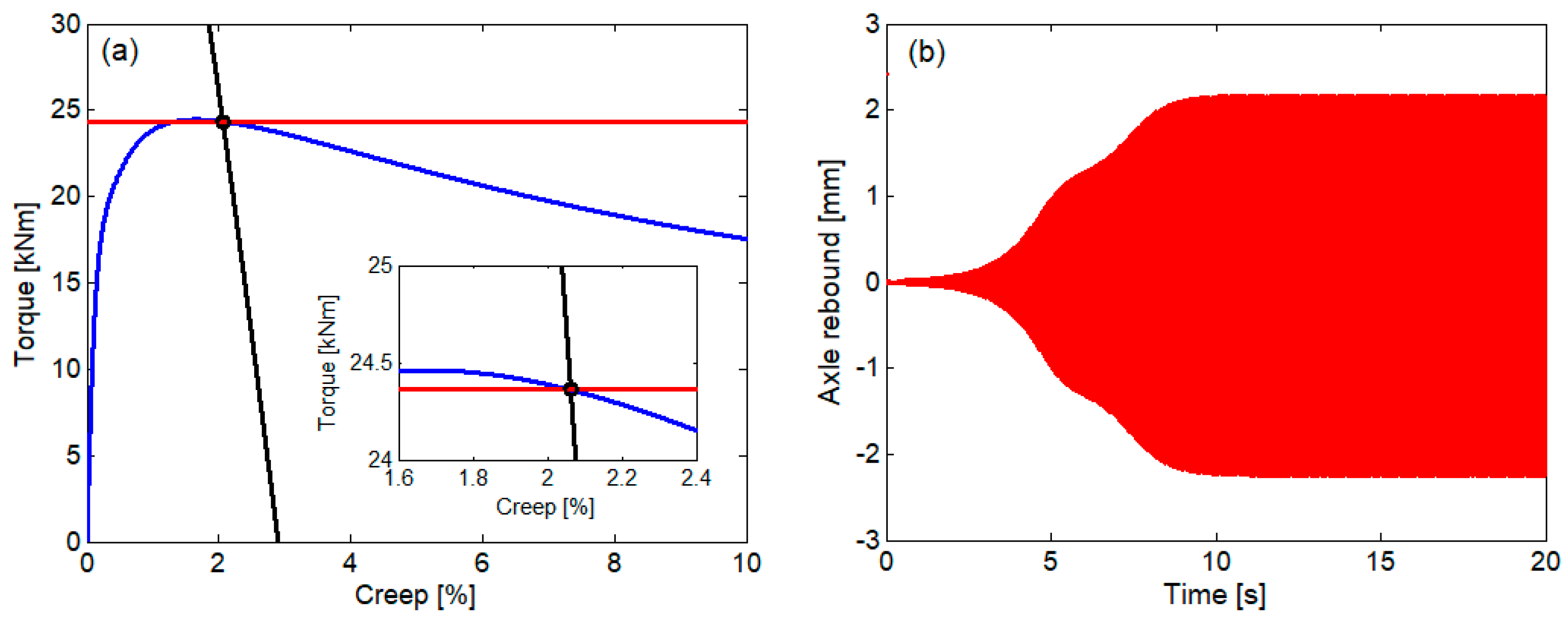
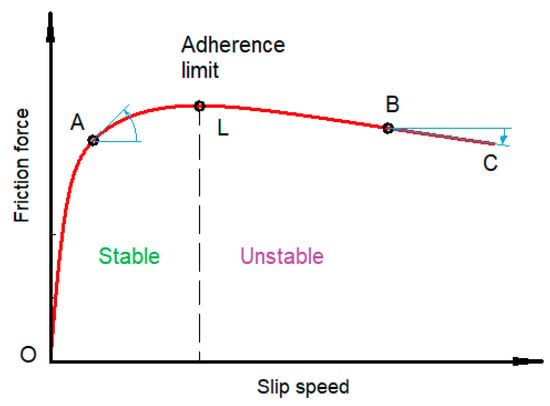
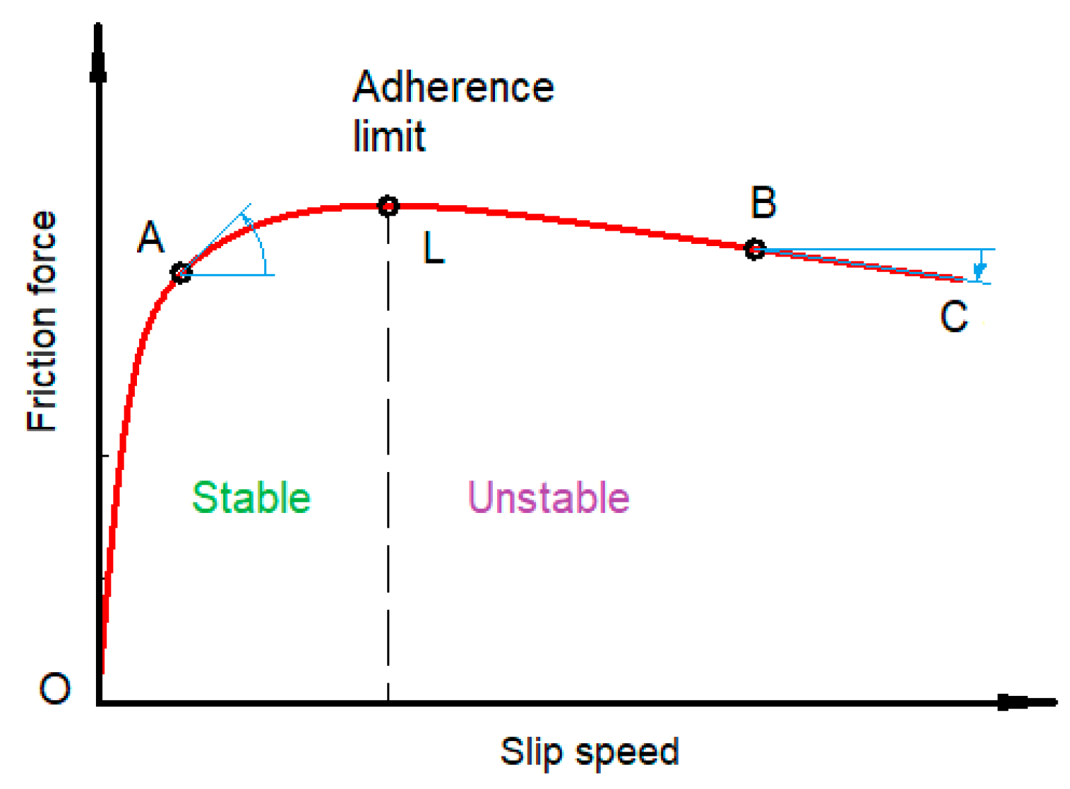
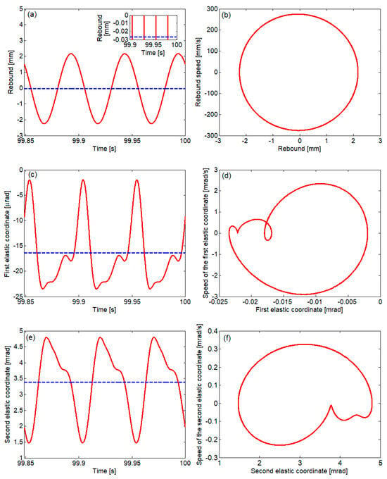
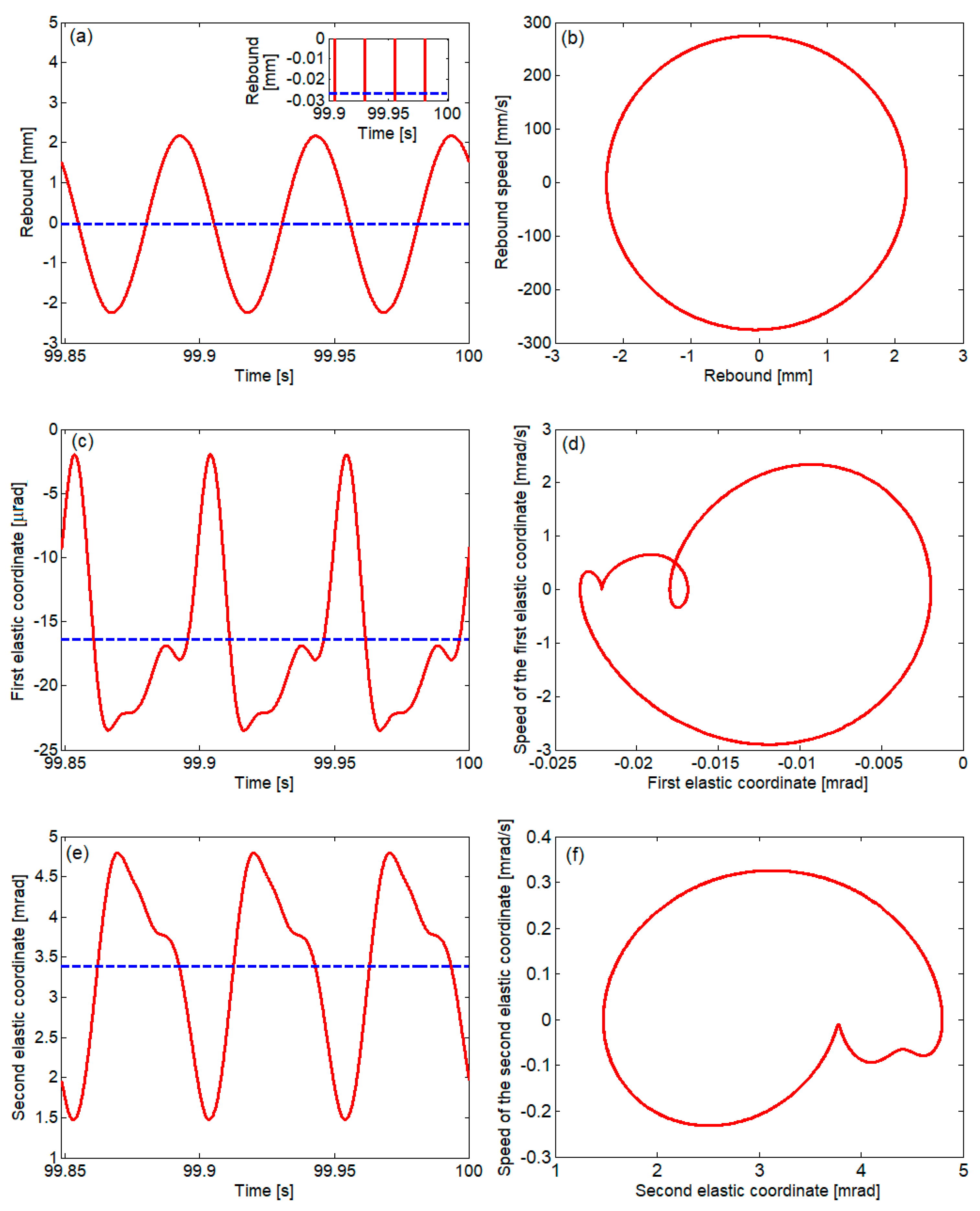
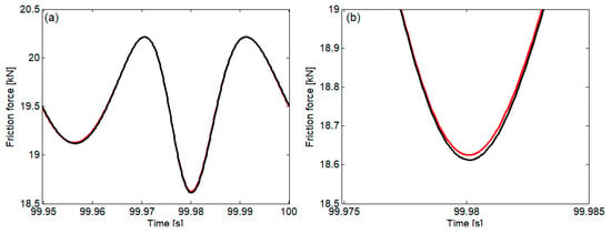
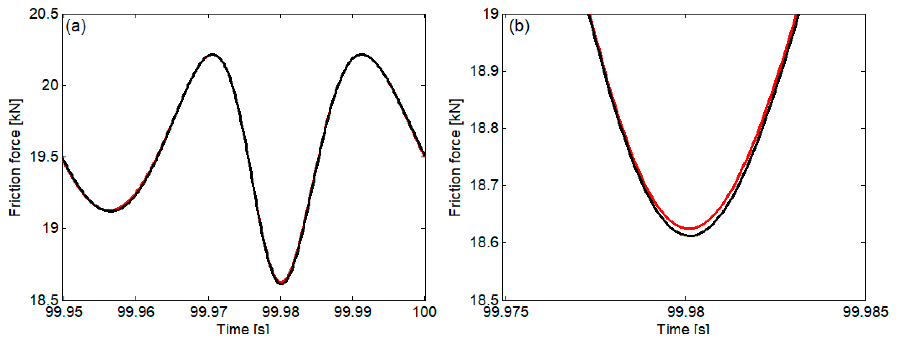
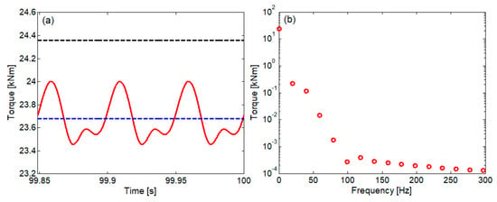
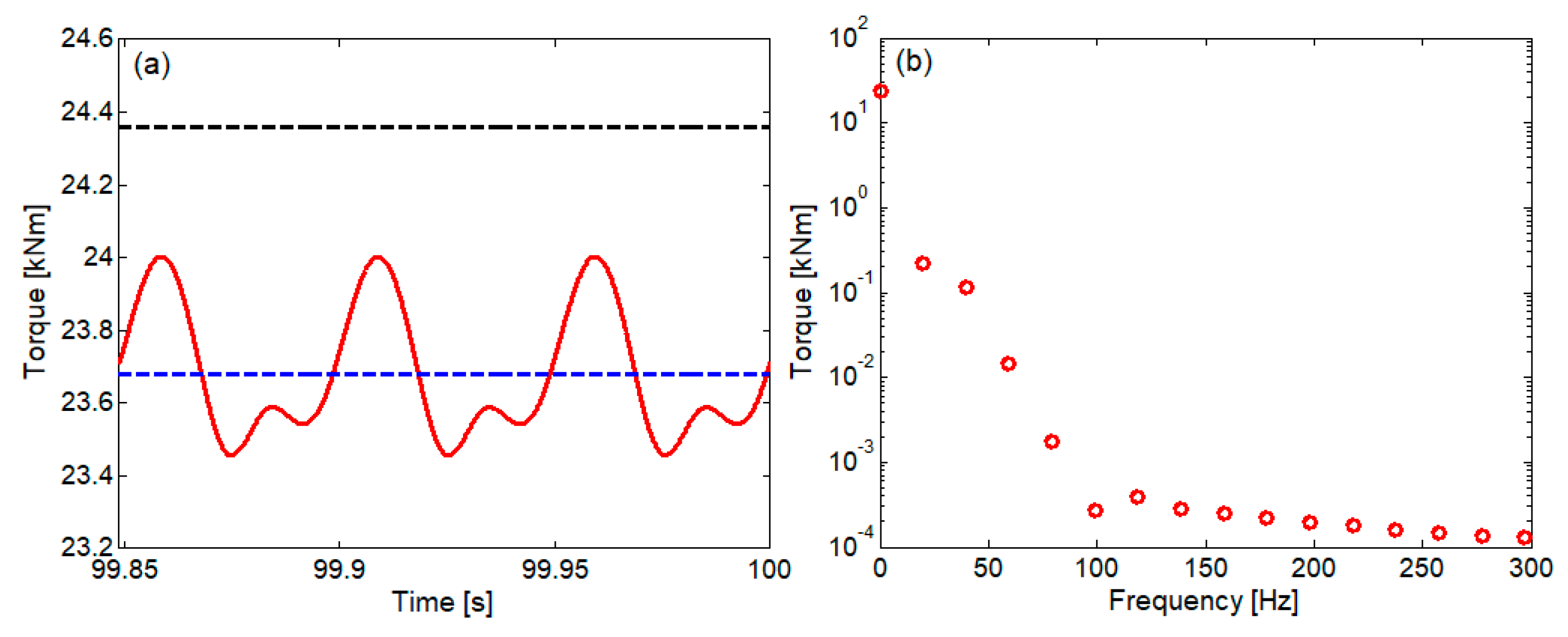
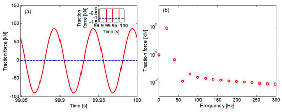
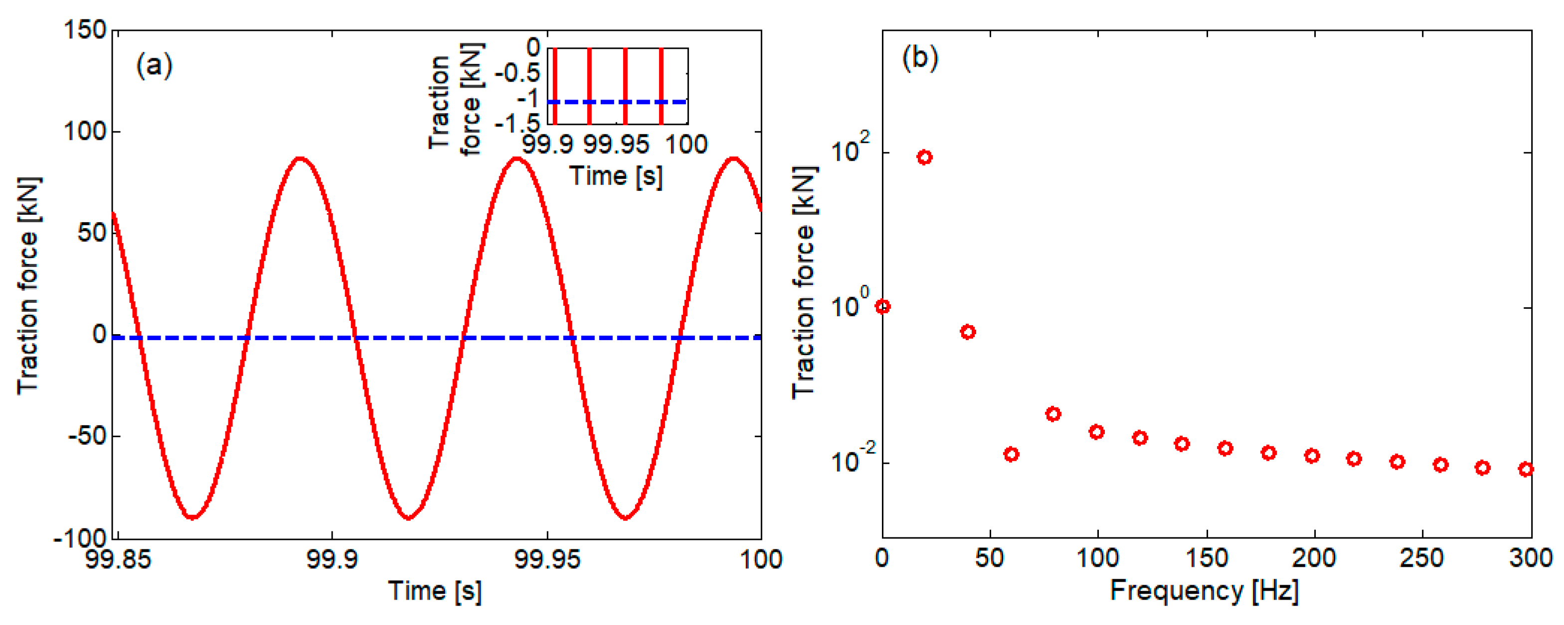
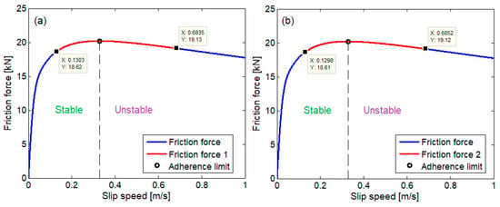
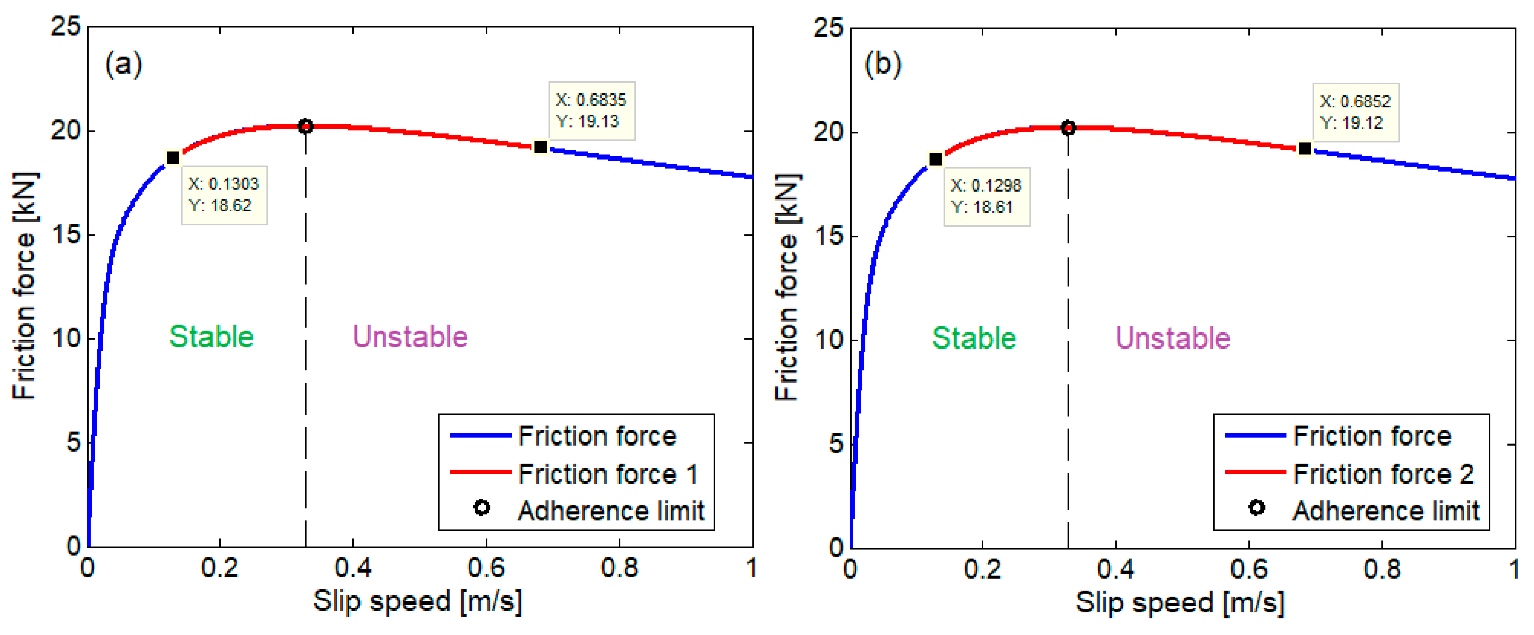
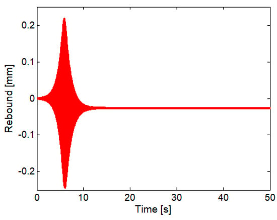
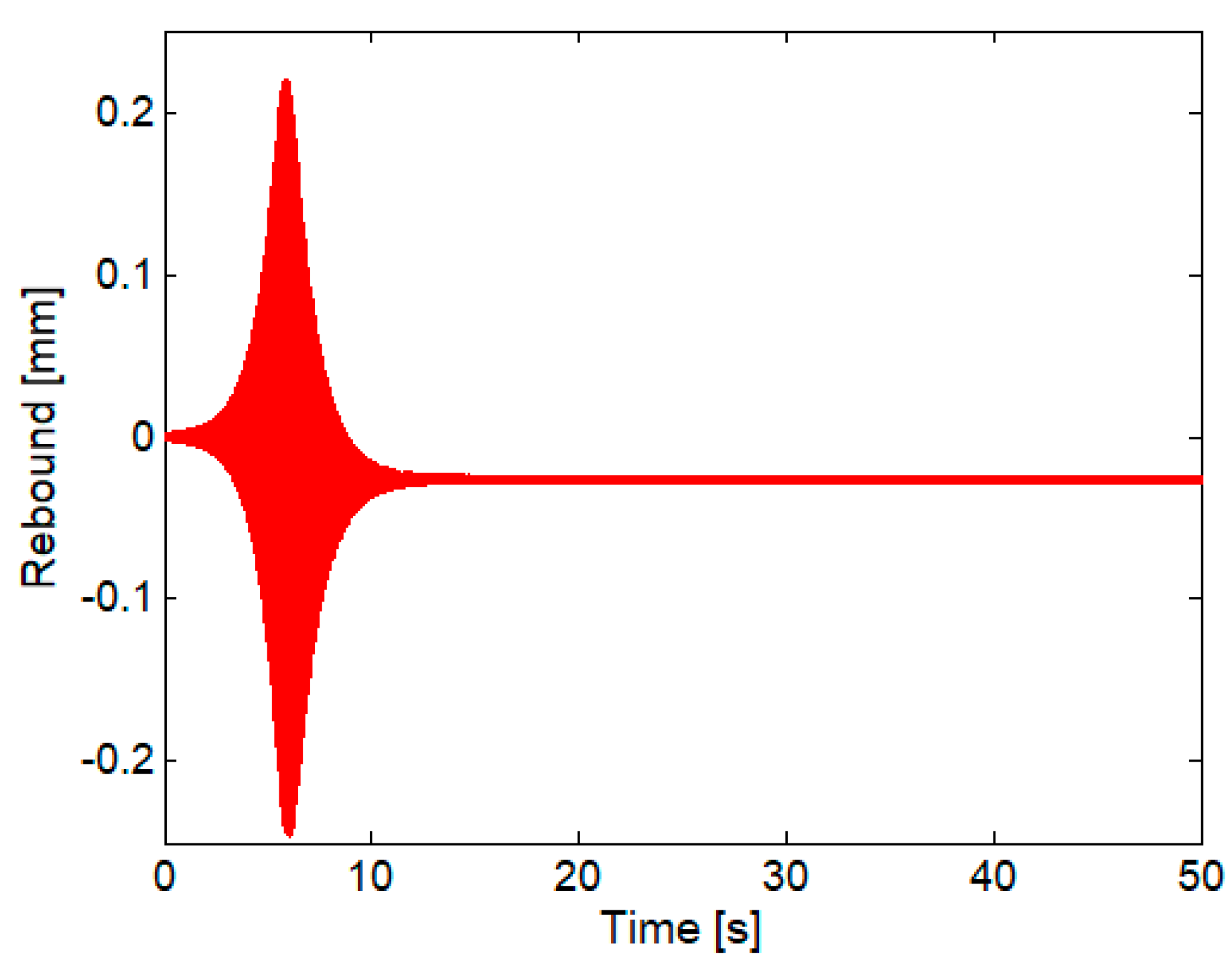
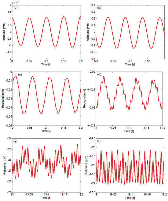
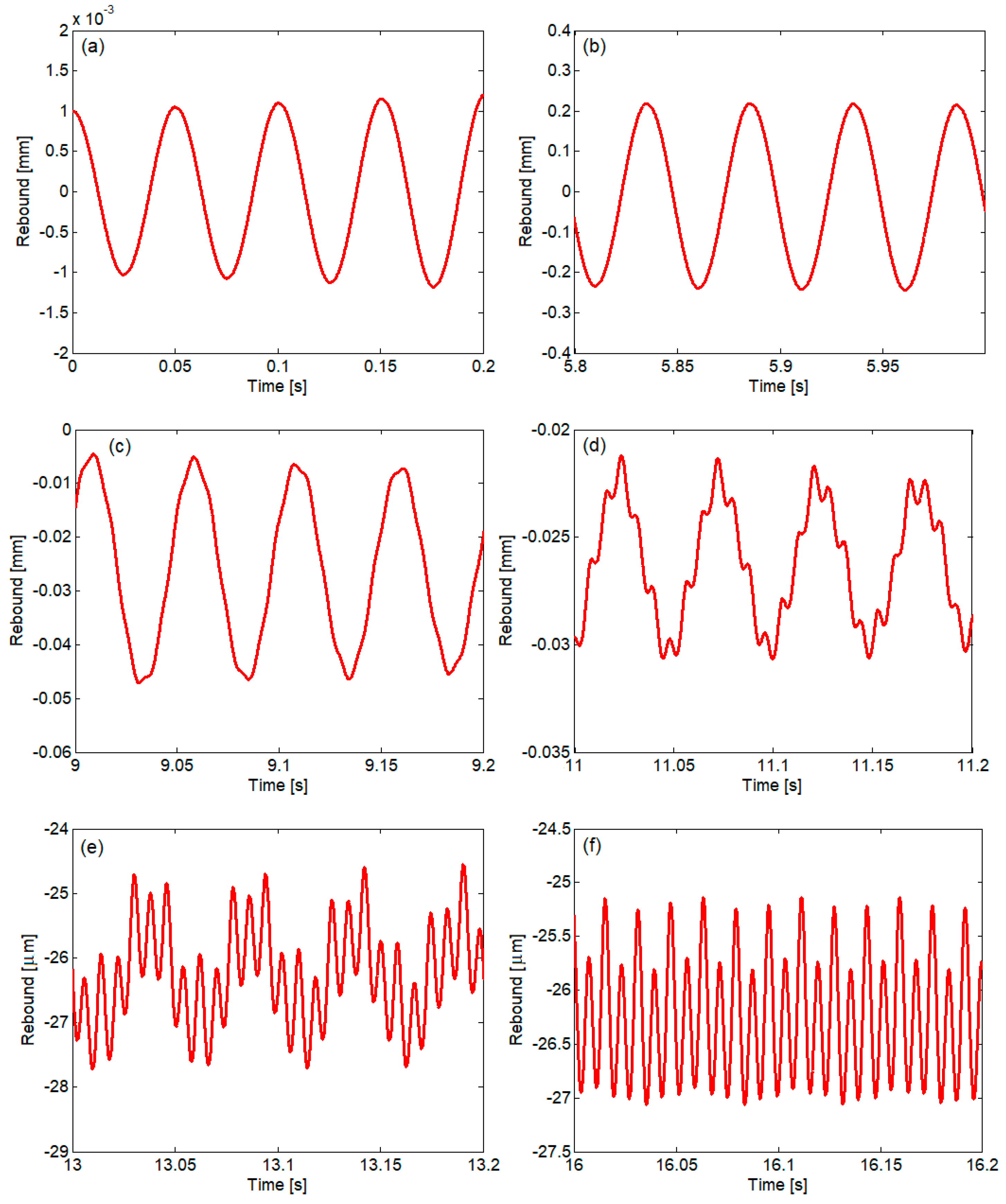
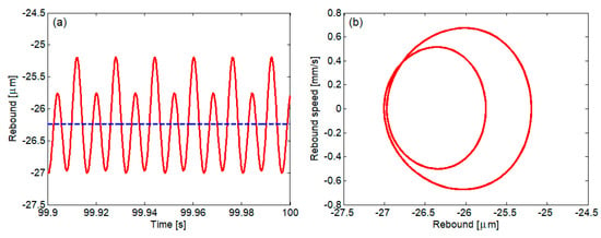
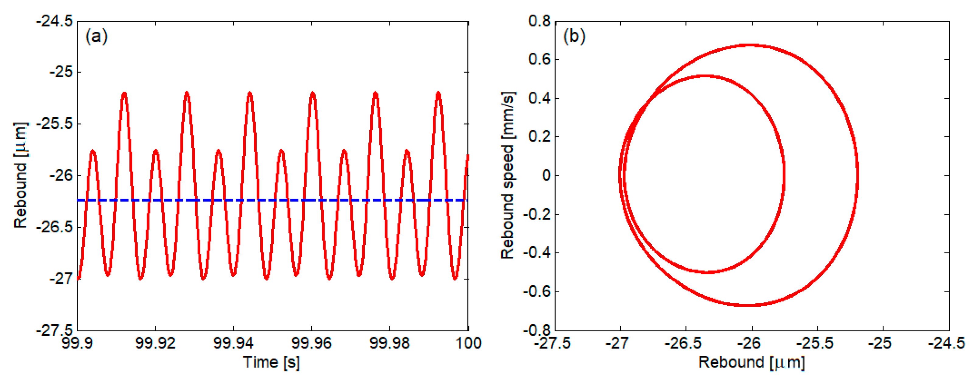
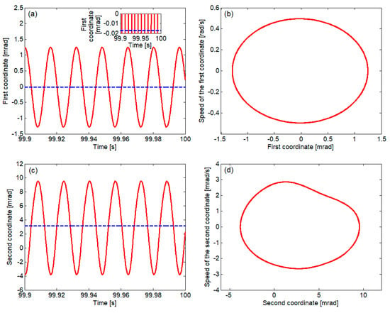
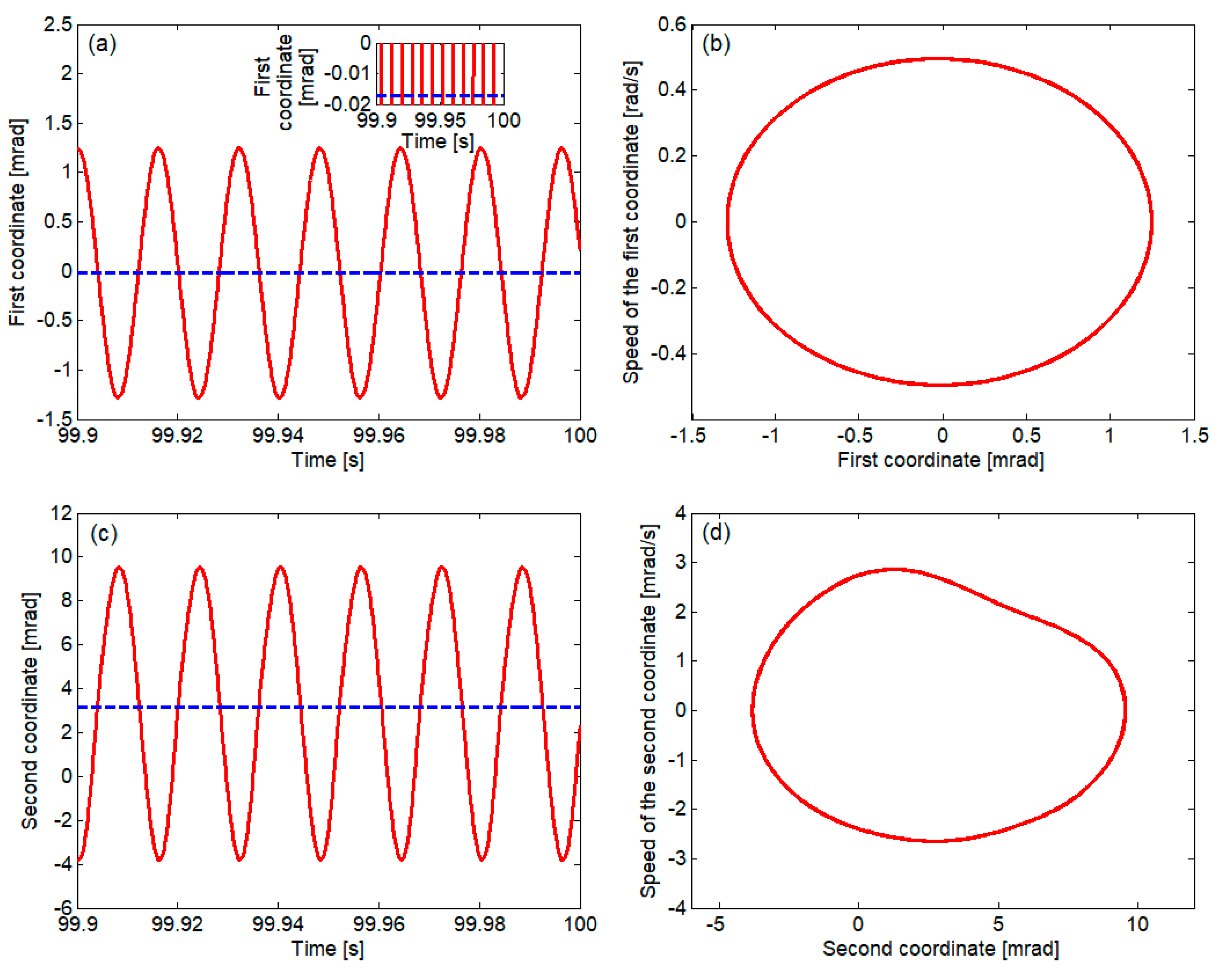
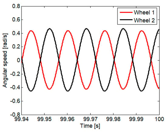
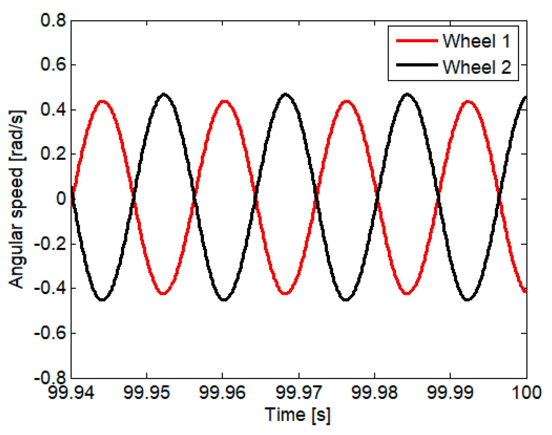
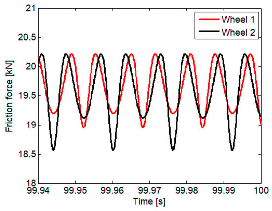
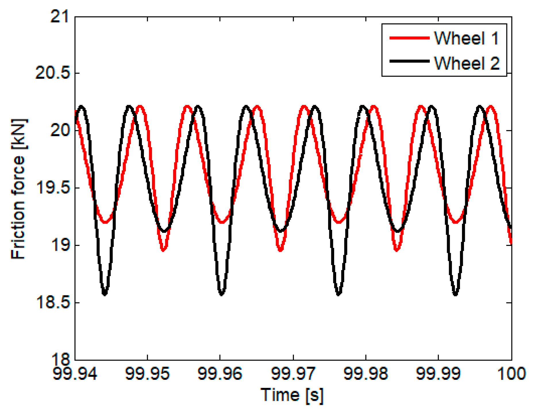
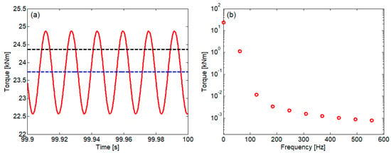
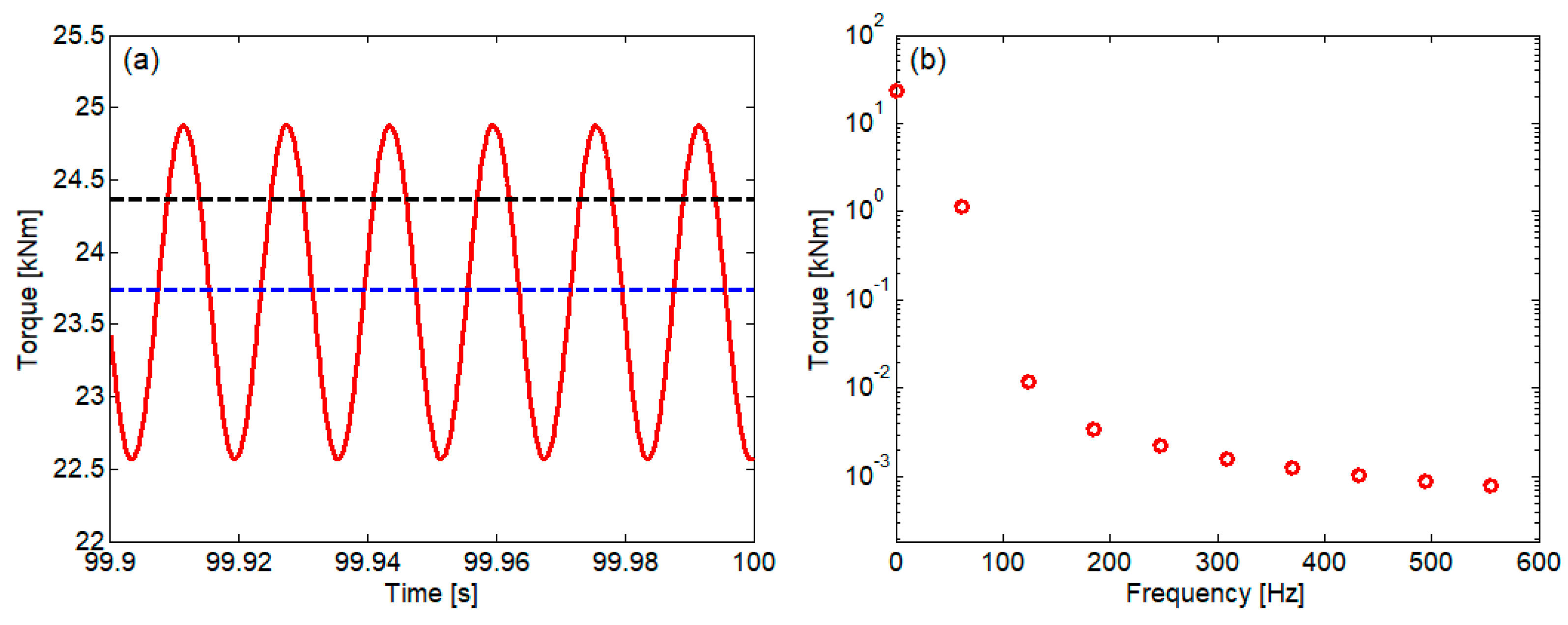
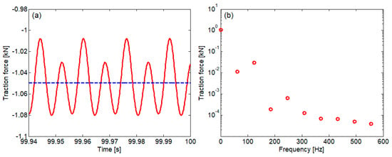
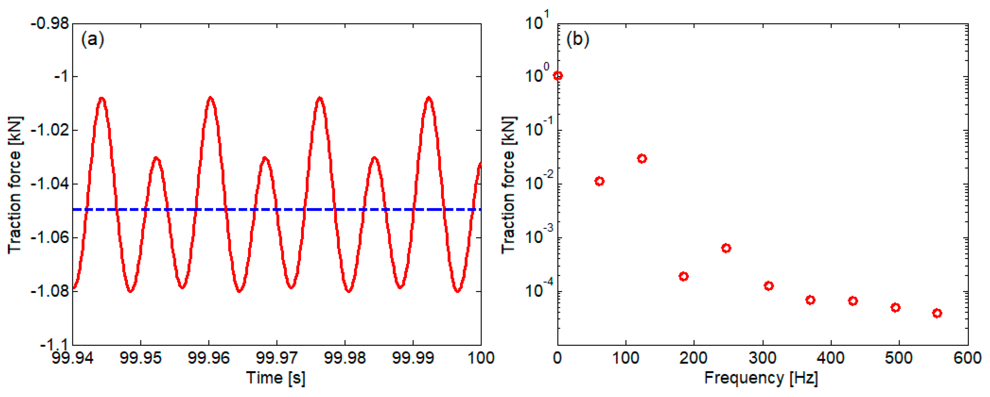
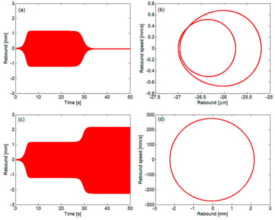
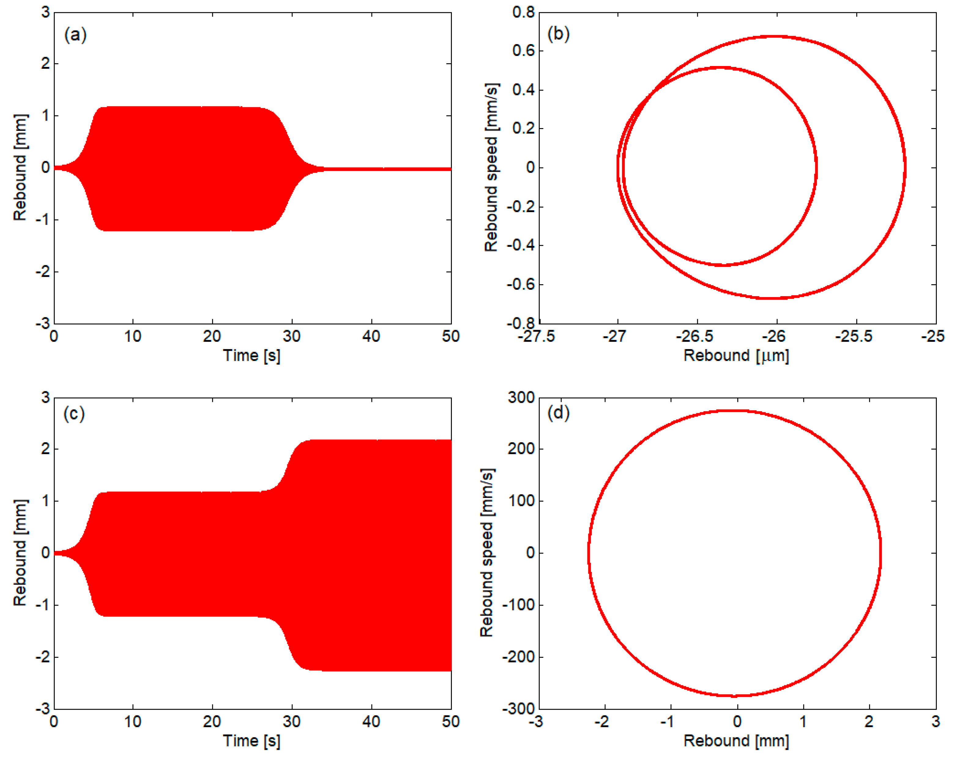
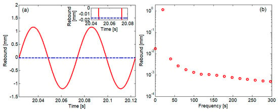
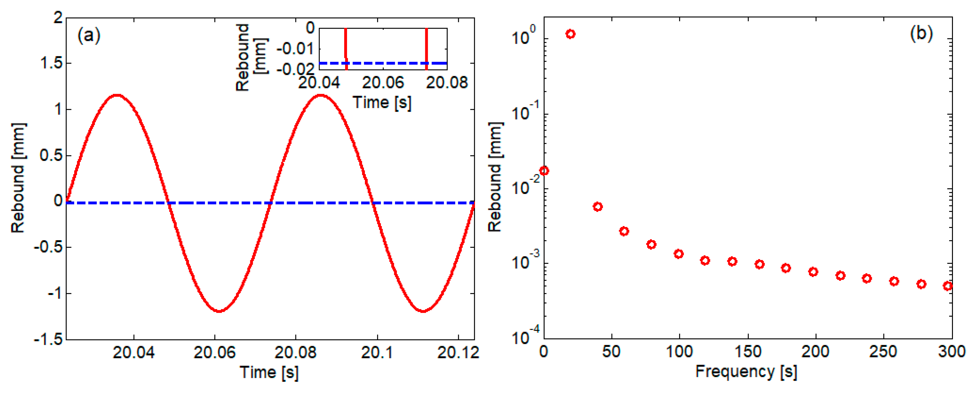
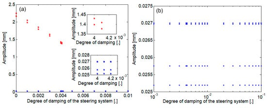
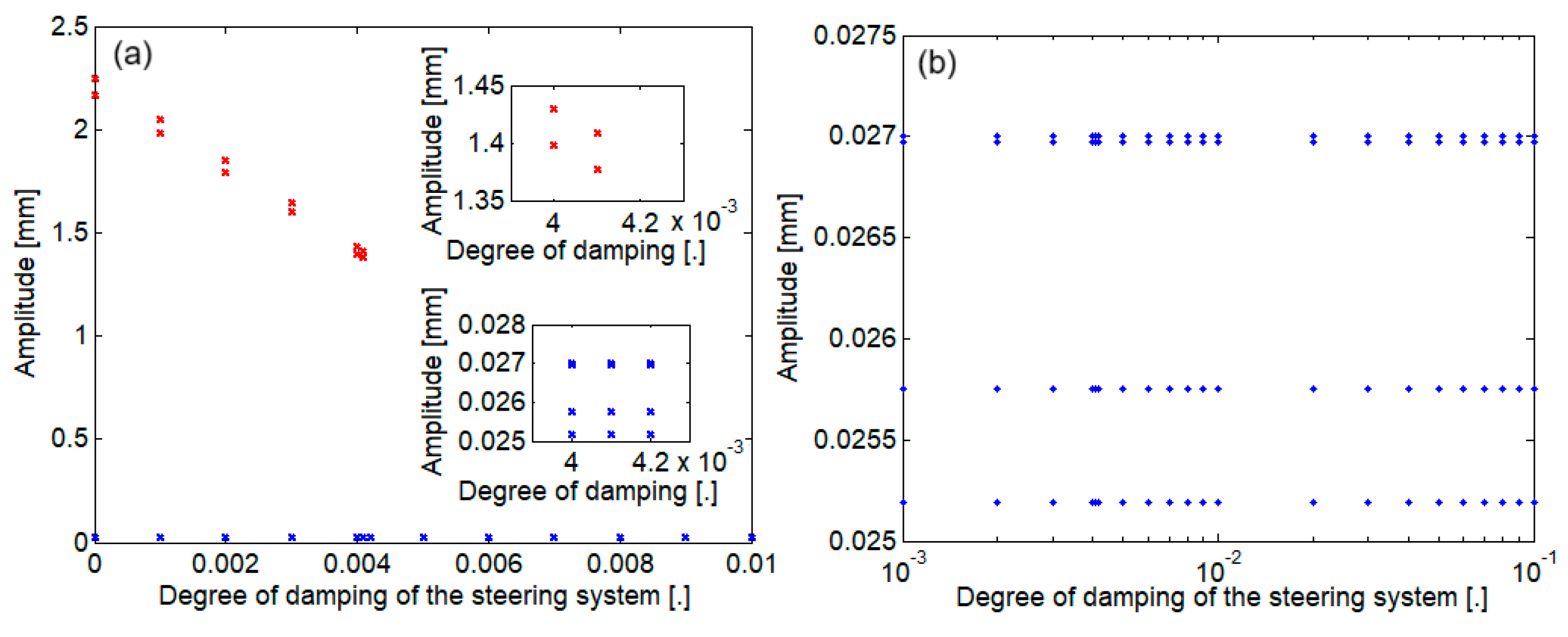
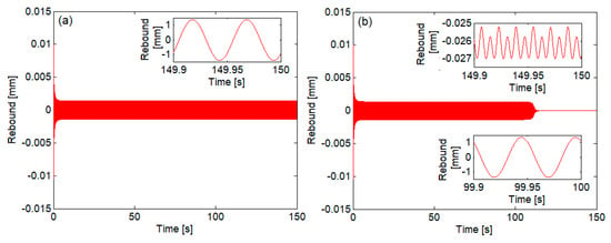
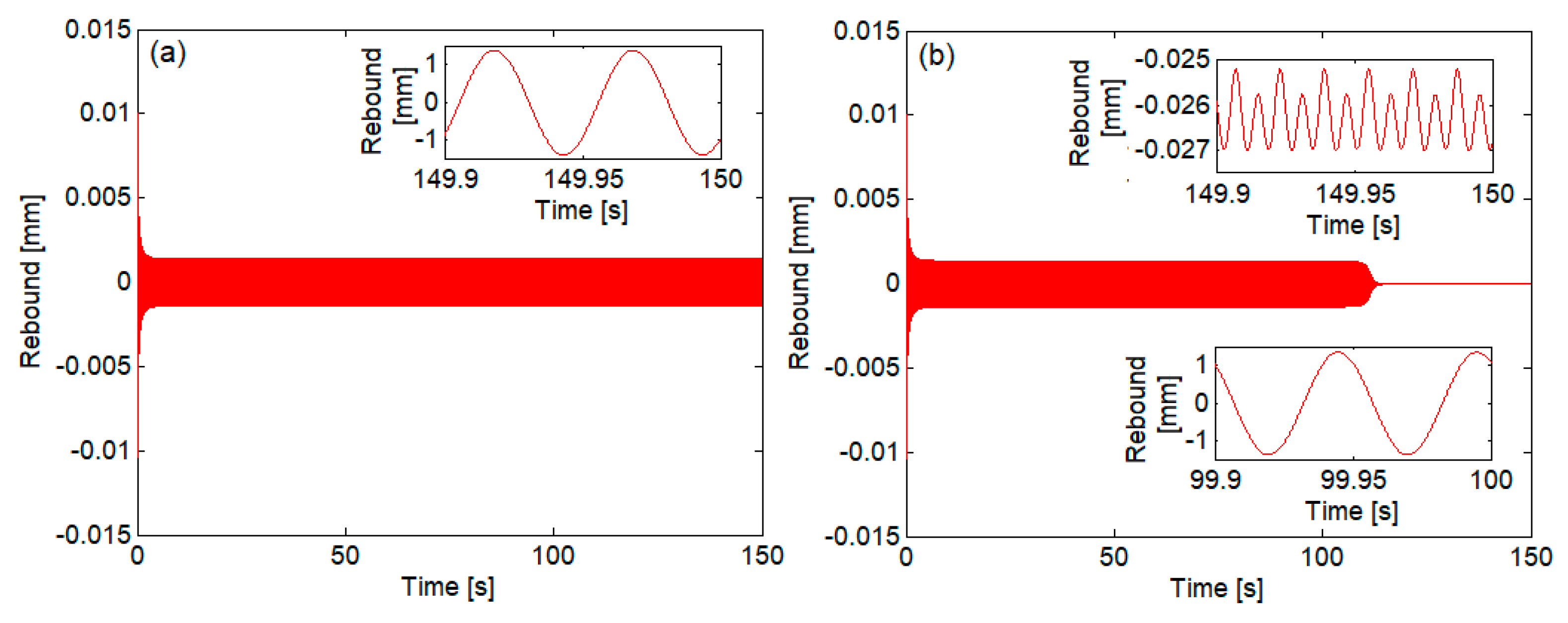
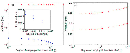
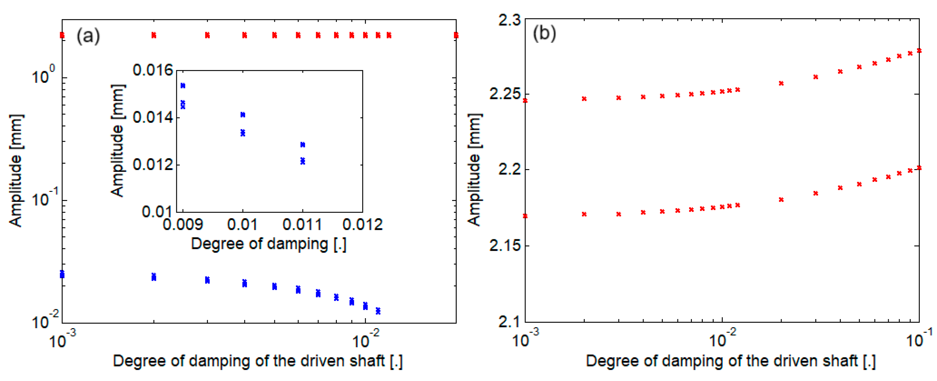
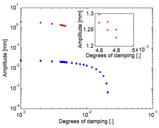
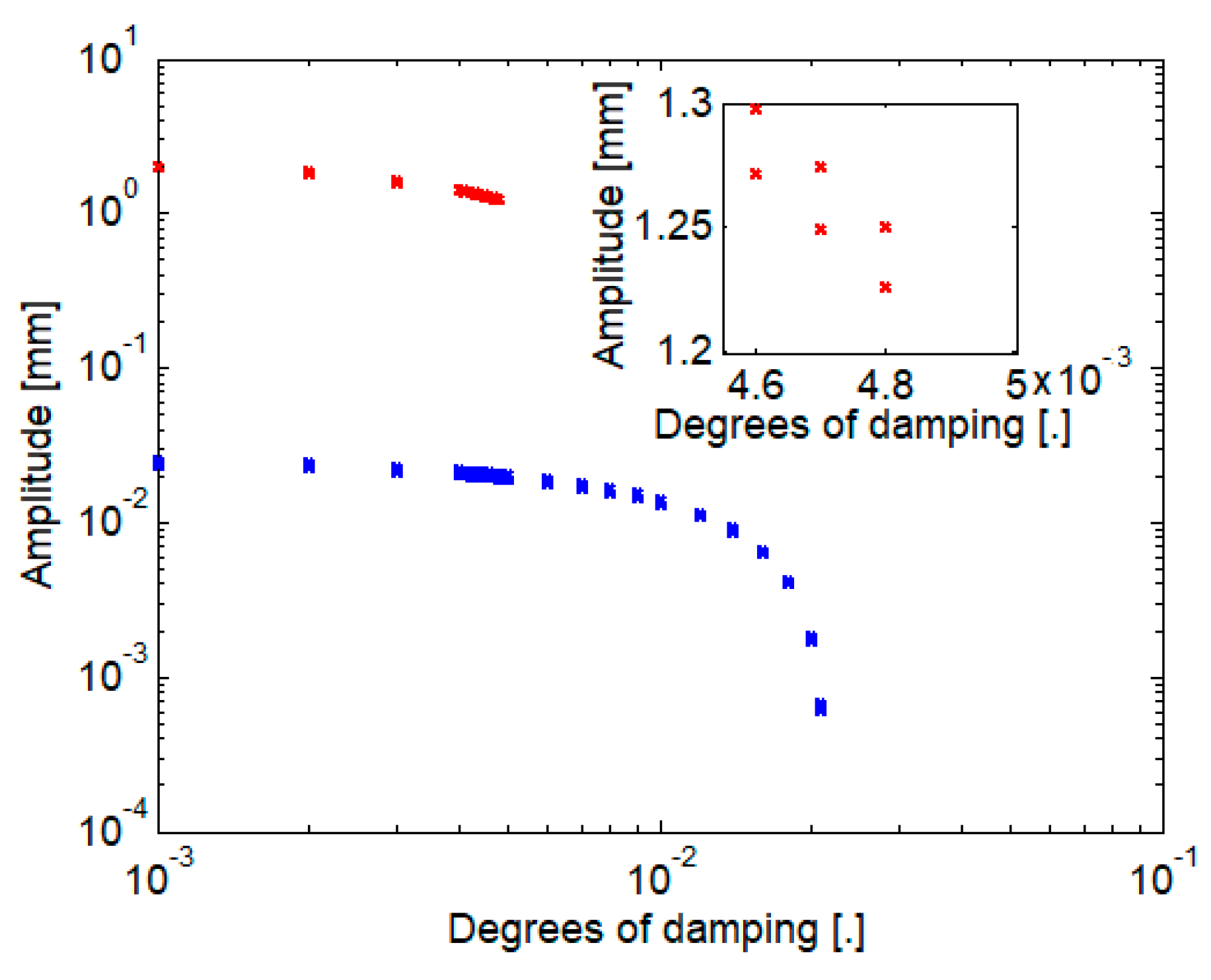

Disclaimer/Publisher’s Note: The statements, opinions and data contained in all publications are solely those of the individual author(s) and contributor(s) and not of MDPI and/or the editor(s). MDPI and/or the editor(s) disclaim responsibility for any injury to people or property resulting from any ideas, methods, instructions or products referred to in the content. |
© 2026 by the authors. Licensee MDPI, Basel, Switzerland. This article is an open access article distributed under the terms and conditions of the Creative Commons Attribution (CC BY) license.