


Abstract
Electrical-signature methods offer a non-invasive basis for induction-motor condition monitoring, but multimodal fusion does not necessarily improve prognosis when modalities have unequal reliability. This simulation-based study combines Motor Current Signature Analysis (MCSA), Instantaneous Power Signature Analysis (IPSA), reliability-weighted fusion, an interpretable health indicator, low-data Remaining Useful Life (RUL) estimation, measurement-noise analysis, and computational timing. A verified phase-coordinate induction-motor model was evaluated for healthy operation, progressive stator asymmetry, and reduced-circuit broken-rotor-bar (BRB) cases. For stator asymmetry, the reliability-weighted health trajectory was strictly directional in all 72 evaluated states. Reliability weighting improved over equal fusion and IPSA-only prognosis but did not outperform MCSA-only RUL accuracy. Across all diagnostic inputs, a free-intercept linear model outperformed the exponential model; MCSA-LIN achieved the lowest clean normalized-RUL MAE and RMSE of 0.082690 and 0.084853, respectively. Under synthetic electrical noise, p05–p95 intervals contained the clean estimate in all 360 cells but the synthetic truth in none, showing that measurement-noise dispersion was much smaller than deterministic bias. For BRB diagnosis, slip-tracked current sidebands were primary and low-frequency power signatures were complementary. The worst complete stator-diagnostic p95 latency was 6.350665 ms for a 2 s acquisition window. These results provide a reproducible simulation-only baseline for subsequent experimental validation.
1. Introduction
Induction motors (IMs) remain central to industrial electromechanical systems because of their rugged construction, favorable cost-to-power ratio, and widespread use in manufacturing, transportation, pumping, ventilation, compression, and other continuously operated assets [1,2,3,4]. Despite this robustness, electrical, rotor, stator, bearing, and other electromechanical faults can evolve under service conditions and may lead to unplanned downtime, secondary damage, and maintenance costs. Recent experimental and modeling studies continue to address induction-motor behavior and fault detection across steady and transient operating conditions, illustrating the importance of accounting for load, speed, supply condition, and operating regime when interpreting diagnostic signals [3,4]. Consequently, induction-motor condition monitoring has developed beyond protection-oriented fault detection toward health assessment, predictive maintenance, and prognostic applications.
Among non-invasive approaches, electrical signature analysis is attractive because stator voltages and currents are often already measurable at the supply or drive interface. Motor Current Signature Analysis (MCSA) relates fault-induced modulation to characteristic components of the stator-current spectrum and has a long history in induction-motor diagnosis [5,6,7]. Broader diagnostic reviews also show that electrical signatures coexist with vibration, flux, thermal, acoustic, and other modalities, each with different sensitivities and instrumentation requirements [2,8]. Instantaneous-power-based analysis extends the electrical view by combining voltage and current information; seminal and comparative studies showed that power spectra can reveal fault-related components that are weak, shifted, or represented differently in the current spectrum [9,10]. Earlier work by Zagirnyak, Mamchur, and Kalinov developed and experimentally examined the joint use of current and instantaneous-power spectra for induction-motor diagnosis, including comparison of their informative value under stator and rotor faults [11,12].
Diagnosis, however, is not equivalent to prognosis. A diagnostic feature can be sensitive to a fault yet still be unsuitable as a degradation coordinate if it is non-monotonic, strongly load-dependent, poorly normalized, or unstable under measurement noise. Prognostics and Health Management (PHM) research for induction machines therefore extends beyond fault detection to health assessment, degradation representation, and Remaining Useful Life (RUL) prediction [13]. One induction-motor study demonstrated the use of a constructed health index (HI) with nonlinear degradation modeling and experimental run-to-failure data, illustrating the value of explicitly linking HI geometry to the selected RUL model [14]. In the broader rotating-machinery literature, multi-domain feature fusion and HI construction have been used to improve monotonicity, robustness, and degradation representation [15,16].
This transition introduces two additional methodological issues. First, the present study adopts the working premise that multimodal fusion should account for unequal diagnostic quality rather than assume that all modalities deserve equal influence. Recent motor-fusion research shows that heterogeneous current and electromagnetic measurements can provide complementary diagnostic information [17], while broader rotating-machinery research has investigated explicit sensor-reliability weighting when channel quality differs [18]. Recent induction-motor studies also illustrate the importance of simulation-to-experiment comparison [19] and experimentally anchored health monitoring in data-scarce settings [20]. These studies support reliability-aware evaluation, but they do not imply that fusion must outperform the strongest individual modality; that question is tested explicitly here. Second, RUL uncertainty must be interpreted according to the uncertainty sources actually propagated. Prognostic uncertainty can arise from measurements, model form, parameters, degradation variability, thresholds, operating conditions, and domain mismatch [21]. Recent evaluation frameworks distinguish point accuracy from uncertainty, robustness, interpretability, and computational feasibility [22], while dedicated reviews emphasize the need to state which uncertainty sources are represented by a reported interval [23]. Physics-informed data-driven prognosis offers a longer-term route for combining physical constraints with learned degradation representations, but such methods also depend on data quality, model fidelity, and generalization evidence [24].
Against this background, the present study addresses a deliberately narrower baseline question: how far can a transparent physics-guided electrical-signal pipeline be taken when physical run-to-failure data are not yet available? Rather than introducing a high-capacity learning model, the study combines a verified induction-motor simulator, requested-frequency MCSA and Instantaneous Power Signature Analysis (IPSA), reliability-weighted feature fusion, an interpretable bounded HI, two low-data parametric RUL models, electrical measurement-noise propagation, explicit ablations, and computational timing. The simulation-only design is intentional. It provides a controlled environment in which diagnostic sensitivity, load dependence, fusion behavior, model-form bias, and noise-induced dispersion can be separated before experimental validation is attempted.
The novelty of the present work lies in the integrated, reproducible evaluation framework and the evidence it generates, rather than in proposing a new MCSA algorithm, IPSA algorithm, fusion operator, or RUL estimator. The paper contributes the following:
- (i)
- a verified physics-guided evaluation baseline spanning healthy operation, progressive stator asymmetry, and reduced-circuit broken-rotor-bar (BRB) cases;
- (ii)
- a controlled modality and fusion ablation using requested-frequency MCSA and IPSA features with reliability weights calibrated from diagnostic behavior rather than from RUL outcomes;
- (iii)
- an interpretable progressive stator HI and a matched low-data prognosis benchmark comparing exponential and free-intercept linear models under identical causal prefixes, including forecast-origin and endpoint-sensitivity analysis;
- (iv)
- source-specific uncertainty and deployment evaluation that separates AWGN-induced dispersion, load/model-form/endpoint/slip-locator sensitivity, deterministic prediction bias, and in-memory computational feasibility.
Four research questions organize the evaluation.
RQ1 asks whether the physics-guided MCSA and IPSA features provide directional, load-robust diagnostic evidence and whether reliability weighting improves on equal fusion when the modalities have unequal quality.
RQ2 asks which of the four diagnostic inputs provides the strongest low-data normalized-RUL baseline and whether the exponential degradation model is actually preferable to a linear alternative.
RQ3 asks how electrical measurement noise contributes to RUL dispersion relative to deterministic prediction error.
RQ4 asks whether the complete diagnostic and low-data RUL calculations are computationally lightweight relative to the fixed acquisition window on the tested workstation.
These questions are answered only for the predefined simulation protocol and are not presented as experimental or field validation.
The remainder of the paper is organized as follows. Section 2 positions the study relative to electrical-signal diagnosis, physics-based fault modeling, feature-fusion or HI construction, induction-motor prognosis, and uncertainty-aware evaluation. Section 3 and Section 4 define the fixed numerical methodology and evaluation protocol. Section 5 reports the verified diagnostic, prognostic, uncertainty, and timing results; Section 6 discusses their interpretation and limitations; and Section 7 summarizes the evidence and its scope boundaries.
2. Related Work
2.1. Electrical-Signal Diagnosis: MCSA and Instantaneous-Power Analysis
MCSA remains one of the most established non-invasive techniques for induction-motor condition monitoring. Its central premise is that electrical and mechanical asymmetries modulate the stator current and generate characteristic spectral components whose frequencies are linked to supply frequency, slip, rotor speed, pole and slot structure, or fault type [5,6,7]. The method is attractive because current acquisition is comparatively simple and can often be implemented without adding mechanical sensors. At the same time, reviews and experimental studies have repeatedly noted that fault components can be small, load-dependent, or affected by supply and operating conditions, so correct physical frequency localization and interpretation are essential [5,6,8].
Instantaneous-power signatures provide a complementary electrical domain because they combine voltage and current magnitude and phase information. Legowski et al. established instantaneous stator power as an alternative signature-analysis medium [9], while Trzynadlowski and Ritchie experimentally compared current, partial power, total power, and other diagnostic media for rotor-cage faults [10]. For stator-winding faults, Küçüker and Bayrak demonstrated experimentally that IPSA can expose characteristic components across load levels [25]. For rotor faults, Didier et al. showed that instantaneous power can shift modulation information into a low-frequency band [26], and Drif and Cardoso used instantaneous-reactive-power signatures for rotor-cage-fault diagnosis under sinusoidal and nonsinusoidal supplies [27]. These studies support the physical rationale for retaining both current- and power-domain evidence rather than treating them as interchangeable measurements.
The current and power comparison is also part of the author’s earlier research line. An early study investigated induction-motor diagnosis from spectra of power consumption [28]. Subsequent work compared MCSA and instantaneous-power spectra experimentally, reported non-identical informative content for the two domains, and formalized the correspondence between selected faults and current and power spectral components [11,12]. Later conference papers further compared the informative value of current and power spectra and implemented a diagnostic system capable of processing recorded or online electrical signals [29,30]. Those publications provide historical and methodological context for the present use of MCSA and IPSA. Their experiments are prior, separate studies; none is used as experimental validation of the evaluated simulation results reported here.
2.2. Physics-Based Modeling of Faulted Induction Motors
Physics-based simulation is valuable when the objective is to control fault severity, operating point, and signal-generation mechanisms independently. Phase-coordinate and winding-function models can represent asymmetry explicitly rather than embedding it only as a post-processing perturbation. Earlier work by Kalinov and Mamchur developed mathematical models for investigating structural asymmetries and their effect on electromagnetic quantities [31], and subsequent work used related models to study induction motors with stator- and rotor-winding damage under different operating modes [32]. These sources are relevant to the scientific lineage of the present phase-coordinate approach, while the complete equations, coefficients, solver, and verification gates used in this paper are those of the independently implemented, version-controlled Python implementation.
The wider literature provides complementary modeling precedents for the two fault families considered here. Joksimovic and Penman developed a winding-function-based induction-motor model for stator inter-turn short circuits and linked simulated and analytical behavior to measured current spectra [33]. For rotor-cage faults, Kral et al. modeled the squirrel cage with explicit rotor topology and used the model to investigate broken-bar asymmetry [34]. Such models demonstrate why a faulted motor model must preserve the electromechanical coupling that generates diagnostic sidebands rather than simply inject artificial spectral peaks. They also illustrate an important modeling caution: a reduced rotor topology or an abstract asymmetry parameter is a representation of a modeled fault state, not automatically a calibrated physical percentage of damaged material.
Recent independent studies further emphasize the distinction between numerical model verification and experimental validation. Kouadria et al. combined induction-motor simulation and experimental measurements for stator-fault diagnosis around rotor-slot harmonics [19], while Wroński and Sułowicz evaluated automatic induction-motor fault diagnosis during transient operation in a laboratory setting [4]. These studies illustrate the additional evidence required to transfer simulation-consistent signatures to measured motors. The present work stops before that step: its fault branches are numerically verified, whereas experimental transfer remains a subsequent validation task.
Recent BRB reviews continue to identify slip-dependent stator-current sidebands as a primary diagnostic mechanism and document the sensitivity of MCSA to load, slip estimation, supply conditions, and signal-processing choices [35]. The present study therefore uses case-specific requested frequencies derived from the simulated operating point rather than nearest-bin or peak-picked spectral locations. This choice is intended to preserve a direct connection between the modeled electromechanical state and the extracted diagnostic feature.
2.3. Feature Fusion and Interpretable Health-Indicator Construction
A single diagnostic feature rarely captures every aspect of degradation. Multi-domain and multi-sensor fusion has therefore become common in rotating-machinery health assessment. Duan et al. constructed an HI by fusing multi-domain mixed features with spatio-temporal learning [15], while Li et al. proposed a feature-fusion HI for wind-turbine bearing RUL prediction with explicit emphasis on monotonic degradation behavior [16]. These examples illustrate two recurring goals of HI construction: preserving sensitivity to degradation and producing a sufficiently regular trajectory for prognosis.
Many contemporary fusion methods use learned latent representations, attention mechanisms, or optimization over large run-to-failure datasets. Recent motor-fusion work has combined heterogeneous current and electromagnetic measurements [17], while reliability-aware multi-sensor weighting has been explored more broadly in rotating machinery [18]. Such approaches can be powerful, but they may also obscure why one modality dominates another and can be disproportionate to a low-data baseline. The present study instead uses a deliberately transparent reliability-weighted fusion. The weights are calibrated from diagnostic robustness and consistency before the RUL ablation and are then fixed. This design permits a direct test of whether weighting protects the fused indicator from a weaker modality without assuming that fusion must outperform the strongest individual modality.
For the progressive stator study, the fused degradation index is additionally mapped to a bounded HI so that monotonicity, reversals, plateaus, and cross-load spread can be inspected directly. This differs from end-to-end prediction frameworks in which the prognostic model can absorb irregularities in the latent representation. Here, HI quality and RUL-model quality remain separately observable, which is important for interpreting negative results.
2.4. Induction-Motor Prognostics and Low-Data RUL Modeling
Compared with fault diagnosis, published induction-machine prognosis is less mature and more data-demanding. Huang et al. review PHM for induction machines across expert, physics-based, data-driven, and hybrid approaches, emphasizing the dependence of method choice on data availability and engineering constraints [13]. A particularly relevant induction-motor study by Yang et al. constructed an HI and modeled nonlinear degradation for RUL prediction using experimental data from eight motors; their results showed benefits from nonlinear and exponential degradation modeling relative to a linear alternative in that setting [14]. This provides an important comparator for the present study because the fixed simulation later produces the opposite model-ranking result.
Data scarcity remains an important practical issue in induction-motor health monitoring. Struwig et al. combined experimental characterization, synthetic healthy-baseline generation, and health monitoring for Class I induction motors in a data-scarce industrial context [20]. Together with the experimental run-to-failure study of Yang et al. [14], this work illustrates the progression from controlled or synthetic health representations toward experimentally anchored health assessment. The present paper is positioned deliberately at the controlled-baseline stage of that progression.
The present work intentionally examines a sparse-observation regime rather than attempting to match the accuracy of data-intensive deep-learning prognostic models. Two parametric models, namely, exponential and free-intercept linear, are fitted to identical causal observation prefixes, and the comparison is repeated for each diagnostic input. The purpose is to expose how much of the final RUL behavior is attributable to the input HI and how much to the assumed degradation law. In this setting, a simple baseline is scientifically useful because a more complex model can otherwise conceal model-form mismatch behind additional degrees of freedom.
Physics-informed data-driven RUL methods may ultimately provide a route to combine the present mechanistic simulation with measured degradation trajectories. Reviews of this emerging area emphasize potential benefits in data efficiency and physical consistency but also challenges related to imperfect physics, domain mismatch, uncertainty, and generalization [24]. Accordingly, such methods are treated here as future work rather than as an implemented contribution.
2.5. Uncertainty, Computational Feasibility, and the Remaining Gap
RUL uncertainty is multi-source. Sankararaman distinguishes uncertainty arising from measurements, model parameters, model structure, future loading and degradation, and threshold assumptions, among other factors [21]. More recent reviews reinforce that an interval is meaningful only relative to the uncertainty sources included in its construction [23]. At the same time, practical prognostic assessment increasingly considers robustness, interpretability, and computational feasibility alongside point accuracy [22]. These distinctions motivate the present decision to report electrical-noise-induced dispersion separately from deterministic error and to report workstation timing separately from any claim of real-time certification.
Taken together, the reviewed literature provides strong foundations for MCSA, instantaneous-power diagnostics, physics-based fault modeling, HI construction, RUL prediction, and uncertainty analysis. What is less commonly reported as a single transparent induction-motor baseline is the complete chain evaluated here: a verified fault-capable simulator; physically requested MCSA and IPSA frequencies; reliability weighting calibrated independently of prognosis; an interpretable progressive stator HI; matched exponential-versus-linear low-data RUL ablation across individual and fused inputs; explicit separation of measurement-noise dispersion from deterministic bias; and reproducible computational timing. The present paper is designed to fill this methodological baseline gap without claiming experimental validation or a complete digital twin.
3. Materials and Methods
3.1. Numerical Study Overview
The study was designed as a simulation-based, physics-guided diagnostic–prognostic baseline for three-phase induction motors. A verified phase-coordinate electromechanical model generated synchronized phase voltages and currents under healthy and faulted operating conditions. Two fault branches were considered: phase-A stator-winding asymmetry and a reduced-circuit broken-rotor-bar representation. The stator-asymmetry branch additionally provided a controlled progressive degradation coordinate for HI construction and normalized RUL evaluation; the BRB branch was restricted to diagnosis and feature-fusion analysis. This separation prevents a discrete rotor-topology model from being interpreted as a physical BRB aging law.
For both branches, diagnostic processing used a common electrical acquisition convention and physically requested frequencies rather than arbitrary or nearest spectral bins. MCSA supplied current-domain evidence, whereas IPSA supplied complementary power-domain evidence. After load-conditioned normalization, the stator features were combined by a transparent reliability-weighted rule and mapped to a bounded HI. Low-data prognosis then compared an exponential degradation model with a free-intercept linear model using identical causal observation prefixes. Electrical measurement-noise uncertainty, diagnostic and RUL ablations, and computational timing were evaluated without changing the evaluated motor equations or retuning the degradation trajectory.
The workflow is summarized in Figure 1. The present study contains no physical experiment, field trial, inverter and PWM supply experiment, physical aging model, BRB RUL model, neural prognostic model, or completed digital-twin implementation. Earlier work coauthored by the author on induction-motor mathematical models and electrical-signal diagnosis provides scientific provenance for parts of the modeling and diagnostic rationale [11,29,31,32], while the numerical implementation and all reported results are controlled by the predefined versioned Python workflow.
Figure 1.
Simulation-based diagnostic–prognostic workflow. Only the progressive stator-asymmetry branch proceeds to HI and RUL estimation; the BRB branch remains diagnostic.
3.2. Healthy Induction-Motor Model
The signal source is a first-principles induction-motor model formulated in phase coordinates. This representation was retained because it permits explicit phase asymmetry and topology modifications while preserving synchronized stator voltages, currents, electromagnetic torque, speed, and slip. Earlier work coauthored by the author used phase-coordinate mathematical models to investigate constructive asymmetries and damaged induction-motor operation [31,32]. In the present study, however, the implemented equations, solver settings, verification gates, and generated data are those of the version-controlled Python implementation rather than a reuse of historical experimental observations.
Let ψ denote the vector of winding flux linkages, i the vector of winding currents, L(γ) the position-dependent inductance matrix, R the winding-resistance matrix, u the applied winding-voltage vector, and γ the electrical rotor angle. The constitutive relation is
and the electrical state equation is written directly in flux-linkage form as
ψ = L(γ)i.
At each right-hand-side evaluation, currents are reconstructed by solving the linear system L(γ)i = ψ. An explicit matrix inverse is not used. This formulation is important for the present fault branches because changes in L(γ) or in the set of active rotor coordinates enter through the constitutive solve, while the flux-linkage differential equation itself remains dψ/dt = u − Ri.
The stator is connected in a floating-star configuration. With q selecting the three stator phases, the connection constraint is
The phase winding voltages are obtained from the source phase voltages e and the floating-neutral displacement voltage vn as u = e − qvn. For asymmetric or topology-reduced cases, vn is obtained from the general solve-based differentiated current constraint; the balanced arithmetic-mean shortcut is not used when its assumptions do not hold. The term associated with dL/dt therefore appears only in the connection constraint needed to preserve qTi = 0 and is not added as an extra term to Equation (2).
Electromagnetic torque follows from the derivative of magnetic co-energy with respect to mechanical angle. With p denoting the number of pole pairs and γ = pθ, the production torque expression is
The mechanical subsystem is
where J is the rotor-plus-load inertia represented in the model, ω is mechanical angular speed, θ is mechanical angle, and TL is the prescribed mechanical load torque. Slip is obtained from the simulated mechanical speed relative to the synchronous speed of the 50 Hz supply. The same torque and mechanical-state definitions are retained in the healthy, stator-asymmetry, and reduced-circuit BRB branches.
Table 1 summarizes the principal machine, supply, solver, and acquisition parameters used for the simulations. The AO 90 S-4 parameter set is historically associated with earlier modeling work by the author; the present manuscript uses the values only as parameters of the predefined simulation baseline and does not use the earlier thesis or its experiments as validation evidence.
Table 1.
Principal motor, numerical-solver, supply, and acquisition parameters.
3.3. Progressive Stator-Winding Asymmetry Model
The stator fault branch models a controlled asymmetry of phase A. The dimensionless factor ε is an effective-turns and symmetry parameter: ε = 1 denotes the healthy model, and decreasing ε denotes increasing modeled asymmetry. This parameterization follows the scientific lineage of earlier phase-coordinate studies of constructive and winding asymmetries [31,32], but the complete matrix formulation below is the verified implementation used in the present study and should not be read as a verbatim equation from an earlier publication.
Let L0(γ) be the verified healthy 6 × 6 stator and rotor inductance matrix in the original three-stator plus three-rotor phase-coordinate basis, and define
Sε = diag(ε, 1, 1, 1, 1, 1).
The asymmetric inductance matrix is constructed by the congruence transformation
Lε(γ) = SεL0(γ)Sε.
Consequently, the phase-A stator self-inductance scales with ε2, each mutual term involving phase A scales with ε, terms not involving phase A remain unchanged, symmetry and reciprocity are preserved, and the healthy matrix is recovered at ε = 1. The resistance matrix is
and, because ε is held constant within each motor simulation, the electrical-angle derivative is
Rε = diag(εRs, Rs, Rs, Rr, Rr, Rr).
No additional fault resistance, inverse-ε resistance law, thermal state, insulation-chemistry state, or continuously varying ε term is introduced. The admissible numerical domain is 0 < ε ≤ 1. The value ε = 0.4 is used as the strong model degradation endpoint for this paper; it is not an experimentally established percentage of shorted turns, a universal failure threshold, or a physical end-of-life condition. The progressive-life mapping used later is therefore a synthetic model coordinate, not a service-life law.
3.4. Reduced-Circuit Broken-Rotor-Bar Model
The BRB branch uses a healthy-equivalent reduced representation containing three stator circuits and twelve modeled rotor circuits. Multi-circuit rotor representations are a conventional way to expose rotor-topology asymmetry in induction-machine models [34], and earlier work by the author also investigated damaged rotor and stator operating states [32]. The exact twelve-circuit coefficients used here are nevertheless implementation-derived and verified specifically for the predefined baseline.
The modeled rotor electrical axes are
with four equivalent three-phase groups (0, 4, 8), (1, 5, 9), (2, 6, 10), and (3, 7, 11). For the stator phase axis αm, the healthy stator-to-rotor mutual block is
and the twelve-by-twelve rotor block is
Every active modeled rotor circuit retains Rr and Lσr. The healthy 3 + 12 representation was verified to reproduce the physical fundamental subspace of the original healthy model while adding leakage-only rotor coordinates. A broken modeled circuit is represented by removing that electrical degree of freedom and taking the corresponding principal submatrices of L, dL/dγ, and R. After the solution, the global twelve-current vector is reconstructed with exact zero at every interrupted coordinate. No large-resistance surrogate is used.
The investigated topology sequence is (), (0), (0, 1), and (0, 1, 2), corresponding, respectively, to the healthy reduced topology and one, two adjacent, or three adjacent modeled interruptions. These labels are reduced-model topology levels only. They must not be converted into physical rotor-bar percentages, and the model does not assert that the physical AO 90 S-4 rotor contains twelve bars. The BRB branch is used to test diagnostic signatures and fusion behavior only; no BRB health trajectory or RUL law is defined.
3.5. Signal Acquisition and Requested-Frequency Spectral Extraction
All motor simulations reuse the production zero-state initialization of the verified phase-coordinate model. In the original six-winding representation, the electrical flux-linkage states, mechanical speed, and mechanical angle are initialized as ψ(0) = 0, ω(0) = 0, and θ(0) = 0, respectively. The reduced-circuit BRB model uses the corresponding zero active-state vector. The simulations therefore start from rest rather than from a precomputed steady-state operating point. Each evaluated state uses a fixed motor configuration and constant mechanical load throughout the integration; no load switching occurs within an individual diagnostic simulation.
To exclude startup from spectral analysis, each state is integrated over 0–3 s, and the first 1 s is discarded. The numerical-verification workflow had already characterized settled reference operation over 0.5 ≤ t < 0.6 s, before the publication acquisition begins. For faulted states, “settled” denotes a bounded periodic or quasi-periodic operating regime after startup and does not imply zero speed or torque ripple; persistent fault-induced oscillations are retained as part of the simulated response. Diagnostic analysis therefore uses the half-open interval 1 ≤ t < 3 s, yielding exactly 10,000 synchronized samples of phase currents and actual stator winding voltages at 5000 Hz. The 2 s window gives a nominal FFT-bin spacing of 0.5 Hz, but this spacing is acquisition metadata and does not determine the feature frequencies.
The controlling spectral quantities are obtained by direct complex projection at analytically requested physical frequencies using a symmetric Hann window, coherent-gain correction, and one-sided complex RMS amplitude scaling. Nearest-bin amplitudes and post hoc peak-picked frequencies are not substitutes for the production features. Dense FFT spectra are generated separately for visualization and interpretation; they do not control the numerical feature values. This distinction is important for slip-dependent BRB components, for which the physically requested frequency does not generally coincide exactly with an FFT bin.
The requested-frequency principle is consistent with the physics-based diagnostic tradition of associating specific motor faults with predictable current and power spectral components [6,11,29]. In this study, the relevant frequency is fixed analytically from the supply frequency and/or the clean simulated slip of the analyzed case; it is never chosen by searching the plotted spectrum for the largest nearby peak.
3.6. Stator-Asymmetry MCSA and IPSA Features
For stator asymmetry, MCSA is represented by a sequence-component ratio evaluated from the three 50 Hz complex RMS phase-current phasors. With a = exp(j2π/3) and phase order A–B–C, the positive- and negative-sequence components are
and the dimensionless current-domain raw feature is
The feature is therefore physically interpretable as the negative-sequence-to-positive-sequence current ratio at the fundamental frequency, rather than as a generic learned spectral statistic.
The IPSA branch uses the synchronized actual stator winding voltages and currents to form total instantaneous three-phase input power
p(t) = uA(t)iA(t) + uB(t)iB(t) + uC(t)iC(t).
After removing its mean Pmean, the oscillating power component is projected at 2f1 = 100 Hz. If P2f,rms denotes the coherent-gain-corrected RMS magnitude of that component, the raw power-domain feature is
Current- and instantaneous-power spectral analysis have previously been compared by the author for induction-motor fault diagnosis [11,29,30]. Those publications provide historical motivation for retaining both electrical domains. The present feature definitions, amplitude conventions, calibration rules, and final performance claims are specific to the evaluated study reported here.
3.7. BRB MCSA and IPSA Features
The BRB features use the acquisition-mean slip of the same clean simulated case that is being analyzed. Let be the mean per-unit slip over the 2 s diagnostic window and f1 = 50 Hz the supply frequency. The requested frequencies are
This sideband relation is consistent with established MCSA treatment of broken rotor bars [6], while instantaneous-power analysis provides a complementary low-frequency representation of the same modulation phenomenon [11,26]. In the present protocol, rated slip, the healthy slip substituted into a faulted case, nearest-bin frequency, and locally peak-picked frequency are explicitly excluded as locators.
Complex RMS current projections are retained for all three phases at f1, flower, and fupper. The phase-pooled BRB MCSA feature is
The phase pooling makes the scalar invariant to a common permutation of phase labels. The corresponding IPSA feature is constructed from total instantaneous power. After removal of Pmean, the oscillating power is projected at fpower and its RMS magnitude PBRB,rms is normalized as
Both ratios are left unclipped. Safe nonzero denominators are required; invalid denominators are rejected rather than stabilized by an arbitrary clamp. Because the BRB power feature is complementary rather than universally monotonic with the modeled topology, no BRB RUL or physical severity percentage is inferred from it.
3.8. Reliability Weighting and Health-Indicator Construction
The two electrical modalities exhibit different sensitivity to fault progression, operating load, and measurement noise. To avoid assigning them equal influence by assumption, each modality is mapped to a common load-conditioned degradation scale and then weighted according to a transparent reliability criterion. All calibration quantities are determined before the progressive prognosis evaluation and remain fixed throughout the HI and RUL analyses.
For modality j ∈ {I,P} and supported load ℓ, let μH,j(ℓ) denote the mean feature value from the dedicated noisy healthy calibration ensemble and let FD,j(ℓ) = Fclean,j(ℓ,ε = 0.40) denote the clean strong-asymmetry calibration anchor. The normalized degradation score is
The implemented calibration originally computes the same score through healthy standardization, zj = (Fj − μH,j)/σH,j, followed by division by the similarly standardized damage anchor zD,j. Because the same load-specific σH,j occurs in both terms, it cancels exactly; Equation (20) is therefore algebraically identical to the frozen implementation and does not alter any numerical result. Fault sensitivity is quantified from the predefined mild-asymmetry anchor ε = 90 as
Reliability penalizes variability across operating load and electrical measurement noise. For the nonhealthy calibration levels ε ∈ {0.90, 0.80, 0.65, 0.40}, load sensitivity is first characterized by the sample standard deviation of the clean normalized score across the three supported loads:
These load-dependent spreads are RMS-combined as
Electrical-noise sensitivity is the RMS deviation between noisy and matching clean normalized scores over the predefined calibration ensemble:
The combined variability penalty is
Reliability and normalized modality weights are then defined as
The frozen stator calibration yielded DI = 0.17796854626491695, DP = 0.18631583599395227, VI = 0.01007370054341339, and VP = 0.04526473334315366. These values give RI = 17.666650450872655 and RP = 4.1161368294687328, and consequently wI = 0.81103718378669198 and wP = 0.18896281621330799. The current-domain feature therefore receives the larger weight because its slightly smaller mild-fault sensitivity is more than offset by substantially lower combined load and measurement-noise variability. The weights are fixed method parameters and are not optimized against the subsequent RUL errors.
Four diagnostic inputs are retained for ablation:
No degradation score is clipped before fusion. For any selected diagnostic input DI, the bounded degradation coordinate and corresponding health indicator are
DHI = clip(DI,0,1), HI = 1 − DHI.
Accordingly, HI ≈ 1 represents the healthy end of the calibrated model coordinate and HI ≈ 0 the selected ε = 0.40 model endpoint. The HI is not a survival probability, reliability function, or experimentally calibrated probability of failure. The separate BRB reliability study uses the same general reliability principle but its own topology-specific calibration and study-level weights; BRB weights are not used in the stator RUL chain.
3.9. Synthetic Progressive Degradation Trajectory
A dimensionless synthetic life coordinate τ ∈ [0, 1] is used to evaluate whether the predefined diagnostic pipeline can support causal low-data prognosis. The stator-asymmetry parameter is prescribed as
ε(τ) = 1 − 0.6τ, 0 ≤ τ ≤ 1.
Accordingly, τ = 0 corresponds to the healthy model (ε = 1), whereas τ = 1 corresponds to the selected model degradation endpoint (ε = 0.4). The linear mapping is deliberately simple and was fixed before RUL estimation so that an exponential predictor is not embedded into the synthetic ground truth. Neither τ nor normalized RUL is expressed in hours, cycles, calendar time, or another physical-life unit.
The trajectory is quasi-static. At each selected τ, ε is calculated once and held constant throughout an independent 0–3 s motor simulation. The common 2 s electrical window is then reconstructed, the fixed MCSA and IPSA features are extracted, and the fixed load-conditioned normalization and fusion are applied. The motor ODE never contains dε/dt, thermal aging, insulation chemistry, cumulative damage, or a variable-load life-consumption law.
Three constant-load trajectories are evaluated at load fractions 0.50, 0.75, and 1.00. Each contains 24 clean reference states, giving 72 independent clean motor simulations. The 24-state grid provides a dense reference for trajectory inspection and plots; it is not the low-data fitting set. Prognostic fitting uses only the sparse observations defined in Section 3.10.
3.10. Low-Data RUL Estimators
Low-data prognosis uses the bounded degradation coordinate DHI. The sparse observation schedule is τ = 0.0, 0.1, …, 0.8. Forecasts are issued at τc ∈ {0.4, 0.5, 0.6, 0.7, 0.8}, corresponding to expanding prefixes of 5, 6, 7, 8, and 9 observations. No observation with τ > τc may enter the fit. The known model endpoint τEOL = 1 is used only as evaluation ground truth and does not authorize future-data leakage.
The first estimator is a positive-parameter exponential degradation model
DEXP,pred(τ) = A[exp(Bτ) − 1], A > 0, B > 0.
Its predicted endpoint is defined analytically by DEXP,pred(τ) = 1,
The comparator is a free-intercept linear model
with endpoint and RUL
DLIN,pred(τ) = a + bτ, b > 0,
Both models receive exactly the same DHI prefix. A shared observed-trend guard first computes the ordinary-least-squares slope of the observed prefix; a finite prediction is permitted only if this slope is strictly positive. This prevents positivity constraints from manufacturing an increasing degradation law from non-degrading data. The exponential fit uses deterministic constrained nonlinear least squares; the linear fit uses deterministic ordinary least squares with a free intercept.
Every prediction retains one explicit status: VALID, NO_DEGRADING_TREND, INVALID_FIT, or ALREADY_CROSSED. A valid fit must have a positive observed trend, finite parameters and endpoint, satisfy the model constraints, and give τEOL,pred > τc. An otherwise finite estimate with τEOL,pred ≤ τc is retained as ALREADY_CROSSED. Negative or zero RUL values are not silently clipped, and failed fits are not discarded from status accounting.
The normalized synthetic ground-truth remaining life at an origin τc is
RULtrue = 1 − τc.
This definition yields dimensionless targets 0.6, 0.5, 0.4, 0.3, and 0.2 at the five forecast origins. These values quantify remaining distance to the synthetic model endpoint only and must not be interpreted as physical lifetime remaining.
3.11. Measurement-Noise Uncertainty
The probabilistic uncertainty analysis in this study is deliberately restricted to additive electrical measurement noise. It does not represent a joint predictive distribution over physical aging, motor parameters, load history, model structure, speed/slip estimation, or physical failure threshold. Other uncertainty dimensions are evaluated separately where the frozen design permits controlled sensitivity analysis: operating-condition dependence is examined deterministically at load fractions 0.50, 0.75, and 1.00; RUL model-form sensitivity is exposed by applying EXP and LIN to identical causal prefixes; endpoint sensitivity is evaluated using alternative severe states already present in the frozen stator trajectory; and BRB frequency-locator sensitivity is evaluated by perturbing the slip used for requested-frequency projection while retaining the original electrical waveforms. These are sensitivity or ablation analyses rather than components of the AWGN Monte Carlo interval.
Motor-parameter uncertainty, stochastic physical degradation, time-varying load history, machine-to-machine variability, and simulation-to-real domain discrepancy remain unquantified because experimentally supported probability distributions or degradation laws are not available in the present study.
For each real electrical channel x, additive white Gaussian noise (AWGN) is generated according to
The evaluated SNR levels are 40, 30, and 20 dB. For each load/SNR cell, 200 complete sparse trajectories are generated using base seed 59092026. Each realization reuses the clean electromechanical acquisitions; the motor ODE is not rerun merely to add measurement noise. The three current channels are generated once per state, and the identical noisy current arrays are consumed by both MCSA and IPSA. IPSA additionally uses independently keyed noisy phase voltages. This shared-current policy ensures that modality comparisons reflect the same measured-current realization rather than different random current perturbations.
For each valid load/origin/SNR/diagnostic-input/RUL-model cell, the empirical 5th and 95th percentiles are computed with NumPy linear percentile interpolation, forming a central 90% Monte Carlo interval. The manuscript therefore uses the terms “90% measurement-noise-induced Monte Carlo RUL interval” or “measurement-noise-induced RUL uncertainty bounds”. These intervals are not population confidence intervals and are not physical-life confidence bounds.
3.12. Computational Timing Protocol
Computational timing characterizes only the analytical processing that begins after a synchronized 10,000-sample, 5 kHz, 2 s electrical window is already available in memory. Motor ODE integration, dense reconstruction, synthetic-noise generation, file input/output, data export, plotting, network and database traffic, and user-interface latency are outside every timed region. For BRB processing, the clean case-specific mean slip used to locate requested frequencies is also assumed to be already available; no practical slip estimator is timed.
Wall-clock measurements use time.perf_counter_ns() on the declared Windows workstation. Per-window cases use 50 warm-up calls followed by 500 retained, untrimmed measurements. Batch cases use 5 warm-ups and 50 retained measurements with a batch size of 100 windows/updates. Garbage collection remains enabled. Mean, median, standard deviation, minimum, maximum, and the linearly interpolated p95 are retained. Because wall-clock timings depend on hardware and system state, exact timing values are treated as platform-specific performance measurements rather than deterministic numerical outputs.
3.13. Use of Generative AI in Manuscript Preparation
The numerical study, fault models, calibration rules, evaluation protocol, and fixed simulation results were completed before manuscript drafting. During manuscript preparation, OpenAI ChatGPT (GPT-5.6 Sol) was used to assist with manuscript structuring and drafting, literature discovery and bibliographic metadata checking, and generation of plotting and document-assembly scripts operating on already evaluated numerical outputs. The tool was not used to generate or alter the motor-simulation data, redefine the predefined protocol, retune model parameters, or select alternative numerical results. The author reviewed and edited all AI-assisted output and retains full responsibility for the scientific content.
Table 2 summarizes the two fault branches, their physics-guided diagnostic features, and their role in the diagnostic–prognostic workflow.
Table 2.
Fault branches, physics-guided features, and prognostic role.
4. Evaluation Protocol
The evaluation protocol was predefined before final manuscript drafting and is separated from the method definitions above. This section specifies the scenario matrices, calibration and evaluation separation, ablations, metrics, and reproducibility rules used to answer the four research questions. Numerical outcomes are intentionally deferred to Section 5.
4.1. Scenario Matrix
The deterministic stator-asymmetry reference study consists of three constant loads (0.50, 0.75, and 1.00) crossed with 24 quasi-static degradation states per load, for 72 clean states. The reference grid spans τ = 0 to 1 and includes the previously verified ε anchors. For low-data prognosis, only the sparse observations τ = 0.0,0.1,…,0.8 are available, and the five forecast origins use expanding causal prefixes, as defined in Section 3.10.
The deterministic BRB diagnostic matrix contains three loads crossed with four reduced topology states: (), (0), (0,1), and (0,1,2), giving 12 clean operating cases. A separate BRB measurement-noise and fusion study evaluates 40, 30, and 20 dB SNR under the same load and topology matrix. Because BRB interruption count is a reduced topology label, no comparison is expressed as a percentage of physical rotor bars.
For stator RUL uncertainty, each of the three load trajectories is evaluated at 40, 30, and 20 dB with 200 complete noisy trajectories per load and SNR cell. The clean electromechanical acquisitions are reused across noise realizations, so repeated Monte Carlo samples represent measurement perturbation of the same simulated operating states rather than stochastic reruns of the underlying motor physics. The complete evaluation matrix is summarized in Table 3.
Table 3.
Defined evaluation matrix and protocol counts.
Two additional sensitivity analyses use only frozen outputs. Stator endpoint sensitivity evaluates the existing severe states εE = 0.49, 0.46, 0.43, and 0.40 while retaining the already fitted EXP and LIN prefix models. BRB slip-locator sensitivity re-projects the four retained full-load waveforms at
with Δs = ±0.001, ±0.002, and ±0.005. Neither analysis reruns the motor ODE or recalibrates the diagnostic features or reliability weights.
4.2. Calibration, Design, and Evaluation Separation
The study distinguishes method-design and calibration information from final evaluation information. For stator fusion, healthy normalization statistics, strong-anchor normalization, reliability quantities, and the final weights are estimated in the dedicated calibration workflow and then fixed. The progressive 72-state trajectories and the sparse RUL observations do not recalibrate the fusion weights, and no RUL error is used to choose wI or wP. This prevents prognosis performance from feeding back into the diagnostic weighting rule.
The BRB reliability study uses an explicit stochastic split. Its calibration set uses seed 48082026 and its evaluation set uses seed 18092026. Both contain the same load/topology/SNR matrix and 50 realizations per cell, but the random streams are disjoint. Clean electromechanical cases are generated once and reused for noise injection. The BRB weights are therefore evaluated on a noise ensemble separate from the one used to derive them.
The RUL evaluation likewise enforces causal separation. At forecast origin τc, only sparse points satisfying τ ≤ τc are supplied to either estimator. The endpoint τ = 1 and later dense reference states are unavailable to the fit. The endpoint is used only after fitting to compute true normalized RUL and errors. All four diagnostic inputs receive the same electrical states, origins, estimator definitions, status rules, and error metrics; no adaptive method selector is introduced.
4.3. Baselines and Ablations
The diagnostic ablation compares four stator inputs under the same calibration and trajectory definitions: MCSA-only (DII), IPSA-only (DIP), naïve equal fusion (DIEQUAL), and reliability-weighted fusion (DIRW). This comparison is designed to test two distinct questions: whether adding a second modality is useful, and whether reliability weighting improves upon assigning equal weights. Reliability-weighted fusion is the proposed multimodal method, but superiority to the best single modality is not imposed as a success condition.
For prognosis, each of the four diagnostic inputs is crossed with the two low-data parametric models, EXP and LIN, yielding eight clean diagnostic-input and RUL-model combinations. The same eight combinations are propagated through the electrical measurement-noise study. EXP is therefore evaluated against a deliberately simple linear comparator using identical causal information; no trajectory retuning or model-specific extra observation is allowed.
BRB analysis retains MCSA and IPSA raw features and compares equal versus study-level reliability-weighted fusion where appropriate, but it does not extend the discrete topology sequence into a continuous HI and RUL experiment. This preserves the evidential boundary between diagnostic topology sensitivity and prognostic degradation modeling.
4.4. Evaluation Metrics
Diagnostic evaluation uses feature sensitivity and separation, load consistency, electrical-noise variability, and ordering behavior appropriate to each fault branch. The stator progressive trajectory is additionally assessed for directionality, local reversals and plateaus, and cross-load spread. Monotonicity is measured from the generated trajectory rather than enforced by smoothing or post hoc monotonic regression.
For every VALID RUL prediction, signed error, absolute error, relative absolute error, and endpoint-time error are
eRUL = RULpred − RULtrue,
eEOL = τEOL,pred − 1.
Aggregates are reported by diagnostic input, RUL model, load, SNR, and predeclared forecast-origin groups where appropriate. The principal summary statistics are
The origin groups are early (τc = 0.4 and 0.5), middle (τc = 0.6), and late (τc = 0.7 and 0.8). Direct matched comparisons retain EXP-minus-LIN absolute-error and signed-error differences. Counts and identities of all non-VALID statuses are reported; no accuracy threshold is invented after observing the results.
For the Monte Carlo uncertainty study, each cell retains p05, p95, interval width, whether the clean estimate falls inside the interval, and whether RULtrue falls inside the interval. These metrics quantify the spread induced by the declared measurement-noise model. They do not test coverage of an unknown population lifetime distribution.
Endpoint sensitivity is summarized by valid and status counts, signed bias, MAE, RMSE, and preservation of the diagnostic model ranking. BRB slip-locator sensitivity is summarized by relative feature deviation from the nominal-slip projection and preservation of the full-load modeled-topology ordering.
Computational performance is summarized by mean, median, p95, standard deviation, minimum, and maximum wall-clock time. The primary feasibility comparison is made against the 2000 ms acquisition-window duration, not against a hard-real-time deadline. Memory summaries and batch timings are retained as supporting evidence.
4.5. Reproducibility and Traceability
The numerical workflow was version-controlled, and all analyses reported in this manuscript correspond to release im-rul-fasttrack-simulation-v1.0.0. The computational environment comprised Python 3.11.9, NumPy 2.4.6, and SciPy 1.17.1. The computational-timing measurements were obtained on a Windows 10 workstation with 8 logical CPUs, approximately 25.6 GB RAM, and a SciPy OpenBLAS backend.
Machine-readable source data were exported as CSV files with float64 round-trip precision together with paired Mathcad-compatible numeric matrices, column descriptions, metadata, categorical mappings, manifests, and SHA-256 checksums. The numerical supplementary package contains the source data underlying the reported stator trajectories, BRB diagnostic matrix, clean and noisy RUL results, uncertainty analysis, ablations, spectra, waveform selections, figures, and tables. A separate timing package contains the raw and summary timing data, batch-timing results, memory information, hardware and software environment records, and checksums.
All quantitative values reported in Section 5 were cross-checked against the versioned numerical exports, verification records, or computational-timing data. SHA-256 manifests are included with the supplementary packages to support file-integrity verification. Availability of the numerical data and source code is specified separately in the Data Availability Statement.
5. Results
5.1. Numerical-Model Verification
The diagnostic and prognostic analyses were performed only after completion of the predefined numerical-verification chain. The stator-asymmetry implementation recovered the healthy model at ε = 1, including the resistance and inductance definitions, analytical inductance derivative, co-energy torque formulation, floating-star treatment, and integrated healthy trajectory. The remaining stator checks covered matrix properties, finite-difference derivative and torque consistency, floating-neutral current conservation, energy balance, baseline-versus-tight solver convergence, fault observability, and deterministic repeatability. These checks verify the numerical implementation of the simulated model; they do not constitute experimental validation of a physical motor. Table 4 summarizes the principal quantitative verification metrics.
Table 4.
Principal numerical-verification evidence for the stator-asymmetry and reduced-circuit BRB simulation branches.
For the B10 healthy-equivalence test, the original comparison used the same baseline DOP853 tolerances for both coordinate representations (rtol = 10−8, atol = 10−10) together with a predeclared normalized trajectory criterion of 10−8. The original same-tolerance result remains recorded as a failure because the common-signal discrepancy was 4.55 × 10⁻⁸ for H0 and the common-state with the common-signal discrepancies were 1.39 × 10⁻⁸ and 4.61 × 10⁻⁸ for H1. The criterion was not relaxed after observing these values. The comparison metric was
A separate convergence-aware resolution used DOP853 with rtol = 10−10 and atol = 10−12. The H0 state and signal discrepancies decreased to 7.55 × 10⁻¹¹ and 3.96 × 10⁻¹⁰, respectively, and the H1 discrepancies to 1.81 × 10⁻¹⁰ and 6.51 × 10⁻¹⁰. An additional ultra-tight diagnostic run (rtol = 10−12, atol = 10−14) reduced them further to 8.93 × 10⁻¹³ and 3.86 × 10⁻¹², then to 1.97 × 10⁻¹² and 6.65 × 10⁻¹², respectively. Algebraic embedding errors were approximately 10−15–10−16, and the maximum normalized instantaneous vector-field discrepancy was 2.4894 × 10⁻¹³.
Accordingly, B10 is interpreted as physical numerical equivalence on the balanced fundamental subspace under solver refinement, not as bitwise same-tolerance identity of two adaptive coordinate representations. The historical same-tolerance failure is retained explicitly. Together with the constraint, energy-balance, convergence, and repeatability evidence in Table 4, this supports numerical verification of the simulation branches used in the remainder of the study while leaving experimental validation as a separate future requirement.
5.2. Stator Diagnostic Features and Reliability Fusion
Figure 2 illustrates the simulated response of the phase-A stator-asymmetry model at full load. Reducing the effective-turn factor ε increased the phase-A current amplitude and introduced pronounced fault-sensitive spectral content in both the current and total instantaneous-power signals. The dense spectra in Figure 2 are visualization products only; all reported features were evaluated at the analytically requested frequencies using the fixed projection method.
Figure 2.
Representative simulated stator-asymmetry response at full load: (a) phase-A current over the final 0.1 s for ε = 1.00, 0.80, and 0.40; (b) dense phase-A current spectrum; and (c) dense total instantaneous-power spectrum. Dense spectra are shown for visualization; the diagnostic features use direct requested-frequency projection.
At full load, the requested-frequency MCSA feature FI = |I2|/|I1| increased from 2.49 × 10⁻⁹ in the healthy state to 0.1641, 0.3391, 0.6043, and 0.9684 at ε = 0.90, 0.80, 0.65, and 0.40, respectively. The corresponding IPSA feature FP increased from 2.33 × 10⁻¹¹ to 0.1902, 0.4048, 0.7448, and 1.1905. The predefined reliability calibration assigned wI = 0.811037 and wP = 0.188963, so the fused diagnostic index was deliberately dominated by the more reliable current channel while retaining the distinct instantaneous-power contribution. The resulting load-dependent feature and health-indicator trajectories are shown in Figure 3.
Figure 3.
Progressive stator-asymmetry diagnostic response across the three constant-load trajectories: (a) raw MCSA and IPSA features; (b) reliability-weighted health indicator HI_RW. The plotted clean values are unsmoothed.
5.3. Broken-Rotor-Bar Diagnostic Signatures
The BRB branch produced the expected slip-dependent current sidebands and a complementary low-frequency total-power component. Figure 4 shows the full-load spectra for the healthy topology and one, two, and three adjacent modeled rotor-circuit interruptions. Because the case-specific mean slip changes with topology, the requested diagnostic frequencies move rather than remaining fixed. At full load, mean slip increased from 0.088708 in the healthy topology to 0.119349 for three modeled interruptions; the corresponding lower and upper current frequencies moved from 41.129 and 58.871 Hz to 38.065 and 61.935 Hz, respectively, while the requested power-modulation frequency moved from 8.871 to 11.935 Hz.
Figure 4.
Simulated full-load BRB spectral signatures: (a) phase-A current around the supply fundamental, showing slip-tracked sidebands; (b) low-frequency total-power spectrum. Topology levels 0–3 denote reduced modeled circuit-interruption levels, not physical rotor-bar percentages.
For the same full-load sequence, it increased from approximately to 0.02390, 0.04508, and 0.05798, whereas it changed from approximately to 0.006063, 0.01770, and 0.03360. The power feature was not uniformly monotonic at every operating point: at 50% load, for example, it decreased from 0.005906 for two interruptions to 0.004408 for three. This weakness was reflected in the independent noisy diagnostic evaluation. MCSA-only achieved a faulted-score MAE of 0.004303, compared with 0.115364 for IPSA-only and 0.057952 for equal fusion. Reliability weighting assigned 0.979983 to MCSA and 0.020017 to IPSA and reduced the faulted-score MAE to 0.005218. Thus, reliability weighting substantially protected the combined score from the weaker power channel and outperformed equal fusion, but did not surpass MCSA-only. No BRB RUL trajectory was defined. A compact comparison of the stator and BRB diagnostic evidence is summarized in Table 5.
Table 5.
Compact diagnostic, reliability-calibration, and fusion evidence from the fixed stator-asymmetry and BRB evaluations.
A post-processing slip-locator sensitivity analysis used the four retained full-load BRB waveforms and changed only the slip used to place the requested frequencies. With
, the tested |Δs| values of 0.001, 0.002, and 0.005 correspond to requested-frequency shifts of 0.1, 0.2, and 0.5 Hz at 50 Hz supply, or approximately 1.5, 3.0, and 7.5 rpm equivalent speed error for 1500 rpm synchronous speed. For the three faulted full-load topologies, |Δs| = 0.001 produced mean absolute feature changes of about 2.55% for both MCSA and IPSA, with maxima below 3.75%. At |Δs| = 0.002, the mean changes were about 9.9%, with worst cases near 12.1%; at |Δs| = 0.005, both features were attenuated by about 50% on average, with worst-case deviations near 53.5%. The modeled-topology ordering remained unchanged for both features over the tested grid. This representative analysis quantifies frequency-locator sensitivity but does not validate any specific field speed and slip estimator.
5.4. Progressive Stator Health Indicator
All 72 clean progressive stator-asymmetry states, including 24 normalized-life coordinates at each of the 50%, 75%, and 100% load levels, passed solver, signal, denominator, feature, fusion, and health-indicator validity checks. The reliability-weighted degradation index increased strictly with τ at every load, and HIRW decreased strictly from the healthy coordinate to the model endpoint without a local reversal or plateau. No smoothing, isotonic correction, point deletion, or reordering was applied.
Load-conditioned normalization reduced, but did not eliminate, cross-load differences. The largest range of HIRW among the three loads was 0.0475111 at τ = 0.5 (ε = 0.7); the mean and median ranges over the 24 matched coordinates were 0.0299289 and 0.0338156, respectively. These values characterize the consistency of the simulated diagnostic coordinate and do not imply load invariance. Likewise, HIRW is a bounded calibrated model coordinate rather than a survival probability or a physical remaining-life fraction.
5.5. Clean Low-Data RUL Estimation
The clean prognosis ablation contained 120 predictions: four diagnostic inputs, two RUL models, three loads, and five forecast origins. Every original εE = 0.40 clean predictions had VALID status and negative signed error, so the selected model endpoint was predicted earlier than the synthetic truth. Table 6 summarizes aggregate clean errors together with the 20 dB stress condition from the noisy evaluation. Figure 5 adds the forecast-origin dependence of the signed clean error.
Table 6.
Clean and severe-noise normalized-RUL ablation. The 20 dB values aggregate the three loads and five forecast origins over 200 Monte Carlo trajectories per load; IPSA–EXP has 2974 valid predictions because 26 forecasts in one cell were classified as ALREADY_CROSSED. All clean combinations had 15/15 VALID predictions.
Figure 5.
Clean low-data normalized-RUL behavior: (a) representative forecasts at 75% load for MCSA-only and reliability-weighted inputs under EXP and LIN; (b) mean signed normalized-RUL error versus forecast origin, averaged over the three tested loads, for all four diagnostic inputs and both RUL models. Negative error denotes early endpoint prediction.
For the clean data, LIN produced lower MAE and RMSE than EXP for every diagnostic input. The lowest aggregate clean error was obtained by MCSA–LIN (MAE 0.082690; RMSE 0.084853), followed by RW–LIN (0.094521; 0.099262), EQUAL–LIN (0.112712; 0.122491), and IPSA–LIN (0.139056; 0.157205). The corresponding EXP errors were higher in all four cases. In matched load/origin comparisons, EXP had lower absolute error than LIN in only 2 of 15 MCSA cases and 1 of 15 cases for each of IPSA, EQUAL, and RW. The result therefore does not support an advantage of the exponential model for this predefined synthetic degradation trajectory.
The signed-error analysis in Figure 5b shows that the early bias was systematic across the original forecast-origin range. Averaged across the three loads, MCSA–EXP changed from −0.135914 at τc = 0.4 to −0.073094 at τc = 0.8, while RW–EXP changed from −0.155894 to −0.085162. The corresponding LIN errors were smaller, particularly at the early origins, and the EXP–LIN difference narrowed toward τc = 0.8. At every forecast origin, the mean bounded degradation coordinate was already above the corresponding synthetic life coordinate for all four diagnostic inputs, with the smallest displacement for MCSA and the largest for IPSA. Thus, the diagnostic coordinate presented degradation as further advanced than the normalized synthetic life coordinate, causing the fitted endpoint to be reached early.
Because ε = 0.40 is a model endpoint rather than an experimentally calibrated failure threshold, endpoint sensitivity was evaluated using existing severe states (εE,τE) = (0.49,0.85), (0.46,0.90), (0.43,0.95), and (0.40,1.00). No motor simulation, diagnostic calibration, reliability weight, observed prefix, or fitted EXP or LIN model was recomputed. The principal comparative conclusions were unchanged: for both EXP and LIN, aggregate MAE retained the ordering MCSA < RW < EQUAL < IPSA at all four endpoints, and LIN retained lower aggregate MAE or RMSE than EXP for every diagnostic input. Absolute error decreased for earlier endpoints because the extrapolation horizon shortened; for example, MCSA–LIN MAE was 0.033363, 0.047064, 0.063460, and 0.082690 for εE = 0.49, 0.46, 0.43, and 0.40, respectively.
Endpoint definition nevertheless affected individual prediction status and bias. Seven of the 360 alternative-endpoint records became ALREADY_CROSSED at the latest forecast origin, all at 50% load and involving EQUAL or IPSA, and three individual LIN predictions became slightly late for earlier endpoints. Aggregate signed bias remained negative for every input/model combination. Thus, the comparative diagnostic/model ranking is robust within the tested severe-state range, whereas absolute normalized-RUL error, status distribution, and the universal “all forecasts are early” statement depend on the selected synthetic endpoint.
5.6. Measurement-Noise RUL Uncertainty
The empirical p05–p95 interval width increased as the electrical SNR decreased. Across all diagnostic inputs, RUL models, loads, and forecast origins, the mean interval width was 0.000660 at 40 dB, 0.002147 at 30 dB, and 0.006807 at 20 dB. The only non-VALID noisy forecasts occurred for IPSA–EXP at 50% load, 20 dB, and τc = 0.8 where 174 of 200 realizations remained VALID, and 26 were classified ALREADY_CROSSED. No noisy prediction was classified as NO_DEGRADING_TREND or INVALID_FIT. A representative uncertainty cell and the corresponding bias-versus-noise comparison are shown in Figure 6.
Figure 6.
Measurement-noise effects on normalized RUL: (a) representative RW–LIN 20 dB result at full load, showing the Monte Carlo median and p05–p95 interval together with the clean estimate and synthetic truth; (b) clean MAE compared with 20 dB noise-only RMSE for all eight diagnostic and model combinations (logarithmic ordinate). The intervals quantify electrical-measurement-noise dispersion, not physical-life confidence.
Across the 360 diagnostic/model/load/origin/SNR interval cells, the clean estimator value lay inside the p05–p95 interval in 360/360 cases, whereas the synthetic RUL truth lay inside in 0/360 cases. This distinction is visible in Figure 6a: the Monte Carlo interval is narrow around the clean estimator but does not bridge the systematic endpoint-prediction bias. At 20 dB, the ratio of clean MAE to noise-only RMSE ranged from 30.27 to 91.51 across the eight diagnostic and model combinations. Thus, within the tested noise model, deterministic trajectory and model-form bias dominated the RUL error by approximately one to two orders of magnitude over measurement-noise-induced variability.
5.7. Final Prognosis Ablation
The final ablation preserves the same clean and noisy electrical states, observation prefixes, forecast origins, and estimators for MCSA-only, IPSA-only, equal fusion, and reliability-weighted fusion. Figure 7 shows the clean and 20 dB MAE results. Reliability weighting consistently reduced error relative to equal fusion and IPSA-only under both EXP and LIN, but MCSA-only retained the lowest aggregate error. Accordingly, the diagnostic-input ranking for normalized-RUL accuracy in this study was MCSA, RW, EQUAL, and IPSA. This ordering was unchanged by the 20 dB stress condition.
Figure 7.
Normalized-RUL MAE ablation across diagnostic inputs and RUL models: (a) clean deterministic predictions; (b) 20 dB electrical-measurement-noise condition.
The final result therefore supports reliability weighting as a protection mechanism against a less robust complementary modality rather than as evidence that multimodal fusion must outperform the strongest single modality. Likewise, LIN was more accurate than EXP for every diagnostic input in both the clean and noisy aggregate comparisons. The strongest tested combination was MCSA–LIN. These rankings are empirical results of the evaluated simulation matrix and are not presented as universal superiority claims.
5.8. Computational Timing
Timing was measured only after the 10,000-sample, 2 s electrical acquisition window was already available in memory. The worst complete stator diagnostic p95 latency was 6.350665 ms, and the worst complete BRB diagnostic p95 latency was 10.227580 ms. For complete monitoring updates, MCSA–LIN required 3.601150 ms at p95, RW–LIN required 5.019735 ms, and RW–EXP required 12.821335 ms. All of these values were far below the 2000 ms acquisition-window duration. The selected p95 timing paths are compared with the acquisition-window duration in Figure 8.
Figure 8.
p95 latency of selected analytical paths compared with the 2000 ms acquisition-window duration. The horizontal axis is logarithmic. The timing scope excludes ODE simulation, uniform reconstruction, file I/O, plotting/export, and external network/database/UI latency.
The maximum complete-stator-diagnostic p95 corresponds to 0.003175 of the 2 s acquisition window; the RW–EXP complete-update p95 corresponds to 0.006411 of that window. These measurements support computational feasibility for the tested Windows and Python workstation and implemented analytical pipeline. They do not establish hard-real-time behavior, embedded-platform performance, industrial certification, or end-to-end digital-twin latency. Table 7 summarizes the principal uncertainty and timing evidence.
Table 7.
Compact uncertainty-source, sensitivity, and computational-timing evidence.
6. Discussion
The present study was intentionally designed as a constrained simulation baseline rather than as a demonstration of a complete prognostics or digital-twin system. Within this scope, four main findings emerge from the results. First, reliability weighting improved the fused input used for diagnosis and prognosis compared with equal weighting and with the weaker IPSA-only input, although it did not outperform the strongest MCSA-only input in normalized-RUL accuracy. Second, the free-intercept linear extrapolator outperformed the exponential model for every diagnostic input tested. Third, the dispersion introduced by electrical measurement noise was small relative to the deterministic prediction bias. Fourth, the complete analytical paths required little computation relative to the 2 s acquisition window on the tested workstation. The following discussion considers these findings in terms of what is directly supported by the fixed evidence and what remains beyond the scope of the present study.
6.1. Reliability-Weighted Fusion as Protection Rather than Guaranteed Synergy
A central motivation for combining MCSA and IPSA was that current and instantaneous-power spectra can expose different aspects of induction-motor behavior. Earlier studies coauthored by the author compared current- and power-spectrum diagnostics and reported that the two signal domains do not carry identical diagnostic information [11,29]. Independent recent motor-fusion work likewise demonstrates complementary information across heterogeneous sensor channels [17], while broader rotating-machinery studies have used explicit sensor-reliability weighting [18]. The present results support the value of this idea but also place an important limit on it.
For the progressive stator-asymmetry trajectory, the predefined reliability calibration assigned substantially greater weight to the current-domain feature than to the power-domain feature (wI = 0.811037 and wP = 0.188963). The resulting reliability-weighted HI was strictly directional at all three loads, with zero reversals and zero plateaus, while maintaining a comparatively small cross-load spread. At the prognosis level, RW reduced MAE and RMSE relative to EQUAL and IPSA for both EXP and LIN in the clean and noisy aggregate comparisons. Thus, weighting prevented the weaker modality from contributing as strongly as it would under equal fusion.
However, RW remained less accurate than MCSA-only for normalized-RUL estimation. This is scientifically important because it shows that a stable, interpretable fusion rule need not produce positive synergy in every downstream task. When one modality already carries the most reliable trend information for the target quantity, adding a second modality can improve robustness relative to naive fusion without improving on the strongest single input. In this study, therefore, reliability weighting is best interpreted as a protection mechanism against an unequally reliable complementary channel rather than as a universal accuracy-enhancement mechanism. The result also argues for reporting both fusion-versus-equal and fusion-versus-best-single-modality ablations; reporting only the former would overstate the benefit of multimodal fusion.
6.2. Why MCSA Remained the Strongest Tested Diagnostic Input
The finding that MCSA-only produced the lowest normalized-RUL error should not be interpreted as evidence that instantaneous-power analysis is generally inferior. Prior work coauthored by the author showed that power spectra can reveal useful or, in selected diagnostic settings, richer fault information than current spectra [11,12,29]. The present study asks a narrower question: which predefined diagnostic input produced the most useful degradation trajectory for the specific normalized-RUL task under the tested model, loads, calibration rule, and noise conditions. These are different criteria.
For the stator branch, the reliability calibration itself indicates that the current-domain feature was more robust under the adopted cross-load and noise criterion. Consequently, MCSA generated the strongest tested RUL input, RW was second, EQUAL third, and IPSA fourth. The result is therefore consistent with the internal calibration rather than anomalous relative to it. The power-domain feature still contributed complementary information, as demonstrated by the fact that RW improved substantially over IPSA-only and equal fusion. Its value in the fused indicator is thus complementary rather than dominant.
The BRB branch reinforces the need to distinguish complementarity from superiority. Classical MCSA identifies rotor asymmetry through slip-dependent current sidebands around the supply frequency, a principle that remains central in contemporary BRB diagnostic reviews [6,35]. Instantaneous-power signatures provide additional rotor-fault components and have also been used specifically for rotor-fault detection [11,26]. In the fixed BRB study, the requested MCSA sidebands were the primary diagnostic evidence, and the low-frequency power component was complementary. Reliability weighting appropriately collapsed toward the current channel (approximately 0.98), outperforming equal fusion but not MCSA-only. This consistency across the stator prognosis ablation and the BRB diagnostic branch supports an interpretation based on unequal modality reliability rather than a blanket preference for one signal domain.
6.3. Why the Linear RUL Model Outperformed the Exponential Model
The low-data comparison was intentionally limited to two transparent parametric extrapolators rather than a large model-selection exercise. For the predefined synthetic degradation trajectory, LIN achieved lower aggregate MAE and RMSE than EXP for all four diagnostic inputs in both clean and noisy evaluations, and MCSA–LIN was the strongest tested combination. At the original εE = 0.40 endpoint, all clean forecasts were early, showing that the dominant error was systematic rather than random-sign variation. The endpoint-sensitivity analysis qualifies this statement: aggregate bias remains negative across the tested endpoint range, but a small number of individual LIN predictions become late when the endpoint is moved earlier.
This outcome is not inconsistent with reports in which nonlinear or exponential HI evolution improves induction-motor prognosis. Yang et al. proposed a nonlinear HI-degradation framework and, using experimental data from eight induction motors, reported benefits from nonlinear and exponential degradation modeling relative to a linear alternative [14]. Their setting differs materially from the present one in data source, HI construction, degradation geometry, smoothing and ensemble structure, and experimental context. The present result therefore does not challenge the usefulness of exponential degradation models in general; instead, it shows that an exponential form should not be selected solely because degradation is expected to be nonlinear.
The forecast-origin analysis clarifies why both parametric models predict the original synthetic endpoint too early. Over the prognosis region, the calibrated degradation coordinate lies above the identity relation DHI = τ, so the observed diagnostic state appears more advanced than the synthetic life coordinate. The additional disadvantage of EXP is geometric: the positive-parameter exponential is strictly convex and extrapolates with an increasing slope, whereas the frozen diagnostic trajectories progressively flatten after approximately τ = 0.3–0.4. For RW, the mean incremental slope decreases from about 1.143 over τ = 0.3–0.4 to 0.906 over 0.7–0.8 and 0.658 over 0.9–1.0. Thus, an early EXP fit can match the observed prefix very closely while extrapolating the wrong curvature toward the endpoint. At τc = 0.4, for example, mean RW prefix-fit RMSE is approximately 0.00070 for EXP and 0.00253 for LIN, yet the corresponding endpoint errors are −0.1559 and −0.0970. A better short-prefix fit therefore does not imply better endpoint extrapolation. As later observations expose the flattening trajectory, the fitted exponential curvature decreases and EXP approaches the linear solution, so the EXP–LIN error difference narrows. This finding applies only to the predefined synthetic trajectory and does not imply that physical induction-motor degradation is generally linear.
6.4. Accuracy, Precision, and Uncertainty-Source Scope
The uncertainty experiment exposes a distinction that can be hidden when RUL studies report only point-error metrics. Across all 360 uncertainty cells, the clean estimator lay within the p05-p95 Monte Carlo interval, whereas the synthetic truth lay within none of them. At 20 dB, clean deterministic MAE was approximately 30 to 92 times larger than the corresponding noise-only RMSE, depending on diagnostic input and RUL model. Thus, under the tested additive electrical-noise model, the forecasts were precise around their own clean prediction but systematically inaccurate relative to the known synthetic truth.
These intervals must therefore not be interpreted as calibrated predictive confidence intervals for physical remaining life. They quantify conditional propagation of the imposed voltage and current measurement noise through the predefined diagnostic and prognostic pipeline. The revision broadens the uncertainty assessment without converting those intervals into general lifetime bounds: operating load is examined deterministically at three levels; model-form sensitivity is exposed by the matched EXP and LIN ablation; endpoint sensitivity is quantified over four existing severe states; and BRB frequency-locator sensitivity is evaluated by slip perturbation of frozen full-load waveforms. Table 7 summarizes these source-specific analyses.
Several important sources nevertheless remain outside the present evidence. The study uses one frozen motor parameterization and does not assign probability distributions to resistances, inductances, inertia, load torque, or other physical parameters. Nor does it define a stochastic physical aging process, uncertain degradation-rate law, variable-load life-consumption model, machine-to-machine distribution, or simulation-to-real domain-error distribution. Introducing arbitrary independent parameter ranges solely to expand the Monte Carlo scope would add unvalidated assumptions rather than experimentally grounded uncertainty. A comprehensive predictive uncertainty model should therefore be developed together with measured cross-motor, cross-load, and run-to-failure evidence [21,22,23].
6.5. Interpretation and Limits of the BRB Results
The BRB branch was included to test whether the same current and power diagnostic logic remained physically meaningful under a second fault family, not to create a rotor-life model. The simulated signatures behaved consistently with established BRB principles: slip-tracked current sidebands around the supply frequency supplied the primary evidence, while the low-frequency instantaneous-power component supplied complementary evidence [6,26,35]. This supports the diagnostic construction used in the fixed simulator and demonstrates that the requested-frequency approach can be applied without relying on nearest-bin peak picking.
Two boundaries are essential. First, the twelve rotor circuits are reduced electrical coordinates used to represent topology asymmetry; the interrupted sets (), (0), (0,1), and (0,1,2) are not physical percentages of broken bars and should not be mapped directly to cage-damage severity. Second, the production BRB requested frequencies use simulated acquisition-mean slip. The revision-stage locator sensitivity demonstrates that this is a quantitative limitation: at full load, a 0.1 Hz requested-frequency shift changes the tested faulted MCSA and IPSA features by only a few percent, while a 0.5 Hz shift attenuates them by approximately one half. The modeled topology ordering nevertheless remained unchanged over the tested perturbation grid. This analysis is limited to retained full-load waveforms and does not validate a practical speed/slip estimator or operation under industrial transients. These boundaries prevent the BRB study from supporting a BRB RUL claim or physical progression law.
6.6. Computational Feasibility and Deployment Interpretation
The timing results show substantial computational headroom relative to the 2 s electrical acquisition window. The worst complete stator diagnostic p95 was 6.350665 ms, the worst complete BRB diagnostic p95 was 10.227580 ms, and the complete RUL-update paths remained below 13 ms at p95. These values indicate that the fixed signal-processing, fusion, and low-data prognosis calculations are lightweight on the tested workstation. This is relevant because contemporary induction-motor monitoring research increasingly targets online and near-real-time condition assessment [1].
The timing evidence is nevertheless deliberately narrower than a real-time-system claim. The benchmark begins after the 10,000-sample window is in memory and excludes physical acquisition delay, ODE simulation, reconstruction, file I/O, plotting and export, network communication, database operations, user-interface latency, and any supervisory control loop. Windows and Python execution were not configured as a hard-real-time environment. Accordingly, the appropriate conclusion is computational feasibility of the tested analytical pipeline, not hard-real-time determinism, embedded readiness, industrial certification, or end-to-end digital-twin latency. Deployment engineering would require separate platform-specific measurements and deadline analysis.
6.7. Limitations and Future Research
The principal limitation of the present study is that all reported evidence is simulation-based. The evaluation uses one induction-motor parameterization, balanced direct 50 Hz supply, three predefined constant-load levels, one synthetic progressive stator-asymmetry law, discrete reduced-circuit BRB topologies, and a controlled electrical measurement-noise model. The normalized life coordinate τ is a constructed model coordinate rather than physical time, and ε(τ) = 1 − 0.6τ is a predefined degradation scenario rather than an experimentally identified aging law. Accordingly, the reported normalized RUL values are distances to a selected model endpoint and are not estimates of service life in hours, cycles, starts, or another physical-life unit.
The endpoint- and slip-sensitivity analyses clarify which conclusions are stable to selected assumptions and which are not. Changing the stator endpoint among severe states already present in the frozen trajectory alters absolute RUL error and some late-origin statuses, but preserves the aggregate MCSA < RW < EQUAL < IPSA error ordering and the lower error of LIN relative to EXP. These results do not identify a physically correct failure threshold. Likewise, the BRB slip-locator analysis quantifies one implementation sensitivity of the frozen full-load diagnostic waveforms but does not validate a field estimator.
The uncertainty evidence remains source-specific. AWGN is propagated stochastically; load dependence is evaluated deterministically; EXP and LIN comparison exposes model-form sensitivity; and endpoint with slip-locator assumptions are examined separately. Motor-parameter distributions, stochastic physical degradation, variable duty-cycle and load histories, physical failure-threshold distributions, cross-machine variation, and simulation-to-real domain discrepancy remain unquantified. The BRB branch has an additional restriction: the reduced topology states are modeled as electrical coordinates, not physical broken-bar percentages, and no BRB HI, aging law, failure threshold, or RUL relationship is defined.
The next scientific step should therefore be experimental validation rather than further optimization of the same numerical baseline. A validation campaign should reproduce the synchronized voltage and current acquisition and requested-frequency definitions on measured motors, quantify cross-load and cross-motor transfer, determine whether the fixed reliability calibration remains transferable, and evaluate practical speed and slip estimation. For prognosis, physical degradation or run-to-failure evidence is required to identify or calibrate degradation rates, failure thresholds, and physical RUL units. Subsequent extensions can then address inverter or PWM excitation, supply nonidealities, variable and transient loads, uncertain temperature-dependent motor parameters, compound faults, physics-informed or hybrid learning, transfer learning, and synchronized digital-twin implementations. Most importantly, the present study establishes no physical induction-motor aging law, no experimentally calibrated physical failure threshold, and no experimentally validated mapping from the simulated health indicator to physical remaining useful life.
7. Conclusions
This study establishes a reproducible simulation-based evaluation baseline for physics-guided induction-motor diagnosis and normalized low-data prognosis. The framework combines requested-frequency MCSA and IPSA features, explicit reliability calibration, a bounded health indicator, matched exponential and free-intercept linear RUL baselines, source-specific uncertainty and sensitivity analyses, and computational-timing measurements. Its contribution is the integrated and transparent evaluation framework and the resulting evidence rather than a claim that MCSA, IPSA, weighted fusion, or the individual parametric RUL models are new algorithms.
For progressive stator asymmetry, the reliability-weighted health trajectory remained strictly directional over all 72 evaluated clean states, with no reversals or plateaus. Reliability weighting improved the fused diagnostic and prognostic input relative to equal fusion and the weaker IPSA-only input, but it did not outperform MCSA-only normalized-RUL accuracy. The BRB evaluation showed the same general interpretation: slip-tracked current sidebands provided the stronger diagnostic evidence, while low-frequency instantaneous power remained complementary. Reliability weighting therefore acted primarily as protection against a weaker modality rather than guaranteeing synergy beyond the strongest individual channel.
For the predefined synthetic stator-degradation trajectory, the free-intercept linear estimator achieved lower aggregate clean and noisy MAE and RMSE than the constrained exponential estimator for every diagnostic input. MCSA–LIN remained the strongest tested combination, with clean normalized-RUL MAE and RMSE of 0.082690 and 0.084853, respectively. Forecast-origin analysis showed that the original systematic early bias is associated with the geometry of the simulated diagnostic coordinate and with extrapolation model form: the degradation coordinate lies ahead of the synthetic life coordinate over the observed prefixes and subsequently flattens, whereas the positive-parameter exponential model extrapolates convex growth. Thus, better short-prefix fit did not necessarily translate into better endpoint prediction. The superiority of LIN reported here applies only to this predefined synthetic trajectory and forecast protocol and must not be interpreted as a general property of physical induction-motor degradation.
At the original εE = 0.40 model endpoint, all 120 clean forecasts predicted the endpoint earlier than the synthetic truth. Endpoint-sensitivity analysis using alternative severe states preserved the principal comparative rankings but changed absolute error, some late-origin statuses, and the universal early-prediction property. The AWGN analysis likewise separates precision from accuracy: p05–p95 electrical-noise intervals contained the corresponding clean estimate in all 360 evaluated cells but the synthetic truth in none. Endpoint definition and BRB slip-frequency localization therefore represent additional, distinct sources of result sensitivity rather than components of the AWGN interval.
The analytical pipeline remained computationally lightweight on the declared workstation. The worst complete stator-diagnostic p95 latency was 6.350665 ms for a 2000 ms acquisition window, and the tested complete diagnostic-plus-prognostic paths remained far below the window duration. These measurements support computational feasibility of the in-memory analytical calculations only; they do not establish hard-real-time determinism, embedded-platform performance, acquisition latency, practical slip-estimation latency, communication overhead, or end-to-end digital-twin performance.
All findings remain limited to the predefined numerical study. No physical aging law, experimentally calibrated physical failure threshold, or experimentally validated relationship between the simulated health indicator and physical remaining useful life has been established. The modeled BRB topology levels are not percentages of physically broken bars, and no BRB RUL claim is made. Experimental cross-motor and run-to-failure validation should therefore precede any physical-life, field-reliability, or complete digital-twin interpretation of the present framework.
Supplementary Materials
The following supporting information can be downloaded at: https://www.mdpi.com/article/10.3390/technologies14110690/s1. Supplementary File S1 (paper_v1.zip), containing the versioned machine-readable numerical source data, publication datasets, figure-data index, manifests, and associated Mathcad-compatible exports; and Supplementary File S2 (timing_v1.zip), containing the computational-timing, batch-timing, memory, and hardware and environment records.
Funding
This research received no external funding.
Institutional Review Board Statement
Not applicable.
Informed Consent Statement
Not applicable.
Data Availability Statement
The numerical source data supporting the reported figures, tables, and quantitative results are provided in Supplementary Files S1 and S2. The version-controlled Python source code corresponding to release tag im-rul-fasttrack-simulation-v1.0.0 is available from the author on reasonable request.
Acknowledgments
During the preparation of this manuscript, the author used OpenAI ChatGPT (GPT-5.6 Sol) for manuscript structuring and drafting assistance, bibliographic metadata checking, and generation of plotting and document-assembly scripts from fixed numerical outputs. The author has reviewed and edited the output and takes full responsibility for the content of this publication.
Conflicts of Interest
The author declares no conflicts of interest.
Abbreviations
The following abbreviations are used in this manuscript:
| AWGN | additive white Gaussian noise |
| BRB | broken rotor bar |
| DI | degradation index |
| EXP | exponential RUL model |
| FFT | fast Fourier transform |
| HI | health indicator |
| IPSA | Instantaneous Power Signature Analysis |
| LIN | linear RUL model |
| MCSA | Motor Current Signature Analysis |
| PHM | prognostics and health management |
| RUL | Remaining Useful Life |
| RW | reliability-weighted fusion |
| SNR | signal-to-noise ratio |
References
- Hamani, K.; Kuchar, M.; Kubatko, M.; Kirschner, S. Advancements in Induction Motor Fault Diagnosis and Condition Monitoring: A Comprehensive Review. Sensors 2025, 25, 5942. [Google Scholar] [CrossRef] [Scilit]
- Nandi, S.; Toliyat, H.A.; Li, X. Condition Monitoring and Fault Diagnosis of Electrical Motors—A Review. IEEE Trans. Energy Convers. 2005, 20, 719–729. [Google Scholar] [CrossRef] [Scilit]
- Konuhova, M. Modeling of Induction Motor Response to Voltage Sags with Re-Acceleration Analysis. Energies 2025, 18, 5682. [Google Scholar] [CrossRef] [Scilit]
- Wroński, W.; Sułowicz, M. Automatic Fault Diagnosis System for Induction Motors During Transient Conditions. Energies 2025, 18, 6439. [Google Scholar] [CrossRef] [Scilit]
- Benbouzid, M.E.H. A Review of Induction Motors Signature Analysis as a Medium for Faults Detection. IEEE Trans. Ind. Electron. 2000, 47, 984–993. [Google Scholar] [CrossRef] [Scilit]
- Thomson, W.T.; Fenger, M. Current Signature Analysis to Detect Induction Motor Faults. IEEE Ind. Appl. Mag. 2001, 7, 26–34. [Google Scholar] [CrossRef] [Scilit]
- Jung, J.-H.; Lee, J.-J.; Kwon, B.-H. Online Diagnosis of Induction Motors Using MCSA. IEEE Trans. Ind. Electron. 2006, 53, 1842–1852. [Google Scholar] [CrossRef] [Scilit]
- Bellini, A.; Filippetti, F.; Tassoni, C.; Capolino, G.-A. Advances in Diagnostic Techniques for Induction Machines. IEEE Trans. Ind. Electron. 2008, 55, 4109–4126. [Google Scholar] [CrossRef] [Scilit]
- Legowski, S.F.; Sadrul Ula, A.H.M.; Trzynadlowski, A.M. Instantaneous Power as a Medium for the Signature Analysis of Induction Motors. IEEE Trans. Ind. Appl. 1996, 32, 904–909. [Google Scholar] [CrossRef] [Scilit]
- Trzynadlowski, A.M.; Ritchie, E. Comparative Investigation of Diagnostic Media for Induction Motors: A Case of Rotor Cage Faults. IEEE Trans. Ind. Electron. 2000, 47, 1092–1099. [Google Scholar] [CrossRef] [Scilit]
- Zagirnyak, M.; Mamchur, D.; Kalinov, A. Comparison of Induction Motor Diagnostic Methods Based on Spectra Analysis of Current and Instantaneous Power Signals. Prz. Elektrotech. 2012, 88, 221–224. [Google Scholar]
- Zagirnyak, M.; Mamchur, D.; Kalinov, A. The Theory and Application of the Induction Motor Diagnostic Methods Based on Electrical Signal Analysis. J. Energy Technol. 2012, 5, 37–50. [Google Scholar] [CrossRef] [Scilit]
- Huang, C.; Bu, S.; Lee, H.H.; Chan, K.W.; Yung, W.K.C. Prognostics and Health Management for Induction Machines: A Comprehensive Review. J. Intell. Manuf. 2024, 35, 937–962. [Google Scholar] [CrossRef] [Scilit]
- Yang, F.; Habibullah, M.S.; Shen, Y. Remaining Useful Life Prediction of Induction Motors Using Nonlinear Degradation of Health Index. Mech. Syst. Signal Process. 2021, 148, 107183. [Google Scholar] [CrossRef] [Scilit]
- Duan, Y.; Cao, X.; Zhao, J.; Xu, X. Health Indicator Construction and Status Assessment of Rotating Machinery by Spatio-Temporal Fusion of Multi-Domain Mixed Features. Measurement 2022, 205, 112170. [Google Scholar] [CrossRef] [Scilit]
- Li, X.; Teng, W.; Peng, D.; Ma, T.; Wu, X.; Liu, Y. Feature Fusion Model Based Health Indicator Construction and Self-Constraint State-Space Estimator for Remaining Useful Life Prediction of Bearings in Wind Turbines. Reliab. Eng. Syst. Saf. 2023, 233, 109124. [Google Scholar] [CrossRef] [Scilit]
- Long, Z.; Guo, J.; Ma, X.; Wu, G.; Rao, Z.; Zhang, X.; Xu, Z. Motor Fault Diagnosis Based on Multisensor-Driven Visual Information Fusion. ISA Trans. 2024, 155, 524–535. [Google Scholar] [CrossRef] [Scilit]
- Sun, Y.; Qin, Y.; Chen, W.; Zhao, W.; Sun, H. Leakage-Resistant Multi-Sensor Bearing Fault Diagnosis via Adaptive Time-Frequency Graph Learning and Sensor Reliability-Aware Fusion. Sensors 2026, 26, 2484. [Google Scholar] [CrossRef] [Scilit]
- Kouadria, M.; Chedjara, Z.; Su, C.-L.; Benbouzid, M.; Guerrero, J.M.; Ibrahim, B.S.K.K.; Ahmed, H. Diagnosis of Induction Motor Stator Faults Around Rotor Slot Harmonics Using the Matrix Pencil Method. Results Eng. 2025, 25, 104240. [Google Scholar] [CrossRef] [Scilit]
- Struwig, D.; Kruger, J.-H.; Marais, H.; Steyn, A. AI-Based Health Monitoring for Class I Induction Motors in Data-Scarce Environments: From Synthetic Baseline Generation to Industrial Implementation. Appl. Sci. 2026, 16, 940. [Google Scholar] [CrossRef] [Scilit]
- Sankararaman, S. Significance, Interpretation, and Quantification of Uncertainty in Prognostics and Remaining Useful Life Prediction. Mech. Syst. Signal Process. 2015, 52–53, 228–247. [Google Scholar] [CrossRef] [Scilit]
- Salinas-Camus, M.; Goebel, K.; Eleftheroglou, N. A Comprehensive Review and Evaluation Framework for Data-Driven Prognostics: Uncertainty, Robustness, Interpretability, and Feasibility. Mech. Syst. Signal Process. 2025, 237, 113015. [Google Scholar] [CrossRef] [Scilit]
- Lin, Y.-H.; Yan, P.-C.; Zio, E. Recent Advances in Uncertainty Analysis for Prognostics and Remaining Useful Life Prediction: A Review. Reliab. Eng. Syst. Saf. 2026, 269, 112110. [Google Scholar] [CrossRef] [Scilit]
- Li, H.; Zhang, Z.; Li, T.; Si, X. A Review on Physics-Informed Data-Driven Remaining Useful Life Prediction: Challenges and Opportunities. Mech. Syst. Signal Process. 2024, 209, 111120. [Google Scholar] [CrossRef] [Scilit]
- Küçüker, A.; Bayrak, M. Detection of Stator Winding Fault in Induction Motor Using Instantaneous Power Signature Analysis. Turk. J. Electr. Eng. Comput. Sci. 2015, 23, 1263–1271. [Google Scholar] [CrossRef] [Scilit]
- Didier, G.; Ternisien, E.; Caspary, O.; Razik, H.; Henao, H.; Yazidi, A.; Capolino, G.-A. Rotor Fault Detection Using the Instantaneous Power Signature. In Proceedings of the IEEE International Conference on Industrial Technology (ICIT 2004), Hammamet, Tunisia, 8–10 December 2004; Volume 1, pp. 170–174. [Google Scholar] [CrossRef] [Scilit]
- Drif, M.; Cardoso, A.J.M. The Use of the Instantaneous-Reactive-Power Signature Analysis for Rotor-Cage-Fault Diagnostics in Three-Phase Induction Motors. IEEE Trans. Ind. Electron. 2009, 56, 4606–4614. [Google Scholar] [CrossRef] [Scilit]
- Mamchur, D.; Kalinov, A. Diagnostics of Asynchronous Motors Based on Spectra Analysis of Power Consumption. In Proceedings of the XI International PhD Workshop OWD’2009, Wisła, Poland, 17–20 October 2009; pp. 434–439. [Google Scholar]
- Zagirnyak, M.; Mamchur, D.; Kalinov, A. A Comparison of Informative Value of Motor Current and Power Spectra for the Tasks of Induction Motor Diagnostics. In Proceedings of the 2014 16th International Power Electronics and Motion Control Conference and Exposition (PEMC), Antalya, Turkey, 21–24 September 2014; pp. 540–545. [Google Scholar] [CrossRef] [Scilit]
- Zagirnyak, M.; Mamchur, D.; Kalinov, A. Induction Motor Diagnostic System Based on Spectra Analysis of Current and Instantaneous Power Signals. In Proceedings of the IEEE SoutheastCon 2014, Lexington, KY, USA, 13–16 March 2014; pp. 1–7. [Google Scholar] [CrossRef] [Scilit]
- Kalinov, A.P.; Mamchur, D.G. Mathematical Models for Investigating the Influence of Structural Asymmetries of Electrical Machines on Their Electromagnetic Parameters. Visnyk KDPU 2007, 3, 150–154. (In Ukrainian) [Google Scholar]
- Kalinov, A.P.; Mamchur, D.G.; Bratash, O.V.; Uhan, Z.I.; Prostak, O.I. Investigation of Operating Modes of Induction Motors with Stator- and Rotor-Winding Damage and Poor Foundation Mounting. Visnyk KDPU Im. Mykhaila Ostrohradskoho 2009, 3, 103–107. (In Ukrainian) [Google Scholar]
- Joksimovic, G.M.; Penman, J. The Detection of Inter-Turn Short Circuits in the Stator Windings of Operating Motors. IEEE Trans. Ind. Electron. 2000, 47, 1078–1084. [Google Scholar] [CrossRef] [Scilit]
- Kral, C.; Haumer, A.; Grabner, C. Broken Rotor Bars in Squirrel Cage Induction Machines—Modeling and Simulation. In Electronic Engineering and Computing Technology; Lecture Notes in Electrical Engineering; Springer: Dordrecht, The Netherlands, 2010; Volume 60, pp. 81–91. [Google Scholar] [CrossRef] [Scilit]
- Halder, S.; Bhat, S.; Zychma, D.; Sowa, P. Broken Rotor Bar Fault Diagnosis Techniques Based on Motor Current Signature Analysis for Induction Motor—A Review. Energies 2022, 15, 8569. [Google Scholar] [CrossRef] [Scilit]
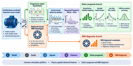
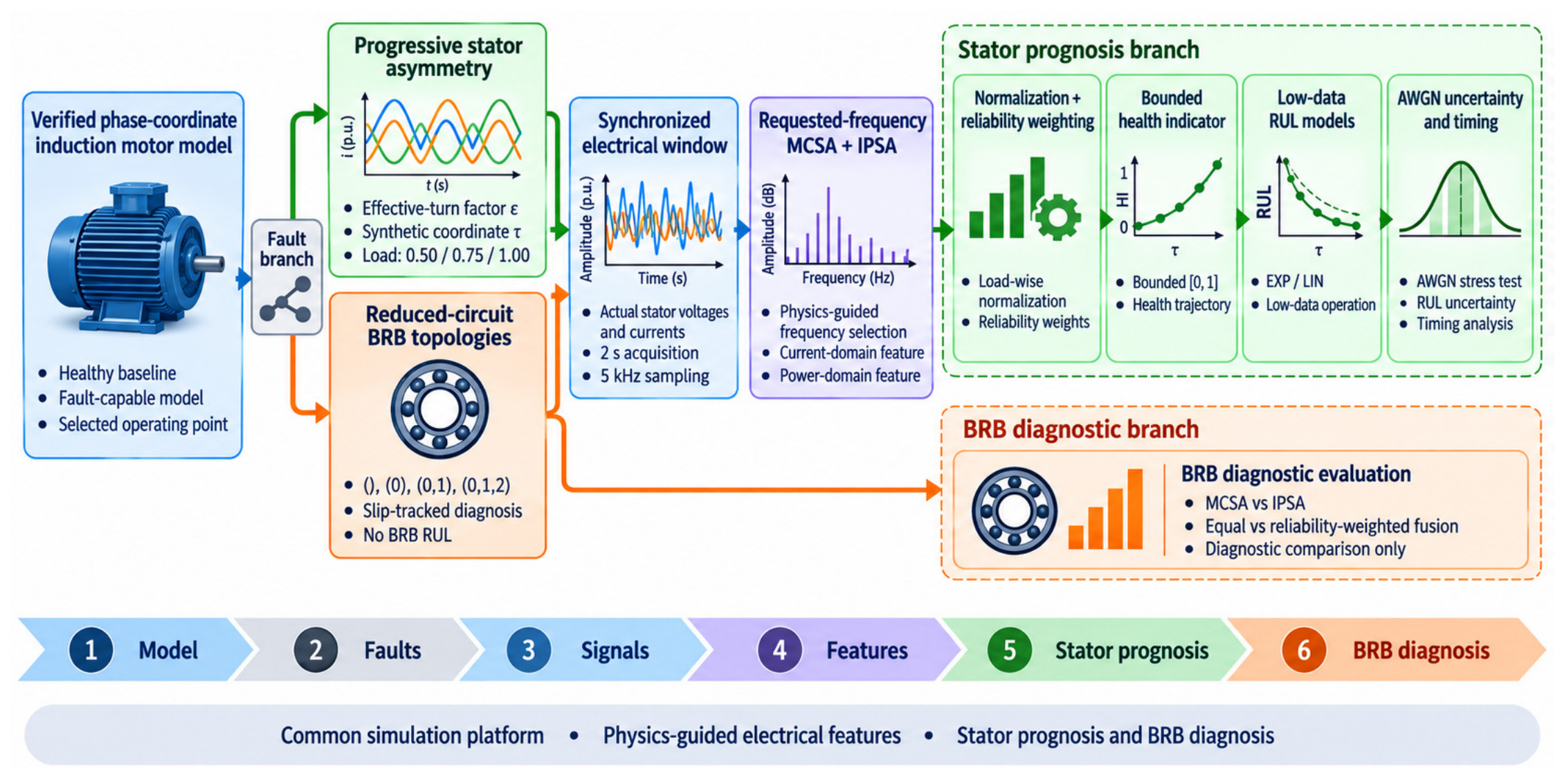
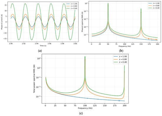
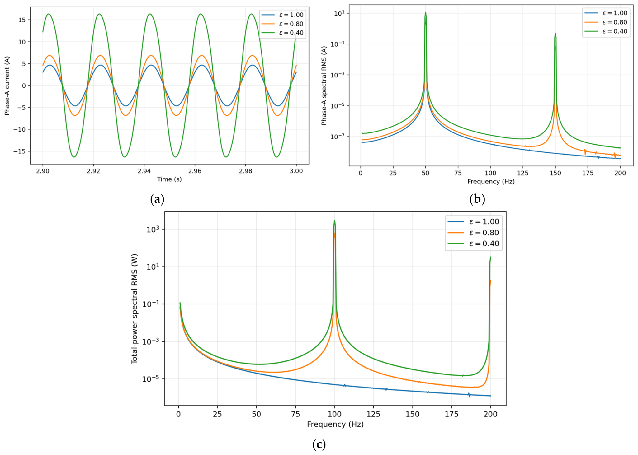
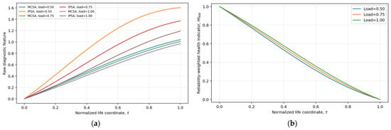
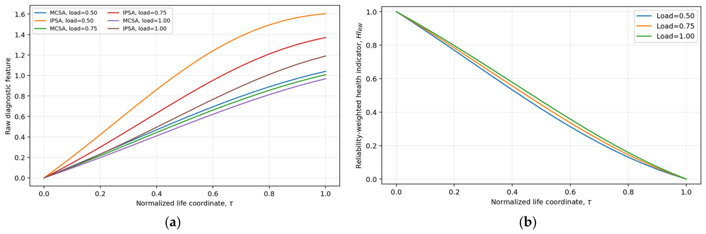
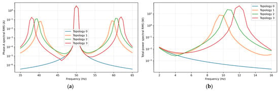
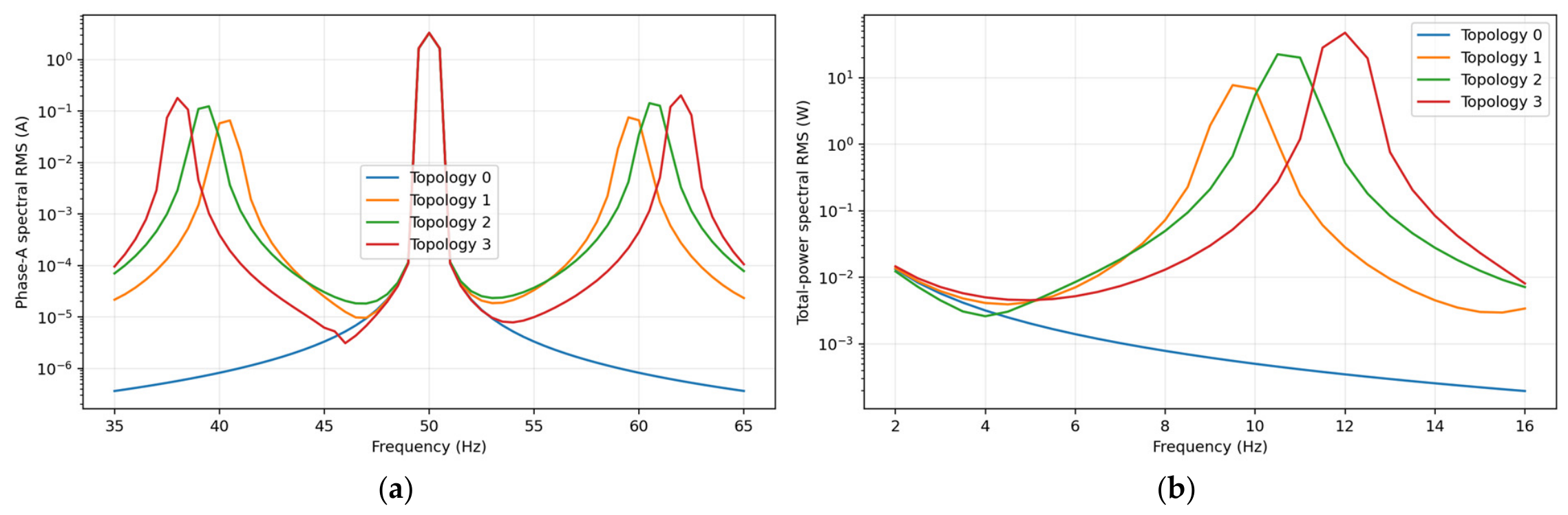
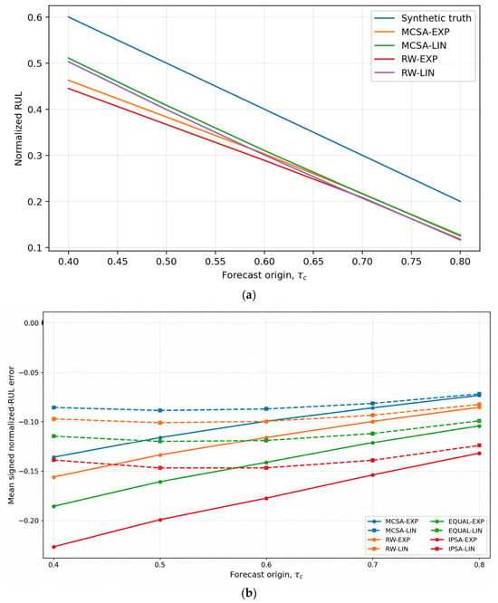
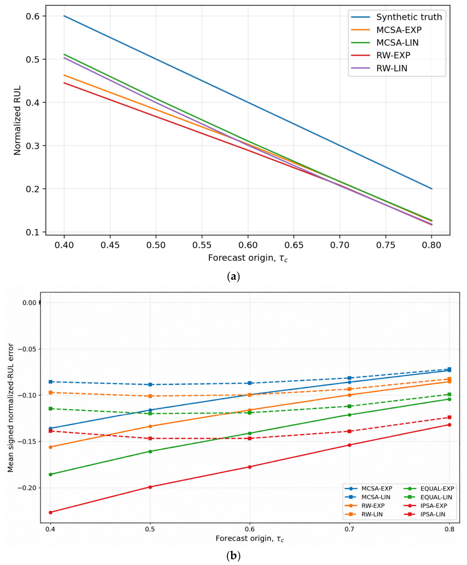
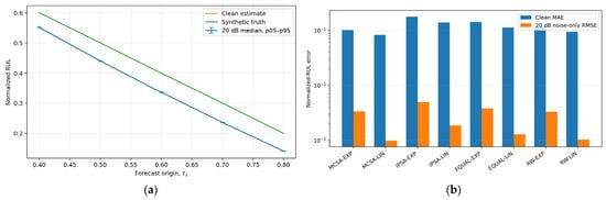
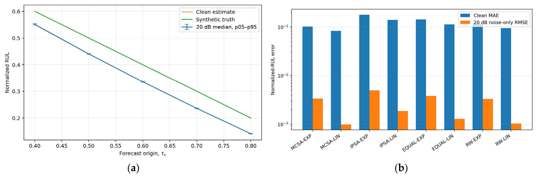
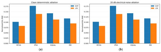
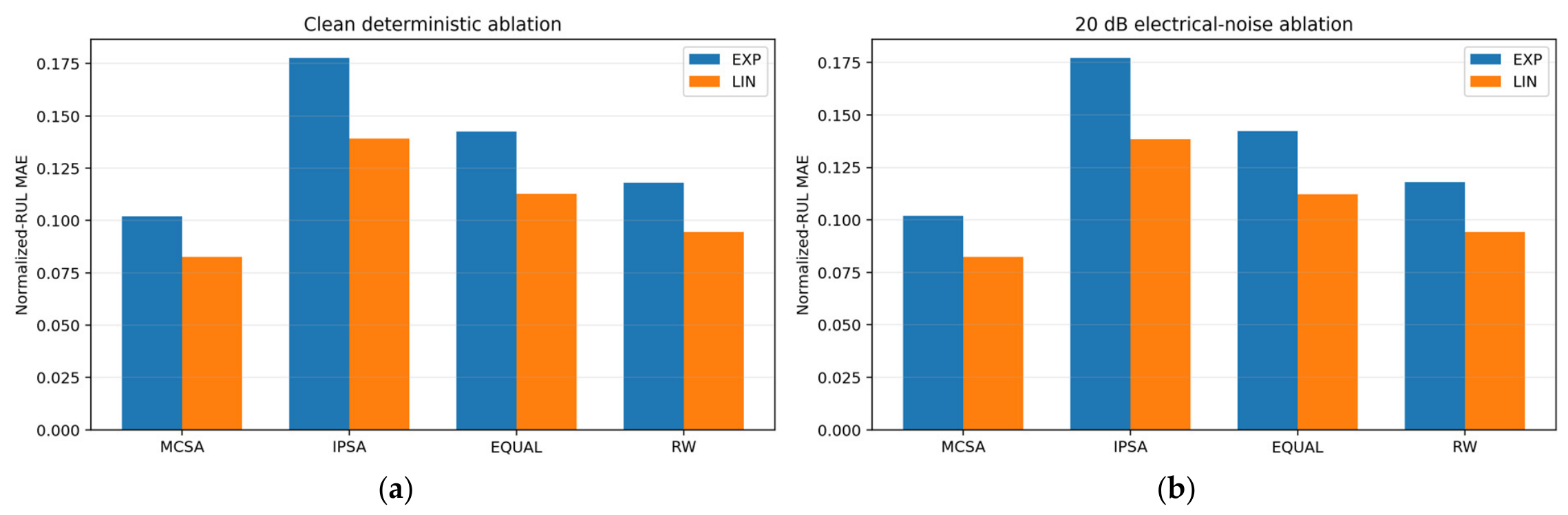
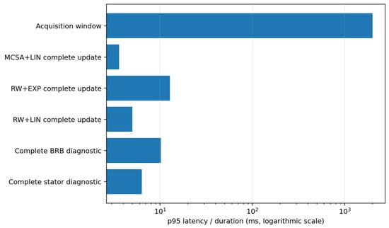
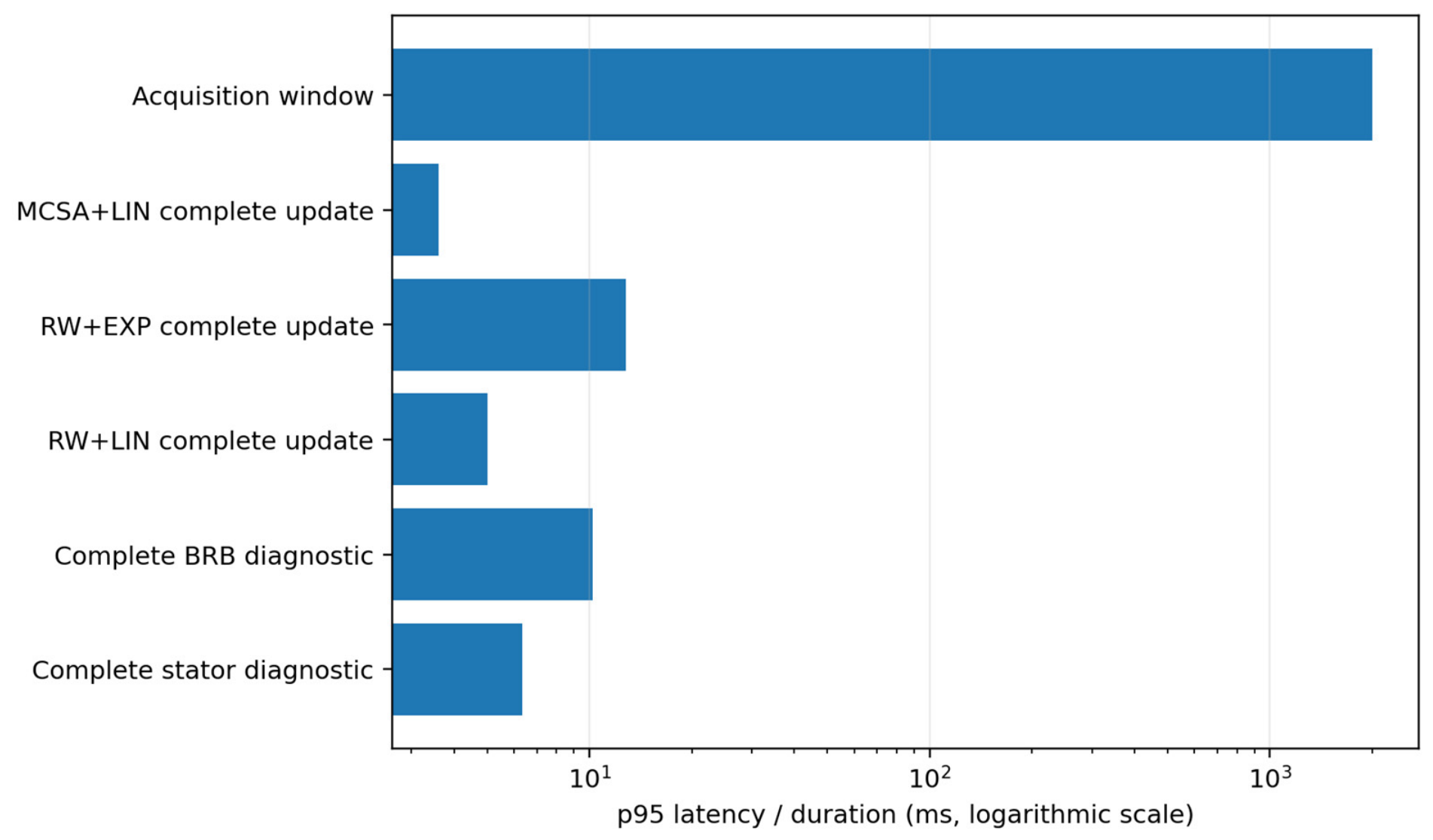

Disclaimer/Publisher’s Note: The statements, opinions and data contained in all publications are solely those of the individual author(s) and contributor(s) and not of MDPI and/or the editor(s). MDPI and/or the editor(s) disclaim responsibility for any injury to people or property resulting from any ideas, methods, instructions or products referred to in the content. |
© 2026 by the author. Licensee MDPI, Basel, Switzerland. This article is an open access article distributed under the terms and conditions of the Creative Commons Attribution (CC BY) license.