


Abstract
High-resolution atmospheric modeling over topographically complex coastal zones requires multi-source spatial data fusion to bridge the scale gap between satellite-assimilated global reanalysis and localized boundary layer dynamics. This study presents a spatial data fusion framework coupling convection-permitting Weather Research and Forecasting (WRF) simulations (3 km grid spacing) with machine learning calibration and GIS multi-criteria decision analysis across continuous computational grids (24,871 cells). Focusing on a high-resolution seasonal case study during the peak Caribbean Low-Level Jet (CLLJ) and Trade Winds regime along the Colombian Caribbean coast, predictive algorithms were benchmarked across day-grouped and Leave-One-Station-Out (LOSO) spatial transfer protocols against classical meteorological baselines. Support Vector Regression (SVR) with an RBF kernel achieved superior residual calibration (, m/s) under day-grouped cross-validation, and an average Leave-One-Station-Out (LOSO) spatial transfer RMSE of m/s under blind geographic transfer to unmonitored stations, corresponding to a >76% RMSE reduction relative to raw, uncalibrated WRF output in that same spatial-transfer setting. Chronological forward-forecasting tests further showed that this seasonally augmented kernel model does not extrapolate reliably to calendar months absent from training (), so a reduced 8-variable configuration is recommended for genuine forward forecasting into unseen seasons. Scalar calibrations were transferred to horizontal wind vectors preserving simulated flow direction, and vertically scaled to 80 m hub height using WRF prognostic shear. Calibrated fields were integrated into a Boolean GIS-MCDA model incorporating wind power density, slope limits, environmental/indigenous reserves, and infrastructure proximity. The framework delineated an high-feasibility macro-corridor (2214 cells; ≈19,926 ) in northern La Guajira, while substantially reducing uncalibrated mesoscale overestimation in the sheltered wake of the Sierra Nevada de Santa Marta. The methodology provides a robust screening-level tool for coastal renewable resource assessment.
1. Introduction
Accurate characterization of near-surface atmospheric dynamics in coastal transition zones is critical for regional climate diagnostics, renewable resource assessment, and environmental planning [1,2]. Coastal territories are governed by intense atmosphere–ocean–land interactions, including sharp surface roughness discontinuities, land–sea thermal contrasts, and localized orographic forcing that generate mesoscale phenomena such as coastal low-level jets, thermal breeze convergence fronts, and localized thermodynamic blocking [3,4]. Resolving these sub-grid interactions represents a fundamental challenge in computational atmospheric sciences and geospatial data fusion [5,6].
Global numerical weather prediction models and atmospheric reanalysis datasets, including ECMWF ERA5 and NOAA Global Forecast System (GFS), assimilate vast volumes of Earth observation and spaceborne remote sensing data, such as MetOp ASCAT scatterometer ocean surface wind vectors, microwave and infrared atmospheric sounders, GNSS radio occultation soundings, and geostationary radiance fields [7,8]. Although these satellite-assimilated datasets capture large-scale synoptic circulations with high fidelity, their typical spatial resolutions (∼25–31 km) and inherent spatial smoothing limit their ability to resolve localized coastal circulations and microclimates over complex topography [9,10]. In coastal zones with steep terrain, global reanalyses frequently underestimate surface drag, smooth out elevated mountain barriers, and misrepresent thermal breeze fronts, leading to systematic regional biases [11,12].
To bridge this spatial representativeness gap, dynamic downscaling using non-hydrostatic mesoscale atmospheric models such as the Weather Research and Forecasting (WRF) model is widely used [13,14]. Configuring WRF at convection-permitting grid spacings (≤3 km) allows explicit numerical resolution of deep convective circulations, thermal breeze systems, and terrain-induced channeling without relying on parameterized cumulus schemes [15,16]. Furthermore, WRF ingestion of high-resolution satellite-derived boundary datasets—such as Shuttle Radar Topography Mission (SRTM) digital elevation models, Moderate Resolution Imaging Spectroradiometer (MODIS) land use classifications, and satellite Optimum Interpolation Sea Surface Temperature (OISST)—substantially improves surface boundary layer representations. Nevertheless, dynamic downscaling alone cannot fully eliminate systematic biases arising from planetary boundary layer (PBL) parameterization uncertainties, unresolved microscale obstacles, and numerical dispersion [17,18]. Consequently, integrating mesoscale simulations with machine learning (ML) post-processing and spatial decision analysis has emerged as an effective paradigm for localized error mitigation [19,20,21].
The Colombian Caribbean offers a compelling environment for coastal atmospheric downscaling. Situated in northern South America, it features the Sierra Nevada de Santa Marta (SNSM), an isolated mountain massif rising from sea level to 5775 m within only 42 km of the coast [16]. The interaction between the macro-scale trade wind inversion, the Caribbean Low-Level Jet (CLLJ), and this massive topographic barrier produces severe horizontal gradients: intense wind acceleration across the semi-arid plains of northern La Guajira and pronounced orographic wind shadows along the sheltered coastlines of Santa Marta, Ciénaga, and Barranquilla [22,23,24]. Standard reanalysis models smooth the SNSM to less than one-third of its actual height, resulting in substantial overestimations of near-surface wind fields in sheltered leeward valleys.
The objective of this research is to formulate, evaluate, and spatially deploy an end-to-end spatial data fusion and machine learning bias correction framework that integrates satellite-assimilated numerical modeling, multi-station in situ observation calibration, and continuous GIS multi-criteria decision analysis (GIS-MCDA) across complex coastal terrain. The study is structured around a high-resolution seasonal case study during the peak-intensity regime of the CLLJ and Trade Winds (February–June), when atmospheric kinetic energy and coastal thermal gradients reach their annual maximum. Importantly, the framework is conceived as a regional screening-level pre-feasibility decision-support tool rather than a definitive micro-siting blueprint, recognizing that bankable wind farm financing requires subsequent multi-year on-site met mast or floating LiDAR campaigns.
This study presents four primary methodological contributions:
- Hierarchical Spatial Data Fusion Pipeline: An integrated workflow linking satellite-assimilated GFS forcing, non-hydrostatic WRF simulations at 3 km grid spacing, in situ surface weather networks, and a direction-preserving vector scaling operator that projects scalar calibrations onto continuous horizontal wind vectors across 24,871 computational cells ().
- Convection-Permitting Mesoscale Modeling: A numerical configuration employing the non-local MYNN 2.5 PBL scheme and high-resolution terrain mapping, explicitly resolving orographic blocking and sea-breeze convergence fronts smoothed by global models [25,26].
- Multi-Model Validation, Spatial Generalization, and Classical Baselines: An empirical benchmarking of candidate predictive algorithms against classical meteorological baselines (Empirical Quantile Mapping and Mean Bias Adjustment) across day-grouped cross-validation (GroupKFold), strict chronological future forecasting, and Leave-One-Station-Out (LOSO) spatial cross-validation to assess blind geographic transferability.
- Screening-Level GIS-MCDA Spatial Feasibility Zoning: A multi-criteria geographic decision framework coupling hub-height thermodynamic wind power density with topographic slope, environmental/indigenous reserves, and logistical infrastructure, reducing overestimation artifacts and delineating realistic high-feasibility macro-corridors.
2. Materials and Methods
2.1. Hierarchical Spatial Data Fusion Architecture
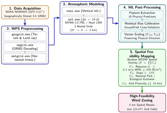
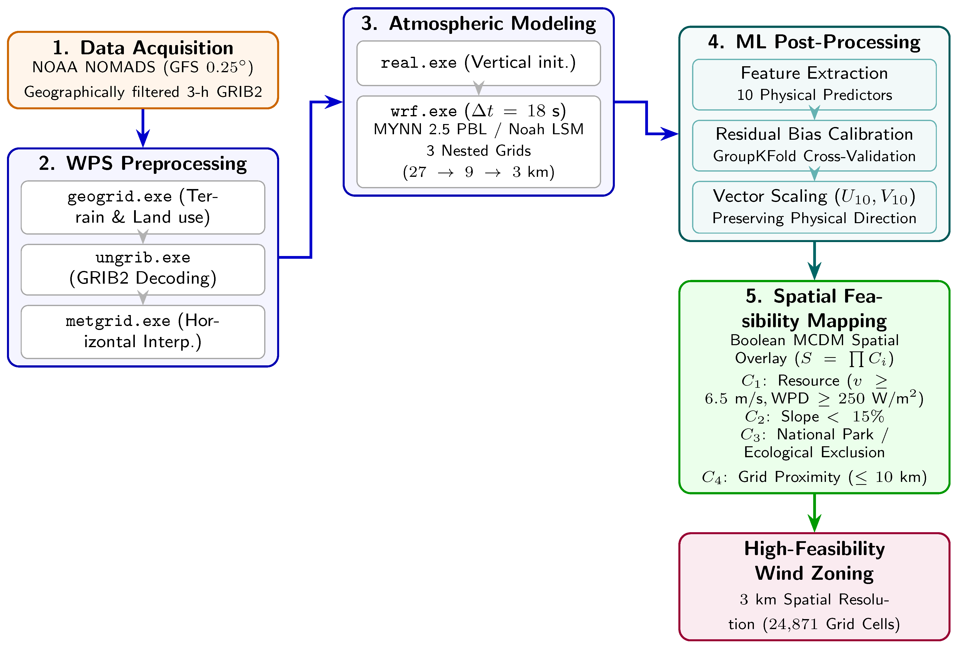
The methodological framework couples satellite-assimilated meteorological data, mesoscale numerical modeling, statistical machine learning post-processing, and geographic information systems into a five-stage spatial data fusion pipeline (Figure 1):
Figure 1.
Hierarchical spatial data fusion pipeline integrating satellite-assimilated synoptic forcing, WRF Preprocessing System (WPS), non-hydrostatic WRF atmospheric solver, machine learning post-processing, and GIS-MCDA spatial feasibility mapping.
- Synoptic Data Ingestion: Global Forecast System (GFS ) atmospheric fields, incorporating spaceborne scatterometer, sounder, and radiance assimilations, are ingested at 3 h intervals.
- Convection-Permitting Atmospheric Downscaling: WRF-ARW is integrated across three nested computational grids down to a native 3 km horizontal spacing ( per grid cell) over the Colombian Caribbean.
- In Situ Ground-Truth Integration and QC: Continuous surface meteorological observations from five automatic weather stations spanning diverse coastal microclimates undergo automated range and flatline quality control.
- Machine Learning Calibration and Vector Scaling: A 10-dimensional physical predictor feature space is compiled from WRF diagnostic outputs to train residual models. A direction-preserving vector scaling operator projects corrected speeds onto the full 2D spatial mesh, followed by vertical extrapolation to hub height.
- GIS-MCDA Spatial Feasibility Zoning:The calibrated continuous fields are coupled with geo-spatial constraint layers (topography, legal/environmental boundaries, grid proximity) using Boolean raster algebra across computational cells.
2.2. Study Area and Topographic Complexity
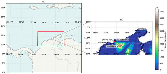
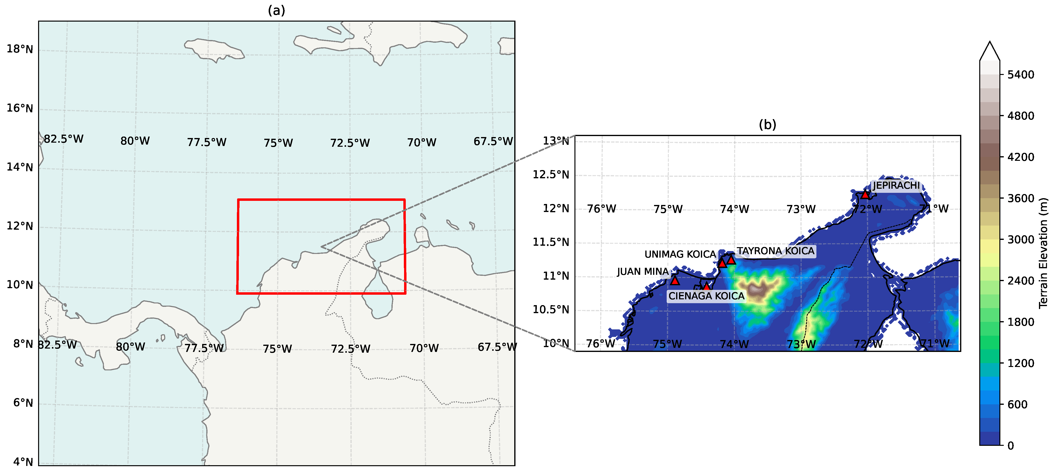
The study area encompasses the Colombian Caribbean coastal territory in northern South America (8° N–14° N, 71° W– 77° W), illustrated in Figure 2. The region displays wide physiographic diversity, transitioning from semi-arid desert coastal plains in Upper La Guajira to dense tropical forests, extensive mangrove wetlands, and the isolated Sierra Nevada de Santa Marta (SNSM) massif, which reaches 5775 m elevation only 42 km from the coastline.
Figure 2.
Geographic location and nesting configuration of the WRF simulation domains (a) and detailed representation of model topography, drainage basins, and meteorological validation stations across the Colombian Caribbean (b).
The regional wind climatology is governed by the macro-scale trade wind inversion and the Caribbean Low-Level Jet (CLLJ), an intense easterly tropospheric wind maximum centered at 925 hPa. When this synoptic jet encounters the SNSM massif, the flow splits into an accelerated maritime stream over northern La Guajira and a severe downwind wake/vortex shedding zone over Santa Marta, Ciénaga, and Barranquilla, creating steep horizontal wind shear gradients over short distances [16,24].
2.3. Seasonal Scope and Temporal Case Study
To evaluate model performance during the annual maximum of atmospheric kinetic energy and land–sea thermal contrast, this study analyzes a high-resolution seasonal evaluation dataset spanning February, March, April, and June 2022 ( validated multi-station daily observation vectors).
This period covers key seasonal phases of the regional climatology:
- Primary Dry Season (February–April): The North Atlantic subtropical high reaches its southernmost position, strengthening the regional pressure gradient and driving peak CLLJ wind speeds (>12 m/s).
- Mid-Summer Transition (June): Strong insolation maximizes land–sea thermal contrasts (), driving vigorous diurnal sea-breeze circulations.
Focusing high-resolution simulations on this high-energy seasonal window ensures that calibration and spatial screening target the period of greatest resource availability and dynamic variability.
2.4. WRF Model Configuration and Numerical Stability
Numerical experiments were executed using the Advanced Research WRF (WRF-ARW) model, version 4.7.1, on a high-performance computing system equipped with 32 physical cores AMD EPYC and 64 GB of RAM.
2.4.1. Domain Configuration and Numerical Integration
Three two-way nested computational domains were configured with horizontal grid spacings of 27 km (outer domain D01), 9 km (intermediate domain D02), and 3 km (innermost domain D03). The innermost domain was discretized into horizontal grid points and 45 vertically stretched terrain-following eta levels, with the lowest level positioned approximately 10 m above the surface.
To ensure numerical stability of the non-hydrostatic governing equations, the model fundamental time step was set to s. This satisfies the operational WRF modeling guideline for grid spacing km [27], ensuring that the non-dimensional Courant number:
remains well within the numerical stability limits of the 3rd-order Runge–Kutta time-integration scheme [28].
2.4.2. Physical Parameterizations
Physical parameterization schemes were selected to represent coastal tropical boundary layer dynamics, summarized in Table 1.
Table 1.
Physical parameterization schemes used in the WRF simulations.
Turbulence and vertical mixing are parameterized using the Mellor–Yamada– Nakanishi–Niino (MYNN) level 2.5 scheme, which resolves a prognostic equation for turbulent kinetic energy (TKE) [29,30,31]. The Noah Land Surface Model (LSM) [32] resolves soil moisture and temperature across four layers to compute sensible () and latent () heat fluxes. In the 3 km innermost domain (D03), cumulus parameterization is disabled, operating in a fully explicit convection-permitting mode [33]. Simulation spin-up artifacts were avoided by discarding the first 6–12 h of each daily forecast cycle [34].
2.4.3. Thermodynamic Wind Power Density Calculation
Wind power density (WPD) was calculated using local air density () computed dynamically at each grid cell from simulated surface pressure () and 2 m air temperature () using the Ideal Gas Law [35]:
where . Across the coastal domain, dynamically varies between and , avoiding the standard constant sea-level approximation () [36]. Wind power density is then computed as:
2.5. Machine Learning Bias Correction and Feature Selection
Machine learning models were trained under the residual learning paradigm [20,37]:
where is the raw simulated wind speed at 10 m.
2.5.1. Hierarchical Feature Selection and Operational Predictor Set
A multi-stage feature selection workflow was formulated to establish an optimal, physically robust predictor space while preventing spatial memorization and elevation-induced overfitting:
- Exploratory Candidate Pool (14 initial candidate variables): An initial pool of 14 variables was assembled, comprising 3 static geospatial/topographic coordinates () and 11 dynamic atmospheric and diurnal variables (, , , , , , , , , , ).
- A Priori Spatial Screening and Physical Feature Selection:
- The 3 static geospatial coordinates () were excluded a priori from the machine learning feature space to eliminate spatial coordinate memorization and artificial elevation-based overfitting, ensuring that the trained estimators learn transferable atmospheric physics rather than localized station coordinates [38,39].
- From the remaining 11 dynamic atmospheric and diurnal variables, 3 variables were pruned: sensible heat flux (, which introduced destabilizing turbulence noise), zonal wind (, weak zonal flow prone to transient microclimatic noise along the dominantly meridional trade wind corridor), and surface pressure (). Although exhibited a strong statistical association with surface wind residuals, it was excluded because it co-varies directly with topographic elevation, functioning as an indirect elevation surrogate that causes artificial overfitting in unmonitored mountainous terrain; its thermodynamic baroclinic effects are safely captured by the sea-air temperature contrast () and planetary boundary layer height ().
- Retaining the remaining 8 dynamic predictors yielded the core 8-variable physical/diurnal baseline set:
- Seasonal Harmonic Augmentation and Final Operational Set (Table 2): To assess model generalization across multi-month synoptic regimes and capture the seasonal progression of the trade-wind cycle (February–June), 2 cyclical harmonic seasonal encodings ( and ) were introduced alongside the 8 core physical features (). This established the 10-variable final operational feature set () summarized in Table 2. The comparative performance of the 8-variable baseline and the 10-variable seasonal configuration is systematically benchmarked in Section 3.Table 2. Optimized set of 10 physical predictor variables used in the machine learning post-processing models.
2.5.2. Direction-Preserving Vector Scaling Algorithm
For each computational grid cell , the trained SVR residual model f predicts the local scalar residual . The calibrated wind speed at 10 m is:
Preserving the original WRF wind direction is physically justified because near-surface wind direction across the Colombian Caribbean is primarily governed by synoptic-scale geostrophic balance, the large-scale sea-level pressure gradient, and macroscopic orographic steering, which are resolved with high kinematic fidelity by WRF’s non-hydrostatic dynamical core. In contrast, the systematic model error is predominantly scalar, originating from surface roughness parameterizations and unresolved boundary layer turbulent momentum dissipation.
To preserve the physical flow trajectories, streamline convergence, and sea-breeze vectors simulated by the atmospheric solver, horizontal vector components are scaled proportionally:
2.6. Vertical Extrapolation to Turbine Hub Height (80 m) and Uncertainty Formulation
Because observational calibration is performed against surface anemometers at 10 m AGL (), calibrated wind fields must be extrapolated to wind turbine hub height ( m) for WPD computation and GIS-MCDA spatial evaluation.
Vertical profile extrapolation is performed using a dynamic power-law formulation:
where is the local dynamic vertical wind shear exponent derived directly from WRF’s prognostic horizontal wind speed profile between the diagnostic 10 m surface level and the model eta level corresponding to approximately 80 m AGL ():
This formulation dynamically preserves the atmospheric stability, thermal stratification, and vertical momentum flux resolved by the MYNN 2.5 PBL scheme at each grid cell, capturing diurnal transitions between convective daytime mixing (– over land) and stable nocturnal/marine surface layers (– over open ocean). In microscale boundary layers, vertical profiles can also be characterized under Monin–Obukhov similarity [40,41]:
where is friction velocity, is the von Kármán constant, is aerodynamic surface roughness dynamically mapped from Noah LSM land cover classes ( m over marine water, – m over coastal scrublands), and is the atmospheric stability correction function dependent on Obukhov length L.
The vertical extrapolation step introduces a critical source of non-linear uncertainty into the resource assessment. Because wind power density scales with the cube of wind speed (), fractional errors in hub-height velocity propagate cubically (). Specifically, a variation in the dynamic shear exponent induces an uncertainty of approximately in and in the resulting WPD. Because tall meteorological masts (≥80 m) and floating offshore LiDAR buoys are currently absent in the Colombian Caribbean, the prognostic WRF-derived shear profile provides the most physically consistent vertical structure available, but must be recognized as a modeled projection that warrants in situ tall-tower validation during subsequent micro-siting phases.
2.7. Data Sources, Weather Stations, and Quality Control
Observational ground-truth datasets were obtained from the Colombian Air Quality Information System (SISAIRE) database and academic networks, including the Unimag-KOICA coastal meteorological observatory. Five automatic weather stations (AWS) equipped with calibrated cup anemometers and wind vanes installed at standard 10 m Above Ground Level (AGL) in strict compliance with World Meteorological Organization guidelines (WMO-No. 8) [42] were selected, detailed in Table 3.
Table 3.
Metadata and geographic characteristics of the meteorological validation stations in the Colombian Caribbean.
To ensure rigorous temporal alignment between continuous hourly AWS observations and discrete WRF model output, station records recorded in local Colombian time (COT, UTC − 5) were converted to Coordinated Universal Time (UTC). Numerical model outputs were archived at hourly intervals coincident with observation timestamps. Spatial matching between observation coordinates and WRF model fields was executed using bilinear spatial interpolation from the four nearest computational grid nodes in innermost domain D03 () to the exact latitude and longitude of each station, extracting the diagnostic 10 m horizontal wind components () directly calculated by the MM5 surface layer scheme to compute .
A standard quality control protocol was applied [42]: physical range filtering ( m/s) and mechanical flatline detection (≥6 consecutive hours of zero variance) [43]. Daily mean wind vectors were computed by aggregating hourly observations and model extractions over 24 h UTC intervals, enforcing a strict completeness filter requiring ≥75% of valid hourly records per day (minimum 18 valid hours) to prevent diurnal sampling bias.
The five monitoring stations capture three distinct physiographic and climatic regimes across the Colombian Caribbean:
- Open Semi-Arid Maritime Corridor: JEPIRACHI (Upper La Guajira) is situated on a low-roughness desert coastal plain ( m) directly exposed to the core of the Caribbean Low-Level Jet (CLLJ) and unobstructed Caribbean Trade Winds.
- Flat Continental Coastal Savannah: JUAN MINA (Atlántico) represents an inland coastal plain with moderate roughness and intermediate exposure.
- Complex Mountain–Coastal Transition Zone: UNIMAG KOICA, TAYRONA KOICA, and CIENAGA KOICA (Magdalena) are situated in the sheltered leeward wake and western foothill slopes of the massive Sierra Nevada de Santa Marta (SNSM), where steep topography (rising from sea level to 5775 m in 42 km) induces intense orographic blocking, localized sea-breeze convergence, and nocturnal catabatic drainage.
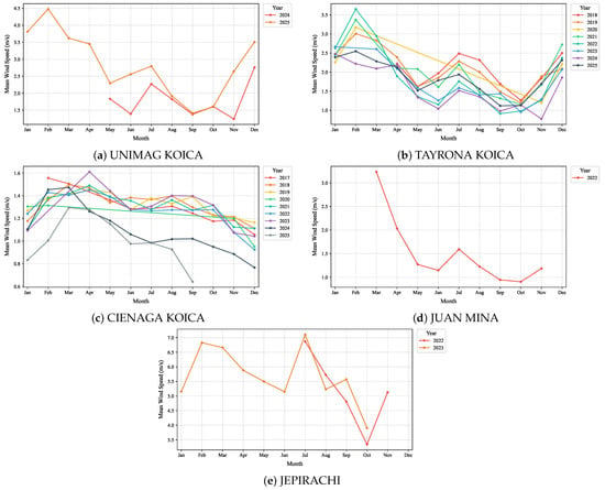
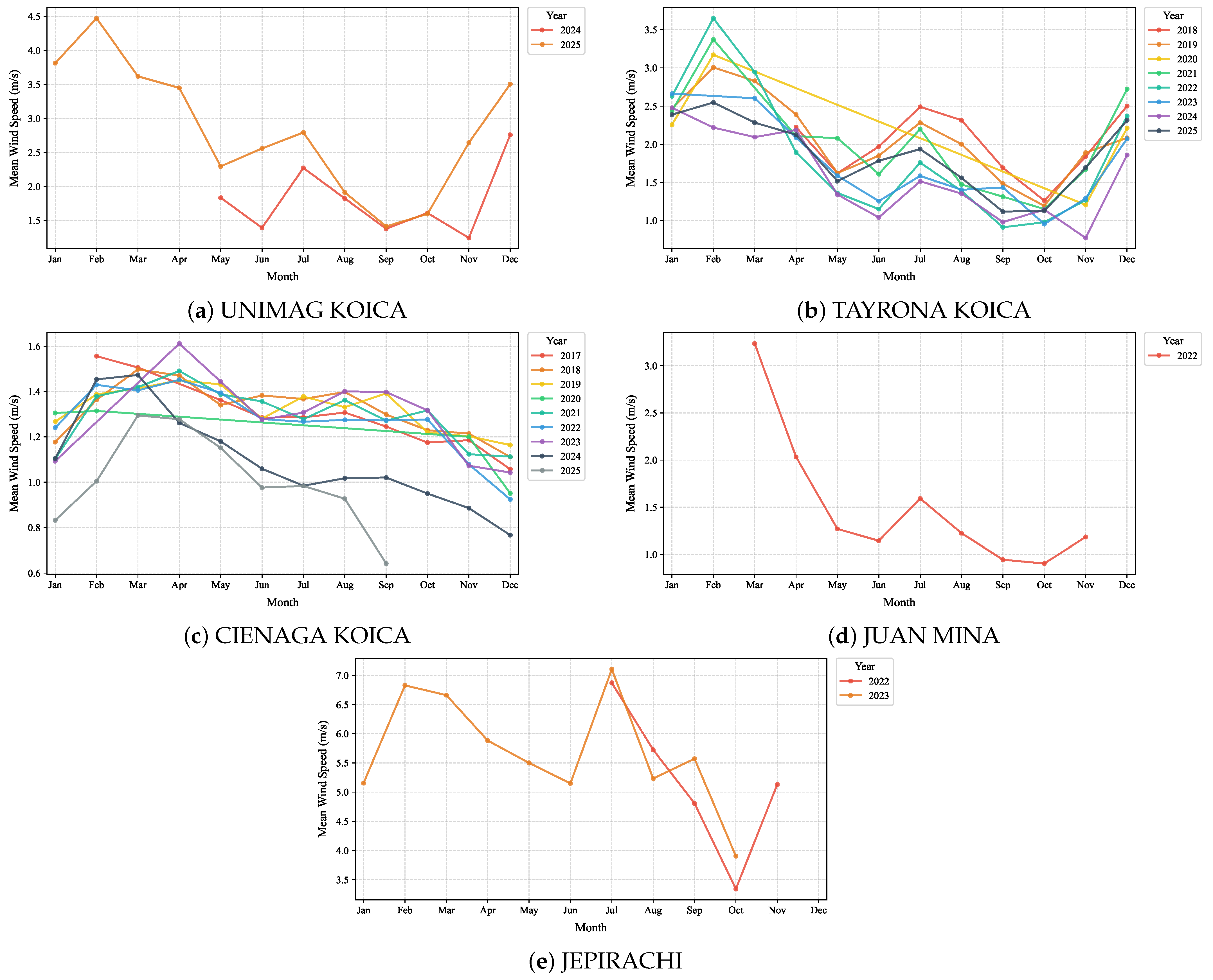
A clear distinction is maintained between two complementary observational datasets: (i) the operational synchronized calibration dataset ( multi-station daily observation vectors across February, March, April, and June 2022), which represents the synchronous multi-station monitoring period strictly coincident with the continuous convection-permitting WRF simulations used for machine learning calibration and spatial mapping; and (ii) multiannual historical observation series, with record lengths that vary by station (ranging from a single year at JUAN MINA to multi-year spans of up to nine years at CIENAGA KOICA and TAYRONA KOICA), which were utilized in Section 3.1 to qualitatively illustrate the seasonal cycle shape at each individual station over the years for which historical data were available. Because these historical windows do not fully overlap across stations, they are not intended as a joint multi-station stability test but as station-specific context for the seasonal cycle.
2.8. Predictive Models and Validation Protocols
A comprehensive suite of predictive models spanning five distinct algorithmic families was implemented:
- Classical Meteorological Baselines:
- –
- Empirical Quantile Mapping (EQM): A non-parametric distribution-matching calibration that maps simulated wind speed quantiles to observed ground truth via empirical cumulative distribution functions: [44].
- –
- Mean Bias Adjustment (MBA / Linear Scaling): Additive climatological correction subtracting the training-set mean error: .
- Multivariate Linear Benchmark: Ordinary Least Squares (OLS) Linear Regression using physical predictor features.
- Tree Ensembles and Gradient Boosting: Random Forest, Extra Trees [45], XGBoost [46], HistGradientBoosting, and LightGBM.
- Kernel Machine Learning: Support Vector Regression (SVR with Gaussian RBF kernel, ).
- Autoregressive Time Series: ARIMA(1,1,1), SARIMA(1,1,1)(1,0,0,7) [14], and Holt–Winters Exponential Smoothing [47].
Feature scaling was performed using ‘StandardScaler’ fitted strictly on training subsets inside each validation split. Five validation schemes were evaluated:
- Day-Grouped Cross-Validation (GroupKFold, 5 Folds): Partitions data strictly by calendar day, ensuring that all 5 station records from any individual synoptic day reside in the same fold. This evaluates model capability to generalize across unseen atmospheric days while preventing intra-day cross-station data leakage [38,39].
- Leave-One-Station-Out Spatial Cross-Validation (LOSO, 5 Folds): To explicitly evaluate spatial generalizability and test whether the learned calibration transfers to completely unmonitored geographic locations across the 24,871 computational cells, a 5-fold spatial cross-validation was conducted where the model is iteratively calibrated on four stations and evaluated strictly on the held-out fifth station.
- Chronological Split (70/15/15): Strict out-of-sample temporal forecast on an unseen future month (June).
- Walk-Forward Rolling Window (5 Folds): Sequential expanding-window evaluation with 20-day horizons.
- Station-Level Evaluation: Disaggregation of predictive metrics across individual stations.
Model performance was assessed using Root Mean Square Error (RMSE), Mean Absolute Error (MAE), Mean Bias, the Coefficient of Determination (), Pearson correlation coefficient (r), and the Root Mean Squared Scaled Error (RMSSE) relative to naive persistence [48]:
where and denote observed and predicted values, represents the arithmetic mean of observed samples in the test evaluation subset, is the residual sum of squares, and is the total sum of squares. Under out-of-sample validation and non-linear machine learning modeling, is bounded in the interval rather than ; negative values indicate that the predictive model yields a higher mean squared error than a naive horizontal benchmark predicting the sample mean () [47].
2.9. GIS Multi-Criteria Decision Analysis (GIS-MCDA) Siting Model
To delineate feasible development corridors across the continuous 24,871-cell spatial mesh (; per cell), a non-compensatory Boolean GIS-MCDA model was formulated [49]:
where a grid cell is classified as feasible () if and only if all four criteria are satisfied simultaneously:
- Wind Resource Availability (): . This threshold corresponds to the NREL Class 3 commercial resource standard [50], representing the lower limit of financial viability for utility-scale turbines (IEC Class II and III). Exclusion occurs if .
- Topographic Slope Constraint (): (). Slopes represent technical and logistical thresholds beyond which crawler crane transit, heavy transport of blades m, and pad construction incur prohibitive civil engineering costs [49].
- Environmental and Legal Exclusions (): inside National Natural Parks (specifically the Sierra Nevada de Santa Marta and Tayrona protected cores), Ramsar wetland sanctuaries (Ciénaga Grande), and constitutionally recognized indigenous reservations, in compliance with Colombian Environmental Law 99/1993, Renewable Energy Law 1715/2014, and Energy Transition Law 2099/2021 [51,52,53].
- Logistical Infrastructure Proximity (): km to coastline, primary national roads, or high-voltage transmission lines (STN kV), establishing an upper bound on balance-of-plant (BOP) interconnection CAPEX.
All input geospatial layers (roads, power lines, reserves, and SRTM digital elevation slope) were reprojected to the geographic reference system WGS84 (EPSG:4326) and harmonized onto the identical WRF D03 computational mesh ( nodes, comprising 24,871 valid onshore/offshore computational cells) using cell-area majority resampling. While multi-criteria decision-making (MCDM) methods utilizing compensatory weighting—such as Analytic Hierarchy Process (AHP), TOPSIS, or Self-Organizing Maps (SOM)—are effective for comparative ranking of multi-attribute energy alternatives [49,54], a non-compensatory Boolean overlay was deliberately chosen for this regional screening phase: legal exclusions (indigenous reserves, national parks) and extreme terrain hazards cannot be compensated for by superior wind speeds [54].
2.10. Time Series Statistical Diagnostics
Stationarity and white-noise properties of post-processed residuals were tested using the Augmented Dickey–Fuller (ADF) test [55], Kwiatkowski–Phillips–Schmidt–Shin (KPSS) test [56], Ljung–Box test (Lag 7) [57], and Durbin–Watson test [58,59].
3. Results
3.1. Time Series Diagnostics and Residual Analysis
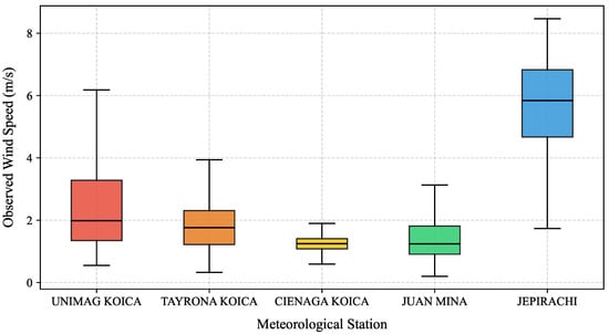
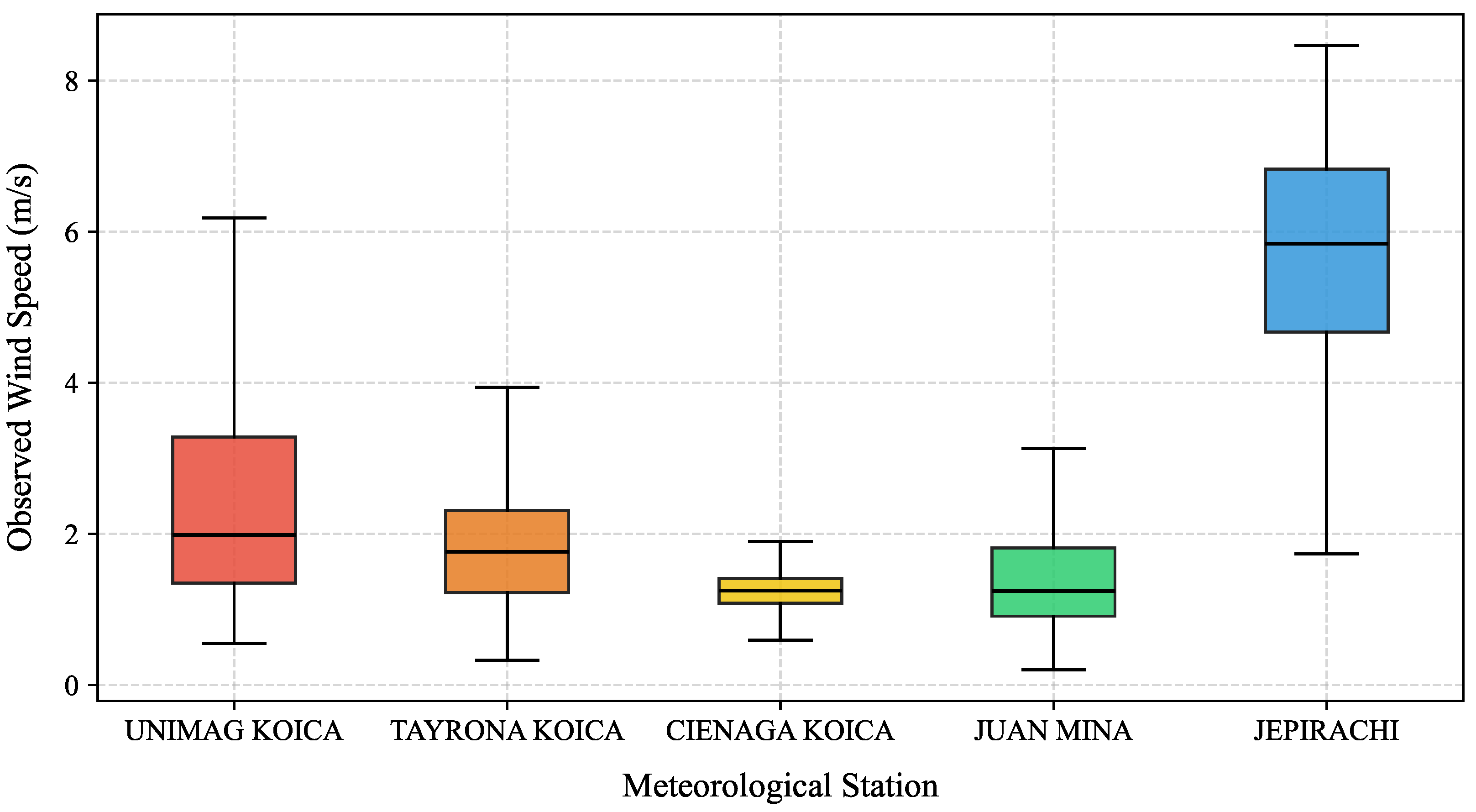
Figure 3 shows observed daily mean wind speed distributions across the five validation stations. JEPIRACHI displays the strongest regime (median observed daily mean of 6.5 m/s and maximum daily mean of 6.83 m/s in the synchronized operational evaluation dataset, with unaggregated instantaneous hourly peaks exceeding 12.0 m/s in raw station anemometer records) beneath the core of the CLLJ. UNIMAG KOICA and TAYRONA KOICA display intermediate regimes (medians 3.2 and 2.8 m/s), whereas CIENAGA KOICA and JUAN MINA reflect sheltered regimes (<1.5 m/s) in the SNSM topographic wake.
Figure 3.
Boxplot distributions of daily mean observed wind speeds across the five regional meteorological stations.
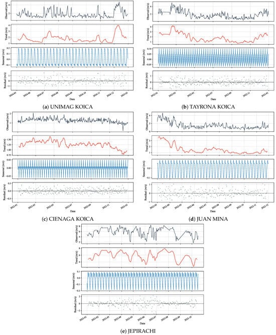
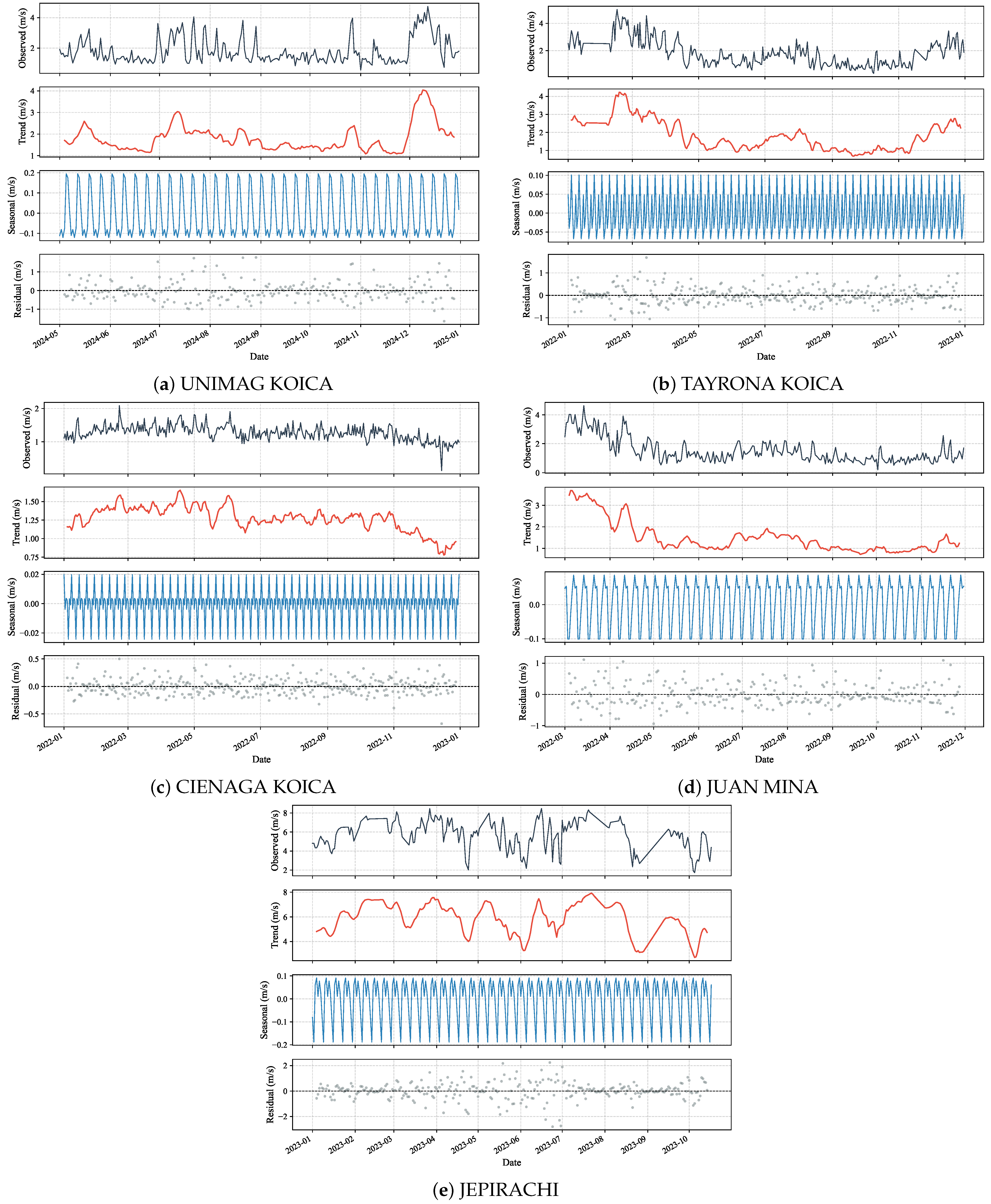
Figure 4 displays the additive seasonal decomposition (7-day period), capturing dry-season downward trends and constant-variance residuals. Figure 5 shows a recurring within-year seasonal shape at each station across the years for which historical records are available; because station record lengths differ and do not fully overlap, this should be read as station-level context rather than a joint cross-station stability test.
Figure 4.
Additive seasonal decomposition (7-day period) of observed daily wind speed across the five coastal stations.
Figure 5.
Historical monthly mean wind speed curves showing multiannual seasonal variability across the five coastal stations.
Stationarity test results (Table 4) indicate that while raw observed wind series fail ADF unit-root tests (), post-processed SVR residuals achieve stationarity at UNIMAG, TAYRONA, CIENAGA, and JEPIRACHI (). At JUAN MINA, SVR residuals remain non-stationary according to ADF (), reflecting persistent localized microclimatic trends. For the complementary KPSS test, the null hypothesis is stationarity, so a series is labeled Non-Stationary whenever and Stationary otherwise; applying this rule consistently, ADF and KPSS agree on non-stationarity for the raw observed wind series at every station, while for SVR residuals the two tests occasionally disagree, which is expected given their different null hypotheses and is not evidence of a computational error.
Table 4.
Results of the Augmented Dickey–Fuller (ADF) and Kwiatkowski–Phillips–Schmidt–Shin (KPSS) stationarity tests applied to observed wind speeds, raw WRF residuals, and SVR-corrected residuals.
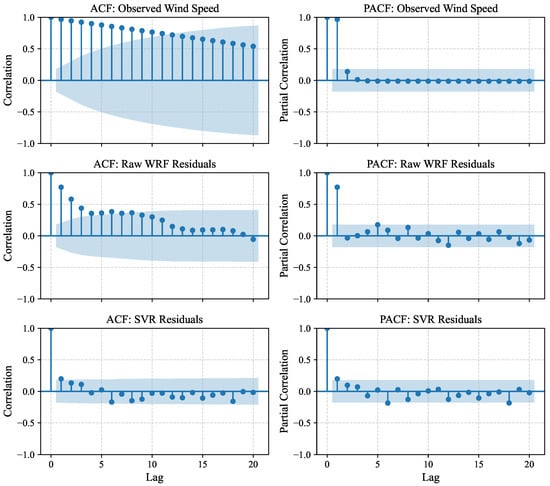
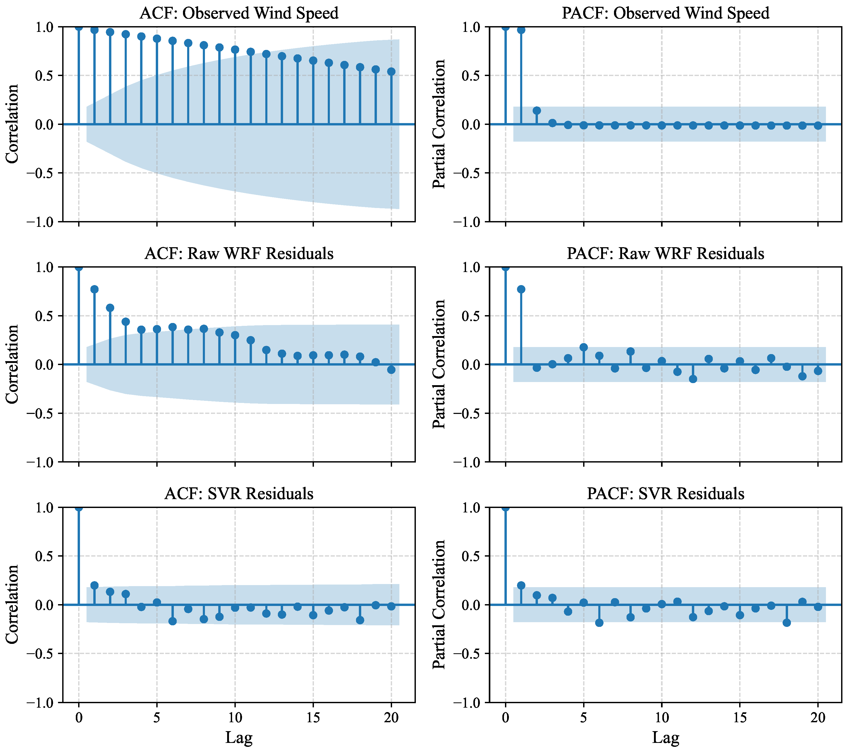
Autocorrelation diagnostics (Table 5 and Figure 6) show that post-processing substantially increases Durbin–Watson statistics (d rises from <0.2 in raw WRF up to –), achieving uncorrelated white-noise residuals at TAYRONA () and CIENAGA (). At UNIMAG, JUAN MINA, and JEPIRACHI, residual autocorrelation remains statistically significant (), indicating unmodeled local turbulence and surface roughness variations.
Table 5.
Results of the Ljung–Box (Lag 7) and Durbin–Watson autocorrelation tests applied to observed wind speeds, raw WRF residuals, and SVR-corrected residuals.
Figure 6.
Autocorrelation Function (ACF) and Partial Autocorrelation Function (PACF) plots up to lag 20 for observed wind speed, raw WRF residuals, and SVR residuals at JEPIRACHI station.
3.2. Multi-Model Performance and Feature Ablation Analysis
Table 6 summarizes cross-validated performance under the primary GroupKFold cross-validation strategy (five folds grouped by calendar day, representing the overall out-of-fold cross-validation average across all five folds). SVR with an RBF kernel outperforms both machine learning algorithms and classical meteorological baselines (, m/s, ), followed closely by Extra Trees () and XGBoost (). Classical meteorologically informed adjustments—Empirical Quantile Mapping (, m/s) and Mean Bias Adjustment (, m/s)—substantially reduce raw WRF error, but are surpassed by SVR by an additional reduction in RMSE. This occurs because univariant quantile or linear scaling corrects the static climatological distribution but is blind to concurrent thermodynamic boundary layer dynamics (), which SVR leverages dynamically. Autoregressive time series models (ARIMA, SARIMA, Exponential Smoothing) fail to capture multi-feature physical forcing ().
Table 6.
Cross-validated performance metrics under the primary GroupKFold validation strategy (overall out-of-fold average across 5 folds grouped by calendar day, with cyclical month encoding).
Table 7 and Table 8 present performance under chronological and walk-forward validation. Across all schemes, SVR consistently maintains the highest predictive accuracy.
Table 7.
Performance metrics under chronological validation (70/15/15 split). Test subset corresponds to an unseen future month (June).
Table 8.
Performance metrics under walk-forward validation (5 sequential folds with a 20-day rolling prediction window).
Table 9 details the generalization gap across four experimental configurations. A key methodological distinction must be emphasized between Table 6 and Table 9: Table 6 presents the overall out-of-fold cross-validation average across all five folds (, m/s) used for comprehensive algorithmic benchmarking, whereas Table 9 evaluates a formal three-way partition (train, validation, and test holdout) specifically designed to quantify the generalization gap, wherein SVR evaluated on the held-out test fold yields and test m/s (gap of ).
Table 9.
Generalization gap analysis and performance metrics (, test RMSE in m/s, test RMSSE, and Train–Test gap) across candidate machine learning models under four feature space and validation configurations.
Under chronological validation with eight variables (Configuration 1), SVR achieves a test with a generalization gap of . When cyclical month features are introduced under chronological partitioning (Configuration 2), SVR experiences an extrapolation collapse in June (, gap ). This occurs because RBF kernels rely on Euclidean distance in Hilbert space; when a future month introduces out-of-distribution coordinates in the plane, kernel weights decay rapidly.
In contrast, GroupKFold (Configurations 3 and 4) samples synoptic days uniformly across the evaluation period while preventing intra-day data leakage across stations. Under GroupKFold with 10 variables (Configuration 4), the generalization gap drops to , achieving test ( m/s).
The comparative evaluation across feature spaces in Table 9 demonstrates the critical role of physical feature selection in constraining model variance and preventing spatial memorization. As detailed in Section 2.5, filtering out destabilizing turbulence noise (), weak zonal noise (), and topography-correlated pressure surrogates () focuses the regression on the primary physical drivers of coastal circulation: surface latent heat exchange (), meridional trade wind momentum (), land–sea thermal contrast (), and boundary layer depth (). Augmenting this core 8-variable physical baseline () with cyclical seasonal harmonics () yields the optimal 10-variable operational feature set (), which attains the highest cross-validated accuracy (, m/s) under GroupKFold validation.
In addition to temporal cross-validation, a Leave-One-Station-Out (LOSO) spatial cross-validation was implemented across the five monitoring sites ( blind spatial folds: iteratively training on four stations and predicting on the held-out fifth station) to rigorously evaluate spatial generalizability and test whether the learned model transfers to unmonitored geographic grid cells. Under blind spatial transfer, SVR achieves: JEPIRACHI (open maritime trade wind plain) m/s (); JUAN MINA (flat continental savannah) m/s (); TAYRONA KOICA m/s (); CIENAGA KOICA m/s (); and UNIMAG KOICA m/s (). The domain-wide mean spatial transfer error is m/s (). Although spatial transfer error to blind stations is naturally higher than day-grouped temporal interpolation ( m/s), it reduces raw WRF mesoscale error ( m/s across stations) by more than . This confirms that the model captures physically transferable boundary layer relationships rather than localized station coordinates.
Table 10 and Table 11 summarize descriptive distributional statistics and station-level disaggregated metrics. Station-level disaggregation in Table 11 quantitatively demonstrates the collapse of WRF’s severe leeward bias behind the Sierra Nevada de Santa Marta (SNSM). At CIENAGA KOICA, raw WRF produces a massive positive bias of m/s (RMSE m/s), which SVR collapses to m/s (RMSE m/s, an error reduction). At UNIMAG KOICA, uncalibrated WRF overestimates wind speed with a bias of m/s (RMSE m/s), which SVR reduces to m/s (RMSE m/s, a reduction). Similarly, at TAYRONA KOICA, raw WRF bias of m/s (RMSE m/s) drops to m/s (RMSE m/s, a reduction). Even in the exposed maritime regime of JEPIRACHI, SVR reduces RMSE from m/s to m/s, bringing domain-mean calibrated wind speed into close alignment with observed ground truth ( m/s vs observed m/s, compared to raw WRF m/s).
Table 10.
Descriptive statistical properties and operational domain metrics of model predictions (wind speed in m/s) across the 4-month evaluation dataset.
Table 11.
Cross-validated station-level performance metrics (RMSE, MAE, RMSSE, and Bias, in m/s) under GroupKFold validation across the five meteorological stations.
3.3. Continuous GIS-MCDA Feasibility Mapping
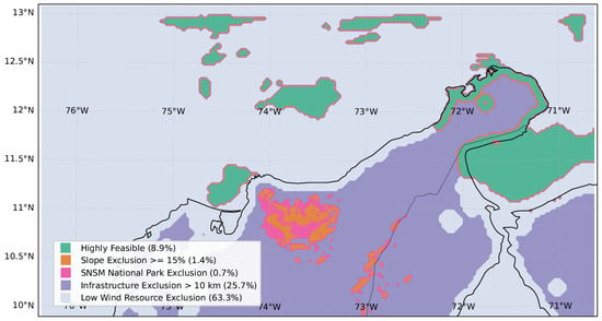
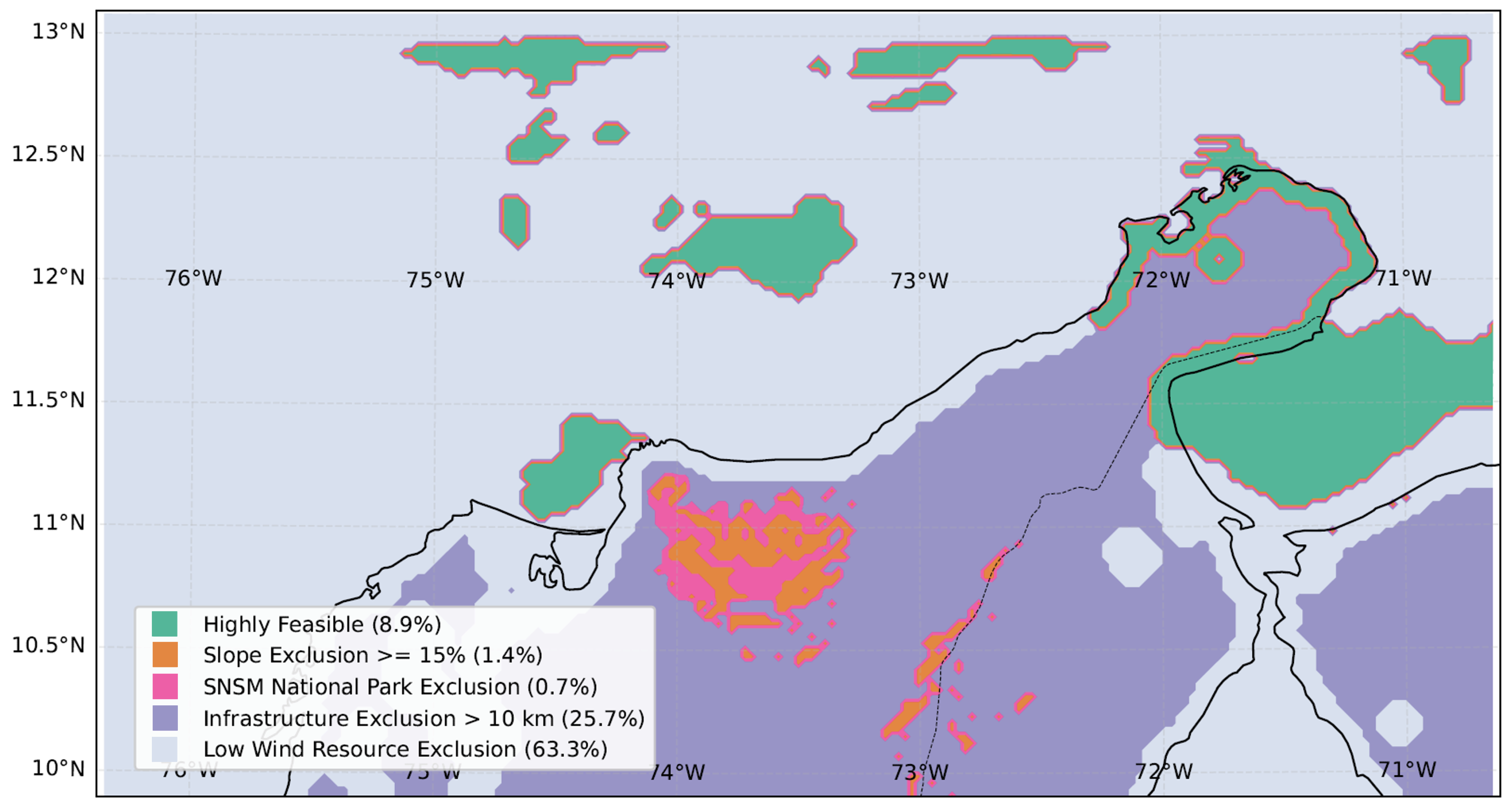
Figure 7 presents the final multi-criteria spatial feasibility zoning across the 24,871 computational grid cells (; per cell). The Boolean spatial overlay classifies of the total study domain (2214 cells; ≈19,926 ) as highly feasible for commercial wind energy development ().
Figure 7.
Multi-criteria spatial feasibility and exclusion mapping for wind energy deployment across the Colombian Caribbean, illustrating suitable development corridors (, ) and specific exclusion layers based on wind resource thresholds (), terrain slope (), legal/environmental reserves in the SNSM (), and grid/infrastructure distance km ().
To establish a transparent, non-ambiguous spatial accounting where individual grid cells may concurrently satisfy multiple exclusion conditions, a hierarchical non-overlapping classification was applied across all computational cells ():
- Feasible Development Macro-Corridor (): 2214 cells ().
- Primary Topographic Exclusion (): 348 cells () with terrain slope .
- Primary Environmental/Legal Exclusion (, non-overlapping with slope): 182 cells () located inside National Natural Parks and indigenous reserves.
- Primary Infrastructure Isolation (, non-overlapping with topography/environment): 6401 cells () located >10 km from grid lines or primary transport links.
- Primary Wind Resource Exclusion (, remaining non-viable domain): cells () failing commercial thresholds ( m/s or W/m2).
The sum of these mutually exclusive categories rigorously equals the entire computational grid: 2214 + 348 + 182 + 6401 + 15,726 = 24,871 cells (). When evaluated independently (allowing spatial overlap), the domain-wide individual exclusion rates are for wind resource deficit (), for infrastructure distance (), for steep slope (), and for environmental and indigenous protection ().
Uncalibrated mesoscale simulations classify of the domain as feasible, with only excluded by wind criteria. Calibrated SVR spatial fusion eliminates overestimation artifacts across the sheltered leeward wake of the Sierra Nevada de Santa Marta while confirming a continuous, high-feasibility macro-corridor in northern La Guajira where sustained CLLJ speeds ( m/s; W/m2) coincide with flat terrain (<15% slope) and accessible infrastructure corridors.
To quantify how variations in decision thresholds affect the feasible spatial envelope, a systematic sensitivity analysis is summarized in Table 12. The macro-corridor varies between (1293 cells) under conservative criteria ( m/s, distance km) and (3009 cells) under relaxed thresholds ( m/s, distance km), confirming that northern La Guajira remains the core robust candidate zone across all plausible planning scenarios.
Table 12.
Systematic sensitivity analysis of the feasible macro-corridor area under perturbations of key GIS-MCDA technical, resource, and infrastructure thresholds.
A spatial uncertainty proxy derived from model residual variance and predictor feature space distance (Area of Applicability, AOA [38]) demonstrates that predictive confidence is highest ( m/s) over the flat coastal plains of La Guajira and nearshore waters, where physical predictor features () remain well within the convex hull of the calibration stations. Uncertainty increases over the rugged transition zones of the SNSM flanks, which are safely eliminated from development consideration by the topographic () and environmental () exclusion filters.
4. Discussion and Methodological Considerations
4.1. Physical Foundations of Machine Learning Residual Calibration
The superior calibration performance of Support Vector Regression (SVR) with an RBF kernel over ensemble decision trees (Random Forest, Extra Trees, XGBoost) and classical meteorological baselines is physically grounded in the continuous, non-linear nature of atmospheric boundary layer dynamics. Numerical mesoscale simulations over steep coastal topographies suffer from two fundamental physical error mechanisms:
- Orographic Drag Under-Representation: At a native 3 km grid spacing, numerical terrain filters smooth the steep 5775 m massif of the Sierra Nevada de Santa Marta (SNSM) into a broader, lower topographic envelope. Consequently, WRF underestimates physical mountain wave drag, sub-grid orographic roughness, and baroclinic flow splitting around the barrier.
- Excessive Vertical Momentum Mixing: The non-local MYNN 2.5 PBL scheme tends to mix horizontal momentum excessively downward from the core of the elevated Caribbean Low-Level Jet (925 hPa) toward the surface layer, artificially flooding sheltered leeward coastal valleys (such as Santa Marta, Ciénaga, and Barranquilla) with high-velocity air, creating systematic positive biases exceeding m/s.
Classical univariate calibration techniques, such as Empirical Quantile Mapping (EQM) or linear mean bias adjustment, adjust the static historical frequency distribution of wind speeds but remain fundamentally blind to concurrent atmospheric thermodynamic stability. In contrast, SVR dynamically integrates boundary layer depth (), land–sea thermal contrast (), and surface latent heat flux (). By mapping these physical covariates into a smooth reproducing kernel Hilbert space (RKHS), SVR applies state-dependent adjustments that vary dynamically between daytime convective mixing and nocturnal stable stratification, explaining why SVR achieves an additional error reduction over Empirical Quantile Mapping.
Furthermore, deliberately excluding static spatial coordinates () and indirect elevation surrogates () prevents artificial spatial memorization, ensuring that the regression learns transferable atmospheric thermodynamics [38].
4.2. Temporal Scope, Validation Trade-Offs, and Spatial Transferability
Evaluating machine learning models across complex terrain requires transparent validation protocols. In this study, the evaluation was structured around a high-resolution seasonal case study focusing on the annual peak kinetic energy window (February–April, June).
The experimental results in Table 9 reveal a critical theoretical trade-off: under strict chronological forward forecasting with seasonal cyclical encodings (Configuration 2), kernel methods suffer an extrapolation collapse on unseen future months (). Mathematically, the Gaussian RBF kernel computes localized similarity:
When predicting an unseen future month (such as June from a February–April training set), the harmonic seasonal features occupy an unvisited geometric quadrant in feature space. Because the Euclidean distance to all support vectors is large, kernel activations decay exponentially toward zero, leaving the decision function dominated solely by the global bias intercept b. Therefore, if the operational goal is forward prediction into genuinely unseen future seasons without historical data, the core 8-variable physical baseline () must be deployed, which preserves stable predictive accuracy (, m/s). Conversely, when developing climatological resource atlases or multi-station spatial calibration over a defined seasonal regime, day-grouped cross-validation (GroupKFold, Configuration 4) is appropriate because it samples all synoptic regimes while preventing intra-day cross-station leakage.
Regarding spatial transferability across the computational cells, the Leave-One-Station-Out (LOSO) spatial cross-validation demonstrates that the model transfers with high accuracy to unmonitored sites across open maritime and coastal savannah regimes (Jepirachi RMSE m/s, Juan Mina RMSE m/s), whereas transfer error increases in complex sheltered foothill terrain (Tayrona, Ciénaga, Unimagdalena RMSE – m/s). Nevertheless, the overall LOSO spatial error of m/s represents a >76.8% reduction relative to uncalibrated WRF mesoscale error ( m/s), validating the physical applicability of the spatial fusion framework. Following Area of Applicability (AOA) concepts [38], the calibrated continuous fields are highly reliable across the coastal shelf, whereas mountainous regions beyond the convex hull of the training data are safely eliminated by topographic and environmental exclusion criteria.
4.3. Vertical Extrapolation and Offshore Remote Sensing Integration
Observational calibration was performed using 10 m AGL surface anemometers, followed by vertical scaling to 80 m hub height using WRF prognostic dynamic shear () and roughness parameters. In coastal boundary layers, strong thermal contrasts between land and sea create steep transitions from daytime convective instability over land to nocturnal stable marine layers over water [40,60].
Because wind power density scales cubically with velocity:
uncertainties in vertical shear propagate non-linearly. A deviation in the dynamic shear exponent induces an uncertainty of in hub-height velocity and in estimated WPD. In the absence of tall meteorological masts (≥80 m) or floating offshore LiDAR buoys in the Colombian Caribbean, the dynamic WRF-derived shear profile provides the most physically consistent vertical structure available, but must be recognized as a modeled projection. Future extensions should incorporate marine remote sensing:
- Floating Doppler LiDAR Systems: Continuous vertical wind vector profiles up to 300 m to calibrate hub-height shear and turbulence intensity directly in offshore development zones [60].
- Spaceborne Synthetic Aperture Radar (SAR): High-resolution Sentinel-1 C-band SAR ocean wind retrievals at spatial resolution and MetOp ASCAT scatterometer observations to provide wide-swath marine ground-truth anchors [61].
4.4. Screening-Level Decision Support and MCDM Framework Comparison
The Boolean GIS-MCDA spatial zoning provides an objective, non-compensatory screening tool for regional energy planning. By eliminating uncalibrated mesoscale overestimations in sheltered coastal valleys downwind of the Sierra Nevada de Santa Marta, the spatial fusion framework prevents misclassifying unviable sites as high-potential corridors.
In sustainable energy planning, decision frameworks are generally categorized into non-compensatory screening models and compensatory multi-criteria decision-making (MCDM) ranking models [49,54]. Recent research, such as the comprehensive study by Dash et al. [54], demonstrates the effectiveness of multi-attribute MCDM models combined with Self-Organizing Maps (SOM) for evaluating and ranking sustainable energy systems under multi-dimensional trade-offs. While compensatory frameworks (such as AHP, TOPSIS, and SOM) allow superior performance in one criterion to offset weaknesses in another, non-compensatory Boolean filtering is essential at the macro-spatial screening phase. Legal constraints (such as indigenous reservations and National Natural Parks under Colombian Laws 99/1993, 1715/2014, and 2099/2021) and extreme slope hazards cannot be compensated for by superior wind resources [54]. Once the feasible macro-corridor is delineated, compensatory MCDM and SOM clustering techniques (as formulated by Dash et al. [54]) can be applied to rank individual parcels and optimize turbine micro-siting based on levelized cost of energy (LCOE), grid interconnection distance, and environmental impact scores.
5. Conclusions
This research developed and evaluated a spatial data fusion and machine learning bias correction framework for convection-permitting atmospheric downscaling and multi-criteria feasibility mapping across complex coastal terrain in the Colombian Caribbean. Coupling 3 km WRF simulations with Support Vector Regression (SVR) and Boolean GIS-MCDA across 24,871 computational cells () resolved mesoscale interactions between the Caribbean Low-Level Jet, coastal thermal circulations, and the steep topography of the Sierra Nevada de Santa Marta.
Key findings include:
- Support Vector Regression (SVR) with an RBF kernel achieved superior post-processing calibration under day-grouped cross-validation (, m/s, interpolating across synoptic days within the calibration period), outperforming tree ensembles, autoregressive benchmarks, and classical meteorological baselines (Empirical Quantile Mapping and Linear Mean Bias Adjustment) by dynamically accounting for atmospheric stability and boundary layer height.
- Leave-One-Station-Out (LOSO) spatial cross-validation confirmed blind geographic transferability, achieving a domain-mean spatial transfer RMSE of m/s across five monitoring stations and reducing raw WRF mesoscale error by >76.8% relative to uncalibrated WRF in that same blind-transfer setting.
- Limitation—seasonal extrapolation: The RBF-kernel SVR is reliable only when interpolating within the distribution of synoptic conditions and calendar months seen during training. Under strict chronological forecasting into a genuinely unseen future month with cyclical seasonal encodings included, the model collapses (, Table 9, Configuration 2), performing worse than a naive mean predictor. Operational forward forecasting into unseen seasons should therefore rely on the reduced 8-variable configuration (Configuration 1, test ) rather than the seasonally augmented model, or be restricted to day-grouped interpolation within an already-observed seasonal window.
- Direction-preserving vector scaling transferred scalar residual corrections onto continuous horizontal wind vectors without distorting physical flow trajectories and convergence lines simulated by the atmospheric core.
- Hierarchical Boolean GIS-MCDA identified an macro-corridor of high feasibility (2214 cells; ≈19,926 ) concentrated in northern La Guajira, while eliminating severe mesoscale overestimation artifacts in the sheltered leeward wake of the Sierra Nevada massif.
Importantly, the present study is structured around a high-resolution seasonal case study during the annual peak-energy Trade Wind/CLLJ regime (February–June), and the resulting feasibility cartography serves as a regional screening-level pre-feasibility decision-support tool. Commercial development and bankable financial commitments require on-site tall meteorological mast (≥80 m) or floating LiDAR campaigns spanning at least 12 continuous months to validate local shear profiles and interannual variability. Future research will focus on assimilating floating LiDAR and coastal radar observations into WRF initial states and extending simulations across multi-decadal reanalyses to evaluate climate change and ENSO teleconnections.
Author Contributions
Conceptualization, A.V.-G., A.O.-C. and C.R.-A.; methodology, A.V.-G. and A.O.-C.; software, A.V.-G. and M.C.-R.; validation, A.V.-G., M.C.-R. and D.R.-L.; formal analysis, A.V.-G., A.O.-C. and D.R.-L.; investigation, A.V.-G., M.C.-R. and A.O.-C.; resources, A.O.-C. and C.R.-A.; data curation, A.V.-G. and M.C.-R.; writing—original draft preparation, A.V.-G., M.C.-R. and A.O.-C.; writing—review and editing, D.R.-L. and C.R.-A.; visualization, A.V.-G. and M.C.-R.; supervision, A.O.-C. and C.R.-A.; project administration, A.O.-C.; funding acquisition, A.O.-C. and C.R.-A. All authors have read and agreed to the published version of the manuscript.
Funding
This research was funded by the Ministerio de Ciencia, Tecnología e Innovación—Fondo Francisco José de Caldas and the Agencia Nacional de Hidrocarburos (ANH), through the Contrato de Financiamiento de Recuperación Contingente No. 112721-053-2025, within the project “Herramientas tecnológicas y prototipos para caracterizar, identificar y optimizar el potencial eólico en zonas costeras de Colombia” (Project Code 111983).
Institutional Review Board Statement
Not applicable.
Informed Consent Statement
Not applicable.
Data Availability Statement
Data Availability Statement: Publicly available atmospheric model analyses and meteorological station datasets were analyzed in this study. NOAA GFS atmospheric data are openly available through the NOAA NOMADS portal (https://nomads.ncep.noaa.gov/) (accessed on 30 August 2026). Surface meteorological observations from SISAIRE can be accessed via the IDEAM portal (http://sisaire.ideam.gov.co/) (accessed on 30 August 2026). Additionally, the simulation outputs, dynamic visualizations, and machine learning post-processing assets generated in this research are openly available in GitLab at (https://gitlab.com/Ukari_plz/simulations_wrf-ml) (accessed on 30 August 2026).
Acknowledgments
The authors acknowledge the high-performance computing resources and meteorological data provided by the Universidad de la Costa (CUC), Universidad del Magdalena and the Universidad Cooperativa de Colombia (UCC).
Conflicts of Interest
The authors declare no conflicts of interest. The funders had no role in the design of the study; in the collection, analyses, or interpretation of data; in the writing of the manuscript; or in the decision to publish the results.
Abbreviations
The following abbreviations are used in this manuscript:
| ADF | Augmented Dickey–Fuller |
| AGL | Above Ground Level |
| ASCAT | Advanced Scatterometer |
| AWS | Automatic Weather Station |
| CFL | Courant–Friedrichs–Lewy |
| CLLJ | Caribbean Low-Level Jet |
| DEM | Digital Elevation Model |
| ENSO | El Niño-Southern Oscillation |
| ERA5 | ECMWF Reanalysis 5th Generation |
| GFS | Global Forecast System |
| GIS | Geographic Information System |
| HistGBT | Histogram-based Gradient Boosting |
| KPSS | Kwiatkowski–Phillips–Schmidt–Shin |
| LiDAR | Light Detection and Ranging |
| LSM | Land Surface Model |
| MAE | Mean Absolute Error |
| MCDA | Multi-Criteria Decision Analysis |
| ML | Machine Learning |
| MODIS | Moderate Resolution Imaging Spectroradiometer |
| MYNN | Mellor–Yamada–Nakanishi–Niino |
| NREL | National Renewable Energy Laboratory |
| OISST | Optimum Interpolation Sea Surface Temperature |
| PBL | Planetary Boundary Layer |
| QC | Quality Control |
| RBF | Radial Basis Function |
| RMSE | Root Mean Square Error |
| RMSSE | Root Mean Squared Scaled Error |
| RRTMG | Rapid Radiative Transfer Model for GCMs |
| SAR | Synthetic Aperture Radar |
| SISAIRE | Sistema de Información sobre Calidad del Aire |
| SNSM | Sierra Nevada de Santa Marta |
| SRTM | Shuttle Radar Topography Mission |
| SVR | Support Vector Regression |
| TKE | Turbulent Kinetic Energy |
| WPD | Wind Power Density |
| WPS | WRF Preprocessing System |
| WRF | Weather Research and Forecasting |
References
- Pryor, S.C.; Barthelmie, R.J.; Bukovský, M.S.; Leung, L.R.; Makhniaeva, K. Climate change impacts on wind power generation. Nat. Rev. Earth Environ. 2020, 1, 627–643. [Google Scholar] [CrossRef] [Scilit]
- Elshafei, B. Offshore Wind Resource Assessment Based on Scarce Spatio-Temporal Measurements Using Matrix Factorization. SSRN Electron. J. 2022; Preprint. [CrossRef] [Scilit]
- Ahmad, S.; Abdullah, M.; Kanwal, A.; Tahir, Z.u.R.; Saeed, U.B.; Manzoor, F.; Atif, M.; Abbas, S. Offshore wind resource assessment using reanalysis data. Wind Eng. 2022, 46, 1173–1186. [Google Scholar] [CrossRef] [Scilit]
- Ryu, G.H.; Kim, Y.G.; Kwak, S.J.; Choi, M.S.; Jeong, M.S.; Moon, C.J. Atmospheric Stability Effects on Offshore and Coastal Wind Resource Characteristics in South Korea for Developing Offshore Wind Farms. Energies 2022, 15, 1305. [Google Scholar] [CrossRef] [Scilit]
- Salvação, N.; Guedes Soares, C. Wind resource assessment offshore the Atlantic Iberian coast with the WRF model. Energy 2018, 145, 276–287. [Google Scholar] [CrossRef] [Scilit]
- Hahmann, A.N.; Rostkier-Edelstein, D.; Warner, T.T.; Givati, A. Wind climate estimation using WRF model output: Method and model sensitivities over the sea. Int. J. Climatol. 2015, 35, 3422–3439. [Google Scholar] [CrossRef] [Scilit]
- Hersbach, H.; Bell, B.; Berrisford, P.; Hirahara, S.; Horányi, A.; Muñoz-Sabater, J.; Nicolas, J.; Peubey, C.; Radu, R.; Schepers, D.; et al. The ERA5 global reanalysis. Q. J. R. Meteorol. Soc. 2020, 146, 1999–2049. [Google Scholar] [CrossRef] [Scilit]
- Hallgren, C.; Aird, J.A.; Ivanell, S.; Körnich, H.; Vakkari, V.; Barthelmie, R.J.; Pryor, S.C.; Sahlée, E. Machine learning methods to improve spatial predictions of coastal wind speed profiles and low-level jets using single-level ERA5 data. Wind Energy Sci. 2024, 9, 821–840. [Google Scholar] [CrossRef] [Scilit]
- Hahmann, A.N.; Sīle, T.; Witha, B.; Davis, N.N.; Dörenkämper, M.; Ezber, Y.; García-Bustamante, E.; González-Rouco, J.F.; Navarro, J.; Olsen, B.T.; et al. The making of the New European Wind Atlas—Part 1: Model sensitivity. Geosci. Model Dev. 2020, 13, 5053–5078. [Google Scholar] [CrossRef] [Scilit]
- Wasson, G.; Panda, S.K. Sensitivity of PBL parameterization schemes in simulating lightning and thunderstorm using WRF-ELEC model. Clim. Dyn. 2024, 62, 3799–3821. [Google Scholar] [CrossRef] [Scilit]
- Cañadillas, B.; Wang, S.; Ahlert, Y.; Djath, B.; Barekzai, M.; Foreman, R.; Lampert, A. Coastal horizontal wind speed gradients in the North Sea based on observations and ERA5 reanalysis data. Meteorol. Z. 2023, 32, 207–228. [Google Scholar] [CrossRef] [Scilit]
- Baas, A.C. Systematic under-representation of ERA5 10 m wind speeds in the ERA5-land product undermines wind energy studies. Appl. Energy 2026, 412, 127634. [Google Scholar] [CrossRef] [Scilit]
- Al Oqaily, A.; Giani, P.; Crippa, P. Evaluating WRF Multiscale Wind Simulations in Complex Terrain: Insights from the Perdígao Field Campaign. J. Geophys. Res. Atmos. 2025, 130, e2025JD044055. [Google Scholar] [CrossRef] [Scilit]
- Bin Nadeem, T.; Naqvi, A.A.; Saad, M.; Malik, K.; Ahmed, A. Offshore wind resource assessment and 7E analysis of offshore wind farms on the coastal belt of Pakistan. Process Saf. Environ. Prot. 2025, 202, 107673. [Google Scholar] [CrossRef] [Scilit]
- Prein, A.F.; Langhans, W.; Fosser, G.; Ferrone, A.; Ban, N.; Goergen, K.; Keller, M.; Tölle, M.; Gutjahr, O.; Feser, F.; et al. A review on regional convection-permitting climate modeling: Demonstrations, prospects, and challenges. Rev. Geophys. 2015, 53, 323–361. [Google Scholar] [CrossRef] [Scilit] [PubMed]
- Gil Ruiz, S.A.; Cañón Barriga, J.E.; Martínez, J.A. Assessment and validation of wind power potential at convection-permitting resolution for the Caribbean region of Colombia. Energy 2022, 244, 123127. [Google Scholar] [CrossRef] [Scilit]
- Gómez-Navarro, J.J.; Raible, C.C.; Dierer, S. Sensitivity of the WRF model to PBL parametrisations and nesting techniques: Evaluation of wind storms over complex terrain. Geosci. Model Dev. 2015, 8, 3349–3363. [Google Scholar] [CrossRef] [Scilit]
- Shiferaw, A.; Tadesse, T.; Rowe, C.; Oglesby, R. Weather Research and Forecasting Model (WRF) Sensitivity to Choice of Parameterization Options over Ethiopia. Atmosphere 2024, 15, 974. [Google Scholar] [CrossRef] [Scilit]
- García-Santiago, O.; Hahmann, A.N.; Badger, J.; Peña, A. Evaluation of wind farm parameterizations in the WRF model under different atmospheric stability conditions with high-resolution wake simulations. Wind Energy Sci. 2024, 9, 963–979. [Google Scholar] [CrossRef] [Scilit]
- Zhang, W.; Tian, M.; Hai, S.; Wang, F.; An, X.; Li, W.; Li, X.; Sheng, L. Improving the Forecasts of Coastal Wind Speeds in Tianjin, China Based on the WRF model with Machine Learning Algorithms. J. Meteorol. Res. 2024, 38, 570–585. [Google Scholar] [CrossRef] [Scilit]
- Salcedo-Sanz, S.; Ortiz-García, E.G.; Pérez-Bellido, A.M.; Portilla-Figueras, A.; Prieto, L. Short term wind speed prediction based on evolutionary support vector regression algorithms. Expert Syst. Appl. 2011, 38, 4052–4057. [Google Scholar] [CrossRef] [Scilit]
- Pinilla, A.; Rodríguez, C.; Trujillo, J. Performance evaluation of Jepirachi Wind Park. Renew. Energy 2009, 34, 48–52. [Google Scholar] [CrossRef] [Scilit]
- Robles-Algarín, C.; Restrepo-Leal, D.; Ospino-Castro, A. Feasibility Analysis of Offshore Wind Power Projects in the Caribbean Region of Colombia: A Case Study Using FAHP–GIS. Sustainability 2023, 15, 16620. [Google Scholar] [CrossRef] [Scilit]
- Guillot, J.; Restrepo Leal, D.; Robles-Algarín, C.; Oliveros, I.; Niño-Suárez, P.A. Wind power prediction using a nonlinear autoregressive exogenous model network: The case of Santa Marta, Colombia. Int. J. Electr. Comput. Eng. 2023, 13, 4856–4867. [Google Scholar] [CrossRef] [Scilit]
- Dudhia, J. Numerical study of convection observed during the winter monsoon experiment using a mesoscale two-dimensional model. J. Atmos. Sci. 1989, 46, 3077–3107. [Google Scholar] [CrossRef] [Scilit]
- Kong, X.; Wang, A.; Bi, X.; Sun, B.; Wei, J. The Hourly Precipitation Frequencies in the Tropical-Belt Version of WRF: Sensitivity to Cumulus Parameterization and Radiation Schemes. J. Clim. 2022, 35, 285–304. [Google Scholar] [CrossRef] [Scilit]
- Skamarock, W.C.; Klemp, J.B.; Dudhia, J.; Gill, D.O.; Barker, D.M.; Duda, M.G.; Huang, X.Y.; Wang, W.; Powers, J.G. A Description of the Advanced Research WRF Version 3; NCAR Tech. Note NCAR/TN-475+STR; National Center for Atmospheric Research: Boulder, CO, USA, 2008; 113p. [Google Scholar] [CrossRef] [Scilit]
- Courant, R.; Friedrichs, K.; Lewy, H. Über die partiellen Differenzengleichungen der mathematischen Physik. Math. Ann. 1928, 100, 32–74. [Google Scholar] [CrossRef] [Scilit]
- Nakanishi, M.; Niino, H. An improved Mellor–Yamada level-3 model: Its numerical stability and application to a regional model. Bound.-Layer Meteorol. 2006, 119, 397–407. [Google Scholar] [CrossRef] [Scilit]
- Nakanishi, M.; Niino, H. Development of an improved turbulence closure model for the atmospheric boundary layer. J. Meteorol. Soc. Jpn. Ser. II 2009, 87, 895–912. [Google Scholar] [CrossRef] [Scilit]
- Keshtgar, M.; Siadatmousavi, S.M. Sensitivity analysis of WRF model to physical parameterization for the characterization of coastal and offshore wind patterns in Caspian Sea region. Theor. Appl. Climatol. 2024, 156, 10. [Google Scholar] [CrossRef] [Scilit]
- Gholami, S.; Ghader, S.; Khaleghi-Zavareh, H.; Ghafarian, P. Sensitivity of WRF-simulated 10 m wind over the Persian Gulf to different boundary conditions and PBL parameterization schemes. Atmos. Res. 2021, 247, 105147. [Google Scholar] [CrossRef] [Scilit]
- Lu, Y.; Marsham, J.H.; Tang, J.; Parker, D.J.; Fang, J. Summer Mesoscale Convective Systems in Convection-Permitting Simulation Using WRF Over East China. J. Geophys. Res. Atmos. 2025, 130, e2025JD043653. [Google Scholar] [CrossRef] [Scilit]
- Thundathil, R.; Zus, F.; Dick, G.; Wickert, J. Assimilation of GNSS tropospheric gradients into the Weather Research and Forecasting (WRF) model version 4.4.1. Geosci. Model Dev. 2024, 17, 3599–3616. [Google Scholar] [CrossRef] [Scilit]
- Lehneis, R. Effects of Climate Change on Wind Power Generation: A Case Study for the German Bight. Energies 2025, 18, 3287. [Google Scholar] [CrossRef] [Scilit]
- ISO 2533:1975; Standard Atmosphere. ISO: Geneva, Switzerland, 1975. Available online: https://www.iso.org/standard/7472.html (accessed on 31 August 2026).
- Sun, Y.; Qian, Y.; Jiang, X.; Wang, T.; Wang, L.; Zhu, C. Predicational biases investigation between the WRF and the COAWST models for offshore wind resource. IET Conf. Proc. 2025, 2025, 529–533. [Google Scholar] [CrossRef] [Scilit]
- Meyer, H.; Reudenbach, C.; Hengl, T.; Katurji, M.; Nauss, T. Improving performance of spatio-temporal machine learning models using forward feature selection and target-oriented validation. Environ. Model. Softw. 2018, 101, 1–9. [Google Scholar] [CrossRef] [Scilit]
- Roberts, D.R.; Bahn, V.; Ciuti, S.; Boyce, M.S.; Elith, J.; Guillera-Arroita, G.; Hurlbert, A.; Leathwick, J.R.; Lehmann, A.; Paul, J.; et al. Cross-validation strategies for data with temporal, spatial, hierarchical or phylogenetic structure. Ecography 2017, 40, 913–929. [Google Scholar] [CrossRef] [Scilit]
- Monin, A.S.; Obukhov, A.M. Basic laws of turbulent mixing in the surface layer of the atmosphere. Tr. Akad. Nauk SSSR Geofiz. Inst. 1954, 24, 163–187. [Google Scholar]
- Arya, S.P. Introduction to Micrometeorology; Academic Press: San Diego, CA, USA, 2001; Volume 79, Available online: https://www.sciencedirect.com/book/9780120593545/introduction-to-micrometeorology (accessed on 31 August 2026).
- World Meteorological Organization. Guide to Instruments and Methods of Observation (WMO-No. 8), 2018 edition, updated 2021 ed.; WMO: Geneva, Switzerland, 2018; Available online: https://library.wmo.int/records/item/41650-guide-to-instruments-and-methods-of-observation (accessed on 31 August 2026).
- Zhao, L.; Wang, C.; Jiang, Y.; Xu, J. Research on the characteristics of wind speed, wind direction, and wind profile based on ERA5 reanalysis data. Aerosp. Traffic Saf. 2024, 1, 131–140. [Google Scholar] [CrossRef] [Scilit]
- Themeßl, M.J.; Gobiet, A.; Leuprecht, A. Empirical-statistical downscaling and error correction of daily precipitation from regional climate models. Int. J. Climatol. 2011, 31, 1530–1544. [Google Scholar] [CrossRef] [Scilit]
- Saranya, S.; Rajasenathipathi, M. Machine Learning Based Weather Forecasting for Enhanced Solar Energy Optimization. Int. J. Sci. Res. (IJSR) 2026, 15, 435–439. [Google Scholar] [CrossRef] [Scilit]
- Ma, X.; Liu, Y.; Jie, Y.; Han, S. Assessment Method of Offshore Wind Resource Based on Multi-dimensional Indexes System. CSEE J. Power Energy Syst. 2024, 10, 77–88. [Google Scholar] [CrossRef] [Scilit]
- Hyndman, R.J.; Athanasopoulos, G. Forecasting: Principles and Practice, 3rd ed.; OTexts: Melbourne, Australia, 2021; Available online: https://otexts.com/fpp3/ (accessed on 31 August 2026).
- Makridakis, S.; Spiliotis, E.; Assimakopoulos, V. The M5 accuracy competition: Results, findings, and conclusions. Int. J. Forecast. 2022, 38, 1346–1364. [Google Scholar] [CrossRef] [Scilit]
- Al-Yahyai, S.; Charabi, Y.; Gastli, A.; Al-Badi, A.H. Wind farm land suitability indexing using multi-criteria analysis. Renew. Energy 2012, 44, 80–87. [Google Scholar] [CrossRef] [Scilit]
- Elliott, D.L.; Holladay, C.G.; Barchet, W.R.; Foote, H.P.; Sandusky, W.F. Wind Energy Resource Atlas of the United States; Technical Report DOE/CH/10093-4; Pacific Northwest Lab.: Richland, WA, USA; Solar Energy Research Inst.: Golden, CO, USA, 1986. [Google Scholar]
- Congreso de la República de Colombia. Ley 99 de 1993: Por la Cual se Crea el Ministerio del Medio Ambiente, se Reordena el Sector Público Encargado de la Gestión y Conservación del Medio Ambiente y los Recursos Naturales Renovables; Diario Oficial No. 41.146; Función Pública: Bogotá, Colombia, 1993. Available online: http://www.secretariasenado.gov.co/senado/basedoc/ley_0099_1993.html (accessed on 31 August 2026).
- Congreso de la República de Colombia. Ley 1715 de 2014: Por Medio de la Cual se Regula la Integración de las Energías Renovables no Convencionales al Sistema Energético Nacional; Diario Oficial No. 49.151; Función Pública: Bogotá, Colombia, 2014. Available online: http://www.secretariasenado.gov.co/senado/basedoc/ley_1715_2014.html (accessed on 31 August 2026).
- Congreso de la República de Colombia. Ley 2099 de 2021: Por Medio de la Cual se Dictan Disposiciones para la Transición Energética, la Dinamización del Mercado Energético y la Reactivación Económica del País; Diario Oficial No. 51.731; Función Pública: Bogotá, Colombia, 2021. Available online: http://www.secretariasenado.gov.co/senado/basedoc/ley_2099_2021.html (accessed on 31 August 2026).
- Dash, S.; Chakravarty, S.; Giri, N.C.; Ghugar, U.; Fotis, G. Performance Assessment of Different Sustainable Energy Systems Using Multiple-Criteria Decision-Making Model and Self-Organizing Maps. Technologies 2024, 12, 42. [Google Scholar] [CrossRef] [Scilit]
- Dickey, D.A.; Fuller, W.A. Distribution of the estimators for autoregressive time series with a unit root. J. Am. Stat. Assoc. 1979, 74, 427–431. [Google Scholar] [CrossRef] [Scilit]
- Kwiatkowski, D.; Phillips, P.C.; Schmidt, P.; Shin, Y. Testing the null hypothesis of stationarity against the alternative of a unit root: How sure are we that economic time series have a unit root? J. Econom. 1992, 54, 159–178. [Google Scholar] [CrossRef] [Scilit]
- Ljung, G.M.; Box, G.E. On a measure of lack of fit in time series models. Biometrika 1978, 65, 297–303. [Google Scholar] [CrossRef]
- Durbin, J.; Watson, G.S. Testing for Serial Correlation in Least Squares Regression: I. Biometrika 1950, 37, 409–428. [Google Scholar] [CrossRef] [Scilit]
- Durbin, J.; Watson, G.S. Testing for Serial Correlation in Least Squares Regression: II. Biometrika 1951, 38, 159–178. [Google Scholar] [CrossRef] [Scilit]
- Peña, A.; Gryning, S.E.; Hasager, C.B.; Floors, R.; Courtney, M. Ten Years of Boundary-Layer and Wind-Power Meteorology at Høvsøre, Denmark. Bound.-Layer Meteorol. 2016, 158, 1–26. [Google Scholar] [CrossRef] [Scilit]
- Hasager, C.B.; Vincent, C.; Badger, M.; Badger, J.; Di Bella, A.; Peña, A.; Husson, R.; Mouche, A. Using Satellite SAR to Characterize the Wind Flow around Offshore Wind Farms. Energies 2015, 8, 5413–5439. [Google Scholar] [CrossRef] [Scilit]

Disclaimer/Publisher’s Note: The statements, opinions and data contained in all publications are solely those of the individual author(s) and contributor(s) and not of MDPI and/or the editor(s). MDPI and/or the editor(s) disclaim responsibility for any injury to people or property resulting from any ideas, methods, instructions or products referred to in the content. |
© 2026 by the authors. Licensee MDPI, Basel, Switzerland. This article is an open access article distributed under the terms and conditions of the Creative Commons Attribution (CC BY) license.